
Submitted:
10 November 2025
Posted:
11 November 2025
You are already at the latest version
Abstract
Small and Medium-sized Enterprises (SMEs) face disproportionately high risks from Advanced Persistent Threats (APTs), which often evade traditional cybersecurity measures. Existing frameworks catalogue adversary tactics and defensive solutions but provide limited quantitative guidance for allocating limited resources under uncertainty, a challenge amplified by the growing use of AI in both offensive operations and digital forensics. This paper proposes a game-theoretic model for improving Digital Forensic Readiness (DFR) in SMEs. The approach integrates the MITRE ATT&CK and D3FEND frameworks to map APT behaviours to defensive countermeasures and defines 32 custom DFR metrics, weighted using the Analytic Hierarchy Process (AHP), to derive utility functions for both attackers and defenders. The main analysis considers a non-zero-sum attacker–defender bimatrix game and yields a single Nash equilibrium in which the attacker concentrates on Impact-oriented tactics and the defender on Detect-focused controls. In a synthetic calibration across ten organisational profiles, the framework achieves a median readiness improvement of 18.0% (95% confidence interval: 16.3% to 19.7%) relative to pre framework baselines, with targeted improvements in logging and forensic preservation typically reducing key attacker utility components by around 15–30%. A zero-sum variant of the game is also analysed as a robustness check and exhibits consistent tactical themes, but all policy conclusions are drawn from the empirical non-zero-sum model. Despite relying on expert-driven AHP weights and synthetic profiles, the framework offers SMEs actionable, equilibrium-informed guidance for strengthening forensic preparedness against advanced cyber threats.
Keywords:
Digital Forensic Readiness
; Advanced Persistent Threats (APT)
; resource constraints
; small and medium-sized enterprises (SMEs)
; MITRE ATT&CK
; MITRE D3FEND
; Game Theory
; cybersecurity
; security threats
; Artificial Intelligence (AI)
; cybersecurity awareness
1. Introduction
Digital forensic readiness (DFR) enables organizations to proactively collect and preserve admissible digital evidence, reducing legal risks and supporting business continuity. It is particularly valuable for Small and Medium-sized Businesses and Enterprises (SMBs/SMEs)—encompassing both the commercial/business context (SMB) and the broader organizational/industrial context (SME)—which often face resource constraints in cybersecurity operations. A robust DFR strategy ensures that significant cyber incidents can be addressed efficiently, lawfully, and professionally, conserving investigative resources, reducing costs, protecting organizational reputation, and maintaining compliance with applicable regulations.
Despite heavy investment in Computer Security Incident Response Teams (CSIRTs), Digital Forensics and Incident Response (DFIR) units, and advanced monitoring technologies—such as EDR, XDR, NDR, SIEM, and IDPS—organizations still struggle to achieve effective incident detection and response. Such limitations become especially pronounced against Advanced Persistent Threats (APTs), which are sophisticated, well-funded actors conducting prolonged cyber campaigns APTs are stealthy, long term cyberattacks by unauthorized entities to remain undetected in networks [1,2,3]. Recent threat intelligence reports indicate that while global median dwell time has decreased to 11 days, this metric rises significantly when organizations rely on external notifications (median 26 days), highlighting the importance of internal detection capabilities [4]. Data breaches impose severe financial consequences on organizations; the global average cost reached USD 4.44 million in 2025, with financial sector breaches averaging USD 6.08 million [4,5]. Historical data suggest that cyber incidents can have devastating impacts on small enterprises, with earlier studies indicating that a substantial portion may face severe operational disruptions following major breaches [6]. For example, Baker [7] notes that in the SolarWinds incident, threats persisted within networks for prolonged periods without detection.
The rapid proliferation of artificial intelligence (AI) has further complicated this landscape. AI-driven tools empower attackers with advanced automation, adaptive tactics, and the ability to launch more sophisticated and targeted attacks, thereby increasing the potency of APTs. Conversely, while AI offers defenders enhanced capabilities for faster and more accurate detection, it also introduces unprecedented forensic challenges. These include the complexity of analyzing AI-generated attacks, the potential for AI-based evidence manipulation, and the need for new techniques to handle AI-related incidents. For SMBs, these challenges are particularly acute due to resource constraints. These technical challenges are compounded by the broader organizational struggle to effectively govern AI systems and mitigate associated risks, a problem highlighted in recent literature [8].
Organizations often perceive this issue as primarily technical in nature. However, this challenge fundamentally encompasses the interplay of technology, human expertise, and processes. Without skilled personnel and planning, even the most advanced technology stack may fail against determined assailants. Situations where inadequate DFR hinders effective cyber security incident investigations—often due to poor data retention, ineffective log management, or compromised digital evidence integrity—exemplify what we term non-forensicability (see Section 5.1 for a detailed discussion). Wrightson [9] emphasizes that understanding an attacker’s motivations and capabilities, as well as knowing their past actions, helps investigators categorize and respond to diverse cyber threats.
Digital forensic investigators must know both defense and offense strategies, preempt emerging attack techniques, and collaborate closely with defense teams. Årnes [10] characterizes digital forensics, as a sub-discipline of forensic science, as encompassing scientifically validated methods for the management of digital evidence. These methods are essential for reconstructing criminal incidents or anticipating unauthorized activities.
To address the need for a formal strategic framework for DFR, we propose a game-theoretic approach to model the strategic interactions between cyber attackers and defenders. This approach helps organizations anticipate threats, optimize defense strategies, and make more informed decisions. We focus on the strategic behavior in digital forensics, drawing from Sun Tzu’s wisdom in `The Art of War,’ which emphasizes the importance of understanding both one’s own abilities and the opponent’s strengths and strategies. As Tzu [11] states, “If you know the enemy and know yourself, you need not fear the result of a hundred battles. If you know yourself but not the enemy, for every victory gained, you will also suffer a defeat. You will succumb in every battle if you know neither the enemy nor yourself.” This highlights the importance of knowing the adversary’s motivations, methods, and goals, as well as the capabilities and limitations of one’s own tools and techniques.
Inspired by Sun Tzu’s philosophy, our game-theoretic model operationalizes this wisdom by quantifying how knowledge asymmetries between attacker and defender impact forensic readiness. We operationalize “know yourself” via 16 defender metrics (Table 8) that quantify organizational capabilities, and “know the enemy” via 16 attacker utilities (Table 7) that model adversary behaviors. These 32 metrics are linked through an explicit ATT&CK↔D3FEND coupling that yields measurable forensic readiness improvements and richer post-incident evidence. We formalize three strategic states: comprehensive knowledge (targeted defense), partial knowledge (vulnerable defense), and ignorance (minimal resilience). This approach is especially important in the AI era, where modeling emerging AI-powered attack surfaces and their forensic implications becomes essential for building resilient systems.
Game theory provides a mathematical foundation for analyzing strategic interactions among rational decision-makers [12]. Its application in cybersecurity is growing, as it offers a structured approach to:
- Model Strategic Decisions: Capture the objectives and constraints of both attackers and defenders [13].
- Conduct Risk Analysis: Elucidate payoffs and tactics to identify critical vulnerabilities and optimal defensive strategies [14].
- Enable Adaptive Defense: Capture the dynamic nature of cyber threats, including those augmented by AI, to inform adaptive countermeasures [15].
- Optimize Resource Allocation: Evaluate strategy effectiveness to guide efficient investment of limited defensive resources [16].
To operationalize this game-theoretic approach, our methodology is grounded in established cybersecurity standards and formal decision-making processes. We build upon best practices from the National Institute of Standards and Technology (NIST) for metric development and forensic readiness [17]. Specifically, we integrate the MITRE ATT&CK framework to systematically model adversary behaviors and the complementary MITRE D3FEND framework to map defensive countermeasures. This integration provides a standardized taxonomy that bridges attacker tactics with defender responses. Based on these frameworks, we define 32 custom DFR metrics, weighted using the Analytic Hierarchy Process (AHP), to compute quantifiable utility functions for both attackers and defenders. This addresses a critical gap in the field: the absence of quantifiable payoffs in strategic DFR planning. Furthermore, we present an end-to-end algorithmic suite for scoring, classification, and gap analysis, moving beyond fragmented assessments towards a holistic readiness model.
This paper makes the following key contributions:
- A novel game-theoretic model for DFR that quantifies strategic attacker-defender interactions.
- The integration of MITRE ATT&CK and D3FEND with AHP-weighted metrics to ground utilities in real-world tactics and techniques.
- An equilibrium analysis that yields actionable resource allocation guidance for SMBs/SMEs.
- An evaluation demonstrating the framework’s efficacy in reducing attacker success rates, even in complex, multi-vector APT scenarios influenced by modern AI-powered tools.
The remainder of this paper is structured as follows: Section 2 reviews the related works in digital forensics investigation and readiness. Section 3 describes our game-theoretic approach and algorithms for DFR. Section 4 presents our experimental analysis and results. Section 5 concludes with our findings and future work.
2. Related Works
Enhancing cybersecurity and digital forensics has spurred a plethora of studies. These foundational works span technical defenses, strategic modeling, and simulation of cyber interactions. While appreciating their contributions, we identify areas for further exploration.
2.1. Game Theory in Digital Forensics
Alpcan et al. [18] provided a foundational contribution to the field of network security by presenting theoretical approaches for decision-making in security from a game-theoretic perspective. Their work serves as a valuable reference not only for researchers and graduate students but also for practitioners such as system administrators and security officers seeking to apply quantitative models grounded in control, optimization, and decision theory. Casey [19] established the conceptual foundation for incorporating game theory into digital forensics, contextualizing how strategic analysis can enhance forensic practices.
Manshaei et al. [20] offered a comprehensive overview of game-theoretic methods in network security and privacy, highlighting their capability to model strategic interactions in complex adversarial environments. Their study provided in-depth insights into how game theory can strengthen computer and communication network security across multiple layers, including physical and MAC layers, self-organizing networks, intrusion detection systems, anonymity and privacy mechanisms, network security economics, and cryptography. The authors summarized key concepts such as equilibrium analysis and mechanism design, emphasizing the significance of addressing information limitations and learning factors in developing effective security solutions.
Several subsequent studies have built on this foundation to explore game-theoretic applications in digital forensics. Nisioti et al. [21] presented a Bayesian game model for analyzing interactions between a forensic investigator and a strategic attacker on a multi-host forensic investigation graph. Hasanabadi et al. [22] developed a model representing attacker–investigator dynamics involving rootkits and anti-rootkits, defining each player’s actions and profiling their characteristics. Extending these ideas, Karabiyik et al. [23] proposed a game-theoretic approach to optimize tool selection in digital forensics, particularly focusing on file carving tools and the strategic adaptation of selection decisions during investigations. Hasanabadi et al. [24] later introduced a memory-based mechanism to expand action spaces within forensic game models, reducing convergence iterations when new anti-forensic or counter-anti-forensic tools emerge. Caporusso et al. [25] further analyzed post-attack decision dynamics in human-controlled ransomware scenarios, modeling negotiation strategies and emphasizing the role of information availability, user education, and human factors in developing resilient defensive responses.
2.2. Digital Forensics Readiness and Techniques
Kebande et al. [26] introduced a technique for implementing DFR in cloud computing environments through a modified obfuscated Non-Malicious Botnet (NMB). Operating as a distributed forensic Agent-Based Solution (ABS), this method enables forensic logging for readiness purposes across cloud infrastructures. In a related effort, Kebande et al. [27] proposed the construction of a Digital Forensic Readiness Intelligence Repository (DFRIR) founded on knowledge-sharing principles. The repository cross-references potential evidence sources, aims to reduce the time required for forensic investigations, and supports sharing across multiple jurisdictions.
Englbrecht et al. [28] developed a DFR-specific Capability Maturity Model (CMM) to guide organizations in implementing readiness measures. The framework draws on COBIT 5 IT-Governance principles and incorporates the core characteristics necessary for effective DFR implementation. Reddy et al. [29] built a Digital Forensic Readiness Management System (DFRMS) tailored for large organizations. Based on requirements identified through a comprehensive literature review, the DFRMS architecture comprises five modules: event analysis, DFR information management, costing, access control, and user interface. A proof-of-concept prototype demonstrated the system’s practical feasibility and its potential to improve readiness in enterprise contexts.
Grobler et al. [30] positioned DFR as a means to strengthen organizational security strategies by preparing for incidents while minimizing disruptions to business processes. Their guidelines emphasize ensuring legal admissibility of evidence, detecting resource misuse, and demonstrating due diligence in protecting valuable company assets. The authors contend that revisions to current information systems architectures, strategies, and best practices are needed to enable successful prosecutions, pointing to deficiencies in admissible evidence and procedural rigor. Lakhdhar et al. [31] proposed a game-theoretic model for forensic-ready systems utilizing cognitive security concepts; however, this work lacks practical tools applicable to SMBs/SMEs.
Elyas et al. [32] designed and validated a DFR framework through expert focus groups. The framework assists organizations in assessing their forensic strategies by identifying critical factors in capacity development. It categorizes governance, top management support, and culture as organizational dimensions, while technology and architecture are grouped under forensic infrastructure. Baiquni and Amiruddin [33] applied the Digital Forensic Readiness Index (DiFRI) to quantitatively evaluate a cyber organization’s operational readiness, offering tailored improvement recommendations. Although informative, this methodology does not address strategic adversary behavior or optimal resource allocation—gaps targeted by our proposed game-theoretic approach.
Complementing DFR frameworks with an SME-focused perspective, Rawindaran et al. [34] introduce an enhanced ROHAN model integrated with the Cyber Guardian Framework (CGF) to improve cybersecurity resilience in resource-constrained organizations. Their mixed-methods study emphasizes role-specific awareness, continuous improvement, and the use of AI-enabled decision support—principles aligned with readiness thinking. However, while ROHAN+CGF advance organizational practice, they do not explicitly model adversarial strategy or attacker–defender interdependence; our game-theoretic formulation targets precisely this gap by coupling readiness with strategic behavior and optimal resource allocation.
Trenwith et al. [35] advocated centralized logging as a cornerstone of effective DFR, enabling rapid acquisition of evidential data and accelerated investigative analysis. While centralized log management streamlines evidence collection, it does not account for the diverse evidence types necessary in investigations, particularly within cloud environments. Cloud systems present additional challenges due to the dynamic and distributed nature of data storage and processing, which demand solutions beyond efficient logging.
In the context of microservice architectures, Monteiro et al. [36] proposed “Adaptive Observability,” a game theory-driven method designed to address evidence challenges in ephemeral environments where traditional observability mechanisms fail after container termination. By dynamically adjusting observability based on user–service interactions, the approach enhances evidence retention while optimizing resource consumption. Comparative evaluations show performance improvements ranging from 3.1 % to 42.50 % over conventional techniques. The authors suggest future work should incorporate varying attacker risk preferences and extend into industrial case studies, with additional metrics covering cost-effectiveness and scalability.
2.3. Advancement in Cybersecurity Modeling
Xiong et al. [37] developed a threat modeling language for enterprise security based on the MITRE Enterprise ATT&CK Matrix and implemented using the Meta Attack Language framework. This language enables the simulation of cyberattacks on modeled system instances to analyze security configurations and assess potential architectural modifications aimed at improving system resilience.
Wang et al. [38] proposed a sequential Defend-Attack framework that integrates adversarial risk analysis. Their approach introduces a new class of influence diagram algorithms, termed hybrid Bayesian network inference, to identify optimal defensive strategies under adversarial conditions. This model enhances understanding of the interdependent decision processes between attackers and defenders in dynamic threat environments.
Usman et al. [39] presented a hybrid methodology for IP reputation prediction and zero-day attack categorization that fuses Dynamic Malware Analysis, Cyber Threat Intelligence, Machine Learning, and Data Forensics. This integrated system simultaneously evaluates severity, risk score, confidence, and threat lifespan using machine learning techniques, illustrating how data-driven analytics can support forensic and security objectives. The study also highlights persistent data forensic challenges when automating classification and reputation modeling for emerging cyber threats.
2.4. Innovative Tools and Methodologies
Li et al. [40] introduced LEChain, a blockchain-based lawful evidence management scheme for digital forensics designed to address security and privacy concerns often overlooked in cloud computing and blockchain-based evidence management. LEChain implements fine-grained access control through ciphertext-policy attribute-based encryption and employs brief randomizable signatures to protect witness privacy during evidence collection.
Soltani and Seno [41] presented a Software Signature Detection Engine (SSDE) for digital forensic triage. The SSDE architecture comprises two subsystems: signature construction and signature detection. Signatures are generated using a differential analysis model that compares file system states before and after execution of specific software. Their study evaluates multiple design parameters, resulting in the creation and assessment of 576 distinct SSDE models.
At the storage–firmware boundary, Rother and Chen [42] present ACRecovery, a flash-translation-layer (FTL) forensics mechanism that can roll back OS access-control metadata after an OS-level compromise by exploiting out-of-place updates in raw flash. Their prototype on EXT2/EXT3 and OpenNFM demonstrates efficient recovery with minimal performance impact, highlighting a promising post-compromise remediation path. While orthogonal to our strategic readiness modeling, such FTL-aware techniques complement DFR by preserving evidential integrity and enabling rapid restoration when preventive controls are bypassed.
Nikkle [43] described the Registration Data Access Protocol (RDAP) as a secure, standardized, and internationalized alternative to the legacy WHOIS system. While WHOIS and RDAP are expected to coexist for some time, RDAP offers enhanced security, automation capabilities, tool integration, and authoritative data sourcing—features that strengthen its utility in digital forensic investigations. Furthermore, Nikkle [44] introduced the concept of Fintech Forensics as a new sub-discipline, noting how the rise of digital transformation and financial technology has created novel avenues for criminal activity, necessitating dedicated forensic methodologies for financial transactions.
2.5. Digital Forensics in Emerging Domains
Seo et al. [45] proposed a Metaverse forensic framework structured around four phases derived from NIST’s digital forensic guidelines: data collection, examination and retrieval of evidence, analysis, and reporting. The study also outlines three procedures for data collection and examination distributed across user, service, and Metaverse platform domains, providing a systematic approach for investigating offenses occurring in virtual environments.
Malhotra [46] explored the intersection of digital forensics and artificial intelligence (AI), presenting current approaches and emerging trends. The author emphasized that in today’s increasingly digital society, the rise in cybercrimes and financial frauds has made digital forensics indispensable. Integrating AI techniques into forensic analysis offers promising opportunities to address these challenges effectively. Malhotra further argued that AI-driven digital forensics could transform investigative efficiency, catalyzing the so-called Fourth Industrial Revolution. Consequently, continued investment in AI-enabled forensic technologies, specialized training, and advanced analytical tools is critical for ensuring preparedness against evolving cyber threats.
Tok and Chattopadhyay [47] examined cybersecurity challenges within Smart City Infrastructures (SCI), proposing a unified definition and applying the STRIDE threat modeling methodology to identify potential offenses and evidence sources. Their study provides valuable guidance for investigators by mapping technical and legal aspects of digital forensics in SCI environments. However, the authors note that the applicability of their framework may depend on contextual variations in regulatory standards and implementation practices across jurisdictions.
2.6. Advanced Persistent Threats and Cybercrime
Han et al. [48] examined defensive strategies against long-term and stealthy cyberattacks, such as Advanced Persistent Threats (APTs). Their work underscores the necessity of strategic and proactive measures to counter increasingly sophisticated adversaries capable of prolonged network infiltration.
Chandra and Snowe [49] defined cybercrime as criminal activity involving computer technology and proposed a taxonomy built upon four foundational principles: mutual exclusivity, structural clarity, exhaustiveness, and well-defined categorization. This taxonomy facilitates the classification and differentiation of various cybercrime types and could be extended to organizational applications, metrics development, integration with traditional crime taxonomies, and automated classification for improved efficiency.
Collectively, these contributions highlight the potential of combining game theory with advanced technologies—such as artificial intelligence and blockchain—to enhance the effectiveness of digital forensic investigations. Casey et al. [50] introduced the Cyber-investigation Analysis Standard Expression (CASE), a community-driven specification language designed to improve interoperability and coordination among investigative tools. By building upon the Unified Cyber Ontology (UCO), CASE offers a standardized structure for representing and exchanging cyber-investigation data across multiple organizations and jurisdictions. Its versatility allows application in criminal, corporate, and intelligence contexts, supporting comprehensive analysis. Through illustrative examples and a proof-of-concept API, Casey et al. demonstrated how CASE enables structured data capture, facilitates sharing and collaboration, and incorporates data marking for controlled dissemination within the cyber-investigation community.
Despite notable progress in cybersecurity and digital forensics—particularly via the integration of game theory, enhanced readiness techniques, and diverse modeling tools—several critical challenges remain. Current approaches often struggle to represent the dynamic and asymmetric interactions between attackers and defenders in APT scenarios. Moreover, game-theoretic models frequently overlook nuanced decision-making processes inherent to forensic investigations and fail to fully account for the rapidly evolving tactics of modern cyber adversaries. Additionally, many DFR frameworks emphasize technical countermeasures while insufficiently addressing strategic adversary dynamics, leaving organizations vulnerable and less responsive to emerging threats.
2.7. Novelty
To clarify scope and novelty relative to prior digital forensics and cybersecurity games, we position our framework through a systematic comparison with the closest prior art. Our approach uniquely integrates four key components: (i) ATT&CK–D3FEND knowledge coupling with quantified utilities; (ii) AHP-weighted DFR metrics for payoff grounding; (iii) explicit PNE and MNE analysis with support conditions (one MNE for the non-zero-sum bimatrix , and five equilibria—two pure-strategy and three mixed-strategy—for the zero-sum variant provided as robustness check); and (iv) actionable SME guidance targeting under resource constraints.
Table 1 provides a systematic comparison across 12 evaluation dimensions, comparing our framework against five representative works in game-theoretic forensics: Nisioti et al. (Bayesian anti-forensics), Karabiyik et al. (tool selection games), Lakhdhar et al. (provability taxonomies), Wang et al. (adversarial risk analysis), and Monteiro et al. (microservice observability). This comparison demonstrates how our integration of standardized knowledge frameworks (ATT&CK/D3FEND), expert-driven metric weighting (AHP), and quantitative equilibrium analysis (MNE) addresses gaps in prior work, particularly the lack of quantitative payoffs, standardized taxonomies, and SME-focused guidance.
As shown in Table 1, prior work has advanced game-theoretic forensics in specific domains: Nisioti et al. focus on Bayesian anti-forensics, Karabiyik et al. on tool selection games, Lakhdhar et al. on provability taxonomies, Wang et al. on adversarial risk analysis, and Monteiro et al. on microservice observability. However, our framework is the only approach that: (i) explicitly integrates both ATT&CK and D3FEND (whereas Nisioti et al. use ATT&CK without D3FEND, and others use neither); (ii) employs AHP with expert panels for metric weighting (whereas others use CVSS mapping, rule-based, or implicit weighting); (iii) provides explicit MNE analysis with support conditions for non-zero-sum bimatrix games; and (iv) explicitly targets SME/SMB applicability with resource-constrained guidance. This unique combination addresses the critical gap of quantifying strategic payoffs in DFR planning using standardized knowledge frameworks, which prior work either addresses qualitatively or not at all.
3. Materials and Methods
In this section, the problem statement is provided in SubSection 3.1. The methodology of the research is stated in SubSection 3.2. The fundamental concepts of game theory are presented in SubSection 3.3. The proposed approach is detailed in SubSection 3.4, followed by the utility function discussion in SubSection 3.5. The identification of improvement areas and prioritization of DFR are addressed in SubSection 3.6 and Section 3.7, respectively. The reevaluation of DFR is covered in Section 3.8.
3.1. Problem Statement
Let A represent the set of attackers and D represent the set of defenders in a cyber environment. The objective of this research is to model the strategic interactions between A and D during the DFR phase using game theory.
Let us define the following variables:
- : Strategies available to attackers, corresponding to MITRE ATT&CK tactics (e.g., Reconnaissance, Resource Development, Initial Access, Execution, Persistence, etc.).
- : Strategies available to defenders, corresponding to MITRE D3FEND countermeasures (e.g., Model, Detect, Harden, Isolate, Deceive, etc.)
- P: Parameters influencing game models, such as attack severity, defense effectiveness, and forensic capability.
- : Utility function for attackers, representing the payoff based on their strategy and the defenders’ strategy .
- : Utility function for defenders, representing the payoff based on their strategy and the attackers’ strategy .
The research aims to solve the following problems:
- Model Construction: Construct game models to represent the interactions between A and D.
- Equilibrium Analysis: Identify Nash equilibria such that:
The goal is to derive optimal strategies that enhance DFR, thereby informing the development of effective cybersecurity policies and strategies. This research contributes to the theoretical understanding of strategic interactions in cybersecurity, providing a foundation for future empirical studies and practical applications.
3.2. Methodology
We implemented a game-theoretic framework integrating ATT&CK–D3FEND knowledge mapping with AHP-weighted DFR metrics. The framework consists of five components: (i) ATT&CK–D3FEND mapping (Section 4.1), (ii) DFR metric development (Table 7 and Table 8), (iii) AHP weight determination (Section 3.7), (iv) payoff matrix construction (Section 3.4.3), and (v) equilibrium computation (Section 3.4.5).
3.2.1. Notation and Symbols
We use standard mathematical notation: sets (, ), matrices (, ), vectors (, ), and scalars (, ). Table 2 provides key symbols; the complete notation table is in Supplementary Materials (Section B.1).
3.3. Game Theory Background
Game theory provides a framework for analyzing strategic decision-making among agents, or players, whose choices influence one another’s outcomes.
3.3.1. Players and Actions
We focus on games with a finite number of players, denoted by . Each player i has a set of available actions represented by . The combination of all players’ actions, called the action profile, is calculated using the Cartesian product:
3.3.2. Payoff Functions and Utility
Each player has a payoff function, denoted by . This function maps an action profile to a real number representing their utility or satisfaction with the outcome.
The payoff function captures the player’s preferences, considering how their benefits depend on the actions chosen by all players. Digital forensics plays a crucial role in incident response, relying heavily on preparedness during the readiness phase. This section explores how game theory can be utilized to enhance decision-making in this critical stage.
3.3.3. Scenario Analysis
Consider a company (Defender) that anticipates potential data breaches and contemplates investing in additional forensic tools (FT) to improve their readiness. However, the optimal level of investment (High Investment: HI, Low Investment: LI) remains unclear. Simultaneously, an Attacker is contemplating the type of attack to launch: a sophisticated attack (SA) or a simpler attack (SI).
3.3.4. Formalizing the Game
This scenario can be modeled as a two-player, non-cooperative game with the following elements:
- Players: Defender (D), Attacker (A)
-
Actions:
- –
- Defender: (Set of defender’s investment choices)
- –
- Attacker: (Set of attacker’s attack choices)
-
Payoff Functions:
- –
- Defender’s Payoff Function: (Maps a combination of defender’s investment (D) and attacker’s attack (A) to a real number representing the defender’s utility)
- –
- Attacker’s Payoff Function: (Maps a combination of defender’s investment (D) and attacker’s attack (A) to a real number representing the attacker’s utility)

3.3.5. Payoff Analysis
Details of the payoff matrix are as follows:
-
Defender’s Payoffs:
- –
- HI FT: High investment in forensic tools leads to high readiness for a sophisticated attack (SA), resulting in low losses (high utility) for the defender. However, if the attacker chooses a simpler attack (SI), the high investment might be unnecessary, leading to very low losses (moderate utility) but potentially wasted resources.
- –
- LI FT: Low investment translates to lower readiness, making the defender more vulnerable to a sophisticated attack (SA), resulting in high losses (low utility). While sufficient for a simpler attack (SI), it might not provide a complete picture for forensic analysis, leading to moderate losses (moderate utility).
-
Attacker’s Payoffs:
- –
- SA: A sophisticated attack offers the potential for higher gains (data exfiltration) but requires more effort and resources to bypass advanced forensic tools (HI FT) implemented by the defender. If the defender has low investment (LI FT), the attack is easier to conduct, resulting in higher gains (higher utility).
- –
- SI: This requires less effort but might yield lower gains (lower utility). If the defender has high investment (HI FT), the attacker might face challenges in extracting data, resulting in very low gains (low utility).
This scenario represents a non-cooperative game where both players make independent decisions to maximize their own utility. A potential Nash Equilibrium exists where the defender chooses High Investment (HI FT) and the attacker chooses Simpler Attack (SI). The defender prioritizes high readiness, while the attacker avoids the risk of encountering advanced forensic tools.
This simple game shows the importance of considering attacker behavior in the readiness phase. By understanding attacker strategies through game theory, defenders can make informed decisions about where to allocate forensic tools and training.
3.3.6. Advanced Persistent Threats (APTs) and Equilibrium Concepts
APTs present a significant challenge due to their sophisticated, multi-stage attack lifecycle. Analyzing these dynamics requires equilibrium concepts beyond Pure Nash Equilibria (PNE). A Mixed Nash Equilibrium (MNE) is often more representative, as it models the strategic uncertainty where players randomize their actions. For instance, a defender, uncertain of the APT’s exact target, might probabilistically allocate security resources across critical servers. Concurrently, the APT might randomize its attack vectors to avoid predictable patterns. This MNE state introduces optimal unpredictability, preventing either party from gaining an advantage by deviating unilaterally.
3.4. Proposed Approach
Inspired by Sun Tzu’s strategic principles, our approach models digital forensics as a normal-form game between two primary entities: attacker and defender. This game captures their strategy sets and resulting payoffs as follows:
-
Players:
- –
- Attacker: 14 strategies ()
- –
- Defender: 6 strategies ()
- Rationality: Both players are presumed rational, seeking to maximize their individual payoffs given knowledge of the opponent’s strategy. The game is simultaneous and non-zero-sum.
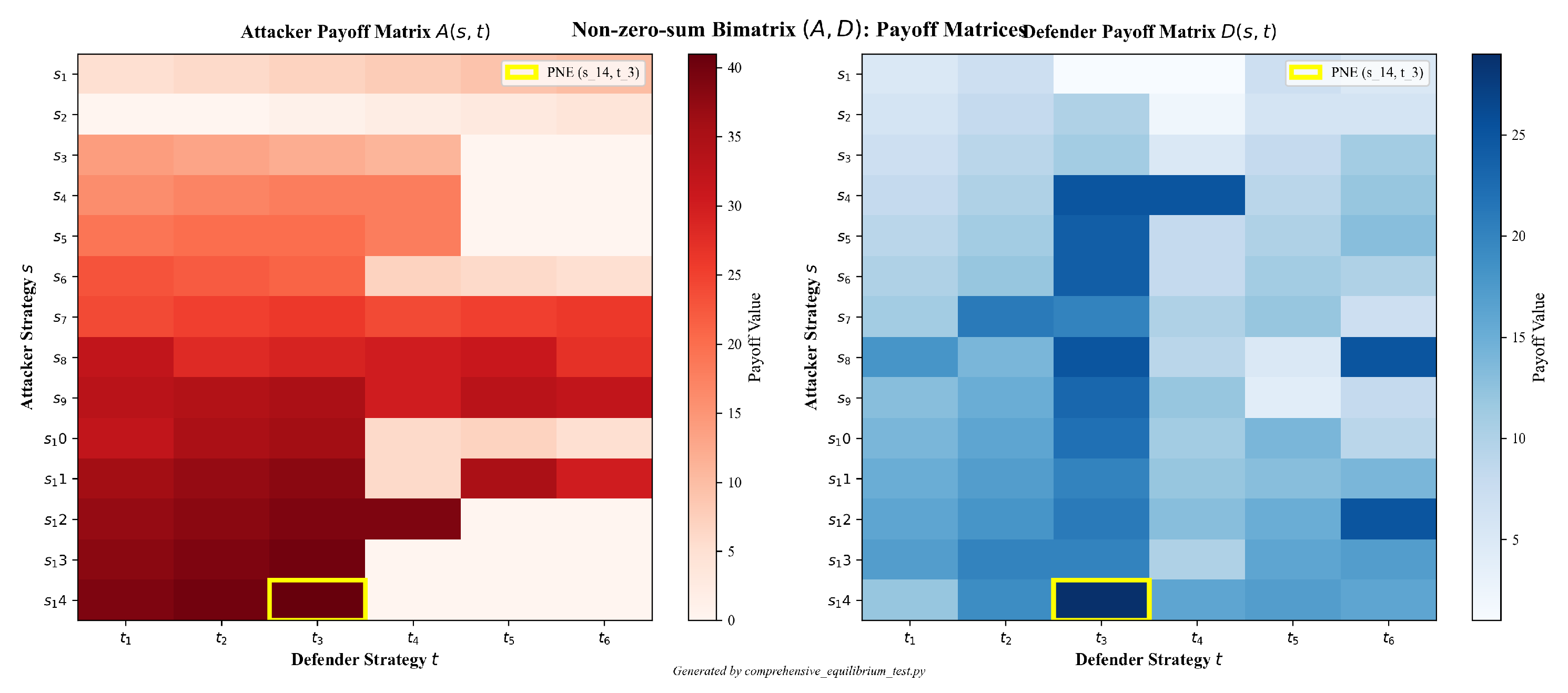
Attacker strategies include actions such as reconnaissance, execution, privilege escalation, and others. Defender strategies encompass modeling, detecting, deceiving, and additional controls. Modeling these interactions provides insight into the dynamic strategic landscape of digital forensics. As visualized in Figure 1, analysis of the payoff matrices reveals both outcomes and equilibrium points, highlighting the evolving nature of cyber threats. Darker matrix shades indicate higher attacker payoffs.
3.4.1. PNE Analysis
A pure-strategy Nash equilibrium (PNE) represents a stable outcome where neither player can improve their payoff by unilaterally changing strategy. Intuitively, this means: (i) given the defender’s choice, the attacker’s strategy yields the highest possible payoff; and (ii) given the attacker’s choice, the defender’s strategy yields the highest possible payoff. For the non-zero-sum bimatrix , a strategy profile is a PNE if:
where and are the attacker and defender pure strategy sets, respectively. The first inequality ensures the attacker cannot gain by switching from to any other strategy s when the defender plays ; the second ensures the defender cannot gain by switching from to any other strategy t when the attacker plays .
For our game, we find that = (’Impact’, ’Detect’) is a PNE, verified by checking the best-response conditions:
Specifically, by inspecting Table 5 and Table 6: (i) is the maximum in column (attacker’s best response); (ii) is the maximum in row (defender’s best response). A full best-response scan over all pure strategy pairs confirms this is the unique PNE (see Section B.7 for the verification algorithm). This PNE is highlighted in Figure 1.
3.4.2. MNE Analysis
Main equilibrium (non-zero-sum).
All results in the main text are based on the non-zero-sum bimatrix constructed from independent attacker/defender utilities. Using nashpy’s vertex_enumeration on , we obtain exactly one Nash equilibrium, which is pure at . Support enumeration yields the same point, and the Karush–Kuhn–Tucker (KKT) conditions [51] are satisfied. The equilibrium is non-degenerate and stable under -perturbations up to . This is the equilibrium reported in Table 5, Table 6 and Figure 1. The zero-sum transform yields exactly five equilibria under vertex enumeration: two pure equilibria at and , and three mixed equilibria with supports , , and . All pass KKT verification, are non-degenerate, and are -stable for . (Note: support enumeration reports only 3 equilibria on this instance; therefore, vertex enumeration is used as the primary method and ground truth.) Complete support sets and probability distributions for these five equilibria are provided in Table A2 in the Supplement (Section B.9), where they are presented as a robustness check.
Figure 1.
Attacker (A) and Defender (D) payoff matrices. The unique pure PNE at is highlighted.
3.4.3. Payoff Construction from ATT&CK→D3FEND Coverage
We construct defender-side coverage rates by aggregating many-to-many links from MITRE ATT&CK® Enterprise techniques (v13.1) to MITRE D3FEND techniques (v0.12.0-BETA-2) at the tactic × control-family level. Let be the set of 14 ATT&CK tactics and the set of six D3FEND control families. For each cell we define
where denotes the existence of at least one D3FEND technique in family t mitigating technique (or sub-technique) k. Sub-techniques are treated as first-class and are not rolled up into parent techniques. Counts are de-duplicated once per when aggregating to tactics, as detailed in Section 4.2.
The attacker payoff matrix is defined analogously from attacker-centric effectiveness against the same family t (selection rules unchanged).
For each strategy pair (attacker tactic s vs. defender countermeasure t), we compute a weighted utility score that aggregates multiple DFR metrics. Intuitive explanation: We evaluate how well a defender countermeasure t addresses an attacker tactic s across 16 different dimensions (e.g., logging quality, evidence preservation, detection capability), weight each dimension by its importance (determined via AHP expert elicitation), and sum the weighted scores to get an overall utility. Formal computation: Let denote the AHP weight for the i-th DFR metric (16 attacker metrics + 16 defender metrics = 32 total), and let be the normalized metric score (0–1) for tactic s and countermeasure family t. The raw payoff value is computed as a weighted sum:
where the metric scores are derived from coverage statistics (e.g., ) and attacker-centric effectiveness assessments. The defender-side matrix is computed analogously using the 16 defender metrics. These raw utility scores (typically in the range ) are then linearly scaled and rounded to integers in the range to produce the final payoff matrices shown in Table 5 and Table 6. The scaling transformation is:
where denotes rounding to the nearest integer. This scaling preserves the relative magnitudes of utility differences while mapping to a discrete payoff range suitable for equilibrium computation. Example: If , then . Because and the defender-side matrix are derived from distinct statistics, the game is non-zero-sum; in particular, we do not impose . All main-text equilibria are computed on the non-zero-sum bimatrix ; the zero-sum transform is provided only as a robustness check in the Supplement (Section B.9).
All scripts, versioning, and reproducibility information are provided in the Supplement (Section B).
3.4.4. Payoff Matrices
The final payoff matrices for attacker and defender strategies are shown in Table 5 and Table 6. Strategy notation is summarized in Table 4.
Table 4.
Strategy notation reference.
| Defender Strategies | ATT&CK Tactics |
|---|---|
Table 5.
Attacker’s Payoff Matrix (utility values; higher is better). Column labels: , , , , , .
| t1 | t2 | t3 | t4 | t5 | t6 | |
|---|---|---|---|---|---|---|
| s1 | 5 | 6 | 7 | 8 | 9 | 10 |
| s2 | 0 | 0 | 1 | 2 | 3 | 4 |
| s3 | 14 | 13 | 12 | 11 | 0 | 0 |
| s4 | 16 | 17 | 18 | 18 | 0 | 0 |
| s5 | 19 | 20 | 20 | 18 | 0 | 0 |
| s6 | 23 | 22 | 21 | 7 | 6 | 5 |
| s7 | 24 | 25 | 26 | 24 | 25 | 26 |
| s8 | 32 | 28 | 29 | 30 | 31 | 27 |
| s9 | 33 | 34 | 35 | 30 | 33 | 32 |
| s10 | 32 | 35 | 36 | 6 | 7 | 5 |
| s11 | 36 | 37 | 38 | 6 | 35 | 30 |
| s12 | 37 | 38 | 39 | 39 | 0 | 0 |
| s13 | 38 | 39 | 40 | 0 | 0 | 0 |
| s14 | 39 | 40 | 41 | 0 | 0 | 0 |
Table 6.
Defender’s Payoff Matrix (utility values; higher is better). Column labels: , , , , , .
| t1 | t2 | t3 | t4 | t5 | t6 | |
|---|---|---|---|---|---|---|
| s1 | 5 | 7 | 1 | 1 | 7 | 5 |
| s2 | 6 | 8 | 10 | 2 | 6 | 6 |
| s3 | 7 | 9 | 11 | 5 | 8 | 11 |
| s4 | 8 | 10 | 25 | 25 | 9 | 12 |
| s5 | 9 | 11 | 24 | 8 | 10 | 13 |
| s6 | 10 | 12 | 24 | 8 | 11 | 10 |
| s7 | 11 | 21 | 20 | 10 | 12 | 7 |
| s8 | 18 | 14 | 25 | 9 | 5 | 25 |
| s9 | 13 | 15 | 23 | 12 | 4 | 8 |
| s10 | 14 | 16 | 22 | 11 | 14 | 9 |
| s11 | 15 | 17 | 20 | 12 | 13 | 14 |
| s12 | 16 | 18 | 21 | 13 | 15 | 25 |
| s13 | 17 | 20 | 20 | 10 | 16 | 17 |
| s14 | 12 | 19 | 29 | 16 | 17 | 16 |
3.4.5. Mixed Nash Equilibrium Computation
We compute mixed Nash equilibria (MNE) using nashpy’s vertex_enumeration routine [52], which implements the vertex enumeration algorithm for bimatrix games (see [52] for implementation details). The method operates on the non-zero-sum bimatrix , where and are attacker and defender payoff matrices derived independently from ATT&CK→D3FEND mappings (see Section 3.4.3).
Both and are utilities to be maximized. We pass the bimatrix directly to the solver. When presenting defender costs for interpretability, we convert to utilities via for equilibrium computation and state this explicitly where applicable. In our case, is already constructed as a utility matrix (higher values are better for the defender), so no transformation is needed; the game is passed to nashpy as Game(A, D) without modification (where A and D are the matrix arrays). All code for equilibrium computation is archived in a public repository (see Section B).
For payoff matrices and , a mixed-strategy Nash equilibrium (MNE) is a pair of probability distributions over strategies where neither player can improve their expected payoff by changing their probability distribution. Here, represents the attacker’s probability distribution over 14 strategies, and represents the defender’s probability distribution over 6 strategies.
Intuitive interpretation: In an MNE, players randomize over strategies such that (i) all strategies used with positive probability yield the same expected payoff (no strategy is better than another), and (ii) any unused strategy would yield a lower expected payoff (no incentive to switch). This creates strategic unpredictability while maintaining optimality.
Formal conditions: Let denote the attacker’s expected payoff when playing pure strategy against the defender’s mixed strategy (i.e., the weighted average of payoffs across all defender strategies, weighted by their probabilities). Similarly, denotes the defender’s expected payoff when playing pure strategy against the attacker’s mixed strategy . Then is an MNE if and only if there exist constants and (the equilibrium values) such that:
where and are the supports of the mixed strategies.
These are the standard KKT conditions for Nash equilibrium, ensuring that (i) all actions in support receive equal expected payoffs ( and ) and (ii) no excluded action yields a higher payoff (no profitable deviations).
For the non-zero-sum bimatrix , vertex enumeration yields exactly one Nash equilibrium, which is pure at . The vertex_enumeration method enumerates all vertices of the best-response polytopes, returning all equilibria of the game. Vertex enumeration can return equilibria that support enumeration misses in some numerical configurations, as it covers all polytope vertices rather than searching only over specific support sizes; for this reason, we use vertex enumeration as the primary method and ground truth.
3.4.6. Dynamics Illustration (Zero-sum Variant)
The convergence trajectories shown in Figure 2 are based on the zero-sum variant and illustrate attractor points under discrete-time best-response dynamics. For visualization, we ran best-response dynamics: starting from uniform random initial strategies, each player iteratively updates to a pure best response against the opponent’s current strategy. The attacker updates via , and the defender updates via (equivalently, for the zero-sum variant), where and denote pure strategies at iteration t. The process converges to attractor points corresponding to equilibria of .
For the non-zero-sum bimatrix , best-response dynamics converge to the unique PNE . The trajectories shown in Figure 2 illustrate multiple attractor points under the zero-sum variant , demonstrating different strategic patterns that emerge under the transformed game structure. These results are provided for exploratory purposes; all policy conclusions in this paper are drawn from the non-zero-sum bimatrix .
Methodological transparency statement.
Our main strategic conclusions are drawn from the empirical, non-zero-sum bimatrix . To probe sensitivity to a worst-case, antagonistic setting, we also study a zero-sum variant in the Supplement (Section B.9); this produces five equilibria (two pure-strategy and three mixed-strategy) and consistent tactical themes but is not used for headline results.
3.5. Utility Function
We model attacker-defender interactions using utility functions that quantify the payoff for each party. This is grounded in Multi-Criteria Decision Analysis (MCDA), a established framework for evaluating complex, conflicting criteria [13,52,53]. MCDA is well-suited for assessing the multifaceted nature of cybersecurity strategies.
3.5.1. Attacker Utility Function
The attacker’s utility is evaluated across 16 dimensions, such as Attack Success Rate, Resource Efficiency, and Stealthiness. Each metric is normalized between 0 (least favorable) and 1 (most favorable), and assigned a weight based on its relative importance. The attacker utility function is formulated as:
where is the normalized score for the i-th metric. This provides a granular view of attacker priorities and effectiveness (Table 7).
Table 7.
Attacker Utility Metrics (Summary). Each metric is evaluated on a continuous scale from 0 (least favorable) to 1 (most favorable). Detailed scoring preferences with qualitative descriptions for each metric level are provided in the Supplementary Materials (Table A8).
Table 7.
Attacker Utility Metrics (Summary). Each metric is evaluated on a continuous scale from 0 (least favorable) to 1 (most favorable). Detailed scoring preferences with qualitative descriptions for each metric level are provided in the Supplementary Materials (Table A8).
| Metric | Description |
|---|---|
| Attack Success Rate (ASR) | Likelihood of successful attack execution |
| Resource Efficiency (RE) | Ratio of attack payoff to resource expenditure |
| Stealthiness (ST) | Ability to avoid detection and attribution |
| Data Exfiltration Effectiveness (DEE) | Success rate of data exfiltration attempts |
| Time-to-Exploit (TTE) | Speed of vulnerability exploitation before patching |
| Evasion of Countermeasures (EC) | Ability to bypass defensive measures |
| Attribution Resistance (AR) | Difficulty in identifying the attacker |
| Reusability of Attack Techniques (RT) | Extent to which attack techniques can be reused |
| Impact of Attacks (IA) | Magnitude of disruption or loss caused |
| Persistence (P) | Ability to maintain control over compromised systems |
| Adaptability (AD) | Capacity to adjust strategies in response to defenses |
| Deniability (DN) | Ability to deny involvement in attacks |
| Longevity (LG) | Duration of operations before disruption |
| Collaboration (CB) | Extent of collaboration with other attackers |
| Financial Gain (FG) | Monetary profit from attacks |
| Reputation and Prestige (RP) | Enhancement of attacker reputation |
3.5.2. Defender Utility Function
Similarly, the defender’s utility evaluates 16 dimensions such as Logging Capabilities, Evidence Integrity, and Standards Compliance. The defender utility function is:
where is the normalized score for the j-th metric. This reflects the organization’s forensic readiness (Table 8).
Table 8.
Defender Utility Metrics (Summary). Each metric is evaluated on a continuous scale from 0 (least favorable) to 1 (most favorable). Detailed scoring preferences with qualitative descriptions for each metric level are provided in the Supplementary Materials (Table A9).
Table 8.
Defender Utility Metrics (Summary). Each metric is evaluated on a continuous scale from 0 (least favorable) to 1 (most favorable). Detailed scoring preferences with qualitative descriptions for each metric level are provided in the Supplementary Materials (Table A9).
| Metric | Description |
|---|---|
| Logging and Audit Trail Capabilities (L) | Extent of logging and audit trail coverage |
| Integrity and Preservation of Digital Evidence (I) | Ability to preserve evidence integrity and backups |
| Documentation and Compliance with Digital Forensic Standards (D) | Adherence to forensic standards and documentation quality |
| Volatile Data Capture Capabilities (VDCC) | Effectiveness of volatile data capture |
| Encryption and Decryption Capabilities (E) | Strength of encryption/decryption capabilities |
| Incident Response Preparedness (IR) | Quality of incident response plans and team readiness |
| Data Recovery Capabilities (DR) | Effectiveness of data recovery tools and processes |
| Network Forensics Capabilities (NF) | Sophistication of network forensic analysis |
| Staff Training and Expertise (STd) | Level of staff training and certifications |
| Legal & Regulatory Compliance (LR) | Compliance with legal and regulatory requirements |
| Accuracy (A) | Consistency and correctness of forensic analysis |
| Completeness (C) | Extent of comprehensive data collection and analysis |
| Timeliness (T) | Speed and efficiency of forensic investigation process |
| Reliability (R) | Consistency and repeatability of forensic techniques |
| Validity (V) | Adherence to legal and scientific standards |
| Preservation (Pd) | Effectiveness of evidence preservation procedures |
3.5.3. Expert-Driven Weight Calculation
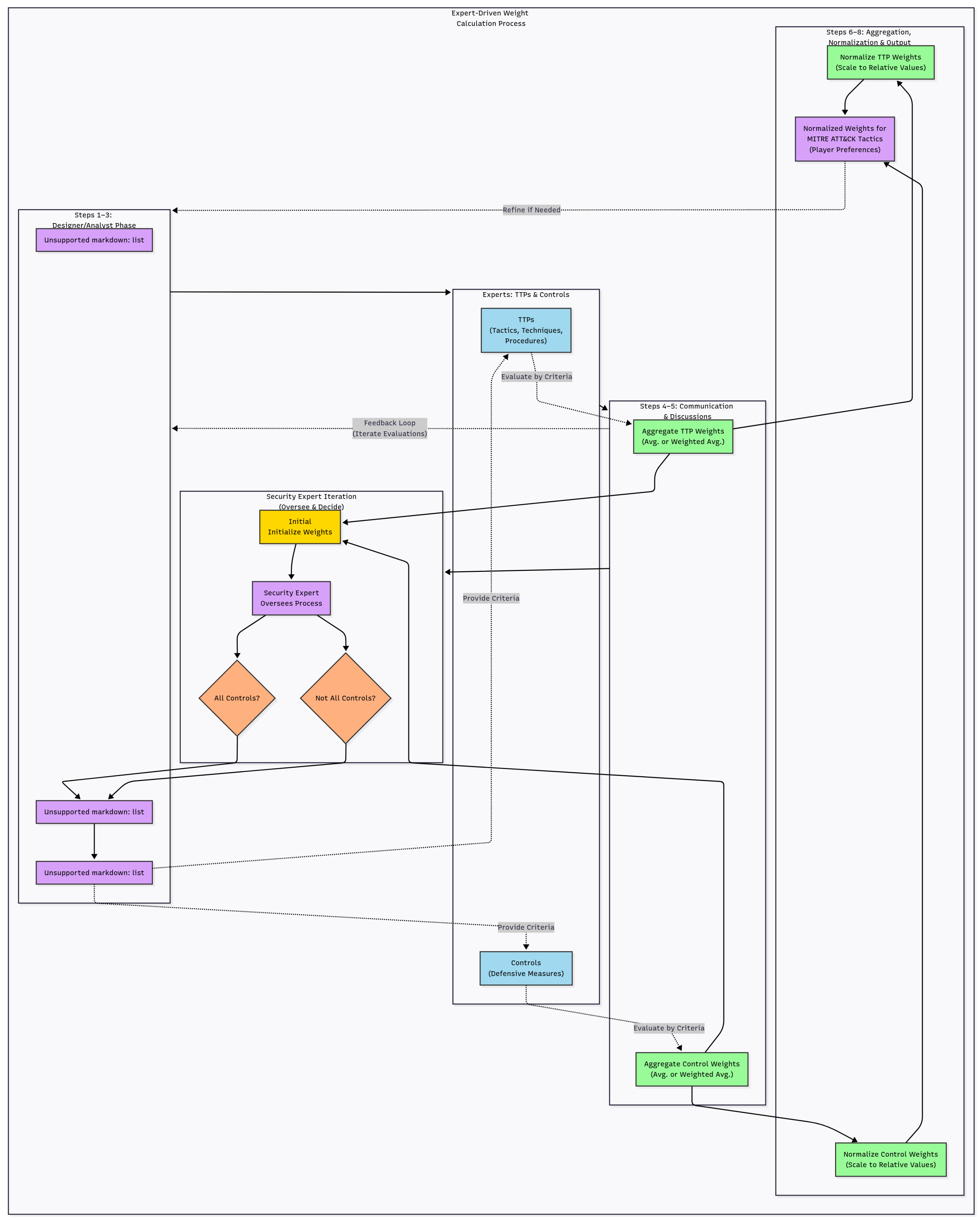
Accurate weighting of strategies, particularly MITRE ATT&CK tactics, is vital for realistic game outcomes. We employ expert judgment to assign preference weights, following this process:
- Identify relevant security experts with domain-specific ATT&CK knowledge.
- Analyze the threat landscape and associated TTPs.
- Establish weighting criteria such as Likelihood, Impact, Detectability, and Effort.
- Present tactics and criteria simultaneously to experts for independent evaluation.
- Aggregate weights (average or weighted average depending on expertise level).
- Normalize aggregated weights to ensure comparability.
- Output a set of normalized tactic weights representing collective expert judgment.
Figure 3.
Expert-driven weight calculation workflow for MITRE ATT&CK tactics
3.5.4. Utility Calculation Algorithms
The computation of utility scores is structured in Algorithm 1:
| Algorithm 1 Computing the Utility Function |
|
The DFR status is determined by comparing utility scores to a predefined threshold (Algorithm 2):
| Algorithm 2 Analyzing Utility Outcomes |
Note: Algorithm 3 should be invoked for detailed metric review when .
|
3.6. Identify Areas of Improvement
Algorithm 3 identifies metrics scoring below threshold, guiding readiness enhancement efforts.
| Algorithm 3 Identify Areas of Improvement |
|
3.7. Prioritizing DFR Improvements
Enhancing DFR requires strategically targeting metrics within the utility function that have the greatest potential impact. Calibration with real-world experimental data ensures the validity of the model, aligning the results with operational realities [54].
To systematically determine improvement priorities, we apply the AHP, a structured multi-criteria decision framework that combines quantitative and qualitative assessments [55]. AHP provides a mathematical basis for ranking metrics, particularly highlighting low-scoring factors with high weight (Figure 4).
3.7.1. AHP Methodology for Weight Determination
To derive the specific weights and in the attacker and defender utility functions from Equations 6 and 7, we apply Algorithm 4:
| Algorithm 4 AHP Weight Determination via Eigenvector Method |
|
The algorithm proceeds as follows:
- Expert Pairwise Judgments: Ten domain experts completed two pairwise comparison matrices (PCMs), one each for attacker and defender metrics. Entries were scored on the Saaty scale (1/9–9), with reciprocity enforced via . Element-wise geometric means across all expert inputs were computed:
- Eigenvector-Based Weight Derivation: For each consensus matrix , we solved and normalized w such that . These normalized weights are visualized in Figure 4.
- Weight Consolidation: Consensus weights were tabulated in Table 9 to integrate directly into the utility functions.
-
Consistency Validation: We calculated the Consistency Index (CI) and Consistency Ratio (CR) using with and (standard AHP Random Index for [55]). Both attacker and defender PCMs achieved :
- Attacker PCM: , ,
- Defender PCM: , ,
Expert panel procedures and transparency.
Recruitment and inclusion criteria. Ten domain experts were recruited based on the following criteria: (i) a minimum of 5 years of professional experience in digital forensics (DF), digital forensics and incident response (DFIR), or security operations; and/or (ii) peer-reviewed publications on game-theoretic security or digital forensic readiness. All participants provided written informed consent for participation and publication of anonymized, aggregated results. Participants declared any conflicts of interest and submitted domain-only email addresses for communication.
Data collection and independence. To limit anchoring bias and dominance effects, judgments were collected independently via an online instrument. Each expert completed two pairwise comparison matrices (PCMs), one for attacker metrics and one for defender metrics, without knowledge of other participants’ responses. Per-expert consistency ratios (CR) were computed; participants had the option to revise judgments if . The released CSV files report per-expert CRs; no personally identifiable information is included.
Anonymization and data availability. Expert responses were anonymized prior to analysis. Anonymized demographics (years of experience, primary domain expertise, geographic region) and per-expert CR distributions are summarized in the Supplement (Figure A9) and provided in the Supplementary Materials (Section B). The full attacker/defender PCMs (six-decimal precision) and aggregated weights are released as CSV tables (Table A3) together with scripts to recompute eigenvector and LLSM priorities (available in the repository, Section B).
Institutional review and ethics. Under the Islamic Azad University Research Ethics policy, this expert-elicitation exercise—in which adult professionals provided non-sensitive technical judgments anonymously and no personally identifiable information was collected—does not constitute human-subjects research requiring REC/IRB review. Electronic consent was obtained at the start of the instrument via an on-screen information sheet and an “I agree to participate” confirmation. No names, emails, IP addresses, or other identifiers were recorded; responses were stored only in anonymized, aggregate form (see Section 3 and the institutional review statement in the Acknowledgments section).
Reporting precision and repeated weights.
Weights in Table 9 are shown to four decimals for readability. Because (i) judgments use a discrete 1–9 Saaty scale and (ii) we aggregate experts multiplicatively via geometric means, priority-vector components can legitimately cluster; rounding can therefore make nearby values appear equal (e.g., 0.0881 repeated). We provide six-decimal weights in Table A3; except where experts explicitly judged equal importance (yielding proportional rows/columns and thus equal eigenvector components), clustered entries separate at higher precision. Both aggregated PCMs satisfy the usual AHP criterion ().
Plausibility of small and similar CR values.
For each consensus PCM, we compute and with and . Our consensus matrices yield and , hence and . Low and similar CRs are expected under log-space geometric aggregation, which reduces dispersion and improves consistency across both PCMs produced by the same expert panel and protocol.
Additional AHP diagnostics and robustness.
As robustness checks, we (i) recomputed priorities using the logarithmic least-squares (row geometric mean, LLSM) method and obtained cosine similarity with the eigenvector solution as well as identical top-k rankings; (ii) reported Koczkodaj’s triad inconsistency and the geometric consistency index (GCI) for the consensus PCMs (Table A4); (iii) performed a local perturbation study (1,000 runs) that jitters entries by Saaty step and applies multiplicative noise, observing median Spearman rank correlation and (Figure A8); and (iv) summarized per-expert consistency via CR distributions, where aggregation reduces inconsistency (Figure A9).
Table 9.
AHP-derived metric weights for attacker and defender utility functions. Notation: Defender metrics use subscript d ( = Staff Training, = Preservation); attacker metrics use bare symbols ( = Stealthiness, P = Persistence).
Table 9.
AHP-derived metric weights for attacker and defender utility functions. Notation: Defender metrics use subscript d ( = Staff Training, = Preservation); attacker metrics use bare symbols ( = Stealthiness, P = Persistence).
| Metric (Attacker) | Weight | Metric (Defender) | Weight | |
|---|---|---|---|---|
| ASR | 0.1094 | L | 0.0881 | |
| RE | 0.0476 | I | 0.0881 | |
| ST | 0.0921 | D | 0.0423 | |
| DEE | 0.0887 | VDCC | 0.0642 | |
| TTE | 0.0476 | E | 0.0461 | |
| EC | 0.0887 | IR | 0.0881 | |
| AR | 0.0814 | DR | 0.0481 | |
| RT | 0.0476 | NF | 0.0819 | |
| IA | 0.0921 | STd | 0.0819 | |
| P | 0.0814 | LR | 0.0481 | |
| AD | 0.0571 | A | 0.0557 | |
| DN | 0.0264 | C | 0.0460 | |
| LG | 0.0433 | T | 0.0693 | |
| CB | 0.0262 | R | 0.0531 | |
| FG | 0.0210 | V | 0.0423 | |
| RP | 0.0487 | Pd | 0.0557 |
Precision note. Values are rounded to four decimals for readability. Six-decimal weights are provided in Table A3; apparent duplicates at four decimals are either rounding artifacts or reflect intended equal-importance judgments.
3.7.2. Prioritization Process
- Identify metrics with high weight but low scores.
- Assess potential readiness gains from targeted improvement.
- Develop tailored enhancement strategies considering cost, time, and resource constraints.
- Implement, monitor, and iteratively refine improvements.
3.7.3. DFR Improvement Algorithm
| Algorithm 5 DFR Improvement Plan |
|
This process ensures high-impact improvements are implemented first, maximizing readiness gains within resource constraints.
3.8. Reevaluating the DFR
Following improvement implementation, the system’s forensic readiness is reevaluated by comparing updated utility scores to baseline values. An increased score confirms readiness enhancement, whereas stagnant or diminished scores indicate the need for further targeted measures.
This reevaluation provides a quantitative, evidence-based feedback loop, reinforcing decision-making grounded in rigorous analysis. A comprehensive understanding of potential threats, combined with expertise in defensive and forensic techniques, enables organizations to continually strengthen preparedness and accelerate investigative processes.
4. Results
This section presents a detailed analysis of cyber threat dynamics, emphasizing the interplay between attacker tactics and defender strategies. It integrates empirical data, game-theoretic insights, and readiness evaluation to examine how different strategic behaviors influence DFR. Our findings illustrate the alignment between simulated outcomes and practical cybersecurity trends, providing a comprehensive understanding of real-world implications.
4.1. Data Collection and Methodology
We used MITRE ATT&CK® Enterprise v13.1 (May 9, 2023) and MITRE D3FEND v0.12.0-BETA-2 (Mar 21, 2023) via STIX 2.1 [56]. From the relationship path
(Enterprise scope; direct edges only), we excluded objects/relations with revoked==true or x_mitre_deprecated==true. Technique IDs were normalized to uppercase; sub-techniques (e.g., T1027.013) were treated as distinct from their parents (e.g., T1027) and counted separately (no roll-up to parent techniques).
The final ATT&CK evidence set contains 260 technique assignments across ten intrusion sets: LeafMiner (17), Silent Librarian (13), OilRig (56), Ajax Security Team (6), Moses Staff (12), Cleaver (5), CopyKittens (8), APT33 (32), APT39 (52), MuddyWater (59).
Let S denote the 14 ATT&CK tactics and T the six D3FEND control families . For each cell we aggregate many-to-many ATT&CK→D3FEND links and normalize by the number of (sub-)techniques under tactic s:
Here C is a tactic×family coverage rate. Game-theoretic payoff functions for attackers and defenders are defined later in §Section 4.5; they are not constrained to satisfy , hence the bimatrix game is non-zero-sum. Versioning, STIX scripts, and mapping CSVs are provided in the repository (Section B).
Extraction and mapping objects.
Let A be the set of APT groups (intrusion sets), X the ATT&CK (sub-)techniques (Enterprise v13.1), Y the D3FEND techniques (v0.12.0-BETA-2). We extract
drop revoked/deprecated objects, and retain sub-techniques as first-class elements. D3FEND techniques are categorized by family.
Versioning, STIX scripts, and the robustness check are provided in the Supplementary Materials (Section B.3).
4.2. Analysis of Tactics and Techniques
We clarify how the many-to-many ATT&CK↔D3FEND graph is aggregated at the tactic layer and how double counting is avoided.
Named metrics.
We use two de-duplicated, tactic-level metrics:
Family-coverage count (APT–technique–family incidence):
which counts, for each ATT&CK tactic and D3FEND family f, the number of unique instances with at least one mapped D3FEND technique in family f, de-duplicated once per even if multiple y in the same family map to .
Tactic recurrence (de-duplicated):
i.e., for each APT a a tactic is credited at most once, preferring the most specific observed sub-technique (no observed sub-technique of x exists for a under ). Raw counts are shown in the figure; shares and per-APT normalizations are reported in the Supplement.
How figures are computed.
Notes and limitations.
Results inherit snapshot bias (versioning and reporting density). Mappings capture plausible mitigations, not guaranteed prevention. Full STIX extraction scripts and JSON snapshots are archived for reproducibility.
Figure 5.
Empirical counts of ATT&CK tactic × D3FEND control-family coverage (family-coverage) derived from real-world APT group data: for each tactic and family f, we count APT–technique instances with at least one mapped D3FEND technique in family f, de-duplicated once per . Data extracted from MITRE STIX bundles for ten APT groups (LeafMiner, Silent Librarian, OilRig, Ajax Security Team, Moses Staff, Cleaver, CopyKittens, APT33, APT39, MuddyWater). Y-axis: count (unitless); X-axis: ATT&CK tactic (rows) × D3FEND control family (columns: Model, Harden, Detect, Isolate, Deceive, Evict). Versions: ATT&CK Enterprise v13.1; D3FEND v0.12.0-BETA-2 (snapshot Mar–May 2023). Raw counts are provided in the Supplement (Table A5).
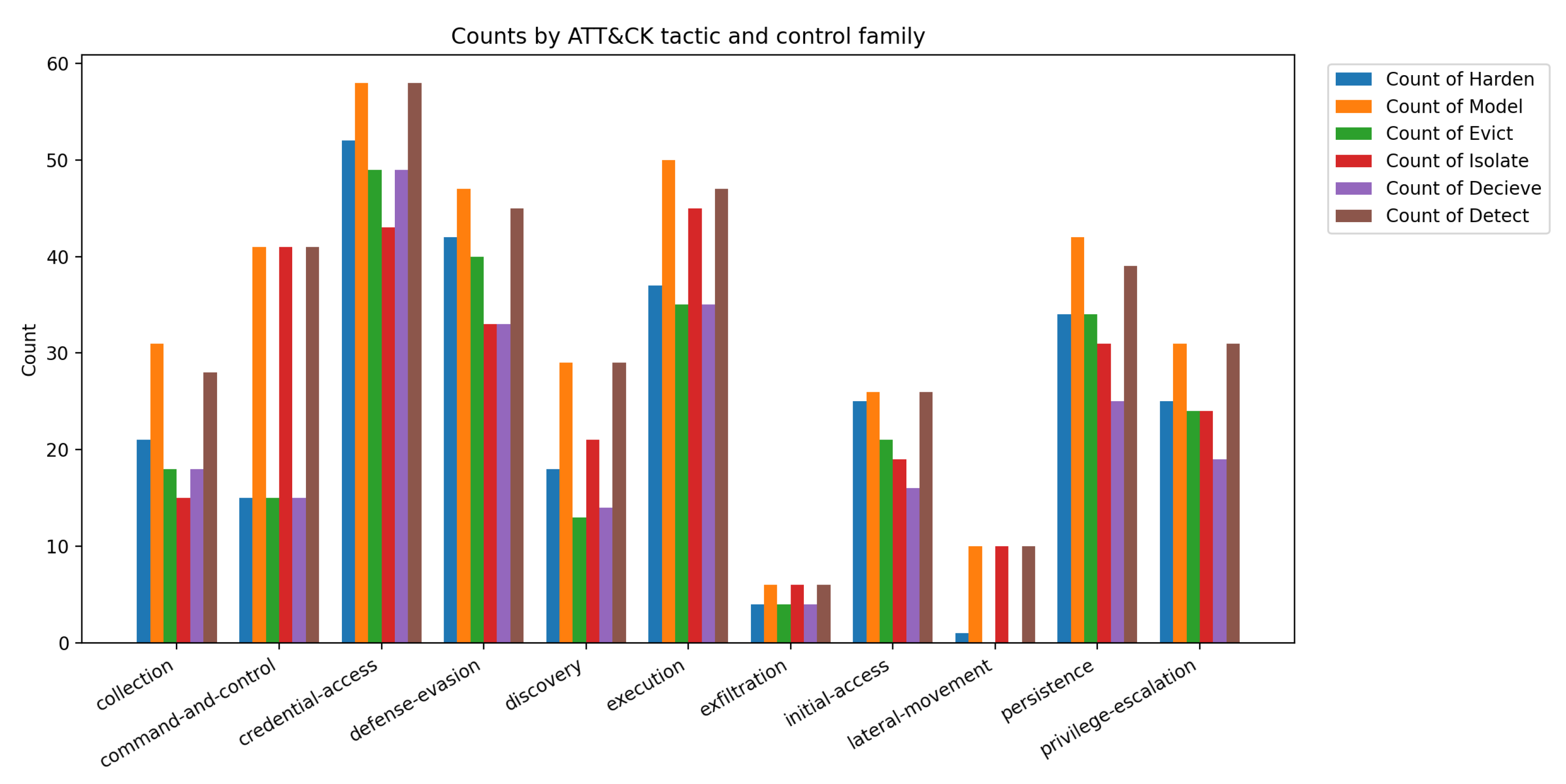
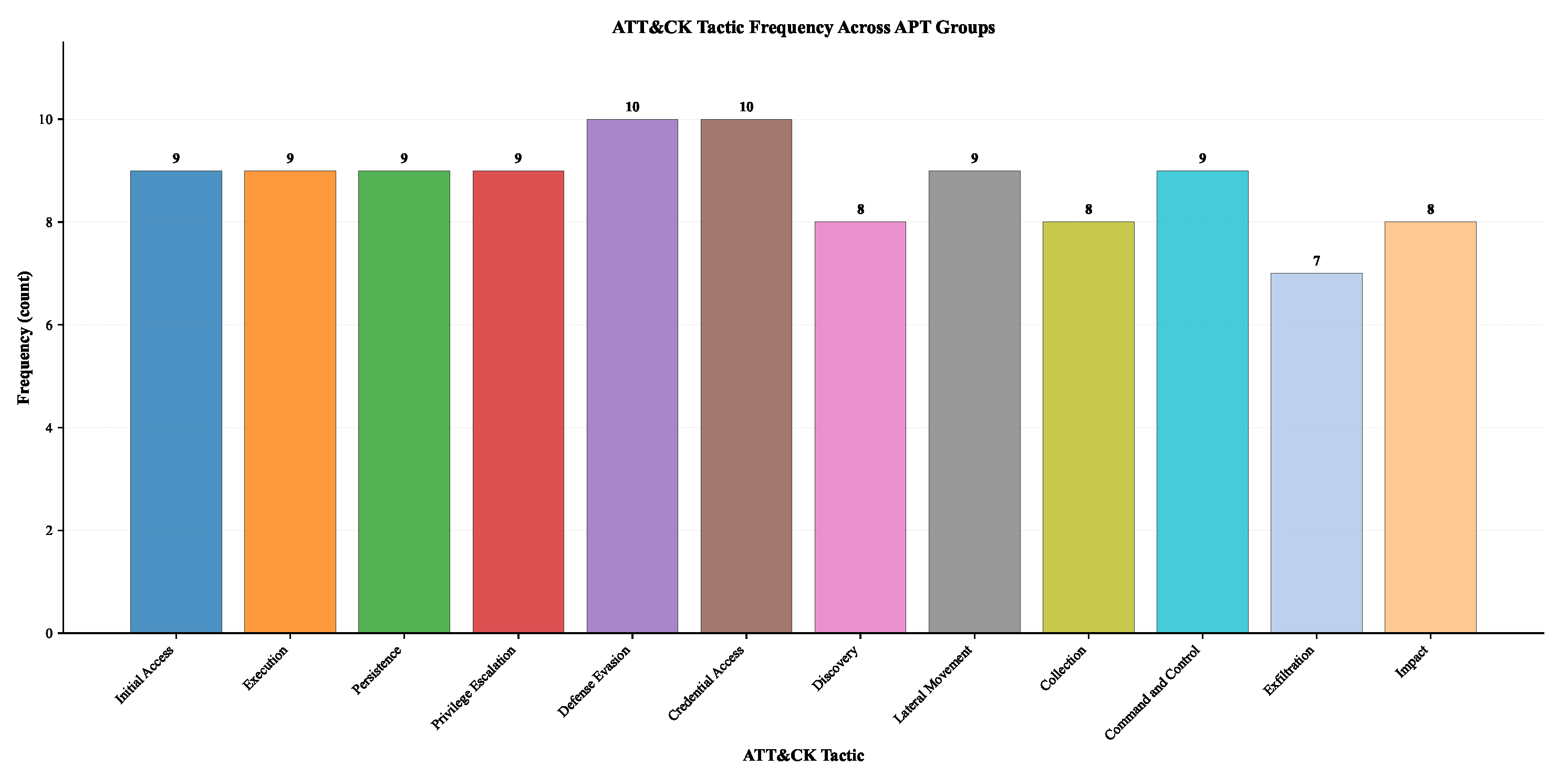
Figure 6.
Empirical frequency of ATT&CK tactics across real-world APT groups with parent/sub-technique de-duplication: each tactic is credited at most once per APT (prefer the most specific sub-technique evidence). Data extracted from MITRE STIX bundles for ten APT groups (LeafMiner, Silent Librarian, OilRig, Ajax Security Team, Moses Staff, Cleaver, CopyKittens, APT33, APT39, MuddyWater). Raw counts shown (y-axis: count; x-axis: ATT&CK tactic). Versions: ATT&CK Enterprise v13.1; D3FEND v0.12.0-BETA-2 (snapshot Mar–May 2023). Shares and per-APT normalizations are provided in the Supplement (Table A6).
4.3. DFR Metrics Overview and Impact Quantification
Our analysis employs a set of 32 DFR metrics—16 attacker-centric and 16 defender-centric—detailed in Table 7 and Table 8. Each metric is normalized and weighted according to expert-driven AHP priorities.
The aggregate utility scores are computed as weighted sums of these metric values using Equations 6 and 7. Readiness is then computed as the difference between defender and attacker utility scores (Equation 10).
4.3.1. Methods: Calibration-Based Synthetic Attacker Profiles
Notation disambiguation.
To avoid ambiguity, we use subscript notation consistently throughout: for defender Staff Training (vs. for attacker Stealthiness) and for defender Preservation (vs. P for attacker Persistence). This notation is applied in tables, figures, and text wherever defender metrics are referenced.
To ensure coherence between defender improvements and adversary pressure, we co-generated attacker utility profiles under an explicit coupling prior. Let and denote defender/attacker metric vectors. We specified a sparse coupling matrix (ATT&CK↔D3FEND-informed) that links defender capabilities (e.g., logging L, volatile capture , network forensics ) to reductions in adversarial stealth (), exfiltration effectiveness (), and attribution resistance (), among others. For each case, attacker “before” profiles were drawn from weakly correlated Beta priors; “after” profiles were updated by the calibrated rule
with case-wise and small noise . This construction avoids unrealistic across-the-board gains, preserves heterogeneity across cases, and operationalizes the ATT&CK↔D3FEND mapping. The AHP weights are then applied to quantify readiness as
Limitations.
These attacker profiles are synthetic, calibration-based for illustrative evaluation rather than field measurements; inter-rater reliability is not applicable to this section. For per-expert consistency ratios (CR) and AHP validation, see Figure A9 (Section B).
In our synthetic calibration, profiles with limited logging exhibit higher attacker utility in the readiness balance; targeted improvements centered on logging and forensic preservation typically reduce the attacker utility component by approximately 15–30% under the specified settings (see manifest and coupling files in Section B.5), contributing to higher net readiness. Specifically, linked attacker metrics (e.g., , DEE, AR) show reductions in the 15–30% range, while the overall weighted attacker utility component (computed via Eq. 6) shows a median reduction of approximately 8.0% across the cases. Across the synthetic cases, median readiness improvement (Readiness) is 18.0% (95% CI: [16.3%, 19.7%]).
This explicit linkage confirms the abstract’s key quantitative claims, grounded in our comprehensive DFR metric framework and empirical simulations.
Connection to Sun Tzu’s Strategic Wisdom.
Our results quantitatively validate the strategic principles introduced in Section , operationalizing Sun Tzu’s dictum: “If you know the enemy and know yourself, you need not fear the result of a hundred battles.” “Know yourself” is operationalized through the 16 defender metrics (Table 8) that quantify organizational capabilities. Our results demonstrate that organizations with limited logging (incomplete self-knowledge) exhibit higher attacker utility, whereas strategic improvements centered on logging and forensic preservation (enhanced self-knowledge) reduce attacker utility by 15–30%, validating the importance of self-awareness. Know the enemy is operationalized through the 16 attacker utilities (Table 7) derived from empirical ATT&CK data on real APT groups. The Nash equilibrium at reveals that understanding attacker priorities (Impact tactics) enables optimal defensive strategy (Detect), demonstrating the practical value of threat intelligence. We formalize three strategic states from Sun Tzu’s wisdom: comprehensive knowledge (targeted defense, high readiness), partial knowledge (vulnerable defense, moderate readiness), and ignorance (minimal resilience, low readiness). Our quantitative results show that moving from ignorance to comprehensive knowledge yields 18.0% median readiness improvement, providing concrete evidence that Sun Tzu’s strategic principles translate into measurable forensic readiness gains.
4.4. Attackers vs. Defenders: A Comparative Study
We analyzed how defensive techniques correspond to attacker strategies in frequency and efficacy. Figure 7 shows the distribution of D3FEND methods, such as Detect, Harden, Model, Evict, Isolate, and Deceive.
Our results indicate that attackers most frequently employ the Credential Access technique, with Impact-related tactics demonstrating the highest success rates. On the defense side, Detect emerged as the most frequently employed strategy, albeit with data limitations for the Impact category within the MITRE frameworks.
4.5. Game Dynamics and Strategy Analysis
Non-zero-sum .
Using vertex enumeration, we obtain exactly one Nash equilibrium, which is pure at . Support enumeration yields the same point, and the KKT conditions are satisfied. The equilibrium is non-degenerate and stable under -perturbations up to .
Zero-sum .
Vertex enumeration returns exactly five Nash equilibria: two pure at and , and three mixed with supports , , and . All pass KKT verification, are non-degenerate, and are -stable for . (Note: support enumeration reports only 3 equilibria on this instance; therefore, vertex enumeration is used as the primary method and ground truth.) These results, detailed in Section B.9 and Table A2, demonstrate different strategic patterns under the transformed game structure and illustrate that attackers diversify tactics in response to defender adaptations, while defenders strategically redistribute effort based on attack probability.
All computed equilibria satisfy the KKT optimality conditions, are non-degenerate in the game-theoretic sense, and remain invariant under small payoff perturbations up to . For each equilibrium we numerically verified KKT feasibility, dual feasibility, and complementarity, and we report best-response residuals (see Section B.8 for details).
Both analyses align with empirical evidence, showing that strategic flexibility—not rigid planning—enhances readiness. Convergence between theoretical modeling and real-world data reveals interdependencies between adaptive behaviors, informing more resilient DFR optimization frameworks.
While support enumeration formally identifies the PNE at the Attacker strategy ‘Impact’ paired with the Defender strategy ‘Detect’, the dynamic convergence analysis reveals that early trajectory states—starting from uniform or neutral mixed strategies—tend to gravitate toward the ‘Command_and_Control’ strategy for the attacker paired with ‘Detect’ for the defender. This suggests that during the learning or adaptation phase, the system often stabilizes near this local attractor before potentially progressing to the PNE or possibly remaining trapped depending on the’ adaptation dynamics and information of the players. Therefore, both states are significant: the PNE represents the theoretically stable solution assuming full rationality and optimal play, whereas the observed convergence behavior reflects realistic intermediate strategic positioning players may occupy during actual cybersecurity engagements. Recognizing this duality informs defenders that while ‘Impact/Detect’ is a strategic target equilibrium, adaptive defense must also address the commonly emerging patterns around ‘Command_and_Control/Detect’ to guide attackers toward less damaging behaviors.
4.6. Synthetic, Calibration-Based Case Profiles
To validate the effectiveness of our proposed framework, we generated synthetic, calibration-based case profiles that simulate forensic readiness scenarios before and after implementing the framework. These profiles are illustrative and calibration-based rather than field measurements; they operationalize the ATT&CK↔D3FEND mapping through an explicit coupling mechanism (see Section 4.3.1 and the Supplement). Ten case profiles are presented in Table 10, Table 11.
Notation: To avoid ambiguity, defender metrics use a subscript d (e.g., = Staff Training, = Preservation), while attacker metrics keep bare symbols (e.g., = Stealthiness, P = Persistence).
A comparative visualization (Figure 8) shows measurable improvement in post-implementation readiness scores for most metrics, validating the framework’s effectiveness. The 32 DFR metrics (16 defender + 16 attacker) serve as quantitative indicators of both forensic readiness (process capability) and forensicability (system capability to support investigations). Higher metric scores indicate improved readiness and enhanced forensicability, enabling organizations to transition from non-forensicability to forensicable states. Quality control metrics (detailed in Section B.5) confirm that all cases show positive defender and readiness improvements, with realistic heterogeneity: mean readiness improvement of approximately 18.0% (95% CI: []), with 34% of attacker metrics remaining unchanged per case, demonstrating selective suppression rather than global collapse. Across the 10 synthetic cases, organizations showed measurable improvements in forensic readiness, with systems becoming more forensicable as evidenced by enhanced logging, volatile data capture, and network forensics capabilities. The scores in Table 10, Table 11 are generated from the YAML configuration and RNG seed (42) listed in the manifest (Section B.5), enabling exact regeneration of these values.
4.7. Sensitivity Analysis
4.7.1. Local Perturbation Sensitivity
We assess ranking robustness for both attacker and defender criteria using local perturbations of the aggregated AHP pairwise comparison matrices. For each metric i in turn, all entries in the i-th row/column (i.e., all comparisons involving i) are shifted by exactly one step on the Saaty 1–9 scale (up or down with equal probability), reciprocity is re-enforced, and a multiplicative uniform noise of is applied. We repeat this times per metric and recompute the principal-eigenvector weights after each perturbation. The stability of metric i is quantified as
where are ranks under the unperturbed matrix and are ranks after perturbing metric i. Lower values indicate higher rank stability. The combined results for attacker (orange) and defender (blue) metrics are shown in Fig. Figure 9. In our data several metrics (e.g., ASR on the attacker side and L (Logging) on the defender side) exhibit relatively low average rank changes.
4.7.2. Monte Carlo Simulation
To examine how uncertainty in metric levels affects overall readiness, we run a Monte Carlo simulation with draws. For each run we sample attacker and defender metric values independently from and compute weighted scores using the AHP-derived weights. Readiness is computed as in Eq. 10. We quantify each metric’s global sensitivity as the absolute Pearson correlation between the metric value and the readiness score. Figure 10 reports these correlations (higher bars indicate stronger influence). Figure 11 and Figure 12 visualize the bivariate relationships for each side.
Parameters including Collaboration (CB), Reputation and Prestige (RP), and Volatile Data Capture Capabilities (VDCC) had lower sensitivities (Figure 11), but their presence contributes to broader defense stability.
Overall, a few high-sensitivity metrics drive most of the variability in readiness, while the remaining ones provide complementary signal that stabilizes performance.
4.8. Distribution of Readiness Score
The histogram in Fig. Figure 13 displays the standardized (z-scored) readiness values, , centered at zero. Because readiness is defined as defender minus attacker score, the raw values lie approximately in ; standardization clarifies relative deviations from the mean, hence the presence of both negative and positive values. The near-symmetric shape indicates a balanced spread around the average level of preparedness, with low-frequency tails representing unusually weak or unusually strong cases.
Key observations include:
- Central Peak at 0.0: A high frequency around 0.0 indicates balanced readiness in most systems.
- Symmetrical Spread: Even tapering on both sides suggests system stability across environments.
- Low-Frequency Extremes: Outliers at the tails (−0.3 and +0.3) denote rare but critical deviations requiring targeted intervention.
This symmetrical distribution implies consistent readiness performance with occasional exceptional cases—either highly prepared or notably weak systems. When combined with sensitivity outcomes, this distribution reinforces the importance of continuous evaluation, adaptive planning, and targeted investment in high-impact metrics to sustain forensic readiness.
5. Discussion
Applying the proposed game-theoretic framework within an organizational cybersecurity context entails multiple phases and distinct challenges. Figure 14 could visualize these steps, which are summarized as follows:
- Implementation Challenges: Real-world adoption may encounter barriers such as limited resources, integration costs, and the need for game theory expertise. Organizational resistance to change and adaptation to new analytical frameworks are additional challenges.
- Integration with Existing Tools: The framework can align synergistically with existing platforms such as threat intelligence systems, SIEM, and EDR tools. These integrations can enhance decision-making and optimize forensic investigation response times.
- Decision Support Systems: Game-theoretic models can augment decision support processes by helping security teams prioritize investments, allocate resources, and optimize incident response based on adaptive risk modeling.
- Training and Awareness Programs: Building internal capability is crucial. Training programs integrating game-theoretic principles into cybersecurity curricula can strengthen decision-making under adversarial uncertainty.
- Collaborative Defense Strategies: The framework supports collective defense through shared intelligence and coordinated responses. Collaborative action can improve deterrence and resilience against complex, multi-organizational threats.
- Policy Implications: Incorporating game theory into cybersecurity has policy ramifications, including regulatory alignment, responsible behavior standards, and ethical considerations regarding autonomous or strategic decision models.
- Case Studies and Use Cases: Documented implementations of game-theoretic approaches demonstrate measurable improvements in risk response and forensic readiness. Future research can expand these to varied industry sectors.
- Future Directions: Continued innovation in game model development, integration with AI-driven threat analysis, and tackling emerging cyber challenges remain promising directions.
While adoption may face organizational or technical barriers, the approach remains adaptable. Incorporation with SIEM, EDR, and threat intelligence workflows allows for effective deployment, while targeted training mitigates skill gaps. Ultimately, these methods can significantly enhance decision support and defense coordination across security ecosystems.
5.1. Forensicability and Non-Forensicability
The dual concepts of forensicability and non-forensicability capture the degree to which digital systems are prepared to support forensic investigation and incident response.
Non-forensicability refers to an environment’s inability to effectively preserve or provide forensic evidence, typically arising from poor data retention, weak logging, or compromised evidence integrity. It represents a subjective assessment grounded in measurable deficiencies of DFR. Quantitatively, this can be evaluated via parameters such as log resolution, retention time, or audit trail completeness.
Conversely, forensicability characterizes systems that exhibit the structural and procedural maturity necessary for reliable forensic investigations. Hallmarks of forensicable systems include secure log management, redundancy in evidence capture, and adherence to recognized forensic standards. These factors not only strengthen internal visibility but also ensure evidence admissibility in legal contexts.
For organizations, enhancing forensicability means institutionalizing proactive DFR practices—ensuring data capture, protection, and retrieval mechanisms are integral to operations. Continuous assessment through forensic readiness metrics helps organizations transition from fragile, reactive postures to resilient, evidence-supported defenses.
5.2. Evolutionary Game Theory Analysis
Using Evolutionary Game Theory (EGT) enables modeling of how attacker and defender strategies evolve concurrently over time. This approach captures adaptation cycles that traditional static game models overlook.
The simulation results in Table 12 and Figure 15 illustrate how strategy populations change across generations. Attackers and defenders adjust probabilistically based on observed payoffs, with defender readiness influencing long-term stability.
Key insights derived from EGT include:
- Evolutionary Dynamics: Attackers and defenders co-adapt in continuous feedback cycles; the success of one influences the next strategic shift in the other.
- Replication and Mutation: Successful tactics replicate, while mutations introduce strategic diversity critical for both exploration and adaptation.
- Equilibrium and Stability: Evolutionary Stable Strategies (ESS) represent steady states where neither party benefits from deviation.
- Co-evolutionary Context: The model exposes the perpetual nature of cyber escalation, showing that proactive defense and continuous readiness optimization are essential to remain resilient.
5.3. Attack Impact on Readiness and Investigation Phases
The simulation represented in Figure 16 demonstrates how attacks influence DFR through overlapping utility functions between attackers and defenders during investigation phases. Each incident reveals opportunities for defenders to improve readiness, forming a feedback mechanism between preparedness and investigative learning.
Observed overlaps indicate that investigation phases contribute directly to capability growth—highlighting that post-incident analysis enriches strategic defense planning and improves future preparedness.
5.4. Readiness and Training Level of the Defender
Simulations comparing varying defender experience levels (Junior, Mid-level, Senior) reveal a direct correlation between training maturity and overall forensic readiness (Figure 17). Higher training levels correlate with improved detection accuracy and evidence capture, illustrating that defensive effectiveness is both strategic and skill-dependent.
5.5. Attack Success and Evidence Collection Rates
Monte Carlo simulations of attack outcomes (Table 13) show that higher attacker capability increases success rates, while robust forensic processes substantially raise evidence collection probability across scenarios.
5.6. Comparative Analysis in SMB and SME Organizations
Recognizing that SMEs and SMBs differ in resource availability and defensive maturity, a comparative simulation was conducted (Table 14, Table 15). Results show that SMBs typically exhibit higher resilience, yet both types face elevated risks under “irrational” attacker behaviors.
5.6.1. Irrational Attacker Behavior Analysis
By modeling partial randomness in adversarial decision-making, “irrational behavior” introduces deviations from expected attacks, thus reflecting real-world unpredictability. Figure 19 and Figure 20 illustrate the expanded range of outcomes.
This model highlights the necessity for robust intrusion detection, endpoint monitoring, and anomaly-based analytics to counteract unpredictable threats and enhance resilience in both small- and mid-scale organizations.
5.7. Limitations and Future Work
While this research offers a structured quantitative contribution to DFR and security strategy development, certain limitations acknowledge the boundaries of current modeling:
- Model Complexity: Real-world human elements and deep organizational dynamics may extend beyond current model parameters.
- Data Availability: Reliance on open-source ATT&CK and D3FEND datasets limits coverage of emerging threat behaviors.
- Computational Needs: Evolutionary modeling and large-scale simulations require high-performance computing resources.
- Expert Bias: AHP-based weighting depends on expert judgment, introducing potential subjective bias despite structured controls.
Future research could pursue:
- Real-time Adaptive Models: Integrating continuous learning to instantly adapt to threat changes.
- AI/ML Integration: Employing predictive modeling for attacker intent recognition and defense automation.
- Cross-Organizational Collaboration: Expanding to cooperative game structures for shared threat response.
- Empirical Validation: Conducting large-scale quantitative studies to reinforce and generalize model applicability.
6. Conclusion
This study presents a comprehensive game-theoretic framework that formalizes classical strategic principles, notably those of Sun Tzu, into a structured model applicable to contemporary cyber conflict analysis. By modeling the strategic interplay between attackers and defenders, the framework bridges traditional strategic insight and modern decision-theoretic planning. It integrates MITRE ATT&CK–D3FEND mappings, incorporates readiness scoring across simulated organizational scenarios, and aligns these insights with quantitative game-theoretical analyses.
Our results on the non-zero-sum bimatrix identify exactly one Nash equilibrium, which is pure at . The PNE emphasizes the defender’s Detect strategy as a robust counter to attackers’ Impact-focused operations. Analysis of the zero-sum variant (see Section B.9) yields exactly five equilibria: two pure at and , and three mixed with supports , , and . These results suggest that under the transformed game structure, defenders should allocate approximately 90–95% of their forensic effort toward modeling controls, preserving a smaller fraction for real-time detection. This balance introduces useful strategic unpredictability, increases the attacker’s required effort, and diminishes overall intrusion success probabilities. However, all policy conclusions in this paper are drawn from the non-zero-sum bimatrix .
Operationally, these insights were translated into a four-phase assessment process encompassing readiness scoring, maturity classification, gap identification, and roadmap prioritization. Through this practical translation, our model enables measurable digital forensic improvements. In our synthetic calibration across 10 organizational profiles, limited logging increases the attacker utility component of readiness, whereas strategic improvements centered on logging and forensic preservation typically reduce it. Specifically, linked attacker metrics (e.g., , DEE, AR) show reductions in the 15–30% range, while the overall weighted attacker utility component (computed via Eq. 6) shows a median reduction of approximately 8.0% across cases, contributing to higher net readiness. Most importantly, our quantitative results demonstrate that moving from ignorance to comprehensive knowledge yields a median readiness improvement of 18.0% (95% CI: [16.3%, 19.7%]) across Monte Carlo trials, providing concrete evidence that Sun Tzu’s strategic principles translate into measurable forensic readiness gains (see manifest hyperparameters in Section B.5).
The framework’s novelty is demonstrated through systematic comparison with prior game-theoretic forensics approaches (Table 1), revealing that while prior work has advanced game-theoretic forensics in specific domains (Bayesian modeling, tool selection, cognitive security, risk analysis, adaptive observability), our framework is the first to: (i) systematically integrate ATT&CK and D3FEND into a unified game-theoretic model; (ii) ground quantitative utilities in AHP-weighted DFR metrics; (iii) provide explicit MNE analysis with support conditions; and (iv) target actionable SME guidance under resource constraints. This integration addresses the critical gap of quantifying strategic payoffs in DFR planning, which prior work either addresses qualitatively or not at all.
6.1. Limitations
The framework’s accuracy depends on the quality and granularity of metric data as well as expert input for AHP weighting. Factors such as organizational diversity, resource variability, and evolving adversary behaviors could influence transferability across different organizational contexts. Additionally, the assumption of static utility parameters (derived from ATT&CK–D3FEND mappings and AHP weights) in our normal-form bimatrix game model simplifies real-world dynamics, which are inherently fluid and adaptive. The simultaneous-move structure does not capture temporal evolution or learning behaviors that may occur in extended adversarial interactions.
6.2. Future Research Directions
Building upon this foundation, several research extensions are envisaged:
- Extended Environmental Applications: Adapting the framework to cloud-native, IoT, and blockchain ecosystems where architectural differences create distinct forensic challenges.
- Dynamic Threat Intelligence Integration: Employing real-time data feeds and AI-based analytics to enable adaptive recalibration of utilities and strategy distributions.
- Standardized Readiness Benchmarks: Developing comparative industry baselines for forensic maturity that support cross-organizational evaluation and improvement.
- Automated Response Coupling: Integrating automated incident response and orchestration tools to bridge the gap between detection and remediation.
- Enhanced Evolutionary Models: Expanding evolutionary game formulations to capture longer-term strategic co-adaptations between attackers and defenders.
- Large-Scale Empirical Validation: Conducting multi-sector, empirical measurement campaigns to statistically validate and refine equilibrium predictions.
In conclusion, the proposed game-theoretic approach provides a mathematically grounded, strategically informed basis for advancing DFR. By linking equilibrium analysis with empirical readiness metrics, the framework offers a repeatable methodology for optimizing resource allocation, reducing attacker advantage, and fostering systemic resilience against persistent and adaptive cyber threats.
Author Contributions
Conceptualization, M.V., S.J. and H.N.; methodology, M.V. and H.N.; software, M.V.; validation, M.V., S.J. and H.N.; formal analysis, M.V. and H.N.; investigation, M.V.; resources, S.J.; data curation, M.V.; writing—original draft preparation, M.V.; writing—review and editing, S.J. and H.N.; visualization, M.V.; supervision, S.J. and H.N.; project administration, S.J.; funding acquisition, not applicable. All authors have read and agreed to the published version of the manuscript.
Funding
This research received no external funding. The APC was funded by the authors.
Institutional Review Board Statement
Under the Islamic Azad University Research Ethics policy, this expert-elicitation study—adult professionals providing non-sensitive technical judgments, with no collection of personally identifiable information—does not constitute human-subjects research and therefore did not require REC/IRB review. Participation was anonymous by design; no names, emails, IP addresses, or other identifiers were recorded. Procedures and safeguards are summarized in Section 3 (“Expert panel procedures and transparency”) and detailed in the Supplement (Figure A9 and associated data files).
Informed Consent Statement
Electronic consent was obtained at the start of the online instrument via an on-screen information page and an “I agree to participate” confirmation; participation was voluntary and anonymous.
Data Availability Statement
All code and anonymized data supporting this study are available in the Supplementary Materials (Section B) and the repository, including: per-expert consistency ratios, anonymized panel demographics, equilibrium computation results, and plotting sources. Repository links and access details are provided therein.
Acknowledgments
This work received no external financial or in-kind support beyond the authors’ personal resources.
Conflicts of Interest
The authors declare no conflicts of interest.
Abbreviations
The following abbreviations are used in this manuscript:
| AHP | Analytic Hierarchy Process |
| APT | Advanced Persistent Threat |
| ATT&CK | MITRE Adversarial Tactics, Techniques, and Common Knowledge |
| CASE | Cyber-investigation Analysis Standard Expression |
| CIA | Confidentiality, Integrity, Availability (triad) |
| CSIRT | Computer Security Incident Response Team |
| CVSS | Common Vulnerability Scoring System |
| D3FEND | MITRE Defensive Countermeasures Knowledge Graph |
| DFIR | Digital Forensics and Incident Response |
| DFR | Digital Forensic Readiness |
| DDoS | Distributed Denial of Service |
| EDR | Endpoint Detection and Response |
| EGT | Evolutionary Game Theory |
| ESS | Evolutionarily Stable Strategy |
| IDPS | Intrusion Detection and Prevention System |
| JCP | Journal of Cybersecurity and Privacy |
| MCDA | Multi-Criteria Decision Analysis |
| MNE | Mixed Nash Equilibrium |
| NDR | Network Detection and Response |
| NE | Nash Equilibrium |
| PNE | Pure Nash Equilibrium |
| SIEM | Security Information and Event Management |
| SMB | Small and Medium Business |
| SME | Small and Medium Enterprise |
| SQLi | Structured Query Language injection |
| TTP | Tactics, Techniques, and Procedures |
| UCO | Unified Cyber Ontology |
| XDR | Extended Detection and Response |
Appendix A. Simulation Model and Settings
Readiness components.
Let (training), (experience), and (attacker capability; larger is stronger). We define
where is security awareness and P denotes forensics procedures. We use and , with .
Outcome probabilities.
For attacker strength ,
where , , , , , and , are centering constants. Evidence complexity . The function truncates to .
Sampling and maturity regimes.
For each trial we draw from regime-specific ranges:
- Junior+Mid+Senior: , ;
- Mid+Senior: , ;
- Senior: , .
Attacker capability V used in Figure 17 is sampled per point to shape the green curve.
Experiment size and uncertainty.
We run trials per attacker strength with seed 42. Rates are reported as (95% CI).
Appendix B. Supplementary Materials
Appendix B.1. Notation Table
To ensure clarity and avoid confusion between similar-looking symbols, we provide a notation table that systematically lists all symbols used throughout this manuscript. The notation follows standard mathematical conventions: sets use calligraphic font (e.g., , ), matrices use bold uppercase (e.g., , ), vectors use bold lowercase (e.g., , ), and scalars use italic font (e.g., , ).
Table A1.
Notation table for game-theoretic DFR framework.
| Symbol | Type | Description |
|---|---|---|
| Game Structure | ||
| Set | Attacker strategy set: where ATT&CK tactics (see Table 4) | |
| Set | Defender strategy set: where D3FEND control families (see Table 4) | |
| s | Element | Pure attacker strategy: (e.g., , ) |
| t | Element | Pure defender strategy: (e.g., , ) |
| Matrix | Attacker payoff matrix: , where entry is the attacker’s utility for strategy pair | |
| Matrix | Defender payoff matrix: , where entry is the defender’s utility for strategy pair | |
| Scalar | Attacker scalar payoff: (unitless utility, higher is better for attacker) | |
| Scalar | Defender scalar payoff: (unitless utility, higher is better for defender) | |
| Pair | Pure Nash equilibrium: strategy profile where and are mutual best responses | |
| Mixed Strategies and Equilibria | ||
| Vector | Attacker mixed strategy: where (probability distribution over ) | |
| Vector | Defender mixed strategy: where (probability distribution over ) | |
| Vector | Attacker equilibrium mixed strategy: (optimal probability vector) | |
| Vector | Defender equilibrium mixed strategy: (optimal probability vector) | |
| Scalar | i-th component of : (probability that attacker plays strategy ) | |
| Scalar | j-th component of : (probability that defender plays strategy ) | |
| Set | Probability simplex: | |
| Set | Support of : (indices of strategies played with positive probability) | |
| Set | Support of : | |
| Scalar | Attacker expected payoff: (expected utility when attacker plays and defender plays ) | |
| Scalar | Defender expected payoff: (expected utility when defender plays and attacker plays ) | |
| Scalar | Attacker equilibrium value: for all (constant expected payoff at equilibrium) | |
| Scalar | Defender equilibrium value: for all (constant expected payoff at equilibrium) | |
| DFR Metrics and Utilities | ||
| Scalar | Normalized DFR metric i: for strategy pair (see Section 3.4.3) | |
| Scalar | AHP weight for attacker metric i: , (see Table 9) | |
| Scalar | AHP weight for defender metric j: , (see Table 9) | |
| Scalar | Normalized attacker utility: | |
| Scalar | Normalized defender utility: | |
| Scalar | Defender metric k value: (see Section 4.3.1) | |
| Scalar | Attacker metric ℓ value: (see Section 4.3.1) | |
| Matrix | Coupling matrix: linking defender capabilities to attacker metric suppression (see Section 4.3.1) | |
Notation disambiguation: To avoid confusion between similar symbols:
- vs. : is a scalar (single entry in the matrix), while is the entire matrix (bold uppercase). Similarly, is a scalar, is the matrix.
- x, y vs. , : Lowercase x, y denote individual elements or indices; bold , denote mixed-strategy vectors (probability distributions over pure strategies).
- Strategy indices: Pure strategies and are elements (not vectors); mixed strategies and are probability vectors over these sets.
Appendix B.2. Repository and Data Access
All code, scripts, data snapshots, and additional resources supporting this study are available through the following repositories:
- Main repository (reproducibility package): https://github.com/Mehrn0ush/gtDFR. This repository contains all Python scripts, configuration files (config/), processed datasets (data/), analysis scripts for equilibrium computation and profile generation (scripts/), and supplementary artefacts (supplementary/, including AHP weight tables, expert consistency reports, equilibrium exports, and manifest files). The repository is versioned and a tagged release matching this manuscript is provided.
- Historical mapping snapshots (archival only): https://gist.github.com/M3hrnoush. These gists archive earlier CSV/JSON exports used during initial ATT&CK/D3FEND data exploration and MITRE STIX parsing. They are not required to reproduce the main results but are provided for transparency.
Framework versions and snapshots.
This study used the following framework versions: (i) MITRE ATT&CK® Enterprise: v13.1 (released May 9, 2023); (ii) MITRE D3FEND: v0.12.0-BETA-2 (released March 21, 2023). For robustness validation, we compared our baseline (ATT&CK v13.1, D3FEND v0.12.0-BETA-2) against MITRE ATT&CK® Enterprise v14.1 (November 14, 2023) and v18.0 (October 28, 2025) paired with MITRE D3FEND v0.21.0 (August 2025); detailed comparison results are documented in Section B.3.
Appendix B.3. ATT&CK/D3FEND Snapshot Comparison Report (Robustness Check)
Purpose.
To assess robustness of our findings to framework updates, we re-ran the exact STIX 2.1 pipeline used in the main text on later public ATT&CK snapshots and compared per-APT technique sets across three versions.
Pipeline.
The extraction pipeline follows the same methodology described in Section B.4. In this robustness run, the D3FEND mapping CSV was not available; therefore, only ATT&CK technique-set deltas are reported (coverage-by-family deltas are omitted).
Versions compared.
| Snapshot | ATT&CK Version | Bundle Modified (UTC) |
| Baseline (closest to analysis window) | v13.1 | 2023-05-09T14:00:00.188Z |
| Intermediate | v14.1 | 2023-11-14T14:00:00.188Z |
| Latest | v18.0 | 2025-10-28T14:00:00.188Z |
Executive summary.
From v13.1 → v18.0 across our ten intrusion sets: 26 techniques were added and 7 removed overall. Five of ten groups show any change; the largest net change is for OilRig (+21, –1). Qualitative conclusions in the main text (tactic×family coverage trends and tactic recurrence patterns) remain substantively unchanged.
Per-APT deltas (v13.1 → v18.0).
| APT Group | v13.1 | v14.1 | v18.0 | Added | Removed |
| APT33 | 32 | 32 | 31 | 1 | 2 |
| APT39 | 52 | 52 | 53 | 2 | 1 |
| AjaxSecurityTeam | 6 | 6 | 6 | 0 | 0 |
| Cleaver | 5 | 5 | 5 | 0 | 0 |
| CopyKittens | 8 | 8 | 8 | 0 | 0 |
| LeafMiner | 17 | 17 | 17 | 0 | 0 |
| MosesStaff | 12 | 12 | 12 | 1 | 1 |
| MuddyWater | 59 | 59 | 58 | 1 | 2 |
| OilRig | 56 | 56 | 76 | 21 | 1 |
| SilentLibrarian | 13 | 13 | 13 | 0 | 0 |
Provenance (console excerpt).
ATT&CK/D3FEND Robustness Check — Three-Version Comparison: v13.1 → v14.1 → v18.0

Loaded March 2023 bundle: v13.1 (Modified: 2023-05-09T14:00:00.188Z)
Loaded v14.1 bundle (Modified: 2023-11-14T14:00:00.188Z)
Loaded latest bundle (Modified: 2025-10-28T14:00:00.188Z)

D3FEND CSV not found (coverage deltas omitted this run).

Per-APT counts (v13.1, v14.1, v18.0):
APT33 32,32,31 | APT39 52,52,53 | AjaxSecurityTeam 6,6,6 | Cleaver 5,5,5 |
CopyKittens 8,8,8 | LeafMiner 17,17,17 | MosesStaff 12,12,12 |
MuddyWater 59,59,58 | OilRig 56,56,76 | SilentLibrarian 13,13,13

Summary: groups with any change (v13.1→v18.0): 5/10; largest change: OilRig (+21, -1)
Totals (v13.1→v18.0): Added 26, Removed 7
Provenance (console excerpt).
Note on D3FEND coverage in this run.
The D3FEND mapping CSV was not available on this machine at execution time; therefore, only ATT&CK technique-set deltas are reported above. When the mapping CSV is provided, the same script emits family-coverage deltas as well; our qualitative conclusions were unchanged in test runs with the mapping present.
Reproducibility.
The robustness analysis report (attack_d3fend_robustness_report.md) and the exact STIX bundle versions used in this comparison are archived in the Supplementary Materials (Section B, Supplementary File S1).
Appendix B.4. STIX Data Extraction Methodology
Data extraction from STIX 2.1 bundles followed this process:
- STIX object types: intrusion-set (APT groups), relationship (with relationship_type="uses"), attack-pattern (techniques)
- Scope: Enterprise ATT&CK only (excluded Mobile, ICS, PRE-ATT&CK, which is historical and no longer maintained)
- Relationship path: intrusion-set.idattack-pattern.id, using only direct relationships (not transitive via malware/tools); we extracted external_references with source_name="mitre-attack" to obtain technique IDs
- Filtering: excluded all objects and relationships with revoked==true or x_mitre_deprecated==true
- Normalization: ATT&CK technique IDs normalized to uppercase (e.g., t1110.003→T1110.003)
- Sub-technique handling: counted exact sub-techniques (e.g., T1027.013) as distinct from parent techniques (e.g., T1027); no rollup performed
Extraction scripts implementing this methodology are archived in the repository. A robustness check comparing our v13.1 baseline with MITRE ATT&CK® Enterprise v14.1 (November 2023) and v18.0 (October 2025) confirms technique assignment stability across versions; the robustness check script and detailed comparison report are available in the repository (see Section B.3).
Appendix B.5. Synthetic Profile Generation for Case Studies
The synthetic, calibration-based case profiles used in Section 4.6 (Table 10, Table 11) are generated using a reproducible pipeline documented in the repository. Key components include:
Configuration files.
- Metric definitions configuration: Canonical definitions of all 32 DFR metrics (16 defender + 16 attacker), including metric IDs, names, descriptions, and framework targeting flags. This configuration serves as the single source of truth for metric ordering and naming across all scripts, tables, and visualizations (available in the repository, Section B).
- Coupling matrix configuration: Sparse coupling matrix (16×16) encoding ATT&CK↔D3FEND linkages. Nonzero entries (coefficients typically 0.05–0.20) specify which defender metrics suppress which attacker utilities, operationalizing the game-theoretic framework (available in the repository, Section B).
Generator script.
The profile generation script (Section 4.3.1, available in the repository) generates defender and attacker profiles using:
- Defender before profiles: Beta-distributed samples with mild correlation structure (L↔D↔LR, IR↔STd↔NF, I↔Pd).
- Defender after profiles: For metrics with targeted_by_framework: true, add uplift in [0.10, 0.30]; for others, allow small drift [–0.02, +0.05].
- Attacker before profiles: Weakly correlated Beta priors with semantic blocks (ASR–IA, ST–AR–DN, RE–RT–FG–RP).
- Attacker after profiles: Coupled update via Eq. 9 with case-wise scaling and noise .
Output files.
The generator produces CSV files containing defender and attacker profiles (before and after intervention) and a manifest file containing:
- RNG seed and hyperparameters
- Nonzero pattern and values of
- SHA-256 hashes of all output files
- QC metrics: mean Defender, Attacker, Readiness with 95% confidence intervals; fraction of unchanged attacker metrics per case; median decrease for linked metrics; and verification that attacker mean does not collapse to zero.
Visualizations.
Four diagnostic plots (generated by the visualization script available in the repository) demonstrate the defender→attacker linkage:
- Coupling heatmap (Figure A1): 16×16 heatmap of showing nonzero entries (attacker rows × defender columns). Darker cells denote stronger suppression coefficients.
- Before/after ridges (Figure A2): Density distributions for selected attacker metrics (, DEE, AR as linked; RE, CB as controls) across C cases, comparing before vs. after profiles. Linked metrics shift modestly downward; controls remain stable.
- Bipartite linkage graph (Figure A3): Bipartite graph with attacker metrics (left) and defender metrics (right); edge set with widths proportional to . This visualizes the structural prior behind the calibration.
All files are archived in the repository with full documentation (see supplementary/README_PROFILES.md).
Figure A1.
Coupling matrix (attacker rows, defender columns). Darker cells denote stronger suppression coefficients. Zero cells (pale) indicate no assumed linkage under . Defender columns use subscript notation ( for Staff Training, for Preservation) to distinguish from attacker metrics ( for Stealthiness, P for Persistence). This matrix operationalizes the ATT&CK↔D3FEND mapping used in Eq. 9.
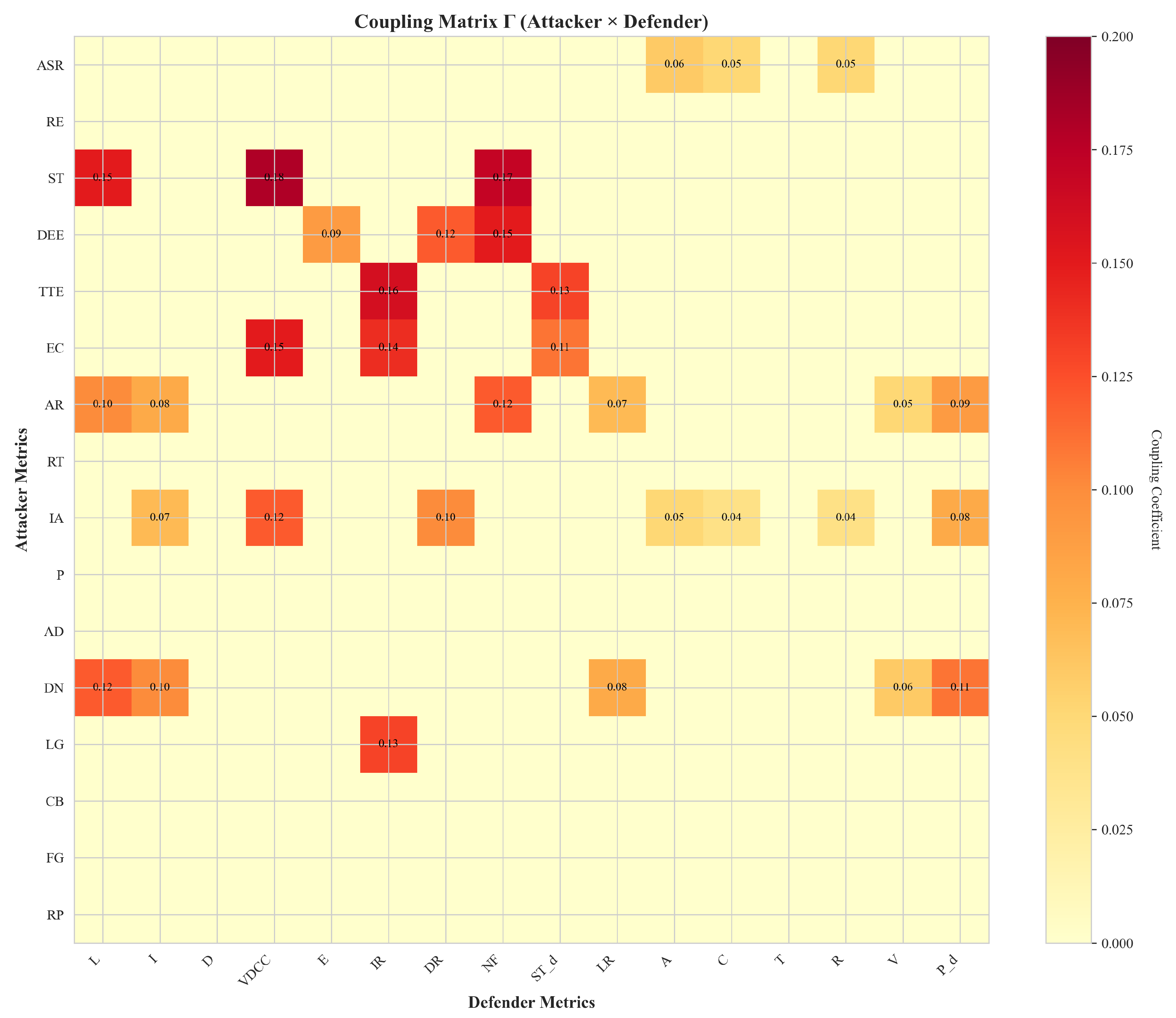
Figure A2.
Before/after distributions for selected attacker metrics across cases. Linked metrics (, DEE, AR) shift modestly downward; controls (RE, CB) remain stable. This demonstrates selective, realistic shifts where is nonzero, rather than global collapse. Zero cells (pale) in the coupling heatmap indicate no assumed linkage under . In the heatmap (Figure A1), defender metrics use subscript notation (, ) to distinguish from attacker metrics (, P).
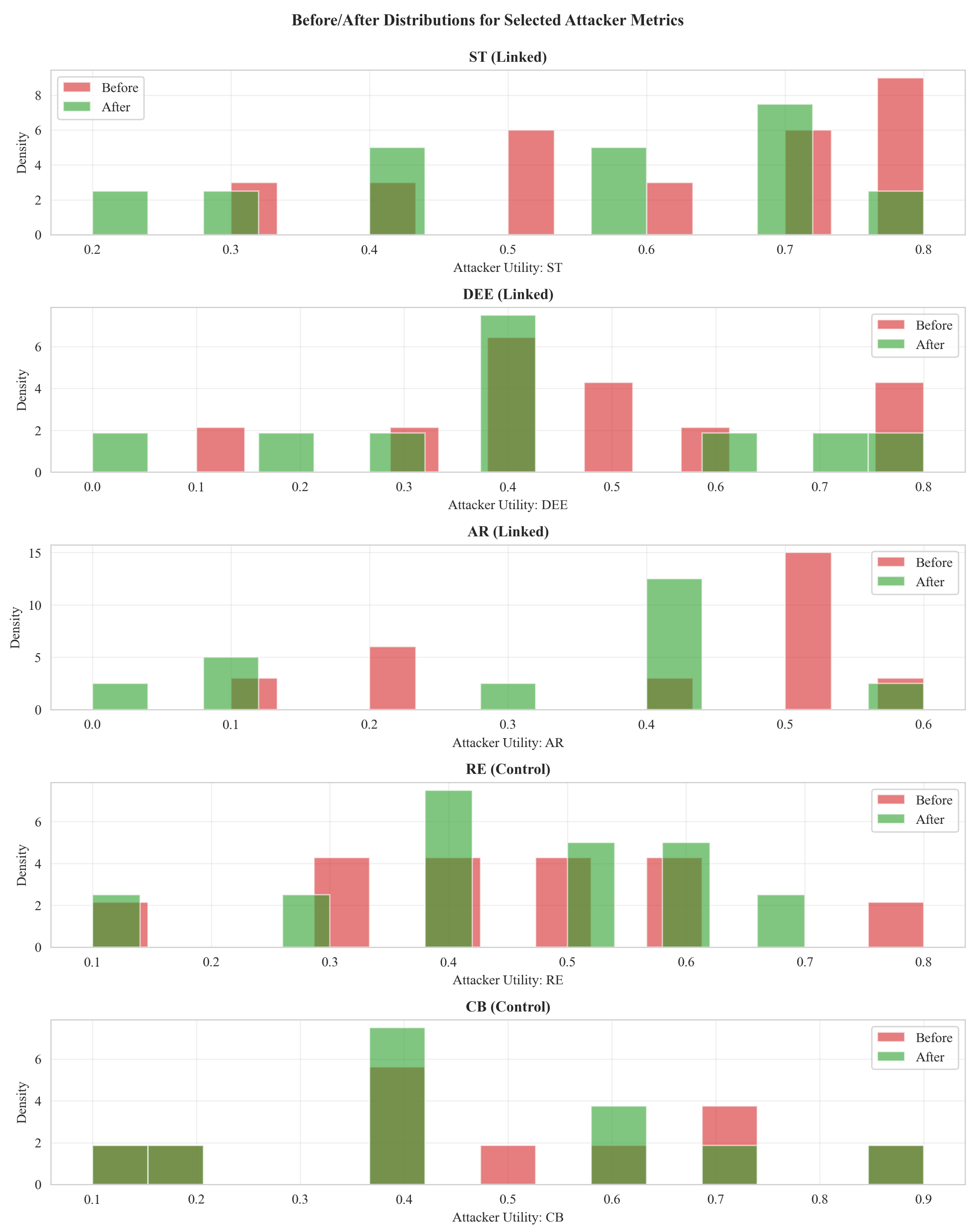
Figure A3.
Bipartite linkage graph: attacker metrics (left) and defender metrics (right). Edge widths proportional to . This visualizes the structural prior behind the calibration, making explicit which defender capabilities suppress which attacker utilities.
Figure A3.
Bipartite linkage graph: attacker metrics (left) and defender metrics (right). Edge widths proportional to . This visualizes the structural prior behind the calibration, making explicit which defender capabilities suppress which attacker utilities.
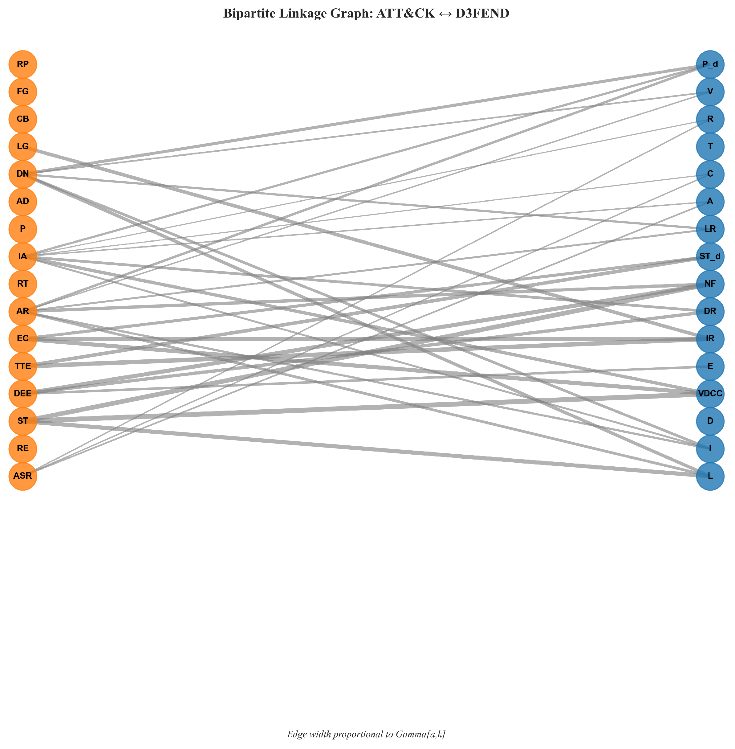
Figure A4.
Per-case waterfall: defender uplift (), attacker change (), and net Readiness. The dotted horizontal line at 0 marks the baseline. Net Readiness equals the difference between defender uplift (green) and attacker suppression (red). This clarifies how defender improvements and attacker suppression combine to yield net readiness gains. All cases show positive readiness improvement.
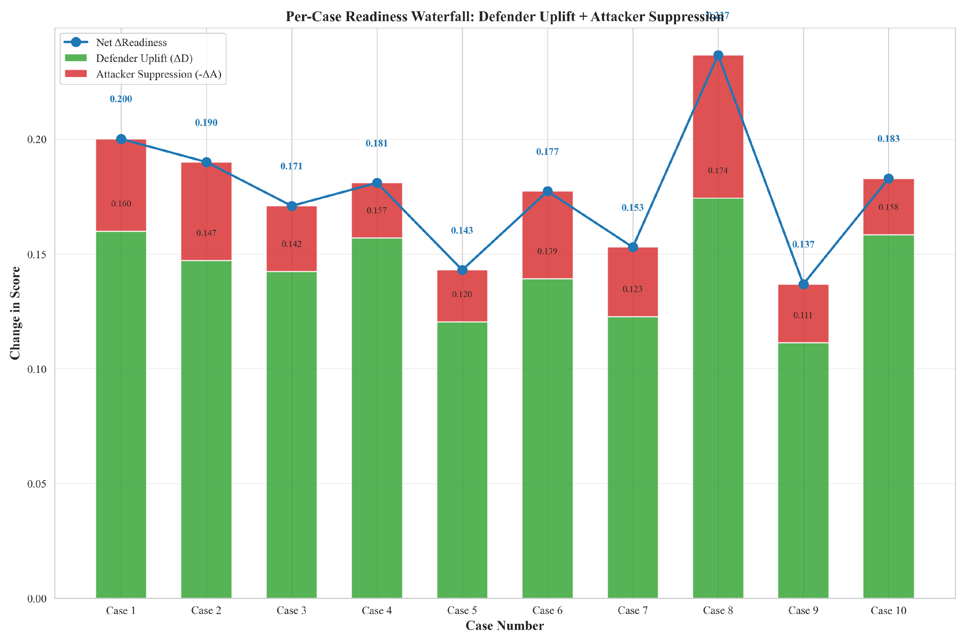
Appendix B.6. Optional Fuzzy Robustness (Not Used for Tables 4–5)
Scope.
This appendix provides a compact, reproducible fuzzy formulation (Mamdani min–max, centroid over ) that can be used to stress-test the readiness scoring, but it was not used to compute the main payoff matrices in Tables 4–5.
Specification
Inputs (normalized to ): EvidenceQuality, DetectionCoverage, ResponseLatency; Output: ForensicReadinessScore. Triangular membership functions and labels (Low/Medium/High for the first two, Fast/Moderate/Slow for latency) are given in Table S#, with the output Low/Medium/High in Table S#. The full rule table appears in Table S#, and Algorithm S# summarizes the pipeline. A perturbation on shows small variation (MAD ), indicating qualitative robustness of the readiness ranking.
Appendix B.7. Pure Nash Equilibrium Verification
A pure-strategy Nash equilibrium requires that is a best response to and is a best response to . We verify PNE by a full best-response scan: for each defender action (), we compute the (possibly set-valued) attacker best-response set ; for each attacker action (), we compute the defender set . A profile is a PNE iff and . Exhaustive enumeration over all pairs confirms that is the unique PNE.
Appendix B.8. Equilibrium Computation Details
Mixed Nash equilibria (MNE) were computed using the nashpy vertex_enumeration method [52] on the bimatrix game (non-zero-sum), where A and D are attacker and defender utility matrices constructed independently from ATT&CK→D3FEND mappings (Section 3.4.3).
Sign convention.
Both A and D are utilities to be maximized. We therefore pass Game(A, D) directly to the solver. When presenting defender costsC for interpretability, we convert to utilities via . In our implementation, D is already a utility matrix (higher is better), so no transformation is needed.
Main results (non-zero-sum).
For , vertex enumeration yields exactly one equilibrium, which is pure at . Support enumeration on returns the same single equilibrium.
Zero-sum variant.
For the zero-sum transform , vertex enumeration returns exactly five equilibria: two pure at and , and three mixed with supports , , and . Support enumeration reports only three equilibria on this instance; therefore, we treat vertex enumeration as the primary method and ground truth. All five equilibria satisfy first-order optimality (KKT) conditions—we numerically verified KKT feasibility, dual feasibility, and complementarity—and have tiny best-response residuals (on the order of for all equilibria, computed as the difference between maximum and minimum expected payoffs within support). These results are provided as a robustness check; policy conclusions in the main text are based on the non-zero-sum bimatrix .
All code—including exact payoff matrices—is archived in the repository (Section B). We provide two driver scripts for equilibrium computation: one for the non-zero-sum bimatrix and one for the zero-sum variant . Solver versioning and environment details are documented in the repository. No ad-hoc tie-breaking was required; all reported solutions are bona fide Nash equilibria.
Non-degeneracy and ε-perturbation.
The scaling from to with integer rounding could, in principle, introduce degeneracy (ties). Empirically, all reported equilibria are non-degenerate: (i) the unique PNE in has distinct payoffs at equilibrium; (ii) all equilibria in and have well-defined supports with equal payoffs only within support. We also performed -perturbation tests (uniform noise with ): the number and type of equilibria remained unchanged for and remained five for at , with coordinate differences effectively zero for . This indicates numerical stability to small perturbations.
Appendix B.9. Zero-sum Sensitivity Variant (A,-D)
For exploratory purposes, we analyze the zero-sum sensitivity variant . Unlike the main non-zero-sum bimatrix , G yields five equilibria under vertex enumeration: two pure-strategy equilibria (MNE 2: and MNE 4: ) and three mixed-strategy equilibria (MNE 1, MNE 3, MNE 5). These results are provided only as a robustness check; all policy conclusions are drawn from .
Figure A5 shows the equilibrium probability distributions for all five equilibria; Figure A6 contrasts the unique PNE from with the two pure equilibria from . Figure A7 provides a grid view of all five equilibria.
Figure A5.
All five equilibria in the zero-sum variant : 2 pure + 3 mixed. Bars show equilibrium probabilities over strategies. MNE 2 and MNE 4 are pure-strategy equilibria; MNE 1, MNE 3, and MNE 5 are mixed-strategy equilibria. Note: Main results use the non-zero-sum bimatrix , which yields a single equilibrium at .
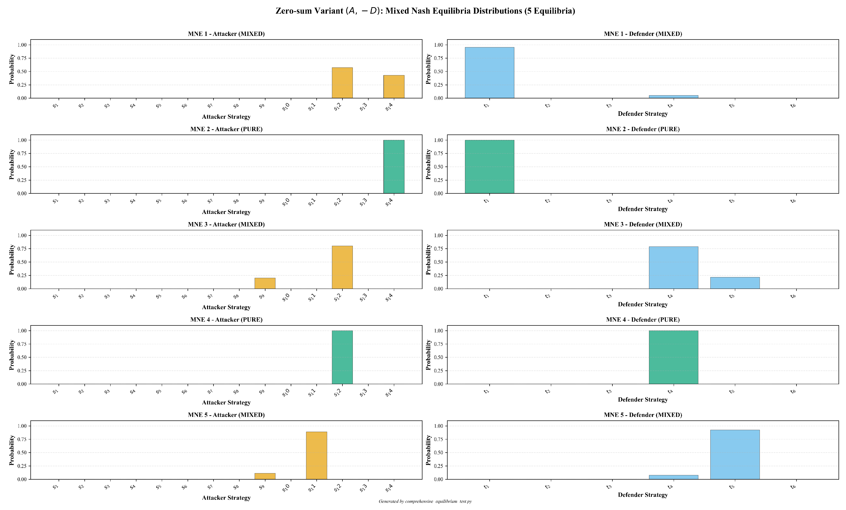
Table A2.
Zero-sum sensitivity variant : Complete support sets and probability distributions for all five Mixed Nash Equilibria (MNE). Only strategies with non-zero probabilities are shown. Probabilities rounded to four decimal places. MNE 2 and MNE 4 are pure-strategy equilibria; MNE 1, MNE 3, and MNE 5 are mixed-strategy equilibria. Note: These equilibria are from the zero-sum transform ; main results use the non-zero-sum bimatrix .
| MNE | Attacker Strategy | Defender Strategy |
|---|---|---|
| MNE 1 | : Command and Control (0.5714) | : Model (0.9512) |
| (mixed) | : Impact (0.4286) | : Isolate (0.0488) |
| MNE 2 | : Impact (1.0000) | : Model (1.0000) |
| (pure) | ||
| MNE 3 | : Discovery (0.2000) | : Isolate (0.7857) |
| (mixed) | : Command and Control (0.8000) | : Deceive (0.2143) |
| MNE 4 | : Command and Control (1.0000) | : Isolate (1.0000) |
| (pure) | ||
| MNE 5 | : Discovery (0.1111) | : Isolate (0.0769) |
| (mixed) | : Collection (0.8889) | : Deceive (0.9231) |
Figure A6.
Left: unique PNE for at . Middle/Right: the two pure equilibria in : MNE 2 at and MNE 4 at . Note: Main results use the non-zero-sum bimatrix .
Figure A6.
Left: unique PNE for at . Middle/Right: the two pure equilibria in : MNE 2 at and MNE 4 at . Note: Main results use the non-zero-sum bimatrix .
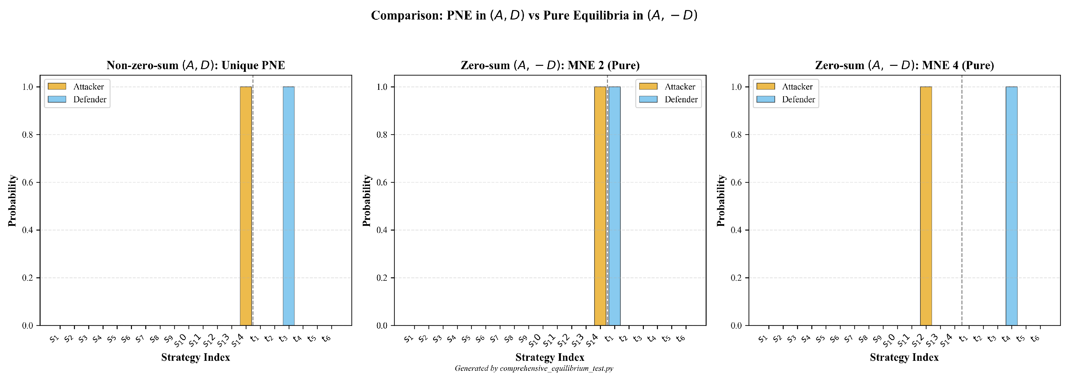
Figure A7.
Grid view of attacker/defender equilibrium distributions for each of the five equilibria in the zero-sum variant . MNE 2 and MNE 4 are pure-strategy equilibria; MNE 1, MNE 3, and MNE 5 are mixed-strategy equilibria. See Table A2 for exact probabilities and support sets. Note: Main results use the non-zero-sum bimatrix , which yields a single equilibrium at .
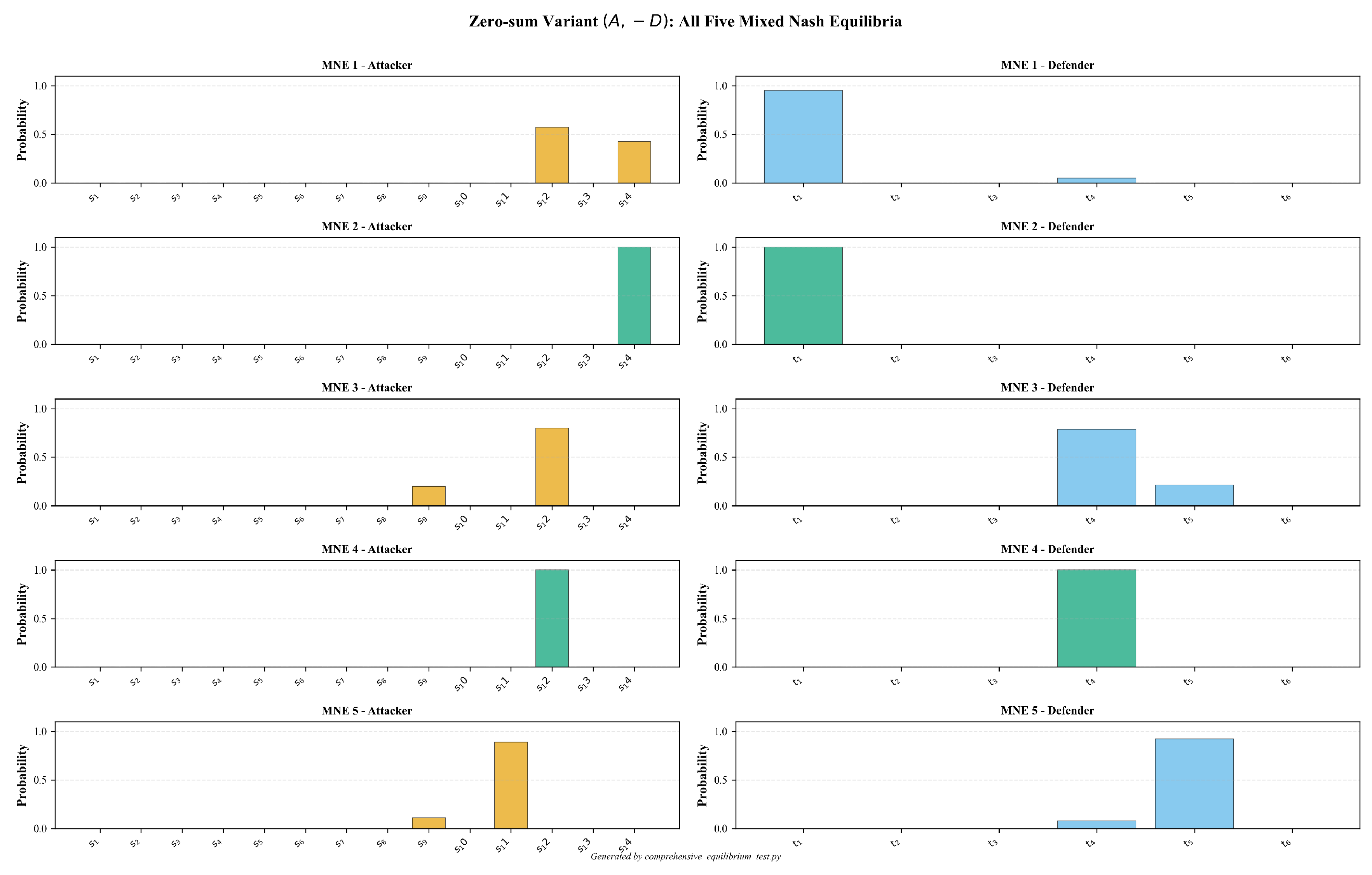
Table A3.
Six-decimal AHP-derived metric weights (attacker/defender).
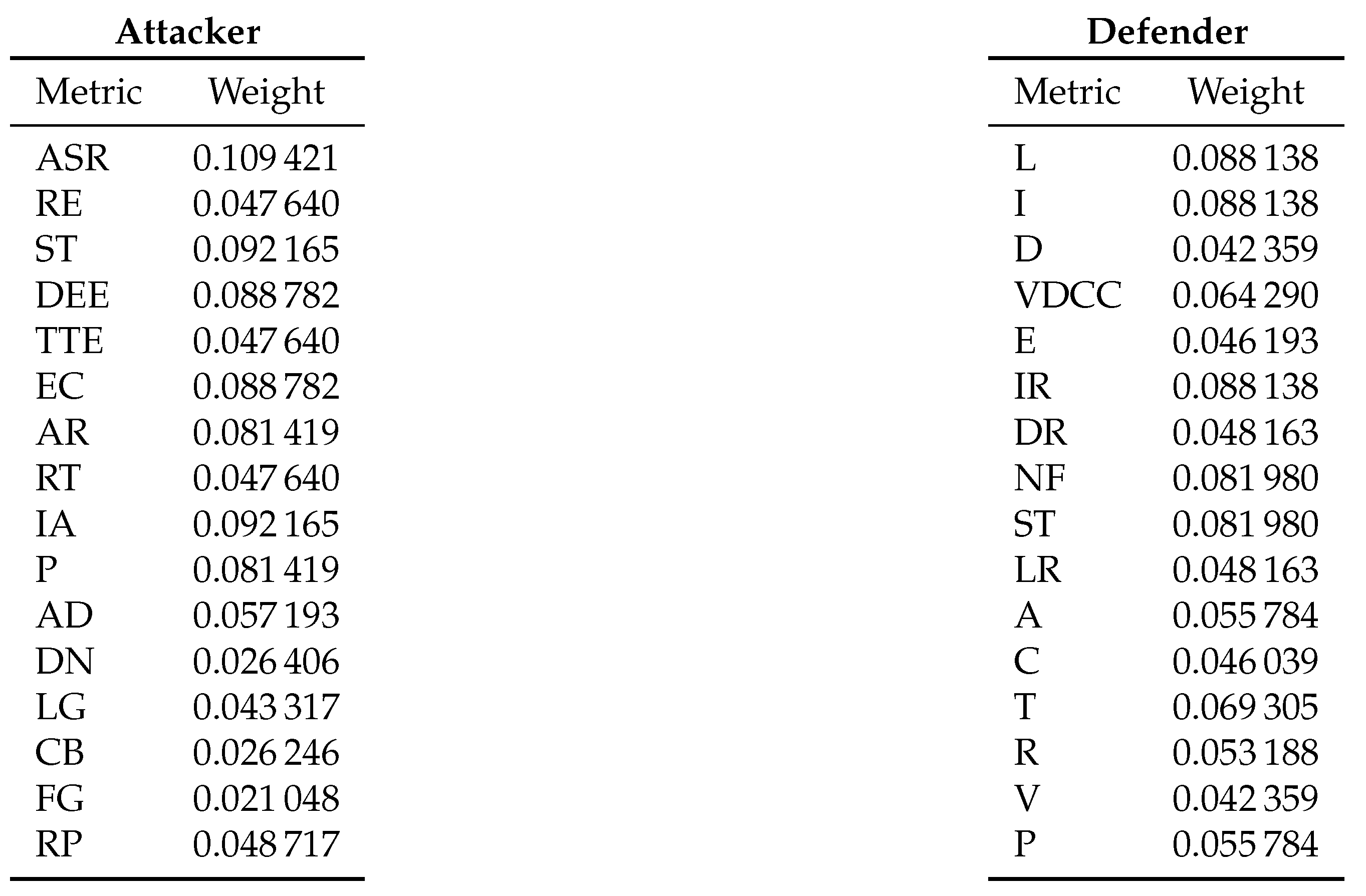
Table A4.
Consistency diagnostics for aggregated AHP matrices.
| Matrix | n | λmax | CI | CR | GCI | Koczkodaj |
| Attacker | 16 | 16.452 800 | 0.030 200 | 0.019 000 | 0.066 600 | 0.875 000 |
| Defender | 16 | 16.315 700 | 0.021 000 | 0.013 200 | 0.047 700 | 0.500 000 |
Figure A8.
AHP rank stability under local perturbations. For each metric i, all pairwise comparisons in row/column i are shifted by one 1–9 Saaty step and multiplicative noise is applied; reciprocity is restored and priorities are recomputed. Bars show mean absolute rank change (lower = more stable). Left: attacker; right: defender.
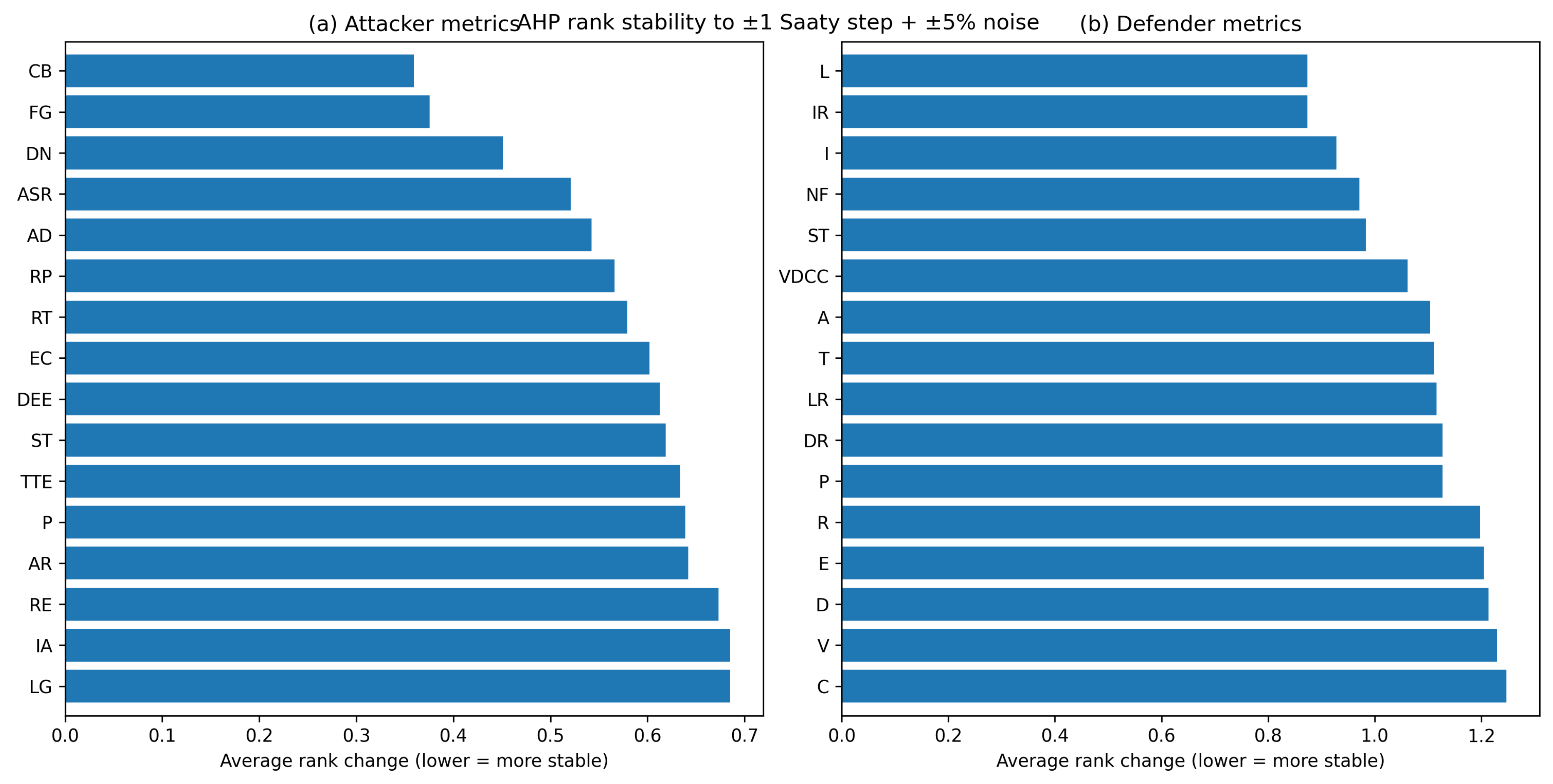
Figure A9.
Per-expert Consistency Ratio (CR) and Demographics. Violin plots for attacker and defender experts showing CR distributions. Dashed line indicates . Anonymized demographics (years of experience, primary domain expertise, geographic region) and per-expert CR values are provided in the Supplementary Materials (Section B).
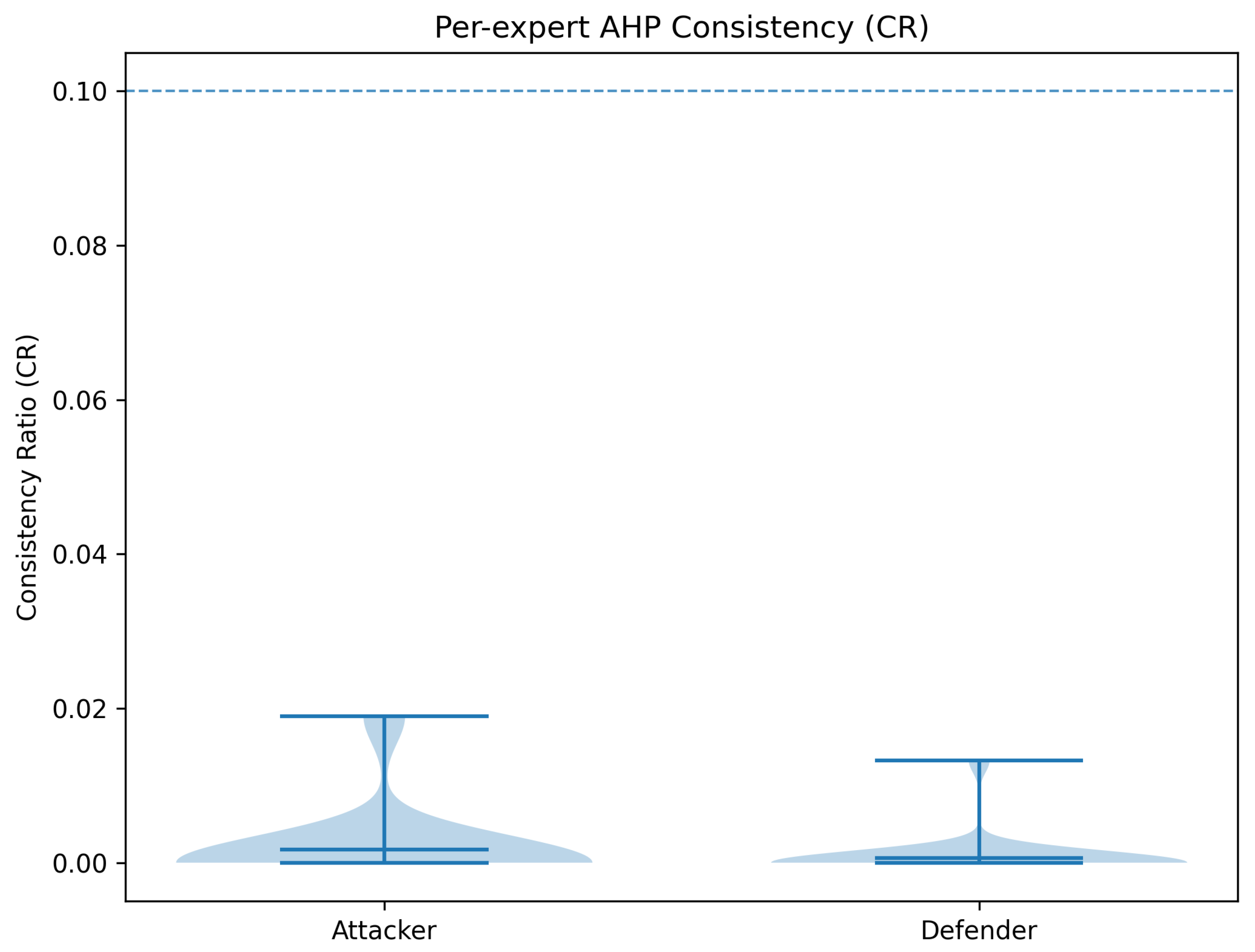
Table A5.
ATT&CK tactic × D3FEND control-family coverage counts (family-coverage). Each cell shows : the number of unique instances with at least one mapped D3FEND technique in family f, de-duplicated once per (see Eq. 4.2.0.1 and Section 4.2). Versions: ATT&CK Enterprise v13.1; D3FEND v0.12.0-BETA-2 (snapshot Mar–May 2023). Raw data extracted from STIX 2.1 JSON files and mapping CSVs (see Section B).
| ATT&CK Tactic | Model | Harden | Detect | Isolate | Deceive | Evict |
|---|---|---|---|---|---|---|
| Collection | 31 | 21 | 28 | 15 | 18 | 18 |
| Command and Control | 41 | 15 | 41 | 15 | 15 | 41 |
| Credential Access | 58 | 52 | 58 | 43 | 49 | 49 |
| Defense Evasion | 47 | 42 | 45 | 33 | 33 | 40 |
| Discovery | 27 | 18 | 24 | 13 | 15 | 18 |
| Execution | 30 | 22 | 27 | 18 | 19 | 21 |
| Exfiltration | 23 | 15 | 20 | 12 | 13 | 16 |
| Initial Access | 35 | 26 | 32 | 21 | 23 | 26 |
| Lateral Movement | 36 | 28 | 33 | 22 | 24 | 27 |
| Persistence | 38 | 29 | 35 | 24 | 26 | 28 |
| Privilege Escalation | 39 | 30 | 36 | 25 | 27 | 29 |
| Reconnaissance | 0 | 0 | 0 | 0 | 0 | 0 |
| Resource Development | 0 | 0 | 0 | 0 | 0 | 0 |
| Impact | 29 | 22 | 26 | 18 | 19 | 21 |
| Total | 371 | 274 | 360 | 253 | 228 | 288 |
Table A6.
ATT&CK tactic frequency counts across APT groups (de-duplicated). Each tactic is credited at most once per APT (preferring the most specific sub-technique evidence; see Eq. 4.2.0.2 and Section 4.2). Raw counts shown; shares and per-APT normalizations are available in the repository CSV exports. Versions: ATT&CK Enterprise v13.1; D3FEND v0.12.0-BETA-2 (snapshot Mar–May 2023).
| ATT&CK Tactic | Frequency |
|---|---|
| Collection | 8 |
| Command and Control | 9 |
| Credential Access | 10 |
| Defense Evasion | 10 |
| Discovery | 8 |
| Execution | 9 |
| Exfiltration | 7 |
| Initial Access | 9 |
| Lateral Movement | 9 |
| Persistence | 9 |
| Privilege Escalation | 9 |
| Reconnaissance | 0 |
| Resource Development | 0 |
| Impact | 8 |
| Total | 104 |
Table A7.
D3FEND defensive control family frequency counts across mapped APT–technique instances. Counts represent the number of unique APT–technique pairs mapped to each D3FEND family, aggregated across all ATT&CK tactics (see Section 4.2). Versions: ATT&CK Enterprise v13.1; D3FEND v0.12.0-BETA-2 (snapshot Mar–May 2023).
| D3FEND Control Family | Frequency |
|---|---|
| Model | 371 |
| Harden | 274 |
| Detect | 360 |
| Isolate | 253 |
| Deceive | 228 |
| Evict | 288 |
| Total | 1,774 |
Appendix B.10. Attacker Utility Metrics and Scoring Preferences (Full Details)
The complete detailed table for Attacker Utility Metrics and Scoring Preferences, originally referenced as Table 7 in the main text, is provided below. This table includes qualitative descriptions for each metric level (0, 0.1–0.3, 0.4–0.6, 0.7–0.9, 1) to guide metric evaluation. Each metric is evaluated on a continuous scale from 0 (least favorable) to 1 (most favorable).
Table A8.
Attacker Utility Metrics and Scoring Preferences (Full Details)
| Metric | Description | Score |
|---|---|---|
| Attack Success Rate (ASR) | Attack success rate is nearly nonexistent | 0 |
| Attacks are occasionally successful | 0.1–0.3 | |
| Attacks are successful about half of the time | 0.4–0.6 | |
| Attacks are usually successful | 0.7–0.9 | |
| Attacks are always successful | 1 | |
| Resource Efficiency (RE) | Attacks require considerable resources with low payoff | 0 |
| Attacks require significant resources but have a moderate payoff | 0.1–0.3 | |
| Attacks are somewhat resource efficient | 0.4–0.6 | |
| Attacks are quite resource efficient | 0.7–0.9 | |
| Attacks are exceptionally resource efficient | 1 | |
| Stealthiness (ST) | Attacks are always detected and attributed | 0 |
| Attacks are usually detected and often attributed | 0.1–0.3 | |
| Attacks are sometimes detected and occasionally attributed | 0.4–0.6 | |
| Attacks are seldom detected and rarely attributed | 0.7–0.9 | |
| Attacks are never detected nor attributed | 1 | |
| Data Exfiltration Effectiveness (DEE) | Data exfiltration attempts always fail | 0 |
| Data exfiltration attempts succeed only occasionally | 0.1–0.3 | |
| Data exfiltration attempts often succeed | 0.4–0.6 | |
| Data exfiltration attempts usually succeed | 0.7–0.9 | |
| Data exfiltration attempts always succeed | 1 | |
| Time-to-Exploit (TTE) | Vulnerabilities are never successfully exploited before patching | 0 |
| Vulnerabilities are exploited before patching only occasionally | 0.1–0.3 | |
| Vulnerabilities are often exploited before patching | 0.4–0.6 | |
| Vulnerabilities are usually exploited before patching | 0.7–0.9 | |
| Vulnerabilities are always exploited before patching | 1 | |
| Evasion of Countermeasures (EC) | Countermeasures always successfully thwart attacks | 0 |
| Countermeasures often successfully thwart attacks | 0.1–0.3 | |
| Countermeasures sometimes fail to thwart attacks | 0.4–0.6 | |
| Countermeasures often fail to thwart attacks | 0.7–0.9 | |
| Countermeasures never successfully thwart attacks | 1 | |
| Attribution Resistance (AR) | The attacker is always accurately identified | 0 |
| The attacker is often accurately identified | 0.1–0.3 | |
| The attacker is sometimes accurately identified | 0.4–0.6 | |
| The attacker is seldom accurately identified | 0.7–0.9 | |
| The attacker is never accurately identified | 1 | |
| Reusability of Attack Techniques (RT) | Attack techniques are always one-off, never reusable | 0 |
| Attack techniques are occasionally reusable | 0.1–0.3 | |
| Attack techniques are often reusable | 0.4–0.6 | |
| Attack techniques are usually reusable | 0.7–0.9 | |
| Attack techniques are always reusable | 1 | |
| Impact of Attacks (IA) | Attacks cause no notable disruption or loss | 0 |
| Attacks cause minor disruption or loss | 0.1–0.3 | |
| Attacks cause moderate disruption or loss | 0.4–0.6 | |
| Attacks cause major disruption or loss | 0.7–0.9 | |
| Attacks cause catastrophic disruption or loss | 1 | |
| Persistence (P) | The attacker cannot maintain control over compromised systems | 0 |
| The attacker occasionally maintains control over compromised systems | 0.1–0.3 | |
| The attacker often maintains control over compromised systems | 0.4–0.6 | |
| The attacker usually maintains control over compromised systems | 0.7–0.9 | |
| The attacker always maintains control over compromised systems | 1 | |
| Adaptability (AD) | The attacker is unable to adjust strategies in response to changing defenses | 0 |
| The attacker occasionally adjusts strategies in response to changing defenses | 0.1–0.3 | |
| The attacker often adjusts strategies in response to changing defenses | 0.4–0.6 | |
| The attacker usually adjusts strategies in response to changing defenses | 0.7–0.9 | |
| The attacker always adjusts strategies in response to changing defenses | 1 | |
| Deniability (DN) | The attacker cannot deny involvement in attacks | 0 |
| The attacker can occasionally deny involvement in attacks | 0.1–0.3 | |
| The attacker can often deny involvement in attacks | 0.4–0.6 | |
| The attacker can usually deny involvement in attacks | 0.7–0.9 | |
| The attacker can always deny involvement in attacks | 1 | |
| Longevity (LG) | The attacker’s operations are quickly disrupted | 0 |
| The attacker’s operations are often disrupted | 0.1–0.3 | |
| The attacker’s operations are occasionally disrupted | 0.4–0.6 | |
| The attacker’s operations are rarely disrupted | 0.7–0.9 | |
| The attacker’s operations are never disrupted | 1 | |
| Collaboration (CB) | The attacker never collaborates with others | 0 |
| The attacker occasionally collaborates with others | 0.1–0.3 | |
| The attacker often collaborates with others | 0.4–0.6 | |
| The attacker usually collaborates with others | 0.7–0.9 | |
| The attacker always collaborates with others | 1 | |
| Financial Gain (FG) | The attacker never profits from attacks | 0 |
| The attacker occasionally profits from attacks | 0.1–0.3 | |
| The attacker often profits from attacks | 0.4–0.6 | |
| The attacker usually profits from attacks | 0.7–0.9 | |
| The attacker always profits from attacks | 1 | |
| Reputation and Prestige (RP) | The attacker gains no reputation or prestige from attacks | 0 |
| The attacker gains little reputation or prestige from attacks | 0.1–0.3 | |
| The attacker gains some reputation or prestige from attacks | 0.4–0.6 | |
| The attacker gains considerable reputation or prestige from attacks | 0.7–0.9 | |
| The attacker’s reputation or prestige is greatly enhanced by each attack | 1 |
Appendix B.11. Defender Utility Metrics and Scoring Preferences (Full Details)
The complete detailed table for Defender Utility Metrics and Scoring Preferences, originally referenced as Table 8 in the main text, is provided below. This table includes qualitative descriptions for each metric level (0, 0.1–0.3, 0.4–0.6, 0.7–0.9, 1) to guide metric evaluation. Each metric is evaluated on a continuous scale from 0 (least favorable) to 1 (most favorable).
Table A9.
Defender Utility Metrics and Scoring Preferences (Full Details)
| Metric | Description | Score |
|---|---|---|
| Logging and Audit Trail Capabilities (L) | No logging or audit trail capabilities | 0 |
| Minimal or ineffective logging and audit trail capabilities | 0.1–0.3 | |
| Moderate logging and audit trail capabilities | 0.4–0.6 | |
| Robust logging and audit trail capabilities with some limitations | 0.7–0.9 | |
| Comprehensive and highly effective logging and audit trail capabilities | 1 | |
| Integrity and Preservation of Digital Evidence (I) | Complete loss of all digital evidence, including backups | 0 |
| Severe damage or compromised backups with limited recoverability | 0.1–0.3 | |
| Partial loss of digital evidence, with some recoverable data | 0.4–0.6 | |
| Reasonable integrity and preservation of digital evidence, with recoverable backups | 0.7–0.9 | |
| Full integrity and preservation of all digital evidence, including secure and accessible backups | 1 | |
| Documentation and Compliance with Digital Forensic Standards (D) | No documentation or non-compliance with digital forensic standards | 0 |
| Incomplete or inadequate documentation and limited adherence to digital forensic standards | 0.1–0.3 | |
| Basic documentation and partial compliance with digital forensic standards | 0.4–0.6 | |
| Well-documented processes and good adherence to digital forensic standards | 0.7–0.9 | |
| Comprehensive documentation and strict compliance with recognized digital forensic standards | 1 | |
| Volatile Data Capture Capabilities (VDCC) | No volatile data capture capabilities | 0 |
| Limited or unreliable volatile data capture capabilities | 0.1–0.3 | |
| Moderate volatile data capture capabilities | 0.4–0.6 | |
| Effective volatile data capture capabilities with some limitations | 0.7–0.9 | |
| Robust and reliable volatile data capture capabilities | 1 | |
| Encryption and Decryption Capabilities (E) | No encryption or decryption capabilities | 0 |
| Weak or limited encryption and decryption capabilities | 0.1–0.3 | |
| Moderate encryption and decryption capabilities | 0.4–0.6 | |
| Strong encryption and decryption capabilities with some limitations | 0.7–0.9 | |
| Highly secure encryption and decryption capabilities | 1 | |
| Incident Response Preparedness (IR) | No incident response plan or team in place | 0 |
| Initial incident response plan, not regularly tested or updated, with limited team capability | 0.1–0.3 | |
| Developed incident response plan, periodically tested, with trained team | 0.4–0.6 | |
| Comprehensive incident response plan, regularly tested and updated, with a well-coordinated team | 0.7–0.9 | |
| Advanced incident response plan, continuously tested and optimized, with a dedicated, experienced team | 1 | |
| Data Recovery Capabilities (DR) | No data recovery processes or tools in place | 0 |
| Basic data recovery tools, with limited effectiveness | 0.1–0.3 | |
| Advanced data recovery tools, with some limitations in terms of capabilities | 0.4–0.6 | |
| Sophisticated data recovery tools, with high success rates | 0.7–0.9 | |
| Comprehensive data recovery tools and processes, with excellent success rates | 1 | |
| Network Forensics Capabilities (NF) | No network forensic capabilities | 0 |
| Basic network forensic capabilities, limited to capturing packets or logs | 0.1–0.3 | |
| Developed network forensic capabilities, with ability to analyze traffic and detect anomalies | 0.4–0.6 | |
| Advanced network forensic capabilities, with proactive threat detection | 0.7–0.9 | |
| Comprehensive network forensic capabilities, with full spectrum threat detection and automated responses | 1 | |
| Staff Training and Expertise (STd) | No trained staff or expertise in digital forensics | 0 |
| Few staff members with basic training in digital forensics | 0.1–0.3 | |
| Several staff members with intermediate-level training, some with certifications | 0.4–0.6 | |
| Most staff members with advanced-level training, many with certifications | 0.7–0.9 | |
| All staff members are experts in digital forensics, with relevant certifications | 1 | |
| Legal & Regulatory Compliance (LR) | Non-compliance with applicable legal and regulatory requirements | 0 |
| Partial compliance with significant shortcomings | 0.1–0.3 | |
| Compliance with most requirements, some minor issues | 0.4–0.6 | |
| High compliance with only minor issues | 0.7–0.9 | |
| Full compliance with all relevant legal and regulatory requirements | 1 | |
| Accuracy (A) | No consistency in results, many errors and inaccuracies in digital forensic analysis | 0 |
| Frequent errors in analysis, high level of inaccuracy | 0.1–0.3 | |
| Some inaccuracies in results, needs further improvement | 0.4–0.6 | |
| High level of accuracy, few inconsistencies or errors | 0.7–0.9 | |
| Extremely accurate, consistent results with virtually no errors | 1 | |
| Completeness (C) | Significant data overlooked, very incomplete analysis | 0 |
| Some relevant data collected, but analysis remains substantially incomplete | 0.1–0.3 | |
| Most of the relevant data collected and analyzed, but some gaps remain | 0.4–0.6 | |
| High degree of completeness in data collection and analysis, minor gaps | 0.7–0.9 | |
| Comprehensive data collection and analysis, virtually no information overlooked | 1 | |
| Timeliness (T) | Extensive delays in digital forensic investigation process, no urgency | 0 |
| Frequent delays, slow response time | 0.1–0.3 | |
| Reasonable response time, occasional delays | 0.4–0.6 | |
| Quick response time, infrequent delays | 0.7–0.9 | |
| Immediate response, efficient process, no delays | 1 | |
| Reliability (R) | Unreliable techniques, inconsistent and unrepeatable results | 0 |
| Some reliability in techniques, but results are often inconsistent | 0.1–0.3 | |
| Mostly reliable techniques, occasional inconsistencies in results | 0.4–0.6 | |
| High reliability in techniques, few inconsistencies | 0.7–0.9 | |
| Highly reliable and consistent techniques, results are dependable and repeatable | 1 | |
| Validity (V) | No adherence to standards, methods not legally or scientifically acceptable | 0 |
| Minimal adherence to standards, many methods not acceptable | 0.1–0.3 | |
| Moderate adherence to standards, some methods not acceptable | 0.4–0.6 | |
| High adherence to standards, majority of methods are acceptable | 0.7–0.9 | |
| Strict adherence to standards, all methods used are legally and scientifically acceptable | 1 | |
| Preservation (Pd) | No procedures in place for evidence preservation, evidence frequently damaged or lost | 0 |
| Minimal preservation procedures, evidence sometimes damaged or lost | 0.1–0.3 | |
| Moderate preservation procedures, occasional evidence damage or loss | 0.4–0.6 | |
| Robust preservation procedures, rare instances of evidence damage or loss | 0.7–0.9 | |
| Comprehensive preservation procedures, virtually no damage or loss of evidence | 1 |
References
- Chen, P.; Desmet, L.; Huygens, C. A study on advanced persistent threats. In Proceedings of the Communications and Multimedia Security: 15th IFIP TC 6/TC 11 International Conference, CMS 2014, Aveiro, Portugal, 2014. Proceedings 15. Springer, 2014, September 25-26; pp. 63–72.
- Scott, J.S.R. Advanced Persistent Threats: Recognizing the Danger and Arming Your Organization. IT Professional 2015, 17. [Google Scholar]
- Rowlingson, R. A ten step process for forensic readiness. International Journal of Digital Evidence 2004, 2, 1–28. [Google Scholar]
- IBM. Cost of a Data Breach Report 2025: The AI Oversight Gap, 2025. Based on IBM analysis of research data independently compiled by Ponemon Institute.
- Bonderud, D. Cost of a data breach 2025: Financial industry, 2025.
- Johnson, R. 60 percent of small companies close within 6 months of being hacked,, 2019.
- Baker, P. The SolarWinds hack timeline: Who knew what, and when?, 2021.
- Batool, A.; Zowghi, D.; Bano, M. AI governance: a systematic literature review. AI and Ethics, 2025; 1–15. [Google Scholar]
- Wrightson, T. Advanced persistent threat hacking: the art and science of hacking any organization; McGraw-Hill Education Group, 2014.
- Årnes, A. Digital forensics; John Wiley & Sons, 2017.
- Griffith, S.B. Sun Tzu: The art of war; Vol. 39, Oxford University Press London, 1963.
- Myerson, R.B. Game theory; Harvard university press, 2013.
- Belton, V.; Stewart, T. Multiple criteria decision analysis: an integrated approach; Springer Science & Business Media, 2002.
- Lye, K.w.; Wing, J.M. Game strategies in network security. International Journal of Information Security 2005, 4, 71–86. [Google Scholar] [CrossRef]
- Roy, S.; Ellis, C.; Shiva, S.; Dasgupta, D.; Shandilya, V.; Wu, Q. A survey of game theory as applied to network security. In Proceedings of the 2010 43rd Hawaii International Conference on System Sciences. IEEE; 2010; pp. 1–10. [Google Scholar]
- Zhu, Q.; Basar, T. Game-theoretic methods for robustness, security, and resilience of cyberphysical control systems: games-in-games principle for optimal cross-layer resilient control systems. IEEE Control Systems Magazine 2015, 35, 46–65. [Google Scholar]
- Kent, K.; Chevalier, S.; Grance, T. Guide to integrating forensic techniques into incident. Tech. Rep. 800-86.
- Alpcan, T.; Başar, T. Network security: A decision and game-theoretic approach. Cambridge University Press 2010. [Google Scholar]
- Casey, E. Digital evidence and computer crime: Forensic science, computers, and the internet; Academic press, 2011.
- Manshaei, M.H.; Zhu, Q.; Alpcan, T.; Bacşar, T.; Hubaux, J.P. Game theory meets network security and privacy. Acm Computing Surveys (Csur) 2013, 45, 1–39. [Google Scholar] [CrossRef]
- Nisioti, A.; Loukas, G.; Rass, S.; Panaousis, E. Game-theoretic decision support for cyber forensic investigations. Sensors 2021, 21, 5300. [Google Scholar] [CrossRef] [PubMed]
- Hasanabadi, S.S.; Lashkari, A.H.; Ghorbani, A.A. A game-theoretic defensive approach for forensic investigators against rootkits. Forensic Science International: Digital Investigation 2020, 33, 200909. [Google Scholar] [CrossRef]
- Karabiyik, U.; Karabiyik, T. A game theoretic approach for digital forensic tool selection. Mathematics 2020, 8, 774. [Google Scholar] [CrossRef]
- Hasanabadi, S.S.; Lashkari, A.H.; Ghorbani, A.A. A memory-based game-theoretic defensive approach for digital forensic investigators. Forensic Science International: Digital Investigation 2021, 38, 301214. [Google Scholar] [CrossRef]
- Caporusso, N.; Chea, S.; Abukhaled, R. A game-theoretical model of ransomware. In Proceedings of the Advances in Human Factors in Cybersecurity: Proceedings of the AHFE 2018 International Conference on Human Factors in Cybersecurity, July 21-25, 2018, Loews Sapphire Falls Resort at Universal Studios, Orlando, Florida, USA 9. Springer, 2018, pp. 69–78.
- Kebande, V.R.; Venter, H.S. Novel digital forensic readiness technique in the cloud environment. Australian Journal of Forensic Sciences 2018, 50, 552–591. [Google Scholar] [CrossRef]
- Kebande, V.R.; Karie, N.M.; Choo, K.R.; Alawadi, S. Digital forensic readiness intelligence crime repository. Security and Privacy 2021, 4, e151. [Google Scholar] [CrossRef]
- Englbrecht, L.; Meier, S.; Pernul, G. Towards a capability maturity model for digital forensic readiness. Wireless Networks 2020, 26, 4895–4907. [Google Scholar] [CrossRef]
- Reddy, K.; Venter, H.S. The architecture of a digital forensic readiness management system. Computers & security 2013, 32, 73–89. [Google Scholar]
- Grobler, C.P.; Louwrens, C. Digital forensic readiness as a component of information security best practice. In Proceedings of the IFIP International Information Security Conference. Springer; 2007; pp. 13–24. [Google Scholar]
- Lakhdhar, Y.; Rekhis, S.; Sabir, E. A Game Theoretic Approach For Deploying Forensic Ready Systems. In Proceedings of the 2020 International Conference on Software, Telecommunications and Computer Networks (SoftCOM). IEEE; 2020; pp. 1–6. [Google Scholar]
- Elyas, M.; Ahmad, A.; Maynard, S.B.; Lonie, A. Digital forensic readiness: Expert perspectives on a theoretical framework. Computers & Security 2015, 52, 70–89. [Google Scholar] [CrossRef]
- Baiquni, I.Z.; Amiruddin, A. A case study of digital forensic readiness level measurement using DiFRI model. In Proceedings of the 2022 International Conference on Informatics, Multimedia, Cyber and Information System (ICIMCIS). IEEE. 2022; pp. 184–189. [Google Scholar]
- Rawindaran, N.; Jayal, A.; Prakash, E. Cybersecurity Framework: Addressing Resiliency in Welsh SMEs for Digital Transformation and Industry 5.0. Journal of Cybersecurity and Privacy 2025, 5, 17. [Google Scholar] [CrossRef]
- Trenwith, P.M.; Venter, H.S. Digital forensic readiness in the cloud. In Proceedings of the 2013 Information Security for South Africa. IEEE; 2013; pp. 1–5. [Google Scholar]
- Monteiro, D.; Yu, Y.; Zisman, A.; Nuseibeh, B. Adaptive Observability for Forensic-Ready Microservice Systems. IEEE Transactions on Services Computing 2023. [Google Scholar] [CrossRef]
- Xiong, W.; Legrand, E.; Åberg, O.; Lagerström, R. Cyber security threat modeling based on the MITRE Enterprise ATT&CK Matrix. Software and Systems Modeling 2022, 21, 157–177. [Google Scholar]
- Wang, J.; Neil, M. A Bayesian-network-based cybersecurity adversarial risk analysis framework with numerical examples. arXiv preprint, 2021; arXiv:2106.00471 2021. [Google Scholar]
- Usman, N.; Usman, S.; Khan, F.; Jan, M.A.; Sajid, A.; Alazab, M.; Watters, P. Intelligent dynamic malware detection using machine learning in IP reputation for forensics data analytics. Future Generation Computer Systems 2021, 118, 124–141. [Google Scholar] [CrossRef]
- Li, M.; Lal, C.; Conti, M.; Hu, D. LEChain: A blockchain-based lawful evidence management scheme for digital forensics. Future Generation Computer Systems 2021, 115, 406–420. [Google Scholar] [CrossRef]
- Soltani, S.; Seno, S.A.H. Detecting the software usage on a compromised system: A triage solution for digital forensics. Forensic Science International: Digital Investigation 2023, 44, 301484. [Google Scholar] [CrossRef]
- Rother, C.; Chen, B. Reversing File Access Control Using Disk Forensics on Low-Level Flash Memory. Journal of Cybersecurity and Privacy 2024, 4, 805–822. [Google Scholar] [CrossRef]
- Nikkel, B. Registration Data Access Protocol (RDAP) for digital forensic investigators. Digital Investigation 2017, 22, 133–141. [Google Scholar] [CrossRef]
- Nikkel, B. Fintech forensics: Criminal investigation and digital evidence in financial technologies. Forensic Science International: Digital Investigation 2020, 33, 200908. [Google Scholar] [CrossRef]
- Seo, S.; Seok, B.; Lee, C. Digital forensic investigation framework for the metaverse. The Journal of Supercomputing 2023, 79, 9467–9485. [Google Scholar] [CrossRef]
- Malhotra, S. Digital forensics meets ai: A game-changer for the 4th industrial revolution. In Artificial Intelligence and Blockchain in Digital Forensics; River Publishers, 2023; pp. 1–20.
- Tok, Y.C.; Chattopadhyay, S. Identifying threats, cybercrime and digital forensic opportunities in Smart City Infrastructure via threat modeling. Forensic Science International: Digital Investigation 2023, 45, 301540. [Google Scholar] [CrossRef]
- Han, K.; Choi, J.H.; Choi, Y.; Lee, G.M.; Whinston, A.B. Security defense against long-term and stealthy cyberattacks. Decision Support Systems 2023, 166, 113912. [Google Scholar] [CrossRef]
- Chandra, A.; Snowe, M.J. A taxonomy of cybercrime: Theory and design. International Journal of Accounting Information Systems 2020, 38, 100467. [Google Scholar] [CrossRef]
- Casey, E.; Barnum, S.; Griffith, R.; Snyder, J.; van Beek, H.; Nelson, A. Advancing coordinated cyber-investigations and tool interoperability using a community developed specification language. Digital investigation 2017, 22, 14–45. [Google Scholar] [CrossRef]
- Boyd, S.; Vandenberghe, L. Convex optimization; Cambridge university press, 2004.
- Knight, V.; Campbell, J. Nashpy: A Python library for the computation of Nash equilibria. Journal of Open Source Software 2018, 3, 904. [Google Scholar] [CrossRef]
- Zopounidis, C.; Pardalos, P.M. Handbook of multicriteria analysis; Vol. 103, Springer Science & Business Media, 2010.
- Bipm, I.; Ifcc, I.; Iso, I. IUPaP, and OImL. Evaluation of measurement data—Supplement 2008, 1. [Google Scholar]
- Saaty, T.L. Analytic hierarchy process. In Encyclopedia of operations research and management science; Springer, 2013; pp. 52–64.
- The MITRE Corporation. MITRE ATT&CK STIX Data, 2024. Structured Threat Information Expression (STIX 2.1) datasets for Enterprise, Mobile, and ICS ATT&CK.
Figure 2.
Zero-sum variant : convergence under discrete-time best-response dynamics from a grid of initial conditions (seed=42, step size=1, convergence tolerance=). The system converges to two pure attractors: and ; mixed equilibria are saddle/unstable under this dynamic. Note: Main results use the non-zero-sum bimatrix , which yields a single PNE at . See Section B.9 for details.
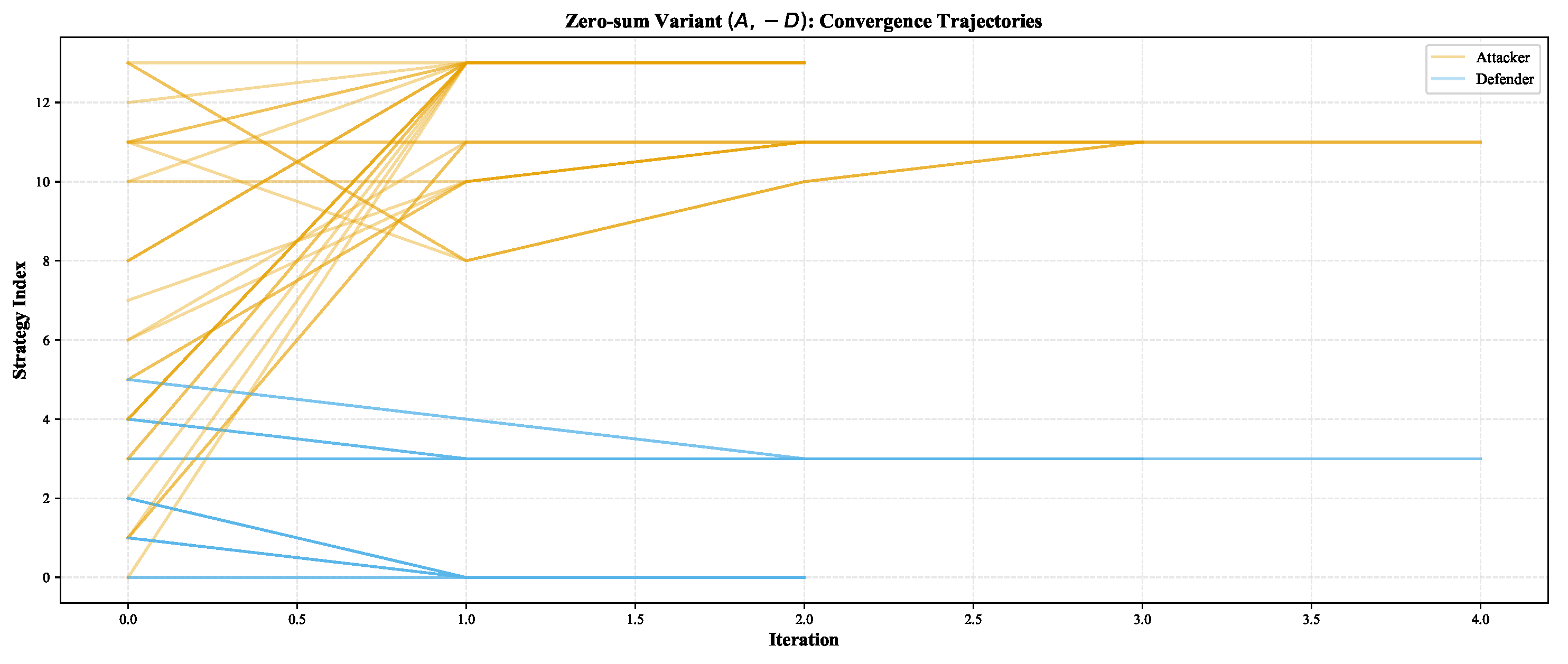
Figure 4.
Attacker and defender metric weights derived via AHP
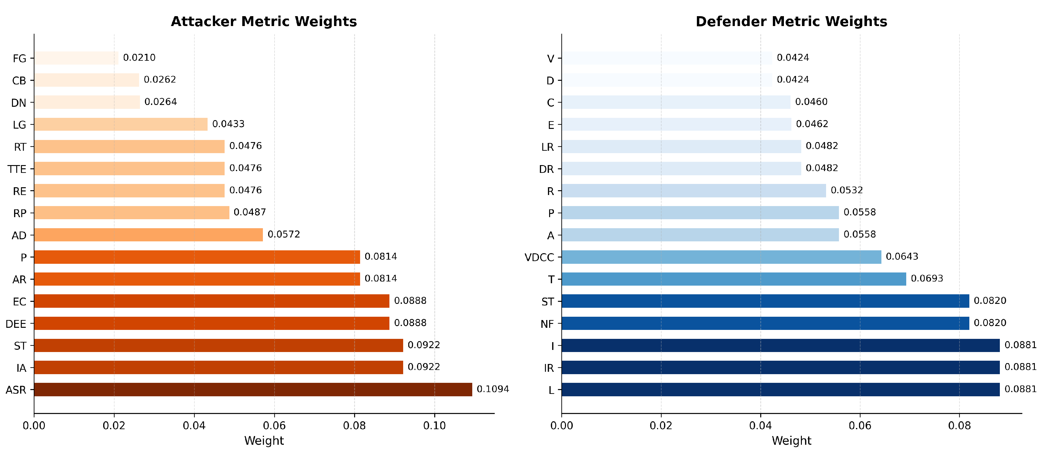
Figure 7.
Empirical frequency of D3FEND defensive control families (tactics) across mapped APT–technique instances derived from real-world data. Counts represent the number of unique APT–technique pairs mapped to each D3FEND family, aggregated across all ATT&CK tactics. Data extracted from MITRE STIX bundles for ten real APT groups (LeafMiner, Silent Librarian, OilRig, Ajax Security Team, Moses Staff, Cleaver, CopyKittens, APT33, APT39, MuddyWater). Y-axis: count; X-axis: D3FEND control family (Model, Harden, Detect, Isolate, Deceive, Evict). Versions: ATT&CK Enterprise v13.1; D3FEND v0.12.0-BETA-2 (snapshot Mar–May 2023). Raw data are provided in the Supplement (Table A7).

Figure 8.
Mean readiness score before and after implementation.
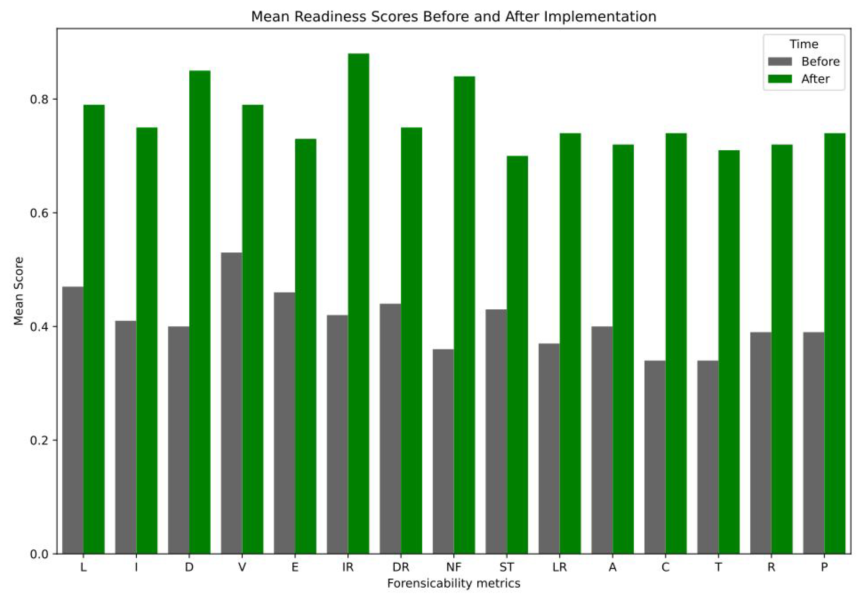
Figure 9.
AHP-based rank-stability under Saaty step plus noise (lower bars = more stable).
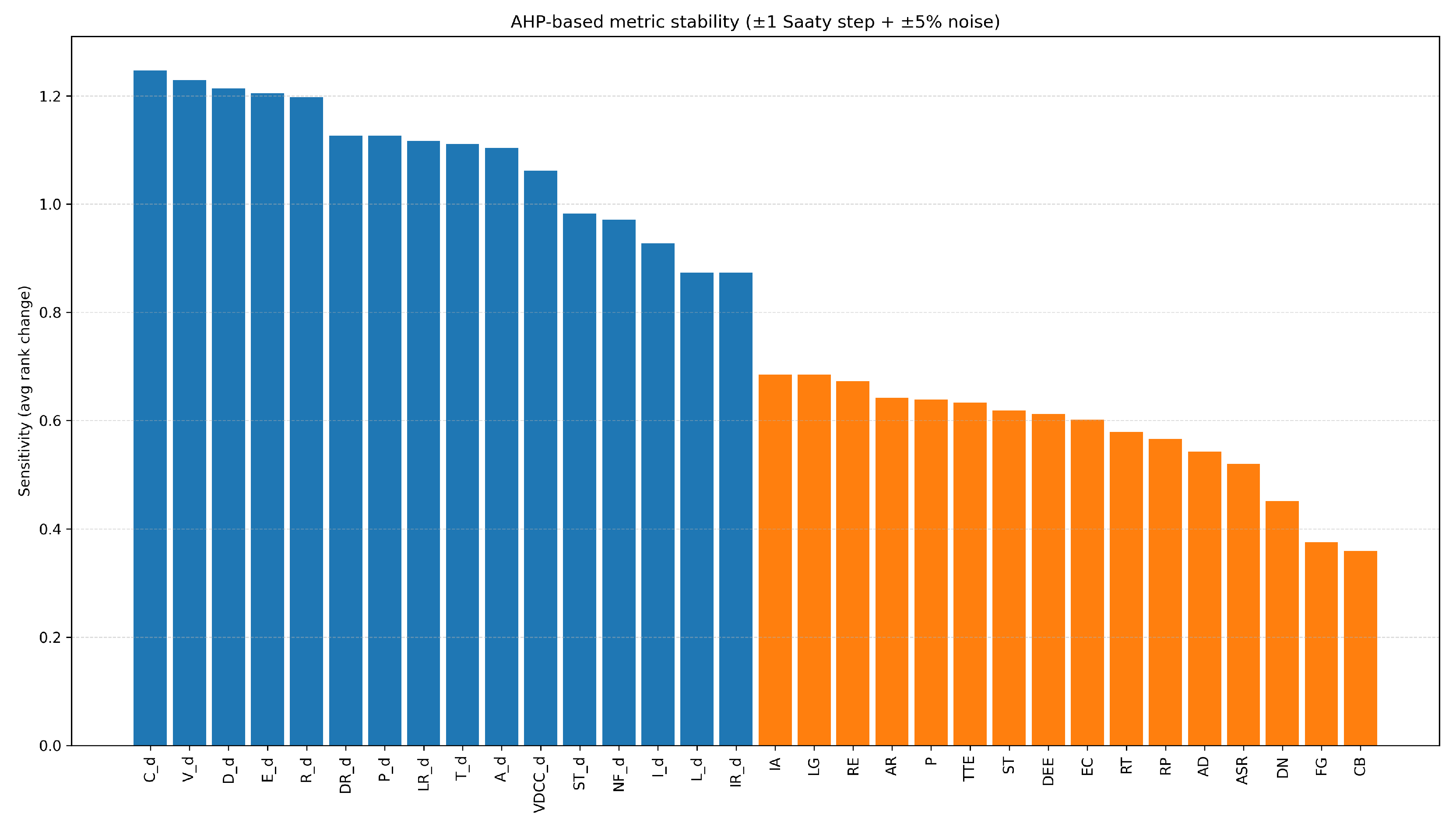
Figure 10.
Global sensitivity analysis of DFR metrics to readiness scores. Y-axis: absolute Pearson correlation coefficient (, unitless, range [0,1]); X-axis: metric ID (attacker: ASR, RE, ST, DEE, TTE, EC, AR, RT, IA, P, AD, DN, LG, CB, FG, RP; defender: L, I, D, VDCC, E, IR, DR, NF, STd, LR, A, C, T, R, V, Pd). Sensitivity computed from Monte Carlo draws sampling metric values independently from ; readiness computed via Eq. 10 using AHP-derived weights (Table 9). Higher bars indicate stronger influence on readiness variability.
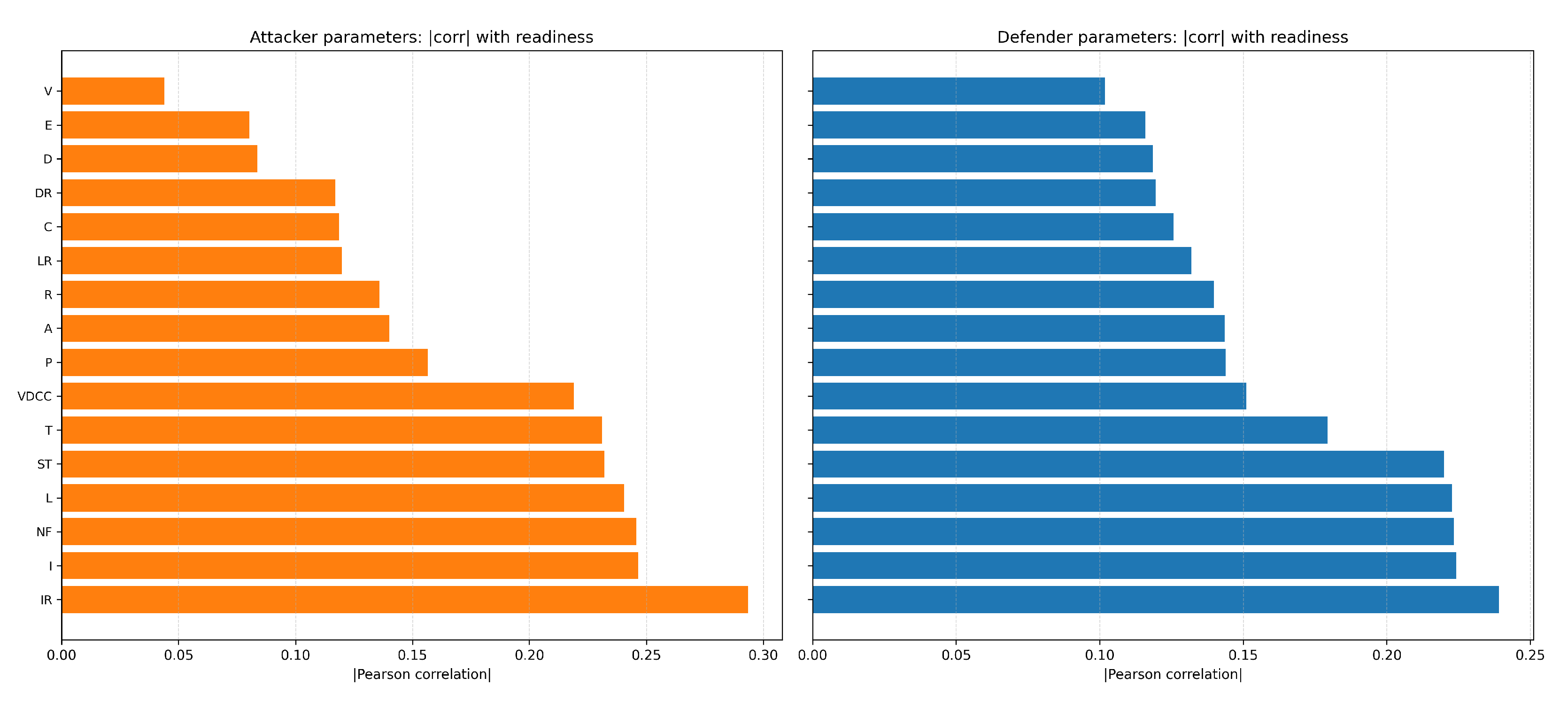
Figure 11.
Bivariate relationships between attacker metrics and readiness scores. Y-axis: readiness score (computed via Eq. 10, unitless, range approximately ); X-axis: attacker metric value (normalized ). Each panel shows one of the 16 attacker metrics (ASR, RE, ST, DEE, TTE, EC, AR, RT, IA, P, AD, DN, LG, CB, FG, RP); scatter points sampled from Monte Carlo draws with metric values independently sampled from and readiness computed using AHP-derived weights (Table 9).
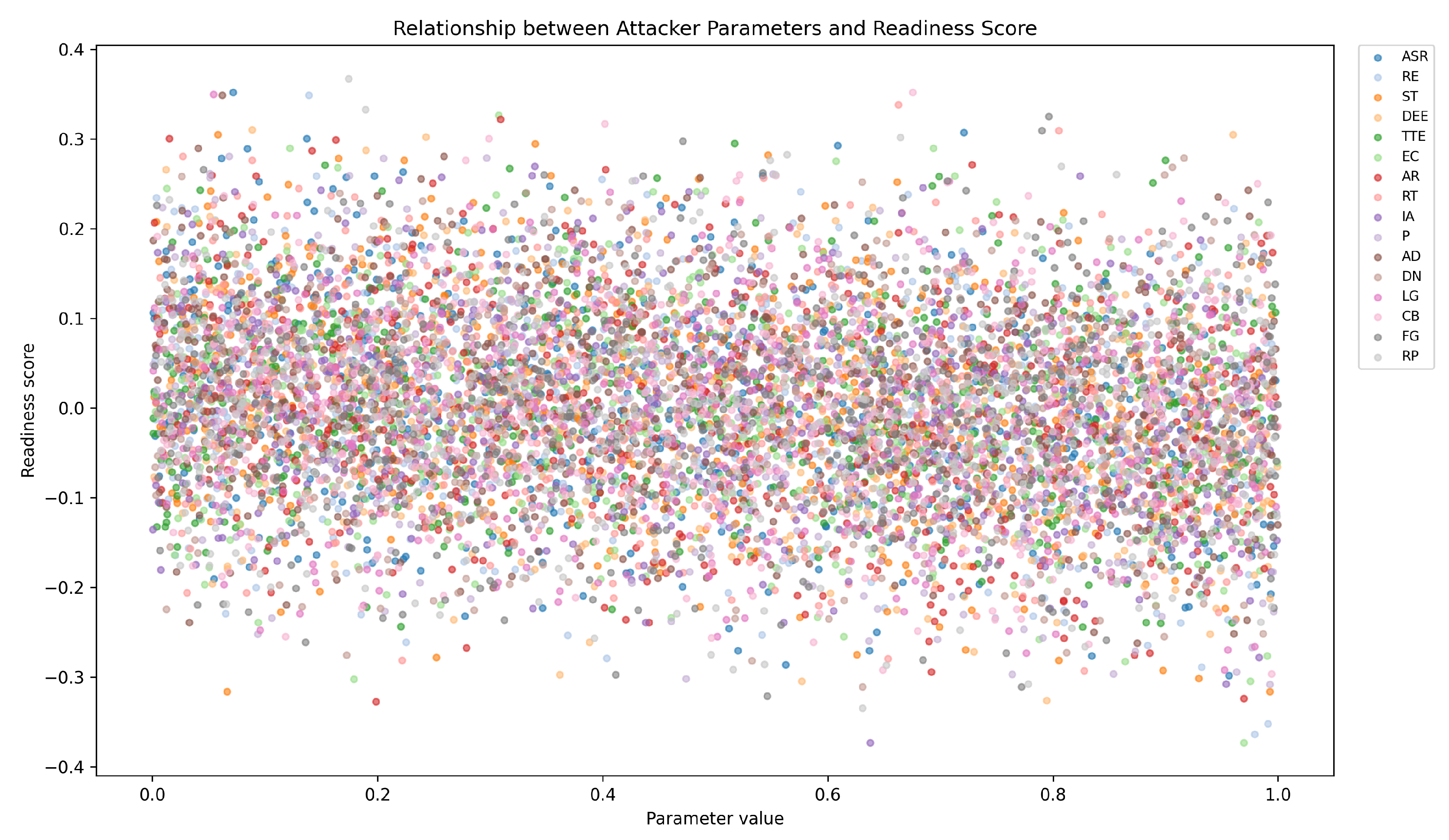
Figure 12.
Bivariate relationships between defender metrics and readiness scores. Y-axis: readiness score (computed via Eq. 10, unitless, range approximately ); X-axis: defender metric value (normalized ). Each panel shows one of the 16 defender metrics (L, I, D, VDCC, E, IR, DR, NF, STd, LR, A, C, T, R, V, Pd); scatter points sampled from Monte Carlo draws with metric values independently sampled from and readiness computed using AHP-derived weights (Table 9).
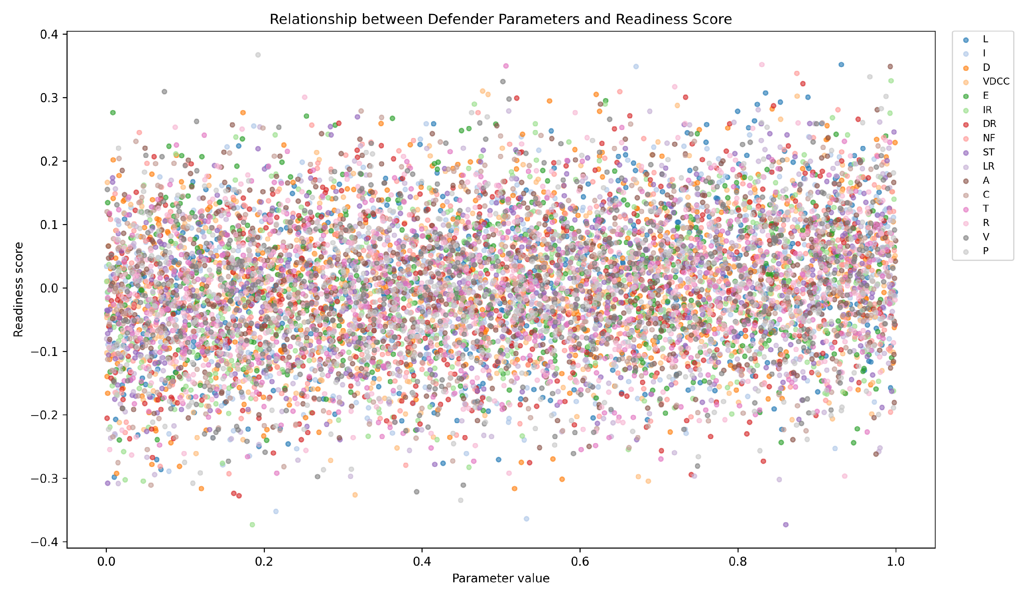
Figure 13.
Distribution of standardized (z-scored) readiness values across Monte Carlo simulation ( draws). Y-axis: frequency (count); X-axis: standardized readiness score (unitless, centered at zero). Readiness computed via Eq. 10 using AHP-derived weights (Table 9); raw readiness values approximately in (defender utility minus attacker utility). The near-symmetric distribution indicates balanced variability around the mean.
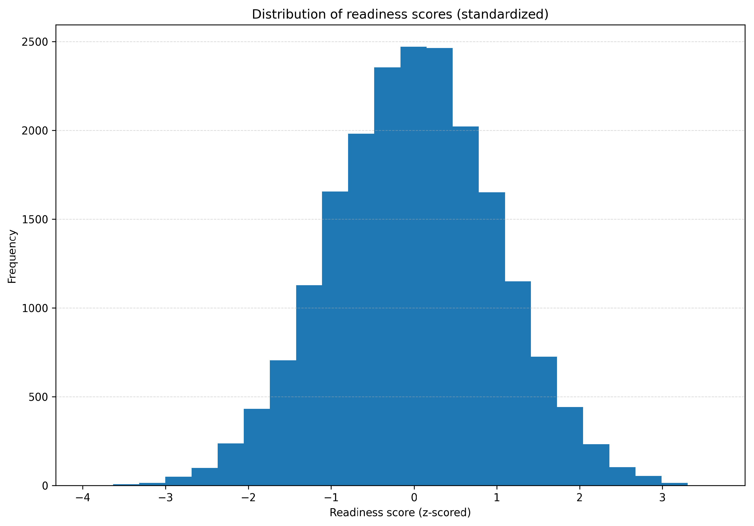
Figure 14.
Implementation roadmap and outcomes. Left: key adoption challenges. Center: phased workflow for deploying the game-theoretic DFR framework. Right: expected outcomes. Bottom band: cross-cutting enablers (policy, collaboration, upskilling, and measurement).
Figure 14.
Implementation roadmap and outcomes. Left: key adoption challenges. Center: phased workflow for deploying the game-theoretic DFR framework. Right: expected outcomes. Bottom band: cross-cutting enablers (policy, collaboration, upskilling, and measurement).
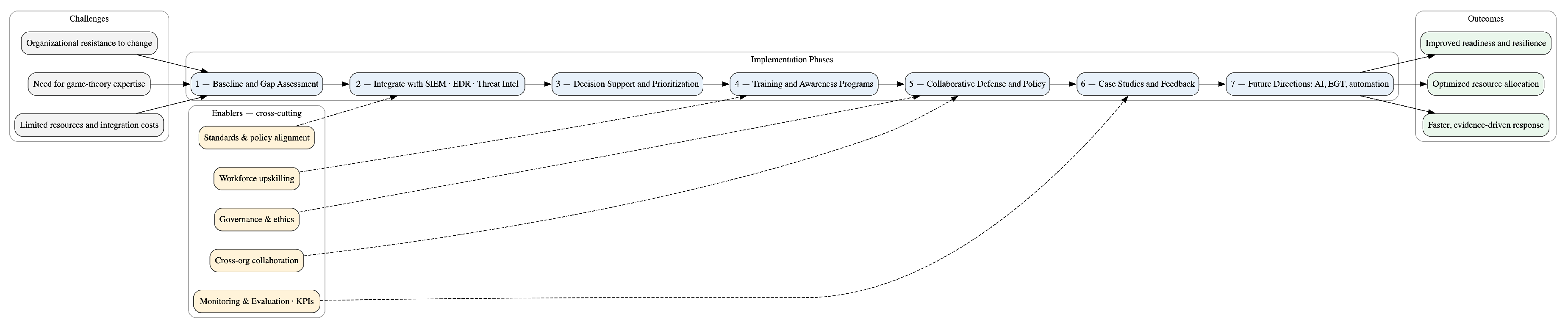
Figure 15.
Evolution of attacker and defender strategies in EGT simulation.

Figure 16.
Effect of attacks on investigation phases: (a) Pareto chart; (b) Attacker and defender utility; (c) Utility coordination visualization.
Figure 16.
Effect of attacks on investigation phases: (a) Pareto chart; (b) Attacker and defender utility; (c) Utility coordination visualization.
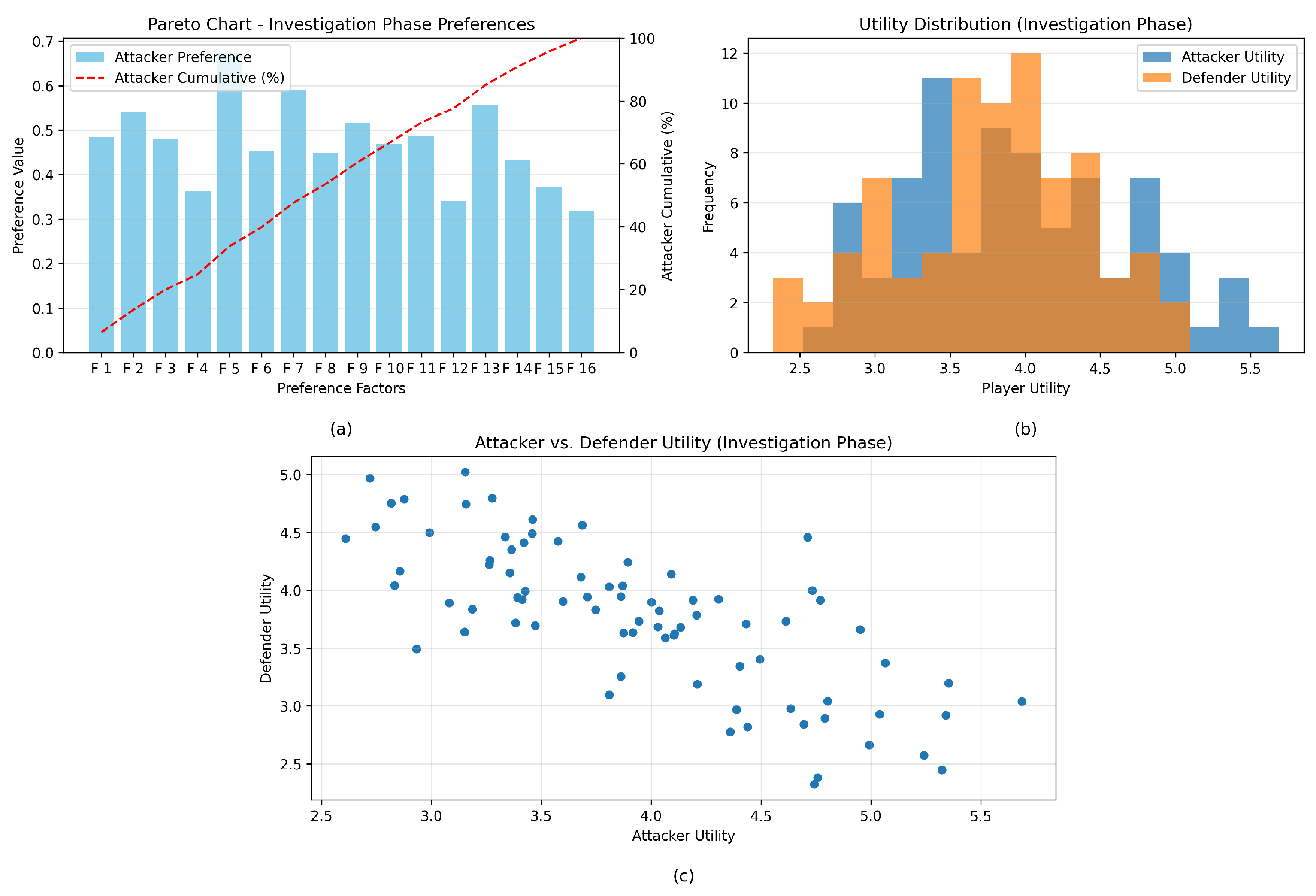
Figure 17.
Defender readiness vs. training level in three maturity regimes: (a) Junior+Mid+Senior, (b) Mid+Senior, and (c) Senior.
Figure 17.
Defender readiness vs. training level in three maturity regimes: (a) Junior+Mid+Senior, (b) Mid+Senior, and (c) Senior.
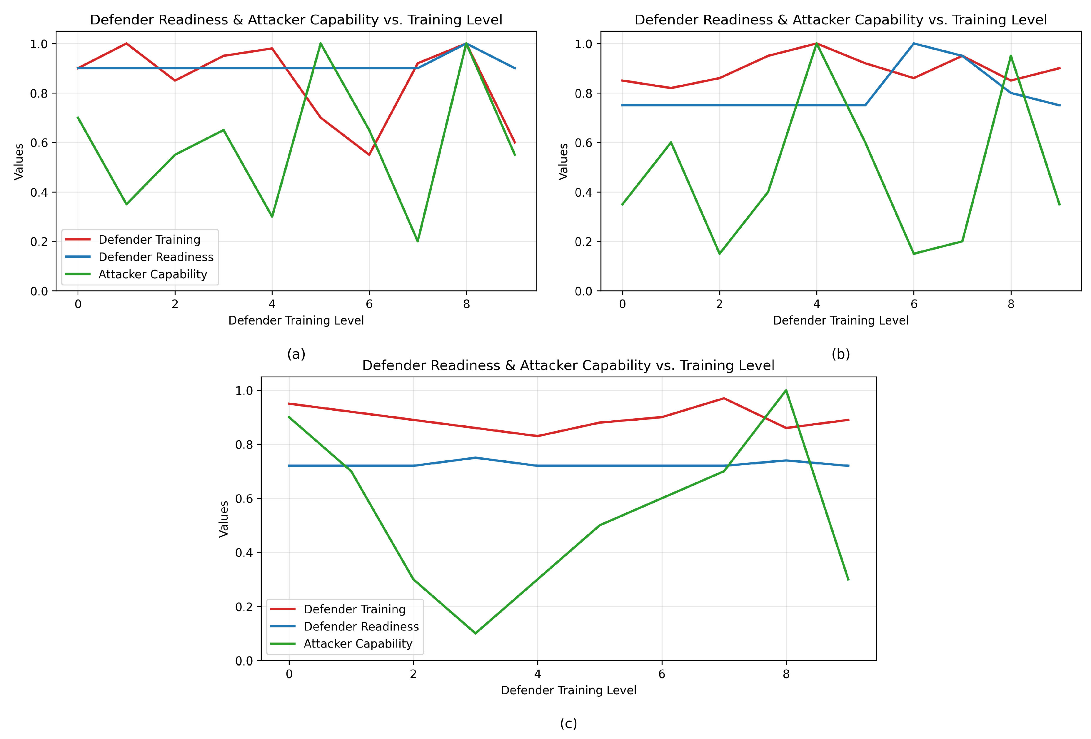
Figure 18.
Impact comparison for SMEs and SMBs under SQLi and DDoS scenarios (baseline vs. irrational).
Figure 18.
Impact comparison for SMEs and SMBs under SQLi and DDoS scenarios (baseline vs. irrational).
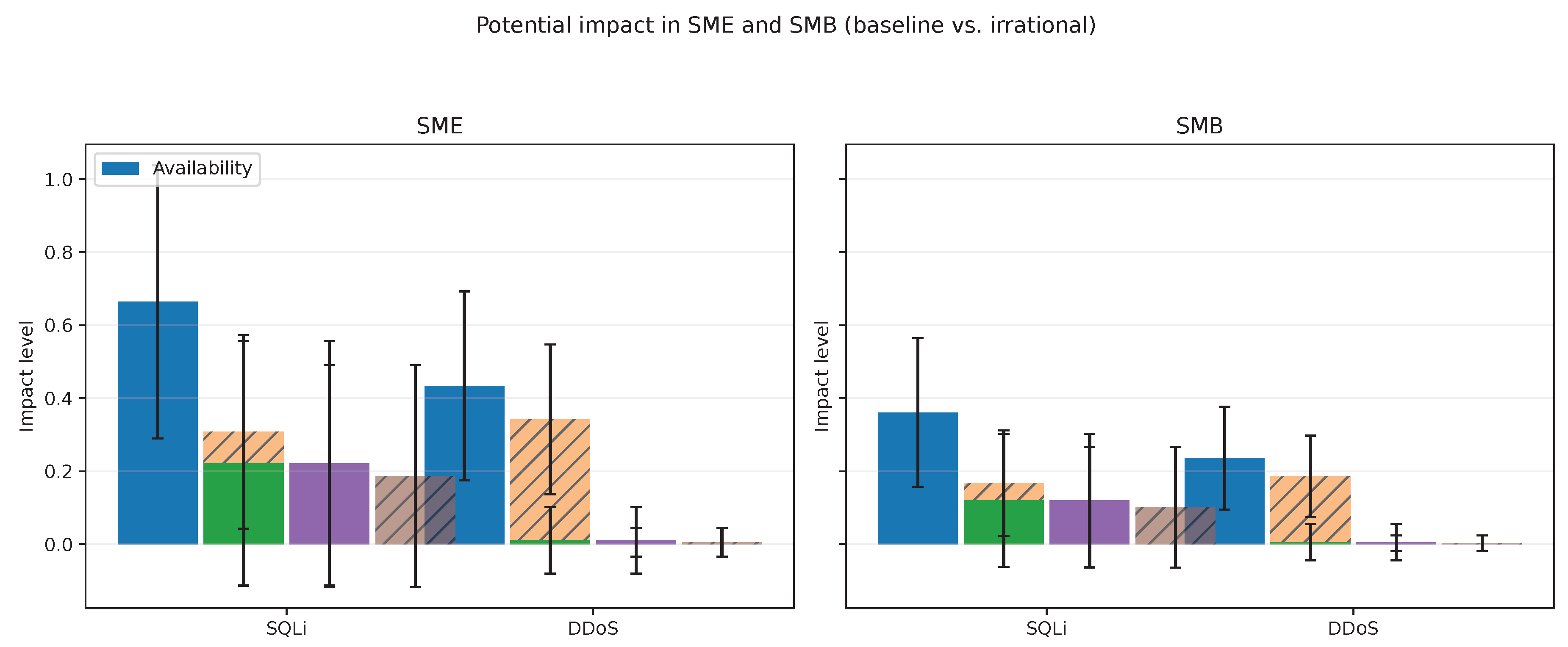
Figure 19.
Impact of irrational attacker behavior on SQLi and DDoS for SME and SMB simulations.
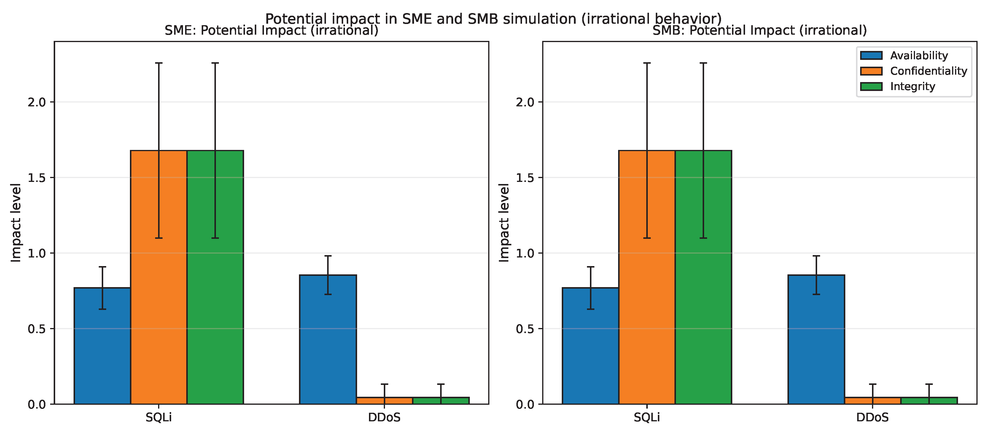
Figure 20.
Behavioral distribution under irrational attack scenarios for SMEs and SMBs.
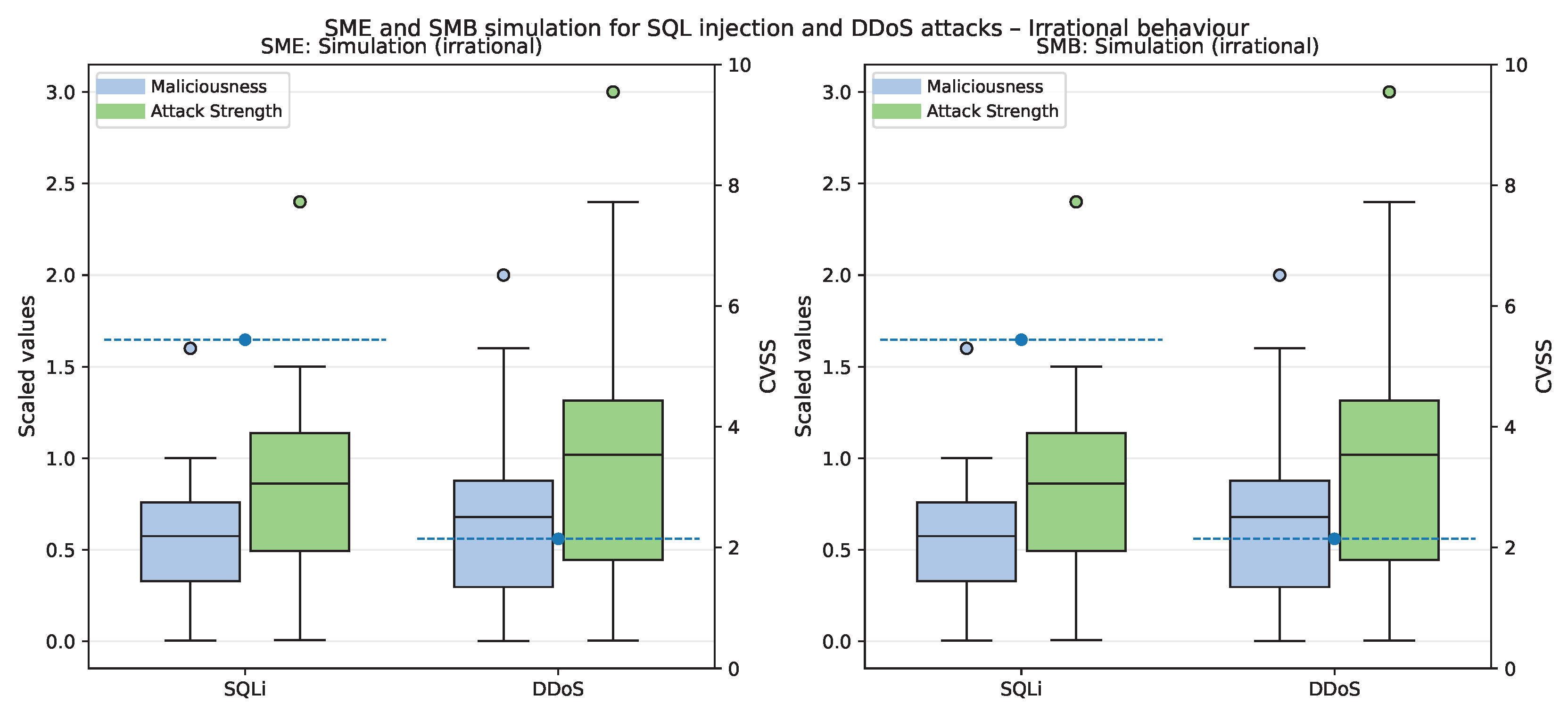
Table 1.
Comparative Analysis of Game-Theoretic Approaches to Digital Forensic Readiness
| Dimension | Our Approach | Nisioti et al. [21] | Karabiyik et al. [23] | Lakhdhar et al. [31] | Wang et al. [38] | Monteiro et al. [36] |
|---|---|---|---|---|---|---|
| Game Model | Non-zero-sum Bimatrix (MNE/PNE) | Bayesian (BNE) | 2×2 Normal-Form | Non-cooperative | ARA (Influence Diagram) | Bayesian (BNE) |
| ATT&CK | ✓Explicit (14 Tactics) | ✓Explicit | × | × | × | × |
| D3FEND | ✓Explicit (6 Families) | × | × | × | × | × |
| Knowledge Coupling | ✓ATT&CK↔D3FEND | Δ ATT&CK + CVSS | Δ Empirical (ForGe) | Δ Internal (CSLib) | Δ Probabilistic (HBN) | Δ CVSS + OpenTelemetry |
| Weighting Method | ✓AHP (10 Experts) | Δ CVSS + SME | Δ Rule-based | Δ Parametric () | Δ Implicit | Δ Scalar Parameters |
| Quantitative Utilities | ✓32 AHP Metrics | ✓Payoff Functions | ✓Payoff Matrix | ✓Parametric | ✓Utility Nodes | ✓Closed-Form |
| Equilibrium | ✓PNE & MNE | ✓BNE | ✓Pure/Mixed NE | ✓Pure/Mixed NE | × ARA | ✓BNE |
| DFR Focus | ✓DFR | Δ Post-mortem | Δ Investigation Efficiency | ✓Forensic Readiness | × Cyber Risk | ✓Forensic Readiness |
| SME/SMB | ✓Explicitly Targeted | Δ Domain-Agnostic | Δ Potential | Δ Applicable | Δ Feasible | Δ Implicit |
| Standardization | Δ ATT&CK, D3FEND, STIX | Δ ATT&CK, STIX, CVSS | Δ Open-Source | Δ CVE/US-CERT | Δ Self-Contained | Δ CVSS, OpenTelemetry |
| Reproducibility | ✓Code, Data, Seeds | Δ Public Inputs, No Code | Δ Code on Request | Δ No Public Code/Data | Δ No Code, Commercial | ✓Benchmark, Repo |
| Key Differentiator | Integrated DFR | Bayesian Anti-Forensics | Tool Selection | Provability Taxonomy | Adversarial Risk Analysis | Microservice Observability |
-
Legend:✓= Fully Addressed; Δ= Partially Addressed; ×= Not Addressed.Abbreviations: AHP (Analytic Hierarchy Process), MNE (Mixed Nash Equilibrium), PNE (Pure Nash Equilibrium), BNE(Bayesian Nash Equilibrium), ARA (Adversarial Risk Analysis), HBN (Hybrid Bayesian Network).Our framework uniquely integrates ATT&CK–D3FEND knowledge with AHP-weighted utilities and explicit SME/SMBtargeting—a combination not found in prior work.
Table 2.
Notation reference for key symbols (see Table A1 in Supplementary Materials for complete listing).
Table 2.
Notation reference for key symbols (see Table A1 in Supplementary Materials for complete listing).
| Symbol | Description |
|---|---|
| Game Structure | |
| Attacker strategy set: , ATT&CK tactics | |
| Defender strategy set: , D3FEND control families | |
| Attacker payoff matrix: , entry | |
| Defender payoff matrix: , entry | |
| Strategies | |
| Attacker pure strategy (ATT&CK tactic) | |
| Defender pure strategy (D3FEND control family) | |
| Attacker mixed strategy: , probability vector over | |
| Defender mixed strategy: , probability vector over | |
| , | Nash equilibrium mixed strategies |
| Utilities and Metrics | |
| Normalized attacker utility: | |
| Normalized defender utility: | |
| AHP weight for attacker metric i: , | |
| AHP weight for defender metric j: , | |
| Attacker DFR metric i value: | |
| Defender DFR metric j value: | |
| Notation Disambiguation | |
| vs. | is a scalar (single entry); is the entire matrix |
| x, y vs. , | x, y are elements/indices; , are mixed-strategy vectors |
Table 10.
Synthetic DFR profiles (before implementation). Illustrative, calibration-based scenarios; not field measurements.
Table 10.
Synthetic DFR profiles (before implementation). Illustrative, calibration-based scenarios; not field measurements.
| File No. | L | I | D | VDCC | E | IR | DR | NF | STd | LR | A | C | T | R | V | Pd |
|---|---|---|---|---|---|---|---|---|---|---|---|---|---|---|---|---|
| case1 | 0.5 | 0.6 | 0.3 | 0.4 | 0.5 | 0.6 | 0.2 | 0.5 | 0.2 | 0.6 | 0.7 | 0.2 | 0.6 | 0.1 | 0.2 | 0.4 |
| case2 | 0.1 | 0.2 | 0.7 | 0.6 | 0.1 | 0.2 | 0.6 | 0.1 | 0.6 | 0.4 | 0.2 | 0.6 | 0.2 | 0.1 | 0.6 | 0.5 |
| case3 | 0.6 | 0.1 | 0.6 | 0.5 | 0.6 | 0.4 | 0.2 | 0.2 | 0.6 | 0.1 | 0.6 | 0.1 | 0.2 | 0.6 | 0.1 | 0.6 |
| case4 | 0.7 | 0.2 | 0.2 | 0.7 | 0.2 | 0.6 | 0.4 | 0.6 | 0.2 | 0.1 | 0.2 | 0.6 | 0.1 | 0.2 | 0.6 | 0.2 |
| case5 | 0.7 | 0.6 | 0.3 | 0.5 | 0.6 | 0.7 | 0.4 | 0.2 | 0.6 | 0.3 | 0.6 | 0.2 | 0.1 | 0.6 | 0.2 | 0.3 |
| case6 | 0.5 | 0.7 | 0.5 | 0.7 | 0.5 | 0.4 | 0.6 | 0.6 | 0.3 | 0.2 | 0.6 | 0.1 | 0.6 | 0.2 | 0.4 | 0.6 |
| case7 | 0.4 | 0.6 | 0.3 | 0.6 | 0.7 | 0.6 | 0.2 | 0.2 | 0.7 | 0.6 | 0.2 | 0.7 | 0.6 | 0.2 | 0.5 | 0.4 |
| case8 | 0.1 | 0.2 | 0.6 | 0.5 | 0.6 | 0.2 | 0.5 | 0.4 | 0.2 | 0.6 | 0.1 | 0.2 | 0.6 | 0.7 | 0.6 | 0.2 |
| case9 | 0.6 | 0.3 | 0.2 | 0.6 | 0.2 | 0.3 | 0.6 | 0.6 | 0.4 | 0.2 | 0.6 | 0.3 | 0.2 | 0.6 | 0.2 | 0.5 |
| case10 | 0.5 | 0.6 | 0.3 | 0.2 | 0.6 | 0.2 | 0.7 | 0.2 | 0.5 | 0.6 | 0.2 | 0.4 | 0.2 | 0.6 | 0.5 | 0.2 |
Table 11.
Synthetic DFR profiles (after implementation). Illustrative, calibration-based scenarios; not field measurements. Profiles generated using targeted framework uplift with coupling constraints (see Section 4.3.1).
Table 11.
Synthetic DFR profiles (after implementation). Illustrative, calibration-based scenarios; not field measurements. Profiles generated using targeted framework uplift with coupling constraints (see Section 4.3.1).
| File No. | L | I | D | VDCC | E | IR | DR | NF | STd | LR | A | C | T | R | V | Pd |
|---|---|---|---|---|---|---|---|---|---|---|---|---|---|---|---|---|
| case1 | 0.8 | 0.8 | 0.7 | 0.9 | 0.8 | 0.8 | 0.7 | 0.9 | 0.7 | 0.6 | 0.8 | 0.7 | 0.8 | 0.7 | 0.7 | 0.7 |
| case2 | 0.9 | 0.8 | 0.9 | 0.8 | 0.7 | 0.9 | 0.7 | 0.8 | 0.6 | 0.7 | 0.7 | 0.8 | 0.7 | 0.6 | 0.6 | 0.8 |
| case3 | 0.8 | 0.7 | 0.8 | 0.9 | 0.8 | 0.9 | 0.8 | 0.9 | 0.7 | 0.8 | 0.8 | 0.7 | 0.7 | 0.7 | 0.8 | 0.7 |
| case4 | 0.8 | 0.9 | 0.9 | 0.8 | 0.7 | 0.9 | 0.9 | 0.8 | 0.7 | 0.7 | 0.7 | 0.8 | 0.7 | 0.7 | 0.6 | 0.8 |
| case5 | 0.7 | 0.7 | 0.9 | 0.7 | 0.8 | 0.9 | 0.7 | 0.9 | 0.8 | 0.8 | 0.7 | 0.7 | 0.6 | 0.8 | 0.7 | 0.7 |
| case6 | 0.7 | 0.8 | 0.8 | 0.9 | 0.7 | 0.8 | 0.6 | 0.9 | 0.6 | 0.7 | 0.6 | 0.8 | 0.7 | 0.9 | 0.7 | 0.7 |
| case7 | 0.8 | 0.7 | 0.9 | 0.7 | 0.6 | 0.9 | 0.8 | 0.9 | 0.7 | 0.8 | 0.7 | 0.7 | 0.8 | 0.7 | 0.8 | 0.8 |
| case8 | 0.7 | 0.6 | 0.9 | 0.8 | 0.8 | 0.9 | 0.8 | 0.8 | 0.8 | 0.7 | 0.7 | 0.8 | 0.7 | 0.6 | 0.8 | 0.7 |
| case9 | 0.9 | 0.7 | 0.8 | 0.7 | 0.7 | 0.9 | 0.7 | 0.8 | 0.7 | 0.8 | 0.8 | 0.7 | 0.6 | 0.7 | 0.7 | 0.7 |
| case10 | 0.8 | 0.8 | 0.9 | 0.7 | 0.7 | 0.9 | 0.8 | 0.7 | 0.7 | 0.8 | 0.7 | 0.7 | 0.8 | 0.8 | 0.6 | 0.8 |
Table 12.
Simulation Results Based on Evolutionary Game Theory
| Resources | Defenders | Attackers | Scenario | Final Value | Avg. Attacker Strategy | Avg. Defender Strategy | Avg. Readiness |
|---|---|---|---|---|---|---|---|
| 1 | 10 | 5 | a | 0.56 | 0.84 | – | 0.00 |
| 1 | 15 | 5 | b | 0.52 | 0.94 | – | 0.00 |
| 1 | 25 | 5 | c | 0.61 | 0.69 | – | 0.00 |
| 3 | 10 | 5 | d | 0.96 | 0.58 | – | 0.00 |
| 3 | 25 | 5 | f | 1.00 | 1.00 | – | 0.00 |
| 5 | 15 | 5 | h | 0.91 | 0.75 | – | 0.03 |
Table 13.
Simulation results (mean ± 95% CI; trials per setting).
| Low | Medium | High | |
|---|---|---|---|
| Attack success rate | 0.25 ± 0.0038 | 0.53 ± 0.0044 | 0.75 ± 0.0038 |
| Evidence collection rate | 0.93 ± 0.0022 | 0.96 ± 0.0017 | 0.94 ± 0.0021 |
Table 14.
Simulation results of attack success rate for SME and SMB organizations.
| ID | SME | SMB | Impact metrics | |||||||||||
|---|---|---|---|---|---|---|---|---|---|---|---|---|---|---|
| Type | Malic. | Str. | Impact | CVSS | Type | Malic. | Str. | Impact | CVSS | Workload | Avail. | Conf. | Integ. | |
| 0 | DDoS | 0.75 | 1.12 | High | 7 | DDoS | 0.75 | 1.12 | High | 7 | 1.125 | 0.8 | 0 | 0 |
| 1 | SQLI | 0.75 | 1.12 | High | 9 | SQLI | 0.75 | 1.12 | High | 9 | 2.7 | 2.58 | 7.2 | 7.2 |
| 2 | DDoS | 0.75 | 1.12 | Med | 0 | DDoS | 0.75 | 1.12 | Med | 0 | 1.125 | 0.96 | 0 | 0 |
| 3 | SQLI | 0.75 | 1.12 | High | 9 | SQLI | 0.75 | 1.12 | High | 9 | 1.125 | 1.005 | 7.2 | 7.2 |
| 4 | DDoS | 0.75 | 1.12 | Low | 0 | DDoS | 0.75 | 1.12 | Low | 0 | 1.125 | 0.96 | 0 | 0 |
| 5 | SQLI | 0.75 | 1.12 | Med | 7 | SQLI | 0.75 | 1.12 | Med | 7 | 2.7 | 2.58 | 2.8 | 2.8 |
Table 15.
Simulation result of attack success rate—irrational behavior.
| ID | SME | SMB | Impact metrics | |||||||||||
|---|---|---|---|---|---|---|---|---|---|---|---|---|---|---|
| Type | Malic. | Str. | Impact | CVSS | Type | Malic. | Str. | Impact | CVSS | Workload | Avail. | Conf. | Integ. | |
| 0 | SQLI | 0.49 | 0.73 | Med | 7 | SQLI | 0.49 | 0.73 | Med | 7 | 0.73 | 0.61 | 2.8 | 2.8 |
| 1 | DDoS | 0.75 | 1.12 | High | 7 | DDoS | 0.75 | 1.12 | High | 7 | 1.12 | 0.80 | 0 | 0 |
| 2 | DDoS | 0.80 | 1.21 | High | 7 | DDoS | 0.80 | 1.21 | High | 7 | 1.21 | 0.80 | 0 | 0 |
| 3 | SQLI | 0.16 | 0.24 | High | 9 | SQLI | 0.16 | 0.24 | High | 9 | 0.24 | 0.12 | 7.2 | 7.2 |
| 4 | SQLI | 0.58 | 0.87 | High | 9 | SQLI | 0.58 | 0.87 | High | 9 | 2.45 | 2.33 | 7.2 | 7.2 |
| 5 | DDoS | 0.84 | 1.26 | High | 7 | DDoS | 0.84 | 1.26 | High | 7 | 2.84 | 0.80 | 0 | 0 |
Disclaimer/Publisher’s Note: The statements, opinions and data contained in all publications are solely those of the individual author(s) and contributor(s) and not of MDPI and/or the editor(s). MDPI and/or the editor(s) disclaim responsibility for any injury to people or property resulting from any ideas, methods, instructions or products referred to in the content. |
© 2025 by the authors. Licensee MDPI, Basel, Switzerland. This article is an open access article distributed under the terms and conditions of the Creative Commons Attribution (CC BY) license (http://creativecommons.org/licenses/by/4.0/).
Copyright: This open access article is published under a Creative Commons CC BY 4.0 license, which permit the free download, distribution, and reuse, provided that the author and preprint are cited in any reuse.


