Submitted:
13 October 2025
Posted:
14 October 2025
You are already at the latest version
Abstract
This survey paper presents a comprehensive review of convolution operations in Convolutional Neural Networks (CNNs). We trace the evolution of convolutions from their mathematical foundations to their implementation in modern deep learning architectures. We examine various types of convolutions, their properties, and their applications across different domains, including image processing, audio analysis, natural language processing, and scientific applications. Additionally, we discuss the biological inspiration behind CNNs, key architectural innovations, and emerging trends in the field. This paper serves as a resource for researchers and practitioners interested in understanding the fundamental building blocks of CNNs and their continuing evolution.
Keywords:
convolutional neural networks
; deep learning
; computer vision
; convolution operations
; CNN architectures
1. Introduction
1.1. Definition of Convolution and Its Importance in CNNs
Imagine trying to find your friend’s face in a crowded photograph. Your brain doesn’t analyze every pixel individually—instead, it looks for familiar patterns like the curve of a smile or the shape of an eye. Convolutional Neural Networks (CNNs) work similarly, using mathematical operations called convolutions to automatically detect meaningful patterns in visual data.
In the context of CNNs, convolution enables networks to detect local features—such as edges, textures, and shapes—by sliding small filters (kernels) across input images and computing weighted sums at each position.
This seemingly simple operation has profound implications for artificial intelligence. The unique power of CNNs lies in their ability to automatically learn relevant visual patterns from data, rather than requiring human experts to manually design feature detectors. This capability has revolutionized computer vision by enabling machines to achieve human-level or superhuman performance on many visual recognition tasks. The breakthrough moment came in 2015 when Microsoft’s ResNet achieved a 3.57% error rate on ImageNet, surpassing human-level performance (estimated at 5.1%). In medical applications, CNNs have demonstrated superhuman diagnostic accuracy, with systems achieving 95% accuracy in detecting diabetic retinopathy compared to 91% for ophthalmologists, and matching dermatologist-level performance in skin cancer classification [1,2].
Building on these successes, CNNs have become fundamental tools across numerous critical applications including image classification, object detection, face recognition, medical image analysis, autonomous driving systems, video surveillance, natural language processing, speech recognition, recommender systems, anomaly detection, augmented reality, satellite image interpretation, handwriting recognition, pose estimation, and scene segmentation [3,4]. As of 2024, CNNs process the vast majority of images uploaded to major social media platforms, with Facebook alone running inference on billions of images daily. CNNs serve as the cornerstone of modern computer vision systems and are extensively deployed in leading technology companies including Google, Meta, Microsoft, and NVIDIA for image perception, computer vision, and artificial intelligence applications.
The evolution of CNN architectures has been instrumental in enabling breakthrough applications across multiple domains. Starting with LeNet-5’s pioneering work in digit recognition, successive architectural innovations like AlexNet’s deep learning revolution, VGGNet’s systematic depth exploration, GoogLeNet’s efficient multi-scale processing, ResNet’s ultra-deep networks, DenseNet’s feature reuse paradigms, and MobileNet’s mobile-optimized designs have each contributed unique solutions to computational and performance challenges. This progression has yielded dramatic improvements: error rates on ImageNet dropped from 26% (pre-AlexNet) to 1.5% (current state-of-the-art), while computational efficiency improved by 180× between AlexNet and EfficientNet for comparable accuracy levels [5].
These architectural advances have collectively enabled modern applications ranging from autonomous vehicle perception systems and medical diagnostic imaging to real-time object detection in smartphones and large-scale content moderation systems. Figure 1 illustrates this remarkable progression of CNN architectures, showing how each innovation built upon previous work to push the boundaries of what was computationally feasible and practically deployable.
Despite their success, CNNs face significant challenges including substantial data requirements (typically millions of labeled examples), high computational costs (training large-scale vision models can cost millions of dollars), limited interpretability, and emerging competition from Vision Transformers which have achieved state-of-the-art results on several benchmarks. These challenges drive ongoing research into more efficient architectures, few-shot learning approaches, and hybrid models that combine the strengths of different architectural paradigms [6].
As we explore CNNs’ mathematical foundations, historical development, architectural innovations, and practical applications, we gain deeper insight into how this technology has transformed artificial intelligence and continues to evolve across diverse domains from medical imaging to autonomous systems.
1.2. Mathematical Foundations of Convolution
To understand how CNNs work, we must first understand convolution itself. Think of convolution as a way of “mixing" two signals or images together to create a new one that captures how they interact.
1.2.1. The Simple Intuition
Consider a simple example: you’re listening to music in a large cathedral. The original song (our input signal) gets "mixed" with the cathedral’s acoustic properties (our filter) to produce what you actually hear (the output). The convolution operation mathematically describes this mixing process. For instance, when processing audio, the input signal might be a recorded voice, the filter represents a room’s echo pattern, and the convolution produces what you would actually hear in that space.
In image processing, convolution works similarly. Imagine you have a photograph and a small "template" that detects horizontal edges. When you slide this template across every position in the photograph, computing how well it matches at each location, you’re performing convolution. The result is a new image that highlights all the horizontal edges in the original.
1.2.2. Historical Development and Mathematical Formalization
While this intuition helps us understand what convolution does, the mathematical formalization of this concept has a rich history spanning over two centuries. The operation emerged gradually through the work of several mathematicians, each contributing essential pieces to our modern understanding.
Leonhard Euler (1707-1783) laid crucial groundwork in the 1760s through his work on integral calculus and differential equations. In his “Institutionum Calculi Integralis" (1768), Euler studied second-order partial differential equations that involved operations mathematically equivalent to convolution, though the term itself would not appear for another century [7].
Pierre-Simon Laplace (1749-1827) advanced these ideas significantly in 1778 through his work on probability theory and the Laplace transform. His analysis of how probability distributions combine when random variables are added provided crucial insights into convolution’s statistical interpretation [8].
Joseph Fourier (1768-1830) formalized the deep connection between convolution and frequency domain analysis in the early 19th century. His work demonstrated that convolution in the time domain corresponds to multiplication in the frequency domain, establishing the mathematical foundation for modern signal processing [9].
The mathematical operation existed for over a century before receiving its modern name. The term “convolution" wasn’t introduced until 1897 by mathematicians studying integral equations, and didn’t become standard English mathematical terminology until 1937 [10].
These mathematical foundations became practically implementable with the advent of digital computing in the mid-20th century. The Fast Fourier Transform algorithm (1965) made frequency-domain convolution computationally feasible, while the development of digital signal processors in the 1980s enabled real-time convolution operations. This computational infrastructure was essential for the eventual emergence of CNNs, as it provided both the theoretical framework and practical tools needed to implement convolution operations in neural networks.
1.2.3. Formal Mathematical Definition
Having traced convolution’s historical development, we now turn to its precise mathematical formulation. For continuous signals, convolution mathematically combines two functions f and g to produce a third function that expresses how the shape of one is modified by the other:
where f represents the input signal, g represents the system’s impulse response (or filter), and gives the system’s output at time t.
Intuitive Interpretation: At each time t, we compute the output by taking the input signal f, “flipping" the filter g around the origin (the term reverses the filter’s direction), sliding it to position t, multiplying the overlapping portions pointwise, and integrating the result. This flipping operation means that if were the original filter values, we would use them in the order when computing the convolution. This process captures how the filter modifies the input signal at every moment.
For discrete signals (like digital images), the convolution becomes a summation:
1.2.4. 2D Convolution for Image Processing
The transition from one-dimensional signals to two-dimensional images requires extending the convolution operation across both spatial dimensions. Just as 1D convolution slides a kernel along a temporal or sequential axis, 2D convolution slides a kernel across both the height and width of an image, enabling detection of spatial patterns like edges, corners, and textures.
Images are two-dimensional grids of pixel values, requiring 2D convolution. For an input image and a filter kernel , the 2D convolution is defined as:
where the output represents the feature map value at position .
To illustrate this mathematical operation concretely, consider Figure 2 which demonstrates the step-by-step process of 2D convolution. In this visualization, a small kernel (shown in blue) systematically moves across a larger input image to produce an output feature map. This process embodies the essence of how CNNs detect local patterns within images.
The convolution operation begins with the kernel positioned at the top-left corner of the input image. At this position, each value in the kernel is multiplied by the corresponding pixel value it overlaps in the input image. These products are then summed together to produce a single output value, which becomes the first element of our feature map. This operation captures how well the pattern encoded in the kernel matches the local region of the input.
As the kernel slides horizontally and vertically across the input (with the green highlighting indicating the current region being processed), this multiplication-and-summation process repeats at each position. The systematic sliding ensures that the kernel examines every possible location in the input image, searching for the pattern it encodes. Each computed sum represents the strength of the pattern’s presence at that particular location.
This sliding window approach directly implements Equation 3, where the indices determine the kernel’s position, and the summation over m and n performs the element-wise multiplication and accumulation. The resulting feature map effectively creates a “heat map" showing where and how strongly the kernel’s pattern appears throughout the input image. This fundamental operation, repeated with many different learned kernels, enables CNNs to build rich representations of visual data.
Technical Note on Cross-Correlation: Modern CNNs actually implement cross-correlation rather than true mathematical convolution. In true convolution, the kernel would be flipped both horizontally and vertically before sliding across the image (mathematically, this would replace with in Equation 3). Cross-correlation omits this flipping step and slides the kernel as-is. Since CNN filters are learned through backpropagation rather than designed analytically, this distinction has no practical impact—the network simply learns the appropriate kernel weights regardless of whether the operation technically involves flipping. However, mathematical rigor requires acknowledging this difference [11].
1.2.5. Tensor Formulation for Multi-Channel Images
Real images have multiple color channels (RGB), requiring us to extend our formulation to handle tensor operations. We must also introduce two critical parameters that control the convolution’s spatial behavior: padding (additional border pixels added to preserve spatial dimensions and control boundary effects) and stride (the step size of the kernel’s movement across the input, which controls downsampling).
For input with C channels and filter bank producing K feature maps:
where is the bias term for the k-th output channel, and is the output feature map with dimensions:
where P is the padding size and S is the stride value.
Understanding this mathematical formulation is crucial for practitioners because it directly impacts model design decisions. The choice of kernel size F determines the receptive field (the area of input that influences one output pixel) and computational cost, padding P controls spatial dimension preservation (critical for skip connections in architectures like U-Net), and stride S affects the downsampling rate and feature map resolution. These parameters fundamentally influence model capacity, memory requirements, and the types of patterns the network can detect [12].
This mathematical foundation—from Euler’s differential equations to modern tensor operations—provides the theoretical framework upon which all CNN architectures are built, enabling the pattern recognition capabilities that have revolutionized computer vision and artificial intelligence.
1.3. Biological Inspiration: Neurons, Receptive Fields, and Feature Extraction
Having established the mathematical foundations of convolution, we now examine the biological principles that inspired CNN architectures. The underlying principles of CNNs trace their roots back to the groundbreaking experiments of Hubel and Wiesel, who discovered that visual information is processed hierarchically in the visual cortex of mammals. They found that simple cells in primary visual areas like V1 respond to basic structures like lines and edges, while complex cells in higher-order regions respond to more abstract entities like facial structure or entire objects [13].
Hubel and Wiesel’s experiments, conducted on anesthetized cats and monkeys, involved inserting microelectrodes into individual neurons in the visual cortex while presenting various visual stimuli. They discovered that neurons in V1 responded maximally to bars of light at specific orientations and positions in the visual field. Moving deeper into the visual system, they found neurons with progressively larger receptive fields that responded to more complex patterns. This hierarchical organization, where simple features are combined to form complex representations, became the fundamental principle underlying CNN architecture design.
This hierarchical visual processing inspired CNN designs, with increasingly complex visual features extracted by each layer. Figure 3 illustrates this parallel by showing how early CNN layers detect low-level patterns such as edges and lines, mid-level layers identify object parts like eyes and noses, and high-level layers respond to entire faces and categories, mirroring the progression observed in biological visual systems.
Later, researchers such as Kunihiko Fukushima developed the Neocognitron [14], one of the first models to computationally emulate this hierarchical structure using the concepts of local receptive fields and shared weights. These ideas became core principles in today’s CNNs, continuing into Yann LeCun’s LeNet [15] and later VGG architectures [16] where deeper representations learned more abstract patterns through stacking multiple convolutional layers.
Both structurally and functionally, CNNs are biologically motivated. Yamins and DiCarlo have demonstrated that deep CNNs can successfully model the ventral visual pathway of the brain, the pathway responsible for object recognition [17]. Through their work, they showed evidence of how CNN activation in different layers corresponds well with primate visual cortex responses, suggesting a correspondence between artificial and biological vision systems. Yosinski’s work [18] has also delved into the internal representations of features by CNNs, revealing what individual layers “see" and helping develop methods for interpreting and visualizing learned representations [19,20].
However, CNNs capture only a fraction of the biological visual system’s capabilities. Biological vision incorporates attention mechanisms that dynamically focus processing on relevant regions, top-down feedback that uses context and expectations to guide perception, and rapid adaptation to new visual concepts from few examples. The brain also performs continuous online learning, integrates multimodal sensory information, and maintains stable perception despite constant eye movements—capabilities that remain challenging for current CNN architectures.
Despite these correspondences, important limitations exist in the biological analogy. CNNs process static images in a single feedforward pass, while biological vision involves recurrent processing with multiple feedback loops. CNNs require millions of labeled examples for training, whereas humans learn new visual concepts from single examples. Additionally, CNNs are vulnerable to adversarial examples—imperceptible perturbations that cause misclassification—suggesting fundamental differences in how artificial and biological systems represent visual information [21].
Current research aims to bridge this gap through biologically-inspired improvements including spiking neural networks that more accurately model neural dynamics, feedback connections that enable top-down processing, and attention mechanisms inspired by visual saccades. These advances may lead to more robust, efficient, and adaptable vision systems that better match biological performance in challenging real-world conditions.
2. Fundamentals of Convolutions
2.1. What Convolution Actually Does in Neural Networks
In neural networks, convolution serves as a sophisticated feature extractor that automatically learns relevant patterns from data through a systematic sliding window operation. Think of each kernel as a small “pattern template" that slides across the input image (as illustrated in Figure 2), checking how well each local region matches the pattern it has learned to detect.
The convolution operation processes input data by applying a kernel (filter) across the input tensor, computing dot products between the kernel and local regions, and generating feature maps that highlight the spatial locations of detected patterns. When the kernel encounters a region that closely matches its learned pattern, it produces a high response value. When the local region differs significantly from the pattern, the response is low. This creates a “heat map" showing where the kernel’s specific pattern appears throughout the image.
Conceptually, each kernel acts like a reusable “pattern detector." As the kernel slides across the input, its response at a location is high when the local patch resembles the learned pattern and low otherwise, producing a heat map (feature map) of where that pattern occurs. During training, backpropagation adjusts the kernel weights so that the detector becomes highly responsive to task-relevant cues (e.g., edges, corners, textures) without manual feature engineering.
The practical impact of this automatic feature learning capability has proven superior to classical computer vision approaches across diverse domains, from medical imaging where pathological patterns vary significantly across patients, to autonomous driving where environmental conditions create unpredictable visual variations. The convolution operation’s inherent ability to learn task-specific feature detectors has revolutionized pattern recognition by eliminating the feature engineering bottleneck that previously limited computer vision applications.
2.2. Core Properties That Make Convolution Powerful
Before exploring the mathematical variations of convolution, we must understand the three fundamental properties that make convolutional operations so effective for visual pattern recognition: translation invariance, weight sharing, and hierarchical feature learning. These properties work together to create robust, efficient, and scalable neural network architectures.
2.2.1. Translation Invariance: The Foundation of Robust Pattern Recognition
Translation invariance represents one of convolution’s most powerful properties, enabling feature recognition regardless of spatial position within the input. This property emerges naturally from the convolution operation’s weight sharing mechanism, where the same kernel is applied across all spatial locations. More precisely, standard convolutions are translation equivariant: shifting the input shifts the feature maps by the same amount. True invariance is typically obtained after spatial pooling (a downsampling operation that aggregates local features, discussed in detail in subsequent sections) or global average pooling, which discards exact location while preserving the presence of features.
To understand this concept, imagine teaching a CNN to recognize cats. With translation invariance, the network can detect a cat whether it appears in the top-left corner, center, or bottom-right of an image. The same kernel that learned to detect “cat ears" will respond equally well regardless of where those ears appear in the image.
The practical implications of translation invariance extend far beyond theoretical elegance. In medical imaging, tumors can appear anywhere within an organ, yet CNNs maintain consistent detection performance regardless of lesion location. Similarly, in satellite imagery analysis, CNNs can identify agricultural fields, urban structures, or natural disasters independent of their geographic coordinates within the image frame. This spatial robustness eliminates the need for position-specific training, dramatically reducing the complexity of dataset preparation and model development.
The biological inspiration for translation invariance stems from receptive field studies in mammalian visual cortex, where neurons respond to specific visual patterns regardless of their retinal position. This neural mechanism enables animals to recognize objects across varying viewpoints and positions, a capability that CNNs successfully emulate through mathematical convolution operations.
Limits and failure cases: Equivariance breaks at image boundaries (padding effects), with striding (aliasing), and under strong scale or rotation changes. Pooling confers only coarse invariance and may discard spatial detail needed for fine localization. In practice, data augmentation (shifts, crops) and antialiased downsampling choices help preserve robustness, while tasks that need exact layout (e.g., documents) often retain positional signals.
However, perfect translation invariance presents limitations in applications where spatial context carries semantic meaning. Document analysis requires understanding reading order and spatial layout, while certain medical diagnoses depend on anatomical position relationships. Modern designs therefore combine convolutional features with mechanisms that preserve or inject position information to balance robustness with spatial specificity [6].
2.2.2. Weight Sharing: Computational Efficiency Through Parameter Reuse
While translation invariance provides robustness to spatial position, another fundamental property enables CNNs to achieve this efficiently. Weight sharing in CNNs achieves remarkable computational efficiency by applying the same kernel parameters across all spatial locations, fundamentally changing the parameter scaling relationship compared to fully connected architectures. This concept represents one of the most elegant solutions in deep learning: instead of learning separate parameters for every possible input location, CNNs learn one set of parameters (the kernel) and reuse it everywhere.
To appreciate the efficiency gains, consider a typical input image. A fully connected layer requires approximately 150 million parameters to connect to 1000 output neurons, while a convolutional layer with 64 filters of size requires only 1,728 parameters—a reduction factor of nearly 87,000. (Including one bias per filter yields 64 additional parameters.)
This dramatic parameter reduction enables several critical advantages in deep learning applications. Reduced parameter counts directly translate to lower memory requirements, enabling deployment on resource-constrained devices from smartphones to embedded systems. Additionally, fewer parameters reduce overfitting risk, particularly beneficial when training data is limited, while simultaneously decreasing computational requirements for both training and inference phases.
The mathematical foundation of weight sharing ensures that each filter learns a specific pattern applicable across different spatial regions. This approach proves particularly effective for natural images where visual patterns—edges, textures, and shapes—appear consistently across different locations. However, weight sharing can limit representational capacity when spatial location carries important semantic information, leading to architectural innovations like attention mechanisms that selectively break translation invariance.
Across architectures, parameter efficiency is further improved by grouped and depthwise separable convolutions, which factorize standard convolutions into cheaper operations. Grouped convolutions (e.g., ResNeXt) limit channel mixing to groups, while depthwise separable convolutions (e.g., MobileNet) split spatial filtering (depthwise) from channel mixing (pointwise), yielding large FLOP and parameter savings with modest accuracy trade-offs [22,23].
Weight sharing’s biological motivation derives from cortical organization principles, where neurons with similar receptive field properties are arranged in regular patterns across the visual cortex. This neural architecture suggests that efficient visual processing naturally employs shared computational elements, providing evolutionary validation for CNN design principles.
When weight sharing is suboptimal—for layout-sensitive tasks, charts, diagrams, or geospatial maps—architectures often augment convolutions with attention mechanisms to let the model condition on absolute or relative position while retaining the efficiency of shared filters.
2.2.3. Hierarchical Feature Learning: From Edges to Objects
Translation invariance and weight sharing explain how CNNs process spatial information efficiently, but they don’t explain how CNNs build understanding from simple to complex. This capability emerges from a third core property: hierarchical feature learning. CNNs learn features hierarchically: early layers respond to simple structures (oriented edges, color contrasts), middle layers compose these into textures and parts (eyes, wheels), and deeper layers respond to whole objects or categories. This progression emerges because stacking small receptive fields increases the effective receptive field, allowing deeper units to integrate broader context.
Think of this like learning to read: first you recognize individual letters (simple features), then common letter combinations (textures and patterns), then words (parts), and finally complete sentences (objects). Each level builds upon the previous one, creating increasingly sophisticated understanding.
For n stacked layers (stride 1, no dilation), the theoretical receptive field grows to , enabling large-context reasoning without large kernels. This mathematical property allows CNNs to capture global image context through deep architectures rather than requiring enormous kernels that would be computationally prohibitive.
Empirical visualizations corroborate this organization: deconvolution/activation inversion shows a layer-wise evolution from edges to parts to objects [19]. Neural response studies also report strong alignment between CNN layer activations and ventral-stream responses in primates, suggesting that hierarchical composition is a useful inductive bias for object recognition [17].
The practical advantages of hierarchical feature learning extend beyond biological plausibility to computational efficiency and generalization capability. By learning reusable feature components at each hierarchical level, CNNs achieve remarkable parameter efficiency compared to non-hierarchical approaches. Additionally, hierarchical representations enable effective transfer learning, where features learned on one task generalize to related tasks, dramatically reducing training requirements for new applications.
2.3. Dimensional Variants: Adapting Convolution to Data Structure
Having established the core principles—translation invariance, weight sharing, and hierarchical learning—we now explore how these principles adapt to different data structures through dimensional variants of convolution. Each variant maintains the fundamental properties of weight sharing and local feature detection while accommodating specific characteristics of different data types.
2.3.1. 1D Convolutions for Sequential Data Processing
One-dimensional convolutions extend convolution principles to sequential data domains including time series, audio signals, and textual sequences. Instead of sliding across spatial dimensions like images, 1D kernels slide along the temporal or sequential dimension, capturing local patterns and dependencies over time.
The fundamental operation involves sliding a 1D kernel across the temporal dimension, computing weighted combinations that capture local temporal patterns. For a 1D input signal and kernel of length K, the convolution produces output , where each output value represents the presence of the kernel’s encoded pattern at that temporal position. (In causal settings, indices are shifted so predictions depend only on past samples.)
The historical development of 1D convolutions traces to digital signal processing applications in telecommunications and audio engineering during the 1960s and 1970s. Early applications focused on filtering and noise reduction in communication systems, but the integration with neural networks occurred much later. In modern deep learning, 1D CNNs are competitive on tasks driven by local motifs (e.g., n-gram-like text patterns or short-time spectral cues) and are attractive when low latency and parallelism are important, whereas architectures designed for long-range dependencies (e.g., self-attention) may perform better when very long contexts dominate.
Padding strategies in 1D convolutions directly control temporal coverage and output sequence length. Causal padding ensures that predictions depend only on past information, crucial for real-time applications, while symmetric padding enables bi-directional temporal context integration. Stride selection significantly impacts temporal resolution and computational efficiency, with larger strides trading temporal precision for processing speed.
Applications where 1D convolutions excel include audio classification where local spectral patterns indicate phonemes or musical elements, financial time series analysis where short-term price movements reveal market patterns, and sensor data processing where temporal patterns indicate system states or anomalies. However, 1D convolutions struggle with long-range temporal dependencies, requiring either very large kernels or deep architectures to capture extended temporal relationships. Dilated (atrous) 1D convolutions expand receptive fields without large parameter counts, providing a practical compromise for mid-range contexts.
2.3.2. 2D Convolutions: The Foundation of Computer Vision
Two-dimensional convolutions represent the cornerstone of modern computer vision, operating on spatial data structures including grayscale images, color photographs, and multi-spectral imagery. The 2D convolution operation systematically applies kernels across both spatial dimensions, capturing local spatial features such as edges, textures, corners, and more complex geometric patterns. Each kernel learns to detect specific spatial patterns, with the collection of learned kernels in a layer providing diverse feature detection capabilities that enable robust visual pattern recognition.
The mathematical formulation of 2D convolution extends naturally from 1D operations but introduces additional complexity in boundary handling and computational optimization. For input image and kernel , the basic operation follows Equation 3 from Section 1. The output feature map dimensions depend critically on padding and stride parameters according to the formula (see Equation 5), where proper parameter selection maintains desired spatial resolution throughout the network architecture.
Padding strategies in 2D convolutions serve multiple purposes beyond dimension preservation. Zero padding, the most common approach, introduces boundary artifacts that can be beneficial for edge detection tasks, while reflection padding better preserves natural image statistics near boundaries. The choice of padding strategy can significantly impact performance in tasks requiring precise spatial localization, such as medical image segmentation where tissue boundaries must be accurately preserved.
The transformative impact of 2D convolutions became evident with AlexNet’s 2012 ImageNet victory, demonstrating that learned convolutional features could surpass decades of hand-crafted computer vision research. This breakthrough catalyzed widespread adoption across industries, from smartphone camera applications enabling real-time object recognition to medical imaging systems providing automated diagnostic assistance. These gains reflect how 2D convolutions align with natural-image statistics (local correlations, repeated motifs) and exploit weight sharing to learn compact, transferable filters.
Modern systems also accelerate 2D convolutions with FFT- and Winograd-based algorithms for large and small kernels, respectively, enabling real-time processing on edge devices and efficient cloud-scale inference [24].
2.3.3. 3D Convolutions: Spatiotemporal and Volumetric Processing
Three-dimensional convolutions extend convolution operations to volumetric and spatiotemporal data, enabling analysis of medical imaging volumes, video sequences, and scientific datasets with inherent 3D structure. The 3D kernel slides across width, height, and depth dimensions, capturing spatial relationships within each dimension while detecting patterns that span multiple dimensions. This capability proves essential for applications where 2D analysis fails to capture critical structural or temporal information.
Think of 3D convolutions as extending the sliding window concept into three dimensions. For medical CT scans, this means detecting patterns that span across multiple slices—like the 3D shape of an organ or the volumetric structure of a tumor. For video analysis, it means detecting motion patterns that unfold over time, such as a person walking or a ball bouncing.
The computational complexity of 3D convolutions scales dramatically compared to 2D operations, with memory requirements often increasing by factors of 10–100 for equivalent network depths. For medical applications processing CT volumes, a single 3D convolutional layer can require several gigabytes of GPU memory, constraining network depth and batch sizes. To manage cost, architectures use separations like (2+1)D factorizations (decoupling spatial and temporal filtering) or sparse convolutions that operate only on non-empty voxels.
Medical imaging represents the primary success domain for 3D convolutions, where volumetric analysis enables detection of pathologies invisible in individual slices. Three-dimensional tumor segmentation, organ structure analysis, and disease progression monitoring all benefit from 3D CNNs’ ability to integrate contextual information across multiple imaging planes. The U-Net family—encoder–decoder networks with skip connections—has become a standard backbone; 3D U-Net variants preserve fine details via skip pathways while aggregating global context in the decoder, supporting precise segmentation in volumetric data [12].
Video analysis applications leverage 3D convolutions’ spatiotemporal processing capabilities for action recognition, motion analysis, and temporal object tracking. The temporal dimension enables detection of motion patterns and action sequences that static 2D analysis cannot capture. However, the computational demands of 3D video processing have led to hybrid approaches combining 2D spatial feature extraction with specialized temporal processing modules.
2.3.4. Transposed Convolutions: Learnable Upsampling Operations
While 1D, 2D, and 3D convolutions all reduce spatial dimensions, some applications require the opposite operation—expanding spatial resolution while maintaining learned feature representations. Transposed convolutions, despite their misleading “deconvolution" nomenclature, perform learnable upsampling by effectively reversing the spatial transformation of standard convolutions. Rather than implementing mathematical deconvolution, these operations increase spatial resolution through a process of input expansion followed by standard convolution.
To understand transposed convolutions, imagine the reverse of normal convolution: instead of taking a large input and producing a smaller output, transposed convolutions take a small input and produce a larger output. The mathematical relationship between input and output dimensions follows for stride s, kernel size k, and padding p.
The architectural significance of transposed convolutions emerged with generative model development, particularly Deep Convolutional GANs (DCGANs) where upsampling enables generation of high-resolution images from low-dimensional latent representations. Unlike fixed interpolation methods, transposed convolutions learn optimal upsampling strategies for specific tasks and datasets. This learnable upsampling capability proves essential in encoder–decoder architectures, semantic segmentation networks, and super-resolution systems where spatial detail reconstruction is critical.
A known limitation is “checkerboard" artifacts when the kernel size and stride interact pathologically, producing periodic patterns. Practical remedies include using kernel sizes divisible by stride, performing nearest/bilinear upsampling followed by a convolution, or employing pixel-shuffle (sub-pixel) layers.
2.3.5. Complex-Valued Convolutions: Phase-Aware Signal Processing
Beyond geometric transformations of spatial dimensions, specialized domains require convolutions that operate on fundamentally different data representations. Complex-valued convolutions operate in the complex domain where both input data and filter parameters possess real and imaginary components, enabling simultaneous processing of magnitude and phase information. The mathematical formulation extends standard 2D convolution (Equation 3) through complex arithmetic: , where subscripts r and i denote real and imaginary components respectively.
This specialized convolution variant addresses signal processing applications where phase relationships carry critical information that magnitude-only analysis cannot capture. For example, in Doppler radar systems, the phase shift directly indicates target velocity—information that magnitude-only processing would discard entirely. Radar imaging systems utilize complex convolutions to process this Doppler shift information, quantum computing simulations require complex-valued representations for quantum state evolution, and advanced audio analysis benefits from phase-aware spectral processing. The ability to jointly model amplitude and phase enables richer signal representations and improved performance in domains where conventional real-valued approaches discard essential information.
Recent deep-learning formulations (e.g., deep complex networks) introduce principled complex-valued initializations, activation functions, and batch-normalization analogues to stabilize training and preserve phase information [25].
Implementation challenges for complex-valued convolutions include specialized initialization strategies that maintain numerical stability in the complex domain, activation function designs that preserve complex structure, and optimization algorithms adapted for complex-valued parameters. The computational overhead typically doubles memory requirements and quadruples arithmetic operations compared to real-valued convolutions, constraining practical deployment in resource-limited environments.
2.4. Activation Functions: Enabling Non-Linear Feature Composition
Activation functions serve as the fundamental nonlinear transformation mechanism in neural networks, converting inputs into outputs across all network architectures. These functions process the weighted sum of incoming signals combined with a bias term to generate an output value. The primary role of an activation function is to determine whether a neuron should activate based on the input it receives, thereby producing the appropriate response.
Nonlinear activation layers are applied following all parameterized layers (trainable layers like fully connected and convolutional layers) in CNN structures. The nonlinear characteristics of these activation layers enable the network to approximate complex, nonlinear relationships between inputs and outputs, which is essential for deep learning models to capture intricate patterns. A critical property of activation functions is differentiability, which is necessary for gradient-based optimization during the training phase through backpropagation. Common activation functions used in CNN architectures include the following:
2.4.1. Sigmoid Function
The sigmoid activation function accepts real-valued inputs and produces outputs constrained to the interval . The function exhibits an S-shaped curve and can be expressed mathematically as:
2.4.2. Hyperbolic Tangent (Tanh)
The tanh function shares similarities with the sigmoid activation, accepting real-valued inputs while constraining outputs to the range . Its mathematical formulation is:
2.4.3. Rectified Linear Unit (ReLU)
ReLU represents the most widely adopted activation function in convolutional neural networks. It transforms all input values into non-negative outputs, with reduced computational complexity being its primary advantage over alternative activation functions. The mathematical definition is:
Certain challenges may arise when using ReLU. For example, during backpropagation with large gradient values, the weight updates might cause neurons to become permanently inactive. This phenomenon is known as the “Dying ReLU" problem. Several ReLU variants have been developed to address these challenges.
2.4.4. Leaky ReLU
Rather than zeroing out negative inputs as standard ReLU does, Leaky ReLU preserves information from negative values through a small scaling factor. This variant helps mitigate the Dying ReLU issue. The Leaky ReLU function is defined as:
where represents the leak coefficient. This parameter is typically set to a very small positive value, such as 0.001.
2.4.5. Noisy ReLU
This variant introduces stochasticity to the ReLU function by incorporating Gaussian noise. The mathematical representation is:
2.4.6. Parametric Linear Units (PReLU)
PReLU functions similarly to Leaky ReLU, with the key distinction that the leak coefficient is learned during the training process rather than being fixed. The parametric linear unit is mathematically expressed as:
where denotes the learnable parameter that is optimized during training.
2.5. Evolution Beyond Hand-Crafted Features
The transition from hand-crafted feature extraction to learned convolutional representations represents a fundamental paradigm shift in computer vision methodology. Traditional approaches including Scale-Invariant Feature Transform (SIFT), Histogram of Oriented Gradients (HOG), and Gabor filters required extensive domain expertise and manual tuning for each application domain. These classical methods achieved limited generalization across different visual domains and required substantial feature engineering effort when adapting to new tasks or datasets.
SIFT descriptors, developed by David Lowe in 1999, exemplified the hand-crafted approach by detecting scale and rotation invariant keypoints through carefully designed mathematical operations. While SIFT achieved remarkable success for image matching and object recognition tasks, its fixed mathematical formulation could not adapt to task-specific requirements or learn optimal feature representations from data. Similarly, HOG features provided effective pedestrian detection capabilities but failed when applied to other object categories without substantial modification.
CNNs superseded these pipelines by learning features end-to-end from data. On large-scale benchmarks (e.g., ImageNet), learned features rapidly outperformed hand-engineered descriptors, reducing error rates by several factors within a few years and enabling transfer learning across tasks and domains.
Furthermore, learned convolutional features exhibit superior transfer learning capabilities compared to classical features. Features learned on large-scale datasets like ImageNet provide effective initialization for diverse computer vision tasks, from medical image analysis to satellite imagery classification. This transferability eliminates the need for task-specific feature engineering while providing performance improvements across numerous application domains.
Contemporary computer vision increasingly employs hybrid approaches that combine the interpretability of classical methods with the performance of learned features. Domain-specific applications may incorporate classical preprocessing steps or use classical features as additional input channels to CNN architectures. However, the fundamental shift toward learned representations has proven irreversible, with classical hand-crafted features now relegated to specialized applications where interpretability requirements outweigh performance considerations.
2.6. Chapter Summary
This chapter has established the fundamental principles that make convolutional neural networks both powerful and practical for visual pattern recognition. We began by understanding convolution as an automatic feature extraction mechanism that learns task-specific pattern detectors through training, eliminating the need for manual feature engineering that plagued traditional computer vision approaches.
Three core properties emerge as the foundation of CNN success. Translation invariance enables robust pattern recognition regardless of spatial position, allowing networks to detect cats, tumors, or agricultural fields wherever they appear in an image. Weight sharing achieves remarkable parameter efficiency by reusing the same learned patterns across all spatial locations, reducing parameters by factors of tens of thousands compared to fully connected approaches. Hierarchical feature learning builds complex understanding from simple components, with early layers detecting edges and textures that combine into parts and objects in deeper layers—mirroring the organization of biological visual systems.
The versatility of convolution becomes apparent through its dimensional variants, each adapted to specific data structures while maintaining these core principles. 1D convolutions process sequential data like audio and time series, 2D convolutions handle spatial imagery, 3D convolutions analyze volumetric and spatiotemporal data, while specialized variants like transposed and complex-valued convolutions address specific application needs. Combined with appropriate activation functions that introduce essential non-linearity, these building blocks create the foundation for all modern CNN architectures. Understanding these fundamentals provides the conceptual framework necessary for exploring the architectural innovations and applications that have revolutionized computer vision and continue to drive advances in artificial intelligence.
3. Types of Convolutions in CNNs
3.1. Standard Convolutions: The Foundation
Standard convolutions form the fundamental building blocks of CNNs, applying learnable filters across input volumes to extract spatial features and patterns. Understanding standard convolutions provides the foundation for comprehending all other convolution variants, as each specialized type represents a modification or extension of this core operation.
In 2D standard convolutions, a kernel (typically 3×3 or 5×5) slides across the entire input volume, where the kernel depth must equal the input channel depth. Each application of the kernel produces a single value in the output feature map through element-wise multiplication and summation. The number of output channels depends directly on the number of kernels used—each kernel generates one output channel, allowing networks to learn multiple complementary feature detectors simultaneously.
This fundamental operation enables CNNs to automatically learn spatial patterns from data rather than relying on hand-crafted features. The standard convolution’s effectiveness stems from its ability to detect local patterns consistently across different spatial locations while sharing parameters efficiently. However, as networks grew more complex and deployment requirements became more demanding, researchers developed specialized convolution variants to address specific limitations of the standard approach [3].
3.2. Expanding Receptive Fields: Dilated Convolutions
One of the first limitations researchers addressed was the trade-off between receptive field size and computational cost. While standard convolutions effectively capture local patterns, many computer vision tasks require understanding of broader spatial context without dramatically increasing computational costs. Dilated convolutions, also known as atrous convolutions, address this challenge by introducing “holes" or spacing in the kernel pattern, effectively expanding the receptive field without adding parameters or computation.
Think of dilated convolutions like using a wider net with the same number of holes—you can catch fish over a larger area without using more material. The dilation rate determines how much spacing exists between kernel elements. A dilation rate of 1 corresponds to standard convolution, while larger rates create increasingly sparse sampling patterns.
The mathematical formulation for a 2D dilated convolution with dilation rate r is:
This capability proves particularly valuable in semantic segmentation and dense prediction tasks where capturing multi-scale context is crucial. Dilated convolutions allow networks to maintain high-resolution feature maps while expanding their receptive field, enabling precise localization with broad contextual understanding. They have been widely adopted in architectures like DeepLab, where they enable dense prediction tasks without losing spatial resolution through excessive pooling [26,27].
3.3. Computational Efficiency: Depthwise Separable Convolutions
While dilated convolutions addressed the receptive field challenge, another critical limitation remained: the computational cost of deploying CNNs on resource-constrained devices. As CNNs demonstrated remarkable performance, deploying these models on resource-constrained devices like smartphones became increasingly important. Standard convolutions, while powerful, require substantial computational resources. Depthwise separable convolutions address this limitation by factorizing the convolution operation into two more efficient steps.
To understand this concept, imagine you’re organizing a party where you need to coordinate food, decorations, and music. Instead of having one person handle all aspects for all guests simultaneously (like standard convolution), you assign specialists: one person handles all food-related tasks, another manages decorations, and a third coordinates music. Then, a coordinator combines everyone’s work (like pointwise convolution).
Depthwise separable convolutions implement this division of labor through two sequential operations. The depthwise convolution applies one filter to each input channel separately, capturing spatial patterns within individual channels but not mixing information between channels. If you have 3 input channels and use 5×5 filters, you apply three separate 5×5 filters, one per channel, resulting in the same number of output channels as input.
The pointwise convolution follows, using 1×1 filters to combine information across all channels from the depthwise step. These 1×1 filters examine every spatial location across all channels and mix the information between them. To produce 256 output channels from the depthwise outputs, you would apply 256 different 1×1 filters.
This factorization dramatically reduces computational requirements. A standard convolution with M input channels, N output channels, and K×K filters requires M×N×K×K parameters. Depthwise separable convolution needs only M×K×K + M×N parameters—a substantial reduction that scales favorably with channel dimensions.
This approach enables efficient architectures like MobileNet and Xception, which maintain competitive accuracy while dramatically reducing computational and memory requirements. However, the parameter reduction can sometimes limit model capacity in very small networks, requiring careful architectural design to balance efficiency and performance [23,28].
3.4. Parallel Processing: Grouped Convolutions
The convolution types discussed so far—standard, dilated, and depthwise separable—all operate across spatial dimensions with varying degrees of efficiency. Grouped convolutions provide another approach to computational efficiency by dividing input channels into separate groups and applying convolutions independently within each group. The results are then concatenated to form the final output. This approach reduces computational cost while enabling parallel processing of different channel groups.
Consider this approach like organizing a large research project by dividing scientists into specialized teams. Each team works independently on their portion of the problem, then combines their results. This parallel approach can be more efficient than having everyone work on everything simultaneously.
The operation divides channels into G separate groups, where G represents the number of groups. Each group contains a subset of input channels, and the computational cost decreases by approximately factor G compared to standard convolution. This reduction comes from the decreased connectivity between input and output channels, as each output channel connects to only a subset of input channels rather than all of them.
Grouped convolutions originally appeared in AlexNet due to GPU memory limitations, but researchers later recognized their architectural benefits. They became a deliberate design choice in models like ResNeXt, where they enable wider networks that can learn more diverse features without proportionally increasing computation. This introduces the concept of cardinality—the number of independent transformation paths—which can improve accuracy more effectively than simply increasing depth or width.
Advanced variants include logarithmic filter grouping, which divides filters non-uniformly based on principles inspired by human perceptual scaling. However, the reduced connectivity between channel groups can limit representational power if groups become too isolated, requiring careful balance between efficiency and model capacity [4,22].
3.5. Channel Transformation: Pointwise Convolutions
Pointwise convolutions use 1×1 kernels to perform transformations across the channel dimension while preserving spatial dimensions. Despite their apparent simplicity, these operations serve crucial functions in modern CNN architectures and represent one of the most versatile tools in neural network design.
Think of pointwise convolutions as interpreters at an international conference. They don’t change the spatial arrangement of people (speakers maintain their positions), but they transform the communication between different language groups (channels), enabling richer interactions and understanding.
Pointwise convolutions serve several important purposes in network design. They enable dimensionality reduction or expansion in the channel dimension, allowing networks to compress or expand representational capacity as needed. They facilitate feature recombination across channels, enabling networks to discover new patterns by mixing existing features. Additionally, they add non-linearity after channel transformations, increasing the network’s representational power.
These operations prove crucial in various modern architectures. Inception networks use them to reduce channel dimensions before applying computationally expensive operations, maintaining efficiency while preserving representational capacity. They form the core of bottleneck structures in ResNet and MobileNetV2, where they enable deep networks while controlling parameter growth. The widespread adoption of pointwise convolutions demonstrates how simple operations can enable sophisticated architectural designs [1,29,30,31].
3.6. Spatial Downsampling: Strided Convolutions
Beyond transforming channels, many architectures require explicit control over spatial dimensions. Strided convolutions modify the standard convolution by applying kernels at regular intervals determined by the stride parameter rather than at every possible position. This approach reduces the spatial dimensions of output feature maps while maintaining the learned nature of the downsampling operation.
When using stride s, both height and width of the output are reduced by approximately factor s. Unlike fixed pooling operations, strided convolutions learn optimal downsampling patterns during training, potentially preserving more relevant information for the specific task.
Strided convolutions can replace traditional pooling operations for spatial reduction, offering the advantage that the downsampling function adapts to the data and task rather than using predetermined patterns like max or average pooling. This learned downsampling often provides better feature preservation and can improve overall network performance, particularly in tasks where spatial information remains important at multiple scales [32].
3.7. Spatial Upsampling: Transposed Convolutions
Transposed convolutions, sometimes imprecisely called “deconvolutions," perform the opposite operation of strided convolutions by increasing spatial dimensions of feature maps. They achieve this by inserting zeros between input values and then applying standard convolution, effectively reversing the spatial transformation of strided convolution.
These operations address a critical need in many computer vision tasks: reconstructing high-resolution outputs from low-resolution feature representations. While standard convolutions progressively reduce spatial dimensions, many applications require the opposite—generating detailed outputs from compressed representations.
Transposed convolutions prove essential in generative models where networks must synthesize high-resolution images from low-dimensional inputs. They form crucial components in decoder networks for tasks like image segmentation, where precise spatial localization is required. Popular architectures like U-Net for medical image segmentation and generative adversarial networks for image synthesis rely heavily on transposed convolutions to reconstruct detailed spatial information from compressed feature representations [12,33,34].
3.8. Convolution Types: A Unified Perspective
The various types of convolutions represent different solutions to specific challenges in computer vision and deep learning. Standard convolutions provide the foundation for spatial feature extraction, while dilated convolutions expand receptive fields without additional computation. Depthwise separable and grouped convolutions address computational efficiency, pointwise convolutions enable flexible channel transformations, and strided and transposed convolutions handle spatial dimension changes.
Each convolution type maintains the core principles of local connectivity and weight sharing while adapting to specific architectural needs. Understanding these variants enables informed architectural choices based on task requirements, computational constraints, and performance objectives. Modern CNN architectures often combine multiple convolution types strategically, leveraging the strengths of each to create efficient and effective networks for diverse computer vision applications.
4. Evolution of CNN Architectures
4.1. The Foundation: LeNet-5 and Early CNN Development
Before exploring the revolutionary breakthroughs that transformed computer vision, we must understand the humble beginnings of convolutional neural networks. LeNet-5, developed by Yann LeCun and colleagues in 1998, represents the first successful application of CNNs to a practical problem: handwritten digit recognition on the MNIST dataset [15]. While neural networks were still emerging as a field, LeNet-5 demonstrated that CNNs could effectively solve real-world visual recognition challenges through learned feature extraction.
The architecture processed 32×32 pixel grayscale input images through a carefully designed sequence of convolutional and subsampling layers. Feature extraction layers like C1 with 6 feature maps using 5×5 kernels and C3 with 16 feature maps detected local patterns, while subsampling layers S2 and S4 reduced spatial resolution through 2×2 average pooling to preserve only the most vital information. The final layers, including convolutional layer C5 with 120 feature maps and fully connected layer F6 with 84 units, mapped the learned features to the 10 digit class outputs.
LeNet-5’s key innovations established the fundamental principles of modern CNN design: local receptive fields that process small image regions, weight sharing across convolutional layers for parameter efficiency, and hierarchical feature learning through progressive abstraction [3,15]. These concepts became the foundation for all subsequent CNN architectures, from AlexNet to modern designs.
However, despite LeNet-5’s conceptual success, practical limitations prevented widespread adoption. Limited computing power, small training datasets where MNIST contains only 60,000 training images, and the dominance of traditional computer vision methods meant that CNNs remained primarily academic curiosities. It would take nearly 14 years and significant advances in computing infrastructure before CNNs would revolutionize computer vision.
4.2. The Revolution: AlexNet and the Deep Learning Breakthrough
After nearly 14 years of minimal progress in CNN development, the field witnessed a revolutionary transformation in 2012 with the introduction of AlexNet by Alex Krizhevsky, Ilya Sutskever, and Geoffrey Hinton [4]. Competing in the ImageNet Large Scale Visual Recognition Challenge, AlexNet dramatically reduced the top-5 error rate from approximately 26 percent achieved by traditional methods to 15.3 percent in a single year, representing an unprecedented 10.7 percentage point improvement. This performance gap was so substantial that it is widely recognized as the catalyst of modern computer vision and the true beginning of the deep learning revolution.
Beyond research milestones, AlexNet demonstrated that deep convolutional networks could power real-world applications from autonomous vehicles to medical imaging, surveillance systems, and countless other domains rather than remaining purely experimental tools.
4.2.1. Why AlexNet Achieved the Breakthrough
AlexNet succeeded because three critical factors converged simultaneously. First, large-scale labeled data became available through the ImageNet dataset, containing approximately 1.2 million training images across 1000 categories, which provided sufficient data to train high-capacity models and offered a benchmark large enough to demonstrate the benefits of network depth. Second, GPU computing power became accessible, with affordable, programmable GPU hardware, specifically NVIDIA GTX 580 GPUs, enabling researchers to train networks that would have been computationally infeasible using CPUs alone and reducing training time from weeks to days. Third, strategic architectural innovations made deep network training practically feasible.
Before 2012, computer vision pipelines relied on hand-designed features such as SIFT for Scale-Invariant Feature Transform and HOG for Histogram of Oriented Gradients. AlexNet proved that end-to-end learned CNNs could fundamentally outperform traditional methods, achieving an improvement that the research community could not ignore and marking a paradigm shift from feature engineering to architecture engineering.
4.2.2. Architecture and Design Principles
AlexNet addressed large-scale image classification through hierarchical feature learning using eight total layers: five convolutional with 96, 256, 384, 384, and 256 filters respectively, and three fully connected with 4096, 4096, and 1000 neurons. The network processed 224×224×3 RGB images. Early layers captured low-level features such as edges, colors, and textures, while deeper layers assembled them into complex patterns representing object parts and complete objects.
The network employed large 11×11 kernels with stride 4 in the first convolutional layer to rapidly reduce spatial dimensions, followed by 5×5 kernels in the second layer and 3×3 kernels in subsequent layers. This design choice reflected a trade-off between receptive field size and computational efficiency.
Due to GPU memory constraints of 3 gigabytes per GPU, the network containing approximately 60 million parameters was distributed across two NVIDIA GTX 580 GPUs with each GPU processing half of the feature maps. The authors implemented sophisticated inter-GPU communication strategies where GPUs communicated only at specific layers, making training such large networks practically feasible for the first time.
4.2.3. Key Innovations
Several crucial innovations enabled AlexNet’s success. ReLU activation functions, specifically Rectified Linear Units, replaced sigmoid and tanh functions, preventing vanishing gradients and enabling approximately 6 times faster training convergence [35]. The simple formulation of f(x) equals the maximum of 0 and x allowed gradients to flow more effectively during backpropagation.
Dropout regularization applied with 0.5 probability in the first two fully connected layers prevented overfitting by randomly deactivating neurons during training. This forced the network to learn robust features that did not rely on the presence of specific neurons, effectively training an ensemble of networks.
Data augmentation techniques including random cropping by extracting 224×224 patches from 256×256 images, horizontal flipping, and PCA-based color jittering effectively expanded the dataset by a factor of 2048 and substantially improved generalization. At test time, the network averaged predictions from 10 patches consisting of four corners plus center, and their horizontal reflections.
Local Response Normalization implemented lateral inhibition between feature maps, inspired by biological neurons, to enhance learning by normalizing responses across neighboring feature maps at the same spatial position. While effective in AlexNet, this technique was later replaced by Batch Normalization in subsequent architectures.
The network used 3×3 max-pooling windows with stride 2, known as overlapping pooling, rather than traditional 2×2 windows with stride 2, which proved less prone to overfitting and slightly improved accuracy. The multi-GPU architecture pioneered efficient distributed training, demonstrating how to leverage available hardware resources effectively, an approach that became standard in modern deep learning.
4.2.4. Impact on Future Architectures
AlexNet established the foundation for virtually all subsequent CNN advances. Its emphasis on depth inspired VGGNet’s systematic exploration of deeper architectures, while its training difficulties motivated ResNet’s residual connections for training networks with hundreds of layers. ReLU activations became the standard across deep learning applications, data augmentation techniques became essential training components, and the multi-GPU architecture anticipated modern distributed learning approaches including data parallelism and model parallelism.
Most critically, AlexNet shifted the paradigm from manual feature engineering to architectural engineering, demonstrating that end-to-end learning could outperform carefully crafted feature pipelines. It proved the power of deep CNNs on large datasets using GPU acceleration, reignited interest in neural networks after the AI winter, and catalyzed rapid proliferation of CNN-based techniques throughout computer vision.
4.3. Systematic Depth: VGG and the Power of Simplicity
AlexNet proved that depth matters, but its architecture remained relatively complex with varying kernel sizes of 11×11, 5×5, and 3×3, along with irregular patterns. The next breakthrough would come from simplifying rather than complicating design choices. Building on AlexNet’s success, the Visual Geometry Group at Oxford University advanced CNN design by demonstrating that systematic depth combined with architectural simplicity could outperform complex shallow networks [16]. VGG networks extended depth to 16 and 19 layers for VGG-16 and VGG-19 respectively, while maintaining elegant, uniform design principles that became a template for subsequent architectures.
The hallmark of VGG’s approach was the uniform use of small 3×3 convolutional filters throughout all convolutional layers. This design choice provided several advantages: stacking multiple 3×3 convolutions achieves the same receptive field as larger kernels, where two 3×3 convolutions provide a 5×5 receptive field and three provide 7×7, while using fewer parameters and incorporating more non-linearity. Specifically, three stacked 3×3 convolutional layers have 27C squared parameters versus 49C squared parameters for a single 7×7 layer, where C is the number of channels, representing a 44 percent parameter reduction. The additional non-linearity between layers improves representational power, and the regular pattern simplifies implementation and understanding.
VGG organized these small convolutions into regular blocks of 2 to 4 convolutional layers, separated by 2×2 max-pooling layers with stride 2 for spatial downsampling. The network progressively increased the number of feature maps from 64 to 128 to 256 to 512 to 512 while reducing spatial dimensions, following a principled design where each pooling layer doubles the number of channels. This clean, modular pattern made depth scaling straightforward and training stable, establishing a design template that influenced countless subsequent architectures.
The combination of depth and simplicity markedly improved performance on ImageNet, with VGG-16 achieving 7.3 percent top-5 error compared to AlexNet’s 15.3 percent. The repeated pattern of 3×3 convolution plus periodic pooling became an archetypal template for many CNNs due to its effectiveness and implementation simplicity. VGG’s success demonstrated that architectural elegance and systematic design principles could be as important as complex innovations.
However, VGG’s primary limitation was computational cost: VGG-16 contains approximately 138 million parameters compared to AlexNet’s 60 million, with the vast majority over 100 million residing in the fully connected layers. This parameter count made training and deployment more resource-intensive, motivating subsequent architectures to explore parameter efficiency.
4.4. Multi-Scale Processing: GoogLeNet and Inception Modules
VGG’s success with uniform 3×3 filters demonstrated the power of simplicity, but it raised an important question: could networks process multiple scales simultaneously without committing to a single filter size? While VGG focused on depth through simplicity, Google researchers took a different approach with GoogLeNet, also called Inception-V1, introducing the Inception module as a building block that processes inputs at multiple scales simultaneously [30].
Each Inception module applies 1×1, 3×3, and 5×5 convolutions plus 3×3 max-pooling in parallel branches, then concatenates all outputs along the channel dimension. This design enables the network to capture features at different spatial scales without committing to a single receptive field size, allowing the network to learn which scale is most informative for each layer.
A key innovation was the strategic use of 1×1 convolutions as learnable bottlenecks. Applied before expensive 3×3 and 5×5 operations, these 1×1 network-in-network layers [29] reduce channel counts through dimensionality reduction, introduce additional non-linearity, and maintain computational tractability. For example, applying a 5×5 convolution to 256 channels requires 256 times 5 squared equals 6400 operations per position, but reducing to 64 channels with 1×1 convolutions first requires only 256 times 1 squared plus 64 times 5 squared equals 1856 operations, representing a 71 percent reduction.
Through this approach, GoogLeNet achieved remarkable depth of 22 layers and representational richness with only 5 million parameters, far fewer than VGG-16’s 138 million or even AlexNet’s 60 million, while reaching state-of-the-art accuracy of 6.7 percent top-5 error and winning ILSVRC 2014.
Beyond the core Inception concept, GoogLeNet incorporated several training-friendly design elements. The network-in-network style 1×1 convolutions enabled deeper per-pixel transformations and cross-channel information mixing. Global average pooling replaced large fully connected layers at the network’s end, eliminating over 100 million parameters and reducing overfitting. Auxiliary classifiers attached to intermediate layers provided additional gradient signals during backpropagation and helped combat vanishing gradients during training, though they were removed during inference.
These design choices created a model that was both powerful and efficient, with the multi-branch, multi-scale template influencing numerous future CNN architectures including Inception-V2, Inception-V3, Inception-V4, and Inception-ResNet. The Inception architecture represented a significant departure from sequential layer stacking, showing that processing inputs at multiple scales simultaneously could capture richer representations while maintaining computational efficiency.
4.5. Solving the Depth Problem: ResNet and Residual Learning
As architectures like VGG and GoogLeNet pushed networks deeper, researchers encountered an unexpected obstacle that threatened to halt progress entirely. Despite the success of increasingly deep networks, researchers encountered a fundamental problem: adding more layers sometimes decreased rather than improved accuracy, even on training sets. This degradation problem occurred not because shallow models were inherently more capable, but because very deep models beyond 20 to 30 layers became extremely difficult to optimize effectively due to vanishing and exploding gradients along with optimization difficulties.
ResNet, developed by Microsoft Research in 2015, addressed this challenge through residual learning, an elegant solution that reformulates how layers learn their transformations [1]. Instead of forcing each stack of layers to learn a complete desired mapping H(x), ResNet enables layers to learn the residual F(x) equals H(x) minus x, which represents the difference between the desired output and the input. The complete mapping then becomes H(x) equals F(x) plus x. This reformulation makes it easier for the optimizer to drive changes toward zero when no modification is needed, specifically learning an identity mapping, significantly improving training of extremely deep networks.
Central to ResNet’s design is the residual block, which incorporates shortcut or skip connections that implement identity mappings. These shortcuts allow information to bypass one or more layers through element-wise addition, providing clear paths for both forward information flow and backward gradient propagation. A typical residual block consists of two or three convolutional layers with batch normalization and ReLU activation plus a skip connection: y equals F(x, with weights W sub i) plus x, where F(x, with weights W sub i) represents the residual function and x is the identity shortcut.
By offering direct routes for gradients through many layers where gradients can flow through shortcuts without multiplication by weight matrices, shortcuts alleviate vanishing gradient problems and make optimization of very deep networks feasible. When dimensions change due to spatial downsampling or channel count increases, ResNet uses projection shortcuts implemented via 1×1 convolutions: y equals F(x, with weights W sub i) plus W sub s times x, where W sub s adjusts dimensions.
4.5.1. The Transformative Impact
The results were decisive. Using residual learning, ultra-deep networks could finally be trained efficiently, culminating in ResNet’s breakthrough performance at ILSVRC 2015: a 152-layer network achieved a remarkable 3.57 percent top-5 error rate, surpassing human-level performance of approximately 5 percent error for the first time and representing an 8-fold increase in depth compared to VGG-19. The network contained 25.5 million weights but only 3.9 million multiply-accumulate operations due to efficient design with bottleneck blocks.
Beyond benchmark success, this technique transformed fundamental assumptions about network depth, enabling deeper models to explore broader representational spaces without previous optimization challenges. Experiments demonstrated that 34-layer ResNets outperformed 34-layer plain networks without skip connections, while plain networks showed degradation, conclusively proving that residual connections were the key enabling factor.
The architectural simplicity of identity shortcuts, combined with the residual learning formulation, made ResNet an essential building block for constructing new deep networks and established clear pathways for building even deeper and more powerful models where variants with 1001 layers have been successfully trained. ResNet’s influence extends far beyond computer vision, with residual connections becoming standard components in numerous deep learning architectures including natural language processing with Transformers, speech recognition, and generative models.
4.6. Maximum Connectivity: DenseNet and Feature Reuse
ResNet’s skip connections solved the optimization problem of deep networks by allowing information to bypass layers through additive identity shortcuts. DenseNet, proposed by Huang et al. in 2017, took this concept further by asking: what if every layer connected to every other layer through concatenation rather than addition? [36].
DenseNet pursued efficiency by taking feature reuse to its logical extreme. The architecture connects each layer to all previous layers within a dense block in a feed-forward manner through channel-wise concatenation, ensuring every layer has direct access to feature maps from all earlier layers. For a network with L layers, traditional architectures have L connections with one per layer, while DenseNet has L times the quantity L plus 1, divided by 2, connections. This dense connectivity pattern maximizes information flow throughout the network and ensures useful features are reused rather than recomputed, creating highly parameter-efficient models.
Formally, the output of the layer at position ell is x sub ell equals H sub ell of the concatenation of x sub 0, x sub 1, through x sub ell minus 1, where the brackets represent concatenation of feature maps from all preceding layers and H sub ell represents a composite function of batch normalization, ReLU, and convolution.
This extensive feature reuse provides multiple benefits. Dense connections facilitate feature propagation throughout the network, with later layers directly accessing earlier representations without intermediate transformations. This design effectively alleviates vanishing gradient problems because gradients can backpropagate through direct shortcut connections to all previous layers without severe attenuation, easing optimization and enabling stable learning in very deep models.
DenseNet reduces parameter requirements through lower growth rates by adding fewer feature maps per layer, typically k equals 12 or k equals 32 new feature maps called the growth rate, while maintaining representational power through extensive feature map sharing across layers. For example, a traditional CNN might use 64 filters per layer, but DenseNet achieves comparable performance with just 12 to 32 new filters per layer because each layer accesses all previous features. The architecture naturally introduces regularization effects through implicit deep supervision where each layer receives supervision from the loss function through short connections, reducing overfitting and improving generalization performance.
The network is divided into dense blocks where feature map sizes remain constant, separated by transition layers that perform dimensionality reduction using 1×1 convolutions to reduce channel counts, typically by 50 percent, and spatial downsampling using 2×2 average pooling. This design maintains computational tractability while preserving the dense connectivity within blocks.
The dense connectivity pattern creates networks that are both computationally efficient and learning-efficient. DenseNet-201 achieved 3.46 percent top-5 error on ImageNet with approximately 20 million parameters compared to ResNet-152’s 60 million parameters for 3.57 percent error, demonstrating superior parameter efficiency. By extensively reusing previously computed feature maps throughout the network, DenseNet achieves strong performance while maintaining training efficiency and parameter economy, demonstrating that connectivity patterns can be as important as depth or width for network performance.
4.7. Mobile Efficiency: MobileNet and Resource-Constrained Architectures
While ResNet and DenseNet pushed the boundaries of what was possible in terms of depth and connectivity, they shared a common limitation: computational requirements measured in multiply-accumulate operations and memory footprint that made deployment on mobile devices impractical. As CNNs demonstrated remarkable capabilities, the need for deployment on mobile and embedded devices became critical. MobileNet, developed at Google in 2017, addresses this challenge by designing CNN architectures specifically for resource-constrained environments while maintaining reasonable accuracy levels [23].
The core innovation is depthwise separable convolutions, which factorize standard convolutions into two efficient operations. The depthwise convolution applies a single filter to each input channel independently, performing spatial filtering without channel mixing, while the pointwise convolution uses 1×1 filters to combine the depthwise outputs across channels, performing channel mixing without spatial filtering.
This factorization dramatically reduces computation: a standard convolution on a D sub F by D sub F feature map with M input channels, N output channels, and kernel size D sub K requires D sub K times D sub K times M times N times D sub F times D sub F operations. Depthwise separable convolution requires only D sub K times D sub K times M times D sub F times D sub F plus M times N times D sub F times D sub F operations, representing a reduction factor of approximately 1 over N plus 1 over D sub K squared. For typical values with 3×3 kernels and 256 channels, this represents an 8 to 9 times reduction in computation with minimal performance loss, making MobileNet significantly more efficient than traditional CNNs.
MobileNet introduces width multiplier alpha, reducing channel counts uniformly across all layers with alpha in the range 0 to 1, and resolution multiplier rho, reducing input resolution with rho in the range 0 to 1, as hyperparameters, giving practitioners direct control over the efficiency-accuracy trade-off. By adjusting these multipliers, the same architectural template can accommodate different deployment constraints, from extremely small models with alpha equals 0.25 and 0.5 million parameters for aggressive resource limitations to larger versions with alpha equals 1.0 and 4.2 million parameters when computational budgets allow.
4.7.1. Evolutionary Improvements
The MobileNet approach inspired numerous follow-up architectures. MobileNetV2 in 2018 introduced inverted residuals with linear bottlenecks to the template: expanding channels in intermediate layers, opposite to traditional bottlenecks, using depthwise convolutions in the expanded space, and applying linear activation in bottleneck layers to preserve information, further improving information flow while maintaining computational efficiency [31].
EfficientNet in 2019 developed compound scaling to systematically balance depth, width, and resolution in principled ways using a compound coefficient, achieving well-proportioned networks across various size constraints [5]. Rather than arbitrarily scaling dimensions, EfficientNet uses neural architecture search to find optimal scaling ratios, then scales all three dimensions simultaneously.
Together, these designs embody the MobileNet philosophy: achieving maximum accuracy within strict computational budgets. The success of efficient architectures has made CNN deployment feasible across a vast range of devices and applications, from smartphones to IoT sensors and edge devices, democratizing access to powerful computer vision capabilities and enabling real-time inference on resource-constrained hardware.
4.8. Architectural Evolution Summary
The evolution of CNN architectures reveals a progression of increasingly sophisticated solutions to fundamental challenges in deep learning. LeNet-5 in 1998 established the basic template of alternating convolution and pooling layers, AlexNet in 2012 proved scalability with sufficient data and GPU computation while introducing ReLU and dropout, and VGG in 2014 demonstrated the power of systematic depth and simplicity through uniform 3×3 convolutions.
GoogLeNet in 2014 introduced multi-scale processing and efficiency through clever Inception module design, while ResNet in 2015 solved the depth optimization problem through residual connections enabling networks with over 100 layers. DenseNet in 2017 maximized feature reuse through dense connectivity achieving superior parameter efficiency, and MobileNet in 2017 addressed resource constraints through depthwise separable convolutions enabling mobile deployment.
Each architectural innovation built upon previous insights while addressing specific limitations, collectively advancing CNNs from simple digit recognition with LeNet-5 having 7 layers, 60 thousand parameters, and MNIST to complex real-world applications with ResNet-152 having 152 layers, 60 million parameters, and ImageNet with superhuman accuracy. This evolutionary process demonstrates how architectural engineering has become as important as algorithmic advances in deep learning, with design patterns from each generation continuing to influence modern CNN development.
The journey from LeNet-5’s 7 layers to networks with hundreds of layers illustrates not just quantitative scaling, but qualitative advances in our understanding of how to design, train, and deploy neural networks effectively. Key recurring themes include: depth enables hierarchical feature learning, skip connections solve optimization challenges, multi-scale processing captures richer representations, parameter efficiency enables practical deployment, and systematic design principles outperform ad-hoc complexity.
These architectural foundations continue to underpin cutting-edge applications across computer vision, medical imaging, autonomous systems, and countless other domains where visual intelligence is required. Modern architectures often combine insights from multiple predecessors, for example, Inception-ResNet merges multi-scale processing with residual connections, while MobileNetV2 incorporates residual connections into efficient mobile architectures, demonstrating that these innovations are complementary building blocks rather than competing alternatives.
5. Advanced Convolutional Techniques
5.1. Attention Mechanisms in CNNs
Recent advancements in convolutional neural networks (CNNs) have introduced a variety of sophisticated methods to enhance model performance, efficiency, and generalizability. One major development is the integration of attention mechanisms into CNNs, allowing networks to focus on the most informative features or regions of an image. Channel attention modules, such as those introduced in Squeeze-and-Excitation (SE) Networks [37], emphasize important feature maps by recalibrating channel-wise responses. Complementing this, spatial attention methods highlight salient regions within the image plane, as demonstrated by CBAM [38]. Furthermore, self-attention mechanisms, originally developed for NLP, have been adapted for vision tasks to model long-range dependencies across spatial positions, such as in Non-local Neural Networks [39]. These attention modules enhance a CNN’s representational power with minimal added computational cost and are now standard components in many state-of-the-art architectures.
5.2. Self-supervised and Contrastive Learning with CNNs
Another significant advancement lies in self-supervised and contrastive learning techniques, which enable CNNs to learn meaningful representations without labeled data. These methods rely on pretext tasks to guide the network in understanding structural similarities between samples. For instance, contrastive learning frameworks like SimCLR [40] use augmented views of the same image to pull representations closer, while pushing apart those from different images. MoCo [41] extends this approach using a memory bank and a momentum encoder to stabilize training. Remarkably, methods such as BYOL [42] have achieved competitive results even without using negative pairs. These approaches are especially valuable in domains where labeled data is scarce, demonstrating that CNNs trained with self-supervised learning can rival, and sometimes exceed, those trained with traditional supervised methods.
6. GANs and CNN-Based Generative Models
6.1. How CNNs are Used in GANs
GANs consist of two adversarial convolutional neural networks: a generator that produces synthetic data and a discriminator that evaluates the data to determine whether it is natural or artificial. The generator employs convolution-based operations to produce natural-looking results that closely resemble real data samples. On the other hand, the discriminator applies standard CNN architectures to classify inputs as either natural or generated. Through this opposing process, both networks continuously improve— the generator improves at producing realistic data, while the discriminator improves at identifying subtle differences. CNNs are particularly well-suited for use in GANs because of their ability to learn spatial hierarchies of images. This enables the creation of visually coherent material, preserving both local detail and global coherence, which are essential for producing realistic and high-quality images [43].
6.2. DCGAN and Deep Convolutional Architectures
Deep Convolutional GANs (DCGANs) were the first successful application of CNNs in generative models, establishing key architectural principles for the training stability of GANs. DCGANs also introduced a set of essential design features that became the norm in GAN building. They include the utilization of strided convolutions to bypass discriminator pooling operations, so the network can learn downsampling functions rather than relying on fixed operations. Transposed convolutions were used inside the generator for upsampling, which enabled the network to increase spatial resolution in a learned manner. Both networks applied batch normalization to stabilize and accelerate training. Activation functions were also explicitly chosen for each network: ReLU was used inside the generator to promote positive activations, and LeakyReLU was used inside the discriminator to allow a leak of a slight gradient when activations are negative. Overall, DCGANs demonstrated that CNNs can effectively generate realistic images and that the learned representations are useful for downstream tasks, such as feature extraction [34].
6.3. StyleGAN and High-resolution Image Generation
StyleGAN represents a significant advance in high-resolution image synthesis with several new features. These include a mapping network to transform the input latent code into an intermediate latent space, adaptive instance normalization for style injection at different resolutions, stochastic variation through noise injection for realistic details, and progressive growing for training stability at high resolutions. StyleGAN can generate highly realistic human faces at high resolution (1024x1024 pixels) and allows disentangled control over various image attributes. Its successor, StyleGAN2, enhanced image quality by repairing artifacts and improving training stability [44].
7. CNNs Beyond Image Processing
7.1. CNNs in Audio Processing
CNNs have also been used successfully for audio processing tasks, either directly on raw waveforms or on spectrograms, i.e., 2D time-frequency representations. A few successful applications include WaveNet, a deep autoregressive audio generation model, and SoundNet, which uses transfer learning from the visual to the audio modality. CNNs have also been used for audio classification, music genre classification, speech recognition, and speaker identification. For spectrogram-based approaches, 2D CNNs treat spectrograms as images, leveraging their structure for easy analysis, while raw waveform processing tends to use 1D convolutions with larger receptive fields.
7.2. CNNs in Video Analysis and Generation
Video analysis introduces temporal into image processing, requiring CNNs to learn spatial and temporal relationships. Attempts have been made to address this, from using 3D CNNs, which use 3D convolutions to video volumes, to two-stream networks that process spatial and temporal streams in parallel. Yet another dominant way is the use of CNN-RNN hybrids, where CNNs learn spatial features and RNNs are tasked with temporal modeling. In addition to analysis, CNNs play an important role in video generation tasks such as video prediction, video-to-video translation, and frame interpolation [45,46].
7.3. CNNs in Biomedical Imaging and Scientific Applications
CNNs have transformed biomedical imaging by enabling precise tasks such as medical image segmentation (e.g., U-Net for cell segmentation), disease diagnosis from X-rays and MRIs, and cancer detection in histopathology slides. They also support protein structure prediction. Beyond medicine, CNNs are used in astronomy for galaxy classification, in earth sciences for satellite imagery analysis, in materials science for microstructure characterization, and in particle physics for event detection [2,12].
7.4. CNNs in NLP
Although transformers have become dominant in NLP, CNNs still play a role in several tasks. These include text classification using 1D convolutions over word embeddings, character-level processing to capture sub-word patterns, machine translation with encoder-decoder CNN architectures, and document summarization through sentence extraction. CNNs in NLP typically operate on sequences of embeddings and capture n-gram features efficiently through weight sharing [47].
7.5. CNNs in Finance
In finance, CNNs are used for market prediction by treating price charts as images, for fraud detection by identifying abnormal patterns, and for risk assessment through analysis of multivariate financial time series. They’re also applied in document processing to analyze financial reports and contracts. Depending on the task, models may utilize 1D CNNs for time series or graph CNNs to represent market relationship networks [48].
8. Discussion
8.1. Limitations and Challenges of CNNs
Despite their effectiveness, CNNs face several significant limitations and challenges that constrain their applicability and performance across diverse domains. One of the most pressing challenges is data inefficiency, as CNNs typically require large amounts of labeled data for training, making them infeasible for domains where such data is limited or expensive to obtain. They also exhibit high computational complexity, demanding substantial computational resources for both training and inference, which makes deployment on resource-constrained devices particularly challenging.
Another fundamental limitation lies in their shallow context modeling capability. The inherently local nature of convolution operations constrains CNNs’ ability to model global relationships within images, especially when compared with attention-based models that can capture long-range dependencies more effectively. CNNs are also prone to adversarial attacks, where imperceptible input perturbations can mislead the network and produce incorrect predictions, compromising security in safety-critical applications such as autonomous driving and medical diagnosis.
Furthermore, CNNs suffer from a lack of interpretability—their black-box nature makes it difficult to explain and understand their decision-making processes, which is particularly problematic in domains requiring accountability and transparency. Overcoming these shortcomings remains an active area of research, with promising approaches including data augmentation techniques to address data scarcity, knowledge distillation for model compression, integration of self-attention mechanisms for improved global context modeling, adversarial training for robustness, and explainable AI methods for interpretability [40].
8.2. Comparison with Alternative Architectures
The landscape of deep learning architectures has diversified significantly in recent years, with several compelling alternatives to traditional CNNs emerging to address different aspects of visual understanding. Vision Transformers (ViTs) adapt the transformer architecture from natural language processing to vision tasks, replacing convolutions with self-attention mechanisms that enable global context modeling from the earliest layers. ViTs have achieved state-of-the-art performance on many benchmarks, though they typically require substantially more training data than CNNs to reach comparable performance levels [6].
Graph Neural Networks (GNNs) represent another alternative paradigm, processing data represented as graphs and generalizing the concept of convolution to irregular, non-Euclidean domains. GNNs excel at tasks involving relational reasoning and structural data, making them particularly effective for problems where the underlying relationships between entities are as important as the entities themselves [49].
Hybrid architectures have emerged as a pragmatic approach, combining CNNs with attention mechanisms, recurrent neural networks, or transformers to leverage the complementary strengths of different architectural paradigms. Notable examples include Convolutional Vision Transformers (CvT) and Bottleneck Transformers, which integrate local feature extraction capabilities of convolutions with the global modeling power of self-attention [50].
Despite these alternatives, CNNs remain widely used in production systems and continue to be a foundation for many computer vision applications. Their enduring popularity stems from several factors: their inductive biases—particularly translation equivariance and locality—are naturally well-suited for visual tasks; they have relatively lower computational requirements compared to transformers, especially for smaller-scale problems; and there exists an extensive ecosystem of knowledge, tools, and pretrained models developed over decades of research and application [51].
9. Conclusion
9.1. Future Trends in CNN Architectures
The field of CNN architecture design continues to evolve rapidly, with several promising directions shaping the future of convolutional neural networks. Hybrid architectures represent a major trend, combining CNNs with attention mechanisms and transformer components to balance the complementary advantages of both approaches—leveraging CNNs’ efficient local feature extraction alongside transformers’ global context modeling capabilities [50].
Research into efficient convolution operations aims to develop more computationally efficient variants specifically designed for edge devices and resource-constrained environments. Novel approaches such as shift operations and octave convolutions demonstrate that effective feature extraction need not always require traditional convolution operations, opening new possibilities for deployment on mobile and embedded systems [52].
Self-supervised learning approaches are emerging as a powerful direction to reduce the heavy reliance on labeled data that has traditionally limited CNN deployment. Through techniques including contrastive learning, representation learning, and pretext tasks, researchers are enabling CNNs to learn meaningful representations from unlabeled data, dramatically expanding their applicability to domains where labeled data is scarce or expensive to obtain [40].
Automated architecture design through neural architecture search continues to mature, with refined techniques enabling the creation of more efficient and effective CNN architectures customized for specific tasks and hardware platforms. This democratization of architecture design allows practitioners to discover optimal architectures without requiring deep expertise in network design [5].
Finally, hardware-aware CNN design has become increasingly important as deployment targets diversify. Modern CNN architectures are being explicitly optimized with specific hardware constraints in mind, from mobile devices and IoT sensors to specialized accelerators and cloud-scale infrastructure, ensuring that architectural innovations translate into real-world performance improvements [5].
9.2. The Role of CNNs in Modern AI Research
Despite the rise of alternative architectures like Vision Transformers, CNNs continue to play a central role in modern AI research and applications. Their inductive biases toward local processing and translation invariance remain valuable for many tasks, particularly in computer vision where these properties align naturally with the structure of visual data. The computational efficiency of CNNs compared to purely attention-based models also ensures their continued relevance, especially for applications requiring real-time processing or deployment on resource-constrained devices.
The evolution of convolutions in CNNs reflects the broader trends that have shaped deep learning over the past decades: the progression from hand-crafted features to learned representations, the scaling from shallow to deep architectures, and the shift from general-purpose to task-specific designs. Each of these transitions has been accompanied by innovations in convolutional operations themselves, demonstrating the adaptability and enduring relevance of the convolution as a fundamental building block of neural networks.
As neural network research continues to advance, convolutions will likely remain essential, although in increasingly sophisticated and hybrid forms that combine the best aspects of traditional CNNs with emerging architectural paradigms. The remarkable success of CNNs across diverse domains—from computer vision to audio processing, from medical imaging to natural language understanding—attests to the power and versatility of the convolution operation as a mechanism for extracting meaningful patterns from structured data.
The journey from LeNet-5’s simple architecture to today’s sophisticated hybrid models demonstrates not just technological progress, but a deepening understanding of how to design learning systems that align with the structure of real-world data. Future research will continue to refine and reimagine convolutions, ensuring their relevance in the ever-evolving landscape of artificial intelligence while addressing emerging challenges in efficiency, interpretability, and generalization across diverse problem domains.
Acknowledgments
The first author would like to express sincere gratitude to Dr. Dmitry Efimov for his valuable feedback and constructive comments on this paper.
References
- He, K.; Zhang, X.; Ren, S.; Sun, J. Deep Residual Learning for Image Recognition. In Proceedings of the Proc. IEEE Conf. Comput. Vis. Pattern Recognit. 2016; pp. 770–778. [Google Scholar]
- Esteva, A.; Kuprel, B.; Novoa, R.A.; Ko, J.; Swetter, S.M.; Blau, H.M.; Thrun, S. Dermatologist-Level Classification of Skin Cancer with Deep Neural Networks. Nature 2017, 542, 115–118. [Google Scholar] [CrossRef] [PubMed]
- LeCun, Y.; Bengio, Y.; Hinton, G. Deep Learning. Nature 2015, 521, 436–444. [Google Scholar] [CrossRef] [PubMed]
- Krizhevsky, A.; Sutskever, I.; Hinton, G.E. ImageNet Classification with Deep Convolutional Neural Networks. In Proceedings of the Adv. Neural Inf. Process. Syst. 2012; pp. 1097–1105. [Google Scholar]
- Tan, M.; Le, Q.V. EfficientNet: Rethinking Model Scaling for Convolutional Neural Networks. In Proceedings of the Int. Conf. Mach. Learn. 2019; pp. 6105–6114. [Google Scholar]
- Dosovitskiy, A.; Beyer, L.; Kolesnikov, A.; Weissenborn, D.; Zhai, X.; Unterthiner, T.; Dehghani, M.; Minderer, M.; Heigold, G.; Gelly, S.; et al. An Image is Worth 16x16 Words: Transformers for Image Recognition at Scale. https://arxiv.org/abs/2010.1 1929, 2020, [2010. [Google Scholar]
- Euler, L. Institutionum Calculi Integralis; Impensis Academiae Imperialis Scientiarum, 1768.
- Laplace, P.S. Mémoire sur les probabilités. Mémoires de l’Académie royale des sciences de Paris 1781.
- Fourier, J. Théorie analytique de la chaleur; Firmin Didot, 1822.
- Cajori, F. A History of Mathematical Notations; Open Court Publishing Company, 1929.
- Dumoulin, V.; Visin, F. A Guide to Convolution Arithmetic for Deep Learning. https://arxiv.org/abs/1603.0 7285, 2016, [1603. [Google Scholar]
- Ronneberger, O.; Fischer, P.; Brox, T. U-Net: Convolutional Networks for Biomedical Image Segmentation. In Proceedings of the Med. Image Comput. Comput. Assist. Interv. 2015; pp. 234–241. [Google Scholar]
- Hubel, D.H.; Wiesel, T.N. Receptive Fields, Binocular Interaction and Functional Architecture in the Cat’s Visual Cortex. J. Physiol. 1962, 160, 106–154. [Google Scholar] [CrossRef] [PubMed]
- Fukushima, K. Neocognitron: A Self-organizing Neural Network Model for a Mechanism of Pattern Recognition Unaffected by Shift in Position. Biological Cybernetics 1980, 36, 193–202. [Google Scholar] [CrossRef] [PubMed]
- LeCun, Y.; Bottou, L.; Bengio, Y.; Haffner, P. Gradient-based Learning Applied to Document Recognition. Proceedings of the IEEE 1998, 86, 2278–2324. [Google Scholar] [CrossRef]
- Simonyan, K.; Zisserman, A. Very Deep Convolutional Networks for Large-Scale Image Recognition. In Proceedings of the arXiv preprint arXiv:1409.1556; 2014. [Google Scholar]
- Yamins, D.L.K.; Hong, H.; Cadieu, C.F.; Solomon, E.A.; Seibert, D.; DiCarlo, J.J. Performance-Optimized Hierarchical Models Predict Neural Responses in Higher Visual Cortex. Proc. Natl. Acad. Sci. U.S.A. 2014, 111, 8619–8624. [Google Scholar] [CrossRef] [PubMed]
- Yosinski, J.; Clune, J.; Bengio, Y.; Lipson, H. How Transferable are Features in Deep Neural Networks? In Proceedings of the Adv. Neural Inf. Process. Syst. 2014; pp. 3320–3328. [Google Scholar]
- Zeiler, M.D.; Fergus, R. Visualizing and Understanding Convolutional Networks. In Proceedings of the Proc. Eur. Conf. Comput. Vis. Springer; 2014; pp. 818–833. [Google Scholar]
- Selvaraju, R.R.; Cogswell, M.; Das, A.; Vedantam, R.; Parikh, D.; Batra, D. Grad-CAM: Visual Explanations from Deep Networks via Gradient-based Localization. In Proceedings of the Proc. IEEE Int. Conf. Comput. Vis. 2017; pp. 618–626. [Google Scholar]
- Goodfellow, I.J.; Shlens, J.; Szegedy, C. Explaining and Harnessing Adversarial Examples. https://arxiv.org/abs/1412. 6572, 2014, [1412. [Google Scholar]
- Xie, S.; Girshick, R.; Dollár, P.; Tu, Z.; He, K. Aggregated Residual Transformations for Deep Neural Networks. In Proceedings of the Proc. IEEE Conf. Comput. Vis. Pattern Recognit. 2017; pp. 1492–1500. [Google Scholar]
- Howard, A.G.; Zhu, M.; Chen, B.; Kalenichenko, D.; Wang, W.; Weyand, T.; Andreetto, M.; Adam, H. MobileNets: Efficient Convolutional Neural Networks for Mobile Vision Applications. https://arxiv.org/abs/1704.0 4861, 2017, [1704. [Google Scholar]
- Lavin, A.; Gray, S. Fast Algorithms for Convolutional Neural Networks. In Proceedings of the Proc. IEEE Conf. Comput. Vis. Pattern Recognit. 2016; pp. 4013–4021. [Google Scholar]
- Trabelsi, C.; Bilaniuk, O.; Zhang, Y.; Serdyuk, D.; Subramanian, S.; Santos, J.F.; Mehri, S.; Rostamzadeh, N.; Bengio, Y.; Pal, C.J. Deep Complex Networks. In Proceedings of the Int. Conf. Learn. Represent. 2018. [Google Scholar]
- Yu, F.; Koltun, V. Multi-Scale Context Aggregation by Dilated Convolutions. https://arxiv.org/abs/1511.0 7122, 2015, [1511. [Google Scholar]
- Chen, L.C.; Papandreou, G.; Kokkinos, I.; Murphy, K.; Yuille, A.L. DeepLab: Semantic Image Segmentation with Deep Convolutional Nets, Atrous Convolution, and Fully Connected CRFs. IEEE Trans. Pattern Anal. Mach. Intell. 2017, 40, 834–848. [Google Scholar] [CrossRef] [PubMed]
- Chollet, F. Xception: Deep Learning with Depthwise Separable Convolutions. In Proceedings of the Proc. IEEE Conf. Comput. Vis. Pattern Recognit. 2017; pp. 1251–1258. [Google Scholar]
- Lin, M.; Chen, Q.; Yan, S. Network in Network. https://arxiv.org/abs/1312. 4400, 2013, [1312. [Google Scholar]
- Szegedy, C.; Liu, W.; Jia, Y.; Sermanet, P.; Reed, S.; Anguelov, D.; Erhan, D.; Vanhoucke, V.; Rabinovich, A. Going Deeper with Convolutions. In Proceedings of the Proc. IEEE Conf. Comput. Vis. Pattern Recognit. 2015; pp. 1–9. [Google Scholar]
- Sandler, M.; Howard, A.; Zhu, M.; Zhmoginov, A.; Chen, L.C. MobileNetV2: Inverted Residuals and Linear Bottlenecks. In Proceedings of the Proc. IEEE Conf. Comput. Vis. Pattern Recognit. 2018; pp. 4510–4520. [Google Scholar]
- Springenberg, J.T.; Dosovitskiy, A.; Brox, T.; Riedmiller, M. Striving for Simplicity: The All Convolutional Net. https://arxiv.org/abs/1412. 6806, 2014, [1412. [Google Scholar]
- Zeiler, M.D.; Krishnan, D.; Taylor, G.W.; Fergus, R. Deconvolutional Networks. In Proceedings of the Proc. IEEE Conf. Comput. Vis. Pattern Recognit. 2010; pp. 2528–2535. [Google Scholar]
- Radford, A.; Metz, L.; Chintala, S. Unsupervised Representation Learning with Deep Convolutional Generative Adversarial Networks. https://arxiv.org/abs/1511.0 6434, 2015, [1511. [Google Scholar]
- Nair, V.; Hinton, G.E. Rectified Linear Units Improve Restricted Boltzmann Machines. In Proceedings of the Int. Conf. Mach. Learn. 2010; pp. 807–814. [Google Scholar]
- Huang, G.; Liu, Z.; van der Maaten, L.; Weinberger, K.Q. Densely Connected Convolutional Networks. In Proceedings of the Proc. IEEE Conf. Comput. Vis. Pattern Recognit. 2017; pp. 4700–4708. [Google Scholar]
- Hu, J.; Shen, L.; Sun, G. Squeeze-and-Excitation Networks. In Proceedings of the Proc. IEEE Conf. Comput. Vis. Pattern Recognit. 2018; pp. 7132–7141. [Google Scholar]
- Woo, S.; Park, J.; Lee, J.Y.; Kweon, I.S. CBAM: Convolutional Block Attention Module. In Proceedings of the Proc. Eur. Conf. Comput. Vis. 2018; pp. 3–19. [Google Scholar]
- Wang, X.; Girshick, R.; Gupta, A.; He, K. Non-Local Neural Networks. In Proceedings of the Proc. IEEE Conf. Comput. Vis. Pattern Recognit. 2018; pp. 7794–7803. [Google Scholar]
- Chen, T.; Kornblith, S.; Norouzi, M.; Hinton, G. A Simple Framework for Contrastive Learning of Visual Representations. In Proceedings of the Int. Conf. Mach. Learn. 2020; pp. 1597–1607. [Google Scholar]
- He, K.; Fan, H.; Wu, Y.; Xie, S.; Girshick, R. Momentum Contrast for Unsupervised Visual Representation Learning. In Proceedings of the Proc. IEEE Conf. Comput. Vis. Pattern Recognit. 2020; pp. 9729–9738. [Google Scholar]
- Grill, J.B.; Strub, F.; Altché, F.; Tallec, C.; Richemond, P.H.; Buchatskaya, E.; Doersch, C.; Pires, B.A.; Guo, Z.D.; Azar, M.G.; et al. Bootstrap Your Own Latent: A New Approach to Self-Supervised Learning. https://arxiv.org/abs/2006.0 7733, 2020, [2006. [Google Scholar]
- Goodfellow, I.J.; Pouget-Abadie, J.; Mirza, M.; Xu, B.; Warde-Farley, D.; Ozair, S.; Courville, A.; Bengio, Y. Generative Adversarial Nets. In Proceedings of the Adv. Neural Inf. Process. Syst. 2014; pp. 2672–2680. [Google Scholar]
- Karras, T.; Laine, S.; Aittala, M.; Hellsten, J.; Lehtinen, J.; Aila, T. Analyzing and Improving the Image Quality of StyleGAN. In Proceedings of the Proc. IEEE Conf. Comput. Vis. Pattern Recognit. 2020; pp. 8110–8119. [Google Scholar]
- Ji, S.; Xu, W.; Yang, M.; Yu, K. 3D Convolutional Neural Networks for Human Action Recognition. IEEE Trans. Pattern Anal. Mach. Intell. 2013, 35, 221–231. [Google Scholar] [CrossRef] [PubMed]
- Tran, D.; Bourdev, L.; Fergus, R.; Torresani, L.; Paluri, M. Learning Spatiotemporal Features with 3D Convolutional Networks. In Proceedings of the Proc. IEEE Int. Conf. Comput. Vis. 2015; pp. 4489–4497. [Google Scholar]
- Kim, Y. Convolutional Neural Networks for Sentence Classification. In Proceedings of the Proc. Empirical Methods in Natural Language Processing (EMNLP); 2014; pp. 1746–1751. [Google Scholar]
- Tsantekidis, A.; Passalis, N.; Tefas, A.; Kanniainen, J.; Gabbouj, M.; Iosifidis, A. Forecasting Stock Prices from the Limit Order Book Using Convolutional Neural Networks. In Proceedings of the IEEE 19th Conf. Business Informatics (CBI), Vol. 1; 2017; pp. 7–12. [Google Scholar]
- Kipf, T.N.; Welling, M. Semi-Supervised Classification with Graph Convolutional Networks. https://arxiv.org/abs/1609.0 2907, 2016, [1609.07285]. [Google Scholar]
- Wu, C.; Pérez-Rúa, J.M.; Kim, T.K.; Evangelidis, P.; Brostow, G.; Xiang, T. CvT: Introducing Convolutions to Vision Transformers. https://arxiv.org/abs/2103.1 5808, 2021, [2103. [Google Scholar]
- Li, Y.; Cheng, K.; Liu, Y.; Wang, Y.; Zhang, Q.; Cheng, Y.; He, Z. Conformer-Based Self-Supervised Learning for Non-Speech Audio Tasks. https://arxiv.org/abs/2110.0 7313, 2021, [2110. [Google Scholar]
- Wu, B.; Wan, A.; Yue, X.; Jin, P.; Zhao, S.; Golmant, N.; Gholaminejad, A.; Gonzalez, J.; Keutzer, K. Shift: A Zero FLOP, Zero Parameter Alternative to Spatial Convolutions. In Proceedings of the Proc. IEEE Conf. Comput. Vis. Pattern Recognit. 2018; pp. 9127–9135. [Google Scholar]
Figure 1.
CNN architecture evolution from LeNet-5 (1998) to modern transformer-CNN hybrids (2019), showing the progression of architectural innovations and performance milestones.
Figure 1.
CNN architecture evolution from LeNet-5 (1998) to modern transformer-CNN hybrids (2019), showing the progression of architectural innovations and performance milestones.

Figure 2.
Visualization of 2D convolution showing how a 3×3 kernel slides across the input image with stride 1, computing weighted sums to produce the output feature map. The mathematical operation at each position follows Equation 3.
Figure 2.
Visualization of 2D convolution showing how a 3×3 kernel slides across the input image with stride 1, computing weighted sums to produce the output feature map. The mathematical operation at each position follows Equation 3.
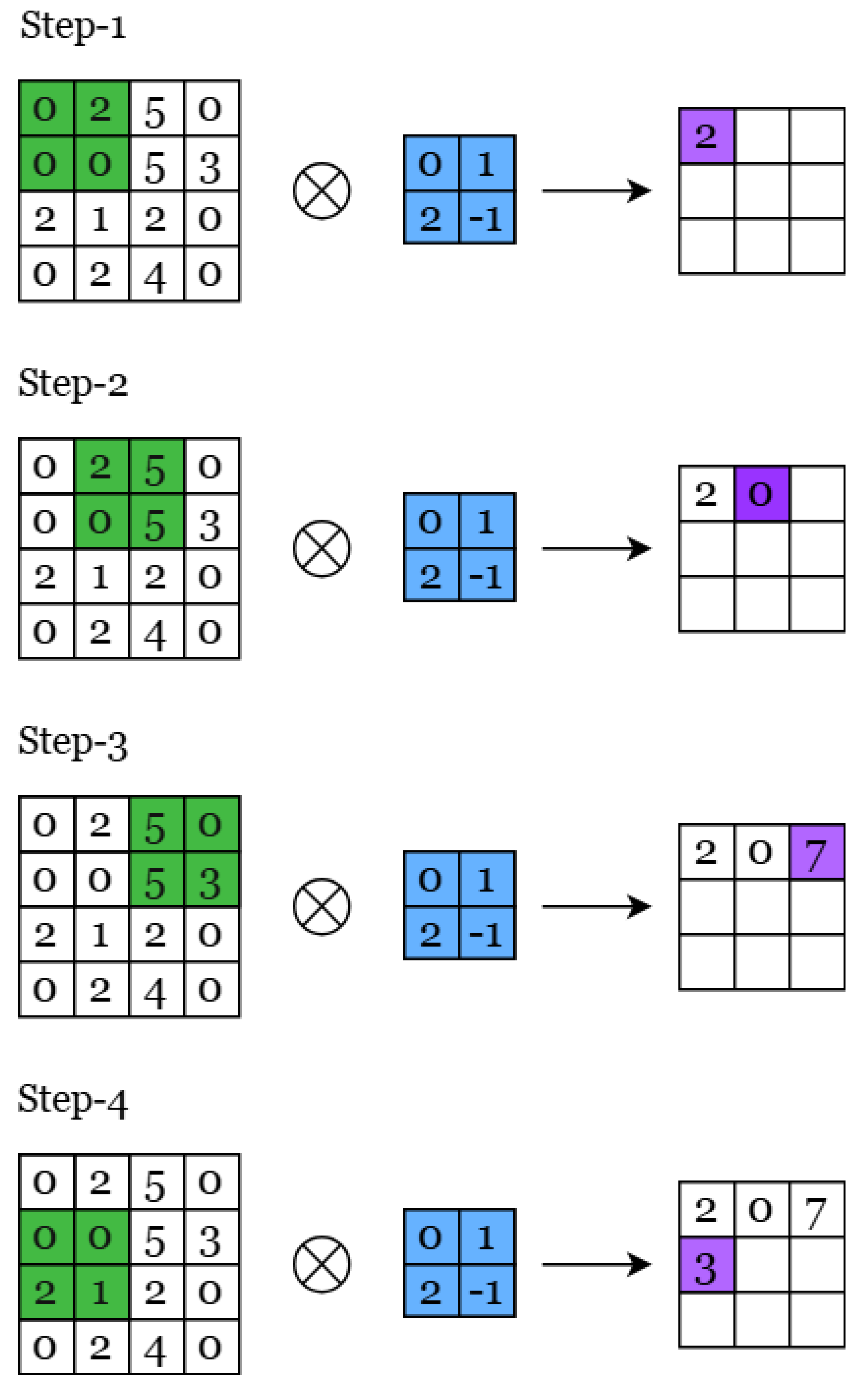
Figure 3.
Visual comparison between hierarchical processing in the mammalian brain and feature extraction in CNNs. Low-level regions extract edges, lines and dark spots; mid-level regions extract parts like eyes/nose; high-level regions respond to complete faces and categories.
Figure 3.
Visual comparison between hierarchical processing in the mammalian brain and feature extraction in CNNs. Low-level regions extract edges, lines and dark spots; mid-level regions extract parts like eyes/nose; high-level regions respond to complete faces and categories.
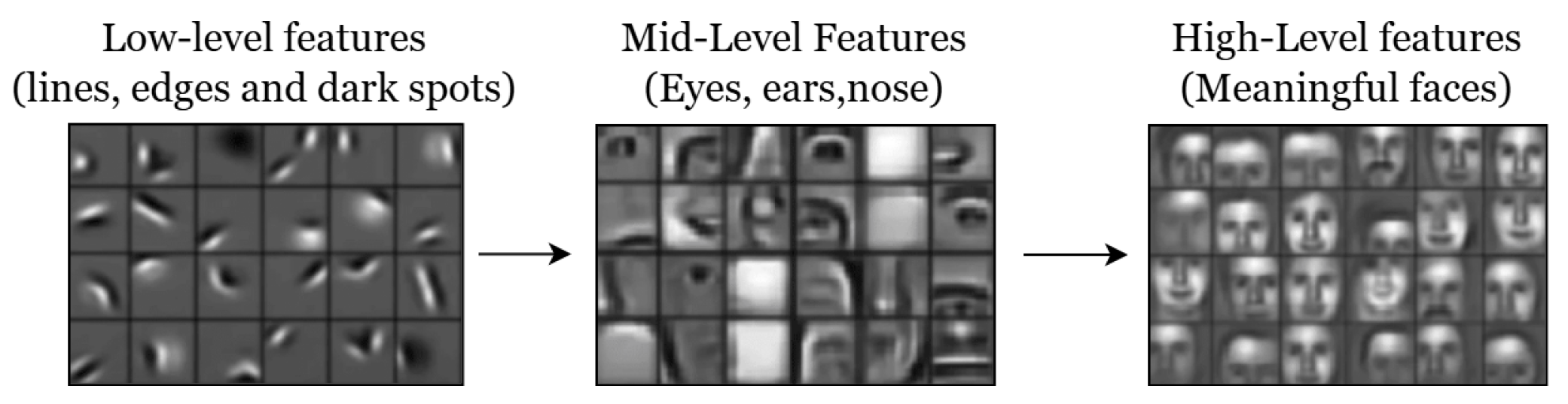
Disclaimer/Publisher’s Note: The statements, opinions and data contained in all publications are solely those of the individual author(s) and contributor(s) and not of MDPI and/or the editor(s). MDPI and/or the editor(s) disclaim responsibility for any injury to people or property resulting from any ideas, methods, instructions or products referred to in the content. |
© 2025 by the authors. Licensee MDPI, Basel, Switzerland. This article is an open access article distributed under the terms and conditions of the Creative Commons Attribution (CC BY) license (http://creativecommons.org/licenses/by/4.0/).
Copyright: This open access article is published under a Creative Commons CC BY 4.0 license, which permit the free download, distribution, and reuse, provided that the author and preprint are cited in any reuse.


