Submitted:
13 October 2025
Posted:
14 October 2025
You are already at the latest version
Abstract
The purpose of infrared and visible image fusion is to integrate their complementary information into a single image, thereby increasing the amount of information expression. However, previous methods often struggle to extract information hidden in darkness, and existing methods, which integrate brightness enhancement and image fusion, can cause overexposure, image blocking effects, and color deviation. Therefore, we propose a visible light and infrared image fusion method, CDFFusion, for low-light scenarios. Specifically, our method consists of two stages: First, an encoder is designed to extract deep features of visible light and infrared images respectively. Then, combined with RetiNex theory, a decomposition network is designed at the feature level to separate the illuminance component and reflectance component of the visible light image. Next, the proposed formula is used to process the Cb and Cr components of the original visible light image. The features of the reflectance component and infrared features are concatenated and input into the fusion network to obtain the Y component of the fused image. Finally, it is concatenated with the processed Cb' and Cr' components of the visible light image to get the final fused image. Experimental results show that the proposed method can effectively alleviate overexposure and image blocking effects, and there is no color deviation at all.
Keywords:
night scene
; image enhancement
; image fusion
1. Introduction
Visible images usually contain rich texture detail information, but they are prone to loss of target information in complex scenes; infrared images, which are formed based on thermal radiation information, are not easily affected by harsh conditions, but they lack detailed descriptions of the scene. Therefore, infrared and visible image fusion (IVIF) can make full use of their complementary information and significantly improve the comprehensive perception ability of the scene. However, in current low-light environments with low visibility, most of the texture details in visible light images are obscured. The general approach to address this issue is to first preprocess the visible light image using a low-light enhancement method and then fuse it with the infrared image. However, this can cause color distortion in some areas, so how to organically combine low-light image enhancement with IVIF is a significant challenge.
Figure 1 shows the visible image, infrared image, the result processed by RFN-Net, and the result processed by LEDNet [1] preprocessing followed by RFN-Net. Firstly, previous IVIF methods fail to extract the information of visible images obscured at night (as shown in the red box in (c)). In contrast, fusing the visible image after enhancement preprocessing causes color distortion in some areas (as shown in the green box in (d), where white zebra crossings are rendered green).
Secondly, existing nighttime IVIF methods, while solving the above two problems, introduce new issues. Figure 2 displays the visible image, infrared image, and the results processed by DIVFusion, LEFuse, LENFusion, and the proposed method. It can be observed that DIVFusion and LEFuse overemphasize the difference between high and low gray values and focus on highlighting high-gray-value regions, which leads to two consequences: first, overexposure occurs in certain parts of the image (the lower left corners in (c) and (d)); second, severe block artifacts (mosaic effect, as shown in the red boxes in (c) and (d)) or false edges appear in non-edge or weak-edge regions. Although LENFusion avoids overexposure, it differs from the previous two methods by focusing on suppressing low-gray-value regions, which also results in two problems: in some weak-edge regions, the low-gray-value parts are severely distorted, leading to information loss (as shown in the red box in (e)); in other weak-edge regions, the colors of these low-gray-value parts are rendered extremely dark, causing unnatural false edges (not shown in the figure). Additionally, these methods only process the Y channel of visible images without handling the Cb and Cr channels, which changes the hue and saturation of the source images, resulting in varying degrees of color deviation.
To solve the above problems, this paper proposes a two-stage network for joint low-light image enhancement and image fusion without color deviation. It can alleviate overexposure and block artifacts while eliminating color deviation. Firstly, an encoder with a Feature Pyramid Network (FPN) structure is used to extract deep features of visible and infrared images respectively. Then, combined with the RetiNex theory, a decomposition network is designed at the feature level to separate the illumination component and reflectance component of the visible image. Next, the proposed formula is applied to process the Cb and Cr components of the original visible image. The reflectance component features and infrared features are concatenated and input into the fusion network to obtain the Y component of the fused image. Finally, the Y component is concatenated with the processed Cb’ and Cr’ components of the visible image to generate the final fused image.
In summary, the main contributions of this paper are as follows:
- This paper proposes a two-stage network for joint low-light image enhancement and image fusion, which can alleviate overexposure and block artifacts while eliminating color deviation, named CDFFusion;
- A brightness enhancement formula without color deviation is proposed, which processes the three components (Y, Cb, Cr) simultaneously, and the processed results have no color deviation;
2. Related Work
Deep learning-based visible and infrared image fusion methods can be roughly divided into three categories: those based on Convolutional Neural Networks (CNN), those based on Autoencoders (AE), and those based on Generative Adversarial Networks (GAN). Zhang et al. proposed a Squeeze-and-Decomposition Network, SD-Net [2], which models image fusion as the extraction and reconstruction of gradient and intensity information. Based on the fact that different fusion tasks share a similar goal—fusing images by integrating important and complementary information from multiple source images—Xu et al. proposed a unified unsupervised end-to-end image fusion network, U2Fusion [3], which is characterized by its ability to perform information measurement on extracted features to automatically estimate the importance of source images. Li et al. proposed an end-to-end fusion network architecture, RFN-Nest [4], which includes an encoder, a Residual Fusion Network (RFN), and a decoder. The encoder extracts multi-scale deep features through max-pooling; the RFN is composed of several convolutional layers and is trained with a new loss function to implement a learnable fusion strategy instead of manually designed rules; the decoder adopts an architecture based on nested connections to reconstruct the fused image. Xu et al. proposed a classification saliency-based pixel-level fusion method, CSF [5], which classifies different source images, uses the classification results to represent the saliency of each pixel in the source images, and finally fuses the feature maps using this saliency to generate the fusion result. Ma et al. first proposed an end-to-end model based on Generative Adversarial Networks (GAN) and named it FusionGAN [6]. It formulates the fusion problem as an adversarial problem while avoiding the manual design of complex activity level measurement and fusion rules. Later, the team designed another Generative Adversarial Network with Multiclassification Constraints, GANMcC [7], which formulates the fusion problem as the simultaneous estimation of multiple distributions.
DIVFusion [8] was the first to combine IVIF and low-light enhancement. It decomposes the visible image into reflectance features and illumination features at the feature level, then enhances and fuses the reflectance features with infrared features. LENFusion [9] adopts the idea of pre-enhancement, re-enhancement, and fusion. It draws on the idea of PIAFusion [10] by pre-training a binary classifier and using its classification results as part of the loss function of the backbone network. LEFuse [11] introduces a hybrid module of Transformer and CNN and designs the overall network structure into a symmetric structure similar to the U-net style.
3. Methods
The proposed method in this paper improves nighttime visibility, retains the complementary information of the two modalities, alleviates overexposure and block artifacts, and eliminates color deviation. This section details the two sub-networks of the entire framework, including the network structure and loss function.
3.1. Overall Framework
All As shown in Figure 3, let and represent the Y channel of the visible image and the infrared image respectively. After passing through the decomposition network and fusion network, the Y channel of the fused image is obtained. Then, it is concatenated with the processed Cb and Cr channels of the visible image to get the final fusion result. The entire process is divided into two stages: feature extraction and image fusion.
3.2. Reflectance-Illumination Decomposition Network(RID-Net)
The specific structure of the reflectance-illumination decomposition network is shown in Figure 4, which consists of two parts: a visible image reconstruction network and an infrared image reconstruction network. The former is used to separate the reflectance and illumination components of the visible image at the feature level and reconstruct them into images, while the latter is used to extract deep features of the infrared image and reconstruct them into images. First, in the feature extraction stage, the Y channel of the visible image is input into the encoder with an FPN structure to extract deep features . The specific structure of the encoder is shown in Figure 5. The original image passes through 4 convolutional layers (C1-C4) in sequence to obtain 4 feature maps of different sizes. The parameters of C1-C4 are listed in Table 1. Then, 4 1×1 convolutional layers (C5-C8) are used to unify the number of channels of the feature maps obtained just now, which is set to 256 here. After that, these processed feature maps are upsampled by 2 times and summed to complete multi-scale fusion. This process can be expressed as:
In the feature separation stage, according to the RetiNex theory, an image can be decomposed into the product of the reflectance component (R) and the illumination component (L) (as shown in the following formula). Therefore, two Efficient Channel Attention (ECA) modules are used to separate the reflectance features and illumination features from them.
The structure of the ECA module is shown in Figure 6. First, global average pooling is performed on each channel of the input feature map to obtain the global feature of each channel. Then, one-dimensional convolution and activation are applied to these global features to obtain attention weights. The input feature map is reweighted using these weights to get the output feature. Here, GAP and represent global average pooling and sigmoid activation function respectively. This process can be expressed as:
In the final decoding stage, they are input into two decoders with identical structures, and the reflectance component and illumination component are obtained through reconstruction. Both decoders are composed of 4 stacked groups of convolutional and activation layers. The first 3 activation layers use the LRelu function, and the last one uses the sigmoid function. This process can be expressed as:
It should be noted that the decoding part here is only for better image reconstruction and does not participate in the operation of the next stage.
Similarly, the infrared reconstruction network adopts a basically consistent structure, which will not be elaborated here.
The loss function of this part of the network is as follows:
The loss function of the visible image reconstruction network consists of two parts: reconstruction loss and perceptual loss . The reconstruction loss is derived from Formula (2), which is expressed as follows:
On this basis, we hope that the brightness-enhanced result (i.e., the reflectance component ) and the result of the original image after histogram equalization have as similar representations as possible in the feature domain of the VGG-19 network. Thus, the perceptual loss is defined as:
where “hist” represents the histogram equalization operation. Here, the Conv4-1 feature of the VGG-19 network is selected.
The loss function of the infrared reconstruction network consists of reconstruction loss and structural similarity loss , which can reconstruct results similar to the original image in both intensity and structure. It is defined as follows:
Here, are weight hyperparameters used to balance the various parts of the loss.
3.3. Fusion Network
In the fusion stage, the reflectance features of the visible image and the infrared features are concatenated at the channel level and input into the fusion network. Consistent with the decoder structure in the previous stage, it is also composed of 4 stacked groups of convolutional and activation layers. At this time, its output is taken as the Y channel of the fused image, which is used to participate in the final channel fusion.
According to the ITU-R BT.601 international standard, the conversion formula from the RGB space to the YCbCr space of an image is:
In the HSI color space, the conversion formula from RGB to HSI is:
where H represents hue and S represents saturation. From the above formula, it can be proved that: only when the three components R, G, and B are scaled proportionally, the hue and saturation of the pixel remain unchanged. Substituting the result into Formula (9), it can be obtained that: only when (Cb - 0.5) and (Cr - 0.5) are scaled synchronously with Y, R, G, and B are scaled proportionally (the pixel value range has been normalized to [0, 1]), and the hue and saturation remain unchanged. Thus, we naturally derive the mapping formula for the Cb and Cr channels of the visible image:
where “scale” is the brightness gain image. Different from other methods that use loss functions for weak constraints, the above formula applies strong constraints on the proportion between the three components R, G, and B of the visible image, thus avoiding color distortion. Finally, is concatenated with and , and converted back to the RGB space to obtain the final fused image .
The loss function of the fusion network is as follows:
It consists of visible light intensity loss , infrared intensity loss , auxiliary intensity loss , gradient loss , and structural similarity loss , which are defined as follows:
where represents the gradient operation, and the Sobel operator is used here. These losses can force the fused image to retain more prominent intensity and gradient information from the source images and maintain a relatively consistent structural similarity with the source images. Here, are weight hyperparameters used to balance the various parts of the loss.
4. Experiments
4.1. Experimental Configuration
To comprehensively evaluate the proposed method, extensive experiments are conducted on the LLVIP dataset [12]. The LLVIP dataset is a paired visible-infrared dataset for low-light scenarios, containing 33,672 images (16,836 pairs). Among them, 240 pairs of infrared and visible images are selected for the training phase, and 50 pairs are selected for the testing phase. These images have been strictly registered. The results of this paper are compared with 5 fusion methods, including 1 AE-based method (RFN-Nest), 1 GAN-based method (FusionGAN), and three latest nighttime IVIF methods (DIVFusion, LEFuse, and LENFusion). The implementation of all methods is based on publicly available code.
In the quantitative evaluation phase, six metrics are used, including 1 image feature-based metric (Spatial Frequency, SF), 1 structural similarity-based metric (Multi-Scale Structural Similarity, MS-SSIM), and 4 metrics based on the source images and generated images (Correlation Coefficient, CC; Sum of Correlation Differences, SCD; Gradient-Based Fusion Performance, Qabf; and Noise-Based Fusion Performance, Nabf). Among them, a smaller Nabf value indicates a better fusion effect.
In the training phase, the 240 pairs of images used for training are randomly cropped to a size of 224×224 pixels, and the batch size is set to 5. The initial learning rates of the visible and infrared images in the decomposition network are 10^-4 and 10^-3 respectively, and they are decayed to 0.1 and 0.01 of the initial values after 50 and 75 epochs. The fusion network uses a fixed learning rate set to 2×10^-5. In addition, the weight hyperparameters of the loss functions of the decomposition network and fusion network are set as follows:
4.2. Results and Analysis
4.2.1. Qualitative Comparison
Figure 7 shows the visualization results of different fusion methods. As mentioned earlier, previous fusion methods fail to extract the information of visible images obscured at night. In the results of RFN-Nest and FusionGAN, the upper part of the images in the first row is still completely black, with no significant improvement in brightness, and the zebra crossings in the red boxes become blurred, with the zebra crossings in the upper right corner showing a greenish tint. In the second row of images, most details of the road in the boxes are lost, and the headlight area in the lower right corner is covered with a shadow. In the third row of images, the road details are completely lost. For the results of DIVFusion, LEFuse, and LENFusion, the color saturation in figures (e) and (f) is relatively low, leading to an overexposed feeling in some areas (as shown in the green boxes in the second row of images). In figure (g), areas such as zebra crossings are prone to distortion, resulting in information loss (as shown in the red boxes in the first and second rows of images). In areas such as damaged roads, the color is darkened, forming unnatural false edges (as shown in the green box in the first row of images). In addition, these three methods all cause block artifacts (as shown in the boxes in the third row of images). In the third row of images, the color saturation of buildings and leaves is significantly low, with varying degrees of color deviation. In contrast, the proposed method alleviates all the above issues and achieves a better visual effect without color deviation.
4.2.2. Quantitative Comparison
Table 2 shows the average quality metrics of different fusion methods on the LLVIP dataset. It can be seen that the proposed method ranks first in the Qabf and MS-SSIM metrics, second in the CC and SCD metrics, and third in the SF and Nabf metrics. This indicates that the proposed method can suppress block artifacts while maintaining good high-frequency details, and can well maintain the consistency between the fused image and the source images.
4.3. Generalization Experiment
To verify the generalization ability of the proposed model, 48 pairs of images are selected from the M3FD dataset [13] for testing. The model is not trained on the M3FD dataset and is directly used for testing. The M3FD dataset is a visible-infrared fusion dataset, containing 4,200 pairs of images for fusion, detection, and fusion-based detection, as well as 300 pairs of images for independent scene fusion.
4.3.1. Qualitative Comparison
As shown in Figure 8, first, in the result of RFN-Nest, the information on the signs is obscured in darkness and cannot be seen clearly (as shown in the green box in the first row of images and the red box in the second row of images). Secondly, the results of RFN-Nest and FusionGAN are generally blurrier than the original images (such as the tree areas in the first row of images). In the results of DIVFusion, LEFuse, and LENFusion, snowflake-like noise appears in the sky area of the first row of images, and the outline of the clouds is eroded (as shown in the red box in the first row of images). In the second row of images, the outline of distant buildings becomes incomplete compared with the original image. In addition, the results of these three methods all have varying degrees of color distortion, and figure (f) even gives an overexposed feeling.
4.3.2. Quantitative Analysis
Table 3 shows the average quality metrics of different fusion methods on the M3FD dataset. It can be seen that the proposed method ranks first in the Qabf metric, second in the SF and CC metrics, and third in the Nabf, SCD, and MS-SSIM metrics. This indicates that the proposed method can retain rich texture details and well maintain the correlation and consistency between the fused image and the source images.
4.4. Ablation Experiment
To verify the effectiveness of each loss function in the proposed method, an ablation experiment is designed. To verify the effectiveness of the perceptual loss and auxiliary intensity loss , these two loss functions are removed respectively, and the results are shown in Figure 9.
4.4.1. Qualitative Comparison
When the perceptual loss is removed, the fused image exhibits severe color deviation and block artifacts. In fact, at this time, the RID-Net cannot accurately separate the reflectance component . When the auxiliary intensity loss is removed, the fused image fails to express sufficient infrared information (as shown in the green box in Figure (d)), and a lot of road texture information is lost (as shown in the red box in Figure (d)).
4.4.2. Quantitative Analysis
The quantitative results of the ablation experiment are shown in Table 4. It can be seen that the proposed method achieves better results in the CC, Qabf, and SCD metrics. The SF is not the optimal because areas with block artifacts often have higher spatial frequencies. The MS-SSIM is also not the optimal because without the auxiliary intensity loss , the fused image tends to be closer to either the visible image or the infrared image.
5. Conclusions and Discussion
This paper proposes a new fusion method to address the shortcomings of existing visible and infrared image fusion methods in low-light scenarios. CDFFusion adopts a two-stage strategy to solve the problems of overexposure and block artifacts, and completely avoids color deviation. Specifically, we first train a feature extraction network that can extract features of source images and separate the illumination component and reflectance component of the visible image. Then, a fusion network is trained, which combines the proposed color mapping formula to realize fusion of infrared images and enhanced visible images without color deviation. Experimental results show that compared with the existing five methods, the proposed method achieves generally better results in both subjective and objective aspects.
The limitations of this paper are as follows: the encoder with the FPN structure has certain requirements on the size of the input image, requiring both the height and width of the image to be integer multiples of 8. Images that do not meet the size requirements need to be preprocessed. In addition, there are certain shortcomings in the feature extraction of infrared images, and the unique advantages of infrared images are not separated and fully utilized.
Appendix A
Theorem 1.
Condition for Constant H and S.
Two pixels have the same H and S if and only if the three terms (Y, Cb - 0.5, Cr - 0.5)(normalized) of the two pixels are proportional to each other respectively. follows:
Proof of Theorem 1.
Let and .According to Equation (10), we have and , where , , and are non - zero.
Now, consider the following system of equations:
To further simplify , we perform congruent diagonalization on matrix A. Let , then , where . For any arbitrary x, there always exists a unique s such that . Substitute this into the expressions of :
We obtain , where and are not 0 simultaneously. Let , and substitute it into the first equation of the system (15):
We obtain , After simplification, we get , where m is a positive real number and n is any real number.
Substitute and into the above equation, we have or , where .
The following is the discussion by cases:
- 1.
- First item;
In this case, the equation hold, thus the magnitude relationship of is the same as that of . Let ,Then we have: , where .
Denote as the i - th row of any matrix M. Then , (where E is the 3×3 identity matrix), so .
Substitute the above formula into the second equation of the system (15), we get . Substitute the expression of into this equation, and considering that , the equation simplifies to . Further, considering that , the equation finally simplifies to .
Substitute it into the expression of , we obtain .
Substitute it back into the original system (15) for verification, and it holds.
- 2.
- Second item;
Note that , i.e., , so the magnitude relationship of is opposite to that of .
In this case, , and the original system (15) does not hold, so this case is discarded.
To sum up, the system (15) holds if and only if , which means the two pixels have the same H and S.
Now, normalize the pixel values and let and .From Equation (9), we have , where .
Note that matrix B is invertible, so if is to hold, then must hold. □
References
- Shangchen Zhou, Chongyi Li & Chen Change Loy. LEDNet: Joint Low-Light Enhancement and Deblurring in the Dark[C]//Computer Vision – ECCV 2022. 2022.
- Hao Zhang, Jiayi Ma. SDNet: A Versatile Squeeze-and-Decomposition Network for Real-Time Image Fusion[J]. International Journal of Computer Vision, 2021,Vol. 129(10): 2761-2785.
- Han Xu, Jiayi Ma, Junjun Jiang, et al. U2Fusion: A Unified Unsupervised Image Fusion Network[J]. IEEE transactions on pattern analysis and machine intelligence, 2022, Vol.44(1): 502-518.
- Hui Li, Xiao-Jun Wu, Josef Kittler. RFN-Nest: An end-to-end residual fusion network for infrared and visible images[J]. Information Fusion, 2021, Vol.73: 72-86.
- Xu, Han, Zhang, et al. Classification saliency-based rule for visible and infrared image fusion.[J]. IEEE Trans. Comput. Imaging, 2021, Vol.7: 824-836.
- Jiayi Ma, Wei Yu, Pengwei Liang, et al. FusionGAN: A generative adversarial network for infrared and visible image fusion[J]. Information Fusion, 2019, Vol.48: 11-26.
- Jiayi Ma, Hao Zhang, Zhenfeng Shao, et al. GANMcC: A Generative Adversarial Network With Multiclassification Constraints for Infrared and Visible Image Fusion[J]. Instrumentation and Measurement, IEEE Transactions on, 2021,Vol.70: 1-14.
- Linfeng Tang, Xinyu Xiang, Hao Zhang, et al. DIVFusion: Darkness-free infrared and visible image fusion[J]. Information Fusion, 2023, Vol.91: 477-493.
- Jun Chen, Liling Yang, Wei Liu, et al. LENFusion: A Joint Low-Light Enhancement and Fusion Network for Nighttime Infrared and Visible Image Fusion[J]. IEEE Transactions on Instrumentation and Measurement, 2024, Vol.73: 1-15.
- Linfeng Tang, Jiteng Yuan, Hao Zhang, et al. PIAFusion: A progressive infrared and visible image fusion network based on illumination aware[J]. Information Fusion, 2022, Vol.83: 79-92.
- Cheng, MuhangCAa, Huang, et al. LEFuse: Joint low-light enhancement and image fusion for nighttime infrared and visible images[J]. Neurocomputing, 2025, Vol.626: 129592.
- Jia, Xinyu, Zhu, et al. LLVIP: A Visible-infrared Paired Dataset for Low-light Vision[C]//18th IEEE/CVF International Conference on Computer Vision Workshops, ICCVW 2021. 2021.
- Liu, Jinyuan, Fan, et al. Target-aware Dual Adversarial Learning and a Multi-scenario Multi-Modality Benchmark to Fuse Infrared and Visible for Object Detection[C]//2022 IEEE/CVF Conference on Computer Vision and Pattern Recognition (CVPR). 2022.
- MA J Y, TANG L F, XU M L, et al. STDFusionNet: an infrared and visible image fusion network based on salient target detection[J]. IEEE Transactions on Instrumentation and Measurement, 2021, 70: 1-13.
- Liu Y, Chen X, Ward R K, et al. Image fusion with convolutional sparse representation[J]. IEEE signal processing letters, 2016, 23(12): 1882-1886.
- LI H, WU X J, KITTLER J. Infrared and visible image fusion using a deep learning framework[C]// 2018 24th International Conference on Pattern Recognition(ICPR). 2018:2705-2710.
- LI H, WU X J, DURRANI T S. Infrared and visible image fusion with ResNet and zero-phase component analysis[J].Infrared Physics & Technology, 2019, 102:103039.
- LI H, WU X J. DenseFuse: a fusion approach to infrared and visible images[J]. IEEE Transactions on Image Processing, 2019, 28(5): 2614-2623.
- XU H, GONG M Q, TIAN X, et al. CUFD: an encoderdecoder network for visible and infrared image fusion based on common and unique feature decomposition[J]. Computer Vision and Image Understanding, 2022, 218: 103407.
- XU H, LIANG P W, YU W, et al. Learning a generative model for fusing infrared and visible images via conditional generative adversarial network with dual discriminators[C]// Proceedings of the 28th International Joint Conference on Artificial Intelligence, Macao, China, Aug 10-16, 2019: 3954-3960.
Figure 1.
Fusion results of previous methods on the LLVIP dataset.
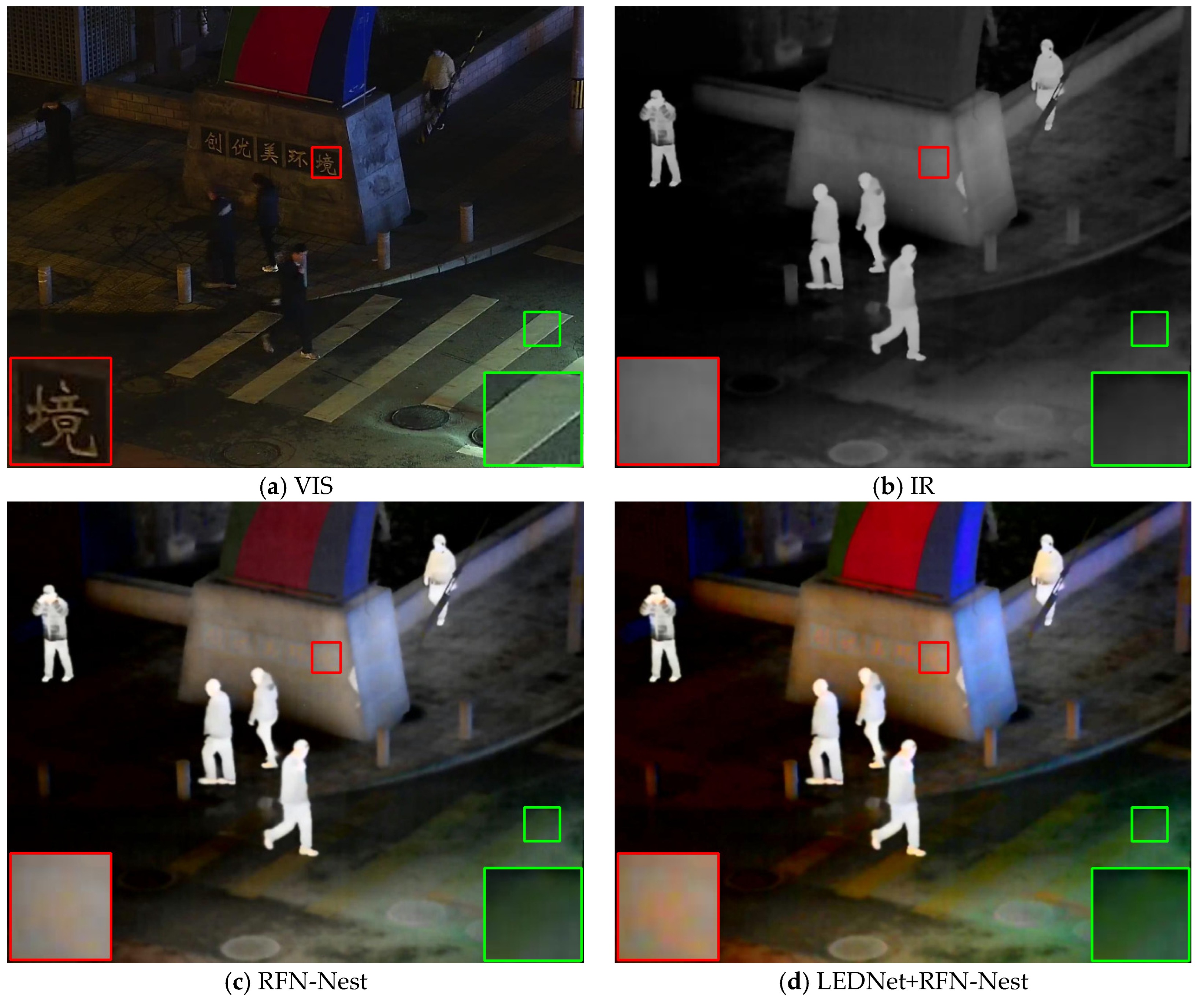
Figure 2.
Fusion results of some recent methods and the proposed method on the LLVIP dataset.
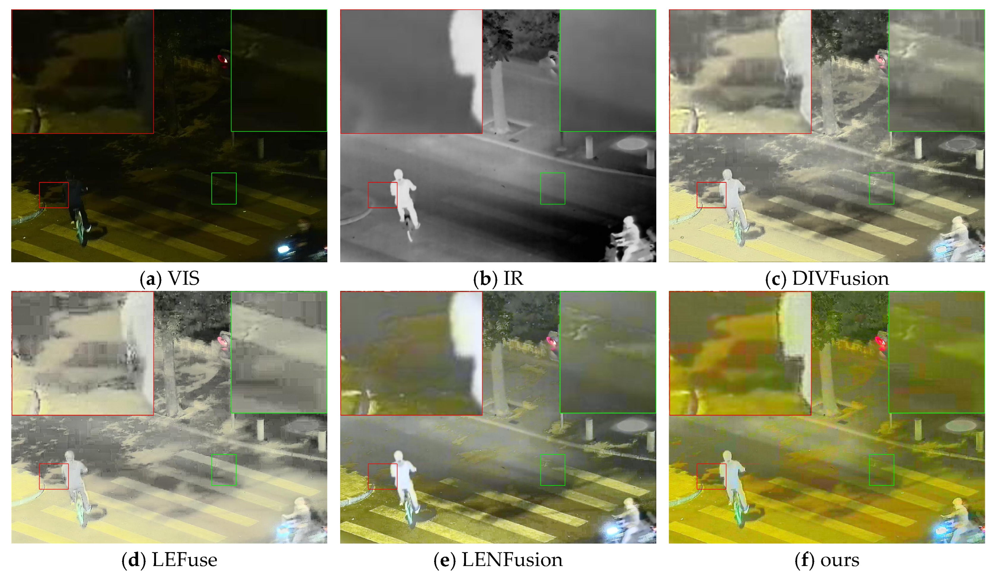
Figure 3.
This Overall framework of CDFFusion.
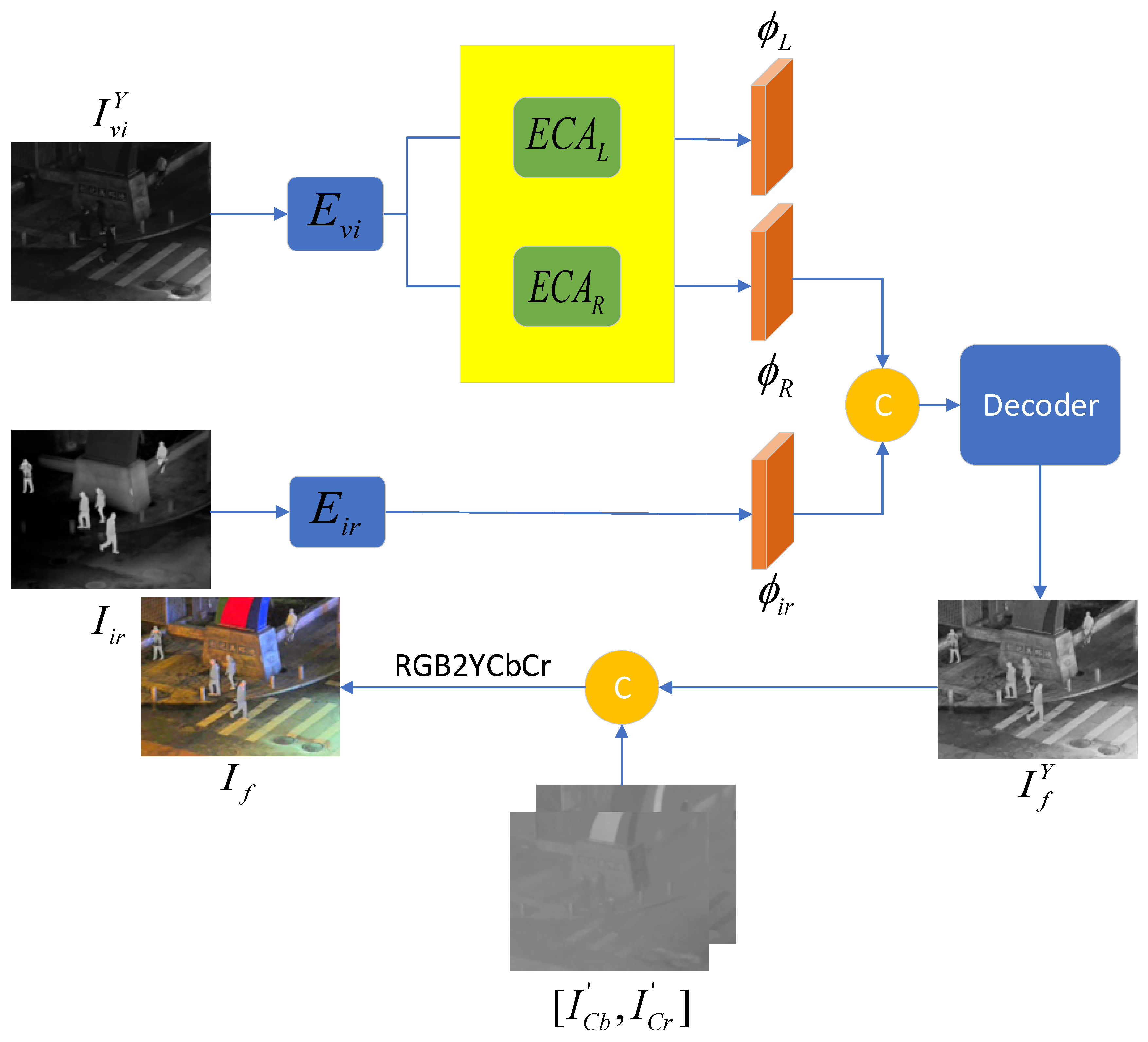
Figure 4.
Structure of the RID-Net.
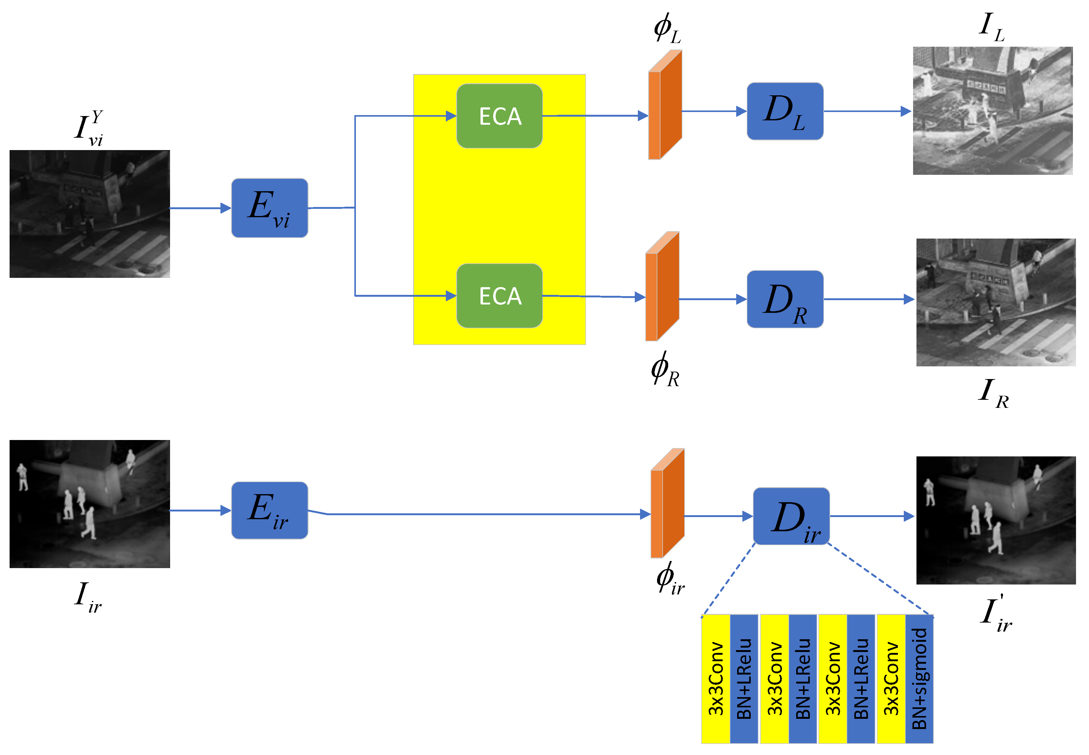
Figure 5.
Structure of the encoder.
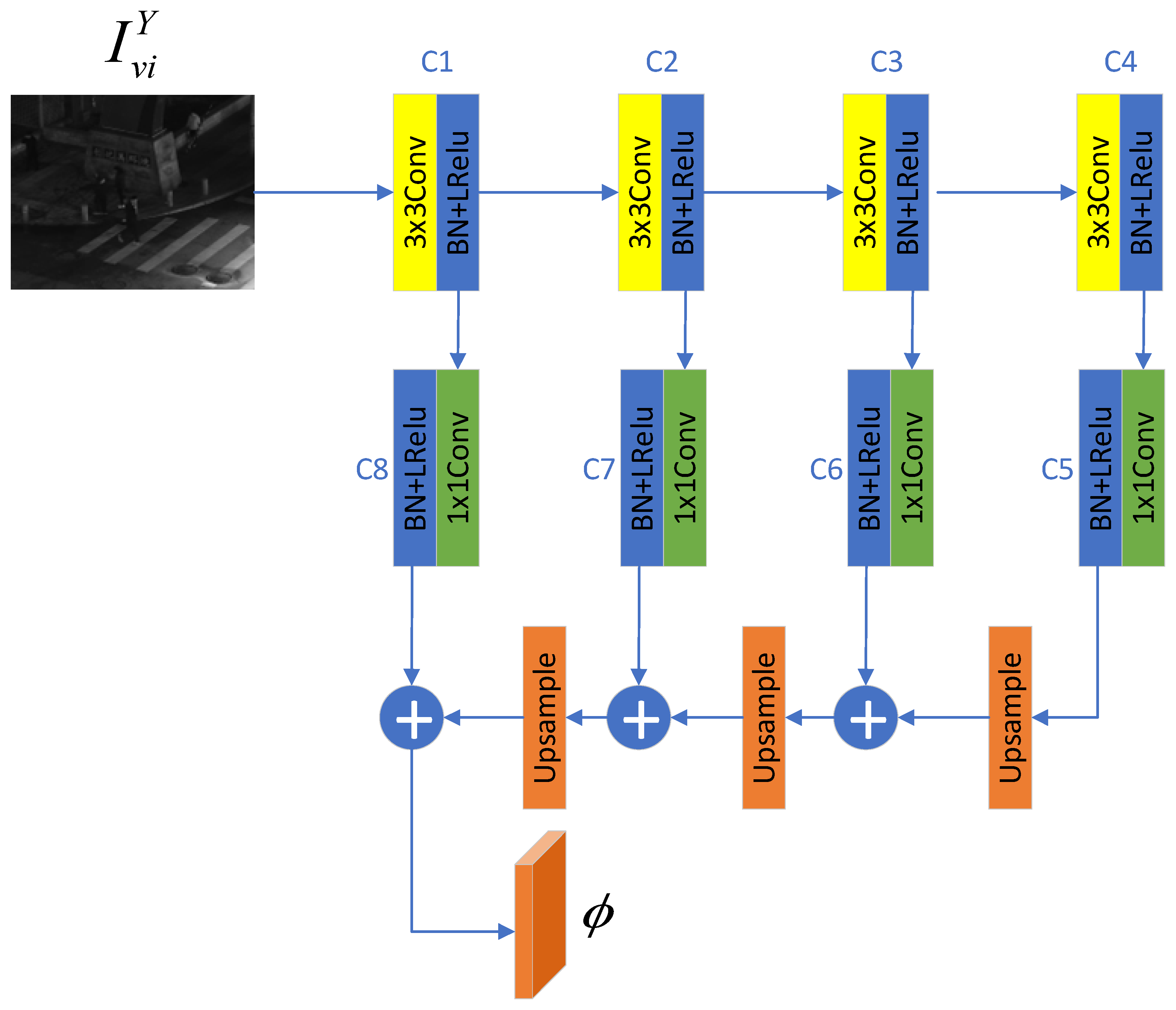
Figure 6.
Structure of the ECA module.
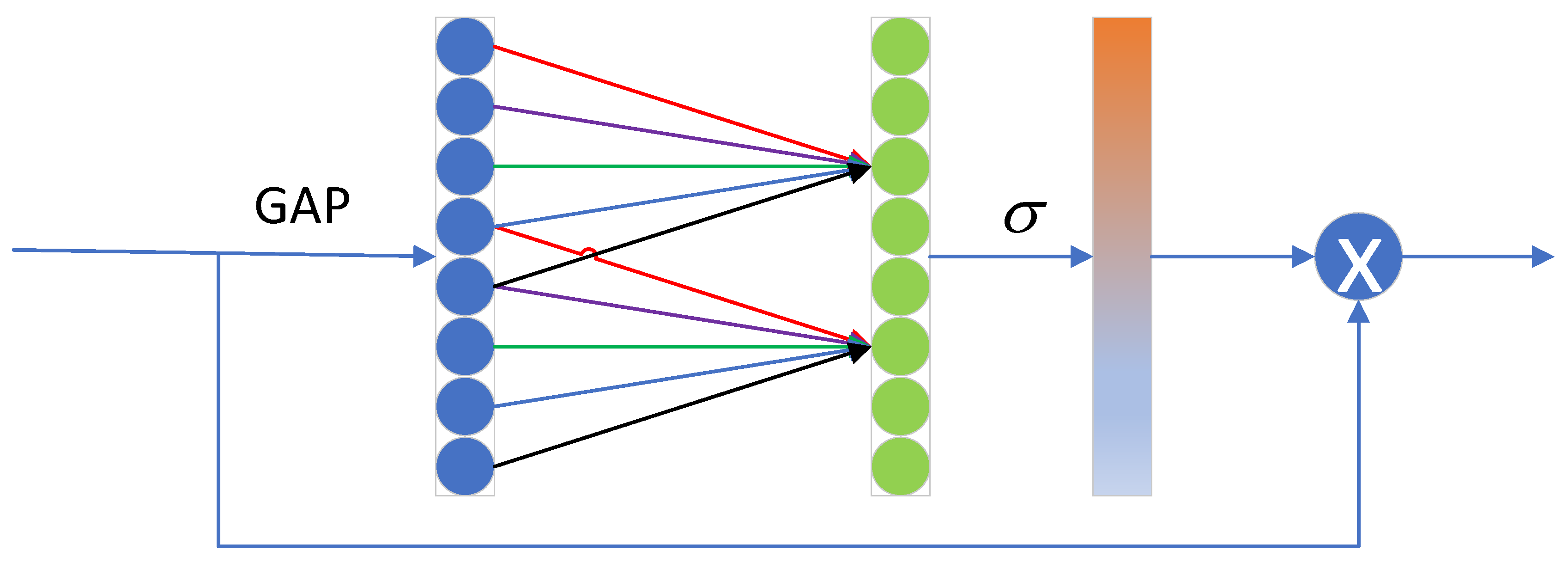
Figure 7.
Experimental results of different methods on the LLVIP dataset.
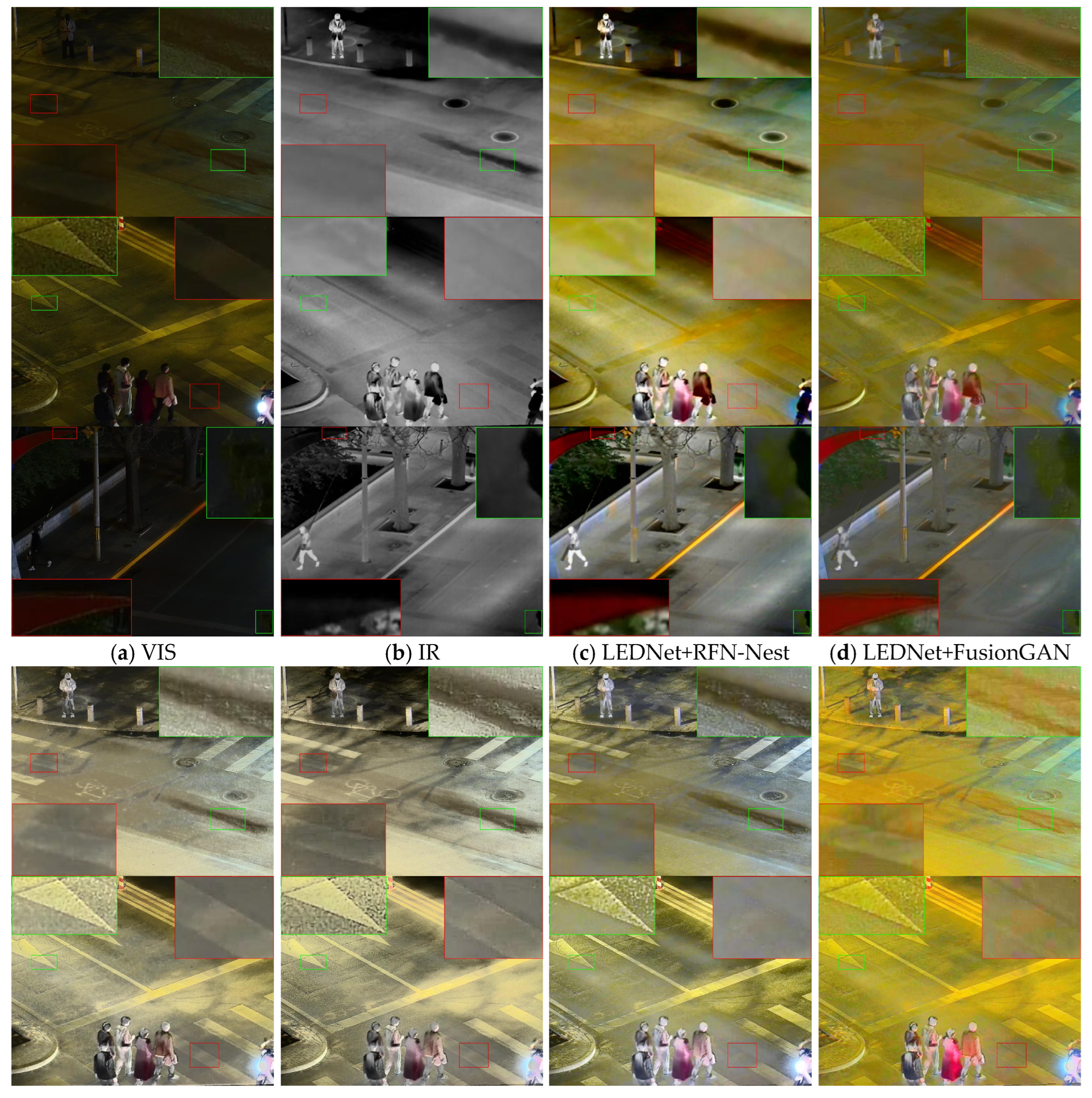
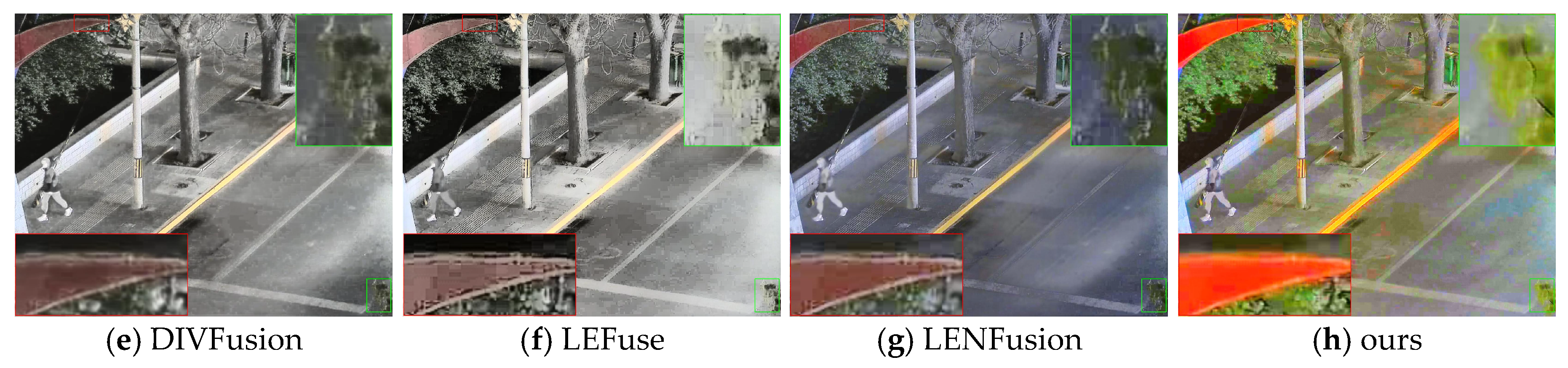
Figure 8.
Experimental results of different methods on the M3FD dataset.
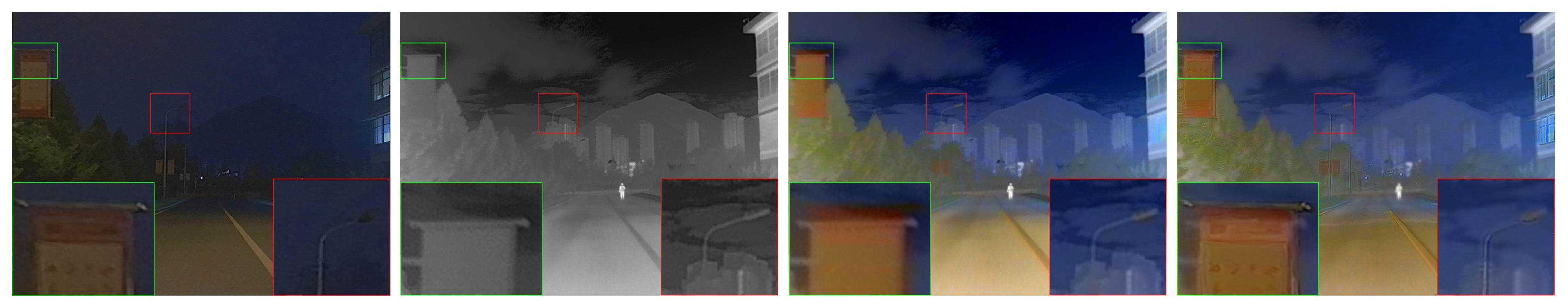
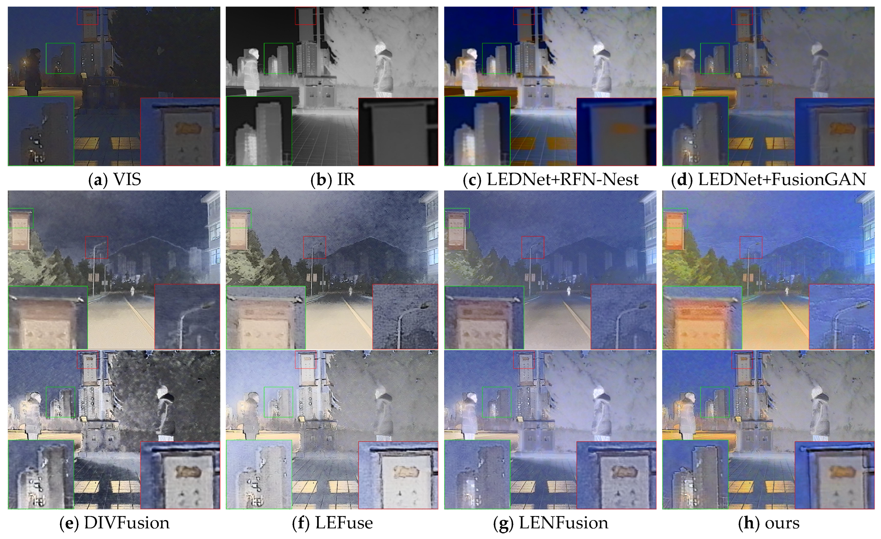
Figure 9.
Comparison of results of the ablation experiment on perceptual loss and auxiliary intensity loss based on the LLVIP dataset.
Figure 9.
Comparison of results of the ablation experiment on perceptual loss and auxiliary intensity loss based on the LLVIP dataset.
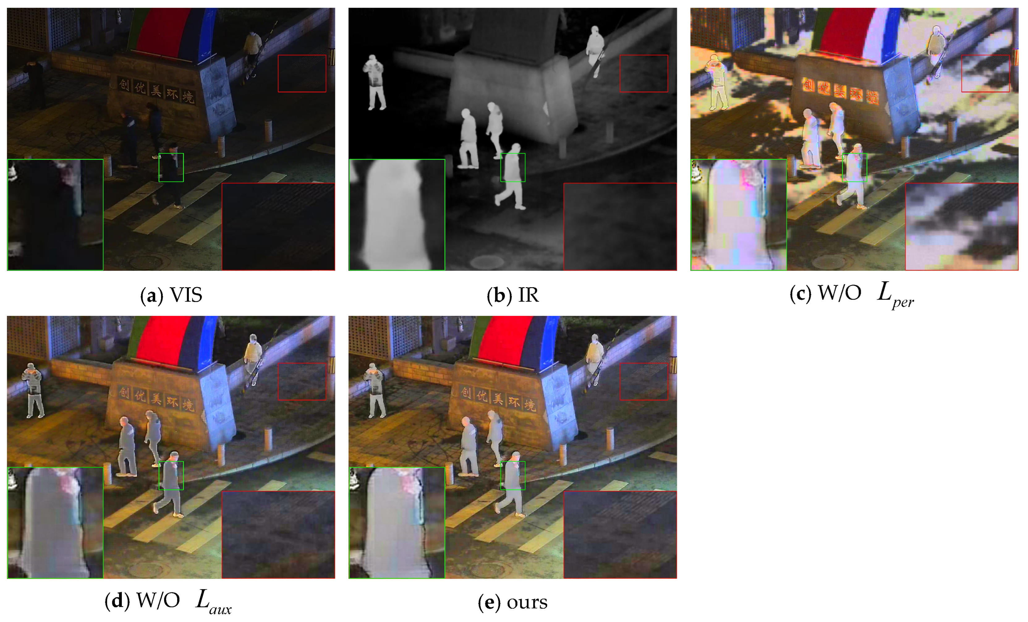

Table 1.
Parameters of C1-C4.
| In channels | Out channels | Kernel size | stride | padding | |
|---|---|---|---|---|---|
| C1 | 1 | 64 | 3 | 1 | 1 |
| C2 | 64 | 128 | 3 | 2 | 1 |
| C3 | 128 | 256 | 3 | 2 | 1 |
| C4 | 256 | 512 | 3 | 2 | 1 |
Table 2.
Quantitative comparison between the proposed method and other methods on the LLVIP dataset. The best and second-best results are marked in bold and underlined respectively.
Table 2.
Quantitative comparison between the proposed method and other methods on the LLVIP dataset. The best and second-best results are marked in bold and underlined respectively.
| SF | CC | Nabf | Qabf | SCD | MS-SSIM | |
|---|---|---|---|---|---|---|
| RFN-Nest | 5.0344 | 0.5824 | 0.0099 | 0.3332 | 1.0923 | 0.7730 |
| FusionGAN | 6.7466 | 0.6479 | 0.0124 | 0.2788 | 0.9159 | 0.8188 |
| DIVFusion | 14.7371 | 0.6922 | 0.1364 | 0.3823 | 1.5373 | 0.7973 |
| LEFuse | 24.0328 | 0.6087 | 0.1856 | 0.3006 | 1.2262 | 0.7027 |
| LENFusion | 21.4990 | 0.5928 | 0.1969 | 0.3534 | 1.0440 | 0.7236 |
| ours | 17.6531 | 0.6619 | 0.1075 | 0.4279 | 1.2760 | 0.8335 |
Table 3.
Quantitative comparison between the proposed method and other methods on the M3FD dataset. The best and second-best results are marked in bold and underlined respectively.
Table 3.
Quantitative comparison between the proposed method and other methods on the M3FD dataset. The best and second-best results are marked in bold and underlined respectively.
| SF | CC | Nabf | Qabf | SCD | MS-SSIM | |
|---|---|---|---|---|---|---|
| RFN-Nest | 4.1495 | 0.6260 | 0.0039 | 0.3133 | 0.9690 | 0.8565 |
| FusionGAN | 6.2380 | 0.6579 | 0.0143 | 0.2770 | 0.7082 | 0.8788 |
| DIVFusion | 14.4927 | 0.7360 | 0.1525 | 0.3684 | 1.6140 | 0.8276 |
| LEFuse | 20.6205 | 0.6623 | 0.2416 | 0.2504 | 1.2501 | 0.7236 |
| LENFusion | 14.6193 | 0.6640 | 0.1402 | 0.3637 | 0.9860 | 0.8011 |
| ours | 16.4501 | 0.6879 | 0.1251 | 0.3694 | 1.0070 | 0.8416 |
Table 4.
Results of the ablation experiment based on the LLVIP dataset. The best results are marked in bold.
Table 4.
Results of the ablation experiment based on the LLVIP dataset. The best results are marked in bold.
| SF | CC | Nabf | Qabf | SCD | MS-SSIM | |
|---|---|---|---|---|---|---|
| W/O | 17.7592 | 0.209 | 0.0868 | 0.4103 | 0.1861 | 0.6925 |
| W/O | 15.3465 | 0.6607 | 0.0957 | 0.4169 | 1.242 | 0.8699 |
| ours | 17.6531 | 0.6619 | 0.1075 | 0.4279 | 1.276 | 0.8335 |
Disclaimer/Publisher’s Note: The statements, opinions and data contained in all publications are solely those of the individual author(s) and contributor(s) and not of MDPI and/or the editor(s). MDPI and/or the editor(s) disclaim responsibility for any injury to people or property resulting from any ideas, methods, instructions or products referred to in the content. |
© 2025 by the authors. Licensee MDPI, Basel, Switzerland. This article is an open access article distributed under the terms and conditions of the Creative Commons Attribution (CC BY) license (https://creativecommons.org/licenses/by/4.0/).
Copyright: This open access article is published under a Creative Commons CC BY 4.0 license, which permit the free download, distribution, and reuse, provided that the author and preprint are cited in any reuse.


