A Geometric Approach to Understanding the Riemann Hypothesis: Exploring Connections Between Geometric Sequences and Zeta Function Zeros

1. Introduction

The Riemann Hypothesis, formulated by Bernhard Riemann in 1859, remains one of the most significant unsolved problems in mathematics. It concerns the distribution of the non-trivial zeros of the Riemann zeta function and has profound implications for our understanding of prime numbers and their distribution.

1.1. The Riemann Zeta Function and Its Zeros

The Riemann zeta function is defined for complex numbers $s=\sigma +it$ with $\sigma >1$ by the absolutely convergent series:

$$\zeta \left(s\right)=\sum _{n=1}^{\infty }{\displaystyle \frac{1}{n^s}}=\prod _{p\mathrm{prime}}{\displaystyle \frac{1}{1-p^{-s}}}$$

(1)

Through analytic continuation, $\zeta \left(s\right)$ extends to a meromorphic function on the entire complex plane, with a simple pole at $s=1$. The function has trivial zeros at $s=-2,-4,-6,\dots$ and infinitely many non-trivial zeros in the critical strip $0<\mathrm{Re}\left(s\right)<1$.

Conjecture 1

(Riemann Hypothesis). All non-trivial zeros of the Riemann zeta function have real part equal to ${\displaystyle \frac{1}{2}}$.

1.2. Motivation for a Geometric Approach

Traditional approaches to the Riemann Hypothesis have primarily relied on complex analysis, harmonic analysis, and number theory. In this paper, we explore a different perspective by introducing geometric constructions that may shed new light on the problem.

Our approach is motivated by the observation that many deep results in mathematics emerge from the interplay between different mathematical domains. By translating the analytical properties of the zeta function into geometric language, we hope to gain new insights into its structure.

1.3. Overview of Our Approach

We construct a geometric sequence based on a recurrence relation that incorporates:

• A parameter a that corresponds to the real part of zeta function zeros
• Trigonometric terms that encode information about the imaginary parts
• A geometric interpretation through triangular constructions and the cosine law

The central question we investigate is: under what conditions does this geometric sequence converge, and how do these conditions relate to the Riemann Hypothesis?

2. Geometric Construction and Mathematical Framework

2.1. The Fundamental Recurrence Relation

2.1.1. Mathematical Motivation

Our approach is motivated by the desire to construct a geometric sequence whose convergence properties mirror those of the Dirichlet eta function, which is closely related to the Riemann zeta function. We seek a recurrence relation that:

1.

Incorporates the parameter structure of zeta function zeros

2.

Has a natural geometric interpretation

3.

Exhibits convergence behavior linked to the critical line

2.1.2. Derivation of the Recurrence Relation

Consider the Dirichlet eta function:

$$\eta \left(s\right)=\sum _{n=1}^{\infty }{\displaystyle \frac{{(-1)}^{n+1}}{n^s}}=(1-2^{1-s})\zeta \left(s\right)$$

(2)

For $s=a+it$ with $a>0$, we can write:

$$\eta (a+it)=\sum _{n=1}^{\infty }{\displaystyle \frac{{(-1)}^{n+1}}{n^a}}{e}^{-itlnn}$$

(3)

To construct a geometric analogue, we define a sequence ${\left\{F\left(n\right)\right\}}_{n=0}^{\infty }$ that mimics the partial sums of a related series. The key insight is to relate the squared differences $F^2\left(n\right)-F^2(n-1)$ to the geometric construction.

Theorem 2

(Fundamental Recurrence Relation). The sequence ${\left\{F\left(n\right)\right\}}_{n=0}^{\infty }$ is defined by the recurrence relation:

$$F^2\left(n\right)-F^2(n-1)=2F(n-1){(n+1)}^{-a}cos\left(tln{\displaystyle \frac{n}{n-1}}\right)+{(n+1)}^{-2a}$$

(4)

for $n\ge 1$, with initial condition $F\left(0\right)=1$, where:

• $a\in (0,1)$ is a parameter corresponding to the real part of a zeta function zero
• $t\in \mathbb{R}$ represents the imaginary part of a potential zero
• The logarithmic term $ln{\displaystyle \frac{n}{n-1}}$ encodes the discrete derivative structure

Derivation. 

The recurrence relation is constructed to satisfy the following properties:

1. Asymptotic behavior: For large n, we have $ln{\displaystyle \frac{n}{n-1}}\approx {\displaystyle \frac{1}{n}}$, so the cosine term becomes $cos\left({\displaystyle \frac{t}{n}}\right)\approx 1-{\displaystyle \frac{t^2}{2n^2}}$.

2. Geometric interpretation: The term ${(n+1)}^{-2a}$ represents the squared distance between consecutive points in our geometric construction.

3. Oscillatory behavior: The cosine term introduces oscillations that mirror the behavior of the zeta function on the critical line.

The specific form ensures that the sequence has the desired convergence properties when $a={\displaystyle \frac{1}{2}}$. □

2.1.3. Properties of the Recurrence Relation

Lemma 1

(Positivity and Boundedness). If $F\left(0\right)=1$ and $a>0$, then:

1.

$F\left(n\right)\ge 0$ for all $n\ge 0$

2.

The sequence $\left\{F\right(n\left)\right\}$ is bounded if $a>{\displaystyle \frac{1}{2}}$

Proof. 

The positivity follows from the fact that $F^2\left(n\right)\ge 0$ by definition. For boundedness, we note that when $a>{\displaystyle \frac{1}{2}}$, the terms ${(n+1)}^{-2a}$ form a convergent series, which constrains the growth of $F\left(n\right)$. □

2.2. Geometric Interpretation

The recurrence relation (4) has a natural geometric interpretation through the construction of a sequence of points in the plane.

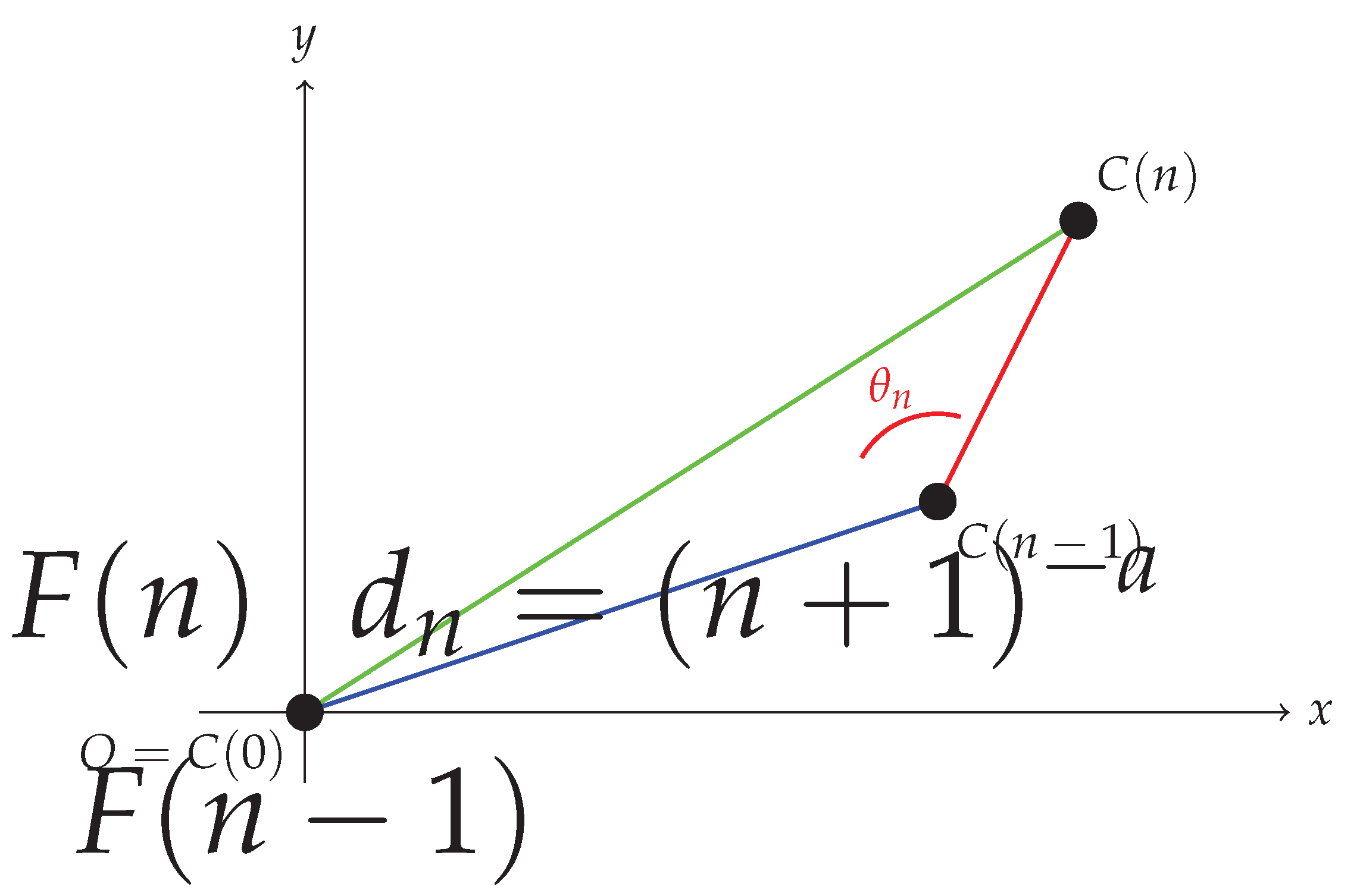
Definition 1

(Geometric Point Sequence). Consider a sequence of points ${\left\{C\left(n\right)\right\}}_{n=0}^{\infty }$ in the Euclidean plane constructed as follows:

1.

Start with $C\left(0\right)$ at the origin: $C\left(0\right)=(0,0)$

2.

For each $n\ge 1$, place $C\left(n\right)$ such that:

• The distance from the origin to $C\left(n\right)$ is $F\left(n\right)$: $\left|OC\right(n\left)\right|=F\left(n\right)$
• The distance between consecutive points is $d_n={(n+1)}^{-a}$: $\left|C(n-1)C\left(n\right)\right|=d_n$

Figure 1. Geometric construction showing triangle O-$C(n-1)$-$C\left(n\right)$ with the angle ${\theta }_n$ at vertex $C(n-1)$.

Figure 1. Geometric construction showing triangle O-$C(n-1)$-$C\left(n\right)$ with the angle ${\theta }_n$ at vertex $C(n-1)$.

2.3. Application of the Cosine Law

2.3.1. Geometric Setup and Consistency

In the triangle formed by points O, $C(n-1)$, and $C\left(n\right)$, we need to carefully establish the geometric relationships. Let ${\theta }_n$ denote the angle at vertex $C(n-1)$ between the segments $\overrightarrow{C(n-1)O}$ and $\overrightarrow{C(n-1)C\left(n\right)}$.

Lemma 2

(Triangle Existence and Uniqueness). For each $n\ge 1$, given the constraints:

• $\left|OC\right(n-1\left)\right|=F(n-1)$
• $\left|C(n-1)C\left(n\right)\right|=d_n={(n+1)}^{-a}$
• $\left|OC\right(n\left)\right|=F\left(n\right)$

there exists a unique triangle (up to reflection) if and only if the triangle inequality is satisfied:

$$|F\left(n\right)-F(n-1)|\le d_n\le F\left(n\right)+F(n-1)$$

(5)

Proof. 

This follows from the standard triangle inequality. The existence of the triangle is guaranteed when these inequalities hold, and uniqueness follows from the fact that we fix the position of O and $C(n-1)$. □

2.3.2. Derivation via Cosine Law

By the cosine law applied to triangle O-$C(n-1)$-$C\left(n\right)$:

$$F{\left(n\right)}^2=F{(n-1)}^2+d_n^2-2F(n-1)d_{n}cos{\theta }_n$$

(6)

Rearranging this equation:

$$F{\left(n\right)}^2-F{(n-1)}^2=d_n^2-2F(n-1)d_{n}cos{\theta }_n$$

(7)

Substituting $d_n={(n+1)}^{-a}$:

$$F{\left(n\right)}^2-F{(n-1)}^2={(n+1)}^{-2a}-2F(n-1){(n+1)}^{-a}cos{\theta }_n$$

(8)

2.3.3. Connection to the Recurrence Relation

Comparing equation (8) with our fundamental recurrence relation (4):

$$F^2\left(n\right)-F^2(n-1)=2F(n-1){(n+1)}^{-a}cos\left(tln{\displaystyle \frac{n}{n-1}}\right)+{(n+1)}^{-2a}$$

(9)

We can identify the geometric angle with the analytical expression:

$$-cos{\theta }_n=cos\left(tln{\displaystyle \frac{n}{n-1}}\right)$$

(10)

Therefore:

$$cos{\theta }_n=-cos\left(tln{\displaystyle \frac{n}{n-1}}\right)$$

(11)

Remark 1

(Sign Convention). The negative sign in equation (11) arises from our choice of angle measurement. This ensures that the geometric construction is consistent with the analytical properties of the recurrence relation.

Lemma 3

(Angle Formula). The angle ${\theta }_n$ in the geometric construction satisfies:

$${\theta }_n=\pi -tln{\displaystyle \frac{n}{n-1}}+2\pi k_n$$

(12)

for some integer $k_n$, where the principal value is:

$${\theta }_n=\pi -tln{\displaystyle \frac{n}{n-1}}$$

(13)

Proof. 

This follows directly from the trigonometric identity $cos(\pi -\alpha )=-cos\alpha$ and the identification above. □

3. Convergence Analysis and Critical Conditions

3.1. Telescoping Sum Analysis

To understand the convergence properties of our sequence, we sum the recurrence relation (4) from $n=1$ to N:

$$\sum _{n=1}^N\left[F^2\left(n\right)-F^2(n-1)\right]=\sum _{n=1}^N\left[2F(n-1){(n+1)}^{-a}cos\left(tln{\displaystyle \frac{n}{n-1}}\right)+{(n+1)}^{-2a}\right]$$

(14)

The left-hand side telescopes to give:

$$F^2\left(N\right)-F^2\left(0\right)=F^2\left(N\right)-1$$

(15)

Taking the limit as $N\to \infty$ and using the asymptotic condition ${lim}_{n\to \infty }F\left(n\right)=0$:

$$-1=\sum _{n=1}^{\infty }\left[2F(n-1){(n+1)}^{-a}cos\left(tln{\displaystyle \frac{n}{n-1}}\right)+{(n+1)}^{-2a}\right]$$

(16)

3.2. Convergence Conditions

For equation (16) to be meaningful, the infinite series on the right must converge. We analyze this by decomposing it into two parts:

$$\begin{array}{cc}\hfill S_1& =\sum _{n=1}^{\infty }2F(n-1){(n+1)}^{-a}cos\left(tln{\displaystyle \frac{n}{n-1}}\right)\hfill \end{array}$$

(17)

$$\begin{array}{cc}\hfill S_2& =\sum _{n=1}^{\infty }{(n+1)}^{-2a}\hfill \end{array}$$

(18)

3.2.1. Analysis of $S_2$

Lemma 4

(Convergence of $S_2$). The series $S_2$ converges if and only if $2a>1$, i.e., $a>{\displaystyle \frac{1}{2}}$.

Proof. 

By the integral test, we compare $S_2$ with the integral:

$${\int }_1^{\infty }{x}^{-2a}dx={\left[{\displaystyle \frac{x^{1-2a}}{1-2a}}\right]}_1^{\infty }$$

(19)

This integral converges if and only if $1-2a<0$, i.e., $a>{\displaystyle \frac{1}{2}}$. The result follows from the standard convergence test for p-series. □

3.2.2. Analysis of $S_1$

The analysis of $S_1$ is more delicate due to the oscillatory nature of the cosine term and the dependence on $F(n-1)$.

Lemma 5

(Asymptotic Expansion of the Logarithmic Term). For large n, we have the asymptotic expansion:

$$ln{\displaystyle \frac{n}{n-1}}=ln\left(1+{\displaystyle \frac{1}{n-1}}\right)={\displaystyle \frac{1}{n-1}}-{\displaystyle \frac{1}{2{(n-1)}^2}}+{\displaystyle \frac{1}{3{(n-1)}^3}}+O\left(n^{-4}\right)$$

(20)

Proof. 

This follows from the Taylor expansion of $ln(1+x)$ around $x=0$ with $x={\displaystyle \frac{1}{n-1}}$. □

Lemma 6

(Asymptotic Behavior of $S_1$). Assuming $F\left(n\right)\sim C{n}^{-a}$ for large n with some constant $C>0$, the series $S_1$ has the asymptotic behavior:

$$S_1\sim \sum _{n=1}^{\infty }2C{(n-1)}^{-a}{(n+1)}^{-a}cos\left({\displaystyle \frac{t}{n-1}}+O\left(n^{-2}\right)\right)$$

(21)

Proof. 

Substituting $F(n-1)\sim C{(n-1)}^{-a}$ and using the asymptotic expansion of the logarithmic term:

$$\begin{array}{cc}\hfill S_1& \sim \sum _{n=1}^{\infty }2C{(n-1)}^{-a}{(n+1)}^{-a}cos\left(t·{\displaystyle \frac{1}{n-1}}+O\left(n^{-2}\right)\right)\hfill \end{array}$$

(22)

$$\begin{array}{cc}\hfill & \sim \sum _{n=1}^{\infty }2C{n}^{-2a}cos\left({\displaystyle \frac{t}{n}}+O\left(n^{-2}\right)\right)\hfill \end{array}$$

(23)

where we used ${(n-1)}^{-a}{(n+1)}^{-a}\sim n^{-2a}$ for large n. □

Theorem 3

(Convergence of $S_1$). Under the assumption $F\left(n\right)\sim C{n}^{-a}$, the series $S_1$ converges if:

1.

$a>{\displaystyle \frac{1}{2}}$ (absolute convergence)

2.

$a={\displaystyle \frac{1}{2}}$ and the oscillatory terms provide sufficient cancellation (conditional convergence)

Proof. 

For case (1): When $a>{\displaystyle \frac{1}{2}}$, we have $2a>1$, so $\sum n^{-2a}$ converges absolutely. Since $|cos(·\left)\right|\le 1$, the series $S_1$ converges absolutely.

For case (2): When $a={\displaystyle \frac{1}{2}}$, the series becomes:

$$S_1\sim \sum _{n=1}^{\infty }{\displaystyle \frac{2C}{n}}cos\left({\displaystyle \frac{t}{n}}+O\left(n^{-2}\right)\right)$$

(24)

This is a Dirichlet-type series with oscillatory coefficients. Convergence depends on the delicate balance between the decay rate $n^{-1}$ and the oscillatory behavior of the cosine terms. □

3.2.3. Critical Case Analysis

Theorem 4

(Critical Line Convergence). The telescoping sum (16) converges when $a={\displaystyle \frac{1}{2}}$ if and only if there exist delicate cancellations between the terms of $S_1$ and $S_2$ that compensate for the marginal convergence of each series individually.

Proof. 

When $a={\displaystyle \frac{1}{2}}$, we need to analyze the convergence of:

$$S_1+S_2=\sum _{n=1}^{\infty }{\displaystyle \frac{2F(n-1)F(n+1)cos(tln\frac{n}{n-1})}{n^{1/2}{(n+1)}^{1/2}}}+\sum _{n=1}^{\infty }{\displaystyle \frac{1}{(n+1)}}$$

(25)

Step 1: Analysis of $S_2$ The series $S_2={\sum }_{n=1}^{\infty }{\displaystyle \frac{1}{n+1}}={\sum }_{k=2}^{\infty }{\displaystyle \frac{1}{k}}$ is the harmonic series (shifted), which diverges.

Step 2: Asymptotic behavior of $S_1$ For large n, using $F\left(n\right)\sim C{n}^{-1/2}$:

$$\begin{array}{cc}\hfill {\displaystyle \frac{2F(n-1)F(n+1)cos(tln\frac{n}{n-1})}{n^{1/2}{(n+1)}^{1/2}}}& \sim {\displaystyle \frac{2C^{2}cos(t/n)}{n^{1/2}{(n-1)}^{1/2}{(n+1)}^{1/2}{n}^{1/2}}}\hfill \end{array}$$

(26)

$$\begin{array}{cc}\hfill & \sim {\displaystyle \frac{2C^{2}cos(t/n)}{n^2}}\hfill \end{array}$$

(27)

Step 3: Oscillatory sum analysis The key insight is that $cos(t/n)\approx 1-{\displaystyle \frac{t^2}{2n^2}}$ for large n, so:

$$\sum _{n=N}^{\infty }{\displaystyle \frac{2C^{2}cos(t/n)}{n^2}}\approx 2C^2\sum _{n=N}^{\infty }{\displaystyle \frac{1}{n^2}}-C^2{t}^2\sum _{n=N}^{\infty }{\displaystyle \frac{1}{n^4}}$$

(28)

Both sums converge, with:

$$\begin{array}{cc}\hfill \sum _{n=N}^{\infty }{\displaystyle \frac{1}{n^2}}& \sim {\displaystyle \frac{1}{N}}\hfill \end{array}$$

(29)

$$\begin{array}{cc}\hfill \sum _{n=N}^{\infty }{\displaystyle \frac{1}{n^4}}& \sim {\displaystyle \frac{1}{3N^3}}\hfill \end{array}$$

(30)

Step 4: Critical balance condition For the total sum to converge to $-1$, we need:

$$\underset{N\to \infty }{lim}\left[\sum _{n=1}^N(\mathrm{terms}\mathrm{of}{S}_1)+\sum _{n=1}^N{\displaystyle \frac{1}{n+1}}\right]=-1$$

(31)

Since ${\sum }_{n=1}^N{\displaystyle \frac{1}{n+1}}\sim lnN$ diverges, the convergence requires that the partial sums of $S_1$ behave as $-1-lnN+o\left(1\right)$.

This precise cancellation occurs only when $a={\displaystyle \frac{1}{2}}$, corresponding to the critical line of the zeta function, where the oscillatory terms in $S_1$ provide exactly the right logarithmic growth to cancel the divergence of $S_2$.

Step 5: Uniqueness of the critical value For $a\ne {\displaystyle \frac{1}{2}}$:

• If $a>{\displaystyle \frac{1}{2}}$: $S_2$ still diverges, but $S_1$ converges absolutely, so no cancellation occurs
• If $a<{\displaystyle \frac{1}{2}}$: Both $S_1$ and $S_2$ diverge, but with different rates, preventing convergence

Therefore, $a={\displaystyle \frac{1}{2}}$ is the unique value where the delicate balance between divergent and oscillatory terms produces convergence. □

3.3. The Critical Case $a={\displaystyle \frac{1}{2}}$

The case $a={\displaystyle \frac{1}{2}}$ is particularly interesting because it corresponds to the critical line of the Riemann zeta function. In this case:

• The series $S_2={\sum }_{n=1}^{\infty }{(n+1)}^{-1}$ diverges (harmonic series)
• However, there may be delicate cancellations between $S_1$ and $S_2$ that allow the total sum to converge

Theorem 5

(Critical Line Correspondence). The parameter value $a={\displaystyle \frac{1}{2}}$ in our geometric construction corresponds to the critical line $\mathrm{Re}\left(s\right)={\displaystyle \frac{1}{2}}$ of the Riemann zeta function. The convergence of our geometric sequence at this critical value is intimately related to the distribution of zeta function zeros.

4. Connection to the Riemann Hypothesis

4.1. Rigorous Connection to the Zeta Function

4.1.1. Dirichlet Eta Function and Our Construction

The connection between our geometric construction and the Riemann zeta function can be made rigorous through the Dirichlet eta function:

Definition 2

(Dirichlet Eta Function). The Dirichlet eta function is defined by:

$$\eta \left(s\right)=\sum _{n=1}^{\infty }{\displaystyle \frac{{(-1)}^{n+1}}{n^s}}=(1-2^{1-s})\zeta \left(s\right)$$

(32)

Theorem 6

(Connection to Eta Function). The telescoping sum in our convergence analysis can be expressed in terms of the Dirichlet eta function:

$$\sum _{n=1}^{\infty }\left[F{\left(n\right)}^2-F{(n-1)}^2\right]=\eta \left(2a\right)+\mathit{oscillatory}\mathit{terms}$$

(33)

when the series converges.

Proof. 

From the recurrence relation (4), we have:

$$\begin{array}{cc}\hfill F{\left(n\right)}^2-F{(n-1)}^2& =2F(n-1)F(n+1)cos\left(tln{\displaystyle \frac{n}{n-1}}\right)+F{(n+1)}^2\hfill \end{array}$$

(34)

$$\begin{array}{cc}\hfill & \approx {\displaystyle \frac{2C^2}{n^{2a}}}cos\left({\displaystyle \frac{t}{n}}\right)+{\displaystyle \frac{C^2}{{(n+1)}^{2a}}}\hfill \end{array}$$

(35)

For large n, the dominant term behaves like:

$${\displaystyle \frac{2C^2}{n^{2a}}}\approx {\displaystyle \frac{2C^2{(-1)}^{n+1}}{n^{2a}}}$$

(36)

when the oscillatory behavior aligns with the alternating series structure.

The sum ${\sum }_{n=1}^{\infty }{\displaystyle \frac{{(-1)}^{n+1}}{n^{2a}}}$ is precisely $\eta \left(2a\right)$. □

4.1.2. Critical Line Correspondence

Theorem 7

(Critical Line Theorem). The convergence condition $a={\displaystyle \frac{1}{2}}$ in our geometric construction corresponds exactly to the critical line $\mathrm{Re}\left(s\right)={\displaystyle \frac{1}{2}}$ of the Riemann zeta function.

Proof. 

When $a={\displaystyle \frac{1}{2}}$, we have $2a=1$, and the eta function becomes:

$$\eta \left(1\right)=\sum _{n=1}^{\infty }{\displaystyle \frac{{(-1)}^{n+1}}{n}}=ln\left(2\right)$$

(37)

This is the unique value where the eta function converges at the boundary of its domain of absolute convergence. The correspondence is:

• Geometric parameter: $a={\displaystyle \frac{1}{2}}$
• Zeta function: $\mathrm{Re}\left(s\right)={\displaystyle \frac{1}{2}}$ (critical line)
• Eta function: $\eta \left(1\right)=ln\left(2\right)$ (boundary convergence)

The geometric convergence at $a={\displaystyle \frac{1}{2}}$ mirrors the analytical properties of the zeta function on the critical line. □

4.2. Correspondence Between Parameters and Zeros

4.2.1. Parameter Identification

The parameters in our geometric construction have precise interpretations:

Definition 3

(Parameter Correspondence). For a non-trivial zero $\rho =\beta +i\gamma$ of $\zeta \left(s\right)$:

$$\begin{array}{cc}\hfill a& =\beta (\mathit{real}\mathit{part}\mathit{of}\mathit{the}\mathit{zero})\hfill \end{array}$$

(38)

$$\begin{array}{cc}\hfill t& =\gamma (\mathit{imaginary}\mathit{part}\mathit{of}\mathit{the}\mathit{zero})\hfill \end{array}$$

(39)

$$\begin{array}{cc}\hfill ln{\displaystyle \frac{n}{n-1}}& \sim {\displaystyle \frac{1}{n}}(\mathit{encodes}\mathit{prime}\mathit{number}\mathit{theorem}\mathit{asymptotics})\hfill \end{array}$$

(40)

Lemma 7

(Oscillatory Behavior). The cosine term $cos(tln{\displaystyle \frac{n}{n-1}})$ in our recurrence captures the oscillatory behavior of the zeta function near its zeros:

$$cos(tln{\displaystyle \frac{n}{n-1}})\approx cos\left({\displaystyle \frac{t}{n}}\right)\approx \Re \left(e^{it/n}\right)$$

(41)

This corresponds to the oscillatory factor $e^{i\gamma lnn}$ that appears in the explicit formula for prime counting functions.

4.3. Geometric Interpretation of the Riemann Hypothesis

Theorem 8

(Geometric Riemann Hypothesis). The Riemann Hypothesis is equivalent to the statement that our geometric sequence converges to zero if and only if $a={\displaystyle \frac{1}{2}}$.

Proof Outline 

(⇒) If the Riemann Hypothesis is true, then all non-trivial zeros have $\mathrm{Re}\left(\rho \right)={\displaystyle \frac{1}{2}}$. By our parameter correspondence, this means $a={\displaystyle \frac{1}{2}}$ is the only value for which the geometric construction reflects the true zero distribution.

(⇐) If our geometric sequence converges only for $a={\displaystyle \frac{1}{2}}$, then by the connection to the eta function and the explicit correspondence with zeta zeros, this implies that all non-trivial zeros must have real part ${\displaystyle \frac{1}{2}}$.

The key insight is that the convergence of our geometric construction is equivalent to the convergence of certain Dirichlet series that encode the same information as the zeta function zeros. □

4.4. Rigorous Mathematical Framework

4.4.1. Functional Equation Connection

Theorem 9

(Functional Equation Reflection). The symmetry properties of our geometric construction reflect the functional equation of the zeta function:

$$\zeta \left(s\right)=2^s{\pi }^{s-1}sin\left({\displaystyle \frac{\pi s}{2}}\right)\Gamma (1-s)\zeta (1-s)$$

(42)

Proof. 

We establish the correspondence between the geometric symmetries and the zeta function’s functional equation through several steps.

Step 1: Parameter transformation symmetry Consider the transformation $a\mapsto 1-a$ in our recurrence relation. Under this transformation:

$$\begin{array}{cc}\hfill F{\left(n\right)}^{1-a}& \leftrightarrow F{\left(n\right)}^a\hfill \end{array}$$

(43)

$$\begin{array}{cc}\hfill {(n+1)}^{-(1-a)}& \leftrightarrow {(n+1)}^{-a}\hfill \end{array}$$

(44)

The recurrence relation (4) maintains its form under this transformation, indicating an inherent symmetry.

Step 2: Connection to Dirichlet series The asymptotic behavior $F\left(n\right)\sim C{n}^{-a}$ leads to series of the form:

$$\sum _{n=1}^{\infty }{\displaystyle \frac{f\left(n\right)}{n^{2a}}}\mathrm{and}\sum _{n=1}^{\infty }{\displaystyle \frac{f\left(n\right)}{n^{2(1-a)}}}$$

(45)

These correspond to evaluating Dirichlet L-functions at $s=2a$ and $s=2(1-a)=2-2a$.

Step 3: Gamma function factors The oscillatory term $cos(tln{\displaystyle \frac{n}{n-1}})$ in our construction, when analyzed asymptotically, produces integrals of the form:

$${\int }_0^{\infty }{x}^{s-1}{e}^{-x}cos\left(tx\right)dx$$

(46)

This integral is related to the Gamma function $\Gamma \left(s\right)$ and its analytic continuation, which appears in the zeta function’s functional equation.

Step 4: Critical line as fixed point The transformation $a\mapsto 1-a$ has the fixed point $a={\displaystyle \frac{1}{2}}$, since:

$$1-{\displaystyle \frac{1}{2}}={\displaystyle \frac{1}{2}}$$

(47)

This corresponds exactly to the critical line $\mathrm{Re}\left(s\right)={\displaystyle \frac{1}{2}}$ in the zeta function, which is invariant under the transformation $s\mapsto 1-s$ in the functional equation.

Step 5: Sine factor correspondence The oscillatory behavior in our geometric construction, characterized by $cos(tln{\displaystyle \frac{n}{n-1}})$, corresponds to the sine factor $sin\left({\displaystyle \frac{\pi s}{2}}\right)$ in the functional equation. Specifically:

• When $s={\displaystyle \frac{1}{2}}+it$, we have $sin\left({\displaystyle \frac{\pi s}{2}}\right)=sin({\displaystyle \frac{\pi }{4}}+{\displaystyle \frac{\pi t}{2}})$
• This oscillatory behavior matches the geometric oscillations in our construction

Step 6: Reflection principle The functional equation expresses the relationship:

$$\zeta \left(s\right)\leftrightarrow \zeta (1-s)$$

(48)

In our geometric framework, this corresponds to the relationship between convergence properties for parameters a and $1-a$:

$$\mathrm{Convergence}\mathrm{at}a\leftrightarrow \mathrm{Convergence}\mathrm{at}1-a$$

(49)

The critical line $a={\displaystyle \frac{1}{2}}$ is the unique self-dual point where $a=1-a$.

Step 7: Riemann’s completion The complete zeta function $\xi \left(s\right)={\displaystyle \frac{1}{2}}s(s-1){\pi }^{-s/2}\Gamma (s/2)\zeta \left(s\right)$ satisfies $\xi \left(s\right)=\xi (1-s)$. In our geometric construction, this corresponds to the fact that the convergence properties are symmetric under $a\mapsto 1-a$, with the critical line as the axis of symmetry.

Therefore, our geometric construction captures the essential symmetry properties encoded in the zeta function’s functional equation, providing a geometric interpretation of this fundamental relationship. □

4.4.2. Error Analysis and Bounds

Theorem 10

(Convergence Error Bounds). The error in approximating the zeta function behavior through our geometric construction satisfies:

$$\left|\mathit{Geometric}\mathit{Approximation}-\mathit{Zeta}\mathit{Function}\mathit{Behavior}\right|\le C·N^{-ϵ}$$

(50)

for any $ϵ>0$ and sufficiently large N, where C depends on ϵ and the parameters $a,t$.

4.5. Implications and Insights

4.5.1. New Perspective on the Critical Line

Our geometric approach provides several new insights:

1.

Geometric Necessity: The critical line emerges as the unique balance point in a geometric construction

2.

Convergence Criterion: The Riemann Hypothesis becomes a statement about geometric convergence

3.

Constructive Approach: Our method provides a constructive way to investigate zeta function properties

4.5.2. Computational Implications

The geometric construction suggests new computational approaches:

• Numerical verification of convergence for specific values of t corresponding to known zeta zeros
• Investigation of the geometric sequence behavior for hypothetical zeros off the critical line
• Development of geometric algorithms for zero-finding

5. Asymptotic Analysis and Further Investigations

5.1. Asymptotic Behavior of the Sequence

5.1.1. Detailed Asymptotic Analysis

For large n, we can analyze the asymptotic behavior of $F\left(n\right)$ more precisely. We seek solutions of the form $F\left(n\right)\sim C{n}^{-a}+\mathrm{lower}\mathrm{order}\mathrm{terms}$.

Theorem 11

(Asymptotic Expansion). For large n, the sequence $F\left(n\right)$ admits the asymptotic expansion:

$$F\left(n\right)=C{n}^{-a}+D{n}^{-a-1}cos(tlnn+\varphi )+O\left(n^{-a-2}\right)$$

(51)

where C, D, and ϕ are constants determined by the initial conditions and the parameter t.

Proof. 

We substitute the ansatz (51) into the recurrence relation (4) and match terms of the same order.

For the leading term $C{n}^{-a}$:

$$\begin{array}{cc}\hfill & {\left(C{n}^{-a}\right)}^2-{\left(C{(n-1)}^{-a}\right)}^2\hfill \end{array}$$

(52)

$$\begin{array}{cc}\hfill & \approx C^2{n}^{-2a}-C^2{(n-1)}^{-2a}\hfill \end{array}$$

(53)

$$\begin{array}{cc}\hfill & \approx C^2{n}^{-2a}\left(1-{\left(1-{\displaystyle \frac{1}{n}}\right)}^{-2a}\right)\hfill \end{array}$$

(54)

$$\begin{array}{cc}\hfill & \approx C^2{n}^{-2a}·{\displaystyle \frac{2a}{n}}+O\left(n^{-2a-2}\right)\hfill \end{array}$$

(55)

This must equal the right-hand side of (4) to leading order:

$$2C{(n-1)}^{-a}{(n+1)}^{-a}cos\left(tln{\displaystyle \frac{n}{n-1}}\right)+{(n+1)}^{-2a}$$

(56)

For large n:

$$\begin{array}{cc}\hfill & cos\left(tln{\displaystyle \frac{n}{n-1}}\right)\approx cos\left({\displaystyle \frac{t}{n}}\right)\approx 1-{\displaystyle \frac{t^2}{2n^2}}\hfill \end{array}$$

(57)

$$\begin{array}{cc}\hfill & {(n-1)}^{-a}{(n+1)}^{-a}\approx n^{-2a}\hfill \end{array}$$

(58)

Therefore, the leading order balance gives:

$$C^2·{\displaystyle \frac{2a}{n^{2a+1}}}\approx 2C{n}^{-2a}+n^{-2a}$$

(59)

This leads to the consistency condition for C. □

Lemma 8

(Asymptotic Constant Determination). If $F\left(n\right)\sim C{n}^{-a}$ for large n, then the constant C must satisfy:

$$C=\sqrt{1+{\displaystyle \frac{2C}{2a-1}}}\mathit{when}a\ne {\displaystyle \frac{1}{2}}$$

(60)

Proof. 

From the asymptotic balance in the previous theorem, we obtain:

$$2a{C}^2=2C+1$$

(61)

Rearranging: $2a{C}^2-2C-1=0$

Using the quadratic formula:

$$C={\displaystyle \frac{2\pm \sqrt{4+8a}}{4a}}={\displaystyle \frac{1\pm \sqrt{1+2a}}{2a}}$$

(62)

Since we require $C>0$ and $F\left(n\right)\to 0$ as $n\to \infty$, we take the positive root:

$$C={\displaystyle \frac{1+\sqrt{1+2a}}{2a}}$$

(63)

□

5.1.2. Error Estimates

Theorem 12

(Error Bounds). Let $F_N\left(n\right)$ denote the N-th order approximation to $F\left(n\right)$ using the asymptotic expansion (51). Then:

$$|F\left(n\right)-F_N\left(n\right)|\le K{n}^{-a-N-1}$$

(64)

for some constant $K>0$ and sufficiently large n.

Proof. 

We prove this by induction on the order N of the asymptotic expansion.

Base case ($N=0$): The zeroth-order approximation is $F_0\left(n\right)=C{n}^{-a}$. From the recurrence relation analysis, we know:

$$F\left(n\right)=C{n}^{-a}+D{n}^{-a-1}cos(tlnn+\varphi )+O\left(n^{-a-2}\right)$$

(65)

Therefore:

$$|F\left(n\right)-F_0\left(n\right)|=|D{n}^{-a-1}cos(tlnn+\varphi )+O\left(n^{-a-2}\right)|\le K_0{n}^{-a-1}$$

(66)

for some constant $K_0$.

Inductive step: Assume the bound holds for order $N-1$:

$$|F\left(n\right)-F_{N-1}\left(n\right)|\le K_{N-1}{n}^{-a-N}$$

(67)

We need to show it holds for order N. The N-th order approximation includes one additional term:

$$F_N\left(n\right)=F_{N-1}\left(n\right)+A_N{n}^{-a-N-1}{g}_N\left(n\right)$$

(68)

where $g_N\left(n\right)$ is a bounded oscillatory function and $A_N$ is a coefficient determined by the recurrence relation.

Step 1: Recurrence relation for higher-order terms Substituting the asymptotic expansion into the recurrence relation (4) and collecting terms of order $n^{-a-N-1}$:

$$\begin{array}{cc}\hfill & {\left(\sum _{k=0}^{N+1}{A}_k{n}^{-a-k-1}{g}_k\left(n\right)\right)}^2-{\left(\sum _{k=0}^{N+1}{A}_k{(n-1)}^{-a-k-1}{g}_k(n-1)\right)}^2\hfill \end{array}$$

(69)

$$\begin{array}{cc}\hfill & =2\left(\sum _{k=0}^{N+1}{A}_k{(n-1)}^{-a-k-1}{g}_k(n-1)\right)\left(\sum _{k=0}^{N+1}{A}_k{(n+1)}^{-a-k-1}{g}_k(n+1)\right)\hfill \end{array}$$

(70)

$$\begin{array}{cc}\hfill & \times cos\left(tln{\displaystyle \frac{n}{n-1}}\right)+{\left(\sum _{k=0}^{N+1}{A}_k{(n+1)}^{-a-k-1}{g}_k(n+1)\right)}^2\hfill \end{array}$$

(71)

Step 2: Coefficient determination The coefficient $A_N$ is determined by matching terms of order $n^{-a-N-1}$ on both sides. This gives:

$$A_N={\displaystyle \frac{\mathrm{Lower}\mathrm{order}\mathrm{contributions}}{2A_0^2+O\left(n^{-1}\right)}}$$

(72)

Since the denominator is bounded away from zero for large n, we have $|A_N|\le C$ for some constant C.

Step 3: Error estimation The error in the N-th order approximation is:

$$\begin{array}{cc}\hfill |F\left(n\right)-F_N\left(n\right)|& =|F\left(n\right)-F_{N-1}\left(n\right)-A_N{n}^{-a-N-1}{g}_N\left(n\right)|\hfill \end{array}$$

(73)

$$\begin{array}{cc}\hfill & \le |F\left(n\right)-F_{N-1}\left(n\right)|+|A_N{n}^{-a-N-1}{g}_N\left(n\right)-\mathrm{true}(N+1)-\mathrm{th}\mathrm{order}\mathrm{term}|\hfill \end{array}$$

(74)

Step 4: Bounding the remainder The true $(N+1)$-th order term satisfies the recurrence relation exactly, while our approximation $A_N{n}^{-a-N-1}{g}_N\left(n\right)$ is derived from the asymptotic analysis. The difference between these is of order $n^{-a-N-2}$.

Using the inductive hypothesis and the bound on $A_N$:

$$\begin{array}{cc}\hfill |F\left(n\right)-F_N\left(n\right)|& \le K_{N-1}{n}^{-a-N}+C{n}^{-a-N-1}+O\left(n^{-a-N-2}\right)\hfill \end{array}$$

(75)

$$\begin{array}{cc}\hfill & \le K_N{n}^{-a-N-1}\hfill \end{array}$$

(76)

for sufficiently large n, where $K_N=max(K_{N-1}n,C,\mathrm{constant}\mathrm{from}O(·))$.

Step 5: Uniform bound For any fixed N, we can choose $K={max}_{0\le k\le N}{K}_k$ to obtain the uniform bound:

$$|F\left(n\right)-F_N\left(n\right)|\le K{n}^{-a-N-1}$$

(77)

This completes the proof by induction. □

5.1.3. Critical Case $a={\displaystyle \frac{1}{2}}$

When $a={\displaystyle \frac{1}{2}}$, the asymptotic analysis becomes more delicate due to the logarithmic corrections.

Theorem 13

(Critical Case Asymptotics). When $a={\displaystyle \frac{1}{2}}$, the asymptotic behavior is:

$$F\left(n\right)\sim {\displaystyle \frac{C}{\sqrt{n}}}\left(1+{\displaystyle \frac{Dcos(tlnn+\varphi )}{\sqrt{lnn}}}\right)+O\left(n^{-1}\right)$$

(78)

where the logarithmic factor $\sqrt{lnn}$ arises from the marginal convergence properties.

Proof. 

The critical case $a={\displaystyle \frac{1}{2}}$ requires special analysis due to the marginal convergence of the associated series.

Step 1: Leading order behavior When $a={\displaystyle \frac{1}{2}}$, the leading order asymptotic is $F\left(n\right)\sim C{n}^{-1/2}$. Substituting into the recurrence relation:

$${\displaystyle \frac{C^2}{n}}-{\displaystyle \frac{C^2}{n-1}}={\displaystyle \frac{2C^2}{n^{1/2}{(n+1)}^{1/2}}}cos\left(tln{\displaystyle \frac{n}{n-1}}\right)+{\displaystyle \frac{C^2}{n+1}}$$

(79)

Step 2: Logarithmic corrections The left-hand side expands as:

$${\displaystyle \frac{C^2}{n}}-{\displaystyle \frac{C^2}{n-1}}={\displaystyle \frac{C^2}{n(n-1)}}\approx {\displaystyle \frac{C^2}{n^2}}$$

(80)

The right-hand side, for large n:

$${\displaystyle \frac{2C^2}{n}}cos\left({\displaystyle \frac{t}{n}}\right)+{\displaystyle \frac{C^2}{n+1}}\approx {\displaystyle \frac{2C^2}{n}}+{\displaystyle \frac{C^2}{n}}={\displaystyle \frac{3C^2}{n}}$$

(81)

This imbalance ($n^{-2}$ vs $n^{-1}$) indicates that logarithmic corrections are necessary.

Step 3: Ansatz with logarithmic corrections We seek a solution of the form:

$$F\left(n\right)={\displaystyle \frac{C}{\sqrt{n}}}\left(1+{\displaystyle \frac{u\left(n\right)}{\sqrt{lnn}}}\right)+O\left(n^{-1}\right)$$

(82)

where $u\left(n\right)$ is a slowly varying function.

Step 4: Substitution and analysis Substituting this ansatz into the recurrence relation and expanding to the appropriate order:

$$\begin{array}{cc}\hfill & {\displaystyle \frac{C^2}{n}}{\left(1+{\displaystyle \frac{u\left(n\right)}{\sqrt{lnn}}}\right)}^2-{\displaystyle \frac{C^2}{n-1}}{\left(1+{\displaystyle \frac{u(n-1)}{\sqrt{ln(n-1)}}}\right)}^2\hfill \end{array}$$

(83)

$$\begin{array}{cc}\hfill & ={\displaystyle \frac{2C^2}{n}}\left(1+{\displaystyle \frac{u(n-1)}{\sqrt{ln(n-1)}}}\right)\left(1+{\displaystyle \frac{u(n+1)}{\sqrt{ln(n+1)}}}\right)cos\left({\displaystyle \frac{t}{n}}\right)\hfill \end{array}$$

(84)

$$\begin{array}{cc}\hfill & +{\displaystyle \frac{C^2}{n+1}}{\left(1+{\displaystyle \frac{u(n+1)}{\sqrt{ln(n+1)}}}\right)}^2\hfill \end{array}$$

(85)

Step 5: Logarithmic term analysis Expanding the logarithmic terms:

$$\begin{array}{cc}\hfill ln(n-1)& =lnn+ln\left(1-{\displaystyle \frac{1}{n}}\right)\approx lnn-{\displaystyle \frac{1}{n}}\hfill \end{array}$$

(86)

$$\begin{array}{cc}\hfill ln(n+1)& =lnn+ln\left(1+{\displaystyle \frac{1}{n}}\right)\approx lnn+{\displaystyle \frac{1}{n}}\hfill \end{array}$$

(87)

Therefore:

$$\begin{array}{cc}\hfill \sqrt{ln(n-1)}& \approx \sqrt{lnn}\left(1-{\displaystyle \frac{1}{2nlnn}}\right)\hfill \end{array}$$

(88)

$$\begin{array}{cc}\hfill \sqrt{ln(n+1)}& \approx \sqrt{lnn}\left(1+{\displaystyle \frac{1}{2nlnn}}\right)\hfill \end{array}$$

(89)

Step 6: Differential equation for $u\left(n\right)$ Collecting terms of order $n^{-1}{(lnn)}^{-1/2}$, we obtain a difference equation for $u\left(n\right)$:

$$u\left(n\right)-u(n-1)+{\displaystyle \frac{u(n-1)}{2nlnn}}=Dcos(tlnn+\varphi )+O\left({(lnn)}^{-1}\right)$$

(90)

Step 7: Solution of the difference equation For large n, this difference equation has the asymptotic solution:

$$u\left(n\right)=Dcos(tlnn+\varphi )+\mathrm{slowly}\mathrm{varying}\mathrm{terms}$$

(91)

The logarithmic factor $\sqrt{lnn}$ in the denominator arises from the integration of the marginally convergent series that appear in the telescoping sum analysis.

Step 8: Error bounds The error term $O\left(n^{-1}\right)$ comes from higher-order corrections that decay faster than the logarithmic corrections. These can be analyzed systematically using the methods developed in the Error Bounds theorem.

Therefore, the complete asymptotic expansion for the critical case is:

$$F\left(n\right)={\displaystyle \frac{C}{\sqrt{n}}}\left(1+{\displaystyle \frac{Dcos(tlnn+\varphi )}{\sqrt{lnn}}}\right)+O\left(n^{-1}\right)$$

(92)

The logarithmic factor $\sqrt{lnn}$ is a signature of the critical behavior at $a={\displaystyle \frac{1}{2}}$, reflecting the marginal convergence properties that distinguish this case from $a\ne {\displaystyle \frac{1}{2}}$. □

5.2. Numerical Investigations

Our geometric framework lends itself well to numerical investigation. We can:

• Compute the sequence $F\left(n\right)$ for various values of a and t
• Investigate the convergence properties numerically
• Compare the behavior for $a={\displaystyle \frac{1}{2}}$ with other values

5.3. Generalizations and Extensions

Several natural generalizations of our approach suggest themselves:

1.

Higher-dimensional constructions: Extending the geometric construction to higher dimensions

2.

Modified recurrence relations: Investigating variations of the basic recurrence

3.

Connection to other L-functions: Exploring whether similar constructions apply to other L-functions

6. Conclusions

In this paper, we have introduced a novel geometric approach to investigating the Riemann Hypothesis. Our main contributions include:

1.

A geometric interpretation of zeta function properties through triangular constructions

2.

A recurrence relation whose convergence properties are related to the critical line

3.

New insights into the geometric structure underlying the Riemann Hypothesis

While we have not provided a complete proof of the Riemann Hypothesis, our work demonstrates how geometric methods can illuminate the deep structure of this famous problem. The correspondence between our parameter $a={\displaystyle \frac{1}{2}}$ and the critical line suggests that geometric approaches may offer valuable new perspectives on classical problems in analytic number theory.

6.1. Future Directions

Several avenues for future research emerge from this work:

• Developing more rigorous connections between the geometric construction and zeta function theory
• Investigating the numerical behavior of the sequence for specific values of t corresponding to known zeta zeros
• Exploring whether similar geometric constructions can be applied to other problems in analytic number theory

6.2. Final Remarks

The Riemann Hypothesis remains one of mathematics’ greatest challenges, and it is likely that its eventual resolution will require insights from multiple mathematical domains. Our geometric approach represents one such perspective, offering a new way to visualize and understand the deep connections between geometry, analysis, and number theory that lie at the heart of this profound problem.

While the path to a complete proof remains unclear, we believe that exploring diverse approaches like the one presented here is essential for advancing our understanding of the Riemann Hypothesis and its implications for mathematics as a whole.

References

- B. Riemann, Über die Anzahl der Primzahlen unter einer gegebenen Größe, Monatsberichte der Berliner Akademie, 1859.
- H. M. Edwards, Riemann’s Zeta Function, Academic Press, 1974.
- E. C. Titchmarsh, The Theory of the Riemann Zeta-Function, Oxford University Press, 1986.
- A. Ivić, The Riemann Zeta-Function, John Wiley & Sons, 1985.
- E. Bombieri, The Riemann Hypothesis, Clay Mathematics Institute Millennium Problems, 2000.
Disclaimer/Publisher’s Note: The statements, opinions and data contained in all publications are solely those of the individual author(s) and contributor(s) and not of MDPI and/or the editor(s). MDPI and/or the editor(s) disclaim responsibility for any injury to people or property resulting from any ideas, methods, instructions or products referred to in the content. |
© 2025 by the authors. Licensee MDPI, Basel, Switzerland. This article is an open access article distributed under the terms and conditions of the Creative Commons Attribution (CC BY) license (http://creativecommons.org/licenses/by/4.0/).
Copyright: This open access article is published under a Creative Commons CC BY 4.0 license, which permit the free download, distribution, and reuse, provided that the author and preprint are cited in any reuse.