Submitted:
10 October 2025
Posted:
11 October 2025
You are already at the latest version
Abstract
Although access to quality public spaces encourages physical activity (PA), their unequal distribution can exacerbate social inequalities. This study examined the relationship between the availability of spaces for PA and social marginalization in urban Basic Geostatistical Areas (Spanish acronym AGEB) in Mexico, using national databases on urban facilities and demographics. Space densities for PA were calculated by AGEB, and the bivariate Moran’s I and LISA methodology were followed to identify global and local patterns. A weak negative spatial correlation was detected (I = −0.006) at the national level, with clusters of AGEBs with low marginalization and low density of spaces for PA. Contrasts were observed between the three most populated metropolitan areas, with Mexico City and Guadalajara showing significant positive correlations, while Monterrey exhibited a different pattern. The urban furniture earmarked for PA is insufficient and its distribution reproduces socio-spatial inequalities. The dynamics differ across metropolises, underscoring the need for localized policies that will prioritize the provision of public spaces in marginalized communities.
Keywords:
public spaces
; physical activity
; social marginalization
; spatial analysis
; environmental justice
1. Introduction
Access to quality public spaces is an essential feature for encouraging physical activity and enhancing public well-being. Physical activity improves physical health as it is associated with a lower risk of developing obesity, cardiovascular disease and diabetes [1], and has positive effects on emotional well-being, since it reduces anxiety, depression, and stress, and encourages the development of intellectual and cognitive skills [2,3]. Access to parks or green areas has been linked to greater physical activity in children, adolescents [4,5] and adults [6], albeit not consistently. In children and adolescents, the availability of public spaces tends to be associated with more time for spontaneous or free outdoor play [5].
Urban planning guaranteeing equitable access to public spaces for physical activity could therefore contribute to the reduction of non-communicable diseases, mental health promotion and the strengthening of the social fabric while effectively managing the high degree of urbanization [7]. In Mexico, 82.1% of the population currently live in urban areas [8]. However, in many of its cities, distribution of these public spaces is not equitable, potentially creating barriers to physical activity in vulnerable populations [9,10]. Planning gaps fail to place people at the center of decision-making to improve their access to and exercise of their human rights, including the right to health.
Disparities in access to spaces for physical activity can contribute to social inequalities in health-related behaviors [11]. Although there are different forms of physical activity, in the urban context, recreational activity is the most important one, since people nowadays spend less time on occupations or forms of transportation requiring physical effort. Studies have consistently shown a correlation between higher socioeconomic status and greater engagement in recreational physical activity [12].
Socioeconomic disparities in the availability of green spaces in Mexico City have previously been analyzed [13,14,15]. These studies show that the availability of green spaces tends to be lower in the most marginalized basic geostatistical areas (AGEB). However, these studies have certain limitations, one of which is that they only considered the state of Mexico City, which is part of the Mexico City Metropolitan Area (MCMA). The MCMA includes municipalities from three states (Mexico City, Mexico State, and Hidalgo), which are socially and historically intertwined. Excluding municipalities in Mexico State and Hidalgo from the analysis means that large areas with the worst living conditions in the MCMA were overlooked. Another limitation of this research is that other cities or metropolitan areas were not included. Although Mexico City is one of the states with the largest population, there are other sizable metropolitan areas, including 14 with populations exceeding one million inhabitants [16]. Although green areas are not equivalent to public spaces for PA, many of them are suitable for this use.
Equitable access to spaces for physical activity must be addressed from a social and environmental justice perspective, since urban design can reinforce or mitigate structural inequalities in health and mobility [17]. Spatial analysis provides tools for examining the geographical distribution of public spaces and their relationship with health and other factors such as social marginalization. Geographic information systems (GIS) can identify patterns of inequality in urban infrastructure and their impact on health equity [11]. The objective of the study is to analyze the spatial distribution and availability of public spaces for PA in urban AGEBs in Mexico and their relationship with social marginalization at the AGEB level.
2. Materials and Methods
Public spaces for PA were identified through the INEGI National Geostatistical Framework [18] and OpenStreetMap (for 2024). The National Geostatistical Framework is designed to reference statistical information from INEGI censuses and surveys [19]. In keeping with the Framework, green areas and medians in urban areas with information updated to 2020 were classified as public spaces for PA. Places associated with public space such as courts, stadiums, gardens, parks, sports units, recreational areas, and green areas were also considered. This information was supplemented by information from the OSM, a publicly accessible tool that is continuously updated with contributions from users. We used information collected in April 2024. Due to the different classifications adopted by OSM, places it classified as parks, fields, and meadows, and points of interest designated as parks were considered public spaces for PA. To avoid duplication in the associated data from the National Geostatistical Framework and OSM, the database was filtered to ensure that only single values for physical activity spaces were included.
The study explores urban areas using the AGEB as the unit of analysis because it is the spatial scale that best describes the availability of public spaces for PA in the everyday dynamics of the population. At the same time, only urban AGEBs are studied, because the quality of the information from both the National Geostatistical Framework and the OSM is usually more reliable for these types of settlements than for rural AGEBs. A total of 66,422 urban AGEBs were identified.
To ensure that the analysis was based on AGEBs with a resident population and explored the surroundings in which this population lived, the AGEBs were divided into quintiles according to the number of inhabited dwellings registered in the 2020 INEGI Population and Housing Census [19]. AGEBs found in the first quintile, in other words, those that had between 0 and 22 inhabited dwellings, were excluded. The final number of urban AGEBs analyzed was 50,372.
Once the public spaces for PA and the main urban AGEBs inhabited by the population had been determined, the density of public spaces for PA in each AGEB was calculated as the quotient of the number of square meters of public spaces for PA divided by the total population residing in that AGEB, multiplied by 100.
The level of marginalization considered is the 2020 Urban Marginalization Index reported by the National Population Council at the AGEB level [20]. The index was developed from the socioeconomic indicators in the 2020 Population and Housing Census, such as the percentages of the population between the ages of six and 14 who do not attend school, the population aged 15 or older who do not have basic education, the population without state health insurance, and occupants of private homes lacking drainage, toilets, electricity, and piped water, with dirt floors, overcrowding, and no refrigerator, internet, or cell phone [20]. A higher level on the 2020 marginalization index indicates that the corresponding AGEB has less social marginalization.
Quartiles were created from the marginalization index for each metropolitan area. The means and medians of the density of spaces for PA were obtained according to these marginalization quartiles. These two measures of central tendency were estimated because the space density variable for PA has a right-skewed distribution. The ANOVA test was used to identify differences between the means of the density of areas for PA based on marginalization, while the Kruskal-Wallis test was used for the medians.
The relationship between the density of public spaces for PA and the marginalization index at the AGEB level was analyzed using the bivariate Moran's I methodology and the analysis of Local Indicators of Spatial Association (LISA) [21], through which maps were constructed [22]. We began by defining the proximity between geographical units, and subsequently measured whether the value of a quantitative variable in one AGEB had any relationship to the value of another quantitative variable in neighboring AGEBs, weighting by proximity to calculate the global bivariate Moran’s I. A positive overall bivariate Moran's I value indicates that the general pattern is that high values of one variable at one location tend to be associated with high values of the other variable at neighboring locations. Conversely, LISA maps are a local representation of the spatial association generated by Moran’s I. In other words, regardless of whether there is a global association or correlation, it is possible to visualize clusters of spatial units with a common relationship based on neighboring units. A non-significant value indicates that there is insufficient statistical evidence to assume the existence of a correlation between the value of a variable in each spatial unit and the value of another variable in neighboring spatial units [22]. We produced the LISA maps under the Queen criterion, whereby AGEBs with an adjacent edge or a vertex in common are considered neighbors. The LISA analysis classifies the units of analysis into five main categories: non-significant, high levels of both variables, low levels of both variables, a high level of one variable with a low level of the other variable, and a low level of one variable with a high level of the other variable.
Since there are marked regional contrasts in Mexico [23], in addition to the analysis of the entire set of urban AGEBs in the country, separate analyses were also conducted for the subsets of AGEBs in the three most populated metropolitan areas in Mexico, Mexico City, Monterrey and Guadalajara, housing 17%, 4.2%, and 4.1% of the total population of Mexico.
The Moran's I calculation and the LISA analysis were performed as sensitivity analyses by replacing the CONAPO marginalization index with the AMAI socioeconomic status index [24]. The software used to estimate the Moran's I was GeoDa [21]. The tool used to analyze the spaces for PA of the National Geostatistical Framework and OSM was Qgis, which made it possible to detect duplicates, eliminate observations that did not correspond to spaces for physical activity, and calculate the area represented by each space and the density of spaces for physical activity in each AGEB.
3. Results
3.1. Spatial Association Analysis of Urban AGEBs in Mexico
A total of 50,372 urban AGEBs were identified with more than 22 inhabited dwellings, and 115,149 public spaces for PA. Table 1 shows the descriptive statistics for the AGEBs in the marginalization index, total inhabited dwellings, and density of spaces for physical activity. The lowest marginalization index value, 53.4, representing a high level of marginalization, was found in an AGEB in Matamoros, Tamaulipas. The highest value, 128, was found in an AGEB in Atizapán de Zaragoza, Mexico State. It was also observed that AGEBs have a mean value of 120, considered a medium degree of marginalization. Regarding the other variables, each AGEB has a mean of 559 inhabited dwellings and 15,333 square meters of spaces for physical activity.
Considering all urban AGEBs in Mexico, the estimated Moran's I was -0.006, with a 99% confidence level, indicating a negative spatial correlation. This means that there is a tendency for AGEBs with a higher marginalization index (low marginalization) to have low densities of spaces for PA, or for AGEBs with a lower marginalization index (high marginalization) to have relatively high densities of spaces for PA (Figure 1). Regarding the LISA analysis (which involves a local indicator), the clusters found are mainly composed of AGEBs with low marginalization indices and a higher density of public spaces for PA (map not shown).
Table 2 shows that most AGEBs are located within the LISA cluster of “Low Density, Low Marginalization.” This reflects the negative spatial correlation observed in the overall Moran's I, as AGEBs with the highest levels of the marginalization index (in other words, contexts with low marginalization) have a low density of spaces for PA. The second largest cluster is the “Low Density, High Marginalization” category. Overall, these results indicate that many urban AGEBs, regardless of their level of marginalization, tend to have a low density of public spaces for PA.
Finally, Table 3 shows the density of public spaces for PA according to the type of LISA cluster in which each urban AGEB was classified. The LISA cluster with the lowest mean density is high marginalization and low density, accounting for 254 square meters of public spaces for PA per 100 inhabitants. Additionally, the cluster of AGEBs with low marginalization and low density has three times more availability of these spaces on average than the previous cluster.
3.2. Spatial Association Analysis in the Three Most Populated Metropolitan Areas in Mexico
The same spatial association methodology was used in the three most populated metropolitan areas (MAs) in Mexico: the Mexico City Metropolitan Area, the Monterrey Metropolitan Area, and the Guadalajara Metropolitan Area. The distribution of public spaces for PA identified is shown in Figure 2, Figure 3 and Figure 4.
Figure 2 shows that public spaces for physical activity, especially those with a greater number of hectares, are concentrated in the Mexico City boroughs, while the outskirts (State of Mexico and Hidalgo) have the lowest presence of these spaces. From an urban planning perspective, this indicates that the outskirts receive the least investment in public spaces for PA. Similar patterns are observed in the metropolitan areas of Monterrey and Guadalajara (Figure 3 and Figure 4). Table 4 shows the descriptive statistics for AGEBs in the metropolitan areas, related to the marginalization index, total inhabited dwellings, and density of spaces for PA.
Considering the three metropolitan areas, both the means and medians of the density of spaces for PA tended to be higher in AGEBs with a higher marginalization index (with a lower degree of marginalization) (Table 5). The same trend was observed in each metropolitan area when comparing the median density of spaces for PA. The same linear trend was observed in the means for the metropolitan area of the Valley of Mexico and the metropolitan area of Monterrey, although less clearly in the latter. There were no differences in the mean density of PA spaces in the Guadalajara Metropolitan Area.
Regarding the overall spatial association, the bivariate Moran’s I test results were 0.057, -0.012, and 0.006 for the metropolitan areas of Mexico City, Monterrey, and Guadalajara respectively, with a 99% confidence level. The positive spatial correlation is stronger in the Mexico City metropolitan area than in the Guadalajara metropolitan area, while that of the Monterrey metropolitan area is negative. These results are consistent with the maps resulting from the LISA analysis (Figure 5, Figure 6 and Figure 7), showing that MAs with a positive spatial correlation (positive sign in the bivariate Moran's I), have a cluster pattern with a predominance of AGEBs with low marginalization (high marginalization index) and a higher density of public spaces for PA. In the Monterrey Metropolitan Area (MA), there is a predominance of AGEBs with low marginalization (high marginalization index) and a low density of public spaces for PA, showing that a negative sign in the spatial correlation does not necessarily imply the presence of areas with high levels of marginalization and a high density of public spaces for PA.
Figure 5 shows the LISA analysis map of the Mexico City metropolitan area. Green shows clusters with low marginalization and a high density of spaces for PA (dark green) or low marginalization and low density (light green). Red shows places with high marginalization and a low density of spaces for PA (dark red) or high marginalization and high density (light red). This spatial pattern shows that the green colors are concentrated in the west of the metropolitan area, while the reds are concentrated in the east.
Figure 6 shows the LISA analysis map of the Monterrey Metropolitan Area. In this case, the spatial pattern is less pronounced. However, the green colors are mostly concentrated in the southwest of the metropolitan area, while the red colors are concentrated in the outskirts and the north.
Lastly, Figure 7 shows the LISA analysis map of the Guadalajara Metropolitan Area. This metropolitan area has a more defined spatial pattern than Monterrey, with some similarities to the metropolitan area of Mexico City, as the green colors are mostly concentrated in the western part of the metropolitan area, while the red colors are concentrated in the outskirts.
4. Discussion
This study identified inequalities in the availability and spatial distribution of public spaces designated for PA in urban AGEBs throughout the country and in the three most populated metropolitan areas in Mexico: Mexico City, Monterrey, and Guadalajara. These results demonstrate a negative spatial association between the marginalization index and the density of spaces for PA in urban AGEBs, confirming previous hypotheses about the influence of social and urban determinants on the accessibility of healthy environments [7,25]. This inequality constitutes a critical factor that contributes to perpetuating disparities in health and well-being, especially among vulnerable populations. The results reveal an unequal distribution that primarily affects populations with fewer socioeconomic resources, confirming the existence of a social and urban gap restricting access to healthy environments. This situation perpetuates a cycle of health inequality, given that the lack of adequate spaces limits opportunities to adopt the active, healthy lifestyles essential to physical and psychological development [25]. The results contribute to the discussion on the availability and access to public spaces for PA and their relationship with the well-being of the population.
In the Mexican context, the lack of sufficient PA spaces in the most marginalized areas represents a tangible manifestation of urban inequality in Mexico, restricting recreation and exercise options for the population, particularly the opportunities for children to adopt healthy lifestyles. Among the cities analyzed, Mexico City's metropolitan area showed the greatest inequity in the coverage of public spaces for PA, in both the analysis comparing means by marginalization quartiles and the analysis using the bivariate Moran's I test. This could be related to the fact that the unequal distribution of these spaces is generally linked to urban policies that have historically favored higher-income areas, sprawling growth, gentrification, and institutional priorities that have privileged areas with greater economic capacity [26]. Several authors have pointed out that urban planning in large Latin American metropolises tends to reproduce social inequalities through the inequitable allocation of urban resources and services [27]. By contrast, the Guadalajara Metropolitan Area (GMA) was the least unequal according to the comparison of means by marginalization quartiles, while the Monterrey Metropolitan Area (MMA) showed an opposite pattern to Mexico City and Guadalajara according to the analysis using the bivariate Moran’s I. This could suggest that its urban policies or socioeconomic dynamics promote more equitable distribution of public spaces, constituting good practice. However, since it may also reflect a general lack of public facilities, the case warrants a more in-depth analysis of the design, implementation, and impact of the public policies involved.
Lack of equitable access to PA spaces is a critical component of environmental injustice, which not only has implications for the physical and mental health of the population, but also for social well-being and community cohesion [17]. In Mexico, this inequity reflects and exacerbates existing socioeconomic gaps, disproportionately affecting the most vulnerable groups. Studies of similar urban contexts have shown that access to green spaces is associated with lower stress levels, better mental health outcomes, and greater social cohesion, especially in marginalized communities [28].
The findings highlight the urgent need for comprehensive, equitable urban public policies that include intersectoral coordination and community participation. The health sector must lead these initiatives, promoting urban planning that prioritizes quality of life and active mobility, especially in areas with high rates of poverty and marginalization [7,29]. This will reduce environmental and social risks, improve public health, and contribute to more equitable, healthy cities. Furthermore, evidence suggests that multi-sectoral interventions integrating urban planning, public health, and community participation are the most effective in reducing inequalities in access to spaces for PA [30].
Measuring socioeconomic status is complex, and health research is compromised if only limited aspects are addressed [31]. Although we performed a sensitivity analysis using an alternative measure of socioeconomic status, the AMAI socioeconomic status index, it yielded similar results to the main analysis with the Marginalization Index. These results are given in Figure A1, Figure A2 and Figure A3 and Table A1, Table A2 and Table A3 in Appendix A.
One strength of the study was the inclusion of separate analyses for subsets of AGEBs in the country’s three most populated metropolitan areas, enabling us to observe that Mexican cities may follow a different logic in the distribution of spaces for PA. This finding calls for a contextualized analysis and the proposal of solutions adapted to the specific realities of each region and locality.
5. Conclusions
The results show clear inequity in the distribution of public spaces for physical activity, which contributes to a cycle of social and health inequality. Urban planning must be reviewed to ensure that it focuses on people, maintains an equity perspective, and prioritizes public over private interest. Designing healthy, livable cities should be considered a global and a Mexican priority, and their planning should be aligned with health criteria and objectives, while encouraging community participation. Multisectoral coordination will be required to achieve this. A research agenda must be developed to inform urban development planning and equitable city design in Mexico that will study effective access to and equitable use of public spaces for physical activity.
Author Contributions
Conceptualization, MHF and MAM; methodology, MHF, RFM, LOH, MRL, and MAM; investigation, MHF, RFM, LOH, MRL, and MAM; formal analysis, MHF and RFM; data curation, RFM writing—original draft preparation, MHF, RFM, LOH, and MAM; writing—review and editing, MHF, RFM, and MAM; visualization, MHF and RFM; project administration, MHF and MAM; funding acquisition, MHF and MAM. All authors have read and agreed to the published version of the manuscript.
Funding
This research received no external funding.
Institutional Review Board Statement
Not applicable
Informed Consent Statement
Not applicable
Data Availability Statement
Databases of the Marginalization Index from the National Population Council (CONAPO): https://conapo.segob.gob.mx/work/models/CONAPO/Datos_Abiertos/Marginacion/IMU_2020.zip. Public databases of spaces for physical activity —Geostatistical Framework of the 2020 Population and Housing Census— : https://www.inegi.org.mx/app/biblioteca/ficha.html?upc=889463807469. OpenStreetMap database:
Resulting LISA datasets: https://doi.org/10.5281/zenodo.17315094
| Key | Value | Description |
| leisure | park | Public or urban parks. |
| leisure | recreation_ground | General recreational areas, often with fields or playgrounds. |
| leisure | garden | Public or private gardens. |
| leisure | nature_reserve | Natural reserves, sometimes with walking trails. |
| landuse | grass / recreation_ground | Land used for outdoor or recreational purposes. |
| leisure | pitch | Sports fields (soccer, basketball, baseball, etc.). |
| leisure | sports_centre | Sports or recreation centers. |
| leisure | stadium | Stadiums or large sports venues. |
| leisure | fitness_centre | Indoor gyms or fitness centers. |
Acknowledgments
Not applicable
Conflicts of Interest
The authors declare no conflicts of interest.
Abbreviations
The following abbreviations are used in this manuscript:
| AGEB | Área Geoestadística Básica (Basic Geostatistical Area) |
| AMAI | Asociación Mexicana de Agencias de Inteligencia de Mercado y Opinión Pública |
| CONAPO | Consejo Nacional de Población (National Population Council) |
| GIS | Geographic Information Systems |
| GMA | Guadalajara Metropolitan Area |
| INEGI | Instituto Nacional de Estadística y Geografía (National Institute of Statistics and Geography) |
| LISA | Local Indicators of Spatial Association |
| MA | Metropolitan Area |
| MCMA | Mexico City Metropolitan Area |
| MMA | Monterrey Metropolitan Area |
| OSM | Open Street Map |
| PA | Physical Activity |
Appendix A
Appendix A.1
Figure A1, Figure A2 and Figure A3 show the LISA analysis of spatial correlation, according to the socioeconomic level criteria of the Mexican Association of Market Intelligence and Opinion Agencies (Spanish acronym AMAI). The exercise explores whether the findings of the main analysis on the spatial distribution of marginalization index published by CONAPO and the distribution of spaces for physical activity hold true. It is observed that the spatial correlation is similar in the Metropolitan Areas analyzed.
Figure A1.
LISA Analysis of Spatial Correlation of the Metropolitan Area of Mexico City, Considering the Density of Public Spaces for PA and the AMAI Socioeconomic Status Values by AGEB.
Figure A1.
LISA Analysis of Spatial Correlation of the Metropolitan Area of Mexico City, Considering the Density of Public Spaces for PA and the AMAI Socioeconomic Status Values by AGEB.
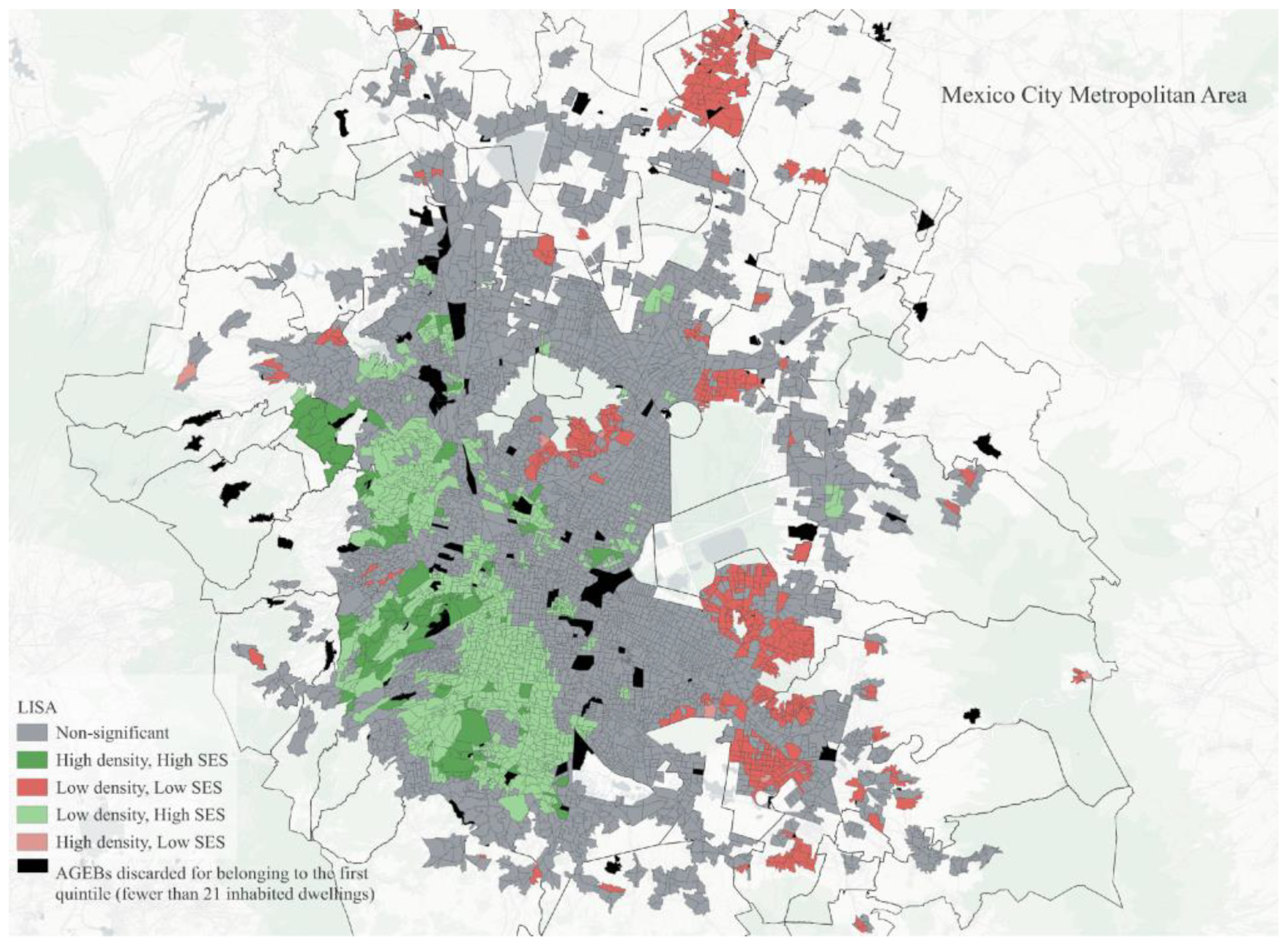
Figure A2.
LISA Analysis of Spatial Correlation of the Metropolitan Area of Monterrey, Considering the Density of Public Spaces for PA and the AMAI Socioeconomic Status Values by AGEB.
Figure A2.
LISA Analysis of Spatial Correlation of the Metropolitan Area of Monterrey, Considering the Density of Public Spaces for PA and the AMAI Socioeconomic Status Values by AGEB.
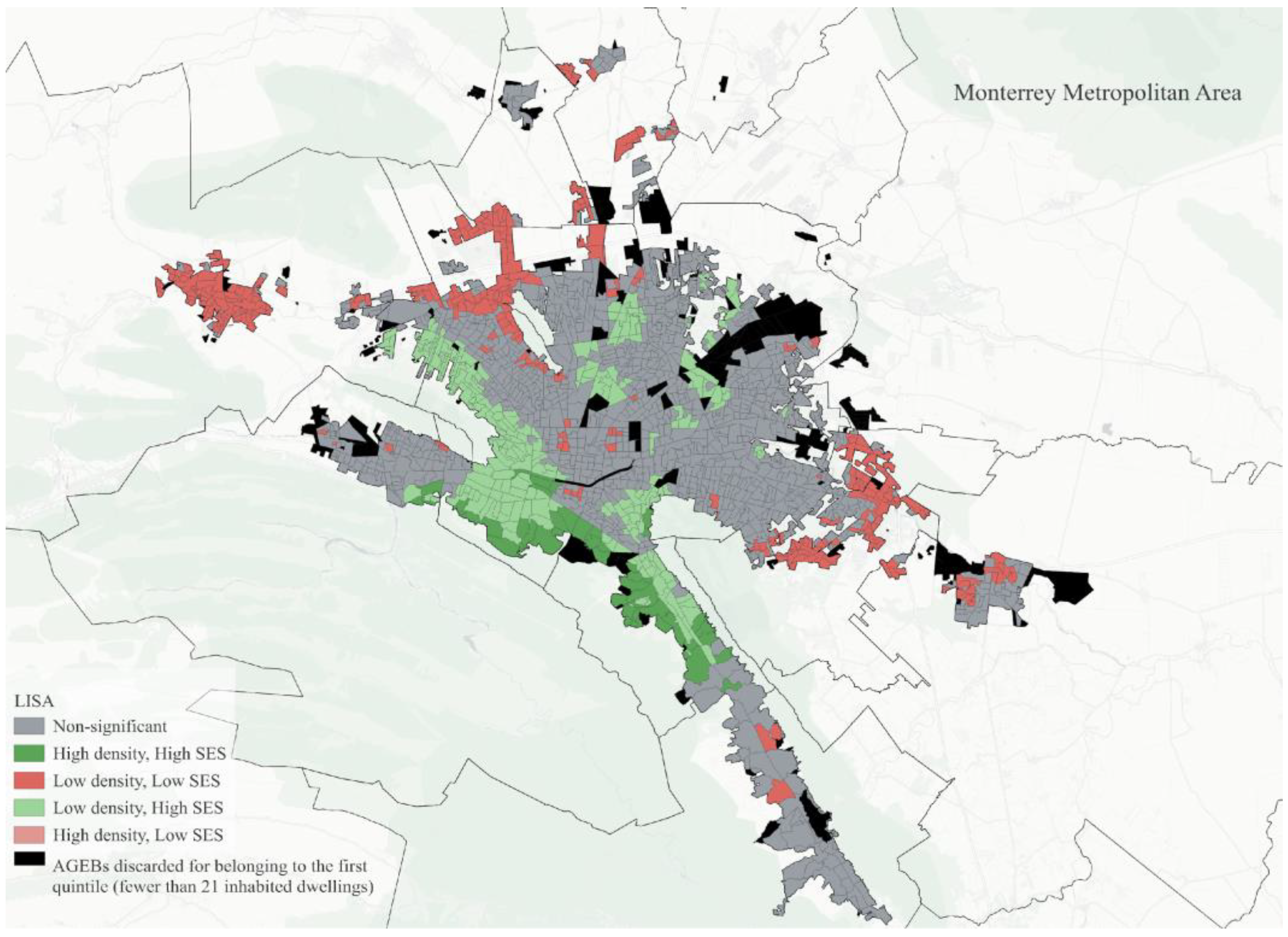
Figure A3.
LISA Analysis of Spatial Correlation of the Metropolitan Area of Guadalajara, Considering the Density of Public spaces for PA and the AMAI Socioeconomic Status Values by AGEB.
Figure A3.
LISA Analysis of Spatial Correlation of the Metropolitan Area of Guadalajara, Considering the Density of Public spaces for PA and the AMAI Socioeconomic Status Values by AGEB.
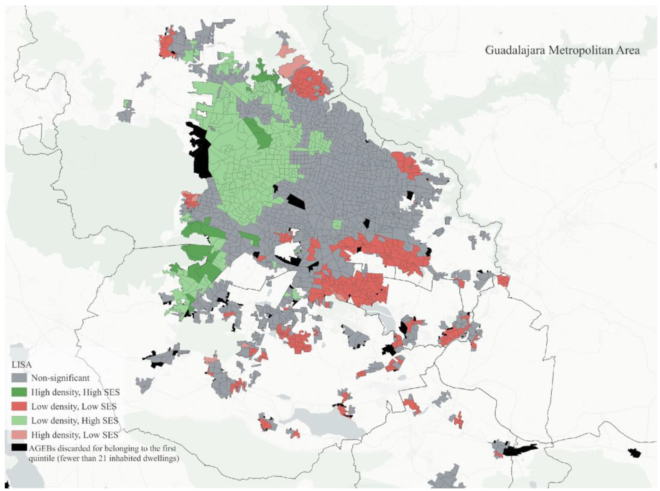
Table A1, Table A2 and Table A3 show the descriptive statistics (mean, standard deviation, minimum and maximum value) of the clusters derived from the LISA spatial correlation analysis, with the CONAPO database and the distribution of spaces for physical activity.

Table A1.
Marginalization Index by LISA cluster: Metropolitan Area of Mexico City.
| Marginalization index | |||||
| LISA Cluster | Observations | Mean | Standard deviation | Minimum | Maximum |
| Non- Significant AGEBs |
6,080 | 121.5 | 2.3 | 99.6 | 127.5 |
| High Density, Low Marginalization | 132 | 124.3 | 1.8 | 115.0 | 128 |
| Low Density, High Marginalization | 728 | 117.1 | 3.1 | 99.7 | 125 |
| Low Density, Low Marginalization | 1,112 | 123.8 | 1.3 | 116.7 | 127.6 |
| High Density, High Marginalization | 8 | 115.6 | 3.6 | 109 | 119.8 |
Source: Prepared by the authors. Note: The denominations shown in the high/low marginalization symbology are derived from the low/high marginalization index levels, respectively.
Table A2.
Marginalization Index by LISA cluster: Monterrey Metropolitan Area.
| Marginalization index | |||||
| LISA Cluster | Observations | Mean | Standard deviation | Minimum | Maximum |
| Non- Significant AGEBs |
1,278 | 123.2 | 2 | 99.6 | 127.5 |
| High Density, Low Marginalization | 23 | 126.4 | 1.2 | 121.9 | 127.5 |
| Low Density, High Marginalization | 236 | 120.5 | 2.3 | 109.4 | 126.7 |
| Low Density, Low Marginalization | 315 | 125.4 | 2.3 | 90.3 | 127.6 |
| High Density, High Marginalization | 8 | 122.1 | 3.2 | 118.3 | 126.9 |
Source: Prepared by the authors. Note: The denominations shown in the high/low marginalization symbology are derived from the low/high marginalization index levels respectively.
Table A3.
Marginalization Index by LISA cluster: Guadalajara Metropolitan Area.
| Marginalization Index | |||||
| LISA Cluster | Observations | Mean | Standard deviation | Minimum | Maximum |
| Non- Significant AGEBs |
1,236 | 121.2 | 2.5 | 102.6 | 126.9 |
| High Density, Low Marginalization | 24 | 124.1 | 2.7 | 117.3 | 127.6 |
| Low Density, High Marginalization | 200 | 117.3 | 2.9 | 106.3 | 124.8 |
| Low Density, Low Marginalization | 347 | 124.4 | 1.5 | 115.1 | 127.4 |
| High Density, High Marginalization | 8 | 115.8 | 5.6 | 107.1 | 126 |
Source: Prepared by the authors. Note: The denominations shown in the high/low marginalization symbology result from the low/high marginalization index levels, respectively.
References
- Cleven, L.; Krell-Roesch, J.; Nigg, C.R.; Woll, A. The association between physical activity with incident obesity, coronary heart disease, diabetes and hypertension in adults: A systematic review of longitudinal studies published after 2012. BMC Public Health 2020, 20, 1–15. [CrossRef]
- Yang, Y.; Mao, X.; Li, W.; Wang, B.; Fan, L. A meta-analysis of the effect of physical activity programs on fundamental movement skills in 3–7-year-old children. Front. Public Health 2025, 12, (artículo 1489141). [CrossRef]
- Shan, R.; Shao, S.; Li, L.; Zhang, D.; Chen, J.; Xiao, W.; Zhang, X.; Liu, Z. Mindfulness-based interventions for improvement of lifestyle behaviors and body mass index in children with overweight or obesity: A systematic review and meta-analysis. Eur. J. Pediatr. 2025, 184, 132. [CrossRef]
- Ding, D.; Sallis, J.; Kerr, J.; Lee, S.; Rosenberg, D.E. Neighborhood environment and physical activity among youth: A review. Am. J. Prev. Med. 2011, 41, 442–455. [CrossRef]
- Gemmell, E.; Ramsden, R.; Brussoni, M.; Brauer, M. Influence of neighborhood built environments on the outdoor free play of young children: A systematic, mixed-studies review and thematic synthesis. J. Urban Health 2023, 100, 118–150. [CrossRef]
- Humpel, N.; Owen, N.; Leslie, E. Environmental factors associated with adults’ participation in physical activity: A review. Am. J. Prev. Med. 2002, 22, 188–199. [CrossRef]
- Giles-Corti, B.; Vernez-Moudon, A.; Reis, R.; et al. City planning and population health: A global challenge. Lancet 2016, 388, 2912–2924. [CrossRef]
- UN-Habitat. World Cities Report 2022: Envisaging the Future of Cities; UN-Habitat: Nairobi, Kenya, 2022. Available online: https://unhabitat.org/sites/default/files/2022/06/wcr_2022.pdf (accessed on 1 July 2025).
- Ojeda-Revah, L. Equidad en el acceso a las áreas verdes urbanas en México: Revisión de literatura. Soc. Ambient. 2020, 24, 1–28. [CrossRef]
- Casillas Zapata, A.M. Desigualdad en la dotación de áreas verdes en el municipio de Monterrey: Una injusticia ambiental. Región Soc. 2023, 35, 1–24. [CrossRef]
- Higgs, C.; Badland, H.; Simons, K.; Knibbs, L.; Giles-Corti, B. The Urban Liveability Index: Developing a policy-relevant urban liveability composite measure and evaluating associations with transport mode choice. Int. J. Health Geogr. 2019, 18, 14. [CrossRef]
- Adler, N.E.; Boyce, T.; Chesney, M.; Cohen, S.; Folkman, S.; Kahn, R.L.; Syme, S.L. Socioeconomic status and health: The challenge of the gradient. Am. Psychol. 1994, 49, 15–24. [CrossRef]
- Mayen Huerta, C. Rethinking the distribution of urban green spaces in Mexico City: Lessons from the COVID-19 outbreak. Urban For. Urban Green. 2022, 70, (artículo). (Sin DOI informado).
- Núñez, J. Análisis espacial de las áreas verdes urbanas de la Ciudad de México. Econ. Soc. Territ. 2021, 21, 803–833. [CrossRef]
- Fernández-Álvarez, R. Distribución inequitativa del espacio público verde en la Ciudad de México: Un caso de injusticia ambiental. Econ. Soc. Territ. 2017, 399–428. [CrossRef]
- SEDATU. Metrópolis de México 2020; SEDATU: Ciudad de México, México, 2020. Available online: https://www.gob.mx/cms/uploads/sedatu/MM2020_06022024.pdf (accessed on 1 July 2025).
- Wolch, J.R.; Byrne, J.; Newell, J.P. Urban green space, public health, and environmental justice: The challenge of making cities ‘just green enough’. Landsc. Urban Plan. 2014, 125, 234–244. [CrossRef]
- INEGI. Geografía y Medio Ambiente; INEGI: Ciudad de México, México, 2020. Available online: https://www.inegi.org.mx/temas/mg/ (accessed on 1 July 2025).
- INEGI. Información Demográfica y Social; INEGI: Ciudad de México, México, 2020. Available online: https://www.inegi.org.mx/programas/ccpv/2020/#tabulados (accessed on 1 July 2025).
- Consejo Nacional de Población. Índices de Marginación 2020; Gobierno de México: Ciudad de México, México, 2021. Available online: https://www.gob.mx/conapo/documentos/indices-de-marginacion-2020-284372 (accessed on 1 July 2025).
- Anselin, L. GeoDa (1.22); The University of Chicago Campaign: Chicago, IL, USA, 2003. Available online: https://geodacenter.github.io/ (accessed on 3 July 2025).
- Celemín, J.P. Autocorrelación espacial e indicadores locales de asociación espacial: Importancia, estructura y aplicación. Rev. Univ. Geogr. 2009, 18, 11–31.
- Fuentes, N.A. Crecimiento económico y desigualdades regionales en México: El impacto de la infraestructura. Región Soc. 2003, 15, 81–106.
- Asociación Mexicana de Agencias de Inteligencia de Mercado y Opinión (AMAI). Niveles Socioeconómicos (NSE); AMAI: Ciudad de México, México. Available online: https://www.amai.org/NSE/index.php (accessed on 1 July 2025).
- Sallis, J.; Floyd, M.; Rodríguez, D.; Saelens, B. Role of built environments in physical activity, obesity, and cardiovascular disease. Circulation 2012, 125, 729–737. [CrossRef]
- Ortiz, C. Writing the Latin American City: Trajectories of urban scholarship. Urban Stud. 2023, 61, 399–425. (Original work published 2024). [CrossRef]
- Gómez-Baggethun, E.; Barton, D. Classifying and valuing ecosystem services for urban planning. Ecol. Econ. 2013, 86, 235–245. [CrossRef]
- Barton, H.; Grant, M. Urban planning for healthy cities: A review of the progress of the European Healthy Cities Programme. J. Urban Health 2012, 89, 129–131. [CrossRef]
- Heath, G.W.; Parra, D.C.; Sarmiento, O.L.; Andersen, L.B.; Owen, N.; Goenka, S.; Montes, F.; Brownson, R.C.; Lancet Physical Activity Series Working Group. Evidence-based intervention in physical activity: Lessons from around the world. Lancet 2012, 380, 272–281. PMID: 22818939. [CrossRef]
- Braveman, P.A.; Cubbin, C.; Egerter, S.; et al. Socioeconomic status in health research: One size does not fit all. JAMA 2005, 294, 2879–2888 (accessed on 1 July 2025). [CrossRef]
Figure 1.
Global Spatial Association between Marginalization Index and Density of PA Spaces. Source: Prepared by the authors.
Figure 1.
Global Spatial Association between Marginalization Index and Density of PA Spaces. Source: Prepared by the authors.
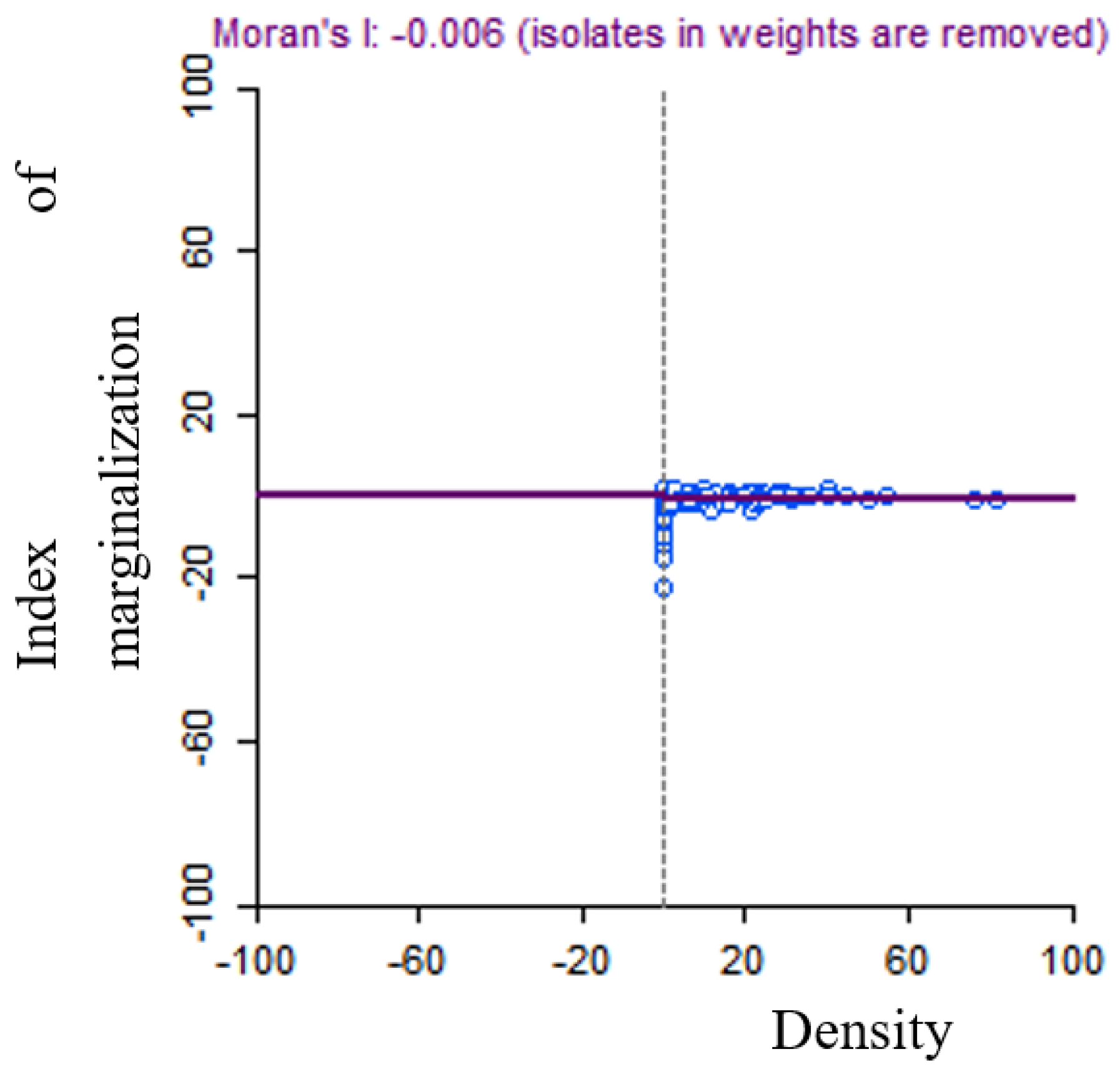
Figure 2.
Distribution of Public Spaces for PA in the Mexico City MA. Source: Prepared by the authors.
Figure 2.
Distribution of Public Spaces for PA in the Mexico City MA. Source: Prepared by the authors.
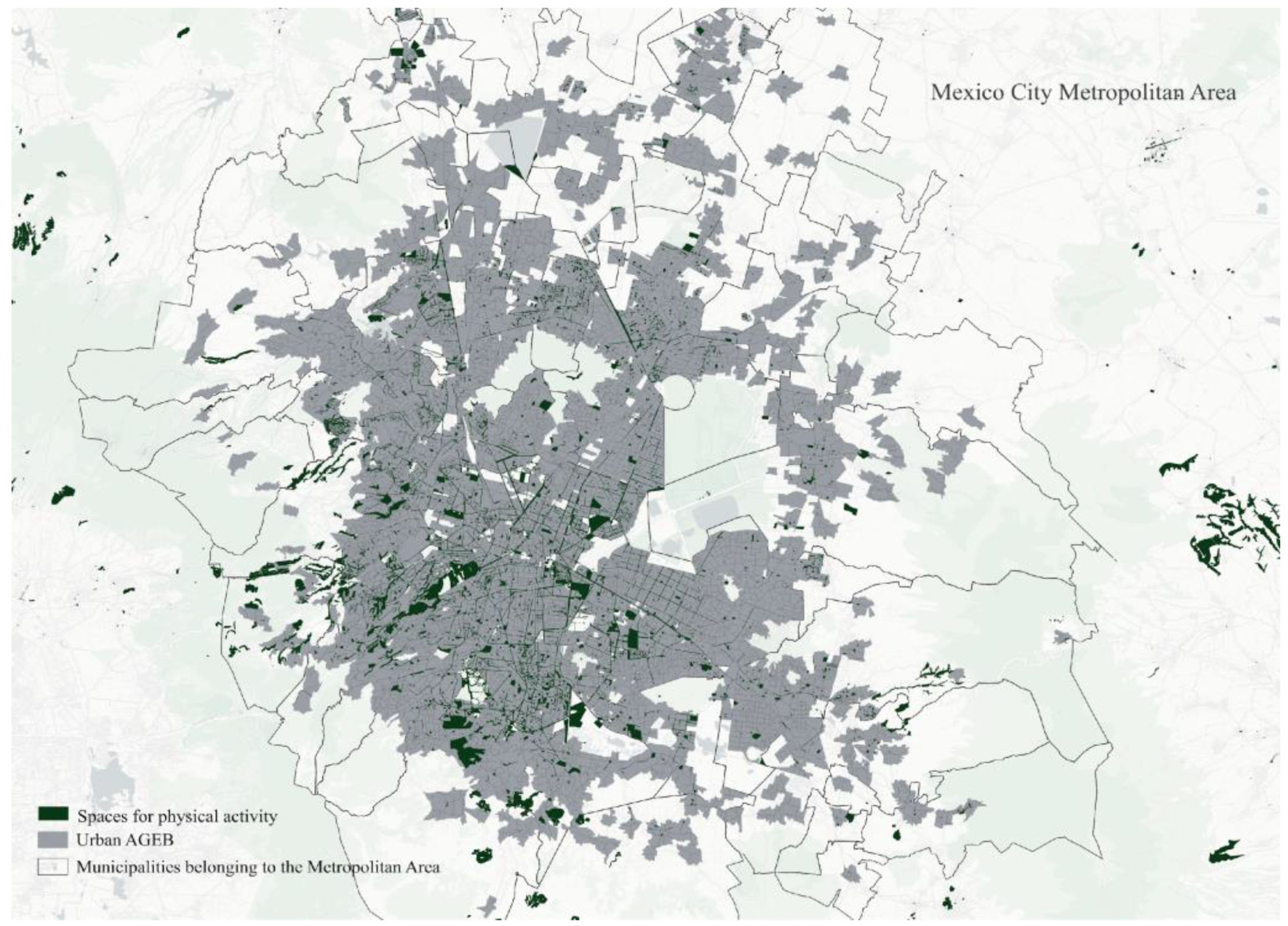
Figure 3.
Distribution of Public Spaces for PA in the Monterrey MA. Source: Prepared by the authors.
Figure 3.
Distribution of Public Spaces for PA in the Monterrey MA. Source: Prepared by the authors.
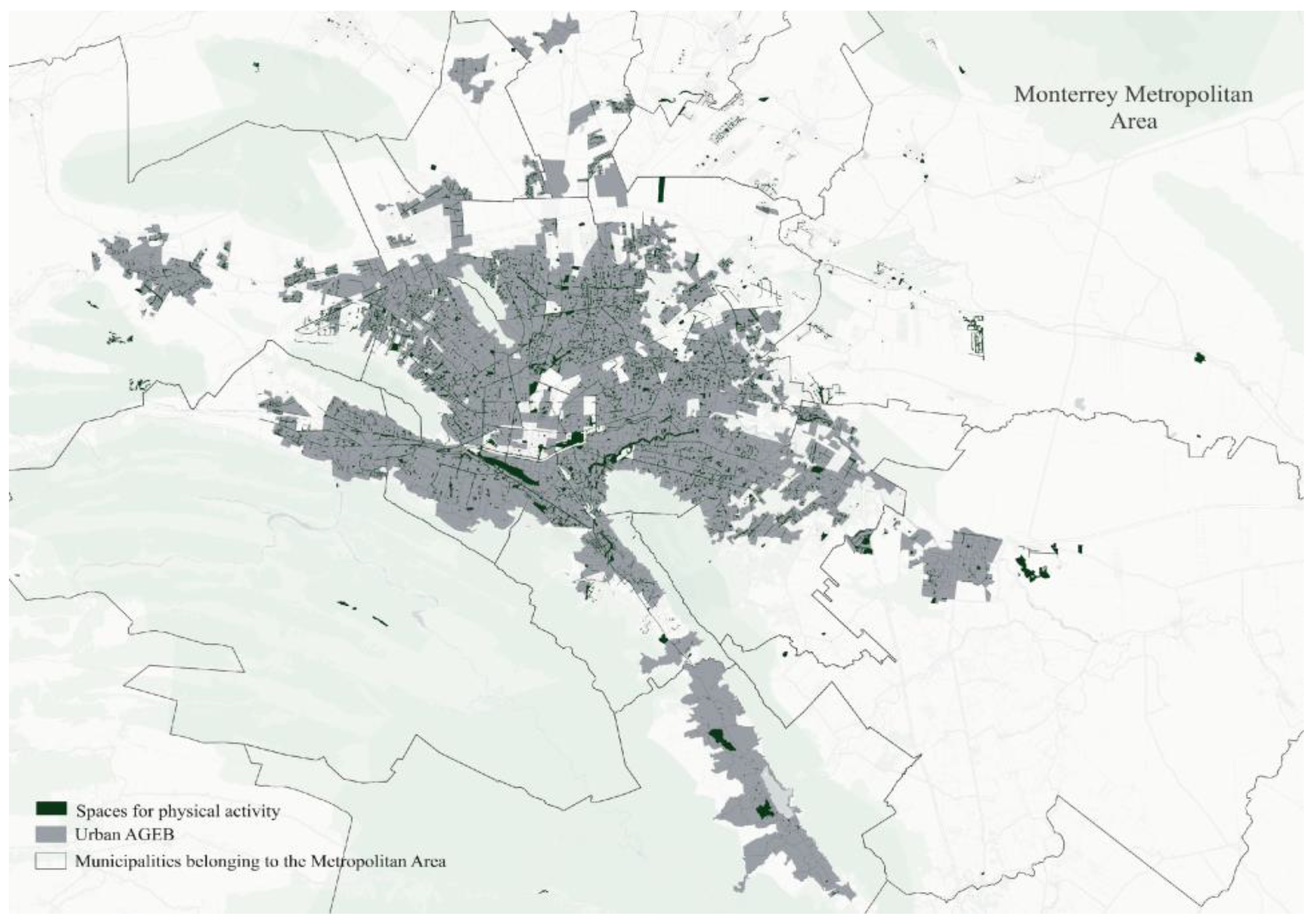
Figure 4.
Distribution of Public Spaces for PA in the Guadalajara MA. Source: Prepared by the authors.
Figure 4.
Distribution of Public Spaces for PA in the Guadalajara MA. Source: Prepared by the authors.
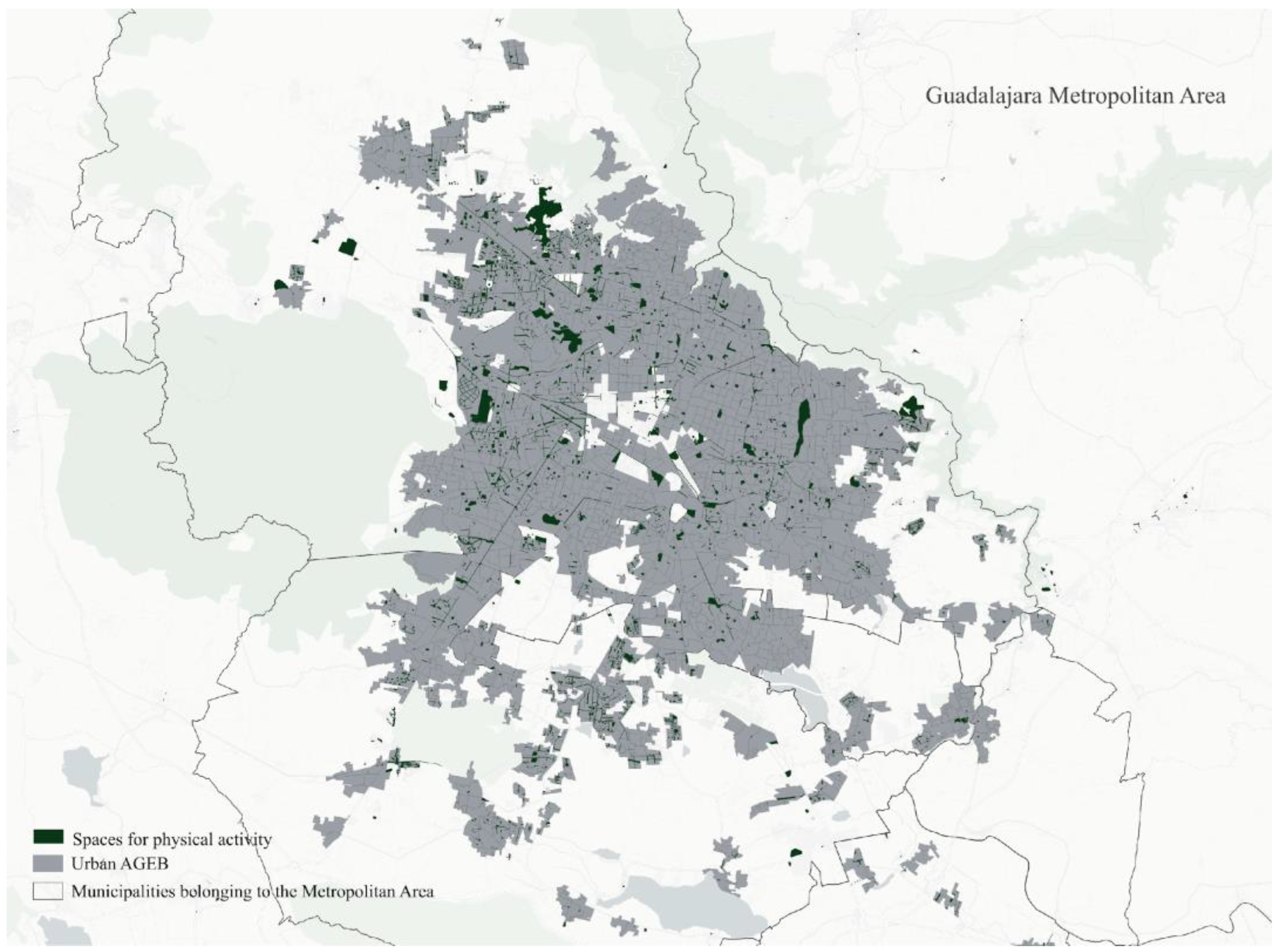
Figure 5.
LISA Analysis of the Spatial Association of the Density of Public Spaces for PA and the Marginalization Index in AGEBs in the Mexico City Metropolitan Area. Source: Prepared by the authors. Note: The denominations shown in the high/low marginalization symbology reflect the low/high marginalization index levels respectively.
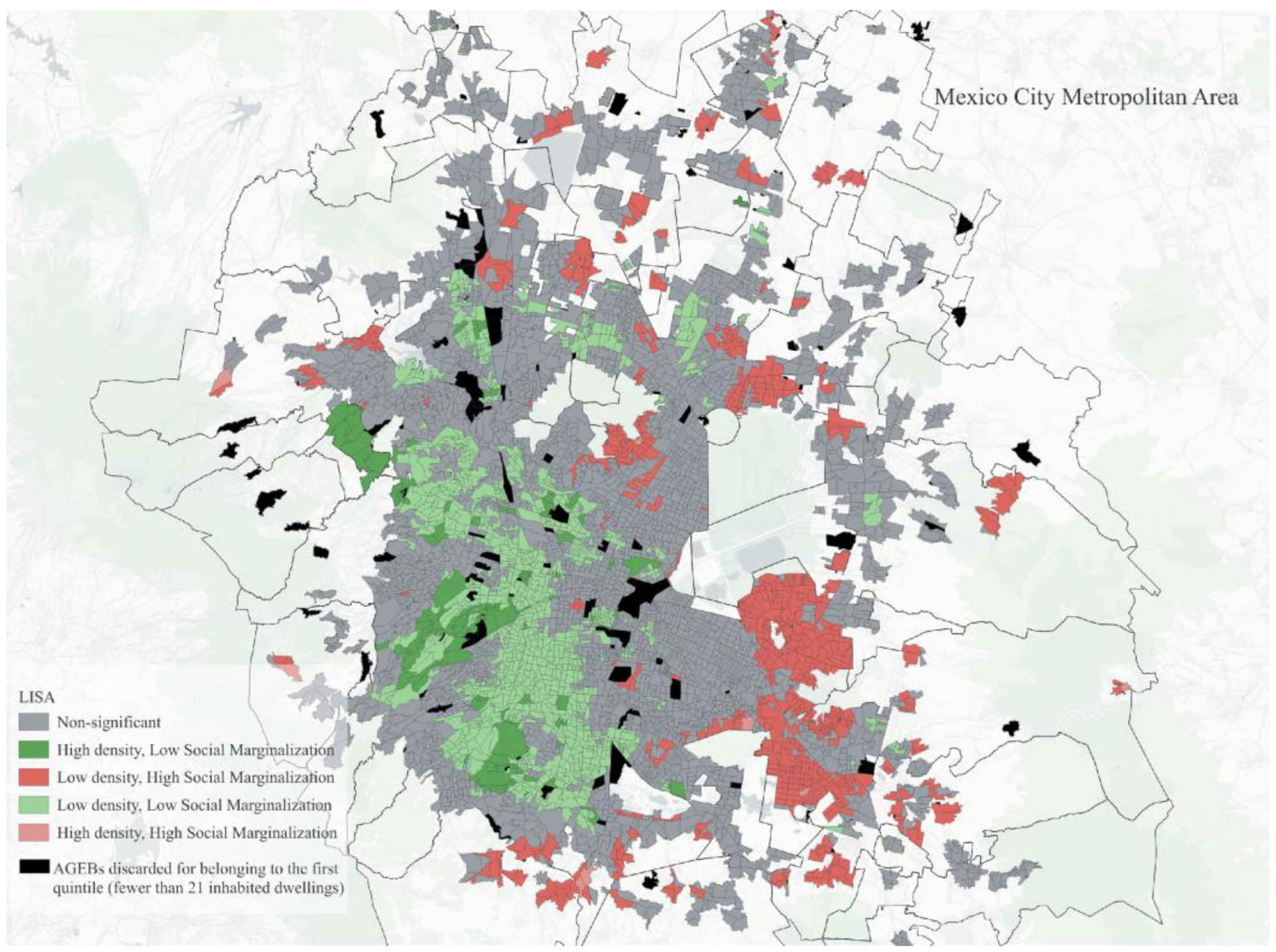
Figure 6.
LISA Analysis of the Spatial Association of the Density of Public Spaces for PA and the Marginalization Index in AGEBs in the Monterrey Metropolitan Area. Source: Prepared by the authors. Note: The denominations shown in the high/low marginalization symbology are derived from the low/high marginalization index levels, respectively.
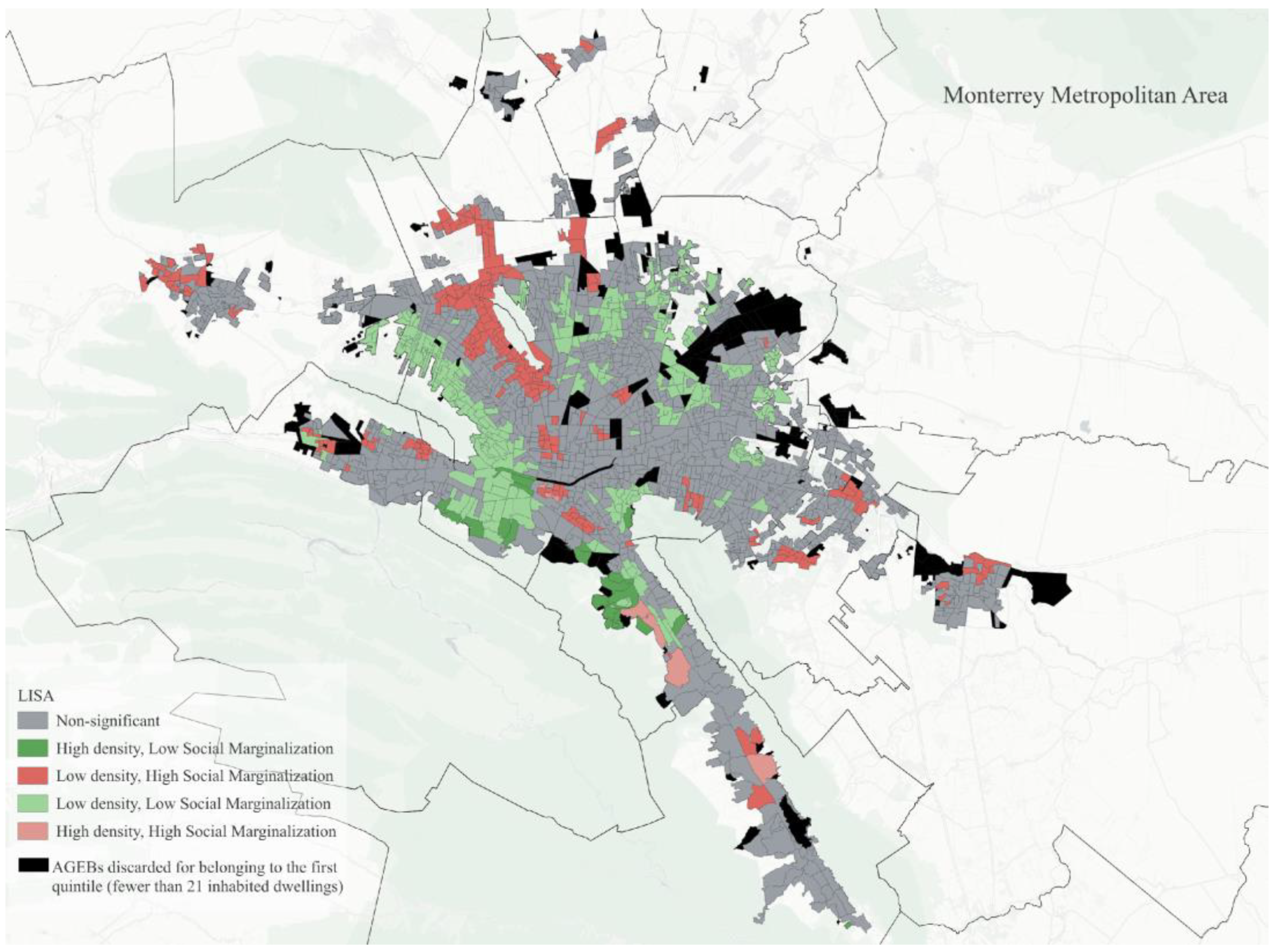
Figure 7.
LISA Analysis of the Spatial Association of the Density of Public Spaces for PA and the Marginalization Index of AGEBs in the Guadalajara Metropolitan Area. Source: Prepared by the authors. Note: The denominations shown in the high/low marginalization symbology reflect the low/high marginalization index levels respectively.
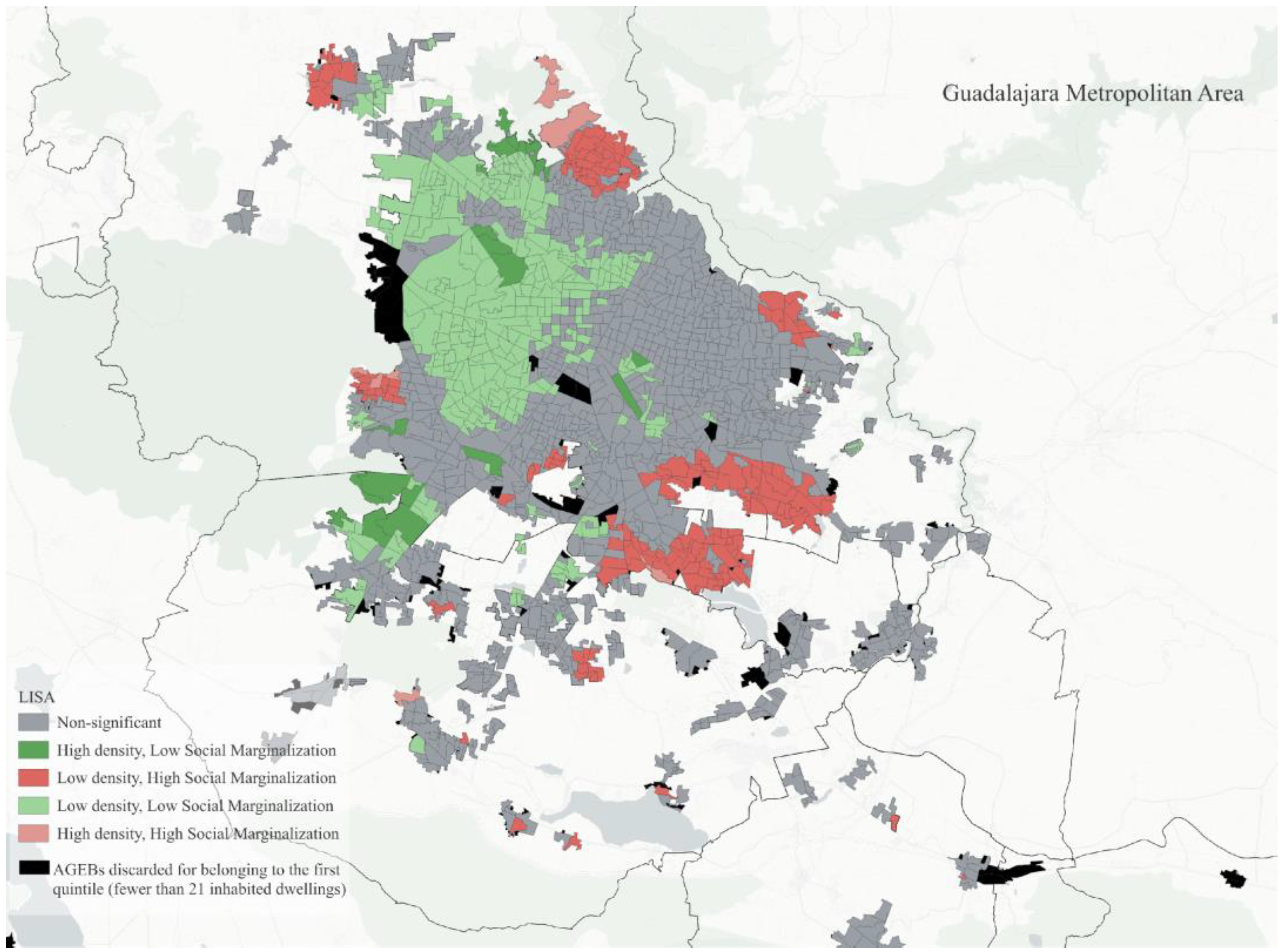
Table 1.
Marginalization Index, Density of Green Areas and Number of Inhabited Dwellings in AGEBs (n = 50,372).
Table 1.
Marginalization Index, Density of Green Areas and Number of Inhabited Dwellings in AGEBs (n = 50,372).
| Variable | Mean | Standard deviation | Minimum | Maximum |
| Inhabited dwellings | 559.3 | 513.4 | 22 | 9,008 |
| Marginalization index | 120.0 | 5.4 | 53.4 | 128.0 |
| Space density for PA | 15,332 | 277,425 | 0 | 22,700,000 |
Source: Prepared by the authors using data from CONAPO 2020, INEGI 2020, and OSM.
Table 2.
Frequency of AGEBs by Classification Category according to the LISA Analysis and Quintile of the Marginalization Index.
Table 2.
Frequency of AGEBs by Classification Category according to the LISA Analysis and Quintile of the Marginalization Index.
| Marginalization Index | |||||
| LISA Cluster | Observations | Mean | Standard deviation | Minimum | Maximum |
| Non-significant | 34,368 | 119.8 | 3.8 | 62.6 | 127.5 |
| High Density, Low Marginalization | 441 | 123.2 | 10.6 | 90.3 | 128 |
| Low Density, High Marginalization | 4,240 | 112.3 | 9.2 | 61.2 | 126.3 |
| Low Density, Low Marginalization | 10,142 | 124 | 2.2 | 78.4 | 127.6 |
| High Density, High Marginalization | 78 | 112.7 | 8.0 | 65 | 126.9 |
Source: Prepared by the authors based on the results of the LISA analysis. Note: The non-significant LISA cluster indicates that there is insufficient statistical evidence to assume a spatial correlation between the value of the density of spaces for physical activity in an AGEB and their marginalization index The denominations shown in the high/low marginalization symbology reflect the low/high marginalization index levels respectively.
Table 3.
Density of Public Spaces for PA by Classification in the LISA Analysis.
| Density of Spaces for Physical Activity | |||||
| LISA Cluster | Observations | Mean | Standard deviation | Minimum | Maximum |
| Non-significant | 34,368 | 15,035.2 | 298,302.6 | 0 | 22,700,000 |
| High Density, Low Marginalization | 441 | 308,689.7 | 993,634.3 | 15,030.4 | 11,300,000 |
| Low Density, High Marginalization | 4,240 | 254.4 | 1,148.2 | 0 | 14,169.8 |
| Low Density, Low Marginalization | 10,142 | 1,113.1 | 2,061.4 | 0 | 14,979.4 |
| High Density, High Marginalization | 78 | 945,382.3 | 1,650,180 | 16,104.7 | 6,615,306 |
Source: Prepared by the authors. Note: The denominations shown in the high/low marginalization symbology reflect the low/high marginalization index levels respectively.
Table 4.
Marginalization Index, Density of Green Areas and Number of Inhabited Dwellings in Urban AGEBs (n = 50,372) in the Metropolitan Areas.
Table 4.
Marginalization Index, Density of Green Areas and Number of Inhabited Dwellings in Urban AGEBs (n = 50,372) in the Metropolitan Areas.
| Mexico City Metropolitan Area | |||||
| Variable | Observations | Mean | Standard deviation | Minimum | Maximum |
| Density of green areas | 9,285 | 21,642.4 | 285,519.3 | 0 | 11,300,000 |
| Marginalization index | 9,275 | 121.6 | 3 | 90.3 | 128 |
| Inhabited dwellings | 9,285 | 951.3 | 679.4 | 22 | 9008 |
| Guadalajara Metropolitan Area | |||||
| Density of green areas | 1,830 | 18,072.2 | 244,019.9 | 0 | 6,798,192 |
| Marginalization index | 1,824 | 121.4 | 3.1 | 102.6 | 127.6 |
| Inhabited dwellings | 1,830 | 779.6 | 537.7 | 22 | 4,098 |
| Monterrey Metropolitan Area | |||||
| Density of green areas | 1,879 | 68,092.2 | 567,505.5 | 0 | 11,300,000 |
| Marginalization index | 1,876 | 123.3 | 2.5 | 90.3 | 127.6 |
| Inhabited dwellings | 1,879 | 750.6 | 464.2 | 22 | 3,253 |
Table 5.
Means and Medians of the Density of Spaces for PA according to the Marginalization Quartiles in the AGEBs of the Three Largest Metropolitan Areas.
Table 5.
Means and Medians of the Density of Spaces for PA according to the Marginalization Quartiles in the AGEBs of the Three Largest Metropolitan Areas.
| Q1 | Q2 | Q3 | Q4 | P | |
| Three metropolitan areas | |||||
| Mean | 14,834.5 | 9,031.0 | 13,411.9 | 42,469.8 | <0.000 |
| Median | 0.0 | 108.8 | 287.8 | 757.7 | <0.000 |
| Mexico City Metropolitan Area | |||||
| Mean | 3,153.0 | 2,611.0 | 5,650.5 | 17,243.5 | <0.000 |
| Median | 0 | 60.6 | 189.7 | 563.8 | <0.000 |
| Guadalajara Metropolitan Area | |||||
| Mean | 27,161.2 | 4,523.9 | 5,306.0 | 35,186.3 | 0.138 |
| Median | 0 | 33.1 | 184.2 | 693.5 | <0.000 |
| Monterrey Metropolitan Area | |||||
| Mean | 37,594.9 | 32,481.6 | 44,378.6 | 124,423.7 | 0.021 |
| Median | 257.6 | 431.5 | 675.6 | 1,356.3 | <0.000 |
P values were obtained using ANOVA (to compare means) and the Kruskal-Wallis test was used to compare medians.
Disclaimer/Publisher’s Note: The statements, opinions and data contained in all publications are solely those of the individual author(s) and contributor(s) and not of MDPI and/or the editor(s). MDPI and/or the editor(s) disclaim responsibility for any injury to people or property resulting from any ideas, methods, instructions or products referred to in the content. |
© 2025 by the authors. Licensee MDPI, Basel, Switzerland. This article is an open access article distributed under the terms and conditions of the Creative Commons Attribution (CC BY) license (http://creativecommons.org/licenses/by/4.0/).
Copyright: This open access article is published under a Creative Commons CC BY 4.0 license, which permit the free download, distribution, and reuse, provided that the author and preprint are cited in any reuse.


