Submitted:
07 October 2025
Posted:
08 October 2025
You are already at the latest version
Abstract
Forecasting traffic flow is vital for optimizing resource allocation and improving urban traffic management efficiency. However, most existing traffic forecasting methods primarily emphasize road node connectivity when modelling spatial dependencies, often overlooking the impact of node transmission characteristics and inter-node distances on spatial feature propagation. This limitation restricts capturing temporal dynamics in spatial dependencies within traffic flow. To address this challenge, this study proposes a Transfer-aware Spatio-Temporal Graph Attention Network with Long-Short Term Memory and Transformer module (TAGAT-LSTM-trans). The model constructs a transfer probability matrix to represent each node’s ability to transmit traffic characteristics and introduces a distance decay matrix to replace the traditional adjacency matrix, thereby offering a more accurate representation of spatial dependencies between nodes. Our proposed model integrates a Graph Attention Network (GAT) to build a TA-GAT module for capturing spatial features, while a gating network dynamically aggregates information across adjacent time steps. Temporal dependencies are modelled using LSTM and a Transformer encoder, with fully connected layers ensuring precise forecasts. Experiments on real-world highway datasets show that TAGAT-LSTM-trans outperforms baseline models in spatio-temporal dependency modelling and traffic flow forecasting accuracy.
Keywords:
graph attention network
; traffic flow prediction
; long-short term memory model
; transformer
1. Introduction
Traffic flow prediction is a fundamental problem in spatiotemporal data forecasting [1]. In the temporal dimension, traffic flow exhibits dynamic variations, primarily characterized by proximity and periodicity [2]. Proximity suggests that traffic flows occurring within short time intervals tend to exhibit stronger correlations, while periodicity reflects recurring traffic patterns over regular time intervals. In the spatial dimension, the topological structure of the road network influences the spatial distribution of traffic flow [3]. For example, traffic on a given road is affected by directly connected roads, spatially unconnected roads can also impact traffic flow through diffusion effects. Various factors jointly shape the spatiotemporal characteristics of traffic flow. For instance, working hours on weekdays result in a significant increase in traffic during the morning and a marked decrease in the evening, whereas this pattern differs on weekends [4]. Moreover, the congestion level of a particular road affects the traffic patterns of neighbouring roads, and as congestion intensifies and distance increases, the road’s influence on surrounding roads gradually diminishes.
The spatial characteristics of traffic flow also exhibit temporal continuity. As illustrated in Figure 1, the traffic state at a node is affected by its neighbouring nodes and historical traffic conditions. This temporal dependency underscores the important role of historical traffic conditions on future traffic state. Therefore, developing a model that effectively captures the spatio-temporal features of traffic is essential for precise prediction.
Deep learning models have become the dominant approach in traffic flow prediction, with Graph Convolutional Networks (GCNs) and Graph Attention Network (GAT) proving effective in capturing the spatial dependencies of traffic flow. However, these models face challenges when dealing with complex road networks and dynamic temporal changes. For instance, GCNs operate under the assumption that all nodes are equally important, while GAT employ a multi-head self-attention (MSA) mechanism to assign varying weights, improving prediction accuracy. Despite these advancements, GAT lacks interpretability and does not account for the transmission capabilities of nodes' traffic features. Additionally, most models separate spatial and temporal feature extraction, overlooking temporal dynamics within spatial features and neglecting spatiotemporal continuity. Moreover, sequence models like Long-Short Term Memory (LSTM) suffer from information decay in long temporal sequences, limiting their capacity to capture global features.
In response to these limitations, we propose the Transfer-aware Spatio-Temporal Graph Attention Network with Long-Short Term Memory and Transformer (TAGAT-LSTM-trans). TAGAT-LSTM-trans consists of three core modules: the TA-GAT module captures spatial dependencies; the gating network module performs preliminary temporal aggregation by weighting and merging features from adjacent time steps, thereby enhancing spatial feature representation; and the LSTM network, combined with a simplified Transformer Encoder module, further models both local and global temporal features. This integration enables TAGAT-LSTM-trans to learn intricate spatiotemporal dependencies, improving the precision of traffic flow forecasting. The primary contributions of this research are as follows:
- (1)
- TAGAT-LSTM-trans mitigates the shortcomings of GAT in capturing road spatial features by introducing a transfer probability matrix, which represents the ability of road nodes to transmit and receive traffic flow features based on their current state. Additionally, a distance decay matrix captures the diminishing spatial dependencies between nodes as distance increases. By integrating these matrices into GAT, the model more effectively extracts spatial features in road networks.
- (2)
- TAGAT-LSTM-trans incorporates a gating network layer to bridge spatial and temporal feature extraction. This structure enables the model to dynamically integrate spatial features from different time intervals, capturing temporal dynamics and enhancing its capability to model complex traffic patterns.
- (3)
- TAGAT-LSTM-trans combines LSTM with a Transformer Encoder module, leveraging the Transformer's strong global feature extraction capabilities and LSTM's proficiency in handling extended temporal sequences. This fusion allows the model to detect local and global temporal variations, resulting in more detailed and comprehensive traffic flow features.
This paper is organized as follows: Section 2 reviews foundational concepts and recent advancements in traffic flow forecasting. Section 3 details the architecture and methodology of the proposed TAGAT-LSTM-trans model. Section 4 presents the experimental results and discusses the findings. Section 5 concludes the study and proposes potential research directions.
2. Related work
Deep learning technologies have revolutionized traffic flow prediction, with Convolutional Neural Networks (CNNs) and Recurrent Neural Networks (RNNs) showing significant advantages in capturing spatio-temporal characteristics. Studies demonstrate that CNNs are particularly effective at extracting spatial features, leading to improved prediction accuracy [5,6,7]. For instance, Zhang et al. [8] utilized a Spatio-Temporal Feature Selection Algorithm (STFSA) to convert traffic characteristics into two-dimensional matrices to enhance the input for CNNs, thereby improving prediction performance. RNNs and LSTM are widely applied for learning the temporal characteristics of traffic flow owing to their excellent performance in modelling sequential characteristics and long-term dependencies [9,10]. However, traditional CNNs and RNNs focus predominantly on temporal or spatial features, failing to fully exploit the spatio-temporal correlations in traffic flow data. Researchers have increasingly combined different neural networks into hybrid models to overcome these limitations. As an illustration, Narmadha and Vijayakumar [11] proposed a hybrid model combining CNNs and LSTM for traffic flow forecasting, showing improved accuracy compared to traditional models. However, these algorithms primarily focus on Euclidean data, such as 2D images and regular grids, they struggle with road networks, which possess non-Euclidean characteristics. This limitation renders CNNs inadequate for effectively capturing the complex topology of these networks.
GCNs have proven particularly effective in modelling non-Euclidean data, making them increasingly popular for spatial modelling in road networks [12,13,14]. GCNs construct adjacency matrices to aggregate features from neighbouring nodes but assume that all nodes are equally important. In contrast, GAT introduces an MSA mechanism to assign weights to nodes dynamically, enabling more nuanced modelling of spatial relationships [15]. For instance, Zhang et al. [16] developed a Spatio-temporal Graph Attention Network (STGAT) that utilizes GAT for spatial dependencies and LSTM for temporal features, improving prediction accuracy and robustness. Li and Lasenby [17] enhanced prediction precision by incorporating speed, volume, and weather information into a GAT and LSTM hybrid model. However, RNNs and LSTM, being sequential processing models, often struggle with capturing long-range dependencies due to their reliance on previous time step calculations, which can degrade performance over longer sequences. By leveraging MSA mechanisms, the Transformer model proves to be more effective in modelling these dependencies, making it an essential tool for traffic flow forecasting. Reza et al. [18] demonstrated that an MSA Transformer model outperforms RNNs and LSTM in long-term traffic flow forecasting.
Recent studies have focused on refining the extraction and fitting of spatio-temporal features to capture more complex traffic characteristics, often employing various deep-learning fusion models to improve prediction accuracy. For instance, Chen et al. [19] developed a bidirectional Transformer model (Bi-STAT) that utilizes a memory decoder to provide additional auxiliary information for prediction tasks. Ji et al. [20] introduced a self-supervised learning framework for spatio-temporal data that enhances traffic pattern representation, effectively addressing temporal variations due to differing traffic conditions. Jiang et al. [21] developed the propagation delay-aware dynamic long-range transformer (PDFormer), a transformer model that captures spatial dependencies dynamically using MSA while modelling propagation delays in spatial information. Bao et al. [22] presented a Spatio-Temporal Complex Graph Convolutional Network (ST-CGCN), which improves the modelling of spatio-temporal features alongside external influences by integrating node correlations and external disturbances into a dynamic correlation matrix with self-learning weights.
Despite notable successes, these models continue to face several challenges. First, GAT assigns node weights based on the correlations of data features among traffic network nodes, adjusting these weights dynamically during training. While this mechanism improves prediction accuracy, it lacks interpretability. In real-world road networks, spatial dependencies are influenced not only by data feature correlations but also by current traffic states and inter-node distances, introducing additional complexity to the modelling of spatial relationships. Second, many existing models treat spatial and temporal feature extraction as independent processes. Although this separation has shown performance gains, it neglects the intrinsic continuity of spatial features in traffic flow, where spatial dependencies evolve in tandem with temporal dynamics. Moreover, LSTM's sequential processing nature often results in the degradation of hidden state information as the sequence length increases, limiting its capacity to capture global dependencies compared to attention-based models.
To address these limitations, we propose the TAGAT-LSTM-trans model. This model introduces a transmission probability matrix to represent the capacity of road nodes to transmit traffic features, replacing the traditional adjacency matrix with a distance decay matrix. This enhancement enables a more accurate representation of spatial dependencies and improves the performance of GAT. Additionally, the incorporation of a Gating Network allows the model better to capture the temporal continuity and variations of spatial features. Lastly, integrating the Transformer Encoder with LSTM leverages the strengths of both architectures, enhancing the extraction of both local and global temporal features and ultimately improving predictive accuracy.
3. Methods
The graph representation of the traffic network is constructed based on spatial connectivity and is denoted as : represents the set of all road nodes, here, denotes the overall number of nodes, and represents the set of edges. An edge exists between two nodes in if they are spatially connected. The adjacency matrix encodes the spatial connection of nodes: indicates a spatial link connecting nodes and , while otherwise, as in:
for each node in graph , the temporal characteristics are represented by , where denotes the historical traffic sequence length for each node, is the number of feature types available per node. In this paper, are considered. Thus, contains multiple feature values for each node over the time steps of history. Based on the above definitions, the traffic flow prediction problem can be formalized as:
where is the predicted traffic state matrix, with representing the prediction time step length. Here, denotes the model, which uses the historical traffic sequence along with the graph structure to forecast traffic over future time steps.
3.1. TAGAT-LSTM-Trans Deep Learning Framework
Traffic flow forecasting involves predicting spatio-temporal data, with the primary challenge being the effective modelling and extraction of both temporal and spatial features from traffic networks. Given these challenges, we designed a transfer-aware deep learning network model, TAGAT-LSTM-trans. The framework is illustrated in Figure 2 and comprises five key modules:
- (1)
- Inputs module: This module processes raw input data through smoothing and normalization, ensuring the data is properly preconditioned for subsequent modelling stages.
- (2)
- Spatial feature extraction module (TA-GAT): This module integrates a GAT, a transfer probability matrix, and a distance decay matrix. It is responsible for modelling and capturing the spatial dependencies within the road network, accounting for interactions between road nodes.
- (3)
- Gating Network module: Comprising multiple gating networks, this module performs preliminary temporal aggregation of the spatial features extracted by the TA-GAT module. It enhances the model's ability to capture temporal variations in spatial dependencies.
- (4)
- Temporal feature extraction module (LSTM-Trans): This module combines a Long-Short Term Memory (LSTM) network with a Transformer Encoder layer, effectively capturing temporal features in historical traffic sequences by modelling local and global temporal dynamics.
- (5)
- Training and output module: This module uses a fully connected (FC) layer to map the extracted spatio-temporal feature vectors to the prediction outcomes. The predicted results are then denormalized to revert them to their original scale. Finally, the model is trained using a loss function to optimize prediction accuracy.
3.2. Inputs Module
3.2.1. Smooth
Raw traffic data frequently contains substantial noise, often caused by sensor errors or exceptional events such as traffic accidents and road construction. This noise can considerably impair the model's training efficiency and prediction accuracy. Therefore, smoothing the raw data is an essential preprocessing step. Smoothing reduces short-term fluctuations, decreases the likelihood of model overfitting, and enhances overall model performance. In this study, we utilize a moving average filter to smooth the data and mitigate noise [23]. Given a time series data , the moving average filter is defined as follows:
where refers to the range of the moving window, denotes the raw data at the time step, and denotes the smoothed data after noise removal.
3.2.2. Normalization
Time series models are often influenced by statistical characteristics of data, such as the mean and standard deviation, potentially diminishing prediction accuracy. Therefore, normalization is another important data preprocessing step. A commonly used normalization method is Z-score normalization, which effectively eliminates dimensional differences between features by scaling the data to have a mean of 0 and a standard deviation of 1, conforming to a standard normal distribution. This transformation accelerates the convergence of gradient descent algorithms, ultimately improving model performance. For a given input data , the Z-score normalization is defined by:
where represents the mean of data, is the standard deviation, denotes the input data of feature , and is the normalized data.
3.3. Spatial Feature Extraction Module
3.3.1. GAT
The TA-GAT module extracts spatial features from traffic networks through three core components: the GAT, the transmission coefficient matrix, and the distance decay matrix.
In real-world traffic networks, the spatial relationships between road nodes and their neighbouring nodes are dynamic, varying over time in response to fluctuating traffic conditions. GAT introduces an MSA mechanism to capture these evolving relationships by assigning different weights to node connections, enabling a more efficient representation of spatial features within the traffic network. Specifically, the attention mechanism dynamically adjusts the influence of neighbouring nodes by identifying the most relevant spatial dependencies at each time step, enhancing the model's ability to capture temporal variability in spatial relationships. Our model uses an MSA mechanism in the GAT framework, enabling it to learn attention coefficients from multiple subspaces simultaneously, which results in richer and more comprehensive spatial representations. The architecture of the GAT model is depicted in Figure 3.
At every time step, GAT first defines a feature transformation matrix , which linearly transforms the input features of each node, thereby mapping them into a novel feature space, as shown:
where is the trainable feature transformation matrix, and denote the input features of node and the new features after transformation at layer , respectively.
Then, the attention mechanism calculates the weight between two connected nodes, denoted by:
where is attention vector, indicates the concatenation of feature vectors, and serves as the activation function to calculate the attention coefficient by merging the features of node and node , where is a neighbour of , and since may have multiple neighbours, it is necessary to perform normalization, as defined by:
where is the set of neighbours of node , and the attention weights are derived by applying normalization to the attention coefficients.
The output of node are calculated by using the attention weights to aggregate the features of its neighbouring nodes, which can be computed by:
where is an activation function, denotes the features of neighbouring nodes, is the attention weight of node relative to node . The new feature representation of node is obtained by aggregating the features from all neighbouring nodes.
The MSA mechanism strengthens the model's capacity to capture a wide range of feature information, significantly improving its performance [24]. By allowing the model to focus on different aspects of the input features in multiple representation subspaces simultaneously, it produces the final output by combining the features from all attention heads, as shown:
where denotes the current layer, is the number of attention heads. For intermediate layers, Equation (9) is applied to concatenate the output features from each attention head. At the final output layer, Equation (10) is applied to average the concatenated features, producing the final output features.
3.3.2. Transfer Probability Matrix
The GAT model captures spatial relationships within the traffic network by evaluating the significance of neighbouring nodes to a central node at each time step, based on feature similarity. This enables the aggregation of spatial features from adjacent nodes. However, in real-world traffic networks, spatial interactions are influenced not only by feature similarity and connectivity but also by current traffic conditions. These conditions play a pivotal role in determining the effectiveness of feature transfer from neighbouring nodes to the target node and the target node's capacity to receive these features. Therefore, our method incorporates the traffic state of nodes at the present step.
The traffic state of nodes is described using a congestion coefficient, which reflects the current congestion level. The congestion coefficient is calculated by:
where is the congestion coefficient of node at time step , represents its maximum speed throughout the time series, is the average speed at that specific time, refers to the maximum flow over the entire time series, is the flow at that moment, is the maximum occupancy rate during the time series, and is the occupancy rate at that time.
Once the congestion coefficient is determined, the transfer coefficient is calculated to reflect the ability of a node to transmit and receive features. By introducing the transfer coefficient matrix, the model can more accurately reflect and capture the true spatial features of the road network. The calculation at the time step is calculated by:
where is the transfer coefficient of node , is the congestion coefficient of node .
As shown in Figure 4, after obtaining the transfer coefficient for each node, the method calculates the transfer probability of adjacent nodes transmitting their features to the target node and then forms the transfer probability matrix. This calculation also accounts for the node’s self-connectivity, which represents the probability of the node maintaining its features unchanged, represented by congestion probability. The calculation of the transfer probability at each position in the transfer probability matrix is described as:
where represents the transfer probability from nodes and .
3.3.3. Distance Decay Matrix
Here, the transfer probability matrix for road nodes in the traffic network has been derived, representing the probability of nodes transmitting their features and maintaining those features unchanged. However, the factors influencing a node’s transfer ability are highly complex, with distance being one of the most direct and significant factors. As the spatial distance between nodes increases, their mutual influence inevitably weakens, resulting in a reduced probability of neighbouring nodes successfully transmitting features to the target node.
To address this, we incorporate distance factors into our model for extracting spatial relationships from the traffic network. The influence of distance on the model's ability to learn spatial relationships is represented by a distance decay factor, calculated using a Gaussian kernel function, that is:
where represents the spatial distance from node to node , while denotes the standard deviation of the Gaussian kernel function, determined from the statistical data, and signifies the distance decay factor between nodes and . As the distance increases, the decay factor decreases, indicating a weakening influence between the nodes. This approach effectively quantifies how distance impacts the transmission of features, allowing for a more nuanced understanding of spatial features within the road network.
The adjacency matrix in the GAT model traditionally uses only binary values (0 and 1) to indicate whether two nodes are connected. This helps identify neighbouring nodes but does not capture the intricacies of the spatial features in a road network. Such a simple representation limits the model’s capacity to fully express the complex nature of the network.
To address this limitation, this method replaces the adjacency matrix with a distance decay matrix, which incorporates a decay factor based on the distance between nodes. The decay factor allows the model to express varying degrees of connectivity, with closer nodes having stronger connections and distant nodes having weaker ones. This richer representation helps the model capture more detailed spatial features. The distance decay matrix is constructed as:
To ensure self-connectivity, the diagonal elements of the distance decay matrix are set to 1, maintaining each node’s feature representation. This adjustment enables the model to better capture spatial features while also accounting for the complexity inherent in real-world traffic networks.
3.3.4. Fusion
Finally, to integrate the transfer probability matrix and the distance decay matrix with the GAT module, both the transfer probability factor and the distance decay factor are incorporated into the calculation of the weights for neighbouring nodes. Combining Equations (6), (13), and (14), the new formula for calculating the weights of neighbouring nodes is expressed as:
where is the transfer probability factor between nodes and , refers to the distance decay factor connecting nodes and , and is the improved weight coefficient for nodes and .
Figure 5 illustrates the integrated TA-GAT module, where represents the distance decay matrix module, denotes the transfer probability matrix module, represents the element-wise product of tensors, refers to the element-wise addition of tensors. Input to the module includes preprocessed traffic sequence data and the adjacency matrix, while the output is the new feature sequence obtained after aggregating the spatial features of neighbouring nodes. This integration improves the model's performance to capture both the transfer capabilities and spatial relationships in the road network effectively.
3.4. Gating Network Module
The spatial features of road nodes are influenced by their neighbouring nodes at the present time step and their features from the previous time step. To effectively integrate these aspects, a gating network is introduced after the TA-GAT. As illustrated in Figure 6, the feature sequence processed by the TA-GAT is fed into the gating network, which performs a weighted fusion of the spatial features from both time steps, yielding a new spatial feature representation for the current time step.
The calculation processes are shown as follows:
where are the spatial feature vectors at time step and , denotes the concatenated vector of both time steps, represents the weight matrix, is the bias vector, denotes the sigmoid function, and is the gating signal that adaptively adjusts the contributions from different time steps. Thus, is the new spatial feature vector after aggregating features from the preceding time step at time step .
The inclusion of the gating network enhances the model’s expressive capability, enabling it to more effectively capture the dynamic variations in traffic flow and improve prediction accuracy. Additionally, this network performs an initial temporal aggregation of the feature sequence, facilitating the subsequent extraction of temporal features.
3.5. Temporal Feature Extraction Module
Traffic data exhibits significant temporal dependencies, and although RNNs are commonly used for learning these dependencies, they often face gradient explosion and vanishing gradient issues. LSTM addresses these issues by introducing gated units and cell states to regulate information flow [25]. However, as a sequential model, LSTM relies on previous time steps, leading to a gradual decay of hidden state information as the sequence length increases, which weakens its ability to capture global dependencies. In contrast, attention-based models like Transformer excel at this task.
The MSA mechanism in Transformer enables direct interaction between different positions in the sequence, enabling a parallel model of global features through MSA. This study integrates a Transformer encoder with LSTM to extract both local and global temporal dependencies of traffic data. The structure is illustrated in Figure 7, with Figure 7(a) showing the LSTM structure and Figure 7(b) depicting the input and encoding layers of the Transformer. The encoding layer consists of multiple identical layers, each primarily composed of an MSA mechanism and a feedforward neural network (FFN).
First, the node spatial feature sequence processed by the TA-GAT and gating network is input into the LSTM. The calculation process of LSTM refers to the description by An and Dong [26]. Given the data , the input feature representation is indicated as , where is the dimensionality of the feature output by TA-GAT. The cell state and hidden state can be calculated via:
where , and are the outputs of the input, forget, and output gates, respectively, is the candidate cell state, generating new information. represents the concatenation of the previous hidden state and the current input, and the function is the hyperbolic tangent activation. The matrices , , , and represent the weight matrices, , , , and denote the corresponding biases, is the sigmoid activation function.
Next, the hidden state sequence output by the LSTM is used as input to the Transformer Encoder, which maps it into a learnable high-dimensional space through a linear transformation, represented as:
where is the embedding matrix, is the bias term, and is the embedded representation. This sequence is then passed through a positional encoding layer, where positional information is encoded for each input in the sequence. The feature sequence , now enriched with positional information, is fed into the encoder layer.
The core of the encoder layer is an MSA mechanism and a feedforward neural network. With the input , the query , key , and value subspaces are computed. The self-attention weights are then calculated by:
where Softmax is the normalization function, and is the input dimension divided by the number of attention heads, which prevents the Softmax function from saturating when gradients are minimal. represents the attention weights.
This process occurs independently for each attention head, utilizing the MSA mechanism to learn different dependency relationships from various potential subspaces.
The outputs from multiple single-head attentions are concatenated to create the MSA output, improving the model's ability to express complex patterns. The FFN then processes this output by applying two linear transformations interspersed with an activation function, denoted by:
where and denote the weight matrices for the linear transformations, and refer to the bias vectors, and is the activation function, with being the output of the MSA mechanism.
To accelerate training and mitigate gradient vanishing or explosion issues, the Transformer introduces residual connections and layer normalization after each self-attention and feedforward layer, which stabilizes the training process.
Finally, the output of the Transformer Encoder serves as input for the FC layer, which maps the hidden states to the target output space, generating initial predictions for traffic flow.
3.6. Training and Output Module
The predicted values generated by the FC layer are standardized. Denormalization is required to restore the non-stationary elements to the dataset and restore them to their original scale [27]. The denormalization process is expressed by:
where denotes the predicted values output by the FC layer, represents the standard deviation obtained during normalization, indicates the mean derived from the normalization process, and is the final predicted value.
Subsequently, choosing mean squared error (MSE) as the loss function further optimizes the TAGAT-LSTM-trans, as expressed in:
where denote the number of nodes, and are the actual and predicted traffic flow, respectively.
By minimizing the loss function, the model's adjustable parameters are iteratively optimized to enhance the prediction performance. Once the loss function reaches a specified threshold, the model selects the best-performing parameter set, using the predictions generated with those parameters as the output of the traffic flow forecasting model.
4. Experiments and Analysis
4.1. Datasets
The experimental datasets originate from California's Caltrans Performance Measurement System (PeMS). This comprehensive system monitors and gathers real-time traffic information from over 39,000 sensors on primary highways across the state.
PeMS collects data every 30 seconds, which is then summarized into 5-minute intervals, leading to each sensor generating 288 data points every day. Additionally, road network structure data is derived from the connectivity status and actual distances between sensors.
To comprehensively evaluate the model's performance, we perform experimental analysis on two datasets: PeMS03 and PeMS04. Table 1 summarizes the basic information for the two datasets. The PeMS03 dataset comprises 358 sensors and 547 edges, recording data over 91 days from September 1, 2018, to November 30, 2018.
In contrast, the PeMS04 dataset consists of 307 sensors and 340 edges, recording data over 59 days spanning January 1, 2018, through February 28, 2018. The raw data includes three key indicators: traffic flow, speed, and occupancy, which are utilized for feature extraction in this study.
4.2. Settings
Consistent with other baseline models, the dataset was split into training, validation, and test sets with a 6:2:2 ratio. Both the historical and prediction windows were set to one hour. Based on the results from the test set, hyperparameters were adjusted to select the optimal configuration, as shown in Table 2.
The TA-GAT module has 32 hidden units and 2 attention heads; the LSTM comprises 2 layers with 256 hidden units per layer; and the Transformer Encoder has 256 hidden units and 4 attention heads. The TAGAT-LSTM-trans model uses the Adam optimizer [28], setting the batch size to 50 and the learning rate to 5e-4. In addition, to prevent overfitting, we employed early stopping and dropout mechanisms (dropout rate = 0.1) during the experiments.
4.3. Baselines
In order to evaluate the efficacy of the TAGAT-LSTM-trans, this study contrasts it with the following six baseline models:
- (1)
- ARIMA [29]: Autoregressive integrated moving average (ARIMA) model is a traditional temporal sequence analysis method widely used for short-term forecasting, particularly effective in handling linear trends and seasonal variations in data.
- (2)
- VAR [30]: Vector auto-regressive (VAR) model is a multivariate temporal sequence model used to analyze several interdependent temporal sequence data and the relationships among their components.
- (3)
- LSTM [31]: LSTM is a specialized type of RNN that effectively handles long-term dependency issues by introducing memory cells and forgetting mechanisms.
- (4)
- DCRNN [32]: Diffusion convolutional recurrent neural network (DCRNN) utilizes bidirectional random walks on a graph and recurrent neural networks to learn the spatio-temporal features of traffic flow.
- (5)
- ASTGCN(r) [33]: Attention-based spatial-temporal graph convolutional networks (ASTGCN) integrate the spatio-temporal attention mechanism and convolution, capturing time-period dependencies across different time scales, including recent, daily, and weekly, through three components, with their outputs combined to generate the final predictions. For fairness, only the temporal block of the recent cycle is utilized to simulate periodicity.
- (6)
- STDSGNN [34]: Spatial-temporal dynamic semantic graph neural network (STDSGNN) constructs two types of semantic adjacency matrices using dynamic time warping and Pearson correlation, incorporates a dynamic aggregation method for feature weighting, and employs an injection-stacked structure to reduce over-smoothing and improve forecasting accuracy.
This work chooses the mean absolute error (MAE) and root mean square error (RMSE) as performance metrics to evaluate the model, specified by:
where is the number of samples, and are the actual and predicted traffic flow values, respectively.
4.4. Results Analysis
Table 3 presents the mean performance of traffic flow forecasting for the TAGAT-LSTM-trans model and the baseline mentioned above over the future hour in the PeMS03 and PeMS04. Bold font indicates the best performance metrics among all results. Overall, TAGAT-LSTM-trans demonstrates significantly superior prediction results compared to all baseline models across both datasets.
More precisely, classic statistical models such as ARIMA and VAR exhibit relatively simple structures and perform well in handling linear relationships. However, they struggle with capturing complex nonlinear and spatio-temporal dependencies in traffic flow, resulting in the poorest prediction performance. In contrast, LSTM, as a deep learning model, utilizes a specialized iterative structure and gating mechanisms to memorize input sequences, effectively capturing long-term temporal dependencies sequentially. Consequently, LSTM’s performance surpasses that of ARIMA and VAR on both datasets.
These three models primarily focus on temporal dependencies, neglecting the spatial dependencies of traffic flow. In comparison, baseline models including DCRNN, ASTGCN, and STDSGNN consider both temporal and spatial influences on traffic flow changes, leading to significant improvements in prediction accuracy. DCRNN captures traffic flow's spatio-temporal dependencies through a combination of diffusion convolution with RNN, achieving notable reductions in RMSE of 4.8 and 3.47 on the two datasets, respectively, compared to LSTM. ASTGCN further enhances performance by introducing an attention mechanism for extracting spatial features, reducing RMSE by 0.65 and 2.9 compared to DCRNN. Among all baseline models, STDSGNN exhibits the best predictive performance on both datasets, likely due to its incorporation of a graph MSA mechanism, which improves the model's ability to model spatio-temporal correlations. Additionally, it aggregates both the spatio-temporal and semantic features of traffic flow, further enhancing its feature extraction capability and overall performance.
Introducing attention mechanisms in learning spatial dependencies enhances a model's ability to capture node spatial features, thereby improving overall performance, as evidenced by models like ASTGCN and STDSGNN. In comparison, the TAGAT-LSTM-trans model incorporates attention mechanisms for spatio-temporal feature extraction and achieves superior predictive results. Specifically, TAGAT-LSTM-trans reduces MAE by 1.74 and 1.38, and RMSE by 0.5 and 0.82 on the two datasets compared to STDSGNN. The enhanced performance can be attributed to its integration of a transmission matrix during spatial feature extraction, allowing nodes to adaptively adjust attention weights based on current state information, which enables the model to adapt more efficiently to fluctuations in traffic flow.
Moreover, including the Transformer Encoder addresses the information decay issue that sequence models like LSTM often encounter when capturing long-term temporal dependencies. By leveraging MSA and positional encoding, the model effectively captures global information. When combined with LSTM, this architecture allows for the capture of dependencies across various time scales, leading to richer and more comprehensive temporal features, ultimately improving the precision of traffic flow prediction.
The prediction results of TAGAT-LSTM-trans on the PeMS03 and PeMS04 test sets are shown in Figure 8. To demonstrate the model's performance, we randomly selected the prediction results of a specific node for visualization, providing an enlarged view of one day’s predictions. We compared TAGAT-LSTM-trans with ARIMA and ASTGCN, which represent traditional statistical and deep learning approaches. In the figure, the black curve shows the actual values, the yellow curve illustrates the predictions from ARIMA, the green curve shows the predictions from ASTGCN, and the red curve corresponds to the predictions from TAGAT-LSTM-trans. The purple-shaded area represents the region of the enlarged view.
From Figure 8, we can see that TAGAT-LSTM-trans effectively captures traffic flow variation characteristics in both datasets. Notably, during periods of significant traffic fluctuations, the enlarged view reveals that TAGAT-LSTM-trans predicts abrupt changes in traffic flow more accurately than the other two models. This performance improvement can be attributed to TAGAT-LSTM-trans's consideration of the transmission matrix during spatial feature extraction, allowing for a more precise focus on the current traffic state of nodes and the transmission capabilities of traffic flow between nodes at the next time step, thereby improving forecasting abrupt shifts in traffic flow.
Figure 9 displays scatter plots of the TAGAT-LSTM-trans, ASTGCN, and ARIMA across the two datasets, with the horizontal axis representing predicted values and the vertical axis representing actual values. Red dots indicate predictions from TAGAT-LSTM-trans, green dots represent ASTGCN predictions, and yellow dots correspond to ARIMA predictions. To clearly demonstrate the concentration and accuracy of each model's forecasts, we added two error lines to the figure: the grey dashed line depicts the zero-error line, while the purple dashed lines indicate the 20% error margin. Points falling within the purple error lines have errors within 20% of the actual values, while points further away from the diagonal line indicate greater errors.
From the figure, the scatter plot for TAGAT-LSTM-trans shows a higher overall concentration, indicating superior prediction accuracy. In contrast, the ARIMA scatter plot is the most dispersed, reflecting the lowest prediction accuracy. Although ASTGCN shows better concentration than ARIMA, it shows less concentration in high-value regions (such as the 200-350 range in the PeMS03 dataset and the 400-600 range in the PeMS04 dataset) compared to TAGAT-LSTM-trans. This further confirms that TAGAT-LSTM-trans outperforms in capturing abrupt changes in traffic flow, demonstrating higher prediction accuracy.
4.5. Ablation Experiments
To strengthen the validation of the contribution of each module in the TAGAT-LSTM-trans model, we designed four variant models and tested them under optimal parameter settings, comparing their results with those of TAGAT-LSTM-trans on the PeMS03 and PeMS04 datasets. The distinctions between these four variant models are as follows:
- (1)
- Basic: This variant removes the transfer-aware (TA), gating network (GN), and Transformer Encoder (trans) modules, relying solely on GAT and LSTM to learn the spatio-temporal dependencies. It represents the most basic model configuration.
- (2)
- TA+GN: This variant omits the trans module to evaluate the necessity of capturing global temporal dependencies in traffic flow.
- (3)
- GN+trans: This variant excludes the TA module, assessing the importance of considering the transmission capacity of traffic features between nodes when aggregating spatial features from neighbouring nodes.
- (4)
- TA+trans: This variant eliminates the GN module to evaluate the impact of integrating spatial features of traffic flow from adjacent time steps.
Figure 10 presents the results of the ablation experiments. Experimental results across both datasets clearly show that the predictions of TAGAT-LSTM-trans significantly outperform those of the four variant models, emphasizing the effectiveness of each module in enhancing the model’s performance.
Specifically, the Basic variant exhibits the worst prediction accuracy. By removing the TA, GN, and trans modules, this variant relies solely on GAT and LSTM to learn the spatio-temporal dependences of traffic flow, its simplified structure is unable to effectively learn the complex variations in traffic flow, resulting in poor predictions. The TA+GN variant, which omits the trans module and depends exclusively on LSTM for capturing temporal dependencies, shows the second-worst performance. Compared to TAGAT-LSTM-trans, these variants experience an increase in MAE by 0.48 and 0.91, and in RMSE by 0.72 and 0.97 across the two datasets. This highlights the crucial role of the trans module in temporal feature extraction, which has the most significant impact among the three modules.
For the GN+trans variant, although the trans module is reintroduced, the absence of the TA module fails to consider each node's ability to propagate its traffic characteristics, leading to suboptimal spatial feature extraction. As a result, the MAE for this variant increases by 0.4 and 0.56, while RMSE increases by 0.44 and 0.84 on the two datasets compared to TAGAT-LSTM-trans, underscoring the necessity of modelling the transmission probabilities of traffic features between nodes.
Lastly, the TA+trans variant, which retains the TA module for considering node transmission probabilities and the trans module for capturing global temporal dependencies, achieves the best performance among the four variants. However, its MAE increases by 0.32 and 0.27, and RMSE by 0.39 and 0.37 on the two datasets compared to TAGAT-LSTM-trans. This performance decline is due to removing the GN module, which is responsible for further integrating spatial features from adjacent time steps and capturing the temporal dynamics of spatial features, ultimately enhancing the model's predictive capability.
5. Conclusion
This paper introduces the TAGAT-LSTM-trans model, a transfer-aware spatio-temporal graph attention network specifically designed for traffic flow forecasting. Its key components are the TA-GAT module, which extracts spatial features, a gating network that captures the temporal dynamics of these features, and the LSTM-Trans module, which focuses on temporal feature extraction. By implementing a transmission probability matrix to model the ability of road nodes to share traffic characteristics, and integrating it into the GAT for spatial dependency capture, the gating network effectively combines spatial features from different time steps. This enhances the model's ability to capture the temporal dynamics of spatial features. Moreover, the combination of LSTM and Transformer Encoder addresses LSTM's limitations in modelling global temporal dependencies, allowing for richer feature extraction. Experimental results show that this model significantly outperforms existing baseline models.
Future enhancements will involve incorporating external factors including weather conditions, traffic incidents, and emergencies to refine the modelling of the transmission probability matrix. This approach seeks to more effectively capture the dynamic characteristics of real-world traffic systems, thereby enhancing the accuracy and adaptability of the prediction model. Furthermore, the framework will be broadened to encompass a wider range of traffic spatio-temporal prediction tasks, particularly focusing on lane-level traffic prediction to address more specific requirements.
Author Contributions
Conceptualization, Y.Z. (Yan Zhou); formal analysis, Y.Z. (Yan Zhou); funding acquisition, Y.Z. (Yan Zhou); investigation, X.W. (Xiaodi Wang) and J.P. (Jipeng Jia); methodology, Y.Z. (Yan Zhou) and X.W. (Xiaodi Wang); supervision, Y.Z. (Yan Zhou); validation, X.W. (Xiaodi Wang); writing—original draft, X.W. (Xiaodi Wang); writing—review and editing, X.W. (Xiaodi Wang), J.P. (Jipeng Jia). All authors have read and agreed to the published version of the manuscript.
Funding
This work was supported by the National Natural Science Foundation of China (Nos. 42471465 and 41871321), and the National Key Research and Development Program of China (2022YFC3005702).
Data Availability Statement
The test data and codes that support this work are available at https://figshare.com/s/0d80193cd597973a4a65.
Conflicts of Interest
The authors declare no conflicts of interest.
References
- Cao, S., et al. 2022. A spatio-temporal sequence-to-sequence network for traffic flow prediction. Information Sciences, 610, 185-203. [CrossRef]
- Zhang, J., et al. 2018. Predicting citywide crowd flows using deep spatio-temporal residual networks. Artificial Intelligence, 259, 147-166.
- Lv, M., et al. 2020. Temporal multi-graph convolutional network for traffic flow prediction. IEEE Transactions on Intelligent Transportation Systems, 22(6), 3337-3348. [CrossRef]
- Boukerche, A. and Wang, J. 2020. Machine learning-based traffic prediction models for intelligent transportation systems. Computer Networks, 181, 107530.
- Zhuang, W. and Cao, Y. 2022. Short-term traffic flow prediction based on cnn-bilstm with multicomponent information. Applied Sciences, 12(17), 8714.
- Lecun, Y., Bengio, Y. and Hinton, G. 2015. Deep learning. nature, 521(7553), 436-444.
- Ren, C., et al. 2021. Short-Term Traffic Flow Prediction: A Method of Combined Deep Learnings. Journal of Advanced Transportation, 2021(1), 9928073.
- Zhang, W., et al., 2019b. Short-term traffic flow prediction based on spatio-temporal analysis and CNN deep learning [online]. [Accessed 2 15].
- Fu, R., Zhang, Z. and Li, L., Using LSTM and GRU neural network methods for traffic flow prediction. ed. 2016 31st Youth academic annual conference of Chinese association of automation (YAC), 2016, 324-328.
- Zheng, C., et al. 2019. DeepSTD: Mining spatio-temporal disturbances of multiple context factors for citywide traffic flow prediction. IEEE Transactions on Intelligent Transportation Systems, 21(9), 3744-3755.
- Narmadha, S. and Vijayakumar, V. 2023. Spatio-Temporal vehicle traffic flow prediction using multivariate CNN and LSTM model. Materials today: proceedings, 81, 826-833.
- Peng, H., et al. 2021. Dynamic graph convolutional network for long-term traffic flow prediction with reinforcement learning. Information Sciences, 578, 401-416.
- Luan, S., et al. 2022. Traffic congestion propagation inference using dynamic Bayesian graph convolution network. Transportation research part C: emerging technologies, 135, 103526.
- Qu, Z., Liu, X. and Zheng, M. 2022. Temporal-spatial quantum graph convolutional neural network based on Schrödinger approach for traffic congestion prediction. IEEE Transactions on Intelligent Transportation Systems, 24(8), 8677-8686.
- Veličković, P., et al. 2017. Graph attention networks. arXiv preprint arXiv:1710.10903.
- Zhang, C., James, J. and Liu, Y. 2019a. Spatial-temporal graph attention networks: A deep learning approach for traffic forecasting. Ieee Access, 7, 166246-166256.
- Li, D. and Lasenby, J. 2021. Spatiotemporal attention-based graph convolution network for segment-level traffic prediction. IEEE Transactions on Intelligent Transportation Systems, 23(7), 8337-8345.
- Reza, S., et al. 2022. A multi-head attention-based transformer model for traffic flow forecasting with a comparative analysis to recurrent neural networks. Expert Systems with Applications, 202, 117275.
- Chen, C., et al. 2022. Bidirectional spatial-temporal adaptive transformer for urban traffic flow forecasting. IEEE Transactions on Neural Networks and Learning Systems, 34(10), 6913-6925.
- Ji, J., et al., Spatio-temporal self-supervised learning for traffic flow prediction. ed. Proceedings of the AAAI conference on artificial intelligence, 2023, 4356-4364.
- Jiang, J., et al., Pdformer: Propagation delay-aware dynamic long-range transformer for traffic flow prediction. ed. Proceedings of the AAAI conference on artificial intelligence, 2023, 4365-4373.
- Bao, Y., et al. 2023. Spatial–temporal complex graph convolution network for traffic flow prediction. Engineering Applications of Artificial Intelligence, 121, 106044.
- Chen, X., et al. 2020. Sensing data supported traffic flow prediction via denoising schemes and ANN: A comparison. IEEE Sensors Journal, 20(23), 14317-14328.
- Vaswani, A. 2017. Attention is all you need. Advances in neural information processing systems, 30.
- Gers, F. A., Schmidhuber, J. and Cummins, F. 2000. Learning to forget: Continual prediction with LSTM. Neural computation, 12(10), 2451-2471.
- An, Q. and Dong, M. 2024. Design and Case Study of Long Short Term Modeling for Next POI Recommendation. International Journal of Engineering Research And Management, 11(06), 18-21.
- Li, S., et al. 2024. Unifying Lane-Level Traffic Prediction from a Graph Structural Perspective: Benchmark and Baseline. arXiv preprint arXiv:2403.14941.
- Kingma, D. P. 2014. Adam: A method for stochastic optimization. arXiv preprint arXiv:1412.6980.
- Williams, B. M. and Hoel, L. A. 2003. Modeling and forecasting vehicular traffic flow as a seasonal ARIMA process: Theoretical basis and empirical results. Journal of transportation engineering, 129(6), 664-672.
- Zivot, E. and Wang, J. 2006. Vector autoregressive models for multivariate time series. Modeling financial time series with S-PLUS®, 385-429.
- Hochreiter, S. 1997. Long Short-term Memory. Neural computation, 9(8), 1735-1780.
- Li, Y., et al. 2017. Diffusion convolutional recurrent neural network: Data-driven traffic forecasting. arXiv preprint arXiv:1707.01926.
- Guo, S., et al., Attention based spatial-temporal graph convolutional networks for traffic flow forecasting. ed. Proceedings of the AAAI conference on artificial intelligence, 2019, 922-929.
- Zhang, R., et al. 2022. Spatial-temporal dynamic semantic graph neural network. Neural Computing and Applications, 34(19), 16655-16668.
Figure 1.
Spatial feature correlation of traffic flow at road nodes.

Figure 2.
The framework of the TAGAT-LSTM-trans model.
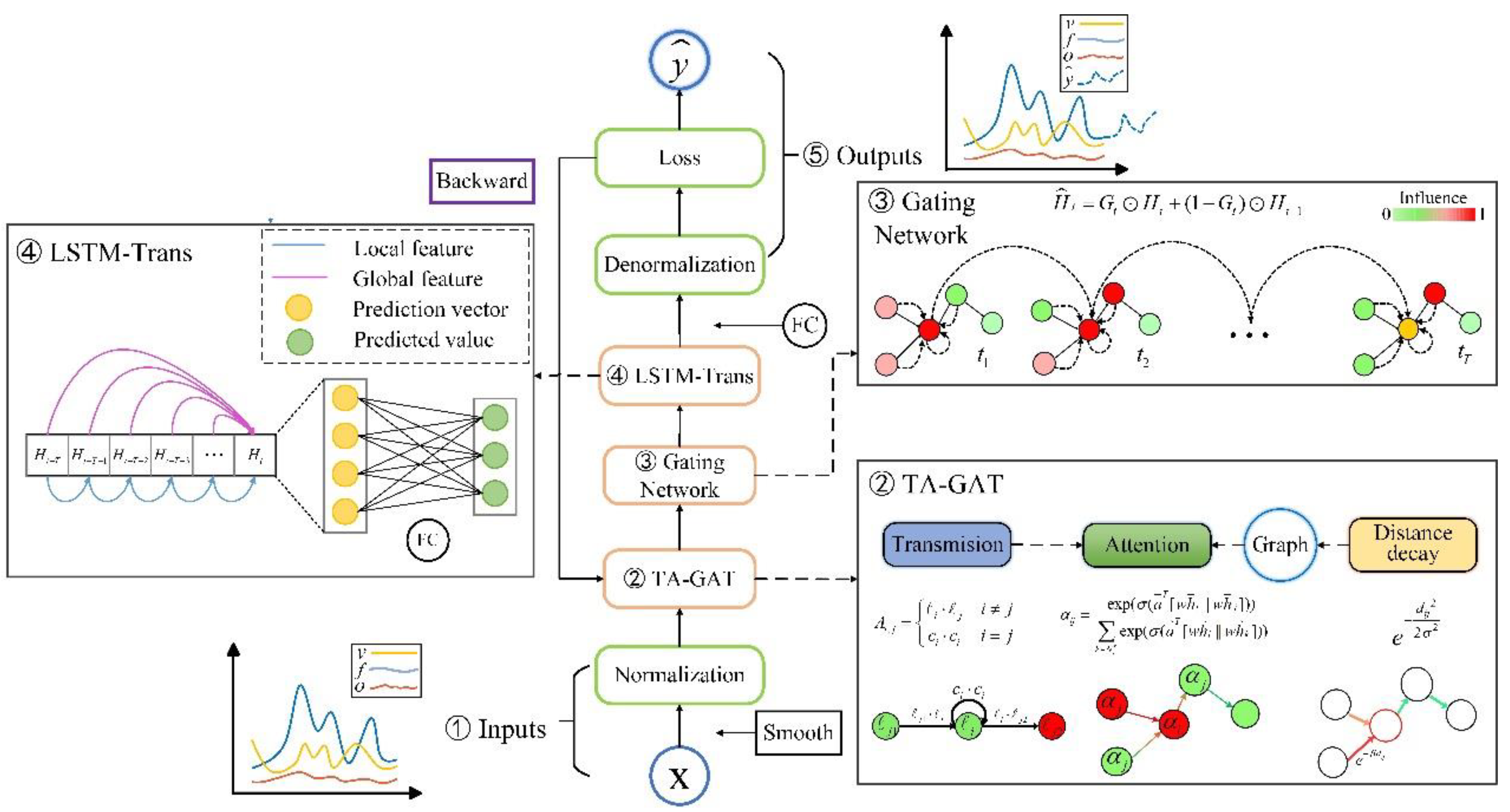
Figure 3.
GAT model with a multi-head attention mechanism.
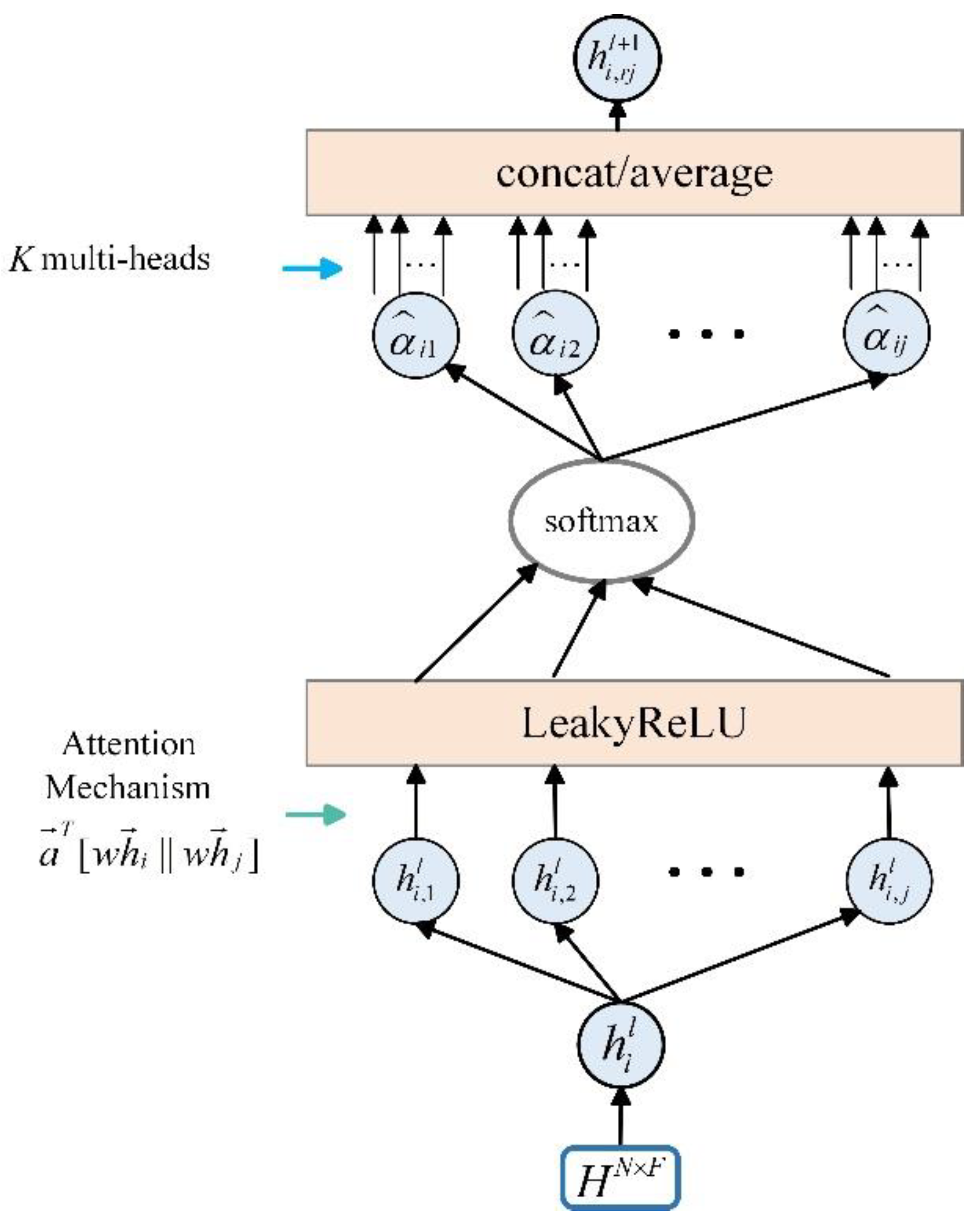
Figure 4.
Node transfer probability diagram.
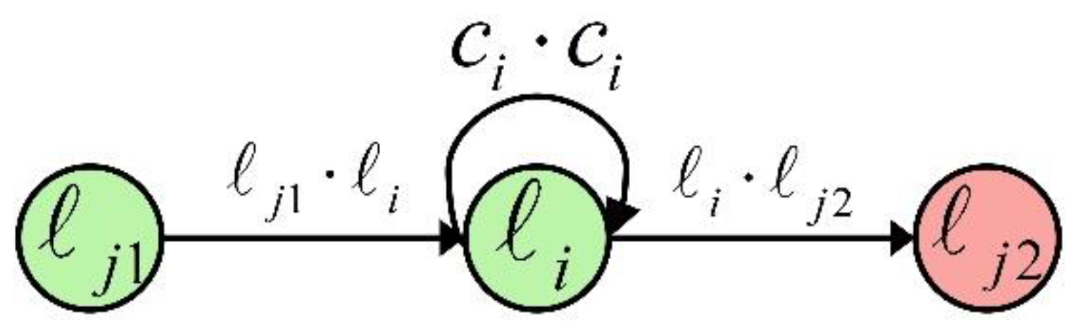
Figure 5.
The TA-GAT module.
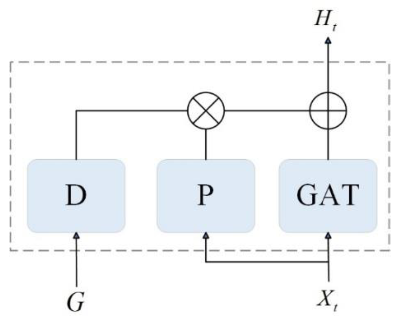
Figure 6.
Gating Network diagram.
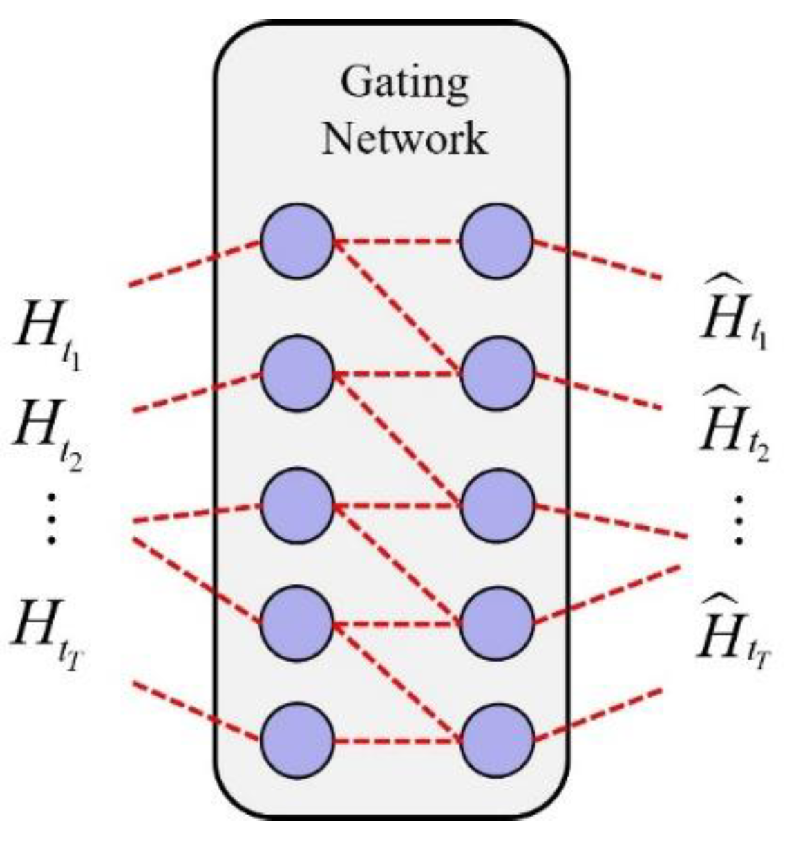
Figure 7.
The LSTM-Trans module. (a) LSTM (b) Transformer Encoder.
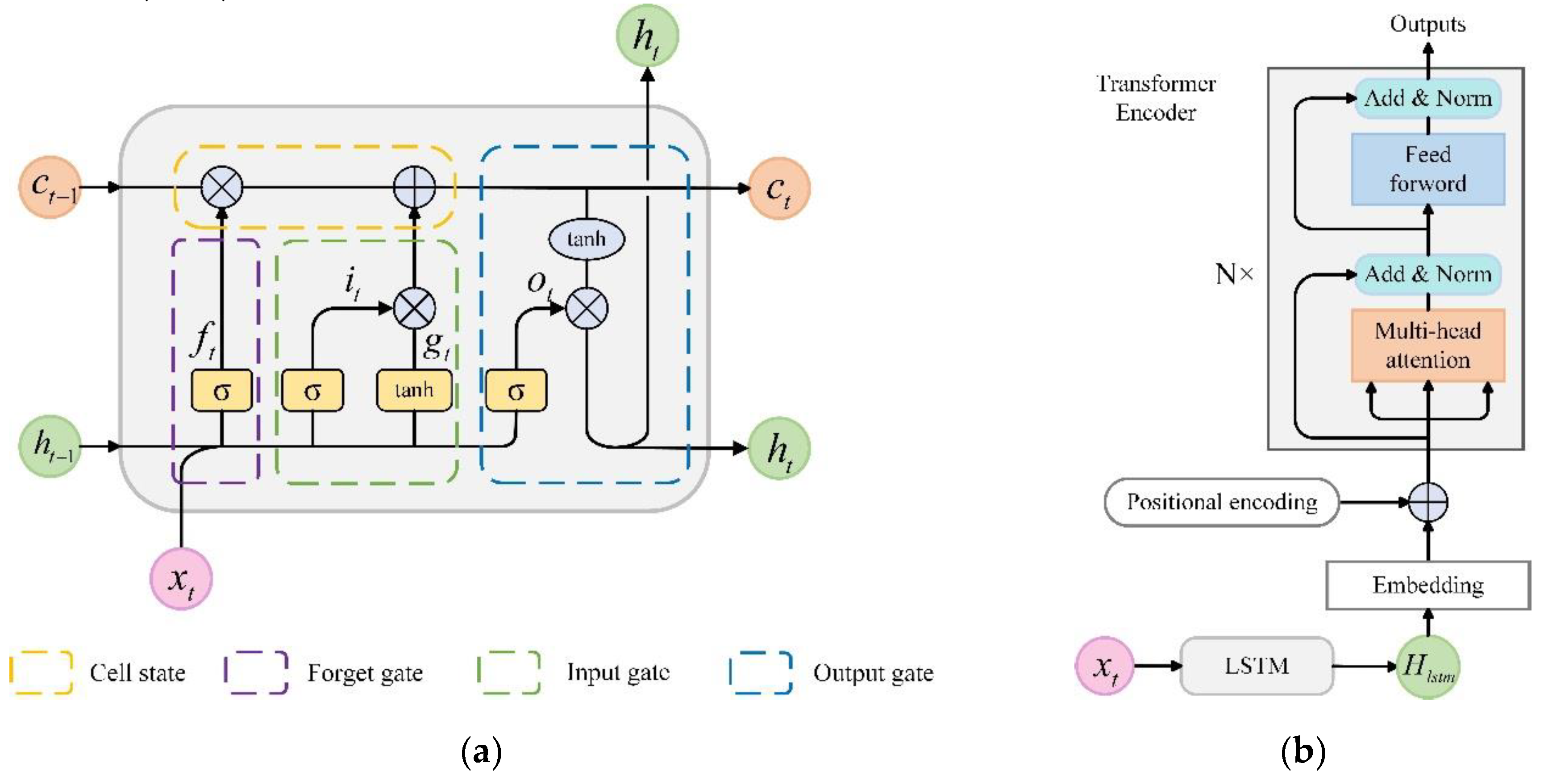
Figure 8.
Comparison of prediction results on PeMS03 and PeMS04. (a) The results of testing on PeMS03; (b) The results of testing on PeMS04.
Figure 8.
Comparison of prediction results on PeMS03 and PeMS04. (a) The results of testing on PeMS03; (b) The results of testing on PeMS04.
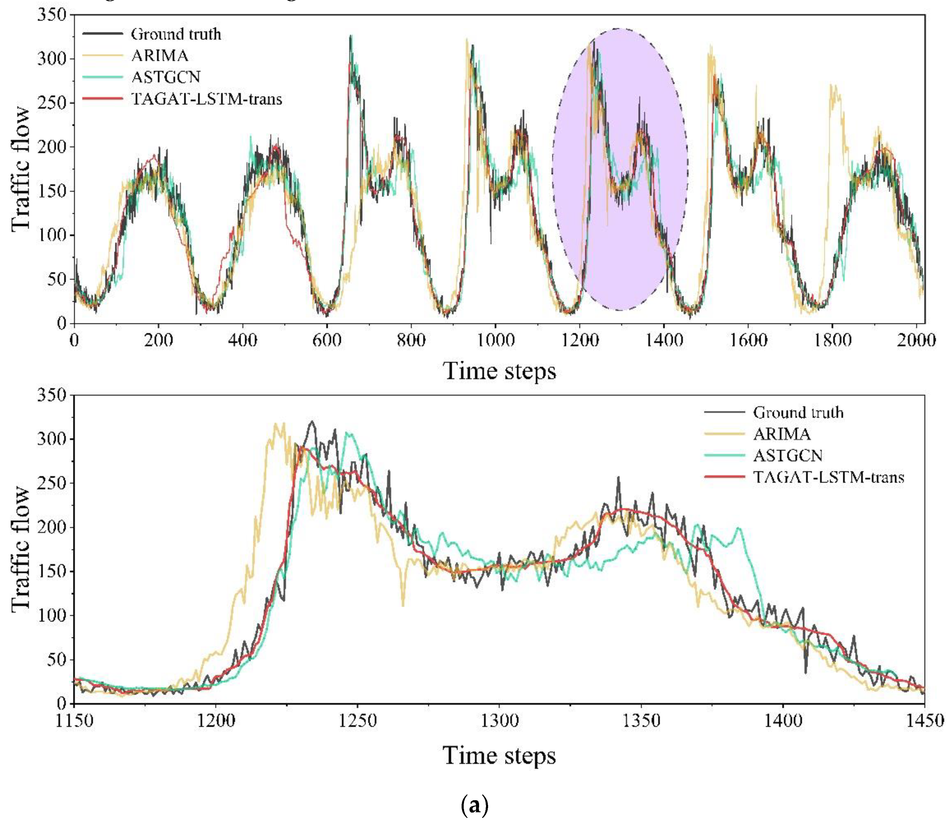
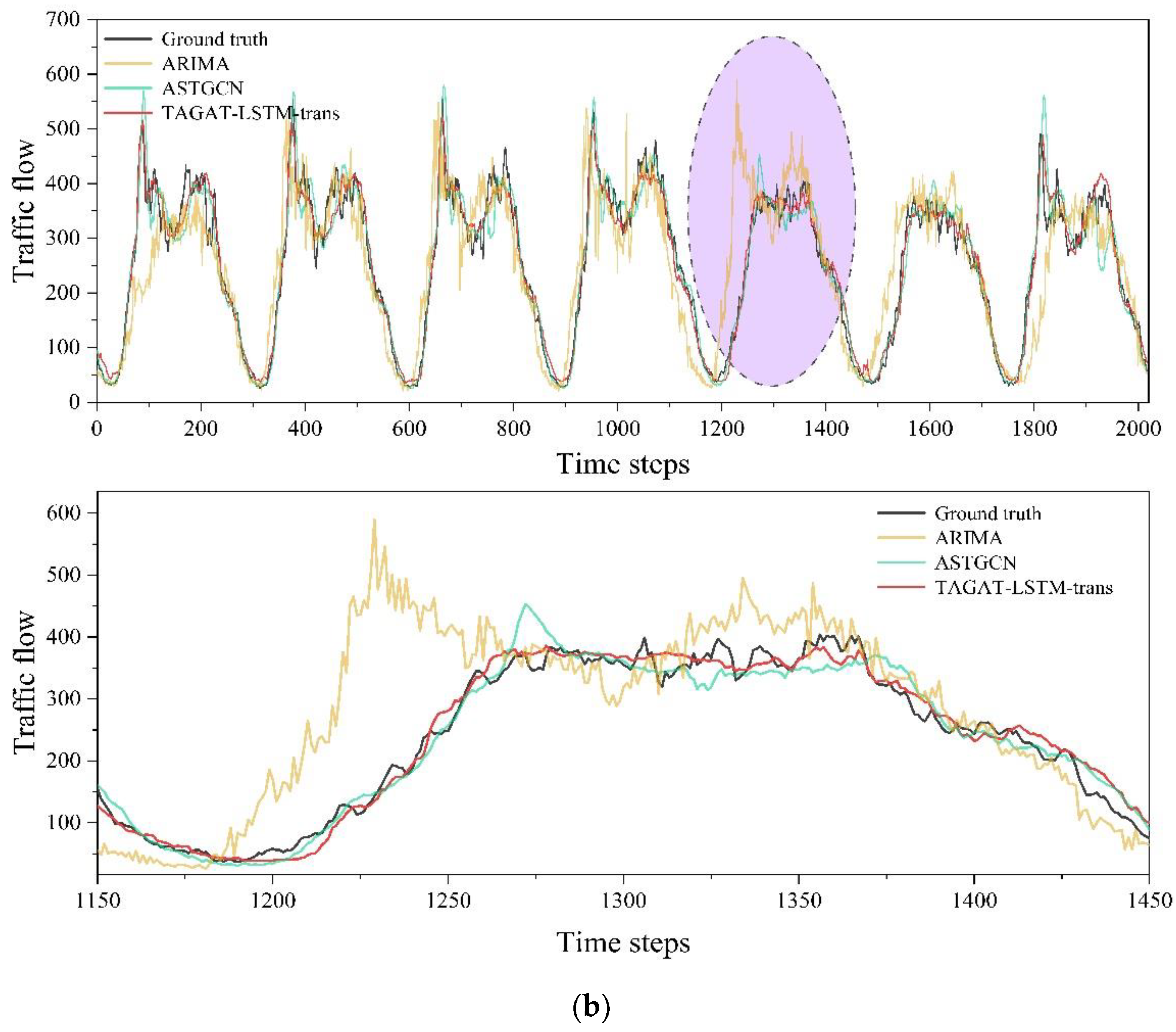
Figure 9.
Comparison of scatter plot on PeMS03 and PeMS04. (a) The scatter plot on PeMS03; (b) The scatter plot on PeMS04.
Figure 9.
Comparison of scatter plot on PeMS03 and PeMS04. (a) The scatter plot on PeMS03; (b) The scatter plot on PeMS04.
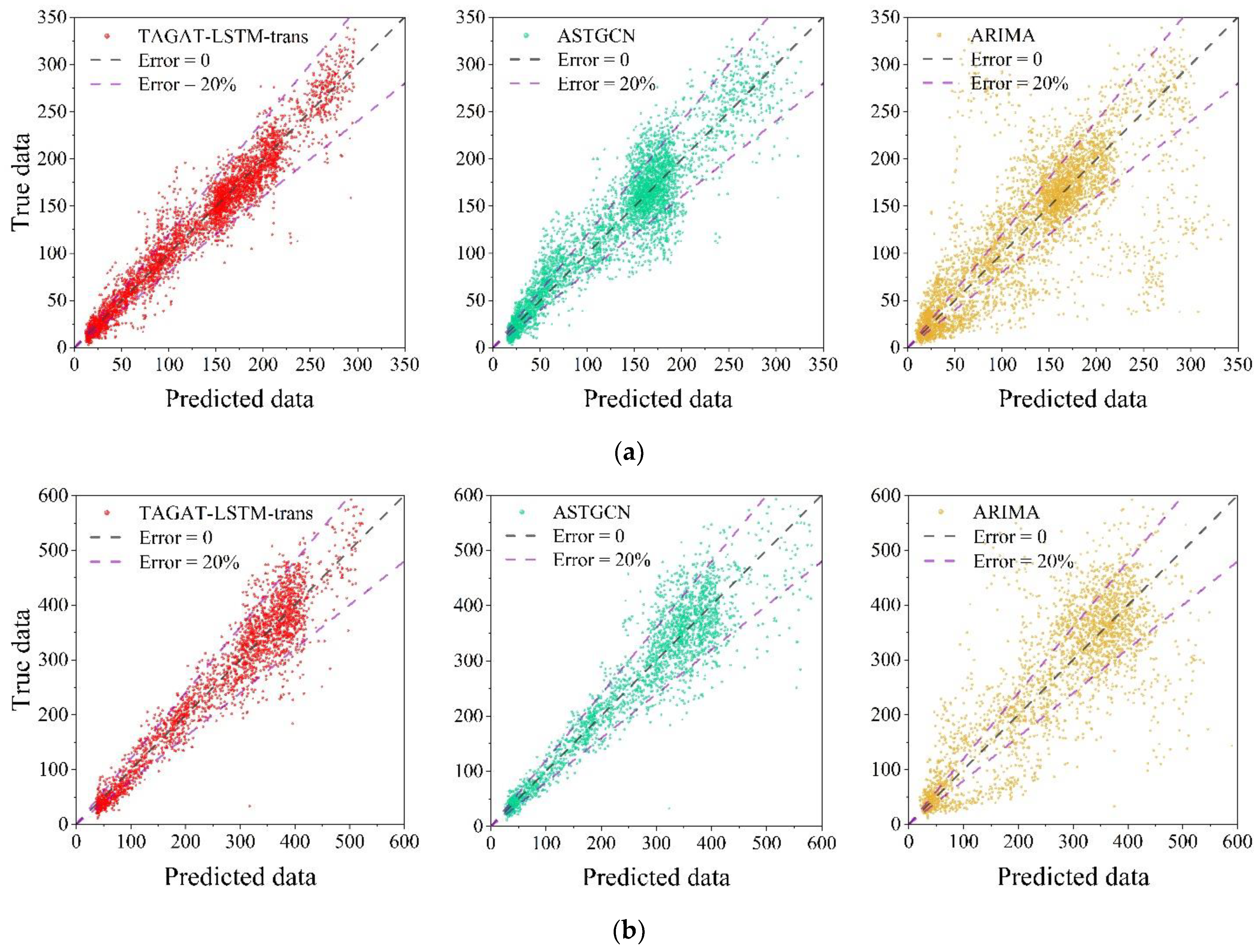
Figure 10.
The results of ablation experiments on PeMS03 and PeMS04. (a) PeMS03; (b) PeMS04.
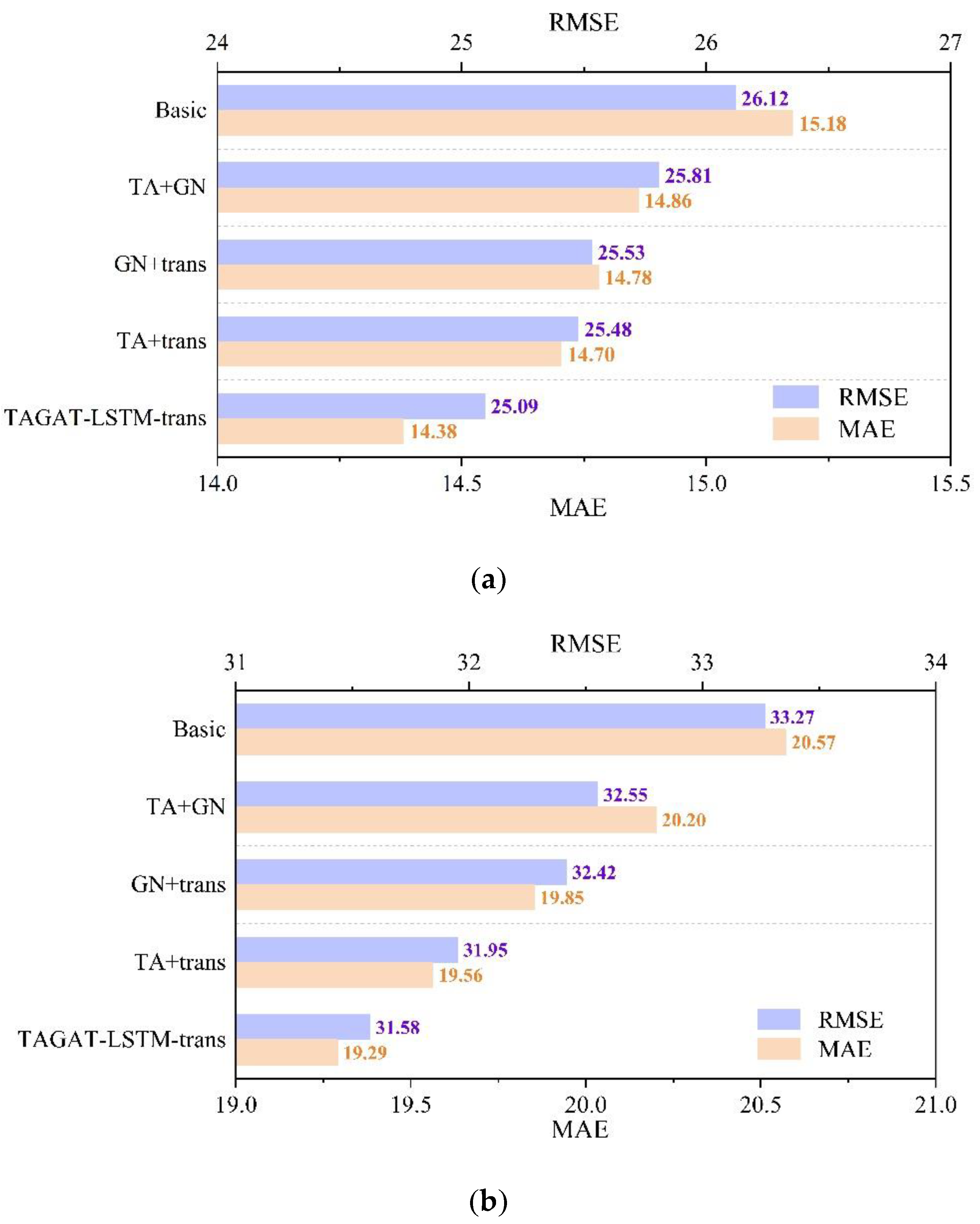

Table 1.
Dataset description.
| Datasets | Sensors | Edges | Time |
|---|---|---|---|
| PeMS03 | 358 | 547 | 09/01/2018 - 11/30/2018 |
| PeMS04 | 307 | 340 | 01/01/2018 - 02/28/2018 |
Table 2.
Model hyperparameters.
| Module | Hyperparameters | Numbers |
|---|---|---|
| TAGAT | Hidden units | 32 |
| Attention heads | 2 | |
| LSTM | Hidden units | 256 |
| Layers | 2 | |
| Transformer | Hidden units | 256 |
| Attention heads | 4 | |
| Other | Batch size | 50 |
| Learning rate | 5e-4 | |
| Dropout | 0.1 |
Table 3.
Comparison of the mean performance of various methods on PeMS03 and PeMS04.
| Model | PeMS03 | PeMS04 | ||
| МАЕ | RMSE | MAE | RMSE | |
| ARIMA | 23.07 | 40.62 | 37.84 | 59.03 |
| VAR | 23.65 | 38.26 | 33.76 | 51.73 |
| LSTM | 21.33 | 35.11 | 27.14 | 41.59 |
| DCRNN | 18.18 | 30.31 | 24.70 | 38.12 |
| ASTGCN(r) | 17.69 | 29.66 | 22.93 | 35.22 |
| STDSGNN | 16.12 | 25.59 | 20.67 | 32.40 |
| TAGAT-LSTM-trans | 14.38 | 25.09 | 19.29 | 31.58 |
Disclaimer/Publisher’s Note: The statements, opinions and data contained in all publications are solely those of the individual author(s) and contributor(s) and not of MDPI and/or the editor(s). MDPI and/or the editor(s) disclaim responsibility for any injury to people or property resulting from any ideas, methods, instructions or products referred to in the content. |
© 2025 by the authors. Licensee MDPI, Basel, Switzerland. This article is an open access article distributed under the terms and conditions of the Creative Commons Attribution (CC BY) license (http://creativecommons.org/licenses/by/4.0/).
Copyright: This open access article is published under a Creative Commons CC BY 4.0 license, which permit the free download, distribution, and reuse, provided that the author and preprint are cited in any reuse.


