Submitted:
02 October 2025
Posted:
04 October 2025
You are already at the latest version
Abstract
Microelectromechanical systems (MEMS) are increasingly used for both industrial and consumer applications. To improve the accuracy and efficiency of MEMS fabrication and to overcome the limitations of conventional contactless positioning systems, this study introduces a novel positioning concept that combines ultrasonic levitation with electromagnetic actuation. Squeeze-film effects generated by high-frequency ultrasonic transducers enable levitation, while fast-response reluctance forces from electromagnets govern the positioning dynamics without requiring bulky mounting frames. A novel double-acting ultrasonic transducer with a Gaussian-profile horn is proposed, ensuring approximately uniform vibration distribution and increased levitation force. The double-acting design enables levitation on both surfaces, simplifying mounting and reducing interactions among transducers. A model-based control strategy ensures resonant operation and constant vibration amplitude. Experiments demonstrate levitation forces up to 343 N, with a total levitation height of 25 μm, resulting from two levitation air gaps. Comprehensive performance characterization validates the feasibility of this transducer design for integration into the proposed positioning system.
Keywords:
squeeze-film ultrasonic levitation
; double-acting piezoelectric transducer
; horn geometry optimization
; model-based resonance control
1. Introduction
Microelectromechanical systems (MEMS) are essential components in a wide range of modern technologies and have experienced remarkable market growth in recent decades. From early physical sensors such as accelerometers and gyroscopes to more recent flexible sensors for wearable devices, MEMS have found applications in both industrial and consumer domains. Their fabrication processes, however, demand extremely high precision in positioning and alignment, as exemplified by pad alignment in wire bonding, encapsulation, and wafer-level packaging [1,2].
To improve the accuracy and efficiency of the MEMS fabrication, recent research has increasingly focused on functional integration and the development of novel positioning system configurations. In this context, we present an approach which combines ultrasonic levitation with electromagnetic actuators to meet the growing performance requirements of MEMS manufacturing. Compared with conventional contactless positioning system such as hydrostatic and purely electromagnetic solutions, the proposed technology offers several advantages. First, it requires no external media such as compressed air or oil. Second, it overcomes the need for bulky frames to mount counteracting pairs of electromagnets [3]. Instead, the levitation force is generated by the squeeze film effect induced by the high frequency vibration (≈ 20 kHz) of ultrasonic transducers, while the positioning dynamics are controlled by electromagnets whose reluctance forces provide a fast response [4]. This paper presents the design and control strategy of a novel double-acting piezoelectric ultrasonic transducer that ensures a significant increase in load capacity while maintaining stable levitation. A geometry optimization resulted in the development of a particular horn with Gaussian side profile. This specific geometry ensures a balance between achieving a uniform vibration distribution across the horn surface and enlarging the transducer output surface to enhance the levitation force. The term double-acting refers to the capability of the transducer to generate levitation air gap on both of its output surfaces. This configuration not only simplifies the mounting concept but also minimizes undesired interactions among multiple transducers. To guarantee resonant operation with a constant vibration amplitude, a model-based control strategy has been utilized.
2. Novel Transducer Design
2.1. Squeeze-Film Levitation
Acoustic levitation can be broadly classified into standing-wave levitation and squeeze-film levitation (also referred to as near-field levitation) [5]. Figure 1 illustrates representative configurations of both principles, each of which allows the suspension of objects with relatively large dimensions. In the case of standing-wave levitation, shown in Figure 1(a), the levitated object itself acts as the reflector, thereby forming a standing-wave field between the transducer and the object. The levitation force arises from the acoustic radiation pressure exerted on the planar surface of the object within this field. In principle, the dimensions of the levitated objects are not constrained by the acoustic wavelength. However, this method provides only a limited load capacity and is thus typically restricted to lightweight objects, such as thin planar disks [6]. When the distance between the transducer and the reflector is reduced to the micrometer scale, squeeze film levitation occurs Figure 1(b). In this case, high-frequency vibration generates a thin air film between the transducer and the reflector, producing an overpressure that suspends the reflector (see Figure 1(c)). Compared with standing-wave levitation, this effect enables the support of significantly heavier objects. For this reason, this paper focuses primarily on squeeze-film levitation.
Given the use of squeeze-film levitation, the governing equation for calculating the levitation force is derived from Reynolds’ equation rather than from acoustic radiation pressure [7]. The equation is expressed in polar coordinates.
It is to be note that h in the equation denotes transient absolute levitation height and must be calculated according to Equation (2).
Here, denotes the averaged steady state levitation distance, is the vibration amplitude of the transducer, and is the angular excitation frequency. For numerical calculation, the equation is normalized. Furthermore, is the ambient air pressure and is the radius of the transducer’s output surface.
Since it is straightforward to excite angular plate vibration modes with antinodes located at the center, only these types of modes are considered. In this case, the vibration amplitude along the angular direction remains constant. The normalized equations are presented below. In Equation (5) the angular coordinate is no longer a variable.
Two key parameters are introduced. The first is the compression ratio in Equation (4), which governs the magnitude of overpressure. The second is the squeeze-number in Equation (5), which characterizes the time required for the generated overpressure to reach steady state. Lager values of correspond to longer response times. The vibration mode of a thin angular plate is represented by Equation (6) [8]. The subscript zero indicates the absence of nodal diameters. The functions and denote the zero-order Bessel function and the modified Bessel function of the first kind, respectively. The constants and are determined by the boundary conditions and the mode number.
To solve Reynolds’ equation for different vibration modes, the displacement function is substituted into Equation (1). Figure 2(a) illustrates the normalized steady-state overpressure distribution along the radius of the transducer output surface. For a uniform displacement distribution, i.e., without node circles, the highest value and uniform distribution of overpressure are obtained. In contrast, the presence of node circles significantly reduces the overpressure in those regions, thereby lowering the overall overpressure. As shown in Figure 2(c), the average overpressure decreases sharply with an increasing number of node circles. For instance, with two node circles, it drops to only 17% of the value achieved without node circles. To achieve a higher levitation force, transducers with larger output surfaces appear advantageous. However, enlarging the surface area leads to uneven vibration amplitudes, as flexural modes emerge beyond a certain radius. To overcome this issue, a geometry optimization was performed.
2.2. Geometry Optimization
At first, the objectives and constraints of the optimization must be clearly defined. The primary objective is to maximize the levitation force, which requires a larger transducer output surface. However, as noted earlier, the vibration amplitude distribution need to remain uniform, and the number of vibration node circles must be carefully considered. The main constraints are that the transducer must operate at a natural frequency within the ultrasonic range and adopt a configuration to ensure compactness. Figure 3(a) illustrates models, which feature two distinct radii, 40 mm and 70 mm, and five distinct side profiles: Gaussian, quadratic, cubic, exponential, and linear. The two radii correspond to cases without node circles and with a single node circle, respectively. Due to compactness requirements of integration in positioning system, radii larger than 70 mm are not considered. Different side profiles are investigated to achieve a uniform vibration amplitude. In this way the mass near the horn input surface or at the rim of the horn output surface can be differently distributed. As a result, the deformation uniformity of the output surface can be influenced accordingly. For example, in the model with the exponential profile the rim is at thinnest, which leads to the lowest mass and therefore the largest deformation at the rim. In contrast, for the cubic side profile, the mass near both the input surface and the output rim is higher than in other cases. Consequently, the deformation distribution of the output surface is more uniform. Thus, the choice of side profile determines the balance between rim and center deformation and need to be consider for small and large radii. These two models are used for modal analysis in ANSYS and represents the horn and half of the piezo-rings. The input surface is fixed in the longitudinal direction because it is where the vibration node for the transducer is located. Its radius is set equal to that of commercially available piezo-rings (50 mm diameter). The deformation of the output surface is subsequently normalized with respect to the reaction force at the fixed input surface. This reaction force represents the excitation required to generate the observed deformation and provides a consistent basis for comparing the deformation under identical excitation levels.
The normalized deformations are presented in Figure 3(c) and (d), while Figure 3(b) illustrates the corresponding average and standard deviation. The average deformation represents the vibration level under identical excitation, whereas the standard deviation quantifies the uniformity of the amplitude distribution. With the exception of the exponential side profile, models with larger radii exhibit lower mean amplitudes than those with smaller radii due to the presence of node circles. The side profiles, however, exert only a minor influence on the uniformity of the amplitude distribution. The exponential profile produces large edge deformation; consequently, the mean and standard deviation are the largest. Since the objective is to maximize the levitation force, it is necessary to calculate the levitation force using Equation (5) to select an optimal side profile. Figure 4(a) and (b) present the numerical solutions for two different radii and five side profiles. As expected, models with a radius of 40 mm exhibit large average deformation and consequently higher overpressure. For a radius of 70 mm, the numerically calculated overpressure follows the deformation distribution: it is higher in the middle and on the edge, but significantly reduced in the region of the node circle. The levitation forces are obtained by multiplying the calculated overpressure with the discretized surface area. The results are presented in Figure 4(c). As expected, larger surface areas result in greater levitation forces, even in the presence of node circles. Among the five discussed side profiles, the linear and Gaussian profiles provide the highest levitation forces. The Gaussian profile was ultimately selected because its reduced deformation amplitude near the edge prevents overloading at the transducer rim and mitigates wear between the transducer edge and the ground reflector. Additionally, the simulation results indicate that the profile under consideration exhibits a reduced strain near the rim, thereby decreasing the probability of fatigue failure.
2.3. Transducer Assembly and Characterization
In the positioning system, three transducers are integrated to achieve a stable position control (one out-of-plane displacement and two Tait-Bryan-angles), while also to provide larger load capacity. In practice, however, manufacturing tolerances make it economically impractical for all transducers to share the same resonance frequency. When multiple transducers are employed, low-frequency vibration modes of the housing structure can be excited by the frequency mistuning, which can damage the positioning stability. This issue is effectively mitigated by adopting the double-acting concept. The final structure consists of two identical horns with a Gaussian side profile. The final output surface diameter is selected as 120 mm to maintain the resonance frequency above 20 kHz, while the horn input diameter matches that of the piezo-rings (50 mm). The fixture flange is design for a flexible mounting of transducer within the housing structure. It is implemented with four extremely tear-resistant and very low-stretch ropes coated with Dyneema SK78. These four ropes are pre-tensioned and arranged perpendicularly to each other, thereby constraining only planar movements of the transducer. This flexible fixture has a notable advantage by preventing the transmission of radial vibrations and unavoidable longitudinal vibrations from the fixture flange to the housing structure. On both sides of the fixture flange, one pair of piezoelectric rings is located. Furthermore, a specially washer is used to pre-tension the transducer. This washer prevents the transmission of torsional force from pretensioning directly onto the piezo-rings. Figure 5 illustrates the final assembly of the proposed transducer along with its fixture.
Following the assembly, the transducer was characterized experimentally. Figure 6(a) shows the measured electrical frequency response of the transducer. The resonance frequency is 22.61 kHz. The frequency difference between resonance and antiresonance is 971 Hz. The upper part of Figure 6(b) shows the measured radial distribution of vibration amplitude on both top and bottom output surfaces at a current amplitude of 2 A. The measurement was obtained using an MSA-100-3D-H/V Micro System Analyzer (Polytec). The consistency of the two distributions confirms identical vibration characteristics, thereby ensuring the generation of identical levitation force on both surfaces. The lower part of Figure 6(b) illustrates the electromechanical convertibility of the transducer at resonance, representing the current required to achieve a given area-weighted averaged vibration velocity. A proportional relationship is observed, with a slope of 171.81 mm/As. Due to the presence of a node circle, this value of 171.81 mm/As is notably lower than the vibration amplitude observed at the center or edge of the output surface.
3. Transducer Control Strategy
The manufactured transducer exhibits a weakly damped property (), as evidenced by the significant amplitude increase and the distinct phase zero crossing at resonance. In addition, a linear electromechanical convertibility was characterized at resonance. In this case, the transducer should be operated at its resonance. The operating point offers several advantages. From a mechanical perspective, the vibration amplitude reaches its maximum at resonance. From an electrical perspective, the absence of reactive power is ensured, since voltage and current are in phase. Moreover, the transient vibration response at resonance exhibits a PT1 characteristic, i.e., without beating or oscillation in the transient response [9]. As shown in Figure 6(b), the velocity is proportional to the current amplitude at resonance. Thereby, when the current is controlled to a constant value, both the vibration velocity and the resulting levitation force remain constant. On this basis, the control strategy is designed to ensure resonant operation of the transducer.
The modal reduction method is a well-established approach for calculating the system response to dynamic excitation. In ultrasonic transducers, operations are typically concentrated in the vicinity of a single isolated resonance, most commonly the longitudinal vibration mode. This mode can be accurately represented by a model with one and a half degrees of freedom (DoF), whose corresponding equivalent electrical circuit is shown in Figure 7. Here, the DoF refers to the electrical charge rather than mechanical deformation. The parameters of the equivalent circuit were identified from the measured electrical frequency response and are summarized in Table 1.
In ultrasonic systems, control typically focuses not on the high-frequency vibrations themselves but rather the amplitudes and phase between current and voltage. Since the system dynamics are much slower than the ultrasonic frequency, this simplified consideration proves both practical and effective. In practice, phase shifts between current and voltage can only be realized by varying the excitation frequency, whereas the current amplitude is controlled by adjusting the voltage amplitude. Therefore, in the proposed model the excitation frequency and voltage amplitude are defined as inputs, while the current amplitude and the phase shift between voltage and current defined as outputs. This constitutes the key innovation of the model [10]. Starting with the differential equation of the equivalent circuit, which is shown below:
The slowly time-varying complex amplitude of current—consisting of both magnitude and phase—is substituted into Equation (7). Taylor expansion is then applied to linearize the expression, with higher-order terms neglected. After further mathematical manipulations (for a detailed derivation, see [10]), the model is obtained in state-space representation:
From this state-space representation, four transfer functions can be derived. Among these, two are particularly important: the frequency vs. phase and the current vs. voltage amplitude. Under the assumption of weak damping and resonant operation, these functions can be simplified as follows:
Both transfer functions exhibit PT1 behavior, making a PI-controller suitable for implementation. The control parameters are subsequently determined using the pole-placement method [10,11]. The proposed PI controllers were implemented in a Rapid Control Prototyping system (MicroLabBox from dSPACE). Figure 8 illustrates the control architecture, which consists of two main parts: phase and amplitude detection, implemented on the FPGA, and two PI controllers, implemented on the microcontroller. Phase and amplitude detection is realized using phase-sensitive demodulation [12]. Its advantage lies in its robustness against noise and higher-order harmonics, ensuring high accuracy even at low sampling rates and resolution. The two parallel PI controllers perform phase-zero and current amplitude control, respectively. The control algorithm uses a maximum control frequency of 10 kHz.
4. Results and Discussion
The levitation performance of the manufactured transducer in Figure 5 was characterized using the program in Figure 8. The experiment setup is shown in Figure 9(a), and the measured load characteristic map is presented in Figure 9(b). Following key parameters are considered: levitation force, total levitation height from two air gaps, and averaged vibration amplitude. Unlike previously reported experiments [6,13], where the reflector was gradually pushed toward a transducer already operating in steady state, the experiments in this study were conducted with the weights already placed on the transducer. Stable levitation was then achieved simply by switching on the transducer. In this case, the settling of the transducer vibrations and the generation of the levitation air gap occur simultaneously. By linearly increasing the current amplitude from 1 A to 3 A using a ramp function, the vibration amplitude of the transducer increased linearly from 1.21 m to 3.63 m. The levitation force corresponded to the customized weights suspended during the experiment, while the levitation height was measured using an eddy-current sensor. Due to the double-acting principle of the transducer, the measured levitation height corresponds to the sum of the air gaps on both output surfaces.
The projection of the load map onto the levitation force–height plane (red dashed line) reveals a nonlinear relationship at constant vibration amplitude, indicating that the air-gap stiffness increases nonlinearly as the levitation height decreases. In contrast, the projection onto the vibration amplitude–height plane (black dashed line) shows a clear linear relationship between vibration amplitude and levitation height at constant load. This confirms the feasibility of integrating the transducer into the position control loop using a linear control approach. With increasing load, this linear trend persists, although the slope decreases. This implies that larger vibration amplitudes are required to achieve the same increment in levitation height when the transducer or the positioning system operates under high load. Overall, the experiments demonstrate that a single transducer is capable of generating a levitation force of 294 N and a total levitation height of 29 m from off-state. In this case, the averaged vibration amplitude reached 5.7 m. When the weights were placed after the transducer had already reached steady state, an even higher load capacity of 343 N at the same averaged vibration amplitude was measured. The corresponding levitation height was reduced to 25 m. Both the levitation force and levitation height exceed previously reported values at standard ambient pressure, such as those in [6,13] (> 100 N and 146.7 N force, respectively).
The final configuration of the micro-positioning system is illustrated in Figure 10. It consists of three ultrasonic transducers and three electromagnetic actuators. Accordingly, the control algorithm of the ultrasonic transducers is replicated threefold, with each running in parallel (see Figure 8). The electromagnetic actuators are utilized to adjust the position of the system due to their faster response. Experimental results on the levitation performance of the positioning system are reported [14].
5. Conclusions
This paper has presented the design and control of a novel double-acting ultrasonic transducer for integration into a micro-positioning system. Through geometry optimization, a Gaussian side profile was identified as the most effective horn configuration for providing a high levitation force. The double-acting concept allows levitation on both transducer surfaces, thereby simplifying mounting concept and reducing undesired interactions among multiple transducers. A model-based control strategy was implemented to guarantee resonant operation with constant vibration amplitude. The measured characteristic load diagram showed that the stiffness of the air gap increasing rapidly as levitation height decreases at constant vibration amplitude. In this case, position control of the system is strongly dependent on the operating point. Thus, the design of an adaptive control loop should be considered. Additionally, a linear relationship between current (i.e. vibration amplitude) and levitation height under constant load conditions was confirmed. This demonstrates the feasibility of integrating the transducer into the system’s position control loop, thereby reducing system overall power consumption and heat generation. In terms of load capacity, a single double-acting transducer can lift a load of 294 N simply by being switched on and subsequently sustain stable levitation. The corresponding total levitation height is 29 m, resulting from two air gaps. An even higher load capacity of 343 N at the same averaged vibration amplitude was measured, when the load was increased after the transducer had reached steady state. If necessary, a higher levitation force can be achieved by increasing the vibration amplitude (i.e. current amplitude) and improving surface roughness.
Author Contributions
Conceptualization for ultrasonic transducers, Z.C.; conceptualization for electromagnetic actuators, C.D.; methodology, Z.C.;software, Z.C.;validation for ultrasonic transducers, Z.C.; positioning system’s assembly, C.D.; formal analysis, Z.C; data curation, Z.C; resources, B.D. and J.W.; writing—original draft, Z.C.; supervision, J.T., H.B.; project administration, J.T., H.B.; funding acquisition, B.D. and J. W. All authors have read and agreed to the published version of the manuscript.
Funding
This research was funded by the German Research Foundation (DFG), grant number 456453238.
Conflicts of Interest
The authors declare no conflicts of interest. The founders had no role in the design of the study; in the collection, analyses, or interpretation of data; in the writing of the manuscript; or in the decision to publish the results.
Abbreviations
The following abbreviations are used in this manuscript:
| MEMS | Multidisciplinary Digital Publishing Institute |
| PSD | Phase-sensitive demodulation |
| RCP | Rapid Control Prototyping |
References
- Zhu, J.; Liu, X.; Shi, Q.; He, T.; Sun, Z.; Guo, X.; Liu, W.; Sulaiman, O.B.; Dong, B.; Lee, C. Development Trends and Perspectives of Future Sensors and MEMS/NEMS. Micromachines 2020, 11, 7. [Google Scholar] [CrossRef] [PubMed]
- Huang, Y.; Sai Sarathi Vasan, A.; Doraiswami, R.; Osterman, M.; Pecht, M. MEMS Reliability Review. IEEE Transactions on Device and Materials Reliability 2012, 12, 482–493. [Google Scholar] [CrossRef]
- Denkena, B.; Dahlmann, D.; Krueger, R. Electromagnetic Levitation Guide for Use in Ultra-Precision Milling Centres. Procedia CIRP 2015, 37, 199–204. [Google Scholar] [CrossRef]
- Reiners, J.; Denkena, B.; Wallaschek, J. Kombinierte Ultraschall-Levitations-Magnetführung; Number Band 11/2022 in Berichte aus dem IFW, TEWISS Verlag: Garbsen, 2022. [Google Scholar]
- Andrade, M.A.B.; Pérez, N.; Adamowski, J.C. Review of Progress in Acoustic Levitation. Brazilian Journal of Physics 2018, 48, 190–213. [Google Scholar] [CrossRef]
- Zhao, S.; Wallaschek, J. A Standing Wave Acoustic Levitation System for Large Planar Objects. Archive of Applied Mechanics 2011, 81, 123–139. [Google Scholar] [CrossRef]
- Salbu, E.O.J. Compressible Squeeze Films and Squeeze Bearings. Journal of Basic Engineering 1964, 86, 355–364. [Google Scholar] [CrossRef]
- Blevins, R.D. Formulas for Natural Frequency and Mode Shape; Van Nostrand Reinhold Co.: New York, 1979. [Google Scholar]
- Mojrzisch, S.; Wallaschek, J. Transient Amplitude Behavior Analysis of Nonlinear Power Ultrasonic Transducers with Application to Ultrasonic Squeeze Film Levitation. Journal of Intelligent Material Systems and Structures 2013, 24, 745–752. [Google Scholar] [CrossRef]
- Ille, I.; Wallaschek, J.; Sextro, W. Modellbasierter, resonanter Betrieb schwach gedämpfter Ultraschallsysteme; Number Band 03/2022 in Berichte aus dem IDS, TEWISS Verlag: Garbsen, 2022. [Google Scholar]
- Ille, I.; Twiefel, J. Model-Based Feedback Control of an Ultrasonic Transducer for Ultrasonic Assisted Turning Using a Novel Digital Controller. Physics Procedia 2015. [Google Scholar] [CrossRef]
- Smith, R.W.M.; Freeston, I.L.; Brown, B.H.; Sinton, A.M. Design of a Phase-Sensitive Detector to Maximize Signal-to-Noise Ratio in the Presence of Gaussian Wideband Noise. Measurement Science and Technology 1992, 3, 1054. [Google Scholar] [CrossRef]
- Li, R.; Li, Y.; Sang, H.; Liu, Y.; Chen, S.; Zhao, S. Study on Near-Field Acoustic Levitation Characteristics in a Pressurized Environment. Applied Physics Letters 2022, 120, 034103. [Google Scholar] [CrossRef]
- Denkena, B.; Wallaschek, J.; Buhl, H.; Twiefel, J.; Ding, C.; Chen, Z. Media-Free and Contactless Micro-Positioning System Using Ultrasonic Levitation and Magnetic Actuators. submitted in Actuators 2025. [Google Scholar]
Figure 1.
(a) Standing wave acoustic levitation with levitating reflector. (b) Levitation force versus levitation distance. (c) Squeeze film levitation.
Figure 1.
(a) Standing wave acoustic levitation with levitating reflector. (b) Levitation force versus levitation distance. (c) Squeeze film levitation.
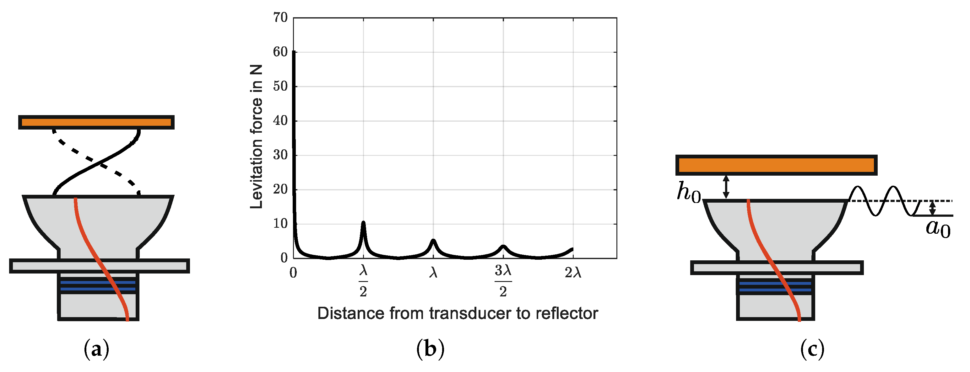
Figure 2.
(a) Numerically calculated normalized steady-state overpressure distribution. (b) Vibration mode of a angular plate with a single node circle. (c) Overpressure generation of the angular plate with increasing node circles.
Figure 2.
(a) Numerically calculated normalized steady-state overpressure distribution. (b) Vibration mode of a angular plate with a single node circle. (c) Overpressure generation of the angular plate with increasing node circles.
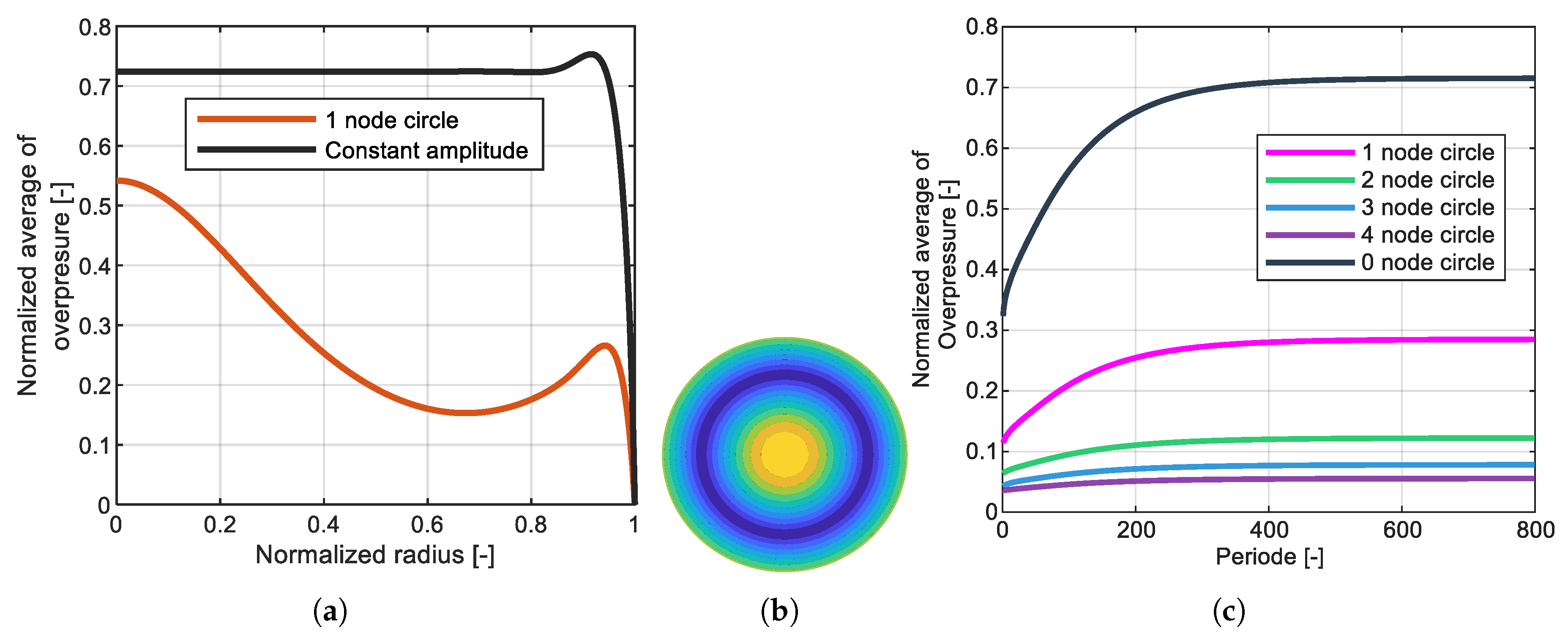
Figure 3.
(a) Different horn side profiles. (b) Average and standard deviation of the normalized deformation. (c) Normalized deformation amplitude of the horn output surface with a radius of 40 mm. (d) Normalized deformation amplitude of the horn output surface with a radius of 70 mm.
Figure 3.
(a) Different horn side profiles. (b) Average and standard deviation of the normalized deformation. (c) Normalized deformation amplitude of the horn output surface with a radius of 40 mm. (d) Normalized deformation amplitude of the horn output surface with a radius of 70 mm.
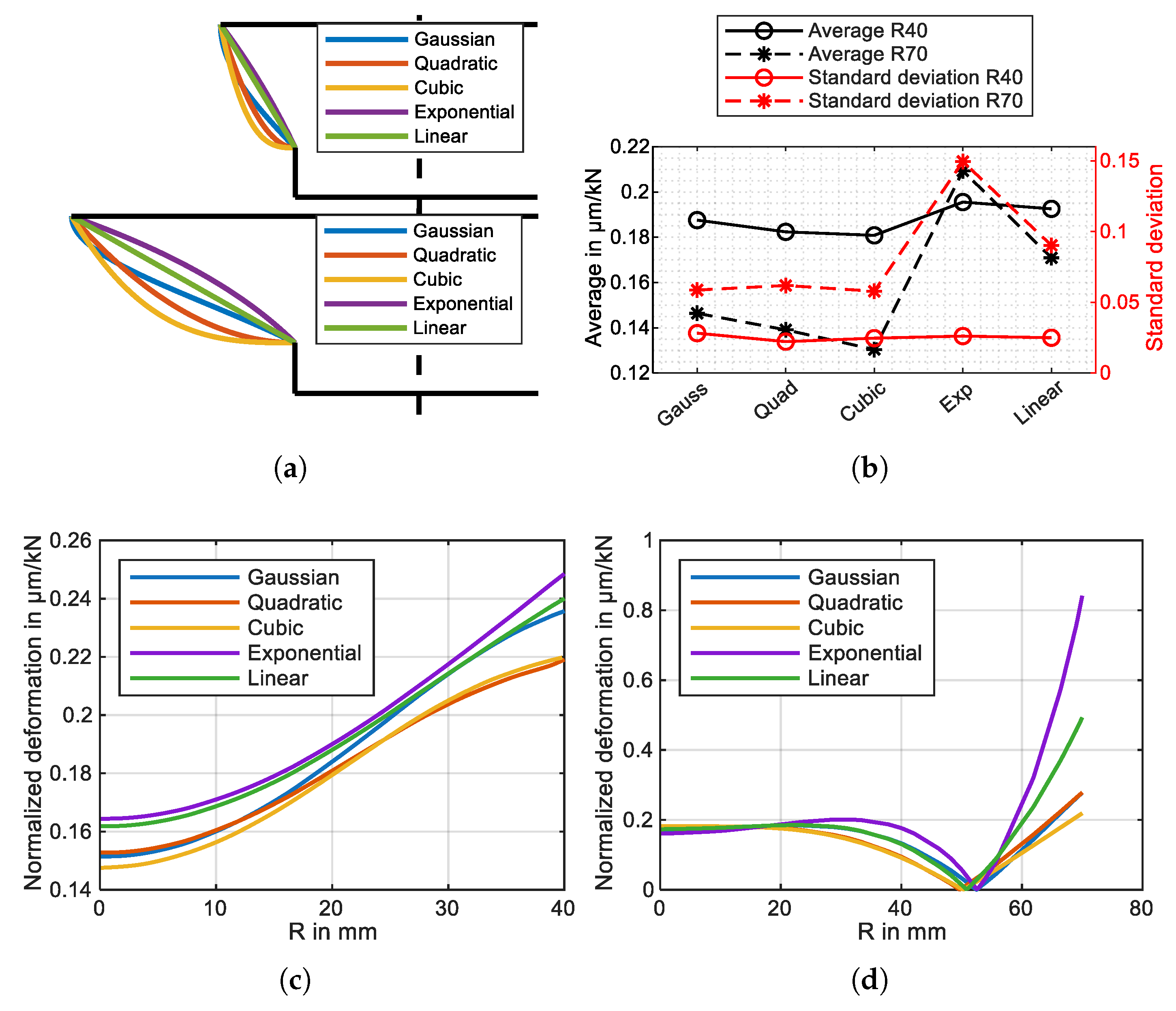
Figure 4.
(a) Numerically calculated normalized overpressure distribution on the horn output surface with a radius of 40 mm. (b) Numerically calculated normalized overpressure distribution on the horn output surface with a radius of 70 mm. (c) Comparison of resulting levitation forces.
Figure 4.
(a) Numerically calculated normalized overpressure distribution on the horn output surface with a radius of 40 mm. (b) Numerically calculated normalized overpressure distribution on the horn output surface with a radius of 70 mm. (c) Comparison of resulting levitation forces.
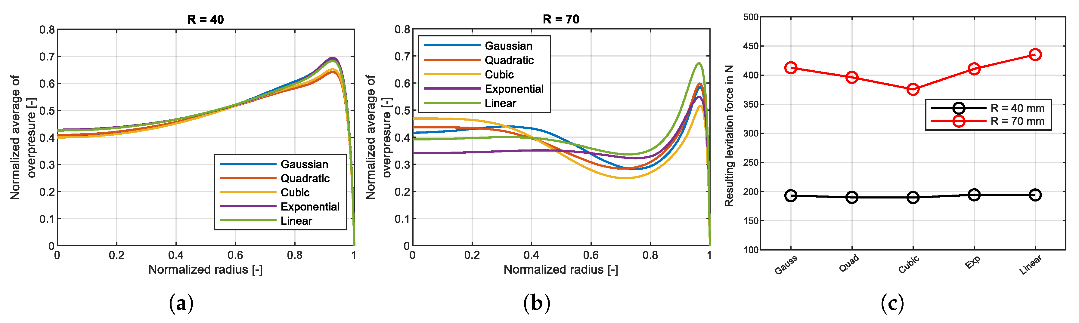
Figure 5.
Manufactured ultrasonic transducer and its fixure methode; schematic sketch of total levitation height.
Figure 5.
Manufactured ultrasonic transducer and its fixure methode; schematic sketch of total levitation height.
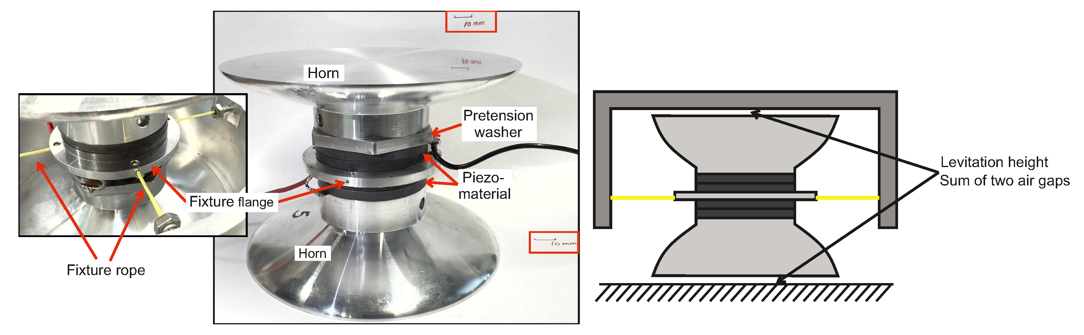
Figure 6.
(a) Measured electric frequency response. (b) Measured radial distribution of vibration amplitude on both output surfaces at a current amplitude of 2 A and the electromechanical convertibility.
Figure 6.
(a) Measured electric frequency response. (b) Measured radial distribution of vibration amplitude on both output surfaces at a current amplitude of 2 A and the electromechanical convertibility.
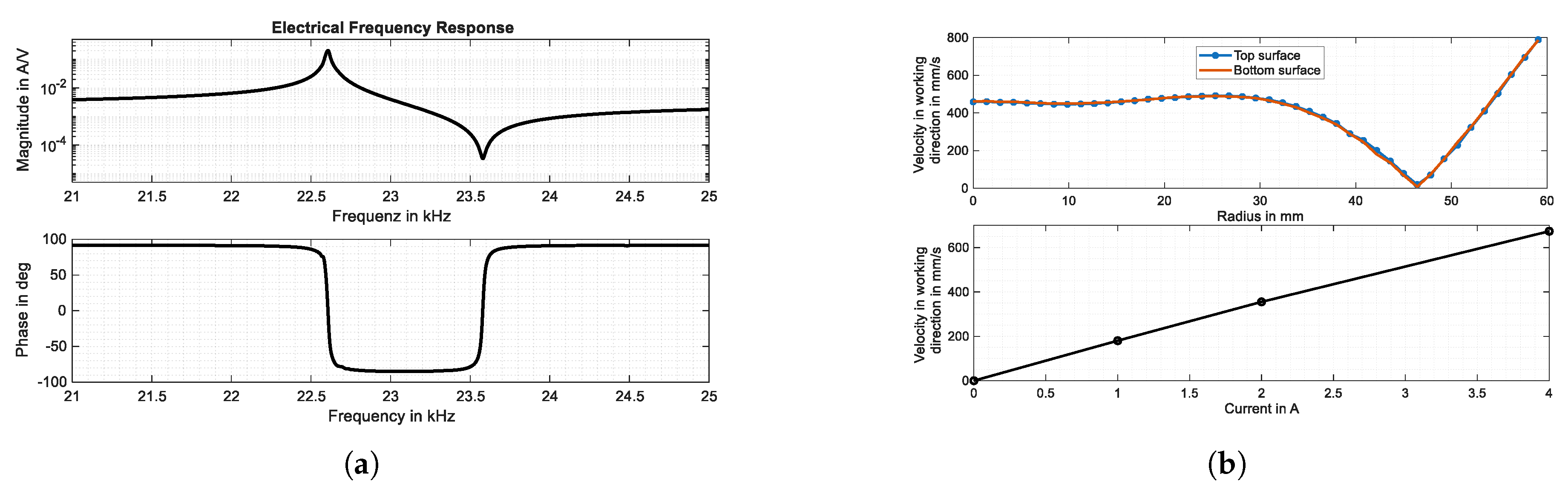
Figure 7.
Equivalent circuit of a piezoelectric transducer.
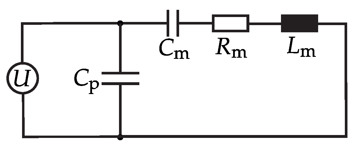
Figure 8.
Control architecture with FPGA and microcontroller.
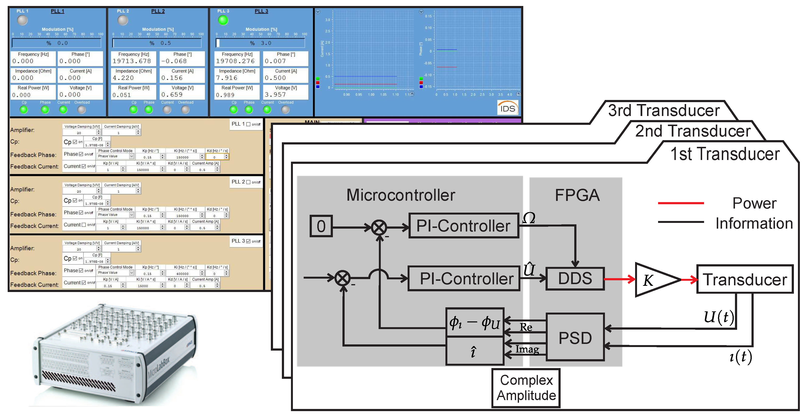
Figure 9.
(a) Experiment setup. (b) Load characteristic map of a single transducer.
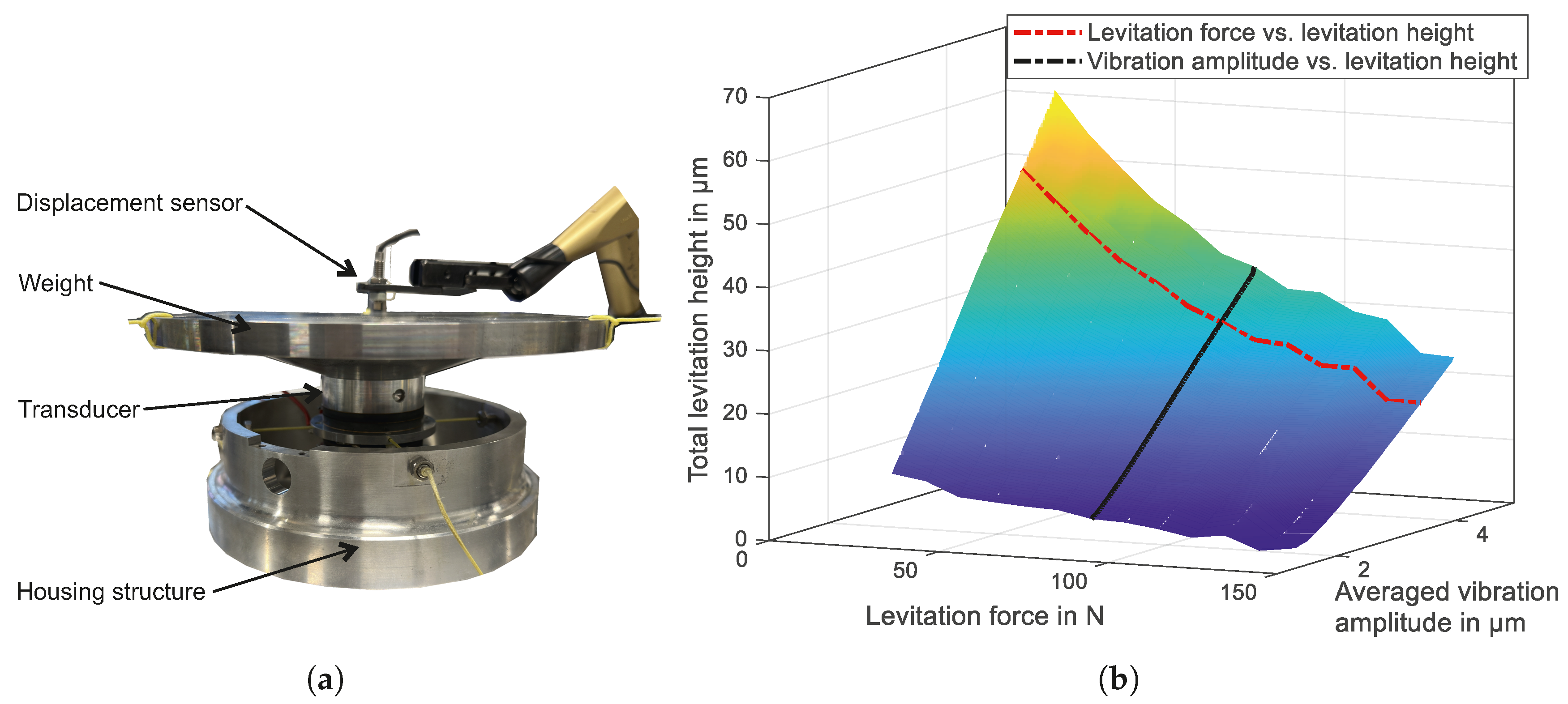
Figure 10.
Design of the final positioning system utilizing ultrasonic transducers and electrical magnet actuators.
Figure 10.
Design of the final positioning system utilizing ultrasonic transducers and electrical magnet actuators.
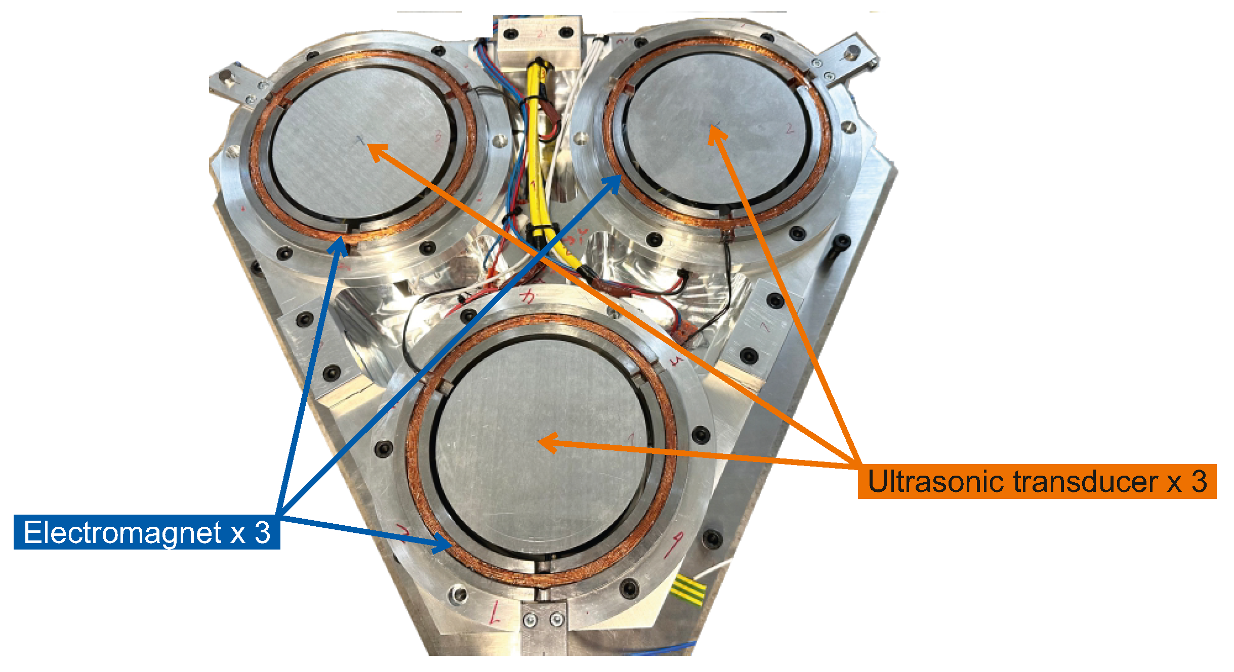

Table 1.
Equivalent circuit parameters for the double-acting transducer.
| Parameter | Value | Unit |
|---|---|---|
| 30.71 | mH | |
| 4.89 | ||
| 1.61 | nF | |
| 18.38 | nF | |
| 890.37 | - | |
| 171.811 | mm/As |
1 Large signal measurement and weighted average across the output surface.
Disclaimer/Publisher’s Note: The statements, opinions and data contained in all publications are solely those of the individual author(s) and contributor(s) and not of MDPI and/or the editor(s). MDPI and/or the editor(s) disclaim responsibility for any injury to people or property resulting from any ideas, methods, instructions or products referred to in the content. |
© 2025 by the authors. Licensee MDPI, Basel, Switzerland. This article is an open access article distributed under the terms and conditions of the Creative Commons Attribution (CC BY) license (http://creativecommons.org/licenses/by/4.0/).
Copyright: This open access article is published under a Creative Commons CC BY 4.0 license, which permit the free download, distribution, and reuse, provided that the author and preprint are cited in any reuse.


