HyperMatrix, SuperHyperMatrix, MultiMatrix, Iterative MultiMatrix, MetaMatrix, and Iterated MetaMatrix

1. Preliminaries

This section gathers the basic notions used throughout the paper. Unless stated otherwise, all sets are taken to be finite.

1.1. Classical Structures, Hyperstructures, and n-Superhyperstructures

A Classical Structure is an ordinary algebraic/relational system on a single carrier. A Hyperstructure is obtained by promoting outcomes of operations to sets (via the powerset). Iterating the powerset n times gives rise to an n-Superhyperstructure; see, e.g., [1,2,3,4,5,6,7,8,9,10]. Intuitively, the n-fold powerset records n layers of “grouping” or aggregation.

Definition 1  

(Base set). Abase setis a nonempty collection S of atomic elements from which we form derived objects such as $\mathcal{P}\left(S\right)$ and the iterated powersets ${\mathcal{P}}^n\left(S\right)$. Formally,

$$S=\{x\mid x\mathit{belongs}\mathit{to}\mathit{the}\mathit{fixed}\mathit{universe}\mathit{under}\mathit{study}\}.$$

Definition 2  

(Powerset). [11] For any set S, thepowerset$\mathcal{P}\left(S\right)$ is the set of all subsets of S:

$$\mathcal{P}\left(S\right)=\{A\subseteq S\}.$$

Definition 3  

(Iterated (nonempty) powersets). (cf. [1,12,13]) Define ${\mathcal{P}}^0\left(H\right):=H$ and inductively

$${\mathcal{P}}^{k+1}\left(H\right):=\mathcal{P}\left({\mathcal{P}}^k\left(H\right)\right)(k\ge 0).$$

Thus ${\mathcal{P}}^1\left(H\right)=\mathcal{P}\left(H\right)$, ${\mathcal{P}}^2\left(H\right)=\mathcal{P}\left(\mathcal{P}\left(H\right)\right)$, and so on. If one wishes to exclude the empty set at each stage, write ${\mathcal{P}}^{*}\left(X\right):=\mathcal{P}\left(X\right)\setminus \{\varnothing \}$ and set ${\mathcal{P}}^{*0}\left(H\right):=H$, ${\mathcal{P}}^{*(k+1)}\left(H\right):={\mathcal{P}}^{*}\left({\mathcal{P}}^{*k}\left(H\right)\right)$.

Example 1  

(Iterated (nonempty) powersets).— “Committees and Meeting Days”). Let the employee set be

$$H=\{\mathrm{Saki},\mathrm{Ayame},\mathrm{Taro}\}\left(\right|H|=3).$$

The first nonempty powerset ${\mathcal{P}}^{*1}\left(H\right)=\mathcal{P}\left(H\right)\setminus \{\varnothing \}$ consists of all nonemptycommittees. Its cardinality is

$$|{\mathcal{P}}^{*1}\left(H\right)|=2^{\left|H\right|}-1=2^3-1=7.$$

The second nonempty powerset ${\mathcal{P}}^{*2}\left(H\right)={\mathcal{P}}^{*}\left({\mathcal{P}}^{*1}\left(H\right)\right)$ collects all nonemptymeeting-day plans, i.e., nonempty families of committees. Its cardinality is

$$|{\mathcal{P}}^{*2}\left(H\right)|=2^{|{\mathcal{P}}^{*1}\left(H\right)|}-1=2^7-1=127.$$

A concrete meeting-day plan is

$$\mathcal{D}=\left\{\{\mathrm{Saki},\mathrm{Ayame}\},\left\{\mathrm{Taro}\right\}\right\}\in {\mathcal{P}}^{*2}\left(H\right),$$

interpreted as: on that day, the $\{\mathrm{Saki},\mathrm{Ayame}\}$ committee and the $\left\{\mathrm{Taro}\right\}$ committee both convene.

Definition 4  

(Classical Structure). [14] A Classical Structure is a pair

$$\mathcal{C}=\left(H,{\left\{{\#}^{\left(m\right)}\right\}}_{m\in \mathcal{I}}\right),$$

where $H\ne \varnothing$ is the carrier and each ${\#}^{\left(m\right)}:H^m\to H$ (for $m\in \mathcal{I}\subseteq {\mathbb{Z}}_{>0}$) is a single–valued basic operation subject to the axioms appropriate to the intended theory. Typical instances include:

• Sets and logics: a set with designated relations; propositional algebras $(L,\wedge ,\vee ,\neg )$.
• Measure/probability: $(\Omega ,\mathcal{F},P)$ with $P:\mathcal{F}\to [0,1]$.
• Algebra: groups, rings, and vector spaces with their standard operations [15,16,17,18].
• Geometry/graphs/automata/games: metric spaces, (di)graphs [19,20,21], finite automata, and strategic–form games.

Definition 5  

(Hyperoperation). (cf. [22,23,24,25]) Given a set S, ahyperoperationis a set–valued binary map

$$\circ :S\times S⟶\mathcal{P}\left(S\right).$$

Hence combining two elements can yield asetof possible outcomes.

Definition 6  

(Hyperstructure). (cf. [1,13,26,27,28]) A Hyperstructure is a pair $\mathcal{H}=\left(\mathcal{P}\right(S),\circ )$ in which the basic operation(s) act on (and return) subsets of a base set S. In contrast with classical structures, the output of an operation need not be a single element but may be a whole subset of S.

Example 2  

(Hyperstructure — “Adding Measurements with Bounded Error”). Let the base set be real lengths in centimeters, $S=\mathbb{R}$. Fix a worst-case device error bound $\Delta =0.20$ cm (e.g., two instruments each with $\pm 0.10$ cm). Define the hyperoperation

$$x\circ y:=[x+y-\Delta ,x+y+\Delta ]\subseteq \mathbb{R}(x,y\in S).$$

This yields the hyperstructure $\mathcal{H}=\left(\mathcal{P}\right(S),\circ )$, where combining two measured values returns the set of all physically plausible sums given the error. Numerical instance:

$$12.30\circ 7.90=[12.30+7.90-0.20,12.30+7.90+0.20]=[20.00,20.40].$$

If a third measurement $5.00$ (same error model) is combined, the set-wise extension gives

$$(12.30\circ 7.90)\circ 5.00=\bigcup _{u\in [20.00,20.40]}[u+5.00-\Delta ,u+5.00+\Delta ]=[25.00,25.60],$$

again a subset of S.

Definition 7  

(SuperHyperOperations). (cf. [1]) Let $H\ne \varnothing$ and let ${\mathcal{P}}^n\left(H\right)$ be as in Definition 3. An $(m,n)$-SuperHyperOperation is an m-ary map

$${\circ }^{(m,n)}:H^m⟶{\mathcal{P}}_{*}^n\left(H\right),$$

where ${\mathcal{P}}_{*}^n\left(H\right)$ denotes either the full n-th powerset or its nonempty variant. Allowing $n\ge 1$ permits set–valued outputs (and, for $n\ge 2$, nested families of sets).

Definition 8  

(n-Superhyperstructure). (cf. [1,5,13]) For a base set S and $n\ge 1$, ann-Superhyperstructureis any system

$${\mathcal{SH}}_n=\left({\mathcal{P}}^n\left(S\right),\circ \right),$$

whose operations are defined on the n-fold powerset. The case $n=1$ recovers hyperstructures, while larger n encode multi-level aggregation.

Example 3  

(n-Superhyperstructure ($n=2$) — “Cross-Functional Project Plans”). Let $S=\{\mathrm{Design},\mathrm{Build},\mathrm{Test}\}$ be atomic tasks. Then $\mathcal{P}\left(S\right)$ areteams(task bundles), and ${\mathcal{P}}^2\left(S\right)=\mathcal{P}\left(\mathcal{P}\left(S\right)\right)$ are project plans (families of teams). Define an operation $\diamond :{\mathcal{P}}^2\left(S\right)\times {\mathcal{P}}^2\left(S\right)\to {\mathcal{P}}^2\left(S\right)$ by

$$\mathcal{A}\diamond \mathcal{B}:=\{A\cup B:A\in \mathcal{A},B\in \mathcal{B}\}.$$

Concrete data:

$$\mathcal{A}=\left\{\{\mathrm{Design},\mathrm{Build}\}\right\},\mathcal{B}=\left\{\{\mathrm{Build},\mathrm{Test}\},\left\{\mathrm{Design}\right\}\right\}.$$

Then

$$\mathcal{A}\diamond \mathcal{B}=\left\{\{\mathrm{Design},\mathrm{Build},\mathrm{Test}\},\{\mathrm{Design},\mathrm{Build}\}\right\}\in {\mathcal{P}}^2\left(S\right),$$

which aggregates two plans into a new plan by pairwise union of teams—typical of multi-team synchronization. Thus ${\mathcal{SH}}_2=({\mathcal{P}}^2\left(S\right),\diamond )$ is a 2-superhyperstructure.

Definition 9  

($(m,n)$-SuperHyperStructure). (cf. [12,29]) Let $S\ne \varnothing$ and $0\le m\le n$. An $(m,n)$-SuperHyperStructure (of arity s) consists of an operation

$${\odot }^{(m,n)}:{\left({\mathcal{P}}^m\left(S\right)\right)}^s⟶{\mathcal{P}}^n\left(S\right).$$

Specializations include ordinary s-ary operations when $m=n=0$, hyperoperations when $(m,n)=(0,1)$, and superhyperoperations when $s=1$. Thus the $(m,n)$-formalism uniformly bridges classical, hyper, and higher-level set-valued behaviors.

Example 4  

($(m,n)$-SuperHyperStructure ($m=1,n=2,s=2$) — “Shipping Bundle Alternatives”). Let the item universe be $S=\{\mathrm{Oats},\mathrm{Milk},\mathrm{Bread},\mathrm{Eggs}\}$. Elements of ${\mathcal{P}}^1\left(S\right)=\mathcal{P}\left(S\right)$ are carts (chosen items), while elements of ${\mathcal{P}}^2\left(S\right)$ are bundle families (alternative packagings made of item-bundles). Define

$${\odot }^{(1,2)}:\mathcal{P}\left(S\right)\times \mathcal{P}\left(S\right)⟶{\mathcal{P}}^2\left(S\right),(A,B)\mapsto \left\{A\cup B,\{A,B\}\right\}.$$

Here $A\cup B$ is the “single-box kit” alternative, and $\{A,B\}$ is the “two-box split” alternative. Take

$$A=\{\mathrm{Oats},\mathrm{Milk}\},B=\left\{\mathrm{Bread}\right\}.$$

Then

$${\odot }^{(1,2)}(A,B)=\left\{\{\mathrm{Oats},\mathrm{Milk},\mathrm{Bread}\},\left\{\{\mathrm{Oats},\mathrm{Milk}\},\left\{\mathrm{Bread}\right\}\right\}\right\}\in {\mathcal{P}}^2\left(S\right).$$

Thus $\left({\mathcal{P}}^1\left(S\right),{\mathcal{P}}^2\left(S\right),{\odot }^{(1,2)}\right)$ realizes an $(m,n)$-SuperHyperStructure that maps two carts to a family of feasible shipping-packaging plans.

1.2. Multi-Structure

A Multi-Structure replaces classical operations with maps from tuples to finite multisets, enabling multiple outputs per input tuple flexibly simultaneously.

Definition 10  

(Finite Multiset). (cf.[30,31,32,33]) Let H be a nonempty set. Afinite multiseton H is a function

$$m:H⟶{\mathbb{N}}_0$$

with finite support $\{x\in H\mid m(x)>0\}$. We denote by $\mathcal{M}\left(H\right)$ the collection of all such finite multisets on H. Equivalently, an element of $\mathcal{M}\left(H\right)$ can be written as $\{x_1^{k_1},x_2^{k_2},\dots ,x_r^{k_r}\}$, where each $x_i\in H$ and $k_i=m\left(x_i\right)\in \mathbb{N}$.

Definition 11  

(MultiOperation). Let H be a nonempty set and fix an integer $m\ge 1$. Amulti-operationof arity m on H is a map

$${\#}^{\left(m\right)}:H^m⟶\mathcal{M}\left(H\right),$$

$$(x_1,\dots ,x_m)\mapsto {\#}^{\left(m\right)}(x_1,\dots ,x_m)\in \mathcal{M}\left(H\right).$$

Thus, instead of producing a single element of H, a multi-operation assigns a finite multiset of elements of H.

Example 5  

(MultiOperation — “Frequently bought together” in retail). Let H be the set of store SKUs

$$H=\{\mathit{Bread},\mathit{Butter},\mathit{Milk},\mathit{Eggs},\mathit{Jam}\}.$$

Define a binary multi-operation ${\#}^{\left(2\right)}:H^2\to \mathcal{M}\left(H\right)$ that returns afinite multiset of recommended companion items; multiplicities encode strength or quantity:

$${\#}^{\left(2\right)}(x,y)=\left\{\begin{array}{cc}\left\{\{{\mathit{Butter}}^2,{\mathit{Milk}}^1\}\right\},\hfill & \mathit{if}\{x,y\}=\{\mathit{Bread},\mathit{Eggs}\},\hfill \\ \left\{\left\{{\mathit{Jam}}^2\right\}\right\},\hfill & \mathit{if}\{x,y\}=\{\mathit{Bread},\mathit{Butter}\},\hfill \\ \left\{\left\{{\mathit{Eggs}}^1\right\}\right\},\hfill & \mathit{if}\{x,y\}=\{\mathit{Milk},\mathit{Bread}\},\hfill \\ ⌀,\hfill & \mathit{otherwise}.\hfill \end{array}\right.$$

For instance, from the basket $(\mathit{Bread},\mathit{Butter})$ the system proposes ${\#}^{\left(2\right)}(\mathit{Bread},\mathit{Butter})=\left\{\left\{{\mathit{Jam}}^2\right\}\right\}$, i.e. “suggest two jars of jam.” This is a concrete real-worldmulti-operationbecause the output is a multiset of items in H.

Definition 12  

(MultiStructure). [34,35] A MultiStructure is a pair

$$\mathcal{MS}=\left(H,{\{{\#}^{\left(m\right)}:H^m\to \mathcal{M}\left(H\right)\}}_{m\in \mathcal{I}}\right),$$

where H is a nonempty carrier set and $\mathcal{I}\subseteq {\mathbb{Z}}_{>0}$ indexes a family of multi-operations of various arities. No further axioms are imposed unless specified.

Example 6  

(MultiStructure — unified retail recommendation rules of mixed arity). Let the carrier be

$$H=\{\mathit{Bread},\mathit{Butter},\mathit{Milk},\mathit{Eggs},\mathit{Jam},\mathit{LactoseFreeMilk}\}.$$

Define two multi-operations (different arities) that act simultaneously on H:

• Unary substitute rule${\#}^{\left(1\right)}:H\to \mathcal{M}\left(H\right)$:

  $${\#}^{\left(1\right)}\left(h\right)=\left\{\begin{array}{cc}\left\{\left\{{\mathit{LactoseFreeMilk}}^1\right\}\right\},\hfill & \mathit{if}h=\mathit{Milk},\hfill \\ \left\{\left\{{\mathit{Butter}}^1\right\}\right\},\hfill & \mathit{if}h=\mathit{Bread},\hfill \\ ⌀,\hfill & \mathit{otherwise}.\hfill \end{array}\right.$$
• Binary bundle rule${\#}^{\left(2\right)}:H^2\to \mathcal{M}\left(H\right)$:

  $${\#}^{\left(2\right)}(x,y)=\left\{\begin{array}{cc}\left\{\left\{{\mathit{Jam}}^2\right\}\right\},\hfill & \mathit{if}\{x,y\}=\{\mathit{Bread},\mathit{Butter}\},\hfill \\ \left\{\{{\mathit{Eggs}}^1,{\mathit{Butter}}^1\}\right\},\hfill & \mathit{if}\{x,y\}=\{\mathit{Bread},\mathit{Milk}\},\hfill \\ ⌀,\hfill & \mathit{otherwise}.\hfill \end{array}\right.$$

Then

$$\mathcal{MS}=\left(H,\{{\#}^{\left(1\right)},{\#}^{\left(2\right)}\}\right)$$

is aMultiStructure: it fixes a nonempty carrier H and equips it with a family of multi-operations of various arities. A typical evaluation gives

$${\#}^{\left(1\right)}\left(\mathit{Milk}\right)=\left\{\left\{{\mathit{LactoseFreeMilk}}^1\right\}\right\},{\#}^{\left(2\right)}(\mathit{Bread},\mathit{Butter})=\left\{\left\{{\mathit{Jam}}^2\right\}\right\},$$

showing how single-item substitutions and two-item bundle suggestions coexist in one practical system.

1.3. Iterative Multi-Structure

An Iterative Multi-Structure extends multiset operations across levels, combining multisets of multisets iteratively through k hierarchical stages in layered aggregation [34,35].

Definition 13  

(Iterative Multi-Structure of Order k). [34,35] Let H be a nonempty set and fix an integer $k\ge 1$. Define iteratively themultiset powersets

$${\mathcal{M}}^0\left(H\right)=H,{\mathcal{M}}^{i+1}\left(H\right)=\mathcal{M}\left({\mathcal{M}}^i\left(H\right)\right),i=0,1,\dots ,k-1,$$

where $\mathcal{M}\left(X\right)$ denotes the collection of finite multisets on X (Definition 10). Let $\mathcal{I}\subseteq {\mathbb{Z}}_{>0}$ index a family of arities. AnIterative Multi-Structure of order kis a tuple

$${\mathcal{IMS}}^{\left(k\right)}=\left(H,{\left\{{\#}^{(m,i)}:{\left({\mathcal{M}}^i\left(H\right)\right)}^m⟶{\mathcal{M}}^{i+1}\left(H\right)\right\}}_{m\in \mathcal{I},0\le i<k}\right),$$

where for each $i=0,\dots ,k-1$ and each $m\in \mathcal{I}$,

$${\#}^{(m,i)}(x_1,\dots ,x_m)\in {\mathcal{M}}^{i+1}\left(H\right),x_j\in {\mathcal{M}}^i\left(H\right).$$

Thus ${\#}^{(m,0)}$ is an ordinary Multi-Structure operation on H, ${\#}^{(m,1)}$ combines multisets of multisets, and so on, up to level k.

Example 7  

(Iterative Multi-Structure — meal planning: ingredients → dishes → menus → weekly plan). Fix depth $k=3$. Let the carrier ofingredientsbe

$$H=\{\mathrm{Pasta},\mathrm{Tomato},\mathrm{Basil},\mathrm{Cheese}\}.$$

Recall ${\mathcal{M}}^0\left(H\right)=H$, ${\mathcal{M}}^1\left(H\right)=\mathcal{M}\left(H\right)$ (finite multisets of ingredients), ${\mathcal{M}}^2\left(H\right)=\mathcal{M}\left({\mathcal{M}}^1\left(H\right)\right)$ (finite multisets of dishes), and ${\mathcal{M}}^3\left(H\right)=\mathcal{M}\left({\mathcal{M}}^2\left(H\right)\right)$ (finite multisets of menus).

Define levelwise multi-operations of arity 2:

$$\begin{array}{cccc}\hfill {\#}^{(2,0)}& :H^2⟶{\mathcal{M}}^1\left(H\right)\hfill & \hfill & (\mathit{assemble}a\mathrm{dish}\mathit{from}\mathit{two}\mathit{ingredients}),\hfill \\ \hfill {\#}^{(2,1)}& :{\left({\mathcal{M}}^1\left(H\right)\right)}^2⟶{\mathcal{M}}^2\left(H\right)\hfill & \hfill & (\mathit{assemble}a\mathrm{menu}\mathit{from}\mathit{two}\mathit{dishes}),\hfill \\ \hfill {\#}^{(2,2)}& :{\left({\mathcal{M}}^2\left(H\right)\right)}^2⟶{\mathcal{M}}^3\left(H\right)\hfill & \hfill & (\mathit{assemble}a\mathrm{weekly}\mathrm{plan}\mathit{from}\mathit{two}\mathit{menus}).\hfill \end{array}$$

Concretely, for $x,y\in H$ put

$${\#}^{(2,0)}(x,y)=\left\{\begin{array}{cc}\left\{\{{\mathrm{Pasta}}^1,{\mathrm{Tomato}}^2\}\right\},\hfill & \mathrm{if}\{x,y\}=\{\mathrm{Pasta},\mathrm{Tomato}\},\hfill \\ \left\{\{{\mathrm{Tomato}}^1,{\mathrm{Basil}}^1,{\mathrm{Cheese}}^1\}\right\},\hfill & \mathrm{if}\{x,y\}=\{\mathrm{Tomato},\mathrm{Cheese}\},\hfill \\ ⌀,\hfill & \mathit{otherwise}.\hfill \end{array}\right.$$

For two dishes $D_1,D_2\in {\mathcal{M}}^1\left(H\right)$, let

$${\#}^{(2,1)}(D_1,D_2):=\left\{\{D_1^1,D_2^1\}\right\}\in {\mathcal{M}}^2\left(H\right),$$

i.e., a menu consisting of exactly those two dishes (multiplicity counts repeats). For two menus $M_1,M_2\in {\mathcal{M}}^2\left(H\right)$, let

$${\#}^{(2,2)}(M_1,M_2):=\left\{\{M_1^1,M_2^1\}\right\}\in {\mathcal{M}}^3\left(H\right),$$

i.e., a weekly plan made of two menus.

Concrete run.

$$D_{\mathrm{PT}}:={\#}^{(2,0)}(\mathrm{Pasta},\mathrm{Tomato})=\left\{\{{\mathrm{Pasta}}^1,{\mathrm{Tomato}}^2\}\right\},$$

$$D_{\mathrm{TC}}:={\#}^{(2,0)}(\mathrm{Tomato},\mathrm{Cheese})=\left\{\{{\mathrm{Tomato}}^1,{\mathrm{Basil}}^1,{\mathrm{Cheese}}^1\}\right\}.$$

Build a menu from these dishes:

$$M:={\#}^{(2,1)}\left(D_{\mathrm{PT}},D_{\mathrm{TC}}\right)=\left\{\{D_{\mathrm{PT}}^1,D_{\mathrm{TC}}^1\}\right\}\in {\mathcal{M}}^2\left(H\right).$$

Duplicate the menu to form a simple weekly plan:

$$W:={\#}^{(2,2)}(M,M)=\left\{\left\{M^2\right\}\right\}\in {\mathcal{M}}^3\left(H\right).$$

Thus $\left(H,\{{\#}^{(2,0)},{\#}^{(2,1)},{\#}^{(2,2)}\}\right)$ is anIterative Multi-Structure of order $k=3$: level 0 combines ingredients into dishes; level 1 combines dishes into menus; level 2 combines menus into a weekly plan, all via multiset aggregation.

1.4. MetaStructure (Structure of Structure)

A MetaStructure organizes structures as elements, providing uniform, isomorphism-invariant operations that construct new structures from existing ones via functorial recipes[36,37].

Notation 1.  

Fix a single–sorted, finitary signature $\Sigma =(\mathsf{Func},\mathsf{Rel},ar)$. A Σ-structure is

$$\mathbf{C}=\left(H,{\left(f^{\mathbf{C}}\right)}_{f\in \mathsf{Func}},{\left(R^{\mathbf{C}}\right)}_{R\in \mathsf{Rel}}\right),$$

with carrier $H\ne \varnothing$, operations $f^{\mathbf{C}}:H^m\to H$ and relations $R^{\mathbf{C}}\subseteq H^r$ of the prescribed arities. Let ${\mathrm{Str}}_{\Sigma }$ be the class of all Σ-structures.

Definition 14  

(MetaStructure over a fixed signature). [36,37] A MetaStructureover Σ is a pair 

$$\mathbb{M}=(U,{\left({\Phi }_{\ell }\right)}_{\ell \in \Lambda }),$$

where $U\subseteq {\mathrm{Str}}_{\Sigma }$, $U\ne \varnothing$, and for each label ℓ of meta-arity $k_{\ell }\in \mathbb{N}$ the map ${\Phi }_{\ell }:U^{k_{\ell }}\to U$ is specifieduniformlyas follows: there exist constructors

$${\Gamma }_{\ell }(\mathit{for}\mathit{carriers}),{\Lambda }_{\ell }^f(\mathit{for}\mathit{each}f\in \mathsf{Func}),{\Xi }_{\ell }^R(\mathit{for}\mathit{each}R\in \mathsf{Rel}),$$

such that for $({\mathbf{C}}_1,\dots ,{\mathbf{C}}_{k_{\ell }})\in U^{k_{\ell }}$, the structure ${\Phi }_{\ell }({\mathbf{C}}_1,\dots ,{\mathbf{C}}_{k_{\ell }})$ has

$$\mathit{carrier}{\Gamma }_{\ell }({\mathbf{C}}_1,\dots ,{\mathbf{C}}_{k_{\ell }}),f^{{\Phi }_{\ell }(·)}={\Lambda }_{\ell }^f\left(f^{{\mathbf{C}}_1},\dots ,f^{{\mathbf{C}}_{k_{\ell }}}\right),R^{{\Phi }_{\ell }(·)}={\Xi }_{\ell }^R\left(R^{{\mathbf{C}}_1},\dots ,R^{{\mathbf{C}}_{k_{\ell }}}\right).$$

Each ${\Phi }_{\ell }$ isisomorphism-invariant: isomorphisms of inputs induce an isomorphism of outputs (naturality).

Remark 1  

(Canonical meta-operations). All are isomorphism-invariant and uniform in Σ.

• Product Π (arity 2): carrier $H_1\times H_2$; operations act componentwise; relations are taken as products.
• Disjoint union ⊎ (purely relational Σ): carrier $\left\{1\right\}\times H_1\cup \left\{2\right\}\times H_2$; relations are the tagged unions.
• Reduct / Expansion(arity 1): forget or add symbols uniformly with prescribed interpretations.

Example 8  

(MetaStructure — composing city transit networks). Fix the single–sorted relational signature

$$\Sigma =\left(\mathsf{Func}=⌀,\mathsf{Rel}=\{\mathrm{Edge},\mathrm{Air}\},ar\left(\mathrm{Edge}\right)=2,ar\left(\mathrm{Air}\right)=1\right).$$

A Σ-structure $\mathbf{C}=(H,{\mathrm{Edge}}^{\mathbf{C}},{\mathrm{Air}}^{\mathbf{C}})$ represents an urban transit network: H is the set of stops/stations, $\mathrm{Edge}\subseteq H^2$ is the directed reachability relation (there is a scheduled connection from the first stop to the second), and $\mathrm{Air}\subseteq H$ marks airport terminals (intercity gateways).

Meta–operation (intercity linking).Define a binary meta–operation ${\Phi }_{\mathrm{link}}:U^2\to U$ on the class $U\subseteq {\mathrm{Str}}_{\Sigma }$ of all such city networks by the uniform constructors:

$$\begin{array}{cc}\hfill {\Gamma }_{\mathrm{link}}({\mathbf{C}}_1,{\mathbf{C}}_2)& :=\left\{1\right\}\times H_1\cup \left\{2\right\}\times H_2(\mathrm{tagged}\mathrm{disjoint}\mathrm{union}\mathrm{of}\mathrm{stops}),\hfill \\ \hfill {\Xi }_{\mathrm{link}}^{\mathrm{Air}}\left({\mathrm{Air}}^{{\mathbf{C}}_1},{\mathrm{Air}}^{{\mathbf{C}}_2}\right)& :=\left\{1\right\}\times {\mathrm{Air}}^{{\mathbf{C}}_1}\cup \left\{2\right\}\times {\mathrm{Air}}^{{\mathbf{C}}_2},\hfill \\ \hfill {\Xi }_{\mathrm{link}}^{\mathrm{Edge}}\left({\mathrm{Edge}}^{{\mathbf{C}}_1},{\mathrm{Edge}}^{{\mathbf{C}}_2}\right)& :=\underset{\mathrm{intra}--\mathrm{city}1}{\underbrace{\left\{((1,u),(1,v)):(u,v)\in {\mathrm{Edge}}^{{\mathbf{C}}_1}\right\}}}\cup \underset{\mathrm{intra}--\mathrm{city}2}{\underbrace{\left\{((2,u),\left(2\right)v)):(u,v)\in {\mathrm{Edge}}^{{\mathbf{C}}_2}\right\}}}\hfill \\ \hfill & \cup \underset{\mathrm{new}\mathrm{bidirectional}\mathrm{intercity}\mathrm{links}}{\underbrace{\left\{((1,u),(2,v)),((2,v),(1,u)):u\in {\mathrm{Air}}^{{\mathbf{C}}_1},v\in {\mathrm{Air}}^{{\mathbf{C}}_2}\right\}}}.\hfill \end{array}$$

Thus ${\Phi }_{\mathrm{link}}({\mathbf{C}}_1,{\mathbf{C}}_2)$ is the combined region–wide network that keeps all original city connections and adds intercity edges between every pair of airports. This construction is isomorphism–invariant: relabeling the inputs induces a relabeling of the output.

Concrete instance.Let ${\mathbf{C}}_1=(H_1,{\mathrm{Edge}}^{{\mathbf{C}}_1},{\mathrm{Air}}^{{\mathbf{C}}_1})$ with $H_1=\{a,a^{\prime }\}$, ${\mathrm{Edge}}^{{\mathbf{C}}_1}=\left\{(a,a^{\prime })\right\}$, ${\mathrm{Air}}^{{\mathbf{C}}_1}=\left\{a\right\}$, and ${\mathbf{C}}_2=(H_2,{\mathrm{Edge}}^{{\mathbf{C}}_2},{\mathrm{Air}}^{{\mathbf{C}}_2})$ with $H_2=\{b,b^{\prime }\}$, ${\mathrm{Edge}}^{{\mathbf{C}}_2}=\left\{(b,b^{\prime })\right\}$, ${\mathrm{Air}}^{{\mathbf{C}}_2}=\left\{b^{\prime }\right\}$. Then ${\Phi }_{\mathrm{link}}({\mathbf{C}}_1,{\mathbf{C}}_2)=:(\widehat{H},\widehat{\mathrm{Edge}},\widehat{\mathrm{Air}})$ has

$$\widehat{H}=\{(1,a),(1,a^{\prime }),(2,b),(2,b^{\prime })\},\widehat{\mathrm{Air}}=\{(1,a),(2,b^{\prime })\},$$

$$\widehat{\mathrm{Edge}}=\left\{((1,a),(1,a^{\prime })),((2,b),(2,b^{\prime }))\right\}\cup \left\{((1,a),(2,b^{\prime })),((2,b^{\prime }),(1,a))\right\}.$$

Interpretation: the regional network contains the original city routes $a\to a^{\prime }$ and $b\to b^{\prime }$, and adds two intercity legs between the airports a and $b^{\prime }$ (both directions). This is a real–world MetaStructure: an operation onstructures(city transit systems) that uniformly yields a newstructure(a connected multimodal network) by functorial carrier/relations constructors.

An Iterated MetaStructure recursively applies MetaStructure construction, forming successive layers where structures of structures create deeper hierarchical meta-levels [36,37].

Definition 15  

(Iterated MetaStructure of depth t). [36,37] AnIterated MetaStructure of depth tover Σ is any MetaStructure ${\mathfrak{M}}^{\left(t\right)}$ of height t. When $s<t$, welifta height-s MetaStructure ${\mathfrak{M}}^{\left(s\right)}=(U^{\left(s\right)},\left\{{\odot }_i\right\},\left\{{\mathcal{S}}_j\right\})$ to height t by

$${\iota }_{s\to t}:U^{\left(s\right)}\stackrel{{\mathsf{U}}_{\Sigma }^{t-s}}{\to }{U}^{\left(t\right)}:={\mathsf{U}}_{\Sigma }^{t-s}\left(U^{\left(s\right)}\right),$$

and, for each ${\odot }_i:{\left({\mathsf{E}}_{\Sigma }^{m_i}\right)}^{k_i}\to {\mathcal{P}}^{n_i}\left({\mathsf{E}}_{\Sigma }^{n_i}\right)$, defining its lift

$${\odot }_i^{\uparrow }:{\left({\mathsf{E}}_{\Sigma }^{m_i+t-s}\right)}^{k_i}⟶{\mathcal{P}}^{n_i}\left({\mathsf{E}}_{\Sigma }^{n_i+t-s}\right),{\odot }_i^{\uparrow }\left({\mathsf{U}}_{\Sigma }^{t-s}\left(x_1\right),\dots ,{\mathsf{U}}_{\Sigma }^{t-s}\left(x_{k_i}\right)\right):={\mathsf{U}}_{\Sigma }^{t-s}\left({\odot }_i(x_1,\dots ,x_{k_i})\right),$$

and similarly for relations ${\mathcal{S}}_j^{\uparrow }:={\left({\mathsf{U}}_{\Sigma }^{t-s}\right)}^{\times {\ell }_j}\left({\mathcal{S}}_j\right)$.

Example 9  

(Iterated MetaStructure — multi-tier transportation federation). Fix the single–sorted relational signature

$$\Sigma =\left(\mathsf{Func}=⌀,\mathsf{Rel}=\{\mathrm{Edge},\mathrm{Term}\},ar\left(\mathrm{Edge}\right)=2,ar\left(\mathrm{Term}\right)=1\right).$$

A Σ-structure $\mathbf{C}=(H,{\mathrm{Edge}}^{\mathbf{C}},{\mathrm{Term}}^{\mathbf{C}})$ models a transit fragment: H is a set of stops, $\mathrm{Edge}\subseteq H^2$ is the directed connectivity relation (scheduled links), and $\mathrm{Term}\subseteq H$ are designated terminals (hubs).

Base level (0).Let $U^{\left(0\right)}\subseteq {\mathrm{Str}}_{\Sigma }$ be the class oflocal lines(e.g. bus or metro lines). For a finite family ${\left({\mathbf{C}}_i\right)}_{i\in I}\subset U^{\left(0\right)}$, define the k-ary meta-operation ${\Phi }_{\mathrm{link}}:{\left(U^{\left(0\right)}\right)}^k\to U^{\left(0\right)}$ by the uniform constructors

$$\begin{array}{cc}\hfill {\Gamma }_{\mathrm{link}}\left({\left({\mathbf{C}}_i\right)}_{i\in I}\right)& :=\underset{i\in I}{⨆}\left\{i\right\}\times H_i(\mathrm{tagged}\mathrm{disjoint}\mathrm{union}\mathrm{of}\mathrm{carriers}),\hfill \\ \hfill {\Xi }_{\mathrm{link}}^{\mathrm{Term}}\left({\left({\mathrm{Term}}^{{\mathbf{C}}_i}\right)}_{i\in I}\right)& :=\bigcup _{i\in I}\left\{i\right\}\times {\mathrm{Term}}^{{\mathbf{C}}_i},\hfill \\ \hfill {\Xi }_{\mathrm{link}}^{\mathrm{Edge}}\left({\left({\mathrm{Edge}}^{{\mathbf{C}}_i}\right)}_{i\in I}\right)& :=\left(\bigcup _{i\in I}\left\{i\right\}\times {\mathrm{Edge}}^{{\mathbf{C}}_i}\right)\cup \{\left((i,u),(j,v)\right),\left((j,v),(i,u)\right)\hfill \\ \hfill & :i\ne j,u\in {\mathrm{Term}}^{{\mathbf{C}}_i},v\in {\mathrm{Term}}^{{\mathbf{C}}_j}\}.\hfill \end{array}$$

Thus ${\Phi }_{\mathrm{link}}$ fuses several lines into acity networkby tagged union plus bidirectional inter-line links between terminals.

Iterated lift.Let ${\mathsf{U}}_{\Sigma }$ be the canonical “tagging” functor that sends $\mathbf{C}=(H,\mathrm{Edge},\mathrm{Term})$ to

$${\mathsf{U}}_{\Sigma }\left(\mathbf{C}\right)=\left(\{*\}\times H,\{*\}\times \mathrm{Edge},\{*\}\times \mathrm{Term}\right),$$

and iterate it: ${\mathsf{U}}_{\Sigma }^r$ applies r nested tags. Given $s<t$, the lifted meta-operation ${\Phi }_{\mathrm{link}}^{\uparrow }$ on height t is defined by Definition 15:

$${\Phi }_{\mathrm{link}}^{\uparrow }\left({\mathsf{U}}_{\Sigma }^{t-s}\left({\mathbf{D}}_1\right),\dots ,{\mathsf{U}}_{\Sigma }^{t-s}\left({\mathbf{D}}_k\right)\right):={\mathsf{U}}_{\Sigma }^{t-s}\left({\Phi }_{\mathrm{link}}({\mathbf{D}}_1,\dots ,{\mathbf{D}}_k)\right).$$

Intuitively, the same “fuse-and-add-terminal-links” recipe is reused at every tier, while the tags record the tier of origin (city → country → region, etc.).

Concrete 3-tier instance ($t=3$).Take three local lines

$${\mathbf{L}}_{A1}=(\{a_1,a_2\},\left\{(a_1,a_2)\right\},\left\{a_1\right\}),{\mathbf{L}}_{A2}=(\{a_3,a_4\},\left\{(a_3,a_4)\right\},\left\{a_3\right\}),$$

$${\mathbf{L}}_{B1}=(\{b_1,b_2\},\left\{(b_1,b_2)\right\},\left\{b_2\right\}).$$

Tier 1 (cities).Form two cities by

$${\mathbf{City}}_A:={\Phi }_{\mathrm{link}}({\mathbf{L}}_{A1},{\mathbf{L}}_{A2}),{\mathbf{City}}_B:={\Phi }_{\mathrm{link}}\left({\mathbf{L}}_{B1}\right).$$

Here ${\mathbf{City}}_A$ has carrier $\left\{1\right\}\times \{a_1,a_2\}\cup \left\{2\right\}\times \{a_3,a_4\}$, keeps the intra-line edges $(1,a_1)\to (1,a_2)$, $(2,a_3)\to (2,a_4)$, and adds cross-links $(1,a_1)\leftrightarrow (2,a_3)$ between terminals.

Tier 2 (country).Fuse the two cities using the lifted operation

$$\mathbf{Country}:={\Phi }_{\mathrm{link}}^{\uparrow }\left({\mathsf{U}}_{\Sigma }\left({\mathbf{City}}_A\right),{\mathsf{U}}_{\Sigma }\left({\mathbf{City}}_B\right)\right).$$

This produces a tagged disjoint union of the two city carriers and adds bidirectional inter-city edges between every terminal of ${\mathbf{City}}_A$ and every terminal of ${\mathbf{City}}_B$.

Tier 3 (region).Given several countries ${\mathbf{Country}}_1,\dots ,{\mathbf{Country}}_r$, form a region by

$$\mathbf{Region}:={\Phi }_{\mathrm{link}}^{\uparrow }\left({\mathsf{U}}_{\Sigma }\left({\mathbf{Country}}_1\right),\dots ,{\mathsf{U}}_{\Sigma }\left({\mathbf{Country}}_r\right)\right),$$

again adding links between country-level terminals. The result is a 3-level federation whose carrier is a multiply tagged union of stops, and whose relations are produced by thesameuniform recipe at each tier. This realizes anIterated MetaStructure of depth $t=3$: the tier-independent constructor (${\Phi }_{\mathrm{link}}$) is lifted systematically by ${\mathsf{U}}_{\Sigma }$ to operate on structures-of-structures.

2. Review and Result: HyperMatrix and Superhypermatrix

Matrices are rectangular arrays indexed by rows and columns and taking values in a ground algebra (typically a field) [38,39,40,41,42,43,44]. A hypermatrix extends this idea by allowing each entry to be a set of scalars rather than a single scalar [45]; iterating the powerset construction then yields superhypermatrix models that encode hierarchical uncertainty or multi–way choice (cf.[46]).

Definition 16  

(Matrix). [47,48] Let K be a field (or skewfield) and let $I=\{1,\dots ,m\}$, $J=\{1,\dots ,n\}$. An $m\times n$ matrix over Kis a function

$$M:I\times J⟶K,(i,j)⟼M(i,j)=:M_{ij}.$$

Addition and scalar multiplication are defined pointwise:

$${(M+N)}_{ij}=M_{ij}+N_{ij},{\left(\lambda M\right)}_{ij}=\lambda M_{ij}(\lambda \in K).$$

Definition 17  

(Hypermatrix (set–valued matrix)). A(set–valued) hypermatrix over K is a map

$$\mathcal{M}:I\times J⟶\mathcal{P}\left(K\right),(i,j)⟼{\mathcal{M}}_{ij}\subseteq K,$$

where $\mathcal{P}\left(K\right)$ denotes the powerset of K. We extend linear operations entrywise via Minkowski lifting: for $A,B\subseteq K$ and $\lambda \in K$,

$$A\oplus B:=\{a+b:a\in A,b\in B\},\lambda \odot A:=\{\lambda a:a\in A\}.$$

Thus, for hypermatrices $\mathcal{M},\mathcal{N}$ and $\lambda \in K$,

$${(\mathcal{M}\oplus \mathcal{N})}_{ij}:={\mathcal{M}}_{ij}\oplus {\mathcal{N}}_{ij},{(\lambda \odot \mathcal{M})}_{ij}:=\lambda \odot {\mathcal{M}}_{ij}.$$

The embedding $K\hookrightarrow \mathcal{P}\left(K\right)$, $a\mapsto \left\{a\right\}$, identifies every classical matrix M with the hypermatrix $\widehat{M}$ given by ${\widehat{M}}_{ij}=\left\{M_{ij}\right\}$.

Example 10  

(Concrete $2\times 2$ hypermatrix over $\mathbb{R}$). Let

$$\mathcal{M}=\left[\begin{array}{cc}[0,1]& \{2,3\}\\ \left\{0\right\}& \left\{1\right\}\end{array}\right],$$

$$\mathcal{N}=\left[\begin{array}{cc}\left\{1\right\}& [-1,1]\\ \left\{2\right\}& \left\{0\right\}\end{array}\right],$$

where $[a,b]=\{x\in \mathbb{R}:a\le x\le b\}$. Then

$$\mathcal{M}\oplus \mathcal{N}=\left[\begin{array}{cc}[1,2]& \{2,3\}\oplus [-1,1]\\ \left\{2\right\}& \left\{1\right\}\end{array}\right]=\left[\begin{array}{cc}[1,2]& [1,4]\\ \left\{2\right\}& \left\{1\right\}\end{array}\right],2\odot \mathcal{M}=\left[\begin{array}{cc}[0,2]& \{4,6\}\\ \left\{0\right\}& \left\{2\right\}\end{array}\right].$$

Definition 18  

(n–Superhypermatrix and recursive lifts). For $n\ge 1$, let ${\mathcal{P}}^1\left(K\right)=\mathcal{P}\left(K\right)$ and ${\mathcal{P}}^{n+1}\left(K\right)=\mathcal{P}\left({\mathcal{P}}^n\left(K\right)\right)$. Ann–superhypermatrixover K is a map

$${\mathcal{M}}^{\langle n\rangle }:I\times J⟶{\mathcal{P}}^n\left(K\right).$$

Define addition and scalar multiplication on ${\mathcal{P}}^n\left(K\right)$ by recursion: for $X,Y\in {\mathcal{P}}^n\left(K\right)$ and $\lambda \in K$,

$$X{⊞}^{\left(1\right)}Y:=X\oplus Y,\lambda {⊛}^{\left(1\right)}X:=\lambda \odot X;$$

$$X{⊞}^{(n+1)}Y:=\{U{⊞}^{\left(n\right)}V:U\in X,V\in Y\},\lambda {⊛}^{(n+1)}X:=\{\lambda {⊛}^{\left(n\right)}U:U\in X\}.$$

Operations on n–superhypermatrices are then taken entrywise:

$${\left({\mathcal{M}}^{\langle n\rangle }⊞{\mathcal{N}}^{\langle n\rangle }\right)}_{ij}:={\mathcal{M}}_{ij}^{\langle n\rangle }{⊞}^{\left(n\right)}{\mathcal{N}}_{ij}^{\langle n\rangle },{\left(\lambda ⊛{\mathcal{M}}^{\langle n\rangle }\right)}_{ij}:=\lambda {⊛}^{\left(n\right)}{\mathcal{M}}_{ij}^{\langle n\rangle }.$$

The canonical embedding ${\iota }_n:K\to {\mathcal{P}}^n\left(K\right)$ is given by iterated singletons: ${\iota }_1\left(a\right)=\left\{a\right\}$ and ${\iota }_{n+1}\left(a\right)=\left\{{\iota }_n\left(a\right)\right\}$, so that a classical matrix M embeds as ${\iota }_n{\left(M\right)}_{ij}={\iota }_n\left(M_{ij}\right)$.

Example 11  

(2–superhypermatrix: families of intervals). Let each entry be a finiteset of intervals, i.e. an element of ${\mathcal{P}}^2\left(\mathbb{R}\right)$:

$${\mathcal{A}}^{\langle 2\rangle }=\left[\begin{array}{cc}\left\{[0,1],[2,2]\right\}& \left\{[1,3]\right\}\\ \left\{[0,0]\right\}& \left\{[1,2],[-1,0]\right\}\end{array}\right],{\mathcal{B}}^{\langle 2\rangle }=\left[\begin{array}{cc}\left\{[1,1]\right\}& \left\{[-2,0],[0,0]\right\}\\ \left\{[2,3]\right\}& \left\{[0,0]\right\}\end{array}\right].$$

Their sum uses the level–2 rule ${⊞}^{\left(2\right)}=\{I\oplus J:I\in ·,J\in ·\}$ with interval Minkowski sum:

$${\left({\mathcal{A}}^{\langle 2\rangle }⊞{\mathcal{B}}^{\langle 2\rangle }\right)}_{11}=\left\{[0,1]\oplus [1,1],[2,2]\oplus [1,1]\right\}=\left\{[1,2],[3,3]\right\},$$

$${\left({\mathcal{A}}^{\langle 2\rangle }⊞{\mathcal{B}}^{\langle 2\rangle }\right)}_{12}=\left\{[1,3]\oplus [-2,0],[1,3]\oplus [0,0]\right\}=\left\{[-1,3],[1,3]\right\},$$

and similarly for the other entries. Scalar multiplication (e.g. $2⊛{\mathcal{A}}^{\langle 2\rangle }$) doubles every interval in every set at level 2.

Notation 2.  

Fix a (skew)field K, finite index sets $I=\{1,\dots ,p\}$ and $J=\{1,\dots ,q\}$, and integers $1\le m\le n$. Write ${\mathcal{P}}^1\left(K\right)=\mathcal{P}\left(K\right)$ and ${\mathcal{P}}^{r+1}\left(K\right)=\mathcal{P}\left({\mathcal{P}}^r\left(K\right)\right)$ for $r\ge 1$. We use two canonical maps between levels:

$${\iota }_{r\to s}:{\mathcal{P}}^r\left(K\right)⟶{\mathcal{P}}^s\left(K\right)(s\ge r),{\iota }_{r\to r}=\mathrm{id},{\iota }_{r\to s}\left(X\right)=\left\{{\iota }_{r\to s-1}\left(X\right)\right\}$$

(nested singleton lift), and the level–lowering maps

$${\mu }_{s\to r}:{\mathcal{P}}^s\left(K\right)⟶{\mathcal{P}}^r\left(K\right)(s\ge r\ge 1),{\mu }_{t\to t-1}\left(X\right)=\bigcup X,{\mu }_{s\to r}={\mu }_{r+1\to r}\circ \dots \circ {\mu }_{s\to s-1}.$$

Definition 19  

(Recursive m–level lift of scalar operations). Let $\oplus ,\otimes :K\times K\to K$ be the field addition and multiplication, and for $\lambda \in K$ let $\lambda ·(·):K\to K$ be scalar multiplication. Define theirm–level set lifts${⊞}^{\left(m\right)},{⊠}^{\left(m\right)}:{\mathcal{P}}^m\left(K\right)\times {\mathcal{P}}^m\left(K\right)\to {\mathcal{P}}^m\left(K\right)$ and ${⊛}^{\left(m\right)}:K\times {\mathcal{P}}^m\left(K\right)\to {\mathcal{P}}^m\left(K\right)$ recursively by

$$A{⊞}^{\left(1\right)}B=\{a\oplus b:a\in A,b\in B\},A{⊠}^{\left(1\right)}B=\{a\otimes b:a\in A,b\in B\},\lambda {⊛}^{\left(1\right)}A=\{\lambda ·a:a\in A\},$$

$$X{⊞}^{(r+1)}Y=\{U{⊞}^{\left(r\right)}V:U\in X,V\in Y\},X{⊠}^{(r+1)}Y=\{U{⊠}^{\left(r\right)}V:U\in X,V\in Y\},$$

$$\lambda {⊛}^{(r+1)}X=\{\lambda {⊛}^{\left(r\right)}U:U\in X\}.$$

Definition 20  

($(m,n)$–lifted operations on level n). For $X,Y\in {\mathcal{P}}^n\left(K\right)$ and $\lambda \in K$ define

$$X{⊞}^{(m,n)}Y:={\iota }_{m\to n}\left({\mu }_{n\to m}\left(X\right){⊞}^{\left(m\right)}{\mu }_{n\to m}\left(Y\right)\right),$$

$$X{⊠}^{(m,n)}Y:={\iota }_{m\to n}\left({\mu }_{n\to m}\left(X\right){⊠}^{\left(m\right)}{\mu }_{n\to m}\left(Y\right)\right),$$

$$\lambda {⊛}^{(m,n)}X:={\iota }_{m\to n}\left(\lambda {⊛}^{\left(m\right)}{\mu }_{n\to m}\left(X\right)\right).$$

Thus weflatteninputs from level n down to level m, perform the m–level Minkowski–type operation, andre–liftto level n.

Definition 21  

($(m,n)$–Superhypermatrix). A $(m,n)$–superhypermatrix over Kwith shape $p\times q$ is a function

$$\mathcal{M}:I\times J⟶{\mathcal{P}}^n\left(K\right).$$

We define addition and scalar multiplication entrywise via Definition 20:

$${(\mathcal{M}⊞\mathcal{N})}_{ij}:={\mathcal{M}}_{ij}{⊞}^{(m,n)}{\mathcal{N}}_{ij},{(\lambda ⊛\mathcal{M})}_{ij}:=\lambda {⊛}^{(m,n)}{\mathcal{M}}_{ij}.$$

If J is finite, the $(m,n)$–matrix product of $\mathcal{M}\in {\mathcal{P}}^n{\left(K\right)}^{I\times J}$ and $\mathcal{N}\in {\mathcal{P}}^n{\left(K\right)}^{J\times L}$ is defined by

$${(\mathcal{M}⊠\mathcal{N})}_{il}:={⊞}_{j\in J}^{(m,n)}\left({\mathcal{M}}_{ij}{⊠}^{(m,n)}{\mathcal{N}}_{jl}\right),$$

where ${⊞}^{(m,n)}$ denotes the iterated $(m,n)$–sum (well–defined since J is finite).

Remark 2  

(Selections and realizations). Aselectionof $\mathcal{M}$ chooses, for every $(i,j)$, an element of ${\mu }_{n\to 1}\left({\mathcal{M}}_{ij}\right)\in \mathcal{P}\left(K\right)$ and then an element of K, yielding a classical matrix $M\in K^{I\times J}$. Hence every $(m,n)$–superhypermatrix encodes a (possibly large) family of ordinary matrices compatible with its entries.

Example 12  

(A concrete $(m,n)=(1,2)$ superhypermatrix). Let $K=\mathbb{R}$, $I=J=\{1,2\}$, $m=1$, $n=2$, and

$${\mathcal{M}}_{11}=\left\{[0,1]\right\},{\mathcal{M}}_{12}=\left\{[1,2],[3,3]\right\},{\mathcal{M}}_{21}=\left\{\left\{0\right\}\right\},{\mathcal{M}}_{22}=\left\{[-1,0]\right\}\subseteq {\mathcal{P}}^2\left(\mathbb{R}\right),$$

where $[a,b]=\{x\in \mathbb{R}:a\le x\le b\}$ and $\left\{0\right\}\in {\mathcal{P}}^1\left(\mathbb{R}\right)$ is lifted to level 2 by a singleton brace. For addition, flatten to level 1 via ${\mu }_{2\to 1}$ (a union of the displayed sets of intervals), apply ${⊞}^{\left(1\right)}$ (interval Minkowski sum or setwise sum), then re–lift by ${\iota }_{1\to 2}$. Scalar multiplication uses the same pattern with ${⊛}^{\left(1\right)}$ (interval scaling). Thus the $(1,2)$–rules combine familiar interval arithmetic at level 1 with a level–2 wrapper that preserves hierarchical structure.

Example 13  

((m,n)=(1,2)—Delivery time planning with route alternatives). Fix $K={\mathbb{R}}_{\ge 0}$ (minutes). Each matrix entry is afinite set of intervals(an element of ${\mathcal{P}}^2\left(K\right)$): each interval $[a,b]$ is a plausible time window for one route option, and a set of intervals collects theroute alternativesavailable in that cell. Let rows becarriers$I=\{{\mathrm{C}}_1,{\mathrm{C}}_2\}$ and columns belegs$J=\{{\mathrm{L}}_1,{\mathrm{L}}_2\}$. Consider

$$\mathcal{T}=\left[\begin{array}{cc}\left\{\right[30,35],[40,45\left]\right\}& \left\{\right[20,25\left]\right\}\\ \left\{\right[35,40\left]\right\}& \left\{\right[15,20],[18,22\left]\right\}\end{array}\right]\in {\mathcal{P}}^2{\left(K\right)}^{I\times J}.$$

Let the leg–count vector (how many times each leg is taken) be

$$\mathcal{c}=\left[\begin{array}{c}\left\{\right\{1\left\}\right\}\\ \left\{\right\{1\left\}\right\}\end{array}\right]\in {\mathcal{P}}^2{\left(K\right)}^{J\times \left\{1\right\}},$$

i.e., one unit of ${\mathrm{L}}_1$ and one unit of ${\mathrm{L}}_2$. With $(m,n)=(1,2)$, the matrix product

$${(\mathcal{T}⊠\mathcal{c})}_{i1}={⊞}_{j\in J}^{(1,2)}\left({\mathcal{T}}_{ij}{⊠}^{(1,2)}{\mathcal{c}}_{j1}\right)\in {\mathcal{P}}^2\left(K\right)$$

firstflattens to level 1(sets of scalars), then performs the usual (level–1) Minkowski product/sum, and finally re–lifts to level 2.

Carrier ${\mathrm{C}}_1$.

$${\mathcal{T}}_{11}{⊠}^{(1,2)}{\mathcal{c}}_{11}=\{[30,35],[40,45]\}{⊠}^{(1,2)}\left\{\left\{1\right\}\right\}=\{[30,35],[40,45]\},$$

$${\mathcal{T}}_{12}{⊠}^{(1,2)}{\mathcal{c}}_{21}=\left\{[20,25]\right\}{⊠}^{(1,2)}\left\{\left\{1\right\}\right\}=\left\{[20,25]\right\}.$$

Summing legs by ${⊞}^{(1,2)}$:

$${(\mathcal{T}⊠\mathcal{c})}_{11}=\{[30,35],[40,45]\}{⊞}^{(1,2)}\left\{[20,25]\right\}=\{[30+20,35+25],[40+20,45+25]\}=\{[50,60],[60,70]\}.$$

Carrier ${\mathrm{C}}_2$.

$${\mathcal{T}}_{21}{⊠}^{(1,2)}{\mathcal{c}}_{11}=\left\{[35,40]\right\},{\mathcal{T}}_{22}{⊠}^{(1,2)}{\mathcal{c}}_{21}=\{[15,20],[18,22]\},$$

$${(\mathcal{T}⊠\mathcal{c})}_{21}=\left\{[35,40]\right\}{⊞}^{(1,2)}\{[15,20],[18,22]\}=\{[50,60],[53,62]\}.$$

For ${\mathrm{C}}_1$ the total delivery time is either $[50,60]$ or $[60,70]$ minutes, depending on the route combination; for ${\mathrm{C}}_2$ it is either $[50,60]$ or $[53,62]$ minutes. The $(1,2)$–superhypermatrix keeps thefamily of feasible totalsrather than a single number.

Example 14  

((m,n)=(1,2)—Procurement with uncertain quotes and quantities). Let $K={\mathbb{R}}_{\ge 0}$ (USD). Rows arevendors$I=\{\mathrm{A},\mathrm{B}\}$ and columns areparts$J=\{{\mathrm{P}}_1,{\mathrm{P}}_2\}$. Each entry is aset of unit–price intervalscapturing promotional/market uncertainty:

$$\mathcal{Q}=\left[\begin{array}{cc}\left\{\right[9,11\left]\right\}& \left\{\right[14,16],[13,17\left]\right\}\\ \left\{\right[8,10],[9,12\left]\right\}& \left\{\right[15,18\left]\right\}\end{array}\right]\in {\mathcal{P}}^2{\left(K\right)}^{I\times J}.$$

Quantities (as a column) are exact integers, encoded at level 2 by singleton lifts:

$$\mathcal{N}=\left[\begin{array}{c}\left\{\right\{10\left\}\right\}\\ \left\{\right\{5\left\}\right\}\end{array}\right]\in {\mathcal{P}}^2{\left(K\right)}^{J\times \left\{1\right\}}.$$

The total spend per vendor is ${(\mathcal{Q}⊠\mathcal{N})}_{i1}\in {\mathcal{P}}^2\left(K\right)$.

Vendor $\mathrm{A}$.Compute the two leg terms:

$${\mathcal{Q}}_{\mathrm{A},{\mathrm{P}}_1}{⊠}^{(1,2)}{\mathcal{N}}_{{\mathrm{P}}_1,1}=\left\{[9,11]\right\}{⊠}^{(1,2)}\left\{\left\{10\right\}\right\}=\left\{[90,110]\right\},$$

$${\mathcal{Q}}_{\mathrm{A},{\mathrm{P}}_2}{⊠}^{(1,2)}{\mathcal{N}}_{{\mathrm{P}}_2,1}=\{[14,16],[13,17]\}{⊠}^{(1,2)}\left\{\left\{5\right\}\right\}=\{[70,80],[65,85]\}.$$

Sum by ${⊞}^{(1,2)}$:

$${(\mathcal{Q}⊠\mathcal{N})}_{\mathrm{A},1}=\left\{[90,110]\right\}{⊞}^{(1,2)}\{[70,80],[65,85]\}=\{[160,190],[155,195]\}.$$

Thus Vendor A’s total is either the interval $[160,190]$ (if ${\mathrm{P}}_2$ clears at $[14,16]$) or $[155,195]$ (if it clears at $[13,17]$).

Vendor $\mathrm{B}$.

$${\mathcal{Q}}_{\mathrm{B},{\mathrm{P}}_1}{⊠}^{(1,2)}{\mathcal{N}}_{{\mathrm{P}}_1,1}=\{[8,10],[9,12]\}{⊠}^{(1,2)}\left\{\left\{10\right\}\right\}=\{[80,100],[90,120]\},$$

$${\mathcal{Q}}_{\mathrm{B},{\mathrm{P}}_2}{⊠}^{(1,2)}{\mathcal{N}}_{{\mathrm{P}}_2,1}=\left\{[15,18]\right\}{⊠}^{(1,2)}\left\{\left\{5\right\}\right\}=\left\{[75,90]\right\}.$$

Hence

$${(\mathcal{Q}⊠\mathcal{N})}_{\mathrm{B},1}=\{[80,100],[90,120]\}{⊞}^{(1,2)}\left\{[75,90]\right\}=\{[155,190],[165,210]\}.$$

The $(1,2)$–superhypermatrix product returns afamily of plausible order totalsper vendor, explicitly propagating interval uncertainty (quotes) through multiplication by exact quantities and aggregation across parts.

Theorem 1  

(Reduction to n–superhypermatrix). Fix $n\ge 1$ and take $m=n$. Then the operations ${⊞}^{(n,n)}$, ${⊠}^{(n,n)}$, and ${⊛}^{(n,n)}$ coincide with the standard level–n recursive lifts ${⊞}^{\left(n\right)}$, ${⊠}^{\left(n\right)}$, and ${⊛}^{\left(n\right)}$ from Definition 19. Consequently, every n–superhypermatrix (i.e. a map $I\times J\to {\mathcal{P}}^n\left(K\right)$ with entrywise level–n operations) is a special case of an $(m,n)$–superhypermatrix (namely with $m=n$).

Proof. 

By Definition 20, when $m=n$ we have ${\mu }_{n\to n}=\mathrm{id}$ and ${\iota }_{n\to n}=\mathrm{id}$, hence

$$X{⊞}^{(n,n)}Y={\iota }_{n\to n}\left({\mu }_{n\to n}\left(X\right){⊞}^{\left(n\right)}{\mu }_{n\to n}\left(Y\right)\right)=X{⊞}^{\left(n\right)}Y,$$

and similarly for ⊠ and ⊛. Therefore the $(m,n)$–entrywise operations reduce to the usual level–n recursive Minkowski lifts, proving the claim. □

Theorem 2  

(Well–definedness and closure). Let $1\le m\le n$ and $\mathcal{M},\mathcal{N}\in {\mathcal{P}}^n{\left(K\right)}^{I\times J}$. Then $\mathcal{M}⊞\mathcal{N}$ and $\lambda ⊛\mathcal{M}$ (for any $\lambda \in K$) are again in ${\mathcal{P}}^n{\left(K\right)}^{I\times J}$. If J is finite and $\mathcal{N}\in {\mathcal{P}}^n{\left(K\right)}^{J\times L}$, then $\mathcal{M}⊠\mathcal{N}\in {\mathcal{P}}^n{\left(K\right)}^{I\times L}$.

Proof. 

By construction ${\mu }_{n\to m}\left(X\right)\in {\mathcal{P}}^m\left(K\right)$ for every $X\in {\mathcal{P}}^n\left(K\right)$. Definition 19 yields ${\mu }_{n\to m}\left(X\right){⊞}^{\left(m\right)}{\mu }_{n\to m}\left(Y\right)\in {\mathcal{P}}^m\left(K\right)$ and $\lambda {⊛}^{\left(m\right)}{\mu }_{n\to m}\left(X\right)\in {\mathcal{P}}^m\left(K\right)$. Applying ${\iota }_{m\to n}$ returns elements of ${\mathcal{P}}^n\left(K\right)$, proving entrywise closure for ⊞ and ⊛. For products, each ${\mathcal{M}}_{ij}{⊠}^{(m,n)}{\mathcal{N}}_{jl}\in {\mathcal{P}}^n\left(K\right)$ and a finite iterated ${⊞}^{(m,n)}$ remains in ${\mathcal{P}}^n\left(K\right)$. □

3. Review and Result: MultiMatrix and Iterative Multimatrix

A MultiMatrix is a matrix whose entries are finite multisets of scalars, with operations lifted entrywise via multiset Minkowski rules. An Iterative Multimatrix stacks MultiMatrices across levels, each entry a multiset-of-multisets, combining levelwise via lifted operations to model hierarchical aggregation.

Notation 3.  

For a nonempty set H, a (finite) multiset on H is a function $m:H\to {\mathbb{N}}_0$ with finite support. The collection of all finite multisets on H is denoted $\mathcal{M}\left(H\right)$. For $A,B\in \mathcal{M}\left(H\right)$ and $h\in H$, write $A\left(h\right)$ for the multiplicity of h. Define themultiset Minkowski liftsof a binary map $★:H\times H\to H$ and of a unary map $u:H\to H$ by

$$\left(A\widehat{★}B\right)\left(t\right):=\sum _{\begin{array}{c}a,b\in H\\ a★b=t\end{array}}A\left(a\right)B\left(b\right),\left(\widehat{u}\left(A\right)\right)\left(t\right):=\sum _{\begin{array}{c}a\in H\\ u\left(a\right)=t\end{array}}A\left(a\right).$$

When H is a (skew)field K with + and ·, we abbreviate

$$A⊞B:=A\widehat{+}B,A⊠B:=A\widehat{·}B,\lambda ⊛A:=\widehat{(a\mapsto \lambda a)}\left(A\right).$$

Notation 4  

(Indexing). Fix finite index sets $I=\{1,\dots ,p\}$ and $J=\{1,\dots ,q\}$, and set $X:=I\times J$.

Definition 22  

(MultiMatrix over a field). Let K be a (skew)field. AMultiMatrixof shape $p\times q$ over K is a function

$$\mathcal{A}:X=I\times J⟶\mathcal{M}\left(K\right),(i,j)\mapsto {\mathcal{A}}_{ij},$$

i.e., each entry is a finite multiset of scalars. Define operations entrywise by

$${(\mathcal{A}\oplus \mathcal{B})}_{ij}:={\mathcal{A}}_{ij}⊞{\mathcal{B}}_{ij},{(\lambda \odot \mathcal{A})}_{ij}:=\lambda ⊛{\mathcal{A}}_{ij},$$

and, when J is finite, theMultiMatrix productby

$${(\mathcal{A}\odot \mathcal{B})}_{il}:=\underset{j\in J}{⊞}\left({\mathcal{A}}_{ij}⊠{\mathcal{B}}_{jl}\right),\mathcal{A}\in \mathcal{M}{\left(K\right)}^{I\times J},\mathcal{B}\in \mathcal{M}{\left(K\right)}^{J\times L},$$

where ⊞ denotes finite iteration of ⊞.

Example 15  

(MultiMatrix—weighted course grading (two components, two students)). Let $K=\mathbb{R}$, $I=J=\{1,2\}$, and write multisets with multiplicities as $\left\{\{x_1^{k_1},\dots ,x_r^{k_r}\}\right\}$. Consider thescore MultiMatrix

$$\mathcal{S}=\left[\begin{array}{cc}\left\{\right\{78,80\left\}\right\}& \left\{\right\{88,90\left\}\right\}\\ \left\{\right\{70\left\}\right\}& \left\{\{92,{93}^2\}\right\}\end{array}\right]\in \mathcal{M}{\left(\mathbb{R}\right)}^{I\times J},$$

where each entry lists all available scores for a student–component pair (e.g., multiple graders or attempts; the entry ${93}^2$ means two identical 93’s).

Let the (column)weight MultiMatrixbe

$$\mathcal{W}=\left[\begin{array}{c}\left\{\right\{0.4\left\}\right\}\\ \left\{\right\{0.6\left\}\right\}\end{array}\right]\in \mathcal{M}{\left(\mathbb{R}\right)}^{J\times \left\{1\right\}},$$

so component 1 carries weight $0.4$ and component 2 weight $0.6$. Using the MultiMatrix product from Definition 22,

$${(\mathcal{S}\odot \mathcal{W})}_{i1}=\underset{j=1}{\overset{2}{⊞}}\left({\mathcal{S}}_{ij}⊠{\mathcal{W}}_{j1}\right),$$

where ⊠ (resp. ⊞) is the multiset lift of scalar multiplication (resp. addition), we obtain amultiset of weighted totalsfor each student.

Student 1.

$${\mathcal{S}}_{11}⊠{\mathcal{W}}_{11}=\left\{\{0.4·78,0.4·80\}\right\}=\left\{\{31.2,32\}\right\},{\mathcal{S}}_{12}⊠{\mathcal{W}}_{21}=\left\{\{0.6·88,0.6·90\}\right\}=\left\{\{52.8,54\}\right\}.$$

Thus

$${(\mathcal{S}\odot \mathcal{W})}_{11}=\left\{\{31.2,32\}\right\}⊞\left\{\{52.8,54\}\right\}=\left\{\{84.0,85.2,84.8,86.0\}\right\}.$$

Student 2.

$${\mathcal{S}}_{21}⊠{\mathcal{W}}_{11}=\left\{\left\{28\right\}\right\},{\mathcal{S}}_{22}⊠{\mathcal{W}}_{21}=\left\{\{55.2,55.8^2\}\right\},$$

hence

$${(\mathcal{S}\odot \mathcal{W})}_{21}=\left\{\left\{28\right\}\right\}⊞\left\{\{55.2,55.8^2\}\right\}=\left\{\{83.2^1,83.8^2\}\right\}.$$

Therefore $\mathcal{S}\odot \mathcal{W}\in \mathcal{M}{\left(\mathbb{R}\right)}^{I\times \left\{1\right\}}$ returns, for each student, thefinite multiset of all possible weighted course totals, capturing grading variability (multiple graders/attempts) while remaining compatible with standard matrix weighting when entries are singletons.

Lemma 1  

(Closure). For MultiMatrices $\mathcal{A},\mathcal{B}$ of the same shape and $\lambda \in K$, $\mathcal{A}\oplus \mathcal{B}$ and $\lambda \odot \mathcal{A}$ are MultiMatrices of that shape. If $\mathcal{A}\in \mathcal{M}{\left(K\right)}^{I\times J}$ and $\mathcal{B}\in \mathcal{M}{\left(K\right)}^{J\times L}$, then $\mathcal{A}\odot \mathcal{B}\in \mathcal{M}{\left(K\right)}^{I\times L}$.

Proof. 

Each operation is built from $⊞,⊠,⊛$ on $\mathcal{M}\left(K\right)$, which are closed by construction of the lifted multiplicities. Finite iteration of ⊞ remains in $\mathcal{M}\left(K\right)$, establishing entrywise closure. □

Theorem 3  

(MultiMatrix as a MultiStructure and reduction to classical matrices). Let $H:=K$ and define multi-operations on H by

$${\#}_{+}^{\left(2\right)}(a,b):=\left\{\{a+b\}\right\},{\#}_{·}^{\left(2\right)}(a,b):=\left\{\left\{ab\right\}\right\},{\#}_{\lambda }^{\left(1\right)}\left(a\right):=\left\{\left\{\lambda a\right\}\right\}.$$

Then the pair ${\mathcal{MS}}_K=(H,{\{{\#}_{+}^{\left(2\right)},{\#}_{·}^{\left(2\right)},{\#}_{\lambda }^{\left(1\right)}\}}_{\lambda \in K})$ is aMultiStructure(maps from tuples to finite multisets). Its pointwise (dimensional) lift along the axis set $X=I\times J$,

$${\mathcal{MS}}_K^{\left[X\right]}:{\left(H^X\right)}^m⟶{\left(\mathcal{M}\left(H\right)\right)}^X,\left(f_1,\dots ,f_m\right)\mapsto \left[d\mapsto {\#}^{\left(m\right)}(f_1\left(d\right),\dots ,f_m\left(d\right))\right],$$

has codomain exactly the set of MultiMatrices $\mathcal{M}{\left(K\right)}^X$. Moreover, if we embed classical matrices $M\in K^X$ by thesingleton lift$\sigma {\left(M\right)}_{ij}:=\left\{\left\{M_{ij}\right\}\right\}$, then

$$\sigma (M+N)=\sigma \left(M\right)\oplus \sigma \left(N\right),\sigma \left(\lambda M\right)=\lambda \odot \sigma \left(M\right),\sigma \left(MN\right)=\sigma \left(M\right)\odot \sigma \left(N\right).$$

Hence MultiMatrix generalizes classical matrix algebra (recovering it on singleton entries) and is representable via the MultiStructure lift ${\mathcal{MS}}_K^{\left[X\right]}$.

Proof. 

The multi-operations ${\#}^{\left(m\right)}$ are finite-multiset valued by definition, so ${\mathcal{MS}}_K$ is a MultiStructure. The dimensional lift (Definition of pointwise lift) evaluates ${\#}^{\left(m\right)}$ at each index $d\in X$, producing an element of ${\left(\mathcal{M}\left(H\right)\right)}^X$, i.e., a MultiMatrix. For a classical matrix M, $\sigma \left(M\right)$ has singleton entries. Because the lifted multiset operations reduce to classical operations on singletons, $⊞,⊠,⊛$ coincide with $+,·,(\lambda ·)$, respectively, yielding the displayed equalities and the reduction. □

Remark 3  

(Selections viewpoint). A MultiMatrix $\mathcal{A}$ induces a (finite) multiset of ordinary matrices: choose for each $(i,j)$ an element $a_{ij}$ from ${\mathcal{A}}_{ij}$ (counted with product of multiplicities). Under this viewpoint, ⊕ (resp. ⊙) corresponds to the multiset sum of pairwise matrix sums (resp. products), consistent with Definition 22.

Definition 23  

(Iterative MultiMatrix of depth k). Fix $k\in \mathbb{N}$. AnIterative MultiMatrix (IMM) of depth kand shape $p\times q$ is a tuple

$$\mathcal{A}=\left({\mathcal{A}}^{\left(0\right)},{\mathcal{A}}^{\left(1\right)},\dots ,{\mathcal{A}}^{\left(k\right)}\right),{\mathcal{A}}^{\left(r\right)}\in {\left({\mathcal{M}}^r\left(K\right)\right)}^{I\times J}.$$

Operations actlevelwise and entrywiseusing the lifted maps on ${\mathcal{M}}^r\left(K\right)$:

$${(\mathcal{A}\oplus \mathcal{B})}_{ij}^{\left(r\right)}:={\mathcal{A}}_{ij}^{\left(r\right)}\widehat{+}{\mathcal{B}}_{ij}^{\left(r\right)},{(\lambda \odot \mathcal{A})}_{ij}^{\left(r\right)}:=\widehat{(a\mapsto \lambda a)}\left({\mathcal{A}}_{ij}^{\left(r\right)}\right),$$

and, for multiplication when J is finite,

$${(\mathcal{A}\odot \mathcal{B})}_{il}^{\left(r\right)}:=\underset{j\in J}{\widehat{+}}\left({\mathcal{A}}_{ij}^{\left(r\right)}\widehat{·}{\mathcal{B}}_{jl}^{\left(r\right)}\right)\mathrm{for}\mathrm{each}\mathrm{level}r=0,\dots ,k.$$

Example 16  

(Iterative MultiMatrix—warehouse packing across levels (items → orders → truckloads)). Let the ground field be $K={\mathbb{R}}_{\ge 0}$ (weights in kg). Take two orders $I=\{{\mathrm{O}}_1,{\mathrm{O}}_2\}$ and two delivery windows $J=\{{\mathrm{D}}_1,{\mathrm{D}}_2\}$. We build anIterative MultiMatrixof depth $k=2$, $\mathcal{A}=\left({\mathcal{A}}^{\left(0\right)},{\mathcal{A}}^{\left(1\right)},{\mathcal{A}}^{\left(2\right)}\right)$, where ${\mathcal{A}}^{\left(r\right)}\in {\left({\mathcal{M}}^r\left(K\right)\right)}^{I\times J}$.

Level 0 (single pallet option per cell).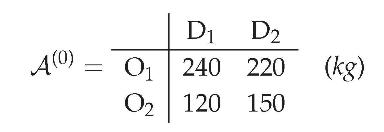

Each entry is one representative pallet weight for that (order, window).

Level 1 (multiset of pallets per cell).Here ${\mathcal{A}}_{ij}^{\left(1\right)}\in \mathcal{M}\left(K\right)$ collects all pallets planned for that cell (multiplicity encodes how many identical pallets). We write multisets as 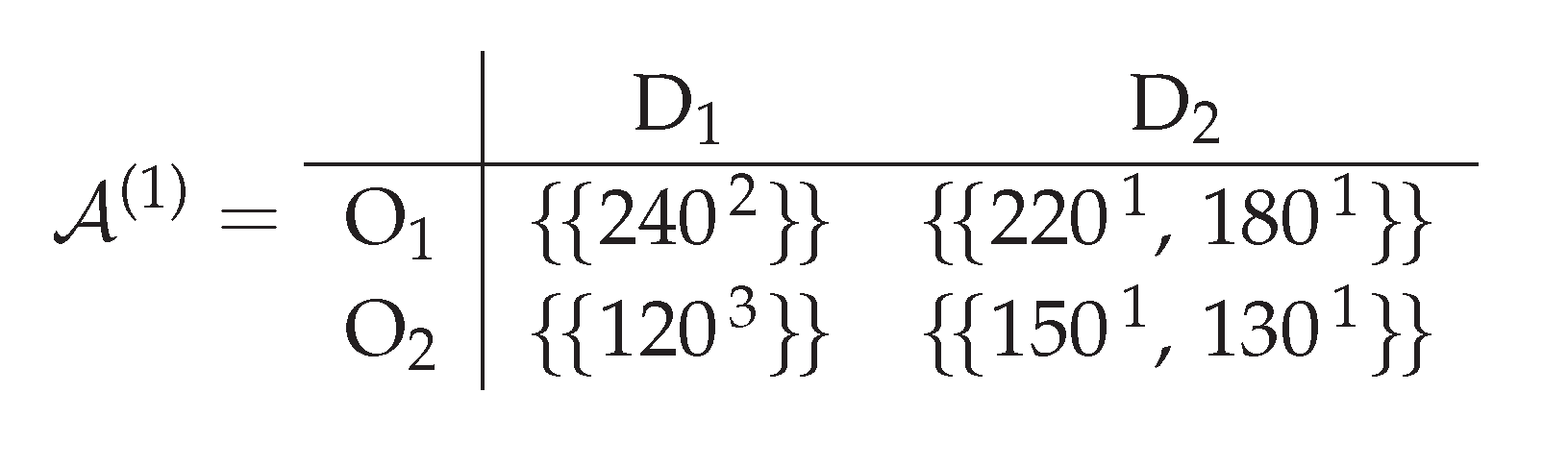$\left\{\{x_1^{k_1},\dots ,x_r^{k_r}\}\right\}$.

Example: ${\mathcal{A}}_{{\mathrm{O}}_1,{\mathrm{D}}_1}^{\left(1\right)}=\left\{\{240,240\}\right\}$ means two identical pallets of 240 kg.

Level 2 (multiset ofload plansper cell).Now ${\mathcal{A}}_{ij}^{\left(2\right)}\in \mathcal{M}\left(\mathcal{M}\left(K\right)\right)$; each element of ${\mathcal{A}}_{ij}^{\left(2\right)}$ is itself a multiset of pallets (i.e., one admissible truckload composition for that cell). For readability, we list the four cells separately:

$$\begin{array}{cc}\hfill {\mathcal{A}}_{{\mathrm{O}}_1,{\mathrm{D}}_1}^{\left(2\right)}& =\left\{\{\underset{\mathrm{plan}\mathrm{A}}{\underbrace{\left\{\left\{{240}^2\right\}\right\}}},\underset{\mathrm{plan}\mathrm{B}}{\underbrace{\left\{\{{180}^2,{100}^1\}\right\}}}\}\right\},\hfill \\ \hfill {\mathcal{A}}_{{\mathrm{O}}_1,{\mathrm{D}}_2}^{\left(2\right)}& =\left\{\{\underset{\mathrm{plan}\mathrm{C}}{\underbrace{\left\{\{{220}^1,{180}^1\}\right\}}},\underset{\mathrm{plan}\mathrm{D}}{\underbrace{\left\{\left\{{200}^2\right\}\right\}}}\}\right\},\hfill \\ \hfill {\mathcal{A}}_{{\mathrm{O}}_2,{\mathrm{D}}_1}^{\left(2\right)}& =\left\{\left\{\underset{\mathrm{plan}\mathrm{E}}{\underbrace{\left\{\left\{{120}^3\right\}\right\}}}\right\}\right\},\hfill \\ \hfill {\mathcal{A}}_{{\mathrm{O}}_2,{\mathrm{D}}_2}^{\left(2\right)}& =\left\{\{\underset{\mathrm{plan}\mathrm{F}}{\underbrace{\left\{\{{150}^1,{130}^1\}\right\}}},\underset{\mathrm{plan}\mathrm{G}}{\underbrace{\left\{\left\{{140}^2\right\}\right\}}}\}\right\}.\hfill \end{array}$$

Interpretation: for $({\mathrm{O}}_1,{\mathrm{D}}_1)$ there are two feasible truckload plans: either two pallets of 240 kg (plan A) or an alternative mix (two pallets of 180 kg plus one of 100 kg, plan B). Thus the level–2 entry is amultiset of admissible pallet-multisets.How levelwise operations act.Given another IMM $\mathcal{B}$ (e.g., a second warehouse), the sum ${(\mathcal{A}\oplus \mathcal{B})}^{\left(0\right)}$ adds scalar weights cellwise; ${(·)}^{\left(1\right)}$ performs the multiset lift of addition on pallet multisets; and ${(·)}^{\left(2\right)}$ combines load plans by the lifted rule on $\mathcal{M}\left(\mathcal{M}\left(K\right)\right)$ (Definition 23). This preserves the three-tier meaning: single pallets → pallet collections → sets of admissible load plans.

Lemma 2  

(Closure per level). For each r, the lifted maps $\widehat{+},\widehat{·}$ and $\widehat{(a\mapsto \lambda a)}$ send ${\left({\mathcal{M}}^r\left(K\right)\right)}^{I\times J}$ to itself, hence the IMM operations are well defined.

Proof. 

Identical to Lemma 1, applied in the universe ${\mathcal{M}}^r\left(K\right)$. □

Theorem 4  

(Iterative MultiMatrix as an Iterative MultiStructure). For each $k\ge 0$, set $H:=K$ and define levelwise multi-operations

$${\#}^{(m,r)}:{\left({\mathcal{M}}^r\left(H\right)\right)}^m⟶{\mathcal{M}}^r\left(H\right),{\#}_{+}^{(2,r)}=\widehat{+},{\#}_{·}^{(2,r)}=\widehat{·},{\#}_{\lambda }^{(1,r)}=\widehat{(a\mapsto \lambda a)}.$$

Then

$${\mathcal{IMS}}_K^{\left(k\right)}:=\left(H,{\left\{{\#}^{(m,r)}\right\}}_{m\in \{1,2\},0\le r\le k}\right)$$

is anIterative MultiStructurein the sense of level-indexed multi-operations. Moreover, the dimensional lift of ${\mathcal{IMS}}_K^{\left(k\right)}$ along $X=I\times J$, acting pointwise at each level r, yields exactly the IMM space of Definition 23.

Proof. 

By construction, each ${\#}^{(m,r)}$ maps m-tuples in ${\mathcal{M}}^r\left(H\right)$ to an element of ${\mathcal{M}}^r\left(H\right)$, so the tuple forms an Iterative MultiStructure. Lifting along X replaces elements by X-indexed arrays and applies the same operations entrywise, which is precisely the IMM definition. □

Theorem 5  

(Reductions: IMM ⇒ MultiMatrix ⇒ Matrix).

• For $k=1$, an IMM is a single matrix with entries in ${\mathcal{M}}^1\left(K\right)=\mathcal{M}\left(K\right)$, with operations from Definition 22; hence IMM generalizes MultiMatrix.
• For $k=0$, an IMM is a classical matrix with entries in ${\mathcal{M}}^0\left(K\right)=K$, and the lifted operations reduce to standard matrix algebra; hence MultiMatrix generalizes classical matrices via the singleton embedding.

Proof. 

(1) Immediate from the definitions with $r=0,1$.

(2) When $r=0$, the lifts $\widehat{+},\widehat{·}$ coincide with $+,·$ on K, and $\widehat{(a\mapsto \lambda a)}$ with scalar multiplication, so we recover ordinary matrix operations. The singleton embedding argument is as in Theorem 3. □

4. Review and Result: MetaMatrix and Iterated MetaMatrix

MetaMatrix is a matrix whose entries are matrices; operations act uniformly by lifting row–column arithmetic to block-level structural composition rules. Iterated MetaMatrix stacks MetaMatrices across levels, forming matrices of matrices of matrices, with operations defined recursively and naturally across depths.

Definition 24  

(Block profile and admissibility). Let $I=\{1,\dots ,p\}$ and $J=\{1,\dots ,q\}$ be finite index sets. Ablock profileon $(I,J)$ consists of two dimension vectors

$$\mathbf{r}={\left(r_i\right)}_{i\in I}\in {\left({\mathbb{N}}_{>0}\right)}^I,\mathbf{s}={\left(s_j\right)}_{j\in J}\in {\left({\mathbb{N}}_{>0}\right)}^J.$$

We say that two profiles $(I,J;\mathbf{r},\mathbf{s})$ and $(J,L;\mathbf{s},\mathbf{t})$ aremultiplication–compatibleif their shared inner dimension vector is identical $(\mathbf{s}$ on both), where $L=\{1,\dots ,\ell \}$ and $\mathbf{t}={\left(t_{\ell }\right)}_{\ell \in L}$.

Definition 25  

(MetaMatrix (matrix of matrices)). Given a block profile $(I,J;\mathbf{r},\mathbf{s})$, aMetaMatrix over Kwith that profile is a function

$$\mathbb{A}:I\times J⟶\underset{(i,j)\in I\times J}{⨆}{K}^{r_i\times s_j},(i,j)⟼A_{ij}\in K^{r_i\times s_j}.$$

If $(I,J;\mathbf{r},\mathbf{s})=(I,J;{\mathbf{r}}^{\prime },{\mathbf{s}}^{\prime })$ we defineblockwise additionandscalar multiplicationentrywise:

$${(\mathbb{A}\oplus \mathbb{B})}_{ij}:=A_{ij}+B_{ij},{(\lambda \odot \mathbb{A})}_{ij}:=\lambda A_{ij}.$$

If $(I,J;\mathbf{r},\mathbf{s})$ and $(J,L;\mathbf{s},\mathbf{t})$ are multiplication–compatible, theMetaMatrix productis

$${(\mathbb{A}\otimes \mathbb{B})}_{i\ell }:=\sum _{j\in J}{A}_{ij}{B}_{j\ell }\in K^{r_i\times t_{\ell }}.$$

Example 17  

(MetaMatrix — hospital staffing (roles × shifts within wards × days)). Fix the ground field $K=\mathbb{N}$ (headcounts). Let rows indexwards$I=\{\mathrm{ICU},\mathrm{GEN}\}$ and columns indexdays$J=\{\mathrm{Mon},\mathrm{Tue}\}$. Each block $A_{ij}\in K^{r_i\times s_j}$ is a $2\times 2$ matrix whose rows are $\{\mathrm{RN},\mathrm{LPN}\}$ (roles) and whose columns are $\{\mathrm{Day},\mathrm{Night}\}$ (shifts). Thus the block profile is $(I,J;\mathbf{r},\mathbf{s})$ with $\mathbf{r}=(2,2)$, $\mathbf{s}=(2,2)$.

Define the MetaMatrix $\ma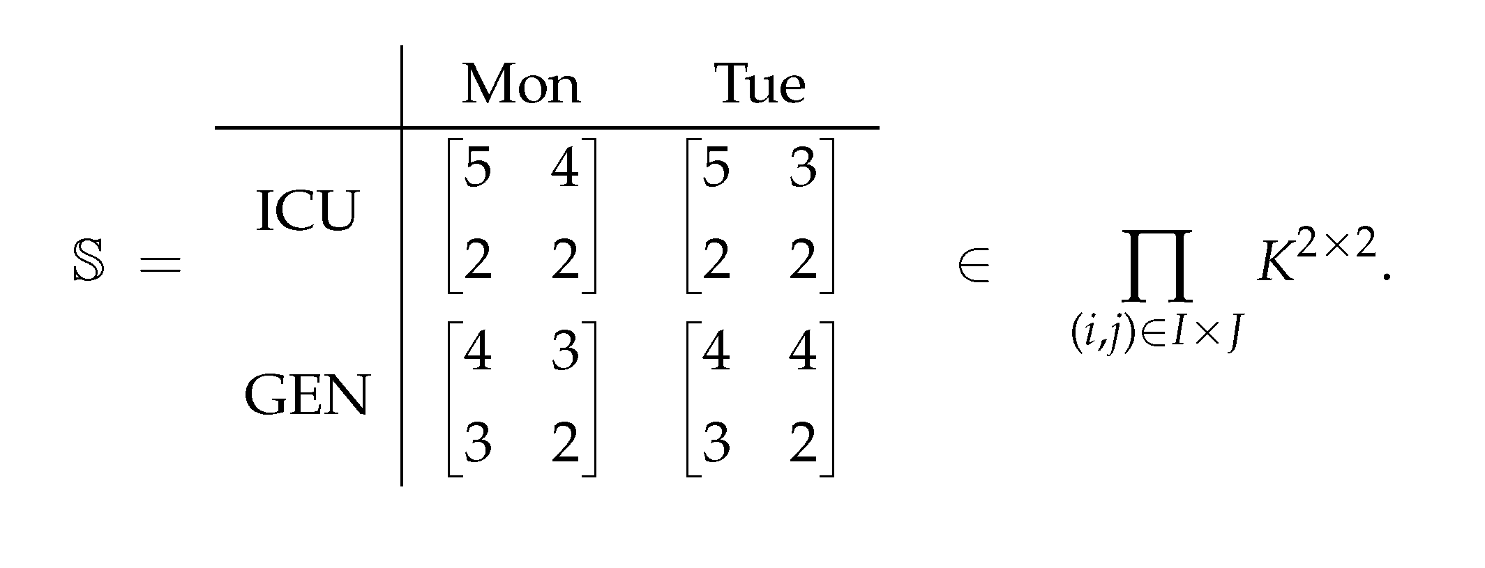thbb{S}:I\times J\to K^{2\times 2}$ by

Its flattening is the $4\times 4$ block–assembled matrix

$$〚\mathbb{S}〛=\begin{array}{cccc}\hfill \mathrm{Mon}\mathrm{Day}& \mathrm{Mon}\mathrm{Night}& \mathrm{Tue}\mathrm{Day}\hfill & \mathrm{Tue}\mathrm{Night}\\ \hfill \begin{array}{c}\hfill 5\end{array}& 4& 5\hfill & 3\\ \hfill 2& 2& 2\hfill & 2\\ \hfill 4& 3& 4\hfill & 4\\ \hfill 3& 2& 3\hfill & 2\end{array}$$

(rows ordered as ICU: RN,ICU:LPN,GEN:RN,GEN:LPN).

Aggregating across shifts. Let ${\mathbb{1}}_{\mathrm{shift}}$ be the block column with profile $(J,\{★\};\mathbf{s},\mathbf{t})$ where $\mathbf{t}=\left(1\right)$ and, for each $j\in J$,

$${\left({\mathbb{1}}_{\mathrm{shift}}\right)}_{j★}:=\left[\begin{array}{c}1\\ 1\end{array}\right]\in K^{2\times 1}.$$

The MetaMatrix product (Definition 25) gives a block column ${(\mathbb{S}\otimes {\mathbb{1}}_{\mathrm{shift}})}_{i★}={\sum }_{j\in J}{A}_{ij}{\left[11\right]}^{\top }\in K^{2\times 1}$. Concretely,

$$\begin{array}{cc}\hfill {(\mathbb{S}\otimes {\mathbb{1}}_{\mathrm{shift}})}_{\mathrm{ICU},★}& =\left[\begin{array}{cc}5& 4\\ 2& 2\end{array}\right]\left[\begin{array}{c}1\\ 1\end{array}\right]+\left[\begin{array}{cc}5& 3\\ 2& 2\end{array}\right]\left[\begin{array}{c}1\\ 1\end{array}\right]=\left[\begin{array}{c}9\\ 4\end{array}\right]+\left[\begin{array}{c}8\\ 4\end{array}\right]=\left[\begin{array}{c}17\\ 8\end{array}\right],\hfill \\ \hfill {(\mathbb{S}\otimes {\mathbb{1}}_{\mathrm{shift}})}_{\mathrm{GEN},★}& =\left[\begin{array}{cc}4& 3\\ 3& 2\end{array}\right]\left[\begin{array}{c}1\\ 1\end{array}\right]+\left[\begin{array}{cc}4& 4\\ 3& 2\end{array}\right]\left[\begin{array}{c}1\\ 1\end{array}\right]=\left[\begin{array}{c}7\\ 5\end{array}\right]+\left[\begin{array}{c}8\\ 5\end{array}\right]=\left[\begin{array}{c}15\\ 10\end{array}\right].\hfill \end{array}$$

Interpretation: over the two days, ICU needs 17 RNs and 8 LPNs in total; the General ward needs 15 RNs and 10 LPNs. The MetaMatrix organizes per–day, per–shift staffing as blocks while allowing standard block algebra for aggregation and downstream costing.

Example 18  

(MetaMatrix — university timetable (periods × rooms within departments × days)). Let $K=\{0,1\}$ (room occupancy). Rows indexdepartments$I=\{\mathrm{Math},\mathrm{CS}\}$ and columns indexdays$J=\{\mathrm{Mon},\mathrm{Tue}\}$. Each block $T_{ij}\in K^{4\times 3}$ encodes a day’s timetable for a department: rows are periods $P=\{1,2,3,4\}$ and columns are rooms $R=\{R_1,R_2,R_3\}$ (1 if the room is used in that period).

Define the MetaMatrix $\ma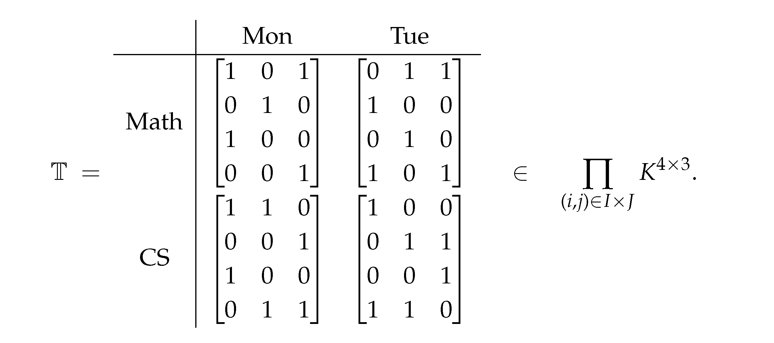thbb{T}:I\times J\to K^{4\times 3}$ by

Its flattening is a $8\times 6$ block–assembled occupancy matrix $〚\mathbb{T}〛$.

From occupancy to seated capacity.Let room capacities be $c\left(R_1\right)=40$, $c\left(R_2\right)=30$, $c\left(R_3\right)=50$ and form the block column $\mathbb{c}$ with profile $(J,\{★\};\mathbf{s},\mathbf{t})$, where $\mathbf{s}=(3,3)$, $\mathbf{t}=\left(1\right)$, and

$${\mathbb{c}}_{j★}:=\left[\begin{array}{c}40\\ 30\\ 50\end{array}\right]\in {\mathbb{R}}^{3\times 1}(j=\mathrm{Mon},\mathrm{Tue}).$$

Then ${(\mathbb{T}\otimes \mathbb{c})}_{i★}={\sum }_{j\in J}{T}_{ij}{\mathbb{c}}_{j★}\in {\mathbb{R}}^{4\times 1}$ returns theseated capacity per periodaccumulated over the two days for department i. For example, for $\mathrm{Math}$ on Monday alone,

$$\left[\begin{array}{ccc}1& 0& 1\\ 0& 1& 0\\ 1& 0& 0\\ 0& 0& 1\end{array}\right]\left[\begin{array}{c}40\\ 30\\ 50\end{array}\right]=\left[\begin{array}{c}90\\ 30\\ 40\\ 50\end{array}\right],$$

so periods 1–4 seat $90,30,40,50$ students respectively. The MetaMatrix organizes each (department, day) timetable as a block, while block multiplication with per–day capacity vectors yields usable aggregates (per–period seat counts) without leaving matrix algebra.

Definition 26  

(Flattening (canonical block assembly)). For a MetaMatrix $\mathbb{A}$ with profile $(I,J;\mathbf{r},\mathbf{s})$ define itsflattening(assembled block matrix)

$$〚\mathbb{A}〛\in K^{\left({\sum }_i{r}_i\right)\times \left({\sum }_j{s}_j\right)}$$

by placing each block $A_{ij}$ in its natural block position; i.e., rows are concatenated in the order $i=1,\dots ,p$ and columns in the order $j=1,\dots ,q$.

Theorem 6  

(Well-definedness and consistency with classical algebra). Let $\mathbb{A},\mathbb{B}$ be MetaMatrices with the same profile $(I,J;\mathbf{r},\mathbf{s})$, and let $\mathbb{C}$ have profile $(J,L;\mathbf{s},\mathbf{t})$ compatible with $\mathbb{A}$. Then

$$〚\mathbb{A}\oplus \mathbb{B}〛=〚\mathbb{A}〛+〚\mathbb{B}〛,〚\lambda \odot \mathbb{A}〛=\lambda 〚\mathbb{A}〛,$$

$$〚\mathbb{A}\otimes \mathbb{C}〛=〚\mathbb{A}〛·〚\mathbb{C}〛.$$

In particular, ⊕, ⊙, and ⊗ are well defined and associative whenever the inner profiles match, and flattening is a homomorphism into the classical matrix algebra.

Proof. 

All identities are standard block–matrix equalities. Each entry of $〚\mathbb{A}\oplus \mathbb{B}〛$ (resp. $\lambda \odot \mathbb{A}$) equals the blockwise sum (resp. scalar multiple), which matches the definition of ⊕ (resp. ⊙). For products, the $(i,\ell )$ block of the classical product equals ${\sum }_j{A}_{ij}{B}_{j\ell }$, which is exactly ${(\mathbb{A}\otimes \mathbb{C})}_{i\ell }$. Associativity and distributivity follow from the classical laws on blocks of compatible sizes. □

Theorem 7  

(MetaMatrix as a MetaStructure; reduction to classical matrices). Let ${\Sigma }_{\mathrm{mat}}$ be the single–sorted signature with function symbols + (binary), · (binary), and ${(\lambda ·)}_{\lambda \in K}$ (unary). For each pair $(r,s)$ let

$${\mathbf{M}}_{r,s}:=\left(K^{r\times s},+,·(\mathrm{defined}\mathrm{when}r=s),{(\lambda ·)}_{\lambda \in K}\right)$$

be the ${\Sigma }_{\mathrm{mat}}$–structure on the carrier $K^{r\times s}$. Fix a profile $(I,J;\mathbf{r},\mathbf{s})$ and define theMetaStructure operation

$${\Phi }_{\oplus }{\left({\mathbf{M}}_{r_i,s_j}\right)}_{(i,j)\in I\times J}:=\left(K^{\left({\sum }_i{r}_i\right)\times \left({\sum }_j{s}_j\right)},+,·,(\lambda ·)\right),$$

with ${\Gamma }_{\oplus }$ assembling the carrier by block–concatenation and ${\Lambda }_{\oplus }^{+}$ prescribing blockwise addition; similarly define ${\Phi }_{·}$ for block multiplication on compatible profiles via the classical block formula. Then:

(a) 

$(U,\{{\Phi }_{\oplus },{\Phi }_{·},{\left({\Phi }_{\lambda }\right)}_{\lambda \in K}\})$ with $U=\{{\mathbf{M}}_{r,s}:r,s\in {\mathbb{N}}_{>0}\}$ is aMetaStructurein the sense of Definition 14.

(b) 

The data of a MetaMatrix $\mathbb{A}$ with profile $(I,J;\mathbf{r},\mathbf{s})$ is precisely the input tuple to ${\Phi }_{\oplus }$, and $〚\mathbb{A}〛$ is the carrier produced by ${\Gamma }_{\oplus }$. The operations ⊕, ⊙, ⊗ coincide with the meta-operations induced on that carrier.

(c) 

If $r_i=s_j=1$ for all $i,j$, then every block is $1\times 1$ and a MetaMatrix is exactly a classical matrix in $K^{p\times q}$. Thus MetaMatrixgeneralizesclassical matrices.

Proof. 

(a) Uniform carrier constructor $\Gamma$ and symbol–constructors $\Lambda$ are given by block assembly and the standard block formulas; naturality (isomorphism–invariance) is immediate from the functorial behavior of direct sums and products of vector spaces. (b) Unwinding the definitions shows that the meta-operations act blockwise exactly as in Definitions 25–26. (c) With $1\times 1$ blocks, $〚·〛$ is the identity identification of entries with scalars, so we recover ordinary matrices and operations. □

Definition 27  

(Depth, uniform profiles, and recursive objects). Fix adepth$t\in \mathbb{N}$ and, for each level $u=1,\dots ,t$, fix a profile $(I_u,J_u;{\mathbf{r}}^{\left(u\right)},{\mathbf{s}}^{\left(u\right)})$. Adepth–0 Iterated MetaMatrixis a classical matrix $A^{\left(0\right)}\in K^{r\times s}$ (some $r,s$). Recursively, adepth–u Iterated MetaMatrix${\mathbb{A}}^{\left(u\right)}$ is a MetaMatrix with profile $(I_u,J_u;{\mathbf{r}}^{\left(u\right)},{\mathbf{s}}^{\left(u\right)})$ whose entries are depth–$(u-1)$ Iterated MetaMatrices, all using the same level–$(u-1)$ profile.

Example 19  

(Iterated MetaMatrix—regional advertising spend (Regions → Stores → Channels × DayTypes)). We build a depth-2 Iterated MetaMatrix as in Definition 27.

Level 0 (classical matrices).Rows arechannels$C=\{\mathrm{Online},\mathrm{InStore}\}$ and columns areday types$D=\{\mathrm{Weekday},\mathrm{Weekend}\}$. An entry records the (weekly) spend in USD. For a fixed store $\mathrm{S}$ and week $\mathrm{W}$, a block is

$$B_{\mathrm{S},\mathrm{W}}^{\left(0\right)}=\left[\begin{array}{cc}\mathit{Online}/\mathit{Weekday}& \mathit{Online}/\mathit{Weekend}\\ \mathit{InStore}/\mathit{Weekday}& \mathit{InStore}/\mathit{Weekend}\end{array}\right]\in {\mathbb{R}}_{\ge 0}^{2\times 2}.$$

Level 1 (MetaMatrix: Stores×Weeks). Let $I_1=\{\mathrm{S}1,\mathrm{S}2\}$ (stores), $J_1=\{\mathrm{W}1,\mathrm{W}2\}$ (weeks), and ${\mathbf{r}}^{\left(1\right)}=(2,2)$, ${\mathbf{s}}^{\left(1\right)}=(2,2)$ (each block $2\times 2$). For the (Region,Month)$=(\mathrm{East},\mathrm{Jan})$ cell we specify the four level-0 blocks:

$${\mathbb{A}}_{\mathrm{East},\mathrm{Jan}}^{\left(1\right)}(i,j)=B_{i,j}^{\left(0\right)}\mathrm{with}\begin{array}{c}{B}_{\mathrm{S}1,\mathrm{W}1}^{\left(0\right)}=\left[\begin{array}{cc}300& 500\\ 200& 400\end{array}\right],B_{\mathrm{S}1,\mathrm{W}2}^{\left(0\right)}=\left[\begin{array}{cc}320& 480\\ 220& 380\end{array}\right],\hfill \\ B_{\mathrm{S}2,\mathrm{W}1}^{\left(0\right)}=\left[\begin{array}{cc}250& 450\\ 180& 350\end{array}\right],B_{\mathrm{S}2,\mathrm{W}2}^{\left(0\right)}=\left[\begin{array}{cc}260& 440\\ 190& 360\end{array}\right].\hfill \end{array}$$

Level 2 (MetaMatrix: Regions×Months). Let $I_2=\{\mathrm{East},\mathrm{West}\}$ and $J_2=\{\mathrm{Jan},\mathrm{Feb}\}$ with ${\mathbf{r}}^{\left(2\right)}=(2,2)$, ${\mathbf{s}}^{\left(2\right)}=(2,2)$, so each entry is a level-1 MetaMatrix as above. Thus ${\mathbb{A}}^{\left(2\right)}:I_2\times J_2\to {\mathrm{MetaMat}}_{(I_1,J_1;{\mathbf{r}}^{\left(1\right)},{\mathbf{s}}^{\left(1\right)})}$.

Nested aggregation via MetaMatrix products. Let $d:=\left[\begin{array}{c}1\\ 1\end{array}\right]\in {\mathbb{R}}^{2\times 1}$ (sum Weekday+Weekend). At level 1 define the block column ${\mathbb{d}}^{\left(1\right)}:J_1\times \{★\}\to {\mathbb{R}}^{2\times 1}$ by ${\left({\mathbb{d}}^{\left(1\right)}\right)}_{j★}=d$ for each $j\in J_1$. Then the level-1 product

$${\left({\mathbb{A}}_{\mathrm{East},\mathrm{Jan}}^{\left(1\right)}\otimes {\mathbb{d}}^{\left(1\right)}\right)}_{i★}=\sum _{j\in J_1}{B}_{i,j}^{\left(0\right)}d\in {\mathbb{R}}^{2\times 1}$$

returns, for each store i, thetwo-channel weekly totals summed over weeks. Compute explicitly:

Store $\mathrm{S}1$.

$$B_{\mathrm{S}1,\mathrm{W}1}^{\left(0\right)}d=\left[\begin{array}{c}300+500\\ 200+400\end{array}\right]=\left[\begin{array}{c}800\\ 600\end{array}\right],B_{\mathrm{S}1,\mathrm{W}2}^{\left(0\right)}d=\left[\begin{array}{c}320+480\\ 220+380\end{array}\right]=\left[\begin{array}{c}800\\ 600\end{array}\right],$$

$$\Rightarrow \sum _j{B}_{\mathrm{S}1,j}^{\left(0\right)}d=\left[\begin{array}{c}1600\\ 1200\end{array}\right].$$

Store $\mathrm{S}2$.

$$B_{\mathrm{S}2,\mathrm{W}1}^{\left(0\right)}d=\left[\begin{array}{c}700\\ 530\end{array}\right],B_{\mathrm{S}2,\mathrm{W}2}^{\left(0\right)}d=\left[\begin{array}{c}700\\ 550\end{array}\right],\Rightarrow \sum _j{B}_{\mathrm{S}2,j}^{\left(0\right)}d=\left[\begin{array}{c}1400\\ 1080\end{array}\right].$$

Now sum channels by ${\rho }^{\top }:=\left[11\right]$ to obtain per-store monthly totals:

$$\mathrm{S}1:{\rho }^{\top }\left[\begin{array}{c}1600\\ 1200\end{array}\right]=2800,\mathrm{S}2:{\rho }^{\top }\left[\begin{array}{c}1400\\ 1080\end{array}\right]=2480.$$

Finally, sum stores (scalar addition) to get the East–Jan regional total:

$$\mathrm{East}--\mathrm{Jan}\mathrm{monthly}\mathrm{spend}=2800+2480=5280\mathrm{USD}.$$

(The same construction, applied one level higher as ${\mathbb{A}}^{\left(2\right)}\otimes {\mathbb{d}}^{\left(2\right)}$ with ${\left({\mathbb{d}}^{\left(2\right)}\right)}_{j★}=d$, executes the week-summing step uniformlyinsideeach level-1 block, illustrating the recursive nature.)

Example 20  

(Iterated MetaMatrix — manufacturing throughput (Regions → Plants → Lines×Days with Stations×Shifts blocks)). We construct a depth-2 Iterated MetaMatrix capturing production counts.

Level 0 (Stations×Shifts). For each line/day, let rows beshifts$S=\{\mathrm{Day},\mathrm{Night}\}$ and columns bestations$R=\{\mathrm{A},\mathrm{B}\}$. An entry is the number of finished units. Thus a block $P_{\mathrm{Line},\mathrm{Day}}^{\left(0\right)}\in {\mathbb{N}}^{2\times 2}$.

Level 1 (MetaMatrix: Lines×Days). Fix lines $I_1=\{\mathrm{L}1,\mathrm{L}2\}$ and days $J_1=\{\mathrm{Mon},\mathrm{Tue}\}$ with ${\mathbf{r}}^{\left(1\right)}={\mathbf{s}}^{\left(1\right)}=(2,2)$ (each block $2\times 2$). ForPlant Northwe set:

$$\begin{array}{c}{P}_{\mathrm{L}1,\mathrm{Mon}}^{\left(0\right)}=\left[\begin{array}{cc}12& 8\\ 9& 7\end{array}\right],P_{\mathrm{L}1,\mathrm{Tue}}^{\left(0\right)}=\left[\begin{array}{cc}10& 9\\ 8& 8\end{array}\right],\hfill \\ P_{\mathrm{L}2,\mathrm{Mon}}^{\left(0\right)}=\left[\begin{array}{cc}11& 7\\ 8& 6\end{array}\right],P_{\mathrm{L}2,\mathrm{Tue}}^{\left(0\right)}=\left[\begin{array}{cc}9& 8\\ 7& 7\end{array}\right].\hfill \end{array}$$

ForPlant Southwe set:

$$\begin{array}{c}{P}_{\mathrm{L}1,\mathrm{Mon}}^{\left(0\right)}=\left[\begin{array}{cc}13& 7\\ 9& 8\end{array}\right],P_{\mathrm{L}1,\mathrm{Tue}}^{\left(0\right)}=\left[\begin{array}{cc}12& 8\\ 9& 7\end{array}\right],\hfill \\ P_{\mathrm{L}2,\mathrm{Mon}}^{\left(0\right)}=\left[\begin{array}{cc}10& 9\\ 7& 6\end{array}\right],P_{\mathrm{L}2,\mathrm{Tue}}^{\left(0\right)}=\left[\begin{array}{cc}11& 7\\ 8& 7\end{array}\right].\hfill \end{array}$$

Each plant thereby determines a level-1 MetaMatrix ${\mathbb{P}}_{\mathrm{Plant}}^{\left(1\right)}$ on $(I_1,J_1)$.

Level 2 (MetaMatrix: Regions×Weeks).  Let regions $I_2=\{\mathrm{North},\mathrm{South}\}$, weeks $J_2=\left\{\mathrm{W}1\right\}$, and profile ${\mathbf{r}}^{\left(2\right)}={\mathbf{s}}^{\left(2\right)}=\left(2\right)$ so that each $(\mathrm{Region},\mathrm{W}1)$ entry is the corresponding level-1 ${\mathbb{P}}_{\mathrm{Plant}}^{\left(1\right)}$.

Nested aggregation (units per week). Let $e:=\left[\begin{array}{c}1\\ 1\end{array}\right]$ to sum stations, and ${\rho }^{\top }:=\left[11\right]$ to sum shifts. At level 1 define ${\left({\mathbb{e}}^{\left(1\right)}\right)}_{j★}=e$ for $j\in J_1$. Then, for any line i,

$${\left({\mathbb{P}}_{\mathrm{Plant}}^{\left(1\right)}\otimes {\mathbb{e}}^{\left(1\right)}\right)}_{i★}=\sum _{j\in J_1}{P}_{i,j}^{\left(0\right)}e\in {\mathbb{N}}^{2\times 1}(\mathit{per}-\mathit{shift}\mathit{totals},\mathit{summed}\mathit{over}\mathit{days}).$$

Apply ${\rho }^{\top }$ to obtain the line’s two-day total. Compute explicitly:

Plant North.

$$\begin{array}{c}\mathrm{L}1:P_{\mathrm{L}1,\mathrm{Mon}}^{\left(0\right)}e=\left[\begin{array}{c}20\\ 16\end{array}\right],P_{\mathrm{L}1,\mathrm{Tue}}^{\left(0\right)}e=\left[\begin{array}{c}19\\ 16\end{array}\right]\Rightarrow {\rho }^{\top }(·)=36+35=71,\hfill \\ \mathrm{L}2:P_{\mathrm{L}2,\mathrm{Mon}}^{\left(0\right)}e=\left[\begin{array}{c}18\\ 14\end{array}\right],P_{\mathrm{L}2,\mathrm{Tue}}^{\left(0\right)}e=\left[\begin{array}{c}17\\ 14\end{array}\right]\Rightarrow {\rho }^{\top }(·)=32+31=63.\hfill \end{array}$$

Plant North weekly total: $71+63=134$ units.

Plant South.

$$\begin{array}{c}\mathrm{L}1:P_{\mathrm{L}1,\mathrm{Mon}}^{\left(0\right)}e=\left[\begin{array}{c}20\\ 17\end{array}\right],P_{\mathrm{L}1,\mathrm{Tue}}^{\left(0\right)}e=\left[\begin{array}{c}20\\ 16\end{array}\right]\Rightarrow {\rho }^{\top }(·)=37+36=73,\hfill \\ \mathrm{L}2:P_{\mathrm{L}2,\mathrm{Mon}}^{\left(0\right)}e=\left[\begin{array}{c}19\\ 13\end{array}\right],P_{\mathrm{L}2,\mathrm{Tue}}^{\left(0\right)}e=\left[\begin{array}{c}18\\ 15\end{array}\right]\Rightarrow {\rho }^{\top }(·)=32+33=65.\hfill \end{array}$$

Plant South weekly total: $73+65=138$ units.

Regional aggregation (level 2).Placing ${\mathbb{P}}_{\mathrm{North}}^{\left(1\right)}$ and ${\mathbb{P}}_{\mathrm{South}}^{\left(1\right)}$ as the two blocks of ${\mathbb{P}}^{\left(2\right)}$ (rows $I_2$, single column $J_2$) exposes a final summation across plants as a level-2 operation (scalar addition of the computed plant totals), yielding the region vector

$$\left[\begin{array}{c}\mathit{North}\\ \mathit{South}\end{array}\right]=\left[\begin{array}{c}134\\ 138\end{array}\right].$$

This example illustrates how the same block recipe (“sum columns by e, then sum rows by ${\rho }^{\top }$, then sum over days”) is reused recursively inside each entry of the next level.

Definition 28  

(Recursive flattening and operations). Define theflattening$〚·{〛}^{\downarrow u}$ by

$$〚A^{\left(0\right)}{〛}^{\downarrow 0}:=A^{\left(0\right)},〚{\mathbb{A}}^{\left(u\right)}{〛}^{\downarrow u}:=〚{\left(〚A_{ij}^{(u-1)}{〛}^{\downarrow (u-1)}\right)}_{(i,j)\in I_u\times J_u}〛,$$

i.e., first flatten each entry to a classical block, then assemble the block matrix. Define ⊕, ⊙, and ⊗ on depth–u objects entrywise at level u using the MetaMatrix rules, assuming inner profiles match.

Theorem 8  

(Flattening is a homomorphism at every depth). For each depth $u\ge 0$ and all well–typed ${\mathbb{A}}^{\left(u\right)},{\mathbb{B}}^{\left(u\right)}$ and scalars λ,

$$〚{\mathbb{A}}^{\left(u\right)}\oplus {\mathbb{B}}^{\left(u\right)}{〛}^{\downarrow u}=〚{\mathbb{A}}^{\left(u\right)}{〛}^{\downarrow u}+〚{\mathbb{B}}^{\left(u\right)}{〛}^{\downarrow u},〚\lambda \odot {\mathbb{A}}^{\left(u\right)}{〛}^{\downarrow u}=\lambda 〚{\mathbb{A}}^{\left(u\right)}{〛}^{\downarrow u},$$

$$〚{\mathbb{A}}^{\left(u\right)}\otimes {\mathbb{B}}^{\left(u\right)}{〛}^{\downarrow u}=〚{\mathbb{A}}^{\left(u\right)}{〛}^{\downarrow u}·〚{\mathbb{B}}^{\left(u\right)}{〛}^{\downarrow u}.$$

Proof. 

Induction on u. The base $u=0$ is trivial. For $u\to u+1$, apply the induction hypothesis to each entry (depth u), then Theorem 6 at the top MetaMatrix level to assemble blocks; the three identities follow. □

Theorem 9  

(Iterated MetaMatrix as an Iterated MetaStructure; reductions). For each level u let $U^{\left(u\right)}$ be the class of depth–u Iterated MetaMatrices with fixed profile $(I_u,J_u;{\mathbf{r}}^{\left(u\right)},{\mathbf{s}}^{\left(u\right)})$. The triple

$${\mathfrak{M}}^{\left(u\right)}:=\left(U^{\left(u\right)},{\Phi }_{\oplus }^{\left(u\right)},{\Phi }_{·}^{\left(u\right)},{\left({\Phi }_{\lambda }^{\left(u\right)}\right)}_{\lambda \in K}\right),$$

where ${\Phi }^{\left(u\right)}$ applies the MetaMatrix constructors to entries in $U^{(u-1)}$ and then assembles via Γ (Definition 14), is anIterated MetaStructure. Moreover:

(a) 

(Generalization) Depth 1 recovers MetaMatrix; depth 0 recovers classical matrices.

(b) 

(Compatibility) The flattening $〚·{〛}^{\downarrow u}$ is a natural homomorphism ${\mathfrak{M}}^{\left(u\right)}\to K$–Mat(Theorem 8).

Proof. 

The carrier constructors $\Gamma$ and symbol–constructors $\Lambda$ are given uniformly at each depth by the block assembly of Definition 28 and the block rules of Definition 25. Naturality is inherited from the functoriality of assembling direct sums/products of vector spaces. (a) follows from the definitions; (b) is Theorem 8. □

5. Conclusions

In this paper we defined HyperMatrix, SuperHyperMatrix, MultiMatrix, Iterative MultiMatrix, MetaMatrix, and Iterated MetaMatrix—all as extensions of the classical notion of a matrix—and we offer a concise examination of their properties. In future work, we plan to consider extensions that incorporate uncertainty and multi-valuedness by employing advanced set-theoretic frameworks such as the Fuzzy Set [49,50,51,52], Intuitionistic Fuzzy Set [53,54], Vague Sets [55,56,57], Hesitant Fuzzy Set [58,59,60], Picture Fuzzy Set [61,62,63], Neutrosophic Set [64,65,66], and Plithogenic Set [67,68,69,70].

References

- Smarandache, F. Foundation of SuperHyperStructure & Neutrosophic SuperHyperStructure. Neutrosophic Sets and Systems 2024, 63, 21. [Google Scholar]
- Al-Tahan, M.; Davvaz, B.; Smarandache, F.; Anis, O. On some neutroHyperstructures. Symmetry 2021, 13, 535. [Google Scholar] [CrossRef]
- Davvaz, B.; Nezhad, A.D.; Nejad, S.M. Algebraic hyperstructure of observable elementary particles including the Higgs boson. Proceedings of the National Academy of Sciences, India Section A: Physical Sciences 2020, 90, 169–176. [Google Scholar] [CrossRef]
- Ruggero, M.S.; Vougiouklis, T. Hyperstructures in Lie-Santilli admissibility and iso-theories. Ratio Mathematica 2017, 33, 151. [Google Scholar]
- Das, A.K.; Das, R.; Das, S.; Debnath, B.K.; Granados, C.; Shil, B.; Das, R. A Comprehensive Study of Neutrosophic SuperHyper BCI-Semigroups and their Algebraic Significance. Transactions on Fuzzy Sets and Systems 2025, 8, 80. [Google Scholar]
- Rahmati, M.; Hamidi, M. Extension of g-algebras to superhyper g-algebras. Neutrosophic Sets and Systems 2023, 55, 557–567. [Google Scholar]
- Fujita, T. Weak HyperFuzzy Set and Weak SuperHyperFuzzy Set. Computational Methods 2025, 2, 11–26. [Google Scholar]
- Kong, X. Students’ Innovation Ability Evaluation in Vocational Colleges Based on the STEAM Education Concept: A Neutrosophic SuperHyper Pentapartitioned Process Model. Neutrosophic Sets and Systems 2025, 93, 250–261. [Google Scholar]
- Fujita, T. Medical SuperHyperStructure and Healthcare SuperHyperStructure. Journal of Medicine and Health Research 2025, 10, 243–262. [Google Scholar] [CrossRef]
- Li, Y. A Neutrosophic SuperHyperModal Framework for the Multilayered Evaluation of New Media Marketing Strategies in the Automotive Industry. Neutrosophic Sets and Systems 2025, 88, 28. [Google Scholar]
- Jech, T. Set theory: The third millennium edition, revised and expanded; Springer, 2003.
- Smarandache, F. SuperHyperFunction, SuperHyperStructure, Neutrosophic SuperHyperFunction and Neutrosophic SuperHyperStructure: Current understanding and future directions; Infinite Study, 2023.
- Smarandache, F. Introduction to SuperHyperAlgebra and Neutrosophic SuperHyperAlgebra. Journal of Algebraic Hyperstructures and Logical Algebras 2022. [Google Scholar]
- Fujita, T.; Smarandache, F. A Unified Framework for U-Structures and Functorial Structure: Managing Super, Hyper, SuperHyper, Tree, and Forest Uncertain Over/Under/Off Models. Neutrosophic Sets and Systems 2025, 91, 337–380. [Google Scholar]
- Selvachandran, G.; Salleh, A.R. Hypergroup theory applied to fuzzy soft sets. Global Journal of Pure and Applied Sciences 2015, 11, 825–834. [Google Scholar]
- Stenstrom, B. Rings of quotients: an introduction to methods of ring theory; Vol. 217, Springer Science & Business Media, 2012.
- Jun, Y.B.; Park, C.H.; Alshehri, N.O. Hypervector spaces based on intersectional soft sets. In Proceedings of the Abstract and Applied Analysis. Wiley Online Library, Vol. 2014; p. 784523. [Google Scholar]
- Tallini, M.S. Hypervector spaces. In Proceedings of the Proceeding of the 4th International Congress in Algebraic Hyperstructures and Applications; 1991; pp. 167–174. [Google Scholar]
- Gross, J.L.; Yellen, J.; Anderson, M. Graph theory and its applications; Chapman and Hall/CRC, 2018.
- Diestel, R. Graph theory 3rd ed. Graduate texts in mathematics 2005, 173, 12. [Google Scholar]
- Diestel, R. Graph theory; Springer (print edition); Reinhard Diestel (eBooks), 2024.
- Vougioukli, S. Helix hyperoperation in teaching research. Science & Philosophy 2020, 8, 157–163. [Google Scholar]
- Vougioukli, S. Hyperoperations defined on sets of S -helix matrices. 2020.
- Rezaei, A.; Smarandache, F.; Mirvakili, S. Applications of (Neutro/Anti)sophications to Semihypergroups. Journal of Mathematics 2021. [Google Scholar] [CrossRef]
- Vougioukli, S. HELIX-HYPEROPERATIONS ON LIE-SANTILLI ADMISSIBILITY. Algebras Groups and Geometries 2023. [Google Scholar] [CrossRef]
- Corsini, P.; Leoreanu, V. Applications of hyperstructure theory; Vol. 5, Springer Science & Business Media, 2013.
- Novák, M.; Křehlík, Š.; Ovaliadis, K. Elements of hyperstructure theory in UWSN design and data aggregation. Symmetry 2019, 11, 734. [Google Scholar] [CrossRef]
- Oguz, G.; Davvaz, B. Soft topological hyperstructure. J. Intell. Fuzzy Syst. 2021, 40, 8755–8764. [Google Scholar] [CrossRef]
- Smarandache, F. SuperHyperStructure & Neutrosophic SuperHyperStructure, 2024. Accessed: 2024-12-01.
- Shinoj, T.; John, S.J. Intuitionistic fuzzy multisets and its application in medical diagnosis. World academy of science, engineering and technology 2012, 6, 1418–1421. [Google Scholar]
- Ejegwa, P. New operations on intuitionistic fuzzy multisets. Journal of Mathematics and Informatics 2015, 3, 17–23. [Google Scholar]
- Girish, K.; John, S.J. Rough Multisets and Information Multisystems. Advances in Decision sciences 2011. [Google Scholar] [CrossRef]
- Girish, K.; John, S.J. On rough multiset relations. International Journal of Granular Computing, Rough Sets and Intelligent Systems 2014, 3, 306–326. [Google Scholar] [CrossRef]
- Fujita, T. Iterative Multistructure and Curried Iterative Multistructure: Graph, Function, Chemical Structure, and beyond 2025.
- Fujita, T. Introduction for Structure, HyperStructure, SuperHyperStructure, MultiStructure, Iterative MultiStructure, TreeStructure, and ForestStructure 2025.
- Fujita, T. MetaStructure, Meta-HyperStructure, and Meta-SuperHyperStructure, 2025. [CrossRef]
- Fujita, T. MetaHyperGraphs, MetaSuperHyperGraphs, and Iterated MetaGraphs: Modeling Graphs of Graphs, Hypergraphs of Hypergraphs, Superhypergraphs of Superhypergraphs, and Beyond, 2025. [CrossRef]
- Horn, R.A.; Johnson, C.R. Matrix analysis. 1985.
- Yaz, E.E. Linear Matrix Inequalities In System And Control Theory. Proceedings of the IEEE 1998, 86, 2473–2474. [Google Scholar] [CrossRef]
- Golub, G.H. Matrix computations. 1983.
- Chrzeszczyk, A.; Kochanowski, J. Matrix Computations. In Proceedings of the Encyclopedia of Parallel Computing; 2011. [Google Scholar]
- Wu, F.; Zhang, T.; de Souza, A.H.; Fifty, C.; Yu, T.; Weinberger, K.Q. Simplifying Graph Convolutional Networks. In Proceedings of the International Conference on Machine Learning; 2019. [Google Scholar]
- Lee, D.D.; Sebastian, H.; y, S. Algorithms for Non-negative Matrix Factorization. In Proceedings of the Neural Information Processing Systems; 2000. [Google Scholar]
- Engler, A.J.; Engler, A.J.; Sen, S.; Sen, S.; Sweeney, H.L.; Discher, D.E. Matrix Elasticity Directs Stem Cell Lineage Specification. Cell 2006, 126, 677–689. [Google Scholar] [CrossRef]
- Motameni, M.; Ameri, R.; Sadeghi, R. Hypermatrix Based on Krasner Hypervector Spaces. 2013.
- Fujita, T. A theoretical exploration of hyperconcepts: Hyperfunctions, hyperrandomness, hyperdecision-making, and beyond (including a survey of hyperstructures). Advancing Uncertain Combinatorics through Graphization, Hyperization, and Uncertainization: Fuzzy, Neutrosophic, Soft, Rough, and Beyond 2025, p. 111.
- Tropp, J.A. Tropp, J.A. An Introduction to Matrix Concentration Inequalities. ArXiv 2015, abs/1501.01571.
- Bellman, R. Introduction to Matrix Analysis. 1972.
- Zadeh, L.A. Fuzzy sets. Information and control 1965, 8, 338–353. [Google Scholar] [CrossRef]
- Akram, M.; Luqman, A. Fuzzy hypergraphs and related extensions; Springer, 2020.
- Al-Hawary, T. Complete fuzzy graphs. International Journal of Mathematical Combinatorics 2011, 4, 26. [Google Scholar]
- Nishad, T.; Al-Hawary, T.A.; Harif, B.M. General Fuzzy Graphs. Ratio Mathematica 2023, 47. [Google Scholar]
- Atanassov, K.T. Circular intuitionistic fuzzy sets. Journal of Intelligent & Fuzzy Systems 2020, 39, 5981–5986. [Google Scholar] [CrossRef]
- Atanassov, K.T.; Gargov, G. Intuitionistic fuzzy logics; Springer, 2017.
- Lu, A.; Ng, W. Vague sets or intuitionistic fuzzy sets for handling vague data: which one is better? In Proceedings of the International conference on conceptual modeling. Springer; 2005; pp. 401–416. [Google Scholar]
- Gau, W.L.; Buehrer, D.J. Vague sets. IEEE transactions on systems, man, and cybernetics 1993, 23, 610–614. [Google Scholar] [CrossRef]
- Bustince, H.; Burillo, P. Vague sets are intuitionistic fuzzy sets. Fuzzy sets and systems 1996, 79, 403–405. [Google Scholar]
- Torra, V.; Narukawa, Y. On hesitant fuzzy sets and decision. In Proceedings of the 2009 IEEE international conference on fuzzy systems. IEEE; 2009; pp. 1378–1382. [Google Scholar]
- Torra, V. Hesitant fuzzy sets. International journal of intelligent systems 2010, 25, 529–539. [Google Scholar]
- Xu, Z. Hesitant fuzzy sets theory; Vol. 314, Springer, 2014.
- Das, S.; Ghorai, G.; Pal, M. Picture fuzzy tolerance graphs with application. Complex & Intelligent Systems 2022, 8, 541–554. [Google Scholar]
- Khan, W.A.; Arif, W.; NGUYEN, Q.H.; Le, T.T.; Van Pham, H. Picture Fuzzy Directed Hypergraphs with applications towards decision-making and managing hazardous chemicals. IEEE Access 2024. [Google Scholar]
- Cuong, B.C.; Kreinovich, V. Picture fuzzy sets-a new concept for computational intelligence problems. In Proceedings of the 2013 third world congress on information and communication technologies (WICT 2013). IEEE; 2013; pp. 1–6. [Google Scholar]
- Smarandache, F.; Jdid, M. An Overview of Neutrosophic and Plithogenic Theories and Applications 2023.
- Broumi, S.; Talea, M.; Bakali, A.; Smarandache, F. Single valued neutrosophic graphs. Journal of New theory 2016, 10, 86–101. [Google Scholar]
- Broumi, S.; Talea, M.; Bakali, A.; Smarandache, F.; Kumar, P.K. Shortest path problem on single valued neutrosophic graphs. In Proceedings of the 2017 international symposium on networks, computers and communications (ISNCC). IEEE; 2017; pp. 1–6. [Google Scholar]
- Sultana, F.; Gulistan, M.; Ali, M.; Yaqoob, N.; Khan, M.; Rashid, T.; Ahmed, T. A study of plithogenic graphs: applications in spreading coronavirus disease (COVID-19) globally. Journal of ambient intelligence and humanized computing 2023, 14, 13139–13159. [Google Scholar] [CrossRef]
- Kandasamy, W.V.; Ilanthenral, K.; Smarandache, F. Plithogenic Graphs; Infinite Study, 2020.
- Sathya, P.; Martin, N.; Smarandache, F. Plithogenic Forest Hypersoft Sets in Plithogenic Contradiction Based Multi-Criteria Decision Making. Neutrosophic Sets and Systems 2024, 73, 668–693. [Google Scholar]
- Smarandache, F. Extension of HyperGraph to n-SuperHyperGraph and to Plithogenic n-SuperHyperGraph, and Extension of HyperAlgebra to n-ary (Classical-/Neutro-/Anti-) HyperAlgebra; Infinite Study, 2020.
Disclaimer/Publisher’s Note: The statements, opinions and data contained in all publications are solely those of the individual author(s) and contributor(s) and not of MDPI and/or the editor(s). MDPI and/or the editor(s) disclaim responsibility for any injury to people or property resulting from any ideas, methods, instructions or products referred to in the content. |
© 2025 by the authors. Licensee MDPI, Basel, Switzerland. This article is an open access article distributed under the terms and conditions of the Creative Commons Attribution (CC BY) license (http://creativecommons.org/licenses/by/4.0/).
Copyright: This open access article is published under a Creative Commons CC BY 4.0 license, which permit the free download, distribution, and reuse, provided that the author and preprint are cited in any reuse.