Submitted:
01 October 2025
Posted:
09 October 2025
You are already at the latest version
Abstract
Divisible residuated lattices and MTL-algebras are algebraic structures connected with algebras in t-norm based fuzzy logics, being examples of BLalgebras. They are an important significance in the study of fuzzy logic. The purpose of this paper is to investigate and give classifications of these types of algebras. From computational considerations, we analyze the structure of these residuated lattices of small size n (2 ≤ n ≤ 5) and we give summarizing statistics. To extend these results for higer size, we used computer and a constructive algorithm for generating all residuated lattices.
Keywords:
(divisible) residuated lattice
; MTL-algebra
; ring
1. Introduction
Nonclassical logics have been represented as algebras and they are related to computer science. Residuated lattices were introduced by Dilworth and Ward (see [Di; 38], [WD; 39]) and their study is originated in the context of theory of rings. It is known that the lattice of ideals in a commutative ring is a residuated lattice, see [Bl; 53].
Divisible residuated lattices (or residuated lattice ordered monoids or RL-monoids) and MTL-algebras are two examples of residuated lattices.
Divisible residuated lattices were introduced in [S] as a unifying concept for Heyting algebras and Abelian lattice ordered groups. These residuated lattices satisfying divisibility condition are connected with algebras in t-norm based fuzzy logics, being examples of BL-algebras.
Esteva et al. introduced in [E] the t-norm -based fuzzy logic MTL, to capture the logic of t-norm-based fuzzy logics and their residuum, The resulting algebras are MTL-algebras.
Since BL-algebras are MTL-algebras satisfying divisibility property the question that one can ask is how many residuated lattices satisfy one property and how many satisfy the other.
Properties of MTL-algebras, divisible residuated lattices and a classification of finite residuated lattices can be found in several papers, as for example: [BV; 10], [CFP; 23], [FP; 22], [FP; 23].
In this paper, we present a characterisation for residuated lattices of size and we construct all (up to an isomorphism) divisible residuated lattices and MTL-algebras with elements. Also, we present summarizing statistics. This method can be used to construct finite residuated lattices of larger size, the inconvenience being the large number of algebras that should be generated. This is the reason for which we consider a better idea to use computer. Differences between our approach and the classification given in [BV; 10] are that we give a mathematical proof of such a construction, by using ordinal product, and we provide a constructive algorithm for generating all residuated lattices, which can be easy addapted for higer sizes.
2. Preliminaries
Definition 1 ([Di; 38], [WD; 39]) A (commutative) residuated lattice is an algebra with an order ≤ such that:
(i) is a bounded lattice;
(ii) is a commutative ordered monoid;
(iii) iff for all
If L is a residuated lattice, then we denote for any .
In a residuated lattice L we consider the identities:
Definition 2 ([COM; 09, [CHA; 58], [NL; 03], [I; 09], [T; 99]) A residuated lattice L is called:
(i) an MTL-algebra if L verifies condition;
(ii)divisibleif L verifies condition;
(iii) a BL-algebra if L verifies conditions. A BL-chainis a totally ordered BL-algebra.
(iv) an MV-algebra is a BL-algebra in which for every .
Example 3. 1) For a commutative unitary ring the lattice of ideals is a residuated lattice with the order relation is ⊆ and
for every see [TT; 22]. Moreover, and are ideals of called sum, product, quotient and annihilator, see [BP; 02].
2) If and are two residuated lattices such that and then, the ordinal product (sum) of and is the residuated lattice where
see [I; 09].
3) For we consider the chain organized as lattice by and as bounded residuated lattice with de Fodor’s implication
with the corresponding Fodor’s t-norm
see [F].
3. Main Results
Proposition 4. ( [I; 09]) Let and be residuated lattices.
(i) If and are divisible, then is divisible;
(ii) If and are MTL-algebras and is a chain, then is an MTL-algebra.
Remark 5. 1) If and are BL-algebras and is a chain, then is a BL-algebra.
2) If and are BL-algebras and is not a chain, then is a divisible residuated lattice which is not a BL-algebra, since it is not an MTL-algebra.
In the following, we present some examples of divisible and MTL algebras and an way to obtain its.
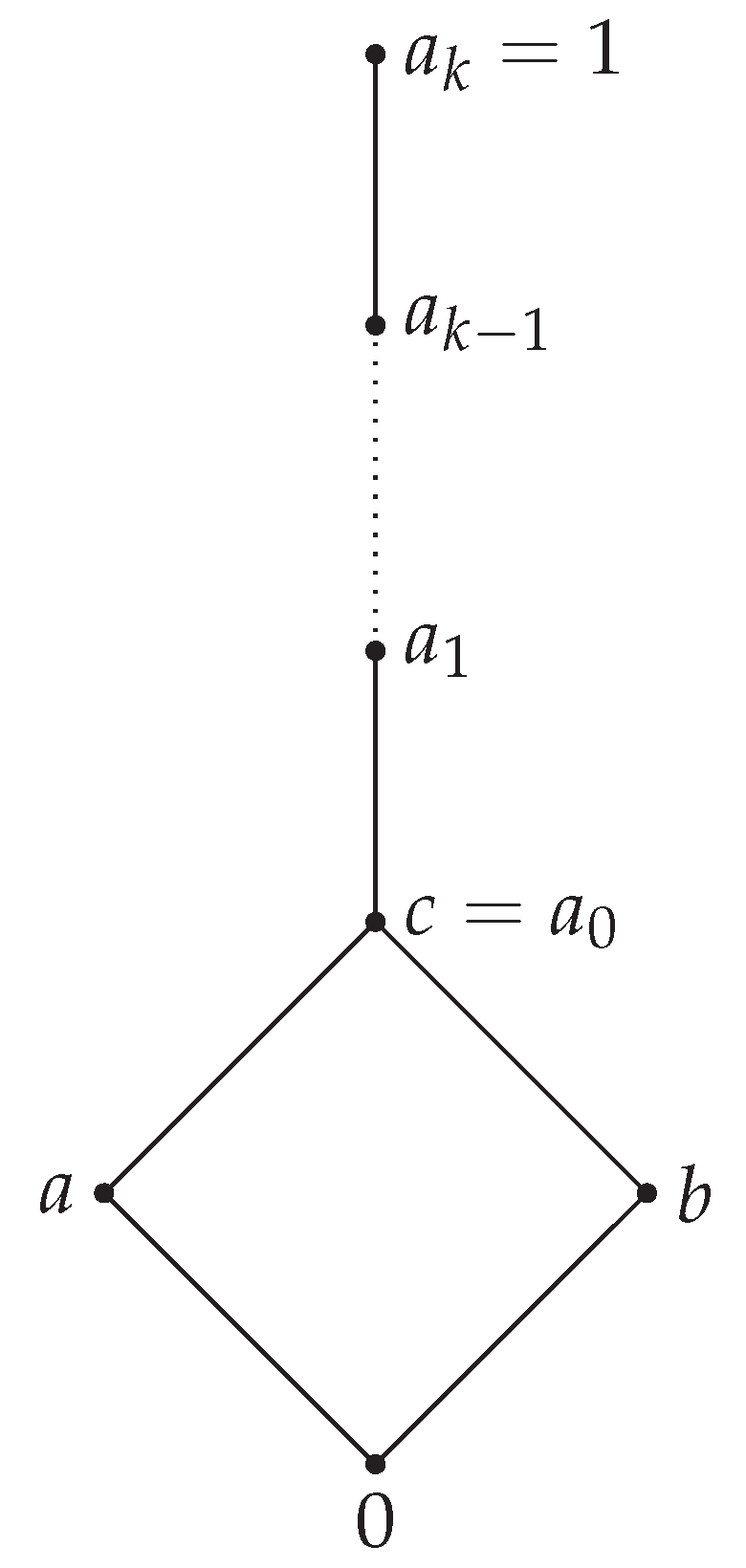
Example 6. To generate a divisible residuated lattice with elements, which is not an MTL-algebra organized as lattice as in Figure 1,
We consider the commutative rings and
For the lattice of ideals is , which is a Boolean algebra so a BL-algebra, with the following operations:
Also, we know that is the only MV-chain (up to an isomorphism) with elements, see [FP; 22], so, it is a BL-chain.
The ring has ideals: ..., and
For every we have
and
We consider two BL-algebras isomorphic with and denoted by and Using Proposition 4, we generate a divisible residuated lattice with elements, for any
This residuated lattice is not an MTL algebra since
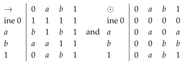
For example, for we obtain a divisible residuated lattice(which is not a MTL algebra) with the following operations:
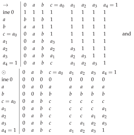
since in , we have
and
so is a BL-algebra with 5 elements with the operations:
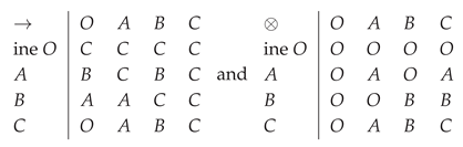
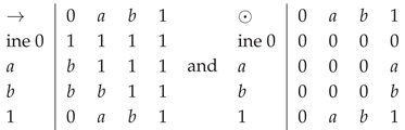
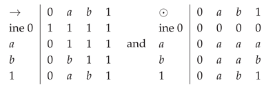
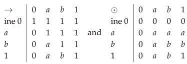
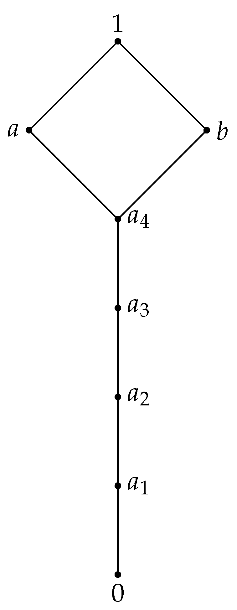
Examples 7. To generate an MTL-algebra with 8 elements (which is not divisible) organized as a lattice as in Figure 2,
we consider the MTL-algebra with the following operations:
 ,
,(see [I; 09], p.218) and BL-algebra isomorphic with
Then is an MTL-algebra, by Proposition 4, with the operations:
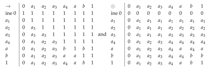 .
.
Remark 8. Let Lbe a residuated lattice with 2 elements. Obviously, with
 .
.Obviously, L is the Boolean algebra thus L has and properties.
Remark 9. Let Lbe a residuated lattice with 3 elements, so Obviously, and L is a chain.
We have the following cases:
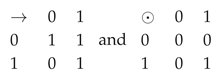
1) Obviously, . If a contradiction.
If we obtain a residuated lattice with the following operations:
 .
.
is a BL-algebra isomorphic with , that is not an MV-algebra.
Obviously, satisfies + properties.
If a contradiction.
2) In this case, , so, .
If we obtain a residuated lattice with the following operations:
 .
.
is an MV-algebra isomorphic with , a prime number.
Obviously, satisfies + properties.
If a contradiction.
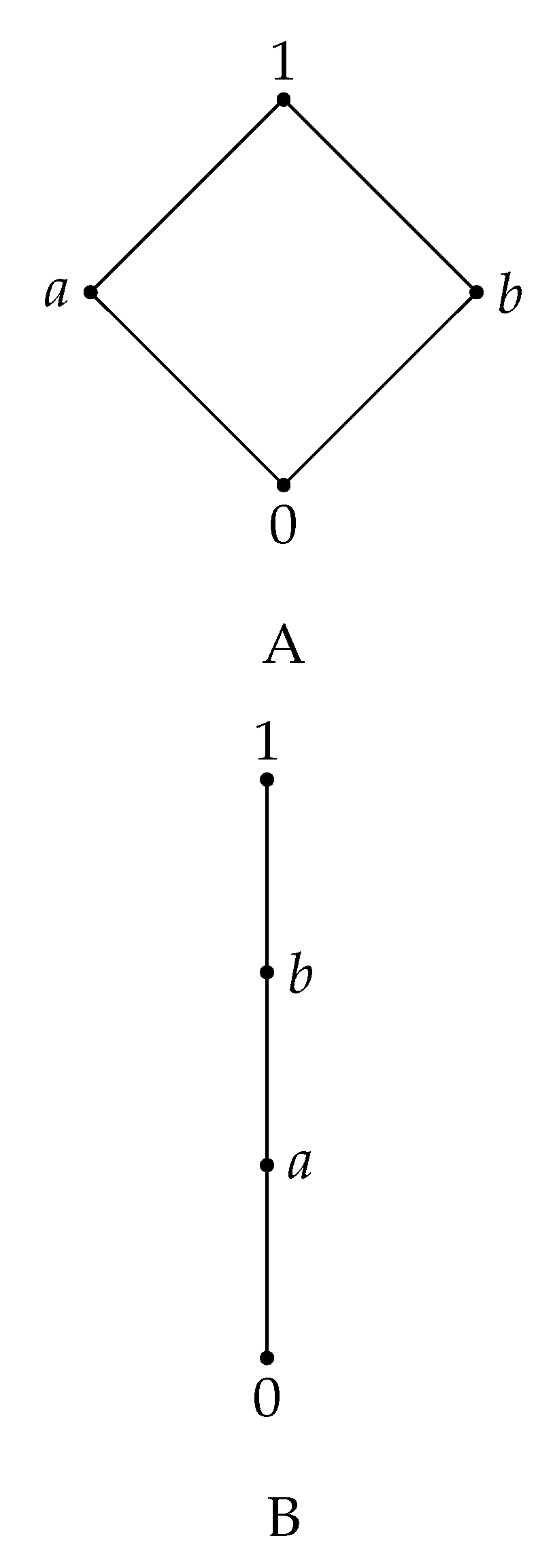
Remark 10. Let L be a residuated lattice with 4 elements, . Then, the lattice L can be of the form A or B from Figure 3.
In this situation, and so, We deduce that so Indeed, if a contradiction.
Analogously,
Moreover, and Indeed, and if then a contradiction.
Also, so since implies a contradiction. It is clear that . Therefore, we obtain a Boolean algebra with the following operations:
 izomorphic with Thus satisfies + properties.
Case ii. The lattice is a chain, , as in Figure 3, B.
We have the following subcases:
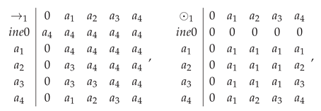
1) . We have and . Also, . Therefore, we obtain an MV-algebra structure with the following operations:
 .
.We remark that is isomorphic with and satisfies + properties.
2) . In this case we do not obtaine a residuated lattice, since ⊙ is not associative. For example, and .
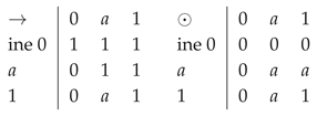
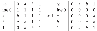
3) . We have and . Also, . Therefore, we obtain a BL-algebra structure (which is not an MV-algebra) with the following tables:
We remark that is isomorphic with and satisfies properties.
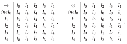
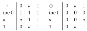
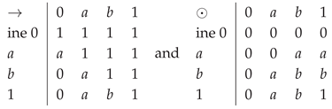
4) . We have and . Also, . Therefore, we have and , so, condition is not satisfied. It results that is not a BL-algebra, so it is only an MTL-algebra with the following tables:
 .
.We remark that is isomorphic with and satisfies property and do not satisfies property.
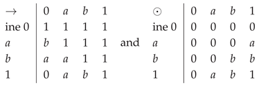
5) . We have . Also, . Therefore, we have and , false. Condition is not satisfied. It results that is not a BL-algebra. It is only an MTL-algebra with the following tables:
 .
.We remark that is isomorphic with the residuated lattice see [I; 09], p. 221, and satisfies property and do not satisfies property.
6) , it is not possible, since .
7) . We have . Also, . Therefore, for we obtain a BL-algebra structure (which is not an MV-algebra), isomorphic with with the following tables:
 .
.We remark that satisfies and properties.
8) is not possible, since .
9) . We have and . Therefore, for we obtain a BL-algebra structure (which is not an MV-algebra) with the following tables:
 .
.We remark that is isomorphic with and satisfies properties.
10) is not possible, since .
11) is not possible, since .
10) , is not possible, since from we obtain , a contradiction.
Counting the BL-algebras, MTL-algebras and divisible residuated lattices of order 4 we obtain the following result:
Proposition 11.There are 7 residuated lattices of order 4: 2 MV-algebeas 5 BL-algebras, 5 divisible residuated lattices and 7 MTL algebras.
Theorem 12.i) All residuated lattices with elements are MTL-algebras.
ii) There are no divisible residuated lattices with elements that are not MTL-algebras.
In Table 1, we briefly describe the structure of finite residuated lattices L with elements:

| Nr of residuated lattices | Structure | |
|---|---|---|
| 1 | ||
| 2 | ||
| 7 |
Table 2present a summary for the number of all residuated lattices, Boolean algebras, MV-algebras, BL-algebras, MTL-algebras and divisible residuated lattices with elements.
| All res. latt. | 1 | 2 | 7 |
| Boole | 1 | - | 1 |
| MV | 1 | 1 | 2 |
| BL | 1 | 2 | 5 |
| DIV | 1 | 2 | 5 |
| MTL | 1 | 2 | 7 |
4. The Basic Algorithm and the Made Improvements
In this section, we present a constructive algorithm for generating all residuated lattices and all made improvements which allow us to extend it to higer sizes. The initial algorithm exhaustively traverses the execution space of possible structures, verifying the axioms given in the definition of residuated lattices. Since, in this case, the execution time is very high, we improved this algorithm and we present a set of algorithmic optimizations that significantly reduce the execution space and execution time. At the end, we present other possible optimizations to achieve higher orders for n, where n is the size of a residuated lattice.
The initial algorithm exhaustively traverses the search space of possible structures, verifying the basic axioms of the residuated networks and the mentioned properties. Next, we present a set of algorithmic optimizations that significantly reduce the search space and execution time. Finally, we present other possible optimizations to achieve higher orders of n: (1) canonicalization of the order relation to avoid repeated generation of isomorphic structures, (2) intelligent pruning of backtracking for the ⊗ operation based on lower/upper bounds and local checks (partial monotonicity and right distributivity), and (3) efficient isomorphic deduplication using the network automorphism group. We discuss the benefits of each optimization and current limitations, as well as possible directions for further improvement.
5. Basic Algorithm
The constructive algorithm systematically explores all candidate structures, going through the following essential steps:
1. Generation of posets (partially ordered sets) with 0 and 1fixed. First, all possible order relations (posets) on the set that have 0 as the minimum element and 1 as the maximum element are generated. The representation of the relation ≤ is done by its transitively closed adjacency matrix (a Boolean matrix ). Specifically, we examine each subset of comparable pairs with as possible edges in the graph, compute the transitive closure (using the Roy–Warshall algorithm), and then filter out the results that are not antisymmetric (i.e., remove graphs containing cycles and with ). The algorithm ensures that 0 remains the smallest element (i.e., for any x) and 1 the largest ( for any x). The code snippet below illustrates the generation of all posets labeled with 0 minimum and 1 maximum, using the Floyd–Warshall algorithm for transitivity:
\{Floyd--Warshall on Boolean relations and the generation of posets labeled
with \$0\$ minimum and \$1\$ maximum.\}
def floyd(tc: List[List[bool]]) -\TEXTsymbol{>} None:
n = len(tc)
for k in range(n):
for i in range(n):
if tc[i][k]:
for j in range(n):
if tc[k][j]:
tc[i][j] = True
def generate\_posets(n: int):
pairs = [(i, j) for i in range(n) for j in range(i + 1, n)]
for mask in range(1 \TEXTsymbol{<}\TEXTsymbol{<} len(pairs)):
\# initialize the adjacency matrix for the identity relation (\TEXTsymbol{<}%
= reflexive)
tc = [[False] * n for \_ in range(n)]
for i in range(n):
tc[i][i] = True
\# apply subset of pairs after bitmask
for bit, (i, j) in enumerate(pairs):
if mask \& (1 \TEXTsymbol{<}\TEXTsymbol{<} bit):
tc[i][j] = True
floyd(tc) \# transitive closure
\# check antisymmetry
if any(i \TEXTsymbol{<} j and tc[i][j] and tc[j][i] for i in range(n) for j
in range(i+1, n)):
continue
\# force 0 bottom and 1 top
if not all(tc[0][x] for x in range(n)) or not all(tc[x][n-1] for x in
range(n)):
continue
yield tc
The result of this step is the set of all possible posets on n elements (labeled) with 0 minimum and 1 maximum. The complexity increases rapidly with n, because the number of labeled posets is very large (roughly, there are possible binary relations, although most will be eliminated by the antisymmetry conditions and 0, 1 extremes).
2. Lattice test and determination of ∧ and ∨ operations. For each generated poset, it is checked whether it forms a lattice with 0 and 1. The lattice condition assumes the existence of an infimum (∧, meet) and a supremum (∨, join) for any pair of elements in L. Basically, for each two elements , the set () and the set () are calculated. If either of these two sets does not have a unique minimum (respectively maximum) element, the structure is not a network and is rejected. Otherwise, the element (the maximum of the first set) and (the minimum of the second set) are determined, building the tables of the binary operations ∧ and ∨ on L. The following pseudocode extracts the ∧ and ∨ operations by traversing all pairs of elements:
def compute\_lattice(tc: List[List[bool]]):
n = len(tc)
meet = [[-1]*n for \_ in range(n)]
join = [[-1]*n for \_ in range(n)]
for a in range(n):
for b in range(a, n): \# we only consider a \TEXTsymbol{<}= b to avoid
duplication of pairs
\# the set of elements \TEXTsymbol{>}= a and \TEXTsymbol{>}= b (candidates
for a v b)
upper = \{c for c in range(n) if tc[a][c] and tc[b][c]\}
\# the set of elements \TEXTsymbol{<}= a and \TEXTsymbol{<}= b (candidates
for a \symbol{94}b)
lower = \{c for c in range(n) if tc[c][a] and tc[c][b]\}
lub = \{c for c in upper if not any(tc[c][d] and c != d for d in upper)\} \#
minimums in upper
glb = \{d for d in lower if not any(tc[d][c] and d != c for c in lower)\} \#
maximums in lower
if len(lub) != 1 or len(glb) != 1:
return None \# not a network (lub or glb is not unique)
j = lub.pop(); m = glb.pop()
join[a][b] = join[b][a] = j
meet[a][b] = meet[b][a] = m
return meet, join
If the above function returns None it means that the poset was not a valid network and is ignored. For accepted posets, we retain the ∧ and ∨ tables for the next steps.
3. Enumeration of the ⊗ operation table (commutative monoid). Having fixed the lattice structure () for a valid poset, the next step is to generate all possible ⊗ operations (multiplications) that can complete the structure into a commutative monoid with the unit 1 (neutral element) and absorbing element 0. In addition, since we work with residual algebras (MTL/BL logics), we also impose the natural constraint (the multiplication is at most as small as ∧, element by element). The algorithm backtracks through all possible completions of the ⊗ table, cell by cell, respecting the following conditions during generation:
- Initial conditions: 0 is absorbing ( for any x) and 1 is neutral (). These values are pre-filled in the ⊗ table before backtracking.
- Commutativity: The table is symmetric (), so the algorithm only goes through half of the table cells (where for the row vs. column index).
- Constraint : For any , the value assigned to cannot exceed (in the sense of the ≤ order of the lattice) . In numerical terms (given that the elements are in the ≤ order), this means ; so if (from the previously computed meet table), then must be chosen from the set .
We recursively explore each empty cell of the ⊗ table, assigning it in turn an admissible value (respecting commutativity and ) and rejecting (backtrack) if any condition is violated. Finally, when all cells are filled, the associativity of ⊗ is checked on the entire table (the condition for all ). Only associative tables are kept as valid solutions. Below is a code fragment illustrating the basic ⊗ table generation scheme (without additional optimizations):
def associative(tbl: List[List[int]]) -\TEXTsymbol{>} bool:
n = len(tbl)
return all(tbl[tbl[a][b]][c] == tbl[a][tbl[b][c]]
for a in range(n) for b in range(n) for c in range(n))
def gen\_monoid(meet: List[List[int]],tc:List[List[bool]], n: int):
top = n - 1
\# initialize the * table with -1 (unknown) and set the initial conditions
base = [[-1] * n for \_ in range(n)]
for i in range(n):
base[i][0] = base[0][i] = 0 \# 0 * i = 0
base[i][top] = base[top][i] = i \# 1 * i = i
cells = [(i, j) for i in range(n) for j in range(i, n) if base[i][j] == -1]
def backtrack(k: int):
if k == len(cells): \# basis of recursion: full table
tbl = [[base[i][j] if base[i][j] != -1 else base[j][i]
for j in range(n)] for i in range(n)]
if associative(tbl):
yield tbl \# produces a valid solution
return
i, j = cells[k]
\# iterate through possible values 0..meet[i][j]
m = meet[i][j]
candidates = [d for d in range(n) if tc[d][m]]
for val in candidates:
base[i][j] = base[j][i] = val
yield from backtrack(k + 1)
base[i][j] = base[j][i] = -1 \# backtrack: reset
yield from backtrack(0)
In the above code, meet is the computed table of ∧ (which gives the upper bound for ⊗), and the list cells contains the coordinates in the upper triangle of the table (including the diagonal) that need to be filled. At the time of initial generation (without optimizations), backtracking tries all possible values between the default lower bound 0 and the upper bound meet[i][j] for each cell, which leads to a combinatorial explosion as n increases. The complexity of this step is, in the worst case, exponential in the number of unassigned cells (approximately after setting the initial conditions). However, for small n (e.g. ), this generation is feasible and produces all candidate tableaux ⊗ compatible with the given network.
4. Calculating residuated → and checking the adjunction property. For each generated structure , we compute the implication operation → as the residue of ⊗. Specifically, for any two elements , we define:
where the order ≤ is that of the network (determined by the poset). The intuition is that is the largest element d that, multiplied by a, gives a result . If this maximum is not unique (or does not exist), then the current structure does not satisfy the axiom and is rejected. After computing the tableau of →, the adjunction is checked: for all we must have if and only if . If there is any triple that violates this equivalence, the structure is invalidated. In practice, once ⊗ is associative and → is defined as above, the adjunction property is guaranteed by construction, but the implementation explicitly checks this as a safety measure.
5. Classifying the result and eliminating isomorphic doubles. At this point, if a structure has passed all the axiomatic tests, it is classified based on the prelinearity and divisibility properties. This is done by checking the definition conditions mentioned above: if is true in the structure, then prelinearity is satisfied; similarly for divisibility . Based on these two properties, each generated model is labeled as pure MTL (prel=true, div=false), pure DIV (div=true, prel=false) or BL (prel=true, div=true).
Finally, to avoid redundant enumerations, an isomorphic deduplication is applied: many generated structures can be equivalent under element renaming (algebra isomorphism). Initially, the algorithm treats all elements in L as distinctly labeled, so the same algebras can appear several times under different permutations of the labels . To filter out isomorphic duplicates, we proceed as follows: we consider all permutations of the set that fix elements 0 and 1 (since we conventionally choose to represent each isomorphic class by having 0 and 1 in their standard roles). For each such permutation, is applied to the structure labels (on all of them: on the order relation, on the implication and on the operation tables) and the result is serialized (for example, one can concatenate the elements of the matrix of ⊗ and the upper triangle of the matrix ≤ together with the matrix of → into a string). The canonical representative of the isomorphism class is chosen as the minimal lexicographical string obtained from all possible permutations. The algorithm stores only the structures whose serialized string is minimal – eliminating those that do not correspond to the canonical representative (they are duplicates). This method ensures that each isomorphic algebra class is reported only once.
In the initial implementation, isomorphic deduplication has a significant cost, since the number of permutations to check is (all permutations of interior elements, except 0 and 1). For n up to 6 or 7 this is feasible, but quickly becomes impractical for larger n.
Basic complexity summary: The search space of the basic algorithm is dominated by the number of labeled posets (step 1) and the degrees of freedom in filling the ⊗ table (step 3). Even with the constraint , the number of possible monoidal tableaus remains huge, causing the running time to grow exponentially with n. In practical terms, the first version of the code was able to generate the complete algebras up to order in reasonable time, but at the running time exploded exponentially, exceeding acceptable limits. This observation motivated the development of targeted optimizations, described in the following section.
6. Currently Implemented Optimizations
To extend the exploration to higher-order algebras and reduce the computational time, several optimizations have been added to the algorithm. Below we present each such optimization, explaining the changes made compared to the initial version and the practical effect (reduction of execution time by pruning of the search space).
7. Optimized Filling Order of the ⊗ Table
In the initial version, the cells of the ⊗ operation table were filled in an implicit order (i.e., by traversing the rows and columns in lexicographic sequence). The current version modifies this strategy by sorting the list of unfilled cells in increasing order of the values of the infimum (∧) for each pair of elements. In other words, the cells are filled according to the constraint , so that pairs with smaller (and therefore potentially more restrictive as admissible values) are explored first. Compared to the old version, which treated the cells in a fixed order, this sorting causes conflicts to appear earlier in the backtracking process, eliminating impossible branches at a lower depth of the search tree. Basically, by filling the positions with fewer possible options first, early pruning is achieved and the exploration is considerably accelerated.
8. Incremental Associativity Checks
The current implementation also performs partial associativity checksduring the construction of the ⊗ table. More precisely, after each new assignment , the algorithm tests whether this value immediately produces a violation of the associative relation for a triplet of elements in L whose partial products have already been established. The check is incremental: only the cases "visible" in the current state of the table are considered (situations in which expressions of the form and can be completely evaluated based on the already known values). If any such situation is identified in which the associativity equality is violated by the current value v, then the respective completion cannot lead to a final associative table and the branch is immediately abandoned.
9. Differences and Practical Impact
In the original version, the associativity of ⊗ was checked only at the end, after the entire table was complete. This meant that many branches were explored in full, although they may have contained a latent associative inconsistency from the middle. The new version, by partially checking associativity, manages to detect some of these incompatibilities much earlier. Although the associativity test is expensive in general, its local form applied at each step is feasible and brings pruning benefits: it reduces the number of unnecessary additions and contributes to the overall efficiency of backtracking.
10. Representing Posets with Bitmasks
Each element of the poset and its successors can be encoded as a bitmask, where the bit k indicates whether the current element is ≤ to the element k. This representation transforms set operations (e.g. union or intersection of successors) into very fast bitwise operations: intersection becomes a logical AND, union becomes a logical OR, etc. Thus, transitive closure or composition calculations are reduced to bitwise operations, significantly speeding up the algorithm.
11. Incremental Propagation of Transitive Relations
In the incremental construction of the poset, each time a new comparability relation is added, the transitive closure is immediately updated. Basically, when j becomes a successor of i, we update the bit mask of i with the OR of the mask of j, thus capturing all its transitive descendants. This operation is equivalent to one step in the Warshall algorithm (update with OR/AND), but is done incrementally, thus avoiding complete recalculations of the closure.
12. Optimizing the Residuation Calculation with Bit Mask
The internal residuation (the implication in the poset) is calculated by finding the maximal element x such that . Using the bit representation, the candidate set is filtered by bitwise operations: we intersect the bit masks of the possible successors of a with the condition . Since bitwise operations are very fast (significantly faster than complex arithmetic operations), this procedure considerably speeds up the residue determination.
By combining the above optimizations (cell sorting, associativity checks during generation, use of bitwise operations), the current version of the algorithm manages to explore the space of possibilities much more efficiently. Experimentally, these improvements extended the threshold of complete enumeration up to (all algebras of order 7 could be generated at a reasonable cost), which was not feasible in the original version (which basically stopped at before becoming unaffordable). However, for , the search space remains prohibitive even with the implemented optimizations, which motivates the development of additional strategies, described in the next section.
13. Planned Future Optimizations
Although the current optimizations have pushed the model enumeration frontier up to , there are still significant limitations that prevent the algorithm from scaling to larger n. The main obstacles are: (a) the fact that the generation of networks (posets) is still performed at the level of labeled structures (even if many duplicates are subsequently filtered out, the complexity of poset enumeration increases greatly for large n), and (b) the cost of isomorphism checking based on generating all permutations increases exponentially with increasing n.
To overcome these limitations and extend the exploration to higher orders ( and above), several optimizations and additional approaches are planned, as follows.
14. Canonization at the Level of the Order Relation (Poset)
Instead of the algorithm enumerating and testing all labeled posets (step 1) to discover the isomorphically distinct ones, we plan to apply a canonization of the poset itself during generation. The idea is to define a canonical criterion (e.g., lexicographic) for representing the transitivity matrix of the relation ≤ under the action of permutations of the set L (fixing the elements 0 and 1). Thus, when generating the posets, we will be able to skip those that are isomorphic to already generated ones, keeping only the canonical representative of each order isomorphism class.
The planned concrete implementation would group the intermediate elements into equivalence classes based on simple invariants (such as the number of elements above and below in the poset, i.e. the values and for each element x). Then, by backtracking, only permutations that respect these groupings would be explored (i.e. only elements with the same are permuted among themselves). For each generated poset, the minimal representative string (serialization of the upper triangle of the adjacency matrix ≤) will be determined and used as the canonical identifier. If a newly generated poset has the same identifier as one already seen, it will be ignored.
Expected benefit: Such canonicalization would eliminate duplicate isomorphic networks from the very beginning, dramatically reducing the number of posets on which we have to run the subsequent steps (completion of ⊗ etc.). Basically, the effort of exploring posets would decrease from enumerating all labeled ones (which contain redundancy of order in the worst case) to enumerating only the non-isomorphic ones. For example, for , this optimization would bring a substantial gain, since the number of distinct networks is much smaller than the number of raw labeled networks.
15. Dynamic Lower Bounds and Local Prunes in Backtracking for ⊗
The most difficult step remains the filling of the table for the ⊗ operation. To make backtracking more efficient and avoid exploring obviously impossible configurations, two types of optimizations will be added to the generation of ⊗:
- Calculating a dynamic lower bound: In addition to the already used upper bound (i.e. ), we will also introduce a lower bound dynamically calculated for each cell being filled. Intuitively, represents the smallest value that would be constrained to take, given the values already established in the table. It will be calculated as follows:
i.e. the join of all known products where and . This set includes, in particular, the cases or if these products have already been filled in. The lower bound will be calculated incrementally as the table is filled in, using the current values in the table and the table of ∨. Anticipated impact: Instead of backtracking the value from 0 to , we will be able to start directly from , considerably reducing the number of candidate values tried for that cell.
- Local consistency checks (prunes): After assigning a provisional value to a cell , two local tests will be applied immediately to detect violations of the monotonicity and right distributivity properties:
- Partial monotonicity: If in the poset, then for any known z we must have and . During the completion of the table, not all values are determined, but if both and (or symmetrically and ) have already been determined, we will immediately check that the order relationship between the results corresponds to that between the operands. Any inversion (i.e. we find , but the value assigned to is not ≤ than ) indicates a violation of monotonicity, and the branch will be pruned (pruned) on the spot.
- Right distributivity (local):
The right distributivity axiom in residual networks states that for any . During partial generation, we will not be able to verify this formula completely for all (many values are missing), but we will identify local cases where both , , and have been established. If in such restricted situations the relation is violated by the current assignment, then we will know for sure that the full extension will not satisfy the right distributivity, so the branch can be stopped early.
It is anticipated that, with these improvements, the backtracking procedure for monoids will become much more efficient. The code snippet below shows a possible pseudocode for an optimized generation of ⊗, integrating the calculation of bounds and local prunes into the recursive loop:
def lower\_bound\_for\_cell(base, i, j, tc, join) -\TEXTsymbol{>} int:
"""Calculate lb(i,j) based on the values already established in the base
table."""
n = len(base); current\_lb = None
for c in range(n):
if not tc[c][i]: \# c \TEXTsymbol{<}= i ?
continue
for d in range(n):
if not tc[d][j]: \# d \TEXTsymbol{<}= j ?
continue
v = base[c][d]
if v \TEXTsymbol{<} 0:
continue \# if c*d is not yet set, skip it
current\_lb = v if current\_lb is None else join[current\_lb][v]
return current\_lb if current\_lb is not None else 0
def partial\_monotone\_ok(base, tc, i, j) -\TEXTsymbol{>} bool:
"""Check partial monotonicity on known rows/columns i,j."""
n = len(base); vij = base[i][j]
for d in range(n):
vd = base[i][d] \# i * d
if vd \TEXTsymbol{>}= 0: \# if i*d is known
\# i \TEXTsymbol{<}= j =\TEXTsymbol{>} (i*d) \TEXTsymbol{<}= (j*d) ?
if tc[j][d] and not tc[vd][vij]:
return False
\# j \TEXTsymbol{<}= d =\TEXTsymbol{>} (i*d) \TEXTsymbol{>}= (j*d) ?
if tc[d][j] and not tc[vij][vd]:
return False
for c in range(n):
vc = base[c][j] \# c * j
if vc \TEXTsymbol{>}= 0:
\# c \TEXTsymbol{<}= i =\TEXTsymbol{>} (c*j) \TEXTsymbol{<}= (c*i) ?
if tc[i][c] and not tc[vc][vij]:
return False
\# i \TEXTsymbol{<}= c =\TEXTsymbol{>} (c*j) \TEXTsymbol{>}= (c*i) ?
if tc[c][i] and not tc[vij][vc]:
return False
return True
def partial\_rdist\_ok(base, join, i, j) -\TEXTsymbol{>} bool:
"""Check the local right distributivity for row i and column j."""
n = len(base)
for b in range(n):
for c in range(n):
if join[b][c] == j: \# if (b V c) = j in lattice
ab = base[i][b] \# a*b (a = i)
ac = base[i][c] \# a*c
if ab \TEXTsymbol{>}= 0 and ac \TEXTsymbol{>}= 0:
\# compare a*(b V c) with (a*b) V (a*c)
if base[i][j] != join[ab][ac]:
return False
return True
def gen\_monoid\_with\_bounds(meet, join, tc, n):
top = n-1
base = [[-1]*n for \_ in range(n)]
\# initializations 0 absorbent and 1 neutral as before
for i in range(n):
base[i][0] = base[0][i] = 0
base[i][top] = base[top][i] = i
cells = [(i, j) for i in range(n) for j in range(i, n) if base[i][j] == -1]
\# sort the cells so that the most restrictive ones (with smaller meet) are
filled first
cells.sort(key=lambda ij: meet[ij[0]][ij[1]])
def backtrack(k: int):
if k == len(cells):
\# complete table, will check associativity at the end
tbl = [[base[i][j] if base[i][j] != -1 else base[j][i]
for j in range(n)] for i in range(n)]
if associative(tbl):
yield tbl
return
i, j = cells[k]
\# dynamically calculate the bounds for this cell
lb = lower\_bound\_for\_cell(base, i, j, tc, join)
ub = meet[i][j]
candidates = [d for d in range(n) if tc[d][ub] and tc[lb][d]]
for val in candidates:
base[i][j] = base[j][i] = val
\# apply local prunes before recursively descending
if partial\_monotone\_ok(base, tc, i, j) and partial\_rdist\_ok(base, join,
i, j):
yield from backtrack(k + 1)
base[i][j] = base[j][i] = -1 \# return (backtrack)
yield from backtrack(0)
In the above pseudocode, the function gen_monoid_with_bounds represents the planned optimized version of the monoid generator. The main observations about this approach would be:
- The list of cells to be filled will be sorted in ascending order of ∧ values (cells with small meet, hence potentially more restrictive, will be approached first to cause early prunes).
- For each cell , the values tried would be from the new lower bound lb (computed based on the values already set) up to ub = meet[i][j]. Thus, a lot of unnecessary lower values would be automatically skipped that would have been implicitly eliminated by the order constraints anyway.
- After setting a candidate value
val in the cell, partial_monotone_ok and partial_rdist_ok will be checked immediately. These functions test local monotonicity and distributivity conditions based on the values already known in the table (note that they only use base[...] entries that have been filled in, the unfilled ones being and not influencing the checks). If any test fails, the branch will be cut without continuing deeper.
- Full associativity will still be checked only at the end, at the backtracking leaf (it is more efficient to leave the full global associativity check at the end, although theoretically it could also be tested incrementally in part).
Expected benefits of these optimizations: The introduction of dynamic bounds and local prunes would drastically reduce the number of explored ⊗ table configurations. Branches that would lead to monotonicity or distributivity violations would be eliminated very early, and the ranges of possible values for each cell would be significantly narrowed. Based on the performances observed in current optimizations, we estimate that this optimized version of backtracking could lead to a jump from the impossibility of completing the case (with the original algorithm) to obtaining the full result for in reasonable time. However, for , even with these improvements, the search space would still be too large, which will probably require further optimizations or a change in strategy (see the discussion below for other directions).
16. Isomorphic Deduplication Based on the Network Automorphism Group
The last major planned optimization aims to reduce the cost of isomorphic deduplication (the final step of the algorithm). Instead of testing all permutations for each structure (to determine the canonical representative of the isomorphism class), we plan to explicitly compute the automorphism group of the current network and use only this group (a much smaller set of permutations) to identify the isomorphism classes of the ⊗ tables.
An automorphism of the network is a permutation of the set L that preserves the order relation (i.e. ). The automorphisms form a group (under composition), and the size of this group depends on the internal symmetries of the poset. For example, if the network is a completely ordered chain, then will be practically trivial (just the identity), while if the network has non-trivial symmetries (e.g. two incomparable interchangeable elements), the group will contain more non-trivial permutations.
The optimized algorithm would determine by a backtracking similar to poset canonization: we will group equivalent elements (according to invariants of degree, level, etc. in the poset) and try permutations of these elements, checking the invariance of the relation ≤. This will obtain the list of all poset automorphisms. Then, for a given structure (a certain completion ⊗ on the respective poset), the canonical representative of the isomorphism class can be computed without exploring all possible permutations, but by applying only each automorphism to the table of ⊗ and choosing the encoding (serialized string) that is lexicographically smallest. Intuitively, we will restrict ourselves to the relevant permutations (poset symmetries); permutations that are not automorphisms of the network will not produce structurally distinct algebras, since they move elements between positions that are not structurally equivalent.
Estimated benefit: This improvement would drastically reduce the complexity factor of deduplication. Instead of permutations (which for means cases, and for would be and so on), only permutations would be analyzed. Usually, is much smaller than the factorial, especially for "asymmetric" posets. In ideal cases, the poset has very few automorphisms (only the identity), so practically no additional comparison is needed; even in cases with non-trivial symmetries, there would be enormous savings compared to the naive approach. With this optimization, we expect that the memory and time consumption for isomorphism filtering would decrease considerably, especially at the upper bounds of the explored n.
In addition to the major optimizations described above, we explore other possible directions for improving the algorithm, such as:
- Direct generation ofnon-isomorphicposets: Instead of enumerating all labeled posets and canonizing them later, one can adopt a canonical augmentation strategy (used for example in graph or non-isomorphic poset generation algorithms). This would build the networks gradually, adding one element at a time and imposing canonical conditions at each step, so that each non-isomorphic network is generated only once. Such a method would completely eliminate isomorphic redundancy already in the poset generation phase, saving enormously for large n.
- Using a dedicated solver for automorphisms: Automorphism finding problems can be approached much more efficiently with graph theory tools,
such as nauty-type algorithms or other specialized solvers. By transforming the network (or network with operations) into a graph and using such tools, we could quickly compute the automorphism group even for larger structures, avoiding the manual backtracking implemented in Python.
- Other heuristic optimizations and parallel execution: For example, implementing additional symmetry breaking in the generation of ⊗ (such as conditions that fix certain order relations between the rows in the ⊗ table to avoid equivalent permutations) or running the algorithm in parallel (distributing the input posets between multiple computational processes) could bring significant performance gains. Also, any additional theoretical knowledge about these algebras (new logical constraints, structural theorems) could be used to reduce the search space.
In conclusion, the presented algorithm, together with the current optimizations, represents an efficient compromise between generality and efficiency in the problem of generating finite residual algebras. It allowed the complete exploration of the model space for small sizes and provides a platform from which it can be extended to even higher orders by developing the optimization ideas discussed above.
In the specialized literature, such algebras up to are known, through an alternative algorithm. By the present different approach, we succeeded in generating algebras up to order . By the proposed optimizations we believe that the order can be exceeded and high orders can be reached.
Regarding the number of algebras in each analyzed family, we obtained the following results after the programs have been run (see the following table):
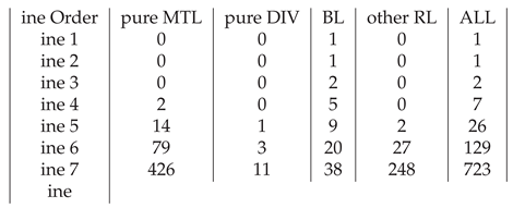
By ,,pure MTL” we understand MTL-algebras which are not BL-algebras and by ,,pure DIV” we understand DIV algebras which are not BL-algebras, by ,,other RL” we understand residuated lattices which are not MTL, DIV or BL and by ,,ALL”, we understand all residuated lattices.
Conclusions. In this paper we present some properties of divisible residuated lattices and MTL-algebras. These structures have a important significance in the study of fuzzy logic. From computational considerations, we analyzed the structure of these residuated lattices of small size n () and we gave summarizing statistics. These results can be extended for higer size, by using computer and a constructive algorithm for generating all residuated lattices.
References
- [BV; 10], Belohlavek, R., Vychodil, V., Residuated Lattices of size Order, 27(2010), 147-161.
- [Bl; 53] Blair, R.L, Ideal lattices and the structure of rings, Trans. Am. Math. Soc., 75(1953), 136–153.
- [BP; 02] Busneag, D., Piciu, D., Lectii de algebra, Ed. Universitaria, Craiova, 2002.
- [CFP; 23] Călin, M. F., Flaut, C., Piciu, D., Remarks regarding some Algebras of Logic, Journal of Intelligent & Fuzzy Systems, 45(5)(2023), Journal of Intelligent & Fuzzy Systems, 45(5)(2023), 8613-8622, DOI: 10.3233/JIFS-232815.
- [COM; 00] Cignoli, R.; D’Ottaviano, I.M.L.; Mundici, D., Algebraic Foundations of many-valued Reasoning. Trends in Logic-Studia Logica Library 7, Dordrecht: Kluwer Acad. Publ.2000.
- [CHA; 58] Chang, C.C.,Algebraic analysis of many-valued logic, Trans. Amer. Math. Soc. 88(1958), 467-490.
- [NL; 03] Di Nola, A., Lettieri, A., Finite BL-algebras, Discrete Mathematics, 269 (2003), 93—112.
- [Di; 38] Dilworth, R.P., Abstract residuation over lattices, Bull. Am. Math. Soc. 44(1938), 262–268.
- [E] Esteva, F., Godo, L., Monoidal t-norm based logic : towards a logic for left-continuous t-norms, Fuzzy Sets and Systems, 124 (2001), 271-288.
- [F] Fodor, J.K., Contrapositive symmetry of fuzzy implications, Fuzzy Sets and Systems, 69 (1995), 141-156.
- [FP; 22] Flaut, C., Piciu, D., Connections between commutative rings and some algebras of logic, Iranian Journal of Fuzzy Systems, 19 (6) (2022), 93-110.
- [FP; 23] Flaut, C., Piciu, D.,Commutative Rings Behind Divisible Residuated Lattices, Mathematics 2024, 12(23), 3867; https://doi.org/10.3390/math12233867
- [I; 09] Iorgulescu, A., Algebras of logic as BCK algebras,A.S.E., Bucharest, 2009.
- [KS; 24] Koohnavard R., Saeid A.B., Residuated skew lattices with modal operator, An. Şt. Univ. Ovidius Constanţa, 31(1),2023, 167–179, DOI: 10.2478/auom-2023-0008.
- [S] Swamy K.L.N., Dually residuated lattice ordered semigroups, Mathematische Annalen, 159 (2) (1965), 105-114.
- [TT; 22] Tchoffo Foka, S. V., Tonga, M., Rings and residuated lattices whose fuzzy ideals form a Boolean algebra, Soft Computing, 26 (2022) 535-539.
- [T; 99] Turunen, E., Mathematics Behind Fuzzy Logic, Physica-Verlag, 1999.
- [WD; 39] Ward, M., Dilworth, R.P., Residuated lattices, Trans. Am. Math. Soc. 45(1939), 335–354.
Disclaimer/Publisher’s Note: The statements, opinions and data contained in all publications are solely those of the individual author(s) and contributor(s) and not of MDPI and/or the editor(s). MDPI and/or the editor(s) disclaim responsibility for any injury to people or property resulting from any ideas, methods, instructions or products referred to in the content. |
© 2025 by the authors. Licensee MDPI, Basel, Switzerland. This article is an open access article distributed under the terms and conditions of the Creative Commons Attribution (CC BY) license (http://creativecommons.org/licenses/by/4.0/).
Copyright: This open access article is published under a Creative Commons CC BY 4.0 license, which permit the free download, distribution, and reuse, provided that the author and preprint are cited in any reuse.


