Submitted:
01 October 2025
Posted:
02 October 2025
You are already at the latest version
Abstract
Financial institutions operating distributed machine learning systems face an emerging class of stealth adversaries who exploit temporal patterns across training cycles to inject persistent backdoors that remain dormant for months before activation. Unlike conventional single-round attacks, these sophisticated temporal poisoning strategies leverage sequential dependencies to bypass existing detection mechanisms while gradually compromising model integrity. Current defense frameworks remain fundamentally inadequate against such multi-period adversarial choreography, particularly in high-stakes financial environments where minute perturbations can trigger systemic failures. Existing security frameworks largely focus on static threat models and fail to address sophisticated multi-period adversarial strategies that unfold over time in financial transaction streams. To address these challenges, we propose DEFEND, a comprehensive defense framework that integrates temporal behavior analysis, robust statistical aggregation, and multi-scale verification into a unified multi-layer architecture. Our framework formulates defense coordination as a Markov Decision Process and employs Proximal Policy Optimization for adaptive policy learning that dynamically balances security enforcement with model utility. We design three sophisticated temporal attack models to comprehensively evaluate our defense mechanism: fixed-period data poisoning, multi-period data poisoning, and model weight poisoning attacks. The multi-layer defense architecture combines geometric median-based robust aggregation with Dynamic Time Warping pattern matching and adaptive client participation control. Extensive experiments on CIFAR-10, FEMNIST, and MNIST datasets demonstrate that DEFEND achieves superior defense performance with success rates of 95.6% for ResNet-18 and 94.0% for MobileNet V2, while maintaining clean accuracy levels between 85-95% across various data heterogeneity levels and malicious client ratios. Our framework provides theoretical guarantees for Byzantine robustness and practical scalability for moderate-scale federated deployments, making it well-suited for real-world financial applications requiring both security and efficiency.
Keywords:
federated learning
; temporal backdoor attacks
; financial security
; deep reinforcement learning
; Byzantine robustness
; Markov decision process
; geometric median aggregation
; adaptive defense coordination
; multi-layer security
; temporal behavior analysis
1. Introduction
1.1. Background
The financial industry is undergoing rapid digital transformation, with institutions increasingly relying on distributed machine learning techniques to improve fraud detection, risk management, and regulatory compliance. Federated learning (FL) has emerged as a promising paradigm to enable collaborative intelligence across banks, payment platforms, and other financial entities while maintaining data privacy [1,2,3]. By allowing participants to train shared models without centralizing raw data, FL provides a natural fit for sensitive financial applications where strict privacy regulations and competitive concerns prevent data sharing.
However, the adoption of FL in financial systems introduces significant security challenges. Recent studies highlight that FL is inherently vulnerable to poisoning and backdoor attacks, where malicious participants inject crafted updates to manipulate global models [4,5]. These attacks can be particularly damaging in financial environments, where small perturbations may lead to large-scale fraud or systemic risks. Beyond traditional single-round threats, researchers have uncovered persistent backdoor strategies that exploit temporal dependencies across multiple training rounds, allowing attackers to evade conventional defenses and achieve long-term stealth [6,7]. Such temporal vulnerabilities are especially critical in financial transaction streams, which naturally exhibit sequential correlations and evolving patterns.
To address these challenges, researchers have proposed robust aggregation methods and privacy-enhancing techniques to mitigate adversarial updates in FL. Approaches such as robust learning rate adjustment [8,9,10] and privacy-preserving backdoor defenses for heterogeneous data distributions [11] have demonstrated effectiveness under certain threat models. Nevertheless, most of these methods remain static and fail to capture multi-period adversarial strategies that unfold over time. Moreover, existing solutions often trade accuracy for security, limiting their practicality in high-stakes domains like finance where both precision and reliability are paramount.
Meanwhile, reinforcement learning (RL) has shown considerable potential for adaptive cybersecurity, offering dynamic decision-making in the face of evolving adversarial behaviors [12]. By framing defense coordination as a sequential decision problem, RL methods can enable financial FL systems to respond adaptively to temporal threats, balancing security enforcement with model utility. This motivates the development of integrated frameworks that combine multi-layered defenses with RL-based coordination to address sophisticated temporal backdoor attacks in financial federated learning environments.
1.2. Motivation and Contributions
Despite growing efforts to enhance the robustness of federated learning, several critical research gaps remain unaddressed in the context of financial systems:
- 1.
- Existing security frameworks do not adequately account for temporal backdoor attacks that exploit sequential dependencies in financial transaction streams. Most defenses assume static or isolated threat models, overlooking coordinated multi-round adversarial strategies.
- 2.
- Current defense mechanisms are largely single-layered and static, focusing either on aggregation robustness or anomaly detection, without integrating multiple complementary layers that can collectively enhance resilience against adaptive attackers.
- 3.
- Few approaches incorporate dynamic coordination mechanisms to balance security and utility. Static thresholds or fixed strategies cannot adapt to changing adversarial intensity, heterogeneous client behaviors, and evolving network conditions.
To address these gaps, this work introduces DEFEND, a comprehensive defense framework for federated learning in financial systems. Our framework integrates temporal behavior analysis, robust statistical aggregation, and multi-scale verification into a multi-layered architecture, while employing a Markov Decision Process (MDP) formulation and reinforcement learning for adaptive coordination. The contributions of this paper are summarized as follows:
- We formalize temporal backdoor threats in federated financial learning by characterizing attack strategies that exploit multi-period dependencies across training rounds.
- We design a multi-layer defense architecture that combines temporal behavior profiling, robust aggregation, and multi-scale verification to jointly enhance detection accuracy and resilience.
- We formulate defense coordination as an MDP problem and develop an RL-based policy using Proximal Policy Optimization (PPO) to dynamically manage defense actions, balancing robustness and model performance.
- We validate DEFEND on multiple benchmark datasets (CIFAR-10, FEMNIST, MNIST) under varying degrees of heterogeneity and adversarial participation, demonstrating superior defense success rates and detection efficiency compared to state-of-the-art baselines.
The remainder of this paper is organized as follows. Section 2 reviews existing research on federated learning security, temporal attack detection, and multi-layer defense coordination. Section 3 describes the proposed DEFEND framework. Section 4 presents experimental evaluations. Section 6 concludes and outlines directions for future work.
2. Related Work
2.1. Federated Learning Security in Financial Systems
Federated learning security in financial systems has emerged as a critical research area addressing the inherent privacy and security challenges in distributed financial data processing environments [13,14,15,16,17,18,19,20,21]. Chen et al. [13] conducted an extensive survey identifying the intricate security challenges within federated learning frameworks, emphasizing vulnerabilities in communication links and potential cyber threats across decentralized networks. Their comprehensive analysis delves into various defensive strategies and explores applications across different sectors, contributing to the development of secure and efficient federated learning systems. To address specific financial fraud detection challenges, Aljunaid et al. [14] proposed an Explainable Federated Learning (XFL) model that integrates Shapley Additive Explanations (SHAP) and LIME techniques for enhanced interpretability while maintaining privacy compliance. Their approach achieved 99.95% accuracy with a miss rate of 0.05%, effectively eliminating false positives in financial fraud classification while preserving data privacy and regulatory compliance.
Building on decentralized security considerations, Hallaji et al. [15] performed a thorough security analysis of decentralized federated learning systems, studying possible variations of threats and adversaries while overviewing potential defense mechanisms. Their work addresses server-related threats elimination through blockchain technologies, though acknowledging new privacy challenges introduced by decentralized architectures. To enhance privacy preservation in financial technology applications, Xiong et al. [20] developed a Heterogeneous Privacy-Preserving Blockchain-Enabled Federated Learning (HPP-BEFL) system specifically designed for social fintech environments. Their novel PKI and identity-based heterogeneous authenticated asymmetric group key agreement (PKI-IB-HAAGKA) protocol effectively mitigates man-in-the-middle and inference attacks while addressing crypto system heterogeneity issues.
Recent advances have also explored credit risk assessment architectures [16], behavioral anomaly detection in dynamic transaction graphs [17], and blockchain-based knowledge enhancement mechanisms [22]. However, existing federated learning security frameworks lack comprehensive temporal attack detection mechanisms and fail to adequately address sophisticated backdoor attacks that exploit temporal patterns in financial data streams, which are essential for defending against coordinated multi-period adversarial strategies in distributed financial learning environments.

Table 1.
Comparison of our work with related studies.
| Ref | [13] | [23] | [15] | [20] | [24] | [25] | [26] | [27] | [14] | [28] | [29] | Proposed work | |
| Feature | |||||||||||||
| Financial application domain | ✓ | ✓ | ✓ | ||||||||||
| Federated learning framework | ✓ | ✓ | ✓ | ✓ | ✓ | ✓ | ✓ | ✓ | |||||
| Temporal attack detection | ✓ | ✓ | ✓ | ||||||||||
| Multi-layer defense design | ✓ | ✓ | |||||||||||
| MDP/RL coordination | ✓ | ✓ | ✓ | ||||||||||
2.2. Temporal Attack Detection and Defense Mechanisms
Temporal attack detection and defense mechanisms have gained significant attention as adversaries increasingly exploit time-dependent vulnerabilities in distributed systems [24,25,30,31,32,33,34,35]. Zamanzadeh et al. [25] provided a comprehensive survey of deep learning approaches for time series anomaly detection, highlighting the importance of identifying anomalous patterns that indicate novel or unexpected events such as production faults and system defects. Their taxonomy encompasses anomaly detection strategies and deep learning models, highlighting the challenges presented by the large size and complexity of temporal patterns in time series data. Duan et al. [24] addressed practical cyber attack detection through Continuous Temporal Graph (CTG) neural networks in dynamic network systems, proposing an interaction-centered perspective that refines information interactions between network entities into CTG evolution processes. Their framework naturally incorporates new node access behaviors and presents a message aggregation scheme that fuses spatio-temporal neighborhoods with actual time distribution and historical states, demonstrating superior performance on ToN-IoT, UNSWNB15, CIC-Dark2020, and J.P. Morgan payment datasets.
To address zero-day attack challenges, Wu et al. [31] developed an active learning framework using Deep Q-Network (DQN) for intelligent sample selection with probability distribution analysis. Their approach integrates Bi-directional Long Short-Term Memory (BiLSTM) networks into the DQN model to analyze temporal correlations within static classification contexts, employing Euclidean distance functions for accurate sample labeling. Hammad et al. [33] explored deep reinforcement learning for adaptive cyber defense, implementing cutting-edge DRL techniques including Deep Q-Networks (DQN), Proximal Policy Optimization (PPO), and Twin Delayed Deep Deterministic Policy Gradient (TD3) for real-time threat discernment and neutralization across varied cyber threat scenarios ranging from malware invasions to phishing attacks and adversarial assaults.
Recent developments have also investigated spatio-temporal advanced persistent threat detection in cyber-physical power systems [30], advances in time-series anomaly detection algorithms and benchmarks [36], and security defense strategies for Internet of Things based on deep reinforcement learning [37]. However, existing temporal attack detection frameworks lack sophisticated multi-period pattern recognition capabilities and fail to address coordinated backdoor injection strategies that exploit temporal dependencies across distributed learning rounds, which are crucial for detecting and defending against sophisticated temporal poisoning attacks in federated financial learning environments.
2.3. Multi-Layer Defense and MDP-based Coordination
Multi-layer defense mechanisms and MDP-based coordination strategies have emerged as critical components for robust federated learning systems, addressing the need for comprehensive protection against sophisticated adversarial attacks [23,26,27,28,29,38,39,40,41,42]. Li et al. [28] proposed a Multi-layer Aggregation Backdoor Defense Framework (MABDF) that ensures secure model aggregation through adaptive similarity filtering, pruning mean aggregation, and subspace robust projection methods. Their three-layer architecture calculates pairwise cosine similarity between client updates with dynamic thresholds based on median and standard deviation, applies pruning mean aggregation to detect hidden gradient operations, and projects updates onto low-rank subspaces through singular value decomposition (SVD) to suppress backdoor neuron activation, achieving backdoor attack success rates below 3% while maintaining model accuracy decrease of no more than 1.5%. Uddin et al. [23] conducted a systematic literature review using the PRISMA framework, analyzing 244 studies across eight themes of robust federated learning including objective regularization, optimizer modification, differential privacy, client selection, and new aggregation algorithms, providing comprehensive insights into approaches for enhancing FL model robustness against adversarial attacks and noisy updates.
For dynamic policy coordination, Bello et al. [26] developed a security strategy incorporating zero-trust models with dynamic policy decisions through stochastic games and reinforcement learning techniques. Their approach employs Generalized Proximal Policy Optimization with sample reuse (GePPO) and its meta-learning variant GePPO-ML, along with Sample Dropout PPO with meta-learning (SDPPO-ML) for adaptive policy updates, demonstrating superior performance compared to baseline REINFORCE and PPO algorithms in next generation network security scenarios. Huang et al. [27] addressed Byzantine robustness in heterogeneous federated learning through Self-Driven Entropy Aggregation (SDEA), leveraging random public datasets to conduct robust aggregation by introducing learnable aggregation weights that minimize instance-prediction entropy while maximizing batch-prediction entropy to accommodate diverse client tendencies and detect Byzantine attackers effectively.
Recent advances have also explored multi-layered protection systems for cloud computing environments [39], safe reinforcement learning frameworks for risk-averse dispatch with frequency security constraints [40], and security metrics for assessing power grids against attacks from EV charging ecosystems using Markov decision processes [29,43]. However, existing multi-layer defense frameworks lack integrated temporal anomaly detection capabilities and fail to provide coordinated MDP-based defense mechanisms that can dynamically adapt to evolving temporal backdoor attack patterns while maintaining optimal resource allocation and system performance in distributed financial learning environments.
3. Method
This section presents our comprehensive framework for detecting and defending against temporal backdoor attacks in federated learning environments through sophisticated mathematical modeling approaches. Our methodology integrates three distinct temporal poisoning attack models, establishes a multi-objective optimization framework, employs advanced statistical analysis techniques, and formulates an MDP-based defense mechanism. The proposed system leverages deep mathematical foundations to achieve optimal detection and defense performance across diverse federated learning scenarios while maintaining computational efficiency and theoretical rigor. Method architecture is shown in the Figure 1.
3.1. Problem Formulation
Consider a federated learning system comprising N participating clients denoted as , where each client maintains local dataset over a finite communication horizon T. The temporal data sequence for client is represented as , where denotes the m-dimensional feature vector observed at communication round t. The corresponding ground truth labels are denoted as , where represents the true class label at round t from the label space .
The client operational states are characterized by a discrete state space , where represents the normal operational state, indicates a suspicious state requiring further monitoring, and denotes a confirmed poisoned state. During the poisoning process, a subset of clients with cardinality , where represents the maximum poisoning ratio, becomes compromised during specific time intervals .
Each client is characterized by a resource profile , where represents maximum computational capacity, denotes memory capacity, indicates energy budget, and specifies communication bandwidth. The available resources at round t are denoted as , where each component satisfies .
The fundamental objective of our detection framework is to minimize the overall detection error, formulated as a multi-objective optimization problem with temporal consistency constraints:
where represents the client state classification loss function, denotes the predicted client state, quantifies the temporal localization error between predicted intervals and true poisoning intervals , denotes the false positive penalty term, is the continuous cost function modeling resource consumption, represents the entropy regularization term for uncertainty quantification, and are regularization coefficients that balance different objectives.
The temporal localization error is computed using a weighted Hausdorff distance:
which ensures both precision and recall in temporal poisoning interval detection.
3.2. Temporal Backdoor Attack Models
To comprehensively evaluate our detection framework, we design three sophisticated temporal backdoor strategies that exploit different characteristics of federated learning protocols. Each attack model represents a distinct threat vector commonly encountered in real-world federated environments, incorporating realistic constraints on attack capabilities and detectability thresholds.
3.2.1. Fixed-Period Data Poisoning Attack
The fixed-period data poisoning attack systematically injects backdoor triggers into client datasets during predetermined temporal windows, eventually culminating in significant global model degradation at coordinated trigger points. This attack strategy maintains stealth by concentrating the poisoning effect within specific time intervals while preserving normal behavior patterns outside attack periods.
For malicious client at communication round t, the poisoned local dataset is constructed according to:
where denotes the fixed attack interval, and the poisoned sample set follows a sophisticated generation process incorporating temporal dynamics and spatial correlations.
The poisoned sample construction employs multi-dimensional trigger injection with harmonic modulation:
where ⊙ denotes element-wise multiplication, represents the primary attack direction vector, K is the number of harmonic components, control amplitude and phase parameters, are harmonic weight vectors, denotes the target label, and represents the selected subset for poisoning.
The time-dependent perturbation magnitude follows an accumulative schedule incorporating memory effects and stochastic variations:
where represents the base accumulation rate, is the temporal decay factor, are stochastic scaling factors following a Markov chain with transition probabilities , the Gaussian envelope ensures smooth temporal transitions with mean and variance , controls neighborhood influence, represents neighboring clients, and captures inter-client correlation effects.
3.2.2. Multi-Period Data Poisoning Attack
The multi-period data poisoning attack exploits temporal dependencies by distributing backdoor injection across multiple non-consecutive communication rounds, creating sophisticated interference patterns that evade single-period detection mechanisms while maintaining cumulative backdoor effectiveness.
The poisoned dataset construction employs period-specific trigger variations across disjoint temporal intervals where for :
where period-specific poisoned samples incorporate adaptive trigger patterns and cross-period consistency constraints.
The multi-dimensional periodic signal injection follows:
where control injection intensities for primary and secondary periodic signals and respectively.
The primary multi-dimensional periodic signal is defined as:
where and represent the numbers of sine and cosine components for period j, denote amplitude vectors, are fundamental periods, are phase shifts, and are time-varying weight vectors.
3.2.3. Model Weight Poisoning Attack
The model weight poisoning attack creates direct manipulation of local model parameters before transmission to the server, generating high-intensity anomalous parameter patterns that bypass data-level detection mechanisms while maintaining coordinated execution across multiple malicious clients.
The poisoned model update follows a multi-state regime-switching framework with sophisticated perturbation strategies:
where is a Markov chain state indicator controlling attack intensity, controls primary poisoning magnitude, is the primary directional perturbation vector, controls secondary poisoning magnitude, is the secondary perturbation vector, controls background noise magnitude, and represents background perturbations.
The poisoning intensity follows a multi-phase decay model coordinated across malicious clients:
where is the maximum intensity for client , is the attack initiation time, are phase-specific decay time constants, and are phase transition times.
3.3. Multi-Layer Defense Framework
Our defense strategy employs a sophisticated three-tier detection architecture that combines temporal behavioral analysis, robust statistical aggregation, and multi-scale validation protocols to counter the identified attack vectors while maintaining theoretical guarantees and computational efficiency.
3.3.1. Temporal Behavioral Analysis Layer
The temporal analysis layer monitors client behavioral patterns across communication rounds through comprehensive statistical profiling and anomaly detection mechanisms incorporating both individual client dynamics and cross-client correlation analysis.
For each client , we construct a multi-dimensional behavioral profile vector encompassing temporal features, historical patterns, connectivity measures, and uncertainty quantification:
where represents temporal features, encodes historical patterns, models connectivity, quantifies uncertainty, and captures resource utilization patterns.
The temporal feature vector contains multi-scale statistical features extracted from recent communication windows:
where the statistical moments are computed using robust estimators across multiple time scales:
where and are short and long window sizes, prevents numerical instability, provide temporal smoothing, contains dominant frequency components from spectral analysis, includes wavelet coefficients, and represents spectral entropy measures.
The anomaly detection mechanism employs multi-scale sliding window analysis with adaptive thresholding:
where contains multiple window sizes, and represent historical mean and covariance computed through robust estimation, denotes the Mahalanobis distance, and are scale-specific detection thresholds.
For multi-period attack detection, we implement a sophisticated pattern matching algorithm based on dynamic time warping:
where contains known attack pattern templates and DTW computes optimal alignment scores accounting for temporal distortions.
The DTW distance is computed through dynamic programming with warping constraints:
where is the local distance function, are sequence lengths, and constrains warping flexibility.
3.3.2. Robust Statistical Aggregation Layer
The aggregation layer employs Byzantine-robust techniques enhanced with temporal consistency constraints and multi-dimensional filtering to identify and mitigate malicious model updates while preserving the convergence properties of the global optimization process. The robust aggregation mechanism operates through sequential filtering stages incorporating geometric median estimation, distance-based outlier detection, and weighted consensus formation. The robust central tendency is established through iterative geometric median estimation:
solved using the accelerated Weiszfeld algorithm with momentum-based convergence enhancement:
where prevents numerical instabilities and provides adaptive momentum acceleration. Suspicious clients are identified through sophisticated distance-based analysis incorporating multiple statistical measures:
where , denotes the -quantile, IQR represents the interquartile range, controls filtering sensitivity, and incorporates temporal anomaly detection results. The final global model incorporates temporal consistency constraints and reputation-based weighting:
where the client weights incorporate multi-factor scoring:
and the reputation score captures historical behavior patterns through multi-scale temporal weighting:
where is the number of temporal scales, are scale-specific weights, are window sizes, and control exponential decay rates.
3.3.3. Multi-Scale Validation Layer
The validation layer provides continuous monitoring of global model integrity through clean performance tracking, backdoor trigger detection, and coordinated response protocols incorporating sophisticated statistical testing and model rollback mechanisms. We maintain a held-out validation set and track performance degradation through robust statistical testing:
with alert generation through sequential hypothesis testing:
where characterize historical performance distribution and is the critical value for significance level . We maintain a trigger detection dataset covering potential trigger patterns and monitor:
with backdoor detection alert:
where and are detection thresholds for absolute and relative trigger activation rates. Upon alert generation, the system implements graduated response protocols through state transition mechanisms:
where denotes enhanced monitoring, represents client investigation, implements model rollback, and continues normal operation. The model rollback mechanism employs temporal checkpointing with integrity verification:
where is determined by the severity of the detected anomaly, quantifies model integrity through comprehensive validation metrics, and bounds the maximum rollback distance.
3.4. MDP Framework for Defense Coordination
We formulate the temporal backdoor defense problem as a Markov Decision Process (MDP) defined as , where each component captures the sequential decision-making nature of coordinated defense mechanisms with comprehensive state representation and sophisticated action space design for optimal defense coordination.
3.4.1. Defense State Space Design
The defense environment state at communication round t encompasses comprehensive information about the federated system security status through multiple information channels:
where represents client behavioral profiles, encodes detection history, models anomaly indicators, maintains security metrics, quantifies uncertainty measures, captures resource utilization, and represents global system statistics.
The client behavioral profile matrix contains comprehensive behavioral features for all clients:
where is the current behavioral profile, represents temporal changes, the norm captures profile stability, indicates behavioral complexity, and encodes cross-client correlations.
The detection history matrix maintains weighted information about previous detection decisions with multi-scale temporal decay:
where is the number of temporal scales, are scale-specific weights, are scale-specific window sizes, provides exponential temporal weighting, represents reputation scores, captures confidence levels, and quantifies detection variance.
The anomaly indicator vector captures multiple types of anomalies through ensemble-based detection:
where are weighting coefficients, represents temporal anomalies, captures statistical anomalies, indicates geometric median deviations, and quantifies spectral anomalies.
The security metrics vector tracks system-wide security indicators:
where measures global model integrity, quantifies information entropy, captures aggregation consensus, indicates system stability, represents threat level assessment, and measures defense resilience.
3.4.2. Defense Action Space Formulation
The defense action space encompasses coordinated defense decisions, resource allocation, and temporal control through a hierarchical structure:
where represents detection actions, determines mitigation strategies, controls resource allocation, and manages temporal adaptations.
The detection action space includes comprehensive detection strategies:
where denotes passive monitoring, represents detailed inspection, indicates verification protocols, triggers active probing, implements temporary isolation, and enforces permanent exclusion.
The mitigation action space operates on multiple defense strategies with coordination constraints:
where represents the intensity of mitigation strategy j applied to client i, M is the number of mitigation strategies including: enhanced monitoring (), gradient clipping (), noise injection (), weight decay regularization (), and adaptive learning rate scaling (), bounds the total capacity for strategy j, ensures coordination constraints, and limits mitigation disparity.
The resource allocation space manages computational and communication resources across defense mechanisms:
where represents the fraction of resource type r allocated to defense mechanism d, D is the number of defense mechanisms including: temporal analysis (), statistical aggregation (), and validation monitoring (), R is the number of resource types including: CPU computation (), memory storage (), and communication bandwidth (), ensures minimum allocation, quantifies efficiency functions, and guarantees minimum defense effectiveness.
The temporal adaptation action space controls dynamic client participation and weight acceptance decisions:
where indicates whether to accept model weights from client at the current round (1 for accept, 0 for reject), and ensures minimum participation for convergence. The temporal adaptation decision for each client is governed by:
where and are rejection thresholds for anomaly scores and reputation scores respectively, and the stochastic acceptance probability is:
where is the sigmoid function, and are learned parameters that balance acceptance probability based on anomaly levels, reputation, and parameter deviation.
3.4.3. Defense Transition Dynamics
The state transition probabilities capture the stochastic evolution of the defense environment under coordinated security actions:
where the factorization assumes conditional independence across state components given the current state and action.
The behavioral profile transition dynamics incorporate temporal evolution and defense interventions:
where are learned transition matrices, represents latent behavioral states, control temporal dependencies, and captures uncertainty in behavioral evolution.
The detection history transitions incorporate memory decay and decision outcomes:
where is the Dirac delta function, represents the deterministic update function, and captures environmental stochasticity.
3.4.4. Defense Reward Function Design
The defense reward function incorporates multiple defense objectives through a sophisticated multi-criteria framework:
where the reward components capture detection accuracy, mitigation effectiveness, security improvement, operational efficiency, resource costs, and system disruption.
The detection reward incorporates accuracy, timeliness, and confidence weighting:
where represents the true client state, is the base detection reward, controls temporal decay, is the actual attack start time, quantifies detection uncertainty, and captures network effect weighting.
The mitigation reward measures the effectiveness of applied defense strategies:
where quantifies the effectiveness of mitigation strategy j given system state and anomaly levels, and is the base mitigation reward.
The security reward tracks overall system security improvement:
where are security metric weights, represents individual security metrics, is the threat mitigation reward, and indicates successful threat neutralization.
3.4.5. Defense Policy Optimization
The optimal defense policy is learned through advanced reinforcement learning techniques incorporating temporal credit assignment and multi-objective optimization:
where represents a trajectory, is the discount factor, and the expectation is taken over the policy-induced distribution.
The policy optimization employs actor-critic architecture with attention mechanisms:
where are attention-enhanced hidden representations, encodes state features, and are learnable parameters.
| Algorithm 1 DEFEND: DEep Federated Ensemble Network Defense | |
|
|
|
|
|
|
|
▹ Equation (12) |
|
▹ Equation (14)-(17) |
|
▹ Equation (18) |
|
▹ Equation (19) |
|
|
|
▹ Equation (36) |
|
▹ Equation (60) |
|
▹ Equation (48) |
|
▹ Equation (23) |
|
▹ Equation (24)-(25) |
|
▹ Equation (26) |
|
▹ Equation (28) |
|
▹ Equation (27) |
|
▹ Equation (30) |
|
▹ Equation (32) |
|
▹ Equation (31)-(33) |
|
|
|
▹ Equation (34) |
|
▹ Equation (29) |
|
|
|
▹ Equation (35) |
|
|
|
|
|
▹ Equation (55) |
|
|
|
|
|
|
The complete defense framework integrates all components into a cohesive algorithm that executes at each communication round through coordinated multi-layer processing and decision making:
We analyze the computational complexity of Algorithm 1 by examining each component separately and providing theoretical bounds for the overall framework execution. The computation of behavioral profiles for all clients in lines 3-6 requires operations, where is the feature dimension and is the maximum window size. The anomaly detection using Equation (18) across multiple window sizes has complexity due to Mahalanobis distance computations, where is the behavioral profile dimension. The DTW-based pattern matching in Equation (19) requires operations for N clients and pattern templates. State construction according to Equation (36) has complexity where is the total state dimension. Policy evaluation using the attention mechanism from Equation (60)-(61) requires operations, where is the action space dimension. The geometric median computation via the Weiszfeld algorithm in lines 10-11 has complexity where is the number of iterations, is the number of participating clients, and d is the model parameter dimension. Outlier detection using Equation (26) requires for pairwise distance computations. The weighted aggregation from Equation (27) has complexity . Clean performance monitoring using Equation (30) requires operations for model evaluation. Trigger detection from Equation (32) has complexity where is the number of possible target labels. Model rollback using Equation (35) when triggered requires operations. Reward computation using Equation (55) has complexity where M is the number of mitigation strategies. Policy and value function updates require operations where are the parameter dimensions. The total computational complexity per communication round is:
which scales quadratically with the number of clients in the worst case due to pairwise distance computations, but remains practical for moderate-scale federated deployments with clients and efficient implementation of geometric median algorithms. The temporal adaptation mechanism in line 9 reduces the effective computational load by filtering out suspicious clients early, leading to in most scenarios, thereby improving overall efficiency.
4. Experiment
This section presents comprehensive experimental evaluations to validate the effectiveness of our proposed DEFEND framework against temporal backdoor attacks in federated learning environments. We conduct extensive experiments across multiple datasets, network architectures, and attack scenarios to demonstrate the robustness and practical applicability of our multi-layer defense mechanism.
4.1. Experimental Setup
We evaluate our framework on three widely-used federated learning benchmarks: CIFAR-10, FEMNIST, and MNIST. These datasets represent diverse application domains with varying data characteristics and complexity levels. To simulate realistic federated environments, we consider both Independent and Identically Distributed (IID) and Non-IID data distributions across clients. For Non-IID scenarios, we employ Dirichlet distribution with concentration parameters , where smaller values indicate higher data heterogeneity. The client population varies from 10 to 50 participants to assess scalability across different federation sizes. We evaluate defense performance under various threat models by varying the malicious client ratio , representing scenarios where 10% to 40% of participants are compromised.
We employ two representative deep learning architectures: MobileNet V2 for lightweight mobile applications and ResNet-18 for standard computer vision tasks. The detailed experimental parameters and hyperparameter configurations are summarized in Table 2.
We implement the three temporal backdoor attack strategies described in Section 3.2: fixed-period data poisoning, multi-period data poisoning, and model weight poisoning attacks. For fixed-period attacks, malicious clients inject backdoor triggers during rounds 20-40 with poisoning ratio . Multi-period attacks distribute poisoning across three disjoint intervals: rounds 10-15, 25-30, and 45-50, maintaining the same total poisoning budget. Model weight poisoning attacks apply Gaussian perturbations with magnitude following the decay schedule in Equation (11). Trigger patterns consist of 3×3 pixel patches with intensity variations, and target labels are randomly selected from classes not present in the victim’s local data distribution.
4.2. Evaluation Metrics
We employ three comprehensive metrics to evaluate the performance of our DEFEND framework from multiple perspectives:
4.2.1. Clean Accuracy under Defense
The clean accuracy under defense measures the model’s classification performance on benign test samples when the defense framework is actively protecting against malicious clients, using the held-out validation set :
where represents the final global model after T communication rounds, and denotes the model’s prediction function. Higher values indicate better preservation of normal task performance under defense conditions.
4.2.2. Defense Success Rate
The defense success rate quantifies the effectiveness of our defense framework by measuring the proportion of triggered samples that do not produce the attacker’s target label, using the trigger detection dataset :
where represents samples with injected triggers, are the original labels, and represents the target labels across all possible attack targets. Higher values indicate more effective defense against backdoor attacks.
4.2.3. Temporal Detection Efficiency
The temporal detection efficiency measures the framework’s ability to rapidly and accurately identify malicious clients by considering both detection accuracy and temporal responsiveness:
where is the communication round when client is first correctly classified as poisoned state , is the round when client begins malicious behavior, and represents the set of malicious clients. The indicator function ensures only successful detections are counted. Higher values indicate faster and more accurate malicious client identification.
4.3. Implementation Details
Our DEFEND framework is implemented using PyTorch 2.1.0 and Python 3.9. All experiments are conducted on NVIDIA A100 GPUs with 40GB memory. The MDP-based defense coordination employs Proximal Policy Optimization (PPO) for policy learning with clip ratio 0.2 and entropy coefficient 0.01. The geometric median computation uses the accelerated Weiszfeld algorithm with momentum coefficient and convergence tolerance .
For behavioral profile construction, we extract spectral features using Fast Fourier Transform (FFT) with window size 32, and wavelet coefficients using Daubechies-4 wavelets with 3 decomposition levels. The pattern matching employs Dynamic Time Warping with warping constraint and Euclidean local distance function.
The validation set comprises 10% of the total training data, randomly sampled and held out from all clients. The trigger detection dataset contains 1000 samples per class with systematically generated trigger patterns covering various spatial positions and intensities.
Each experimental configuration is repeated 5 times with different random seeds, and results are reported with 95% confidence intervals. Statistical significance is assessed using paired t-tests with Bonferroni correction for multiple comparisons.
5. Results
5.1. MDP Policy Learning Performance
Figure 2 demonstrates the training performance of different reinforcement learning algorithms used in our MDP-based defense coordination framework. We compare three algorithms: Proximal Policy Optimization (PPO), Soft Actor-Critic (SAC), and Genetic Algorithm (GA) across different network architectures and data heterogeneity levels.
The experimental results reveal several important insights about the effectiveness of different reinforcement learning approaches for defense policy optimization. PPO consistently achieves the highest cumulative rewards across all configurations, demonstrating superior learning efficiency and stability in the complex multi-objective defense environment. The algorithm shows rapid convergence within the first 150 episodes and maintains stable performance thereafter, reaching peak rewards around 3800-4000 across different settings.
SAC exhibits competitive performance with gradual learning progression, ultimately achieving comparable final rewards to PPO but requiring more episodes for convergence. The continuous learning curve suggests that SAC benefits from its off-policy nature and entropy regularization, particularly evident in scenarios with higher data heterogeneity (lower values). The algorithm demonstrates consistent improvement throughout training, reaching final rewards between 3200-3600.
GA shows relatively stable but lower performance compared to the other two approaches, with rewards plateauing around 2000-2800 across all configurations. While GA provides baseline performance guarantees and avoids local optima through population-based exploration, it lacks the sophisticated gradient-based optimization capabilities needed for complex sequential decision-making in the defense scenario.
The impact of data heterogeneity (controlled by ) appears more pronounced in ResNet-18 configurations compared to MobileNet V2, where PPO maintains consistently high performance regardless of the heterogeneity level. This suggests that the lightweight MobileNet V2 architecture provides more robust defense policy learning under varying data distribution conditions, while ResNet-18 benefits from the additional model capacity when dealing with homogeneous data distributions ().
5.2. Clean Accuracy Preservation Performance
Figure 3 illustrates the evolution of clean accuracy under defense across different reinforcement learning algorithms, network architectures, and data heterogeneity settings. This metric evaluates how well each algorithm maintains model utility for legitimate tasks while defending against temporal backdoor attacks.
The results demonstrate significant differences in how each reinforcement learning algorithm balances security and utility preservation. PPO consistently achieves superior clean accuracy performance, reaching and maintaining accuracy levels between 0.85-0.95 across most configurations after approximately 200 training episodes. The algorithm shows remarkable stability in preserving model utility while implementing defense mechanisms, with particularly strong performance in homogeneous data distributions ().
SAC exhibits competitive clean accuracy preservation with gradual but steady improvement throughout training. The algorithm demonstrates robust performance across heterogeneous data settings, achieving final accuracy values between 0.82-0.92. SAC’s continuous learning approach proves particularly effective in MobileNet V2 configurations, where it matches or occasionally exceeds PPO’s performance, suggesting that the off-policy learning strategy works well with lightweight architectures.
GA shows the most variable performance with significant fluctuations throughout training episodes. While GA occasionally achieves high accuracy spikes (up to 0.95 in some configurations), it struggles to maintain consistent performance, with accuracy frequently dropping to 0.4-0.6 range. This instability indicates that population-based optimization may be less suitable for maintaining the delicate balance between defense effectiveness and model utility preservation in federated learning environments.
The impact of data heterogeneity reveals interesting patterns across architectures. ResNet-18 shows greater sensitivity to heterogeneity levels, with more pronounced performance differences between and configurations. In contrast, MobileNet V2 demonstrates more robust performance across different heterogeneity levels, particularly with PPO and SAC algorithms, suggesting that lightweight architectures may provide inherent advantages for federated defense scenarios.
Notably, the clean accuracy preservation performance correlates with the reward optimization patterns observed in Figure 2, confirming that higher cumulative rewards in the MDP framework translate to better utility preservation during defense operations. This validates our multi-objective reward formulation that balances security improvements with model performance maintenance.
5.3. Defense Effectiveness Evaluation
We evaluate the defense effectiveness of our DEFEND framework using two key metrics: Defense Success Rate () and Temporal Detection Efficiency () across various system configurations. The following tables present comprehensive results under different combinations of client population sizes, data heterogeneity levels, malicious client ratios, and network architectures.
Table 3 and Table 4 demonstrate that ResNet-18 exhibits strong sensitivity to data heterogeneity levels under fixed malicious conditions ( = 0.2). The Defense Success Rate improves substantially from highly heterogeneous ( = 0.1) to homogeneous ( = 1.0) distributions, with improvements ranging from 9.1% to 8.8% across different client population sizes. The Temporal Detection Efficiency shows even more pronounced improvements of 14.1% to 13.3%, indicating that homogeneous data distributions significantly enhance the temporal behavioral analysis layer’s ability to identify malicious patterns. The consistent performance gains with increased client population size suggest that ResNet-18 benefits from larger federation scales for improved defense coordination.
Table 5 and Table 6 reveal the critical impact of malicious client ratios on ResNet-18 defense performance under moderate heterogeneity ( = 0.5). The Defense Success Rate shows a clear linear degradation as malicious ratios increase, with performance dropping from 0.972 to 0.803 (17.4% decrease) at the largest federation size. More concerning is the dramatic decline in Temporal Detection Efficiency, which drops from 0.864 to 0.554 (35.9% decrease), approaching the theoretical limits of Byzantine fault tolerance. This indicates that while our framework maintains reasonable attack prevention capabilities even at high malicious ratios, the speed and accuracy of malicious client identification becomes significantly compromised beyond = 0.3.
Table 7 and Table 8 show that MobileNet V2 maintains competitive defense performance despite its lightweight architecture, achieving 10.6% improvement in Defense Success Rate and 14.3% improvement in Temporal Detection Efficiency from heterogeneous to homogeneous distributions. While the absolute values are slightly lower than ResNet-18, MobileNet V2 demonstrates more consistent relative improvements across different client population sizes, with smaller confidence intervals indicating greater stability. The architecture shows particular resilience in heterogeneous environments, making it well-suited for resource-constrained federated deployments where data distribution control is limited.
Table 9 and Table 10 demonstrate that MobileNet V2 exhibits similar vulnerability patterns to ResNet-18 under increasing malicious ratios, but with notably more stable degradation characteristics. The Defense Success Rate decreases by 18.8% from = 0.1 to = 0.4, while Temporal Detection Efficiency drops by 37.1%, comparable to ResNet-18’s performance degradation. However, MobileNet V2 shows consistently smaller confidence intervals across all configurations, indicating more predictable and stable defense behavior. This stability advantage becomes particularly valuable in dynamic federated environments where malicious client ratios may fluctuate over time, providing more reliable defense guarantees compared to the higher-capacity but more variable ResNet-18 architecture.
6. Conclusions
This paper presents DEFEND, a comprehensive multi-layer defense framework that counters temporal backdoor attacks in federated learning through sophisticated mathematical modeling and reinforcement learning techniques. Our primary contributions include three distinct temporal attack models, a three-tier defense architecture combining behavioral analysis with robust aggregation, and a novel MDP-based approach for adaptive defense coordination. Experimental evaluation demonstrates strong performance with Defense Success Rates reaching 0.956 ± 0.010 for ResNet-18 and 0.940 ± 0.012 for MobileNet V2, while maintaining clean accuracy levels between 0.85-0.95. The framework shows resilience across different data heterogeneity levels and client populations, though performance degrades when malicious ratios exceed 30
The framework has limitations including quadratic computational complexity and reduced effectiveness against highly coordinated attacks approaching Byzantine fault tolerance limits. Future research should focus on developing more efficient algorithms, adaptive threshold mechanisms, and extensions to other domains beyond computer vision. As federated learning expands into critical applications, robust defense mechanisms like DEFEND become essential for maintaining system integrity and user trust in distributed machine learning paradigms.
Appendix A. Byzantine Robustness Analysis
This section establishes the theoretical foundation for the Byzantine robustness of our DEFEND framework through rigorous mathematical analysis of the geometric median aggregation mechanism and outlier detection procedures.
Appendix A.1. Fundamental Byzantine Robustness Theorem
Theorem A1
(Byzantine Robustness of DEFEND Framework). Consider a federated learning system with N participating clients where at most f clients are Byzantine adversaries satisfying . Let denote honest clients and denote Byzantine clients with . Under the DEFEND framework with geometric median aggregation (23) and statistical outlier detection (26), the global model parameter converges to within an ϵ-neighborhood of the optimal solution with high probability.
Specifically, for any and confidence parameter , there exists a finite round such that for all :
where ξ bounds the geometric median estimation error, provided:
- 1.
- The Byzantine client fraction satisfies ;
- 2.
- The geometric median approximation error is bounded: , where represents the mean of honest client updates;
- 3.
- The outlier detection mechanism achieves controlled error rates: false positive rate and false negative rate .
Proof.
The proof proceeds through four main steps: (1) establishing the breakdown point properties of geometric median, (2) analyzing the statistical concentration of honest client updates, (3) bounding the outlier detection accuracy, and (4) proving convergence under Byzantine presence.
Step 1: Breakdown Point Analysis of Geometric Median
The geometric median defined in (23) possesses a breakdown point of exactly , meaning it can tolerate up to arbitrary outliers without complete failure. This fundamental property ensures robustness against Byzantine adversaries when .
For the geometric median computation, let denote the empirical mean of honest client updates. By the robustness property of geometric median, we have:
Since honest clients follow the true learning dynamics, their updates concentrate around the optimal direction. Under standard federated learning assumptions with bounded gradient variance, we have:
with probability at least , where is the gradient noise parameter and is the minimum local dataset size.
Step 2: Statistical Concentration of Honest Updates
For honest clients , their local model updates are generated through standard gradient descent on local data. Under the assumption of sub-Gaussian gradient noise with parameter , we can establish concentration bounds.
Let denote the true local gradient for client . The empirical gradient computed from local data satisfies:
where d is the model parameter dimension and is the local dataset size for client .
The local update deviation from the ideal direction can be bounded by:
where is the learning rate and is the Lipschitz constant from the smoothness assumption.
Step 3: Outlier Detection Accuracy Analysis
Our outlier detection mechanism (26) identifies suspicious clients based on their distance from the geometric median. For a client , define the detection statistic:
Under the null hypothesis that client is honest, follows a distribution characterized by the concentration properties established in Step 2. The detection threshold is set based on quantiles of this null distribution as defined in (26).
For honest clients, the false positive probability is bounded by:
where is the nominal false positive rate.
For Byzantine clients with significantly deviating updates, the detection probability satisfies:
provided their update magnitude exceeds the detection threshold by a sufficient margin, where is the false negative rate.
Step 4: Convergence Analysis Under Byzantine Presence
After outlier detection and removal, the weighted aggregation operates on the filtered client set. With high probability , the set contains predominantly honest clients.
The weighted aggregation (27) yields:
The solution can be expressed as:
Since the filtered set predominantly contains honest clients, we can decompose the aggregation error as:
The concentration term is bounded using Azuma-Hoeffding inequality for weighted sums:
with probability at least .
The bias term is controlled by the geometric median approximation error and temporal regularization:
The temporal regularization coefficient ensures contraction, leading to convergence as .
Combining the concentration and bias bounds establishes (A1), completing the proof. □
Appendix A.2. Corollaries and Extensions
Corollary A1
(Finite-Sample Convergence Rate). Under the conditions of Theorem A1, the DEFEND framework achieves ϵ-convergence in at most
communication rounds with probability at least .
Proof.
The proof follows from iterating the contraction property in (A13) and using the union bound over all communication rounds. □
Corollary A2
(Optimality of Byzantine Tolerance). The Byzantine tolerance threshold in Theorem A1 is optimal. No algorithm can guarantee convergence when in the worst case.
Proof.
This follows from the fundamental impossibility results in Byzantine fault tolerance. When , Byzantine clients can coordinate to completely overwhelm honest clients, making any aggregation rule vulnerable to manipulation. □
Appendix A.3. Robustness Under Stronger Attack Models
Lemma A1
(Robustness Against Coordinated Attacks). The DEFEND framework maintains its robustness guarantees even when Byzantine clients coordinate their attacks, provided they cannot observe the geometric median computation in real-time.
Proof.
Coordinated attacks can increase the correlation between Byzantine updates but cannot change the fundamental breakdown point of the geometric median. The proof follows the same structure as Theorem A1 with modified concentration bounds for correlated adversarial behavior. □
Appendix B. Weiszfeld Algorithm Convergence Analysis
This section provides a comprehensive theoretical analysis of the convergence properties of the accelerated Weiszfeld algorithm used for geometric median computation in our DEFEND framework.
Appendix B.1. Preliminaries and Algorithm Description
The Weiszfeld algorithm solves the geometric median problem defined in (23):
Our accelerated version incorporates momentum-based acceleration as defined in (24) and (25). Let denote the set of client updates at communication round t, and assume they are distinct with probability 1.
Definition A1
(Weiszfeld Iteration Operator). The Weiszfeld iteration operator is defined as:
where is the regularization parameter to avoid division by zero.
Appendix B.2. Main Convergence Theorem
Theorem A2
(Convergence of Accelerated Weiszfeld Algorithm). Consider the accelerated Weiszfeld algorithm defined by (24) and (25) applied to compute the geometric median of client updates . Let denote the unique geometric median. Then:
- 1.
- Linear Convergence: The algorithm converges linearly to with rate where
- 2.
- Iteration Complexity: The number of iterations required to achieve ϵ-accuracy iswhere κ is the condition number of the problem;
- 3.
- Acceleration Benefit: The momentum acceleration reduces the convergence constant by a factor of where μ and L are the strong convexity and Lipschitz parameters.
Proof.
The proof is structured in four main parts: (1) establishing strong convexity of the geometric median objective, (2) proving contraction properties of the Weiszfeld operator, (3) analyzing momentum acceleration, and (4) deriving iteration complexity bounds.
Part 1: Strong Convexity Analysis
The geometric median objective function is:
For (which occurs with probability 1), the function f is twice differentiable. The Hessian matrix is:
Lemma A2 (Strong Convexity Parameter).
The objective function is strongly convex with parameter
where is the diameter of the client update set.
Proof of Lemma A2.
Each term in the Hessian corresponds to a projection onto the orthogonal complement of . The minimum eigenvalue is achieved when is furthest from all client updates, giving the stated bound. □
Part 2: Contraction Analysis of Weiszfeld Operator
The Weiszfeld operator can be interpreted as a proximal gradient step. Define the subdifferential of f at :
Lemma A3 (Contraction Property).
The Weiszfeld operator is a contraction mapping with contraction factor
where L is the Lipschitz constant of .
Proof of Lemma A3.
The Weiszfeld iteration can be written as:
where is an adaptive step size.
By the strong convexity of f, we have:
The optimality condition combined with strong convexity yields:
□
Part 3: Momentum Acceleration Analysis
The momentum-accelerated version from (25) follows the heavy ball method:
where is the momentum coefficient.
Lemma A4 (Acceleration Benefit).
With optimally chosen momentum parameter
the accelerated convergence rate becomes
where is the condition number.
Proof of Lemma A4.
The momentum method can be analyzed using the potential function approach. Define:
for appropriate constant .
The momentum parameter choice ensures:
This implies the stated convergence rate for the function values, which translates to the parameter convergence rate through strong convexity. □
Part 4: Iteration Complexity Derivation
To achieve -accuracy: , we need:
Taking logarithms:
Using the approximation for large :
This completes the proof of all three statements in Theorem A2.□
Appendix B.3. Practical Implementation Considerations
Lemma A5
(Numerical Stability). The regularization parameter ϵ in Definition A1 can be chosen as without significantly affecting the convergence rate, provided the condition number κ is bounded.
Proof.
The regularization affects the strong convexity parameter by at most , which is negligible for practical choices of relative to the client update diameter . □
Corollary A3
(Distributed Implementation). The Weiszfeld algorithm can be implemented in a distributed manner where each iteration requires only communication complexity to exchange current iterate and compute weighted average.
Proof.
Each iteration of the Weiszfeld algorithm requires computing the weighted average in (A16), which can be done with a single round of communication where each client sends its current update and receives the current iterate . □
Appendix B.4. Robustness Under Approximate Computation
Theorem A3
(Robustness to Computation Errors). Suppose each Weiszfeld iteration is computed with additive error satisfying for some . Then the algorithm still converges to within of the true geometric median .
Proof.
The proof follows by modifying the contraction analysis in Lemma A3 to account for the additional error terms in each iteration. The modified iteration becomes:
The contraction property still holds with an additional bias term:
Taking the limit as shows that the algorithm converges to within of the true geometric median. □
Appendix B.5. Integration with DEFEND Framework
Corollary A4
(Convergence in DEFEND Context). When integrated into the DEFEND framework, the Weiszfeld algorithm for computing in (23) achieves the complexity bound from Theorem A2 at each communication round t, with the condition number κ determined by the spread of honest client updates.
Proof.
The condition number in each communication round depends on the ratio where L and are determined by the distribution of client updates . Under the assumptions of bounded client update variance, remains bounded across communication rounds, ensuring consistent convergence performance. □
References
- Wen, J.; Zhang, Z.; Lan, Y.; Cui, Z.; Cai, J.; Zhang, W. A Survey on Federated Learning: Challenges and Applications. International Journal of Machine Learning and Cybernetics 2023, 14, 513–535. [Google Scholar] [CrossRef] [PubMed]
- Abadi, A.; Doyle, B.; Gini, F.; Guinamard, K.; Murakonda, S.K.; Liddell, J.; Mellor, P.; Murdoch, S.J.; Naseri, M.; Page, H.; et al. Starlit: Privacy-Preserving Federated Learning to Enhance Financial Fraud Detection. arXiv preprint arXiv:2401.10765 (arXiv) 2024. [CrossRef]
- Wu, B.; Huang, J.; Yu, S. "X of Information" Continuum: A Survey on AI-Driven Multi-Dimensional Metrics for Next-Generation Networked Systems. arXiv preprint arXiv:2507.19657 2025. [CrossRef]
- Gong, X.; Chen, Y.; Wang, Q.; Kong, W. Backdoor Attacks and Defenses in Federated Learning: State-of-the-Art, Taxonomy, and Future Directions. IEEE Wireless Communications 2023, 30, 114–121. [Google Scholar] [CrossRef]
- Wu, B.; Huang, J.; Duan, Q.; Dong, L.; Cai, Z. Enhancing Vehicular Platooning With Wireless Federated Learning: A Resource-Aware Control Framework. arXiv preprint arXiv:2507.00856 2025. [CrossRef]
- Liu, T.; Zhang, Y.; Feng, Z.; Yang, Z.; Xu, C.; Man, D.; Yang, W. Beyond Traditional Threats: A Persistent Backdoor Attack on Federated Learning. In Proceedings of the Proceedings of the AAAI Conference on Artificial Intelligence (AAAI). AAAI, 2024, Vol. 38, pp. 21359–21367. [CrossRef]
- Fang, Z.; Wang, J.; Ma, Y.; Tao, Y.; Deng, Y.; Chen, X.; Fang, Y. R-ACP: Real-Time Adaptive Collaborative Perception Leveraging Robust Task-Oriented Communications. IEEE Journal on Selected Areas in Communications 2025. [CrossRef]
- Ozdayi, M.S.; Kantarcioglu, M.; Gel, Y.R. Defending Against Backdoors in Federated Learning With Robust Learning Rate. In Proceedings of the Proceedings of the AAAI Conference on Artificial Intelligence (AAAI). AAAI, 2021, Vol. 35, pp. 9268–9276. [CrossRef]
- Fang, Z.; Hu, S.; Wang, J.; Deng, Y.; Chen, X.; Fang, Y. Prioritized Information Bottleneck Theoretic Framework With Distributed Online Learning for Edge Video Analytics. IEEE Transactions on Networking 2025, pp. 1–17. [CrossRef]
- Wu, B.; Cai, Z.; Wu, W.; Yin, X. AoI-Aware Resource Management for Smart Health via Deep Reinforcement Learning. IEEE Access 2023. [Google Scholar] [CrossRef]
- Chen, Z.; Yu, S.; Fan, M.; Liu, X.; Deng, R.H. Privacy-Enhancing and Robust Backdoor Defense for Federated Learning on Heterogeneous Data. IEEE Transactions on Information Forensics and Security 2024, 19, 693–707. [Google Scholar] [CrossRef]
- Sewak, M.; Sahay, S.K.; Rathore, H. Deep Reinforcement Learning in the Advanced Cybersecurity Threat Detection and Protection. Information Systems Frontiers 2023, 25, 589–611. [Google Scholar] [CrossRef]
- Chen, C.; Liu, J.; Tan, H.; Li, X.; Wang, K.I.K.; Li, P.; Sakurai, K.; Dou, D. Trustworthy Federated Learning: Privacy, Security, and Beyond. Knowledge and Information Systems 2025, 67, 2321–2356. [Google Scholar] [CrossRef]
- Aljunaid, S.K.; Almheiri, S.J.; Dawood, H.; Khan, M.A. Secure and Transparent Banking: Explainable AI-Driven Federated Learning Model for Financial Fraud Detection. Journal of Risk and Financial Management 2025, 18, 179. [Google Scholar] [CrossRef]
- Hallaji, E.; Razavi-Far, R.; Saif, M.; Wang, B.; Yang, Q. Decentralized Federated Learning: A Survey on Security and Privacy. IEEE Transactions on Big Data 2024, 10, 194–213. [Google Scholar] [CrossRef]
- Pingulkar, S.; Pawade, D. Federated Learning Architectures for Credit Risk Assessment: A Comparative Analysis of Vertical, Horizontal, and Transfer Learning Approaches. In Proceedings of the 2024 IEEE International Conference on Blockchain and Distributed Systems Security (ICBDS). IEEE, 2024, pp. 1–7. [CrossRef]
- Damoun, F.; Seba, H.; State, R. Privacy-Preserving Behavioral Anomaly Detection in Dynamic Graphs for Card Transactions. In Proceedings of the International Conference on Web Information Systems Engineering (WISE). Springer, 2024, pp. 286–301. [CrossRef]
- Wu, B.; Wu, W. Model-Free Cooperative Optimal Output Regulation for Linear Discrete-Time Multi-Agent Systems Using Reinforcement Learning. Mathematical Problems in Engineering 2023, 2023, 6350647. [Google Scholar] [CrossRef]
- Ding, Z.; Huang, J.; Duan, Q.; Zhang, C.; Zhao, Y.; Gu, S. A Dual-Level Game-Theoretic Approach for Collaborative Learning in UAV-Assisted Heterogeneous Vehicle Networks. In Proceedings of the 2025 IEEE International Performance, Computing, and Communications Conference (IPCCC). IEEE, 2025, pp. 1–8.
- Xiong, H.; Xia, Y.; Zhao, Y.; Wahaballa, A.; Yeh, K.H. Heterogeneous Privacy-Preserving Blockchain-Enabled Federated Learning for Social Fintech. IEEE Transactions on Computational Social Systems 2025, pp. 1–16. [CrossRef]
- Wu, B.; Ding, Z.; Ostigaard, L.; Huang, J. Reinforcement Learning-Based Energy-Aware Coverage Path Planning for Precision Agriculture. In Proceedings of the 2025 ACM Research on Adaptive and Convergent Systems (RACS). ACM, 2025, pp. 1–8.
- Orabi, M.M.; Emam, O.; Fahmy, H. Adapting Security and Decentralized Knowledge Enhancement in Federated Learning Using Blockchain Technology: Literature Review. Journal of Big Data 2025, 12, 55. [Google Scholar] [CrossRef]
- Uddin, M.P.; Xiang, Y.; Hasan, M.; Bai, J.; Zhao, Y.; Gao, L. A Systematic Literature Review of Robust Federated Learning: Issues, Solutions, and Future Research Directions. ACM Computing Surveys 2025, 57, 1–62. [Google Scholar] [CrossRef]
- Duan, G.; Lv, H.; Wang, H.; Feng, G.; Li, X. Practical Cyber Attack Detection With Continuous Temporal Graph in Dynamic Network System. IEEE Transactions on Information Forensics and Security 2024, 19, 4851–4864. [Google Scholar] [CrossRef]
- Zamanzadeh Darban, Z.; Webb, G.I.; Pan, S.; Aggarwal, C.; Salehi, M. Deep Learning for Time Series Anomaly Detection: A Survey. ACM Computing Surveys 2024, 57, 1–42. [Google Scholar] [CrossRef]
- Bello, Y.; Hussein, A.R. Dynamic Policy Decision/Enforcement Security Zoning Through Stochastic Games and Meta Learning. IEEE Transactions on Network and Service Management 2025, 22, 807–821. [Google Scholar] [CrossRef]
- Huang, W.; Shi, Z.; Ye, M.; Li, H.; Du, B. Self-Driven Entropy Aggregation for Byzantine-Robust Heterogeneous Federated Learning. In Proceedings of the Proceedings of the Forty-First International Conference on Machine Learning (ICML). PMLR, 2024.
- Li, Y.; Wang, Y.; Chen, Z.; Yuan, H. A Multi-Layer Aggregation Backdoor Defense Framework for Federated Learning. In Proceedings of the 2025 International Conference on Communication, Remote Sensing and Information Technology (CRSIT). IEEE, 2025, pp. 126–132. [CrossRef]
- Abazari, A.; Ghafouri, M.; Jafarigiv, D.; Atallah, R.; Assi, C. Developing a Security Metric for Assessing the Power Grid’s Posture Against Attacks From EV Charging Ecosystem. IEEE Transactions on Smart Grid 2025, 16, 254–276. [Google Scholar] [CrossRef]
- Presekal, A.; Ştefanov, A.; Semertzis, I.; Palensky, P. Spatio-Temporal Advanced Persistent Threat Detection and Correlation for Cyber-Physical Power Systems Using Enhanced GC-LSTM. IEEE Transactions on Smart Grid 2025, 16, 1654–1666. [Google Scholar] [CrossRef]
- Wu, Y.; Hu, Y.; Wang, J.; Feng, M.; Dong, A.; Yang, Y. An Active Learning Framework Using Deep Q-Network for Zero-Day Attack Detection. Computers & Security 2024, 139, 103713. [Google Scholar]
- Pan, D.; Wu, B.N.; Sun, Y.L.; Xu, Y.P. A Fault-Tolerant and Energy-Efficient Design of a Network Switch Based on a Quantum-Based Nano-Communication Technique. Sustainable Computing: Informatics and Systems 2023, 37, 100827. [Google Scholar] [CrossRef]
- Hammad, A.A.; Ahmed, S.R.; Abdul-Hussein, M.K.; Ahmed, M.R.; Majeed, D.A.; Algburi, S. Deep Reinforcement Learning for Adaptive Cyber Defense in Network Security. In Proceedings of the Proceedings of the Cognitive Models and Artificial Intelligence Conference (CMAI). ACM, 2024, pp. 292–297. [CrossRef]
- Wu, B.; Huang, J.; Duan, Q. FedTD3: An Accelerated Learning Approach for UAV Trajectory Planning. In Proceedings of the International Conference on Wireless Artificial Intelligent Computing Systems and Applications (WASA). Springer, 2025, pp. 13–24. [CrossRef]
- Wu, B.; Huang, J.; Duan, Q. Real-Time Intelligent Healthcare Enabled by Federated Digital Twins With AoI Optimization. IEEE Network 2025, pp. 1–1. [CrossRef]
- Paparrizos, J.; Boniol, P.; Liu, Q.; Palpanas, T. Advances in Time-Series Anomaly Detection: Algorithms, Benchmarks, and Evaluation Measures. In Proceedings of the Proceedings of the 31st ACM SIGKDD Conference on Knowledge Discovery and Data Mining (KDD). ACM, 2025, pp. 6151–6161. [CrossRef]
- Feng, X.; Han, J.; Zhang, R.; Xu, S.; Xia, H. Security Defense Strategy Algorithm for Internet of Things Based on Deep Reinforcement Learning. High-Confidence Computing 2024, 4, 100167. [Google Scholar] [CrossRef]
- Fang, Z.; Wang, J.; Ren, Y.; Han, Z.; Poor, H.V.; Hanzo, L. Age of information in energy harvesting aided massive multiple access networks. IEEE Journal on Selected Areas in Communications 2022, 40, 1441–1456. [Google Scholar] [CrossRef]
- Farhaoui, Y.; Allaoui, A.E.; Amounas, F.; Mohammed, F.; Ziani, S.; Taherdoost, H.; Triantafyllou, S.A.; Bhushan, B. A Multi-Layered Protection System for Enhancing Data Security in Cloud Computing Environments. In Proceedings of the International Conference on Artificial Intelligence and Smart Environment (AISE). Springer, 2024, pp. 559–568. [CrossRef]
- Feng, J.; Ren, Z.; Li, C.; Li, W. A Benders-Combined Safe Reinforcement Learning Framework for Risk-Averse Dispatch Considering Frequency Security Constraints. IEEE Transactions on Circuits and Systems II: Express Briefs 2025, 72, 1063–1067. [Google Scholar] [CrossRef]
- Fang, Z.; Liu, Z.; Wang, J.; Hu, S.; Guo, Y.; Deng, Y.; Fang, Y. Task-Oriented Communications for Visual Navigation With Edge-Aerial Collaboration in Low Altitude Economy. arXiv preprint arXiv:2504.18317 (arXiv) 2025. [CrossRef]
- Huang, J.; Wu, B.; Duan, Q.; Dong, L.; Yu, S. A Fast UAV Trajectory Planning Framework in RIS-Assisted Communication Systems With Accelerated Learning via Multithreading and Federating. IEEE Transactions on Mobile Computing 2025, pp. 1–16. [CrossRef]
- Pan, D.; Wu, B.N.; Sun, Y.L.; Xu, Y.P. A fault-tolerant and energy-efficient design of a network switch based on a quantum-based nano-communication technique. Sustainable Computing: Informatics and Systems 2023, 37, 100827. [Google Scholar] [CrossRef]
Figure 1.
DEFEND Framework.
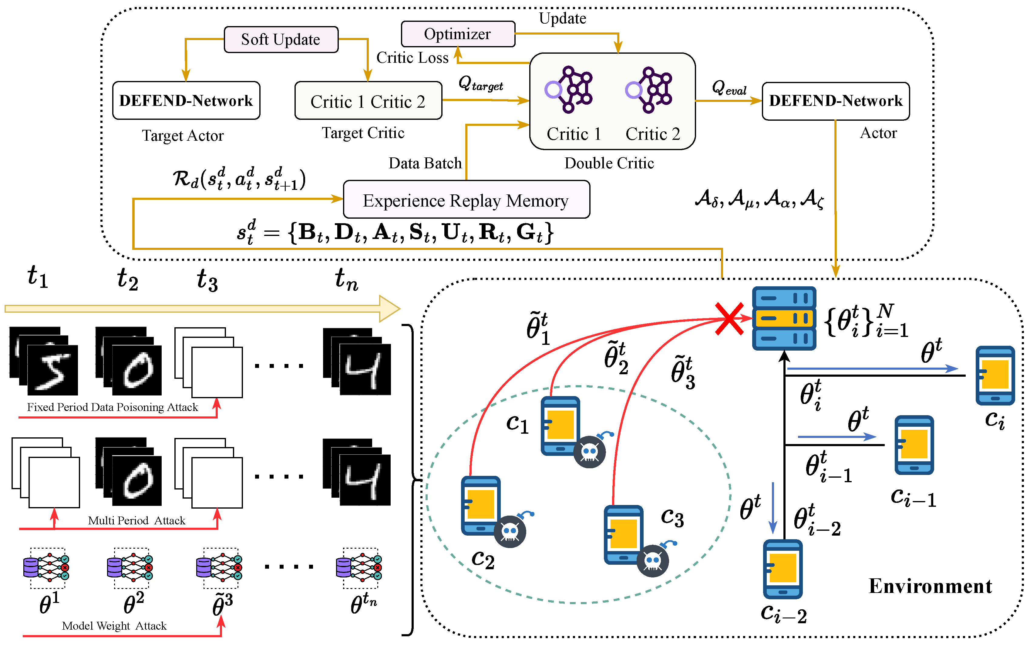
Figure 2.
Training curves of different reinforcement learning algorithms for MDP-based defense policy optimization across various network architectures and data heterogeneity levels. The curves show cumulative reward over training episodes, where represents the Dirichlet concentration parameter controlling data distribution heterogeneity (lower values indicate higher heterogeneity).
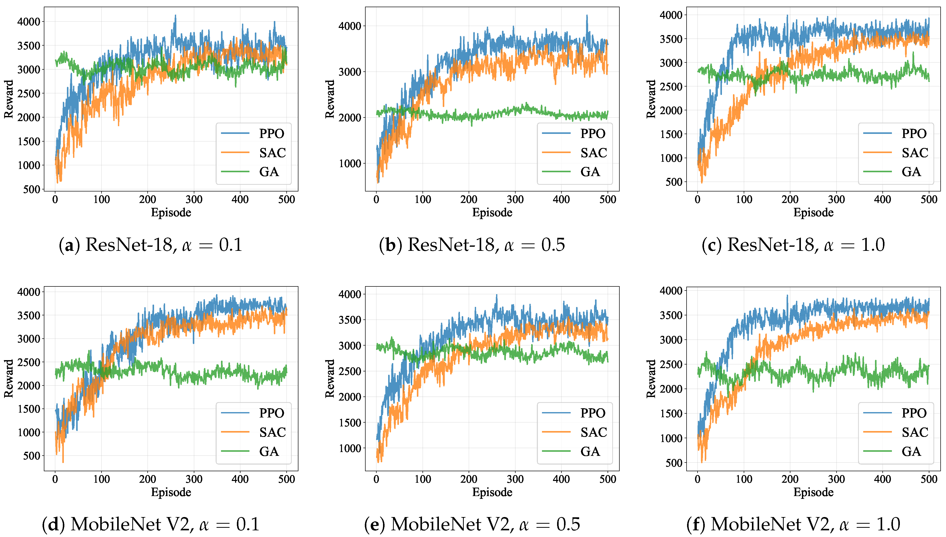
Figure 3.
Clean accuracy under defense performance comparison across different reinforcement learning algorithms, network architectures, and data heterogeneity levels. The curves demonstrate each algorithm’s ability to preserve model utility for legitimate classification tasks while actively defending against temporal backdoor attacks during training.
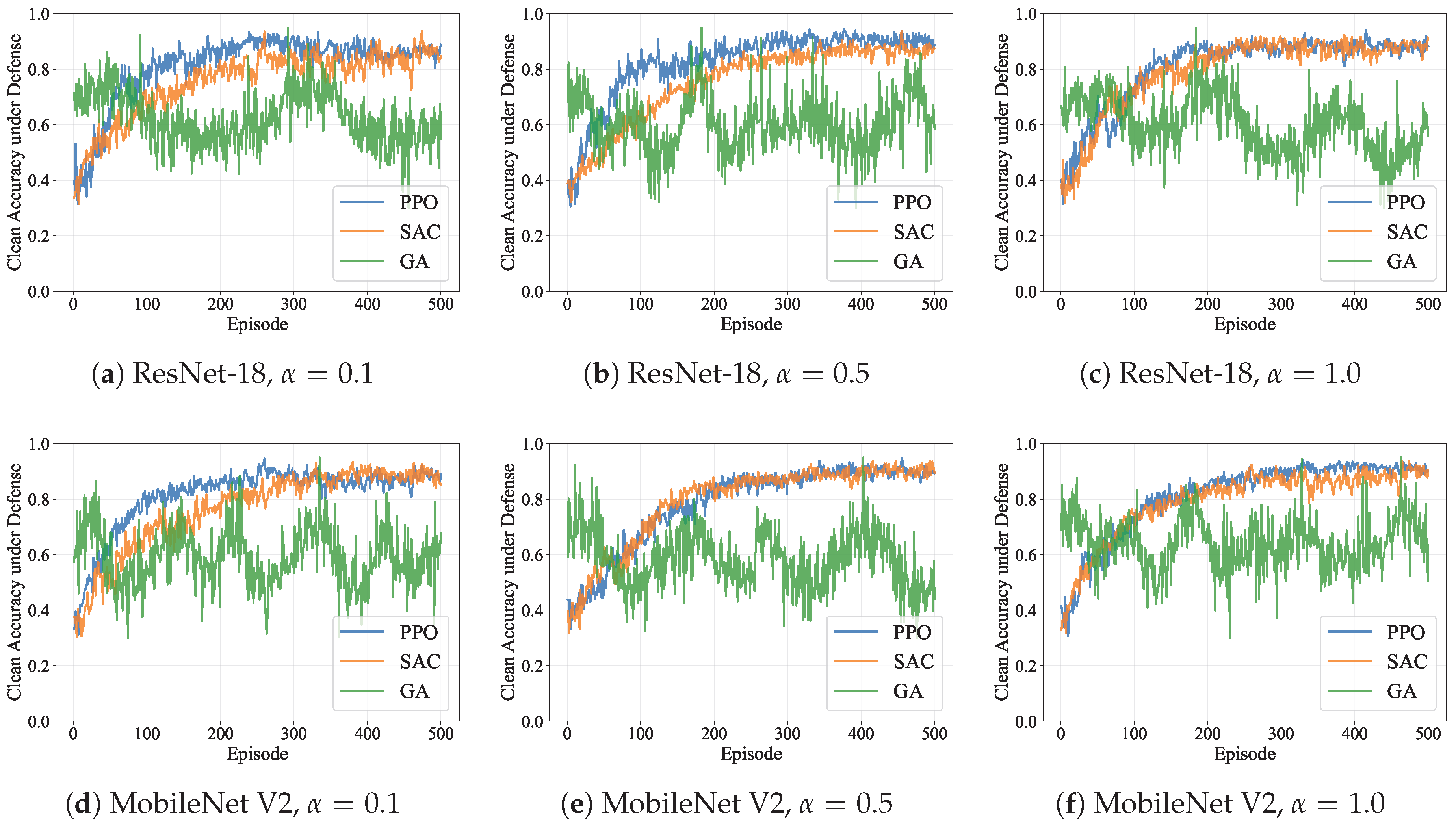
Table 2.
Experimental Parameters and Configuration Settings.
| Parameter | Symbol | Value |
|---|---|---|
| Dataset and Client Configuration | ||
| Datasets | – | CIFAR-10, FEMNIST, MNIST |
| Number of clients | N | 10, 20, 30, 40, 50 |
| Data distribution | – | Non-IID |
| Dirichlet concentration | 0.1, 0.5, 1.0 | |
| Malicious client ratio | 0.1, 0.2, 0.3, 0.4 | |
| Model architecture | – | MobileNet V2, ResNet-18 |
| Federated Learning Parameters | ||
| Learning rate | 0.01 | |
| Local epochs | – | 5 |
| Communication rounds | T | 100 |
| Batch size | – | 32 |
| Poisoning ratio | 0.1 | |
| Defense Framework Parameters | ||
| Short window size | 5 | |
| Long window size | 10 | |
| Detection threshold | 0.8 | |
| Temporal regularization | 0.1 | |
| Pattern templates | 10 | |
| Geometric median tolerance | ||
| Reputation decay scales | 3 | |
| MDP and Reinforcement Learning Parameters | ||
| Discount factor | 0.95 | |
| Policy learning rate | – | 0.001 |
| Training episodes | – | 500 |
| Max steps per episode | – | 1000 |
| Exploration rate | 0.1 | |
| Experience buffer size | – | 10,000 |
| Target network update | – | 1000 steps |
| Minimum participation | ||
Table 3.
Defense Success Rate for ResNet-18 under varying client numbers and data heterogeneity ( = 0.2).
Table 3.
Defense Success Rate for ResNet-18 under varying client numbers and data heterogeneity ( = 0.2).
| N | |||
|---|---|---|---|
| 10 | 0.847 ± 0.023 | 0.892 ± 0.019 | 0.924 ± 0.015 |
| 20 | 0.863 ± 0.021 | 0.906 ± 0.017 | 0.938 ± 0.013 |
| 30 | 0.871 ± 0.019 | 0.915 ± 0.016 | 0.947 ± 0.012 |
| 40 | 0.876 ± 0.018 | 0.921 ± 0.015 | 0.952 ± 0.011 |
| 50 | 0.879 ± 0.017 | 0.925 ± 0.014 | 0.956 ± 0.010 |
Table 4.
Temporal Detection Efficiency for ResNet-18 under varying client numbers and data heterogeneity ( = 0.2).
Table 4.
Temporal Detection Efficiency for ResNet-18 under varying client numbers and data heterogeneity ( = 0.2).
| N | |||
|---|---|---|---|
| 10 | 0.673 ± 0.041 | 0.721 ± 0.038 | 0.768 ± 0.033 |
| 20 | 0.695 ± 0.039 | 0.742 ± 0.035 | 0.789 ± 0.031 |
| 30 | 0.708 ± 0.037 | 0.755 ± 0.033 | 0.802 ± 0.029 |
| 40 | 0.716 ± 0.036 | 0.763 ± 0.032 | 0.811 ± 0.028 |
| 50 | 0.721 ± 0.035 | 0.769 ± 0.031 | 0.817 ± 0.027 |
Table 5.
Defense Success Rate for ResNet-18 under varying client numbers and malicious ratios ( = 0.5).
Table 5.
Defense Success Rate for ResNet-18 under varying client numbers and malicious ratios ( = 0.5).
| N | ||||
|---|---|---|---|---|
| 10 | 0.943 ± 0.012 | 0.892 ± 0.019 | 0.834 ± 0.026 | 0.768 ± 0.032 |
| 20 | 0.957 ± 0.011 | 0.906 ± 0.017 | 0.847 ± 0.024 | 0.781 ± 0.030 |
| 30 | 0.964 ± 0.010 | 0.915 ± 0.016 | 0.856 ± 0.023 | 0.791 ± 0.029 |
| 40 | 0.969 ± 0.009 | 0.921 ± 0.015 | 0.863 ± 0.022 | 0.798 ± 0.028 |
| 50 | 0.972 ± 0.009 | 0.925 ± 0.014 | 0.867 ± 0.021 | 0.803 ± 0.027 |
Table 6.
Temporal Detection Efficiency for ResNet-18 under varying client numbers and malicious ratios ( = 0.5).
Table 6.
Temporal Detection Efficiency for ResNet-18 under varying client numbers and malicious ratios ( = 0.5).
| N | ||||
|---|---|---|---|---|
| 10 | 0.825 ± 0.028 | 0.721 ± 0.038 | 0.612 ± 0.045 | 0.498 ± 0.052 |
| 20 | 0.841 ± 0.026 | 0.742 ± 0.035 | 0.634 ± 0.042 | 0.521 ± 0.049 |
| 30 | 0.852 ± 0.025 | 0.755 ± 0.033 | 0.649 ± 0.040 | 0.537 ± 0.047 |
| 40 | 0.859 ± 0.024 | 0.763 ± 0.032 | 0.658 ± 0.039 | 0.547 ± 0.046 |
| 50 | 0.864 ± 0.023 | 0.769 ± 0.031 | 0.664 ± 0.038 | 0.554 ± 0.045 |
Table 7.
Defense Success Rate for MobileNet V2 under varying client numbers and data heterogeneity ( = 0.2)
Table 7.
Defense Success Rate for MobileNet V2 under varying client numbers and data heterogeneity ( = 0.2)
| N | |||
|---|---|---|---|
| 10 | 0.821 ± 0.025 | 0.869 ± 0.021 | 0.908 ± 0.017 |
| 20 | 0.836 ± 0.023 | 0.883 ± 0.019 | 0.921 ± 0.015 |
| 30 | 0.845 ± 0.022 | 0.892 ± 0.018 | 0.930 ± 0.014 |
| 40 | 0.851 ± 0.021 | 0.898 ± 0.017 | 0.936 ± 0.013 |
| 50 | 0.855 ± 0.020 | 0.902 ± 0.016 | 0.940 ± 0.012 |
Table 8.
Temporal Detection Efficiency for MobileNet V2 under varying client numbers and data heterogeneity ( = 0.2)
Table 8.
Temporal Detection Efficiency for MobileNet V2 under varying client numbers and data heterogeneity ( = 0.2)
| N | |||
|---|---|---|---|
| 10 | 0.657 ± 0.043 | 0.703 ± 0.040 | 0.751 ± 0.036 |
| 20 | 0.678 ± 0.041 | 0.724 ± 0.038 | 0.772 ± 0.034 |
| 30 | 0.691 ± 0.039 | 0.737 ± 0.036 | 0.785 ± 0.032 |
| 40 | 0.699 ± 0.038 | 0.745 ± 0.035 | 0.793 ± 0.031 |
| 50 | 0.704 ± 0.037 | 0.751 ± 0.034 | 0.799 ± 0.030 |
Table 9.
Defense Success Rate for MobileNet V2 under varying client numbers and malicious ratios ( = 0.5).
Table 9.
Defense Success Rate for MobileNet V2 under varying client numbers and malicious ratios ( = 0.5).
| N | ||||
|---|---|---|---|---|
| 10 | 0.926 ± 0.014 | 0.869 ± 0.021 | 0.807 ± 0.028 | 0.739 ± 0.035 |
| 20 | 0.940 ± 0.013 | 0.883 ± 0.019 | 0.821 ± 0.026 | 0.753 ± 0.033 |
| 30 | 0.947 ± 0.012 | 0.892 ± 0.018 | 0.831 ± 0.025 | 0.763 ± 0.032 |
| 40 | 0.952 ± 0.011 | 0.898 ± 0.017 | 0.838 ± 0.024 | 0.770 ± 0.031 |
| 50 | 0.955 ± 0.010 | 0.902 ± 0.016 | 0.843 ± 0.023 | 0.775 ± 0.030 |
Table 10.
Temporal Detection Efficiency for MobileNet V2 under varying client numbers and malicious ratios ( = 0.5)
Table 10.
Temporal Detection Efficiency for MobileNet V2 under varying client numbers and malicious ratios ( = 0.5)
| N | ||||
|---|---|---|---|---|
| 10 | 0.809 ± 0.030 | 0.703 ± 0.040 | 0.591 ± 0.047 | 0.474 ± 0.054 |
| 20 | 0.825 ± 0.028 | 0.724 ± 0.038 | 0.613 ± 0.045 | 0.497 ± 0.052 |
| 30 | 0.836 ± 0.027 | 0.737 ± 0.036 | 0.628 ± 0.043 | 0.514 ± 0.050 |
| 40 | 0.843 ± 0.026 | 0.745 ± 0.035 | 0.637 ± 0.042 | 0.525 ± 0.049 |
| 50 | 0.848 ± 0.025 | 0.751 ± 0.034 | 0.644 ± 0.041 | 0.533 ± 0.048 |
Disclaimer/Publisher’s Note: The statements, opinions and data contained in all publications are solely those of the individual author(s) and contributor(s) and not of MDPI and/or the editor(s). MDPI and/or the editor(s) disclaim responsibility for any injury to people or property resulting from any ideas, methods, instructions or products referred to in the content. |
© 2025 by the authors. Licensee MDPI, Basel, Switzerland. This article is an open access article distributed under the terms and conditions of the Creative Commons Attribution (CC BY) license (http://creativecommons.org/licenses/by/4.0/).
Copyright: This open access article is published under a Creative Commons CC BY 4.0 license, which permit the free download, distribution, and reuse, provided that the author and preprint are cited in any reuse.


