
Submitted:
01 October 2025
Posted:
02 October 2025
You are already at the latest version
Abstract
Vector-Symbolic Architectures (VSAs) provide a powerful, brain-inspired framework for representing and manipulating complex data across the biomedical sciences. By mapping heterogeneous information, from genomic sequences and molecular structures to clinical records and medical images, into a unified high-dimensional vector space, VSAs enable robust reasoning, classification, and data fusion. Despite their potential, the practical design and implementation of an effective VSA can be a significant hurdle, as optimal choices depend heavily on the specific scientific application. This article bridges the gap between theory and practice by presenting ten tips for designing VSAs tailored to key challenges in the biomedical sciences. We provide concrete, actionable guidance on topics such as encoding sequential data in genomics, creating holistic patient vectors from electronic health records, and integrating VSAs with deep learning models for richer image analysis. Following these tips will empower researchers to avoid common pitfalls, streamline their development process, and effectively harness the unique capabilities of VSAs to unlock new insights from their data.
Keywords:
hyperdimensional computing
; vector-symbolic architectures
; biomedical sciences
; tips and pitfalls
; biomedical data
Introduction
Imagine trying to describe every person you know using only three attributes: height, weight, and age. While useful, this system quickly fails. Two very different people might have similar values, and complex traits like personality or relationships are impossible to capture. Now, imagine you could use 10,000 different attributes. In this vast feature space, every individual would have a unique, rich description, and we could represent relationships through mathematical combinations of these descriptions. This is the core idea behind Hyperdimensional Computing (HDC) [1,2].
Also known as Vector-Symbolic Architectures (VSAs), HDC is a brain-inspired computational framework that represents and processes information in a fundamentally different way from traditional computing. HDC operates on high-dimensional vectors, or hypervectors, as long list of numbers (often 1,000 to 10,000+). These vectors are often implemented with bipolar scalars (+1, -1) distributed through the 1-dimensional structure. In this paradigm, a hypervector is not just a point in space. It is a holistic and distributed representation of a concept.
The power of HDC emerges from a small yet capable set of mathematical operations used to combine symbolic vectors; collectively they are known as the MAP (Multiply-Add-Permute) model:
- Binding (element-wise multiplication, ⊗): links two concepts represented in the vectors together. For example, binding the vector representation of the concept serum level with the vector representation of the concept high creates a new, distinct hypervector representing the composite idea high serum level;
- Bundling (element-wise addition, ⊕): combines multiple concepts in vector format. One could bundle the vectors for high serum glucose, high blood pressure, and patient ID: 123 to create a single vector representing a patient’s state. This operation highlights a key property of HDC: the ability to easily integrate heterogeneous information, numerical values, categorical states, or identifiers, into one coherent data structure;
- Permutation (rotation, ρ): encodes order of sequences, which is critical for representing sequential data like DNA strands or time-series events in a patient’s record. In this operation, each hypervector is shifted or rotated according to its position in the sequence, ensuring that the same concept appearing at different positions is represented uniquely. This positional encoding preserves order while keeping the representations nearly orthogonal, thereby allowing clear distinction between sequences and their components.
This approach yields remarkable properties. Because information is distributed across thousands of components, HDC models are inherently robust to noise and errors (flipping a few values in a hypervector does not meaningfully change the concept it represents; much like how the brain can function despite the loss of individual neurons) [3,4]. Furthermore, these models are computationally efficient and excel at one-shot or few-shot learning, enabling rapid model training from very little data [5,6,7,8].
Given its unique strengths, HDC is poised to address some of the most pressing challenges in the biomedical sciences [9,10]. To help researchers harness its potential, this article offers ten practical tips for designing and implementing these powerful architectures for your own research challenges. Rather than providing generic advice, the tips are structured around specific applications, offering tailored guidance for distinct problems, from analyzing genomic sequences and processing clinical records to interpreting medical images. This application-driven approach, illustrated schematically in Figure 1, provides a clear roadmap for using HDC to solve real-world challenges in computational biology and medicine. Finally, to make this effort truly hands-on, each tip is accompanied, where applicable, by practical examples using the hdlib Python library [11]. For self-contained concepts, we provide ready-to-use code, while for more complex scenarios involving technologies outside the scope of this article, we use structured pseudocode to illustrate the core logic.
Tip 1: For Electronic Health Records – Use Bundling to Create Holistic Patient Vectors
Electronic Health Records (EHRs) are a goldmine of information, but they are notoriously complex and messy [12]. A single patient’s record is a patchwork of different data types: structured codes for diagnoses and billing, numerical values for lab results, text from clinical notes, and lists of prescribed medications. For unstructured sources like clinical notes, Natural Language Processing techniques can first be employed to extract key symbolic entities that are then encoded using VSA [13,14,15]. Crucially, this data is almost always incomplete [16,17]. One patient might have a full panel of recent lab work, while another might have none. Traditional machine learning models often struggle with this kind of sparse, heterogeneous data, typically requiring complex preprocessing and imputation to fill in the missing values [18,19,20].
HDC offers an elegant solution through the bundling operation, which is almost always a simple vector addition. The core idea is to create a single, holistic hypervector for each patient that acts like a summary of all their known information. This patient vector is not sensitive to what is not in the summary. It just represents the sum of what is. This approach is incredibly robust to missing data and naturally integrates different information types into one unified representation [21].
How to Create a Patient Vector
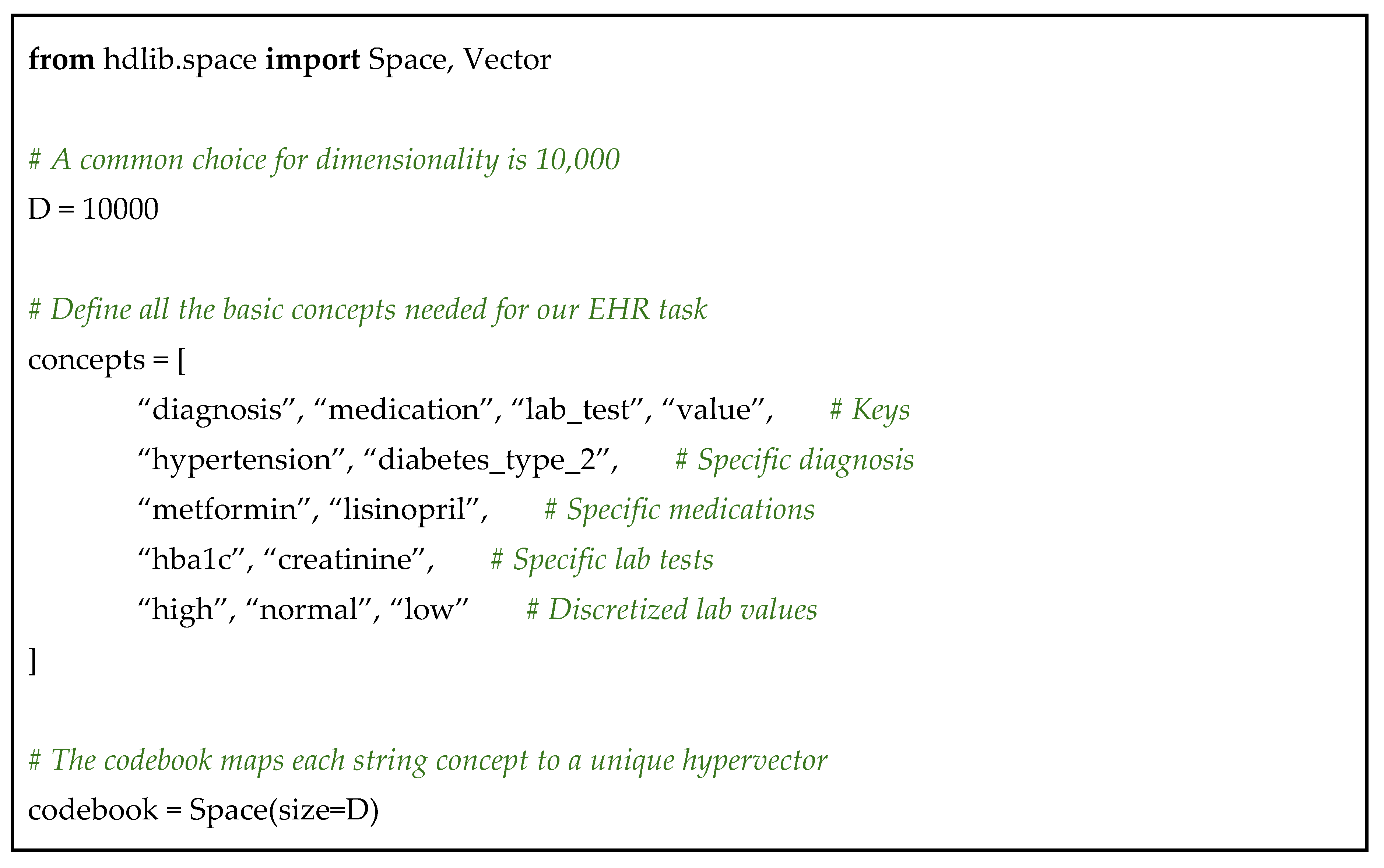
First, you need a dictionary that maps every elementary piece of information to its own unique and random 1-dimensional vector in 10,000 size. This is your codebook. Your atomic concepts would include:
- Keys for data types: diagnosis, medication, lab_test, value;
- Specific diagnose: diabetes_type_2, hypertension;
- Specific medications: metformin, lisinopril;
- Specific lab tests: hba1c, creatinine;
- Discretized lab values: high, normal, low.
Using hdlib, we can create this with a simple list of concepts, as shown in Code 1 below.
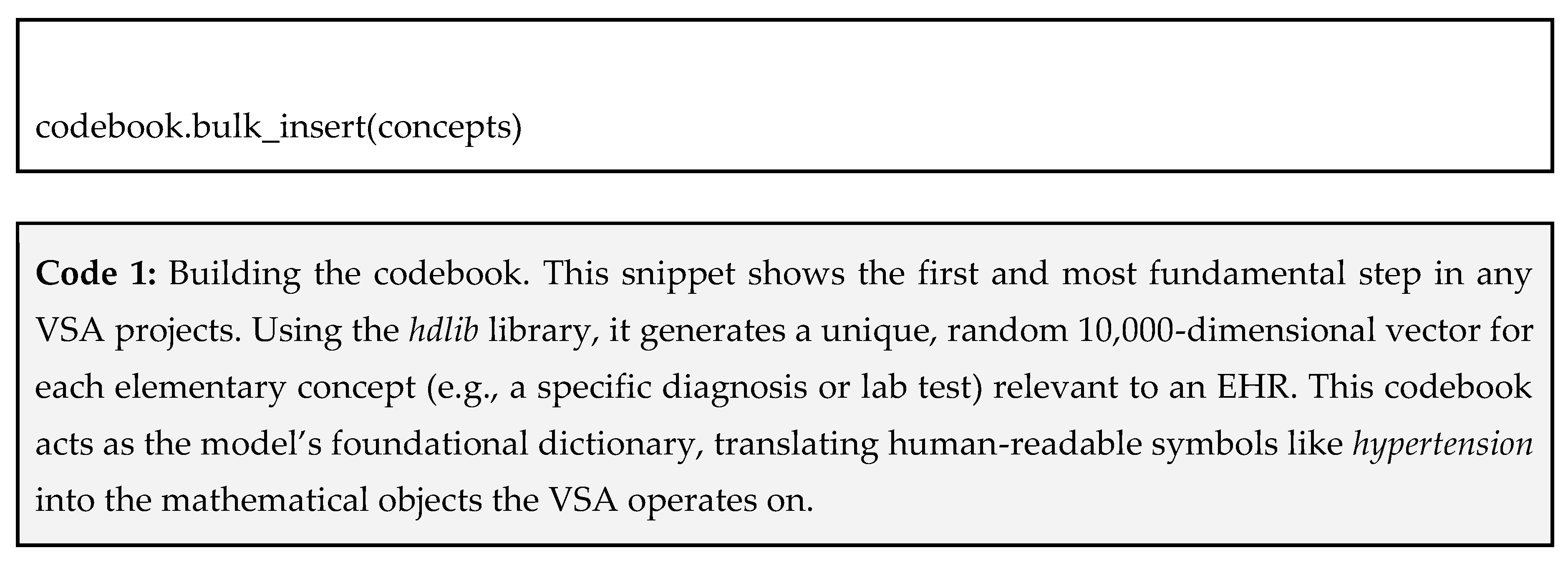
For each piece of information in a patient's record, you can create a vector by binding the key to its value. Binding combines them to create a new, distinct product vector that is dissimilar to its original components:
- A diagnosis of hypertension becomes: patient_diagnosis = diagnosis ⊗ hypertension
- A prescription for metformin becomes: patient_prescription = medication ⊗ metformin
- A HbA1c result of 8.1% (which we categorize as high) becomes: patient_hba1c = (lab_test ⊗ hba1c) ⊕ (value ⊗ high)
Notice that we bundled two bound pairs to represent a more complex fact (the test and its result)
This translates to the following code using hdlib (Code 2).
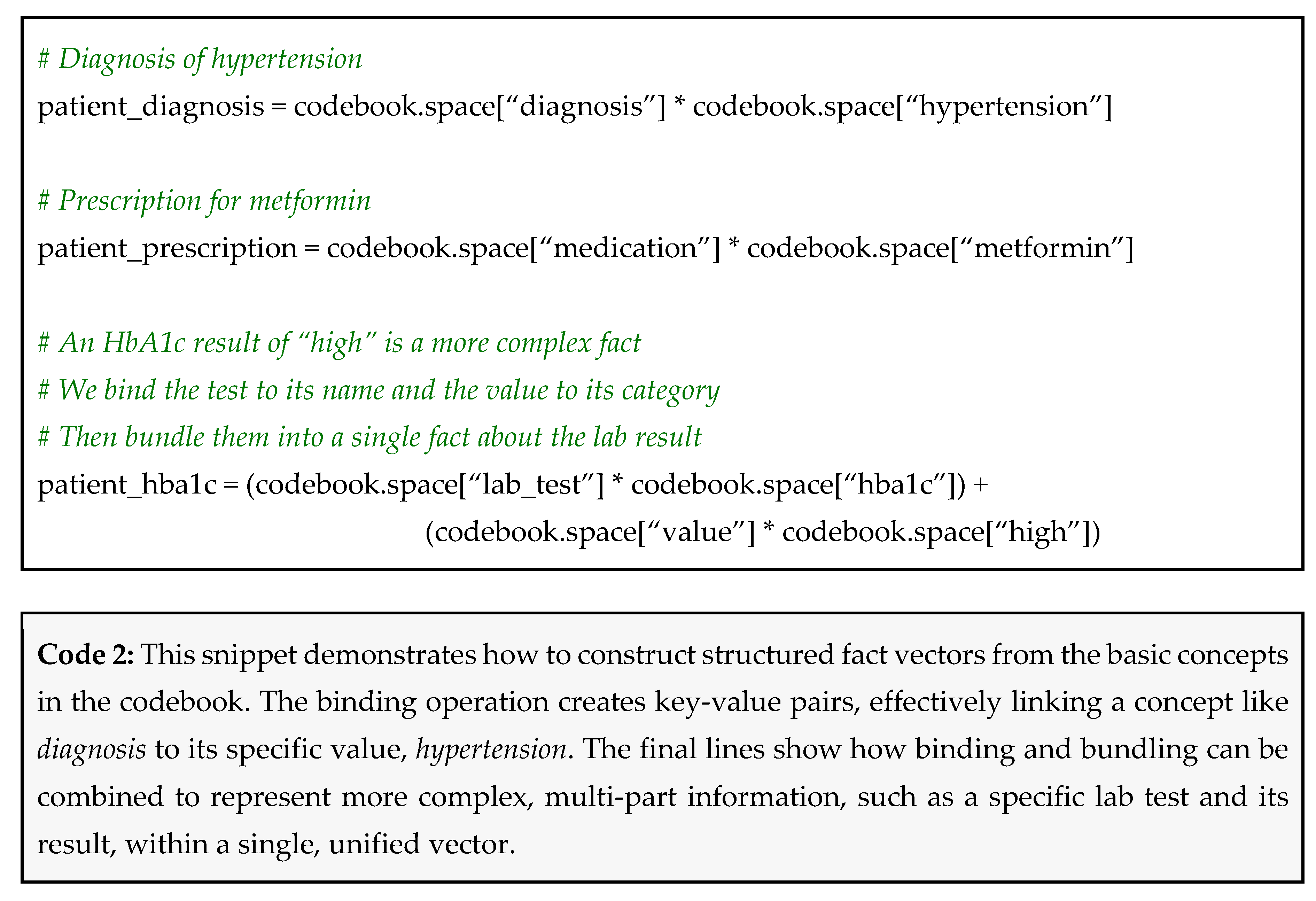
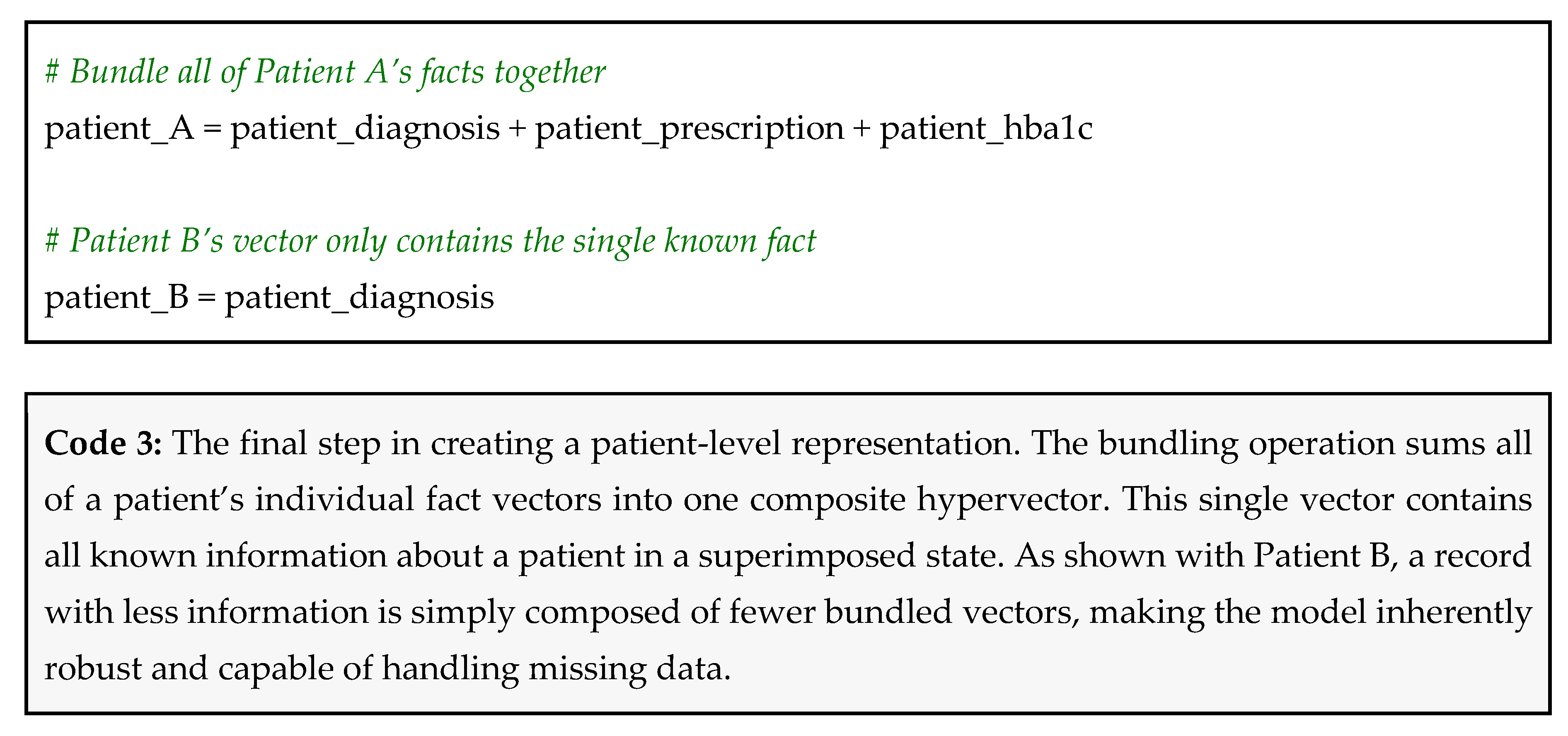
Now, you simply bundle all of a patient’s fact vectors together to create their final, comprehensive representation.
Let’s consider Patient A: high hypertension, takes metformin, has high HbA1c. Their patient vector would be calculated as:
patient_A = (diagnosis ⊗ hypertension) ⊕ (medication ⊗ metformin) ⊕ ((lab_test ⊗ hba1c) ⊕ (value ⊗ high))
Now, consider Patient B, for whom we only have a diagnosis: has hypertension. Their vector is simply:
patient_B = diagnosis ⊗ hypertension
This can be simply achieved using hdlib as shown in Code 3.
Why This Works
- Robustness to missing data: Patient A’s vector was created without knowing their creatinine level. Patient B’s vector was created with only one piece of information. The model does not break or require modification. It works with whatever data is available [4];
- Similarity-based reasoning: the magic happens when you compare patient vectors. The vector for Patient B is a component of the vector for Patient A. Mathematically, this means that their two vectors have a high degree of similarity. Thus, in general, you can find patients with similar clinical profiles by simply looking for vectors having high cosine similarity. Note that hdlib provides a dist function as Vector’s instance method to perform the cosine distance between the specific instance vector and a different Vector object, defined as 1 minus the cosine similarity. Following the previous example shown in Code 3, we can compute the cosine distance between patient_A and patient_B vectors using hdlib as: patient_A.dist(patient_B, method=“cosine”) [24].
There are however a couple of pitfalls that you should be careful of while creating holistic patient vectors:
Pitfall 1: unbalanced feature influence – if one type of data has far more entries per patient than another, simply summing them can create a patient vector that is dominated by the more frequent data type. For instance, the model might become great at seeing lab patterns but blind to diagnoses.
How to avoid pitfall 1: normalize by feature type – before bundling, you can create sub-vectors for each category. Normalize these sub-vectors so they have a magnitude of 1, and then bundle the normalized sub-vectors. This ensures each data modality contributes equally to the final patient vector, regardless of the number of entries.
Pitfall 2: over-discretization of numerical values – when converting a continuous value like blood pressure into a symbolic vector (e.g., high, normal, low), choosing poor thresholds can lose critical information. A patient with a value just barely in the normal range might be treated the same as one with a perfect value.
How to avoid pitfall 2: use fractional binding or more granular categories – instead of just high, consider multiple levels like normal, elevated, hypertension_stage_1.
Tip 2: For Genomics and Proteomics – Leverage Permutations to Encode Sequences
In genomics and proteomics, the order of elements defines function. For example, the DNA sequence ACG (encoding the aminoacid Threonine) is fundamentally different from GCA (Alanine), even though they contain the exact same nucleotides. A model that cannot distinguish ACG from GCA is useless for most bioinformatics tasks.
Encoding Positions
HDC solves this problem using the positional vector binding or the permutation operator . Permutation systematically shuffles the elements of a hypervector in a deterministic way. For example, a single permutation might rotate the vector’s 10,000 elements one position to the left. Applying it again rotates it one more position. Each amount of shift represents a specific location in a sequence, thereby preserving positional information during encoding. Crucially, each permutation creates a new hypervector that is dissimilar (quasi-orthogonal) to the original and to other permutations of itself. This property allows us to encode an element’s relative position within a sequence [25,26,27]. On the other hand, positional binding with separate vectors assigned to specific positions is another approach. In this method, each position (symbolic information) is represented by a unique hypervector. Let’s explore the two primary ways to do this:
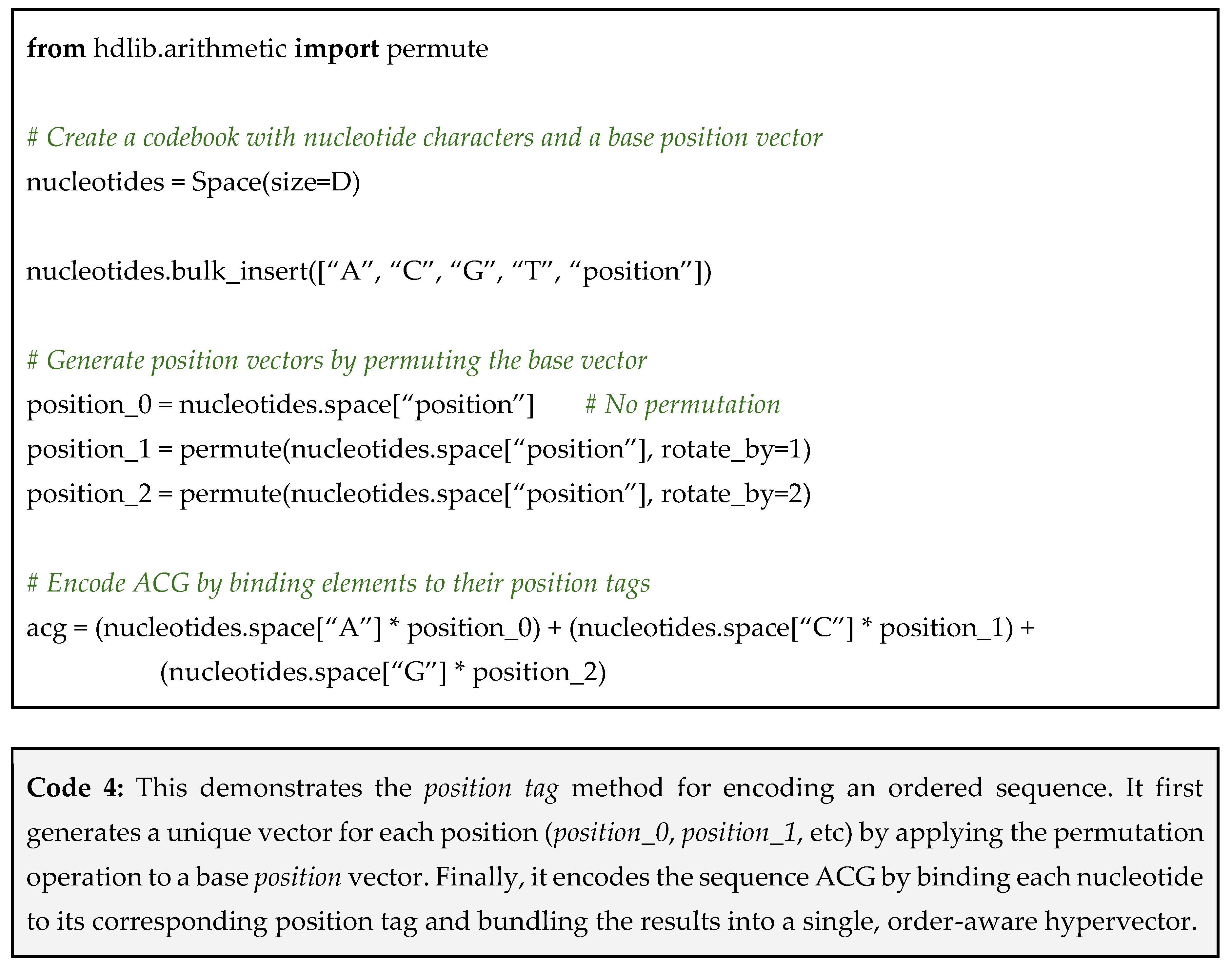
Method 1: binding with a position vector – This method is like putting labeled tags on items. You create a generic position vector and permute it to create a unique tag for each position (position_0, position_1, position_2). You then bind each sequence element to its corresponding position tag. This method is best suitable for answering the question “what is at a specific position?”. This can be easily achieved using hdlib as in Code 4.
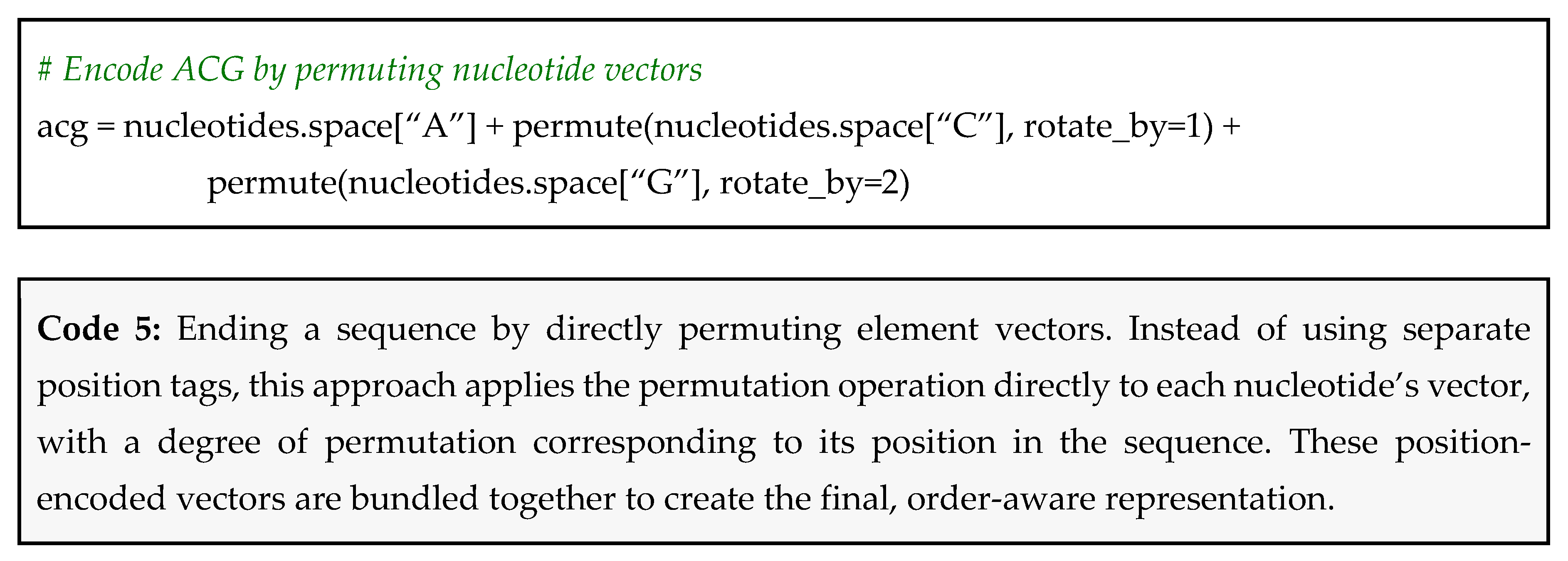
Method 2: directly permuting element vectors – This more direct method alters the element’s vector itself based on its position. The first element’s vector is permuted 0 times, the second is permuted once, the third twice, and so on. This is best for answering the question “where is a specific element?”. A Python snippet using hdlib is reported in Code 5.
Returning to the example of ACG and GCA; when encoding ACG by permuting approach, the vector for A is left unshifted for the first position, while C and G are permuted by one and two positions, respectively, before binding and bundling into a single representation. For GCA, the vector for G remains unshifted, while C and A are permuted by one and two positions, respectively. As a result, even though both sequences contain the same symbols, their encodings yield distinct hypervectors, preserving order information.
Furthermore, this encoding can be extended to capture higher-level biological knowledge, such as the codon wobble base phenomenon. By bundling the sequence vector of a codon with the vector for the amino acid it encodes, we can create biologically-aware representations. In this model, vectors for synonymous codons (e.g., GCA and GCC) become highly similar, as they share the same core amino acid vector, while vectors for non-synonymous codons remain dissimilar. This demonstrates how VSAs can move beyond literal sequence representation to encode abstract functional relationships.
Which Method Should You Choose?
For general sequence comparison, both methods are equally effective. They both successfully create distinct, dissimilar vectors for sequences with different orderings.
The choice depends on the specific questions you want to ask your model:
- Choose method 1 if your primary task is querying by position. For instance, if you frequently need to ask questions like “what nucleotide is at position 257?”, method 1 excels because you can directly query the full sequence vector with the position_257 vector to retrieve the answer;
- Choose method 2 if your goal is general sequence comparison, alignment, or if you need to ask questions like “at what positions does Adenine (“A”) appear?”. This approach is more elegant and memory efficient and requires a smaller codebook.
It should also be noted that repeatedly permuting a hypervector to represent many positions may eventually be limited by the vector size. When symbolic position information spans many locations, Method 1 can be a better option, since randomly generated position vectors are guaranteed to be quasi-orthogonal, avoiding the potential for cyclical collisions that can occur with repeated permutations.
Pitfall: boundary crosstalk – when you encode a very long sequence, the permutations can become so extensive that the vector for position 1,000 might, by chance, become similar again to the vector for position 10. This is called crosstalk and can corrupt the positional information.
How to avoid the pitfall: use hierarchical encoding – instead of encoding a several thousands base-pair genome as a one monolithic vector, break it down. Create a vector for each gene, then bundle the gene vectors to create a vector for a chromosome, and finally bundle chromosome vectors for the genome. This chunking contains the permutations within smaller, more manageable contexts (e.g., position is relative to the start of the gene, not the chromosome).
Tip 3: For Medical Imaging – Combine Vector-Symbolic Architectures with Convolutional Neural Networks for Explicable Artificial Intelligence
Convolutional Neural Networks (CNNs) are incredibly powerful for medical image analysis. They can classify tumors, spot anomalies, and segment organs with remarkable accuracy [28,29,30,31,32]. However, they have a major drawback: they are often black boxes. A CNN might correctly classify a histology slide as malignant, but it cannot easily explain why. It cannot answer a doctor’s follow-up questions like “which region of the image led to this conclusion?” or “what specific cellular structures did you find?”. This lack of interpretability is a significant barrier to trust and adoption in clinical settings.
Building a Queryable Scene Description
Instead of replacing CNNs, we can augment them with VSAs to create a hybrid, explainable AI model. Think of it like a two-part team:
- CNN acts as a junior technician. It has incredible eyes and can spot thousands of tiny, low-level patterns (textures, edges, shapes) in an image but cannot articulate what they mean;
- VSA acts as a senior pathologist. It takes the technician’s findings, gives them symbolic names (e.g., “spindle-shaped cells”, “high nuclear density”), notes their locations, and assembles everything into a structured, queryable report.
This hybrid model gives you the best of both worlds: the pattern-recognition power of deep learning and the reasoning and interpretability of symbolic architectures [33,34,35].
Because a full implementation is highly complex, we will use a mix of descriptive steps and pseudocode to illustrate the logic:
Step 1: divide the image and extract features with a CNN – First, we break the input image (e.g., a large histology slide) into a grid of smaller patches (e.g., 16x16 grid). We then feed each patch into a pre-trained CNN. Instead of using the CNN’s final classification, we intercept the output from an earlier layer, a rich feature vector that numerically describes the contents of that path. As anticipated earlier, since the implementation of this step could involve getting deep into many details about neural networks in general, we are going to assume that this method is implemented in a function called cnn_feature_extractor that, given an image patch, returns the feature vector;
Step 2: build a VSA codebook for features and locations – Next, we create a VSA codebook to hold the symbolic representations of the image’s contents. This involves two sets of concepts: vectors for each spatial location in our grid, and vectors for the low-level features the CNN finds. Since we do not know what the raw numerical features from the CNN mean ahead of time, we must first discover and then name them. This is a two-step process:
- Discover feature groups: we first run a clustering algorithm (like K-Means) on all the feature vectors produced by the CNN from a training set of images. This groups the thousands of slightly different numerical feature vectors into a small number of distinct clusters. Each cluster represents a recurring visual pattern, like a certain texture or cell shape;
- Assign symbolic names: we then treat each cluster as a single, unified concept. We assign a symbolic name to each one and generate a unique, random hypervector for each of these symbolic names in our codebook.
The numerical cluster centroid (the average feature in a group) is only used temporarily to determine which symbolic name a new, unseen CNN feature belongs to. The VSA model itself works exclusively with the final symbolic hypervectors.
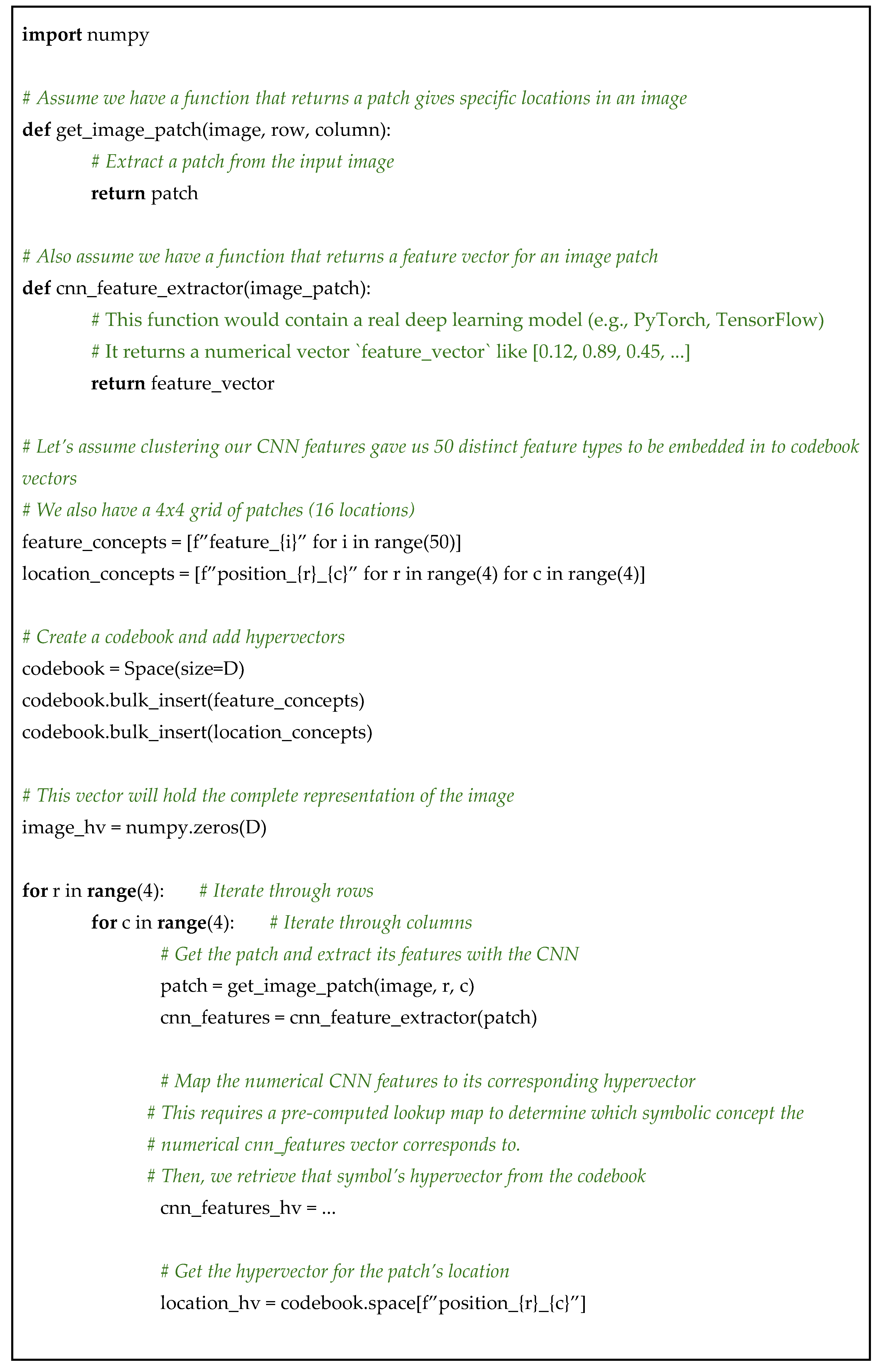
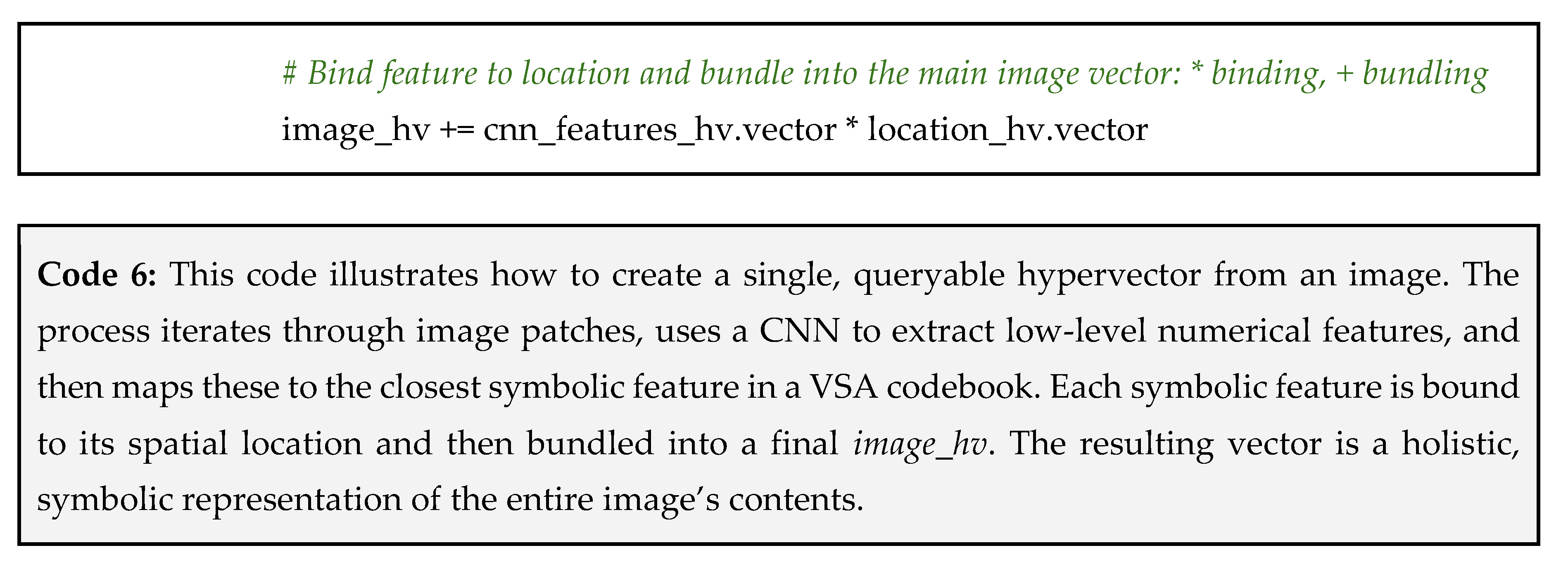
Step 3: create the composite image vector – Now, we loop through each patch of the image. For each patch, we get its CNN feature vector, find the closest matching symbolic feature in our VSA codebook, and bind that symbolic feature to the patch’s location vector. Finally, we bundle all these bound pairs into a single hypervector that represents the entire image.
The whole process is summarized in Code 6.
Why This Works
The image_hv in Code 6 is now a fully symbolic and queryable model of the image’s contents. You can interrogate it using VSA operations to ask questions that a standard CNN could never answer.
Query: “What features are present in the top-right corner (position 0, 3)?”
To answer this, we take our composite image_hv and unbind the location vector for position_0_3. In hdlib, this is done by binding, as shown in Code 7.
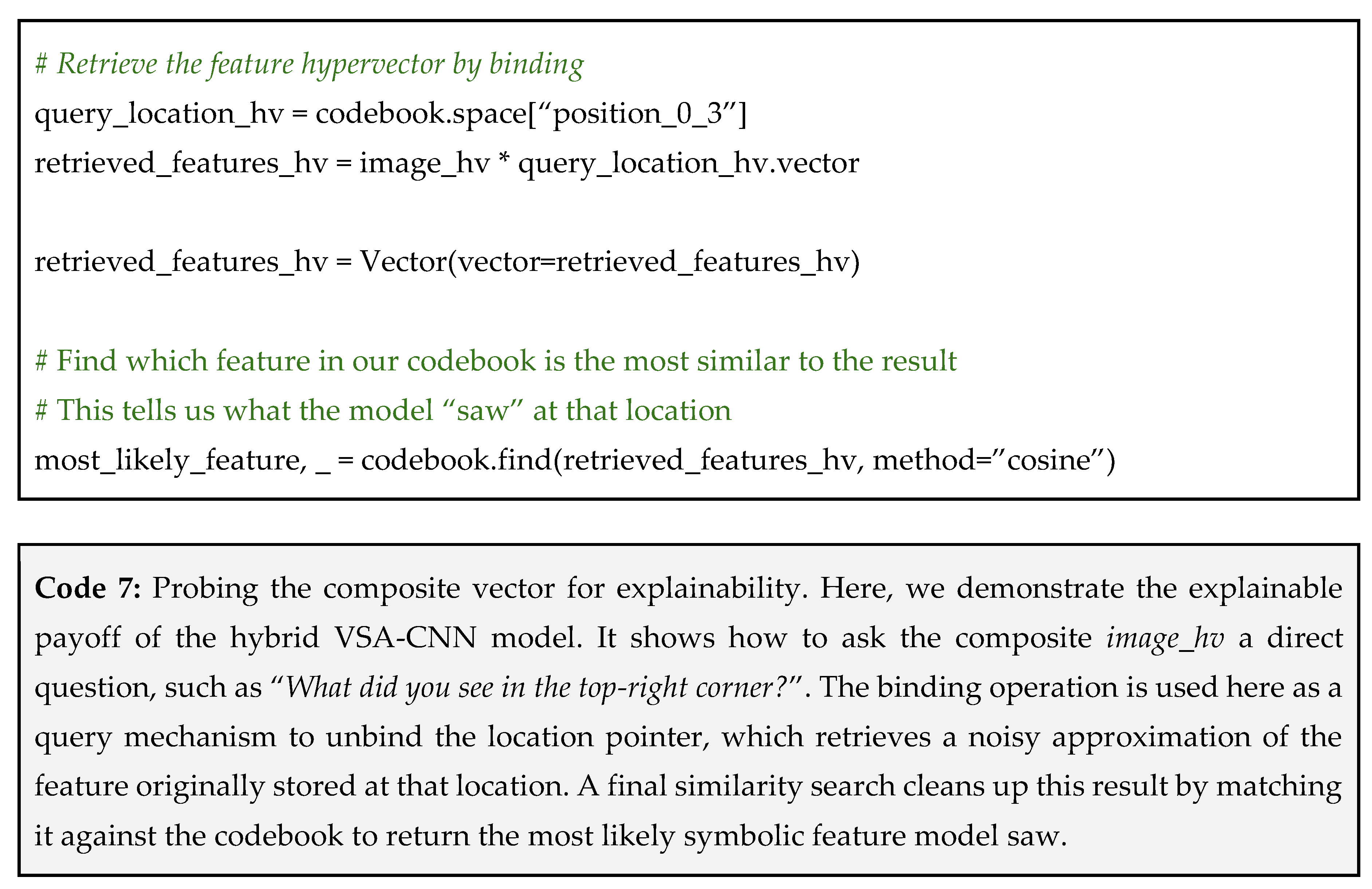
This process turns the black box into an explainable model. A doctor can now not only see the final classification but can also probe the model’s intermediate reasoning, potentially discovering novel biomarkers reflected in the learned features.
Pitfall: meaningless VSA feature codebook – if the clusters generated from the CNN’s feature vectors are not distinct or meaningful, the VSA codebook will map to noisy, overlapping concepts (e.g., feature_7 and feature_12 represent very similar patterns). The symbolic model will then be built on a faulty foundation.
How to avoid the pitfall: tune the CNN and clustering – ensure the CNN is well-trained for feature extraction. Experiment with different clustering algorithms and a varying number of clusters. Manually inspect the image patches corresponding to each cluster to see if they present visually coherent patterns. The goal is to create a VSA codebook where each feature corresponds to a recognizable visual element. Finally, remember that the quality of the VSA codebook directly affects vector generation: similar items should map to hypervectors with high correlation, while dissimilar items should map to nearly orthogonal hypervectors. This alignment ensures that symbolic reasoning is grounded in meaningful representations.
Tip 4: For Biosignal Processing (EEG/ECG) – Encode Time-Frequency Data Symbolically
Biosignals like Electroencephalograms (EEG) and Electrocardiograms (ECG) are continuous, noisy, and incredibly dense with information. A key challenge is capturing how the signal’s characteristics change over time. For EEG, a researcher is not just interested in whether alpha waves are present, but whether they are present now, in this specific region of the brain, and at what intensity. Traditional methods often struggle to represent these dynamic, multi-faceted states in a unified way, making it difficult to classify complex cognitive states or detect transient events like a seizure onset [36,37].
A Symbolic Snapshot of the Signal’s State
The VSA approach is capable of transforming the raw, numerical signal into a series of symbolic snapshots. Instead of working with the waveform directly, we first use standard signal processing techniques (like the Short-Term Fourier Transform) to analyze a short window of the signal [38]. This tells us which frequency bands (e.g., Delta, Theta, Alpha, Beta) are powerful at that time stamp. We then encode this frequency information into a single hypervector that represents the signal’s state for that specific window.
By stringing these snapshot vectors together, we can create a rich, symbolic representation of the signal’s evolution over time, perfect for classification and event detection [5,39,40,41,42,43].
Here, we are going to use a simplified EEG example, but the same logic applies to ECG, EMG, or other time-series data:
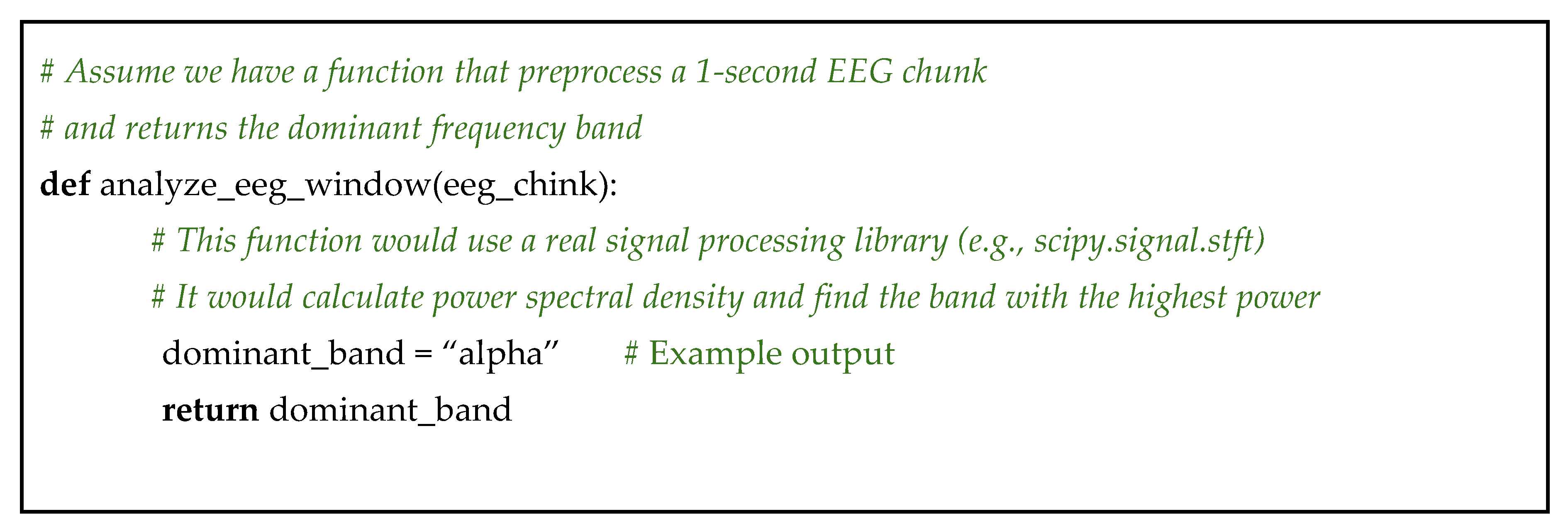
Step 1: pre-process the signal into time-frequency windows – this step does not involve VSAs. You would use a standard library like scipy [44] or mne [45] in Python to take your raw EEG signal and process it. The goal is to get the average power in each standard frequency band (Delta: 0.5–4 Hz, Alpha: 8–12 Hz, etc.) for short, overlapping time windows (e.g., 1-second windows);
Step 2: build a VSA codebook for signal features – now we create our VSA dictionary. The concepts will be the names of our frequency bands and the different brain regions (channels) from which the signal is recorded;
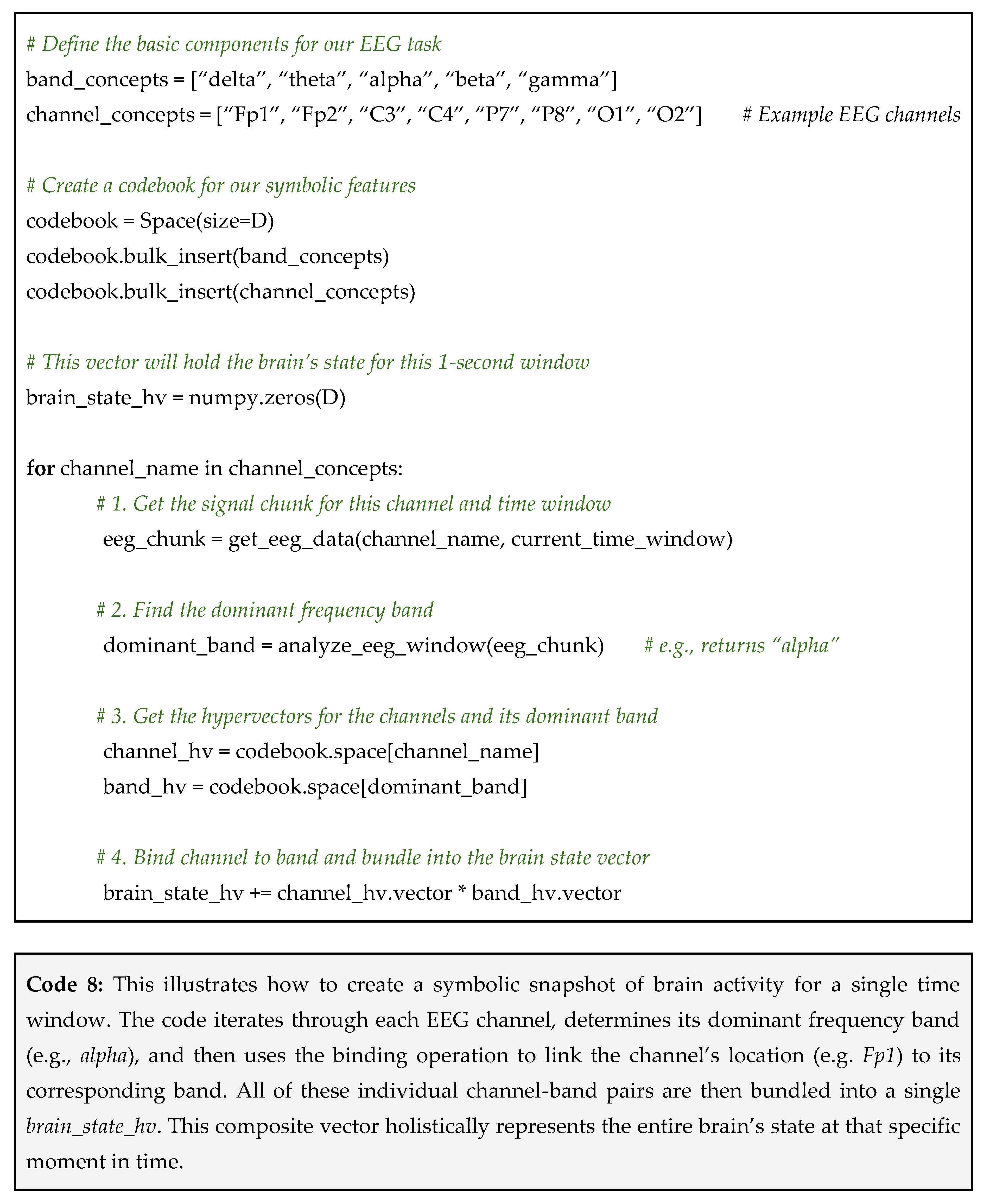
Step 3: create a composite hypervector for each time window – for each window of time, we create a single hypervector that captures the state of the entire brain. We loop through each EEG channel, find its dominant frequency band for that window, and bind the channel vector to the band vector. Then, we bundle all these bound pairs together.
This process is summarized in Code 8.
Why This Works
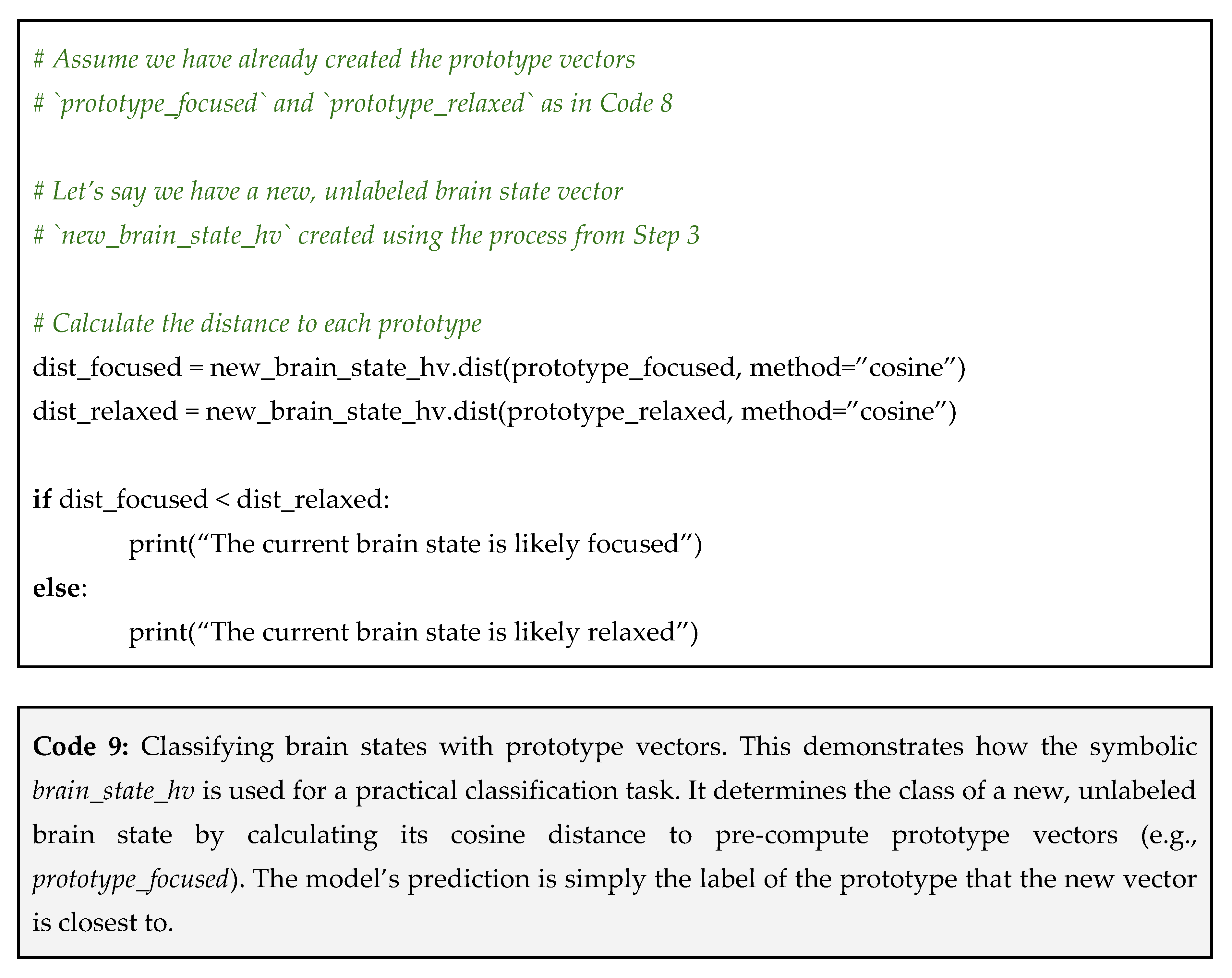
After repeating this process for many time windows, you will have a set of brain_state_hv vectors. You can now use these for high-level tasks. For example, to build a classifier for focused vs. relaxed states:
- Create a prototype: collect many brain_state_hv samples while a subject is focused and bundle them together to create a single prototype_focused vector. Do the same for the relaxed state to create prototype_relaxed;
- Classify new data: to classify a new, unseen brain_state_hv after following the same encoding steps of a single test sample, simply check whether it is more similar to the focused or relaxed prototype (see Code 9 for a pseudocode using hdlib).
This approach transforms a complex, continuous signal processing problem into a much simpler symbolic reasoning task, making it easy to build robust and transparent classifiers for dynamic biological state.
Pitfall: wrong window size – if the time window for your analysis is too short, you will not have the frequency resolution to accurately detect low-frequency bands (like Delta waves). If it is too long, you will average out rapid, transient events and miss them entirely.
How to avoid the pitfall: match the window size to the phenomenon of interest – this is a classic signal processing trade-off. If you are looking for slow-changing cognitive states, a longer window (1-2 seconds) is fine. If you are trying to detect sharp, brief events like epileptic spikes, you need a much shorter window (e.g., 100-250 milliseconds). You may even need to run your analysis in parallel with multiple window sizes to capture different types of events.
It is important to craft hypervectors independently, especially for band and channel symbols. Keep the random source separate for each symbol, and ideally for each concept, to preserve strong orthogonality (rather than merely near-orthogonality).
Tip 5: For Molecular Structures – Decompose Molecules into Atomic Fragments
A molecule’s chemical properties, like its toxicity, solubility, or ability to bind to a target protein, are determined by its 3D structure and are the arrangement of its atoms and bonds. This structure is fundamentally a graph, not a simple sequence or a fixed-size table. Representing this complex, non-linear information for machine learning is a significant challenge. How can we compare the structure of caffeine to that of aspirin in a mathematically meaningful way? Standard models often require fingerprinting methods that convert these graphs into binary vectors, but these can sometimes lose granular information [46,47,48].
A Sum of Its Parts
The VSA approach treats a molecule as a composition of its local atomic environments. Instead of trying to encode the entire molecular graph at once, we break it down into smaller, overlapping fragments. A fragment can be as simple as an atom and its immediate bonding partner. We then create a hypervector for each of these fragments and bundle them together to form a single hypervector that represents the entire molecule.
This method elegantly captures the principle that a molecule’s function is determined by the sum of its constituent chemical groups (e.g., hydroxyl groups, benzene rings). Molecules with similar functional groups will have similar hypervectors, allowing us to predict properties and behavior.
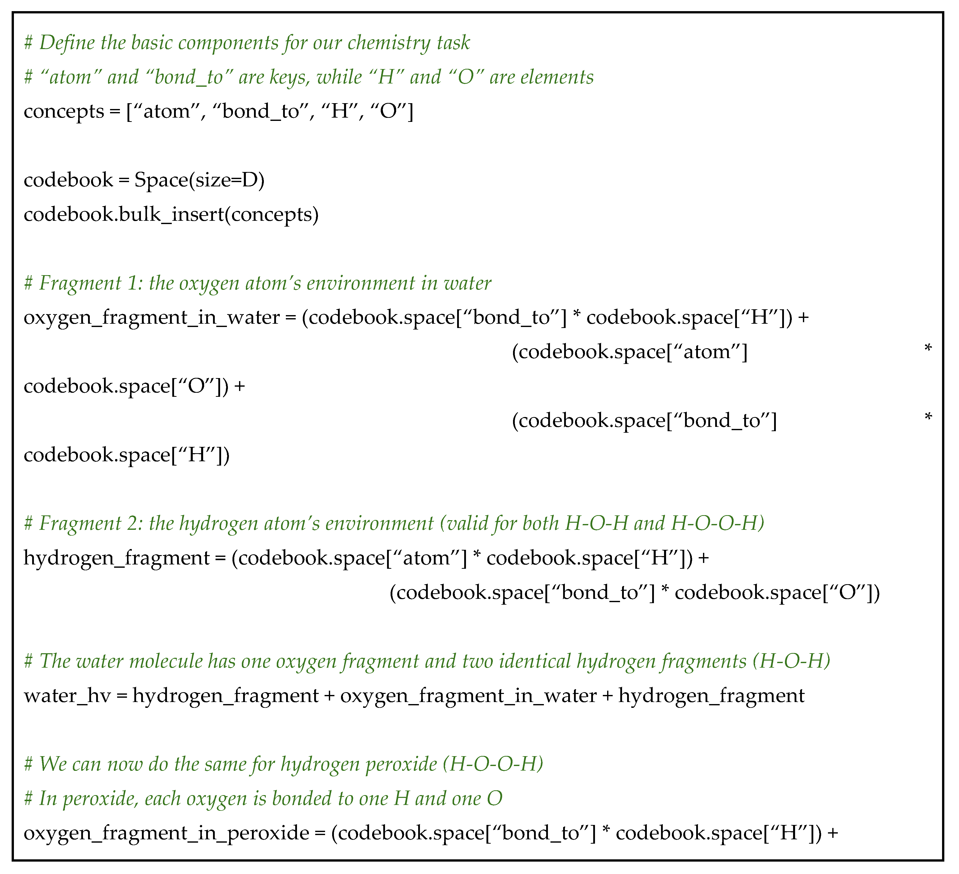
Let’s use a simplified representation of a water molecule (H-O-H) and a hydrogen peroxide molecule (H-O-O-H) to illustrate the process:
Step 1: define your atomic and bonding codebook – first, we create a VSA codebook for the basic building blocks, i.e., the different types of atoms (elements);
Step 2: define and encode atomic fragments – an atomic fragment is the local environment around a central atom. We can represent it by bundling the central atom’s vector with vectors representing each of the neighboring atoms. The fragments in a water molecule are defined as:
- o oxygen fragment: one central oxygen atom connected to two hydrogens via single bonds;
- o hydrogen fragment: each hydrogen is connected to one oxygen via a single bond.
Step 3: bundle fragments into a molecular hypervector – finally, we sum the hypervectors of all the atomic fragments in the molecule to get the final molecular representation.
Code 10 summarizes these steps using the hdlib library:
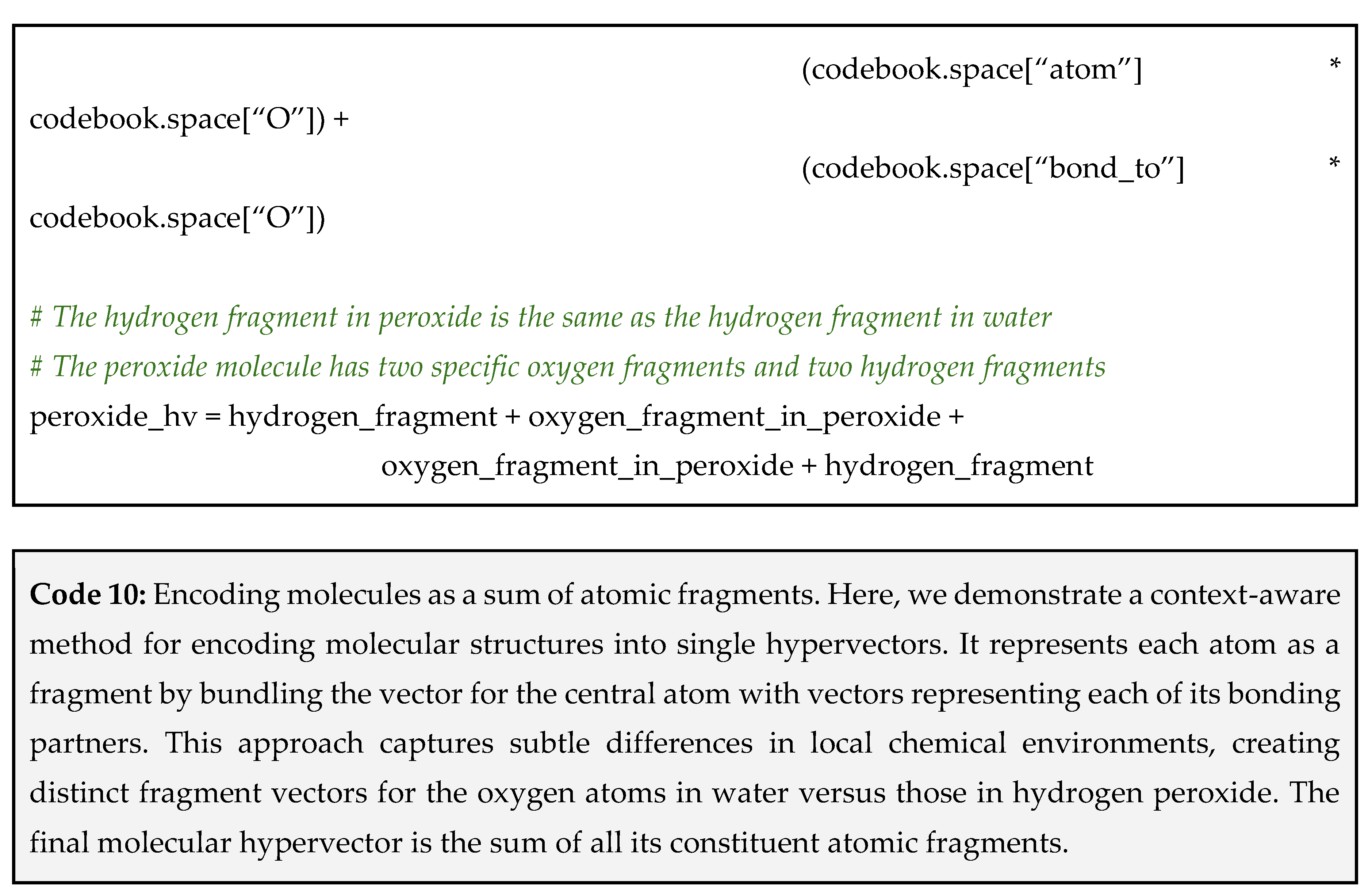
Why This Works
This compositional and context-aware approach allows the creation of highly descriptive vectors and the prediction of a molecule’s properties based on the similarity of its vector to known prototypes. Imagine we have built a prototype vector for soluble and insoluble compounds by averaging the vectors of many known examples.
To predict the solubility of a new molecule, we first construct its hypervector and then see which prototype it resembles more closely.
This method effectively translates the complex graph-based problem of cheminformatics into a vector-space similarity problem allowing for fast, scalable, and surprisingly accurate predictions of molecular properties.
Pitfall: ignore stereochemistry and 3D information – the refined fragment encoding is good, but it still represents the molecule as a 2D graph. It cannot distinguish between enantiomers (left- and right-handed versions of a molecule), which can have drastically different biological effects (e.g., Thalidomide).
How to avoid the pitfall: add 3D information to the codebook – enrich your fragments. In addition to bond_to, you can add vectors for stereochemical information like r_config or s_config at chiral centers. You can also discretize bond angles or dihedral angles and bind this information into the fragment vector to provide a richer, more 3D-aware representation. Practically, encoding left–right and numerical angle features in HDC is straightforward. For numerical angles, we can use correlation-aware codes so that nearby values are more similar while distant ones decorrelate. Since angles exist in a bounded range (0–360°), building an angle codebook is simple. During molecule construction, this requires only one additional binding step to inject the tag. Multi-stage cascading of such encodings (bond type, angle/dihedral, role) remains both simple and effective. One crucial point is that symbolic roles (left, right, top, bottom, etc.) should remain orthogonal and be drawn from independent random sources to ensure a clear distinction.
Tip 6: For Biomedical Knowledge Graphs – Use Binding to Represent Relational Triples
The biomedical field is flooded with massive databases containing information about which genes are associated with which diseases, what proteins interact with each other, which drugs inhibit certain enzymes, and many other relational information. These networks of relationships form a knowledge graph [49,50,51]. A key challenge is how to represent this graph in a way that allows us to reason with it, infer new relationships, and answer complex questions. Traditional graph databases can be rigid and computationally expensive to query for fuzzy or incomplete matches.
Facts as Vectors
VSAs provide a powerful way to encode an entire knowledge graph into a single, dense hypervector (or a collection of them). The fundamental unit of a knowledge graph is the relational triple <subject, predicate, object> (e.g., <caffeine, inhibits, adenosine_receptor>).
The VSA solution is to use the binding operation to compress this entire triple into a single hypervector. This fact vector represents the complete relationship. By bundling thousands of these fact vectors together, we can create a composite vector that represents a vast body of knowledge:
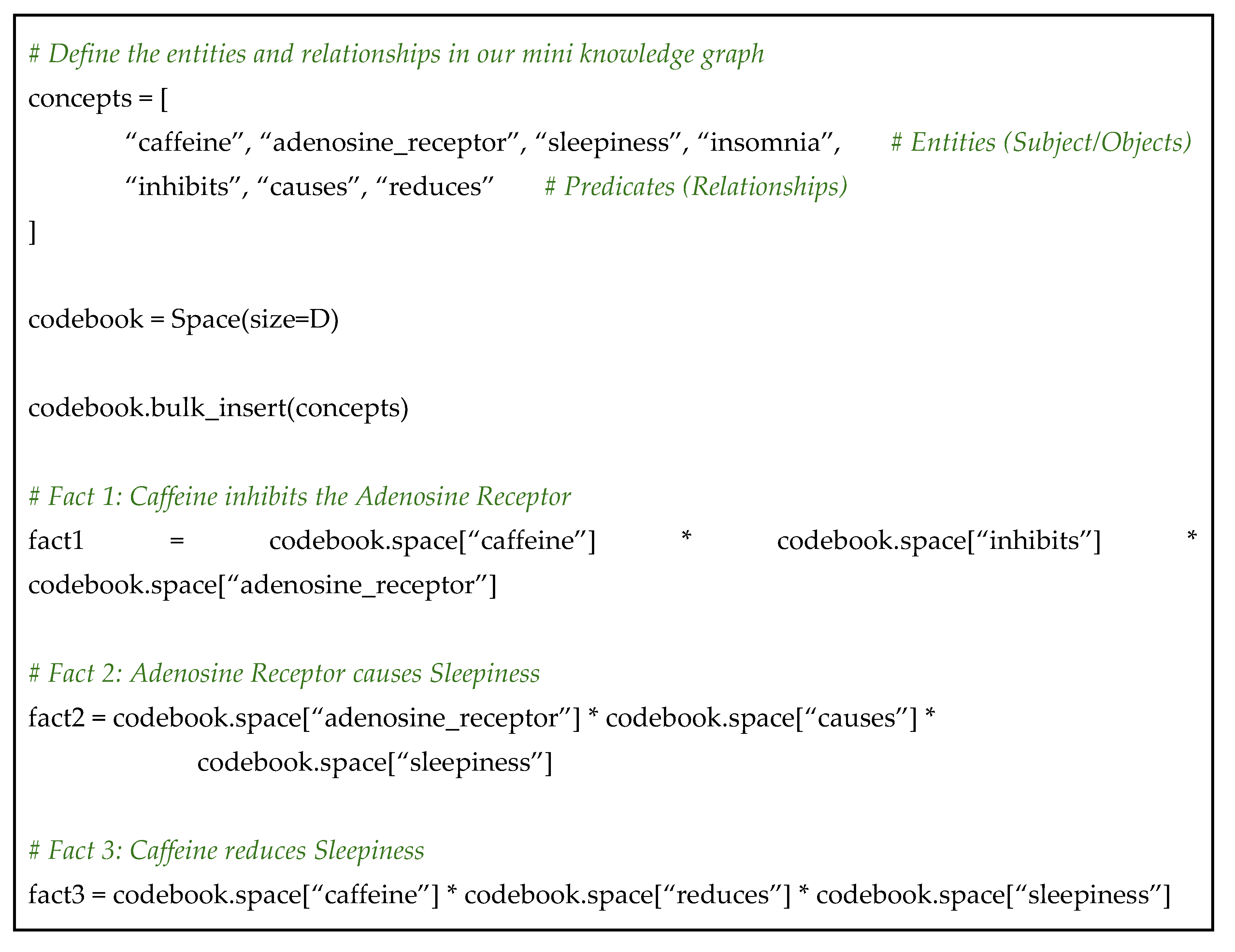
Step 1: building a codebook for entities and predicates – first, we create a dictionary that maps every entity (like a drug, gene, or disease) and every predicate (a relationship, like causes, inhibits, or interacts_with) to a unique hypervector;
Step 2: encode each fact using binding – now, for each triple in our knowledge graph, we create a fact vector by binding the subject, predicate, and object together;
Step 3: bundle facts into a knowledge base vector – to create our final knowledge base, we simply bundle all the individual fact vectors together. The single vector now contains all the information from our original graph, stored in a distributed, superimposed manner.
Code 11 summarizes the whole procedure.

Why This Works
The true power of this representation lies in its ability to answer questions and infer relationships through vector arithmetic. We can query the knowledge base by providing parts of a triple and using the inverse operation to find the missing piece.
Question: “What does caffeine inhibit?”
To answer this question, we create a query vector by binding caffeine and inhibits, and then bind this to our knowledge base along with the query vector as shown in Code 12.
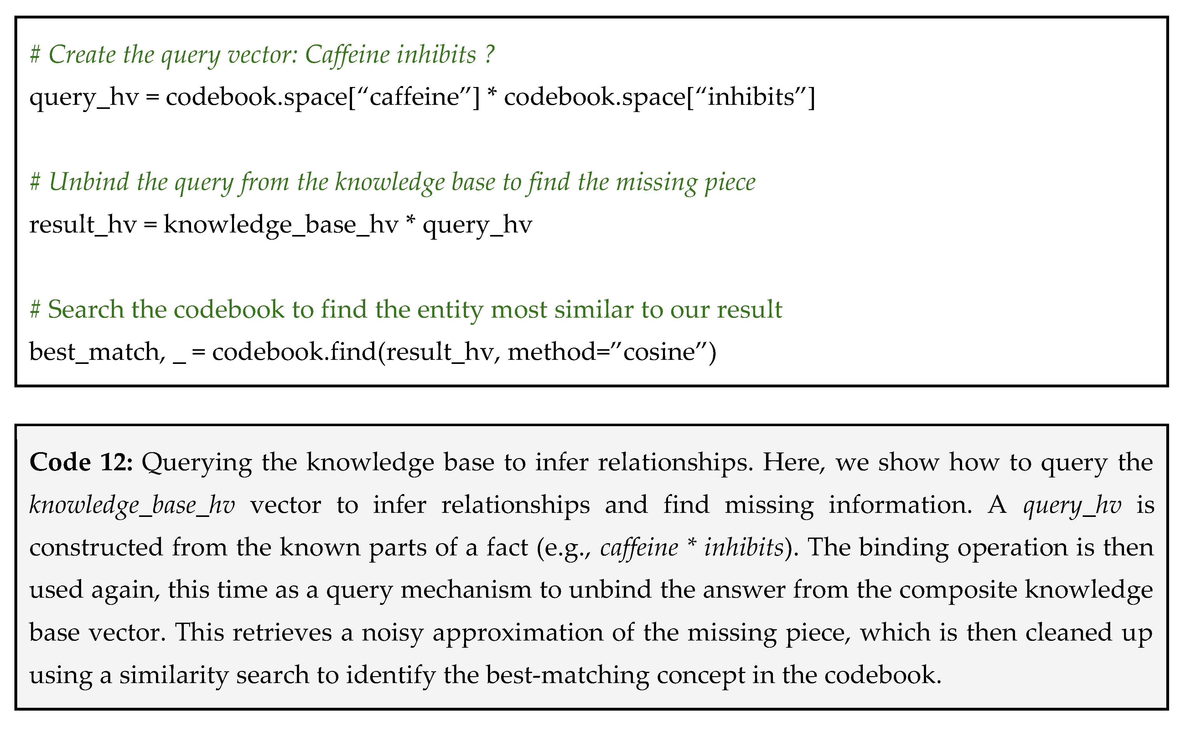
This VSA technique allows for powerful, fuzzy queries on massive datasets. It can be used to infer novel drug-repurposing candidates, discover potential gene-disease associations, and build systems that can reason over the vast and ever-growing body of biomedical literature.
Pitfall: ambiguity of the unbind operation – when you query the knowledge base, the result vector is an approximation, not a clean answer. It is a superposition of the correct answer plus noise from all other facts in the knowledge base. If your knowledge base is very dense with similar relationships, the noise can overwhelm the signal, and the top match for your query might be incorrect.
How to avoid the pitfall: use cleanup memory – after you get your result_hv, do not just find the single best match in your codebook. Instead, find the top 3-5 closest matches and bundle them together. Then, use this new, cleaner vector to re-query the codebook. This process, also called iterative cleanup, helps to amplify the signal and suppress the noise, leading to more accurate query results.
Tip 7: For Classification Tasks – Build and Refine Prototype Vectors
In many biomedical scenarios, collecting large, labeled datasets for training complex machine learning models is a difficult task. You might have detailed data for thousands of healthy individuals but only a few dozen patients with a rare disease. Training sophisticated models like deep neural networks on such imbalance or small datasets is often impractical and can lead to poor performance [52,53]. The challenge is to build a reliable classifier that can learn effectively from a small number of samples (a concept known as few-shot learning) [54,55,56].
Learning the Average Case
The VSA approach for classification is beautifully simple and effective. Instead of learning a complex decision boundary, we create a single prototype vector for each class. A prototype vector is simply the bundle of all the sample vectors belonging to that class. The learning process happens incrementally, with each sample contributing additively to the prototype hypervector. Thus, the reverse operation, unlearning, is simply subtracting that contribution.
Let’s consider an hypothetical prototype_diabetic vector that represents the central tendency of all diabetic patients in your training set. To classify a new patient, you simply check if their vector is more similar to the diabetic prototype or the non-diabetic prototype. This method is transparent, computationally cheap, and works remarkably well even with very few training samples.
Let’s assume we have already encoded our data into hypervectors. For this example, we will use the patient vectors created in Tip 1, where each vector represents a patient’s EHR data. Our goal is to classify patients as either diabetic or non_diabetic:
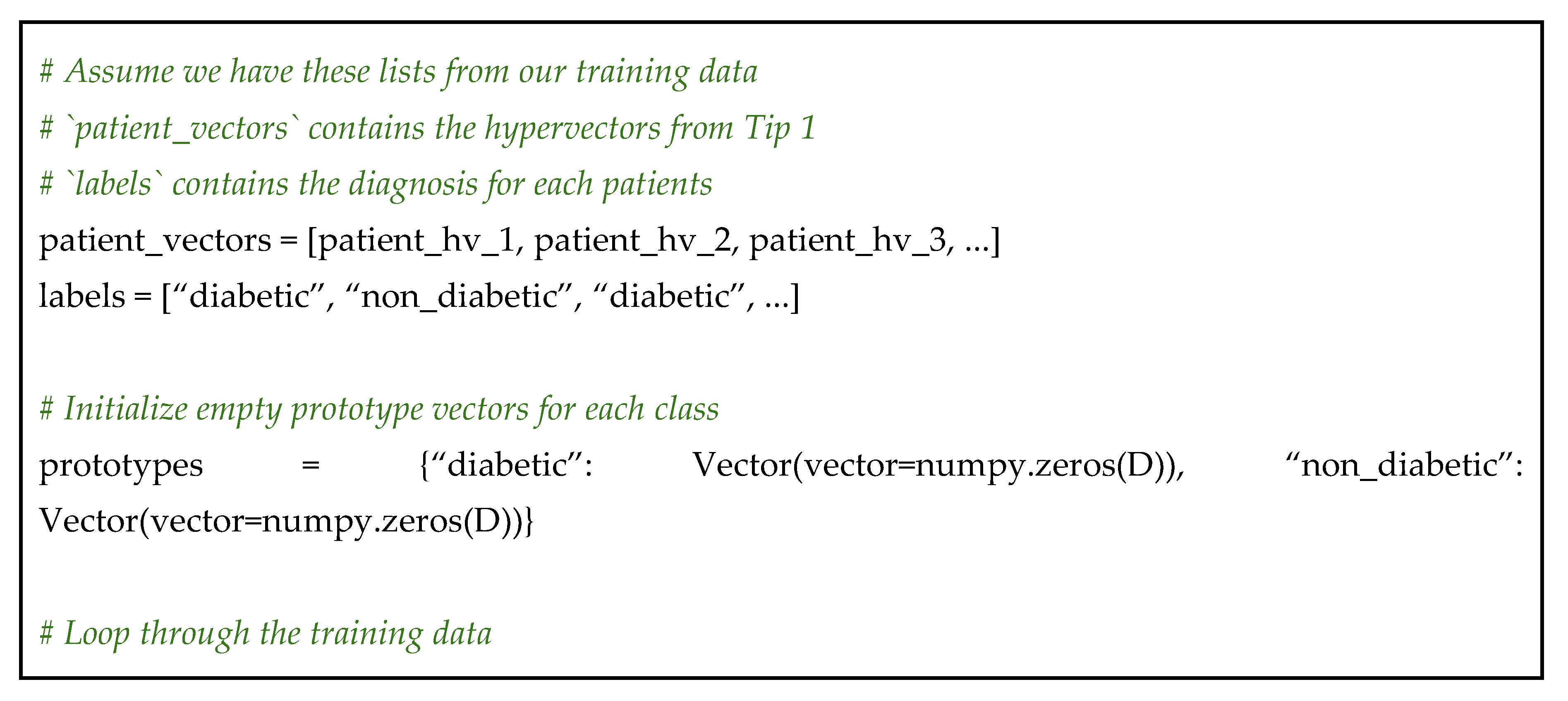
Step 1: encode your training data – first, ensure every sample in your labeled training set is represented as a hypervector. We will presuppose this step is complete and we have a list of patient vectors and their corresponding labels;
Step 2: create a prototype vector for each class – now, we iterate through our training data. We will add each patient’s vector to a running sum for their respective class;
Step 3: classify a new sample with similarity search – with our prototypes built, classification is incredibly straightforward. For any new, unlabeled patient vector, we calculate its cosine distance to each prototype vector. The class of the prototype with the lowest distance score is our predicted class (see Code 13 for a code overview).
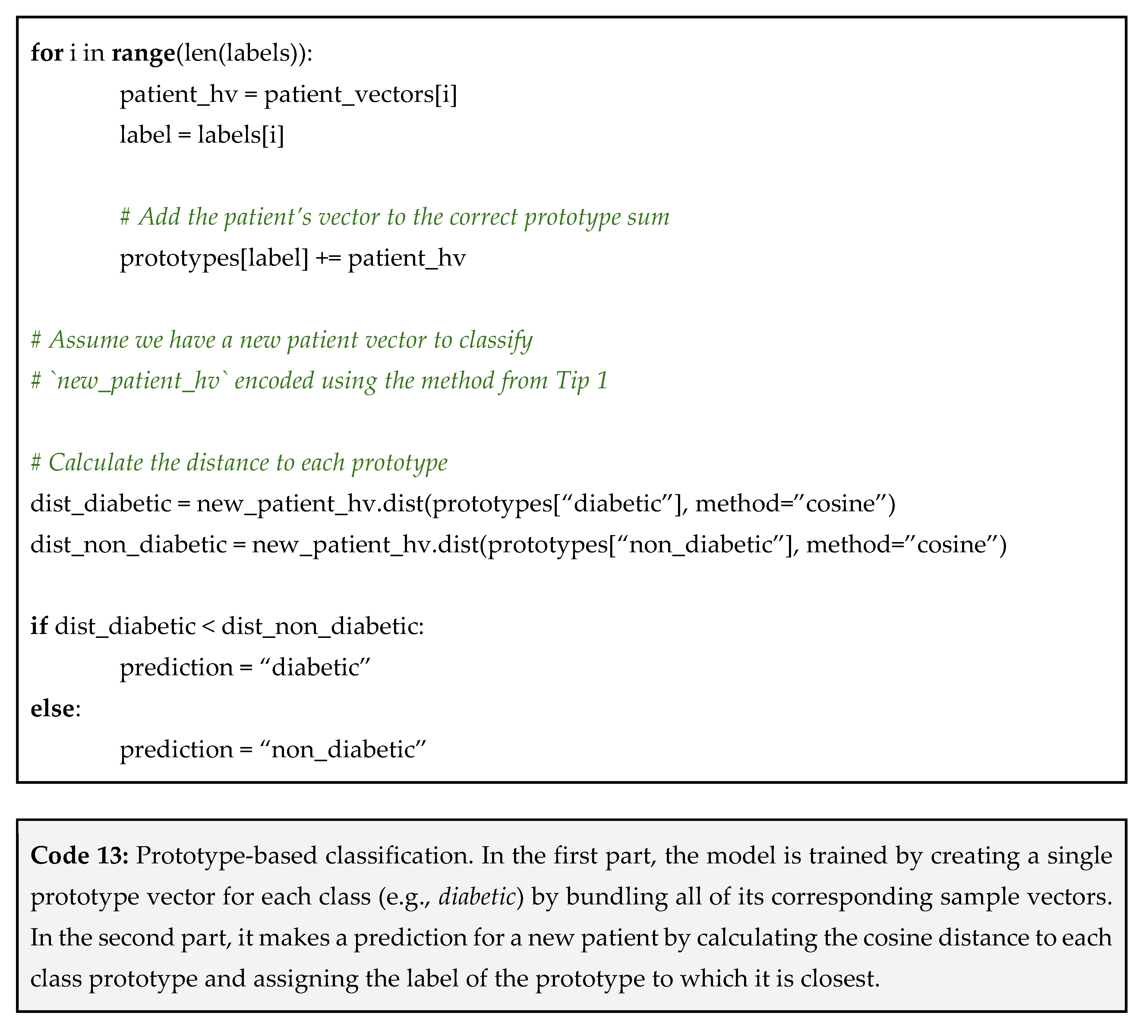
Why This Works
This prototype-based method is a cornerstone of applied VSA for several reasons:
- Simplicity and speed: the training phase is just one pass of addition. The prediction phase is just a few similarity calculations. This is orders of magnitude faster than training a deep neural network;
- Excellent for few-shot learning: this method creates a reasonable prototype even with just a few samples per class;
- Incremental learning/unlearning: if you get new labeled data, you do not have to retrain your model from scratch. You can simply update the existing prototype sums with the new vectors, allowing your model to learn continuously. Conversely, if data needs to be removed, the update is just a subtraction from the prototype.
Pitfall: class size imbalance dominates prototypes – if you create prototypes by summing vectors, the class with more samples will produce a prototype vector with a much larger magnitude. For example, if you have 1,000 healthy samples and only 50 rare_disease samples, the prototype_healthy vector will be mathematically dominant. Consequently, almost every new sample, even those with the disease, will be more similar to the stronger healthy prototype, making your classifier extremely biased toward the majority class.
How to avoid the pitfall: normalize the final prototype vectors – after you have finished summing all the vectors for each class, normalize the final prototype vectors so they all have the same magnitude. This crucial step removes the bias from class size imbalance. It ensures that a sample’s classification is based purely on the pattern of the prototype, not its magnitude (the number of samples used to create it).
Tip 8: For Data Fusion – Map All Modalities into a Common Vector Space
A single patient’s story is often told across multiple data types, or modalities. A clinician might have an MRI scan (an image), a radiologist’s report (text), genetic markers (sequential data), and basic lab results (numerical data). Each modality provides a piece of the puzzle, and the richest insights come from combining them [22,23,57]. The core challenge is that these data types are fundamentally incompatible. You cannot just add a pixel to a word or a gene to a blood pressure reading. How can you create a single, unified representation that respects the information from all sources?
A Universal Language
The elegance of VSAs is that hypervectors act as a universal language. As long as all your vectors share the same dimensionality, they can be mathematically combined, regardless of their origin. The strategy for data fusion is simple:
- Encode each modality separately into its own hypervector using the most appropriate technique (e.g., methods from Tip 1 for text/EHRs, Tip 2 for genetic sequences, Tip 3 for images);
- Bundle the resulting vectors together to create a single, multimodal hypervector that represents the complete picture.
This allows to create a holistic patient representation that is richer than any single data source alone. Let’s imagine our goal is to create a single patient vector that combines the findings from a written radiology report and the corresponding MRI scan:
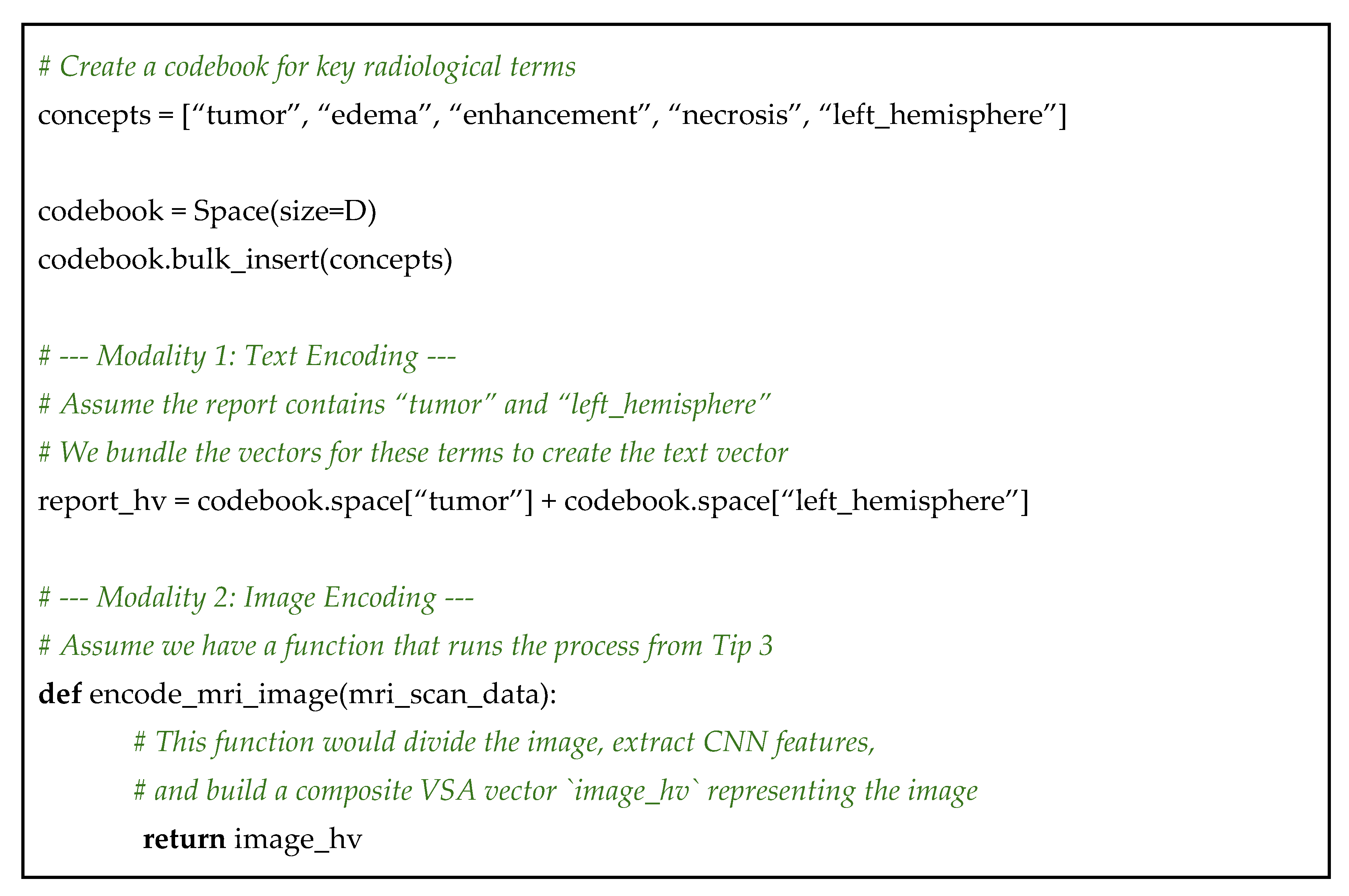
Step 1: encode the text modality – first, we process the text from the radiology report. We can use a method similar to Tip 1, creating a simple bag-of-words vector by bundling the vectors for key terms found in the report;
Step 2: encode the image modality – next, we process the MRI scan. As described in Tip 3, we would use a hybrid CNN-VSA approach to convert the image into a single hypervector. This image_hv symbolically represents the key features and their locations within the scan;
Step 3: bundle the modalities into a unified vector – this is the easiest and most powerful step. To create the final, multimodal representation of the patient’s case, we simply bundle the report_hv and the image_hv together.
This is all summarized in Code 14 below.
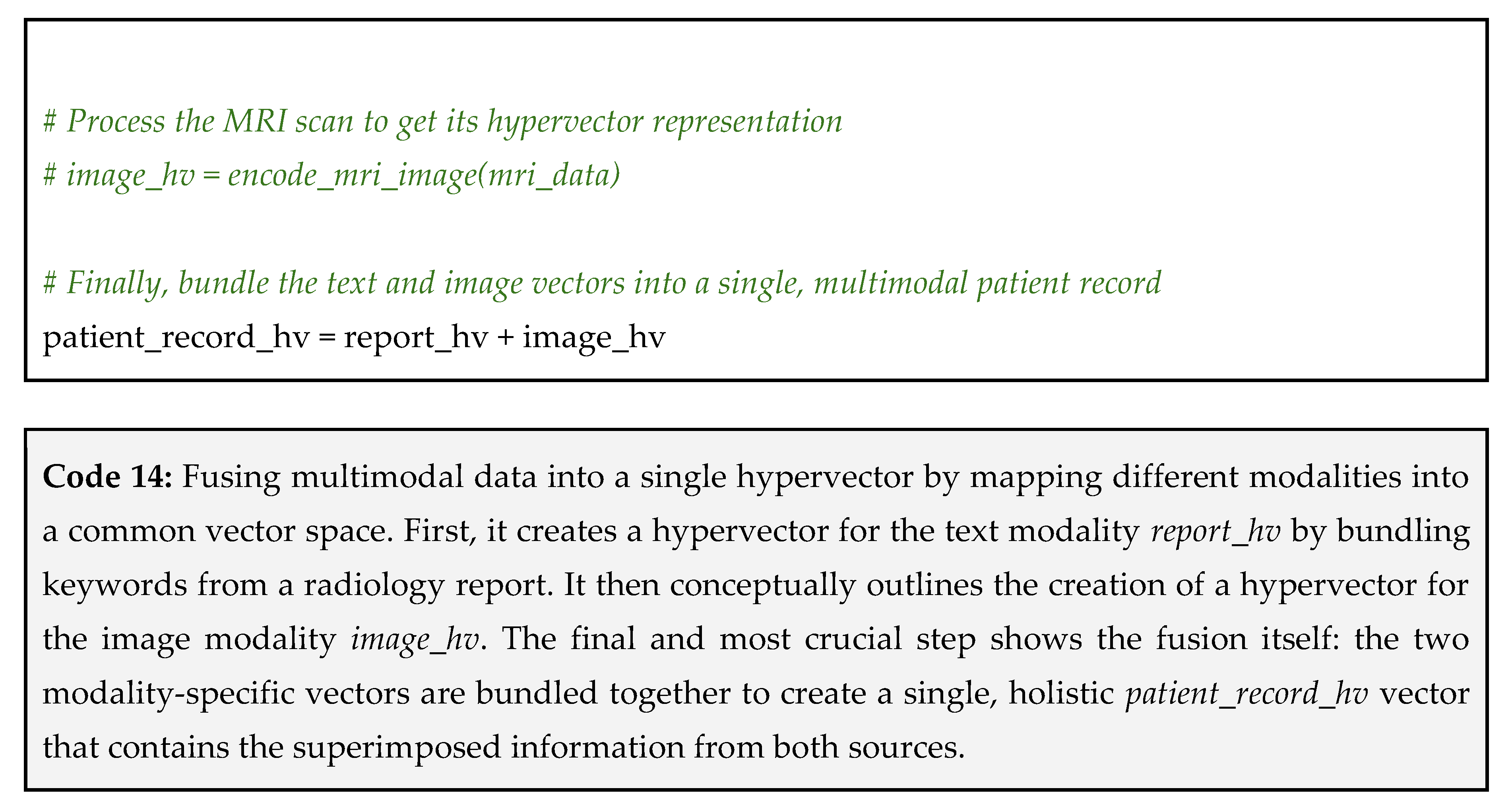
Why This Works
The resulting patient_record_hv from Code 14 is a single vector that contains superimposed information from both the text and the image. In our example, it contains tumor from both sources, left_hemisphere from the text, and edema from the image. This fused vector is a more complete and robust representation than either vector alone. When used for classification (Tip 7), this richer vector will lead to more accurate predictions because it can draw on evidence from multiple sources.
Pitfall: modality imbalance – if one modality is represented in a much more complex way than another, its vector might have a larger magnitude or simply contain more information, causing it to drown out the contribution of the other modality during bundling. For instance, a complex image vector might dominate a simple text vector derived from just two keywords.
How to avoid the pitfall: normalize each modality vector before bundling – before you add the vectors together, normalize each one individually. Normalization scales a vector to have a standard magnitude without changing its direction in the high-dimensional space. This ensures that each modality contributes its pattern to the final vector with equal strength, regardless of how many components were used to create it. An alternative is to binarize each incoming vector prior to bundling while preserving a balanced bipolar distribution. This resets the accumulation to binary values and prevents any one data type (e.g., scalar-heavy inputs) from dominating the superposed result.
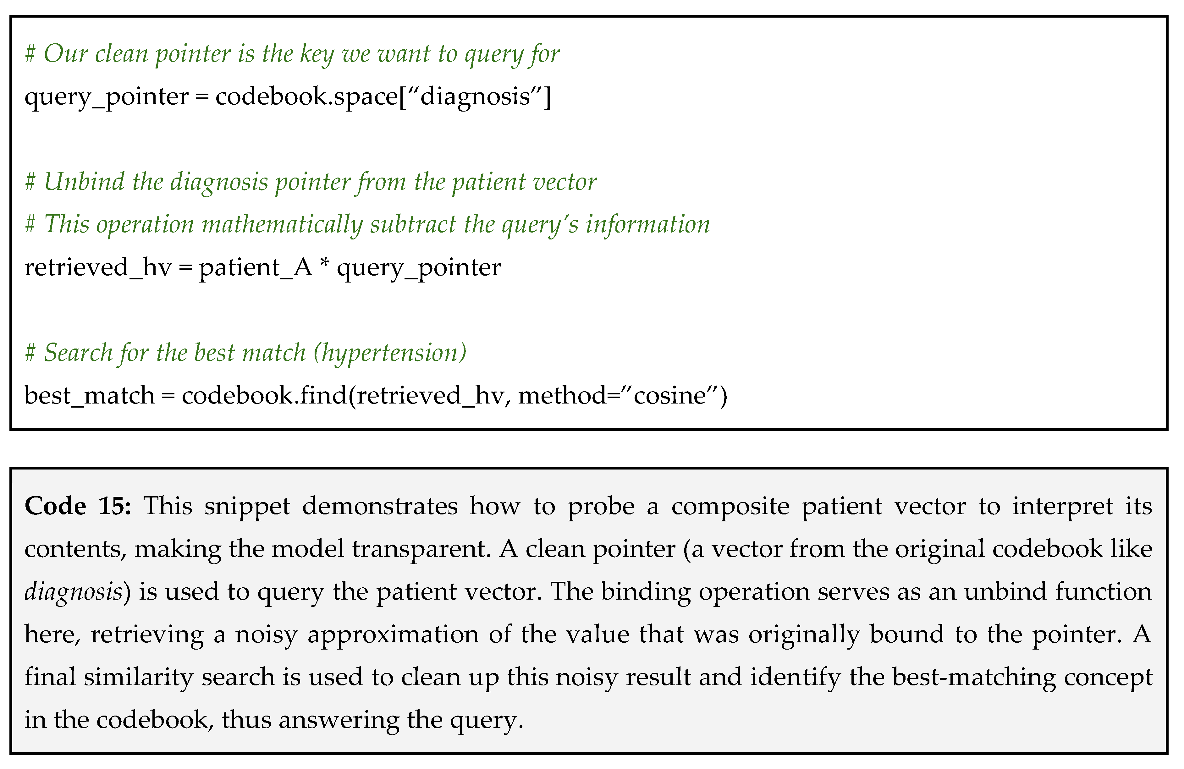
Tip 9: For Interpreting Results – Probe Composite Vectors with Clean Pointers
In Tip 1, we have built a model that takes a patient’s EHR data, encodes it into a single hypervector, and correctly classifies patients as having high risk for a certain disease. But now comes the critical question from the clinician: “Why?”. What specific information in that patient’s record led to this conclusion? With many machine learning models (the so-called black boxes), this question is nearly impossible to answer because of the model’s internal logic.
Asking Your Vector Questions
A composite hypervector is not a black box. It is a queryable database. Because it was constructed using symbolic components, you can reverse the process to inspect its contents. The technique involves using a clean pointer and the inverse of the binding operation to ask the composite vector a question. This process essentially asks “What information in you is associated with this pointer I am holding?”. This makes VSA models highly interpretable and transparent [58,59,60,61].
Let’s use the composite patient_A we created back in Tip 1. Recall that it was constructed from three facts: a diagnosis of hypertension, a prescription for metformin, and a high HbA1C lab result. Here is the question: “What was this patient’s diagnosis?”
Step 1: construct your query vector (the clean pointer) – your query is the part of the fact that you already know. In this case, we know the key is diagnosis;
Step 2: unbind the pointer from the composite vector – to retrieve the value associated with our pointer, we use the binding operation;
Step 3: find the closest match in your codebook – the resulting vector is not a perfect, clean vector. It is a noisy approximation of the answer because it also contains remnants of all other bundled information. To get our final answer, we search our codebook to find the vector that is most similar to the retrieved one (see Code 15 below).
Pitfall: noisy or ambiguous answers – when unbinding a pointer, the resulting vector is an approximation that is contaminated by noise from all the other bundled vectors. If your composite vector is extremely dense (contains hundreds of bundled facts), this noise can become so strong that the similarity to the correct answer is low, and the similarity to incorrect answers might be non-zero, creating ambiguity.
How to avoid the pitfall: use cleanup memory – the process of finding the closest match in the codebook is itself a form of cleanup. To make it more robust, you can perform an extra cleanup step. Instead of taking just the single best match, take the top 2-3 matches, bundle them together, and then search the codebook again with this new, denoised vector. For most applications, however, a direct search is sufficient. A better long-term solution is to design your encoding scheme hierarchically (as discussed in the solution proposed to avoid Tip 2 pitfall) to limit how many items get bundled into a single vector.
Tip 10: For Reproducibility and Impact – Practice Open Science
In computational fields, a research paper is only half of the story. A paper might describe a novel method and present compelling results, but if the underlying code and data are kept private, the work exists in a “silo” [62]. Other researchers cannot verify the findings, replicate the analysis on their own data, or build upon the method without reinventing it from scratch. This lack of transparency slows down scientific progress and can create a crisis in reproducibility, where it is impossible to know if a method truly works as described.
The best way to maximize the impact of and trustworthiness of your work is to practice Open Science, guided by the FAIR Guiding Principles [63]. The goal is to make your research outputs, including data, code, and models, Findable, Accessible, Interoperable, and Reusable. This framework moves beyond just making things public, and provides a clear roadmap for creating truly useful and lasting scientific contributions:
- Ensure others can easily discover your work: assign a Digital Object Identifier (DOI) to your code and data by using a repository like Zenodo or Figshare. This makes them easily citable. Also, use rich metadata and keywords when you upload your assets. Describe what the data contains, the VSA parameters used, and the context of the study;
- Make your research available to everyone: publish your code in a public repository like GitHub or GitLab. Submit your manuscript to a fully Open Access Journal to remove paywalls. The protocol for accessing the data should be open and free;
- Ensure your data and models can be combined with other tools and datasets: use common, standard file formats for your input data instead of proprietary formats. Clearly document your VSA parameters, especially the dimensionality and the vector type. This allows others to integrate your hypervectors with their own VSA-based tools;
- Enable others to effectively build upon your work: provide clear and comprehensive documentation. A README.md file in your code repository should explain what the project does and how to run the analysis, including listing all necessary software libraries and their version. Choose a permissive open-source license (e.g., MIT or Apache 2.0) that explicitly tells others how they are allowed to reuse your code.
Following the FAIR principles directly leads to more robust science. It enhances reproducibility, foster collaborations, increase the visibility and impact of your work, and builds trust within the scientific community. Currently, considering the recent VSA architecture open-source platforms, researchers can take advantage of libraries such as TorchHD [64], DistHD [65], OpenHD [66], HDTorch [67], uHD [68] and hdlib [11], the one mainly used for this work. Unlike some other frameworks that focus narrowly on GPU acceleration or domain-specific encodings, hdlib was designed from the start as a general-purpose library for building VSAs. hdlib offers a clean, modular structure for defining high-dimensional spaces and vectors, performing the canonical operations of bind, bundle, and permute, and supporting supervised learning with built-in cross-validation, auto-tuning, and even feature selection, making it a versatile framework.
Conclusions
VSAs provide a powerful and intuitive paradigm for tackling the complex, heterogeneous, and often incomplete data that characterizes the biomedical sciences. This work has moved beyond abstract theory and offers a set of practical, application-driven tips for researchers. We have demonstrated how the core VSA operations of binding, bundling, and permutation can be combined to solve diverse challenges.
We began by showing how to construct holistic representations from disparate data sources. For electronic health records, we demonstrated how bundling can create robust patient vectors that naturally handle missing information (Tip 1), while for molecular structures, we showed how to encode a molecule as a sum of its context-aware atomic fragments (Tip 5). The critical role of order was addressed for genomics and proteomics, where permutation is key to encoding sequences (Tip 2), and for biosignals like EEG, where symbolic snapshots can capture dynamic states over time (Tip 4).
We also illustrated how VSAs can be applied to high-level reasoning and data fusion tasks. We explored a method for building prototype vectors to create simple yet powerful classifiers (Tip 7) and showed how VSAs can represent vast biomedical knowledge graphs as queryable vectors (Tip 6). Furthermore, we detailed how VSAs can augment other computational methods, such as combining them with CNNs to build explainable models for medical imaging (Tip 3), and how they provide a universal language for the fusion of multimodal data into a single, unified representation (Tip 8).
A recurring theme throughout these tips is the shift from black box models to transparent systems. The ability to probe a composite hypervector to ask “why” (Tip 9) is a standout feature that addresses a key limitation of many conventional methods. Ultimately, the power of any computational method is magnified by the community that uses it. For this reason, we concluded with a crucial tip on practicing FAIR and Open Science (Tip 10). A well-designed model becomes truly transformative only when its code and derived data are shared openly, allowing for verification, replication, and extension by the entire scientific community.
As the scale and complexity of biomedical data continue to grow, brain-inspired approaches like HDC will be indispensable. By moving beyond pure pattern recognition towards models that can represent, reason with, and explain complex information, researchers are now better equipped to build the next generation of tools to unlock new insights from the full spectrum of biomedical data.
Author Contributions
FC conceived the research; FC designed and conceived the tips, implemented the code, and defined pitfalls; FC, DC, SA, and DB discussed the hyperdimensional computing framework and biomedical applications; FC, DC, SA, and DB wrote the manuscript and agreed with its final version.
Funding
The authors declare that no funding was received for the conception or writing of this manuscript.
Data Availability Statement
All source code required to reproduce the examples in this manuscript is open source and publicly available on GitHub at https://github.com/cumbof/Biomed-VSAs. The repository contains a series of self-contained Jupyter notebooks that provide a runnable implementation for each technical tip discussed. The same code is also archived on Zenodo at https://doi.org/10.5281/zenodo.17107789.
Acknowledgments
The authors acknowledge the use of AI-powered language tools to enhance the clarity and readability of this manuscript. The AI’s role was strictly limited to improving prose and sentence structure. The conceptual framework of this manuscript, the formulation of tips, the design of the code examples, and all scientific recommendations were developed exclusively by the authors.
Conflicts of Interest
FC and DC are Academic Editors for PeerJ Computer Science.
Abbreviations
| AI | Artificial Intelligence |
| CNN | Convolutional Neural Network |
| DOI | Digital Object Identifier |
| ECG | Electrocardiography |
| EEG | Electroencephalography |
| EHR | Electronic Health Record |
| EMG | Electromyography |
| FAIR | Findability, Accessibility, Interoperability, and Reusability |
| HDC | Hyperdimensional Computing |
| MAP | Multiply-Add-Permute |
| MRI | Magnetic Resonance Imaging |
| VSA | Vector-Symbolic Architecture |
References
- Kanerva, P. Hyperdimensional computing: An introduction to computing in distributed representation with high-dimensional random vectors. Cognit Comput. 2009, 1, 139–159. [Google Scholar] [CrossRef]
- Kanerva, P. Hyperdimensional computing: An algebra for computing with vectors. Advances in Semiconductor Technologies. Wiley; 2022. pp. 25–42. [CrossRef]
- Zhang S, Wang R, Zhang JJ, Rahimi A, Jiao X. Assessing robustness of hyperdimensional computing against errors in associative memory : (invited paper). 2021 IEEE 32nd International Conference on Application-specific Systems, Architectures and Processors (ASAP). IEEE; 2021. [CrossRef]
- Zhang S, Juretus K, Jiao X. Exploring hyperdimensional computing robustness against hardware errors. IEEE Trans Comput. 2025, 74, 1963–1977. [Google Scholar] [CrossRef]
- Burrello A, Schindler K, Benini L, Rahimi A. Hyperdimensional Computing With Local Binary Patterns: One-Shot Learning of Seizure Onset and Identification of Ictogenic Brain Regions Using Short-Time iEEG Recordings. IEEE Trans Biomed Eng. 2020, 67, 601–613. [Google Scholar] [CrossRef]
- Burrello A, Schindler K, Benini L, Rahimi A. One-shot learning for iEEG seizure detection using end-to-end binary operations: Local binary patterns with hyperdimensional computing. 2018 IEEE Biomedical Circuits and Systems Conference (BioCAS). IEEE; 2018. [CrossRef]
- Rahimi A, Tchouprina A, Kanerva P, Millán J del R, Rabaey JM. Hyperdimensional Computing for Blind and One-Shot Classification of EEG Error-Related Potentials. Mobile Networks and Applications. 2017, 25, 1958–1969. [Google Scholar] [CrossRef]
- Nair DR, Purushothaman A. Brain Inspired One Shot Learning Method for HD Computing. VLSI Design and Test. 2019, 286–297. [Google Scholar] [CrossRef]
- Cumbo F, Chicco D. Hyperdimensional computing in biomedical sciences: a brief review. PeerJ Comput Sci. 2025, 11, e2885. [Google Scholar] [CrossRef]
- Stock M, Van Criekinge W, Boeckaerts D, Taelman S, Van Haeverbeke M, Dewulf P, et al. Hyperdimensional computing: A fast, robust, and interpretable paradigm for biological data. PLOS Computational Biology. 2024, 20, e1012426. [Google Scholar] [CrossRef]
- Cumbo F, Weitschek E, Blankenberg D. hdlib: A Python library for designing Vector-Symbolic Architectures. J Open Source Softw. 2023, 8, 5704. [Google Scholar] [CrossRef]
- Sæthre E, Osborg Ose S, Krokstad S, Østgård Gismervik S. “Terrible Stuff. We’ve been had“: hospital staff reactions to a new electronic health record and implications for employee well-being – A qualitative study. International Journal of Medical Informatics. 2025, 204, 106039. [Google Scholar] [CrossRef]
- Tavabi N, Singh M, Pruneski J, Kiapour AM. Systematic evaluation of common natural language processing techniques to codify clinical notes. PLoS One. 2024, 19, e0298892. [Google Scholar] [CrossRef]
- Sheikhalishahi S, Miotto R, Dudley JT, Lavelli A, Rinaldi F, Osmani V. Natural Language Processing of Clinical Notes on Chronic Diseases: Systematic Review. JMIR Med Inform. 2019, 7, e12239. [Google Scholar] [CrossRef]
- Kuo T-T, Rao P, Maehara C, Doan S, Chaparro JD, Day ME, et al. Ensembles of NLP Tools for Data Element Extraction from Clinical Notes. AMIA Annu Symp Proc. 2016, 2016, 1880–1889. [Google Scholar]
- Wells BJ, Chagin KM, Nowacki AS, Kattan MW. Strategies for handling missing data in electronic health record derived data. EGEMS (Wash DC). 2013, 1, 1035. [Google Scholar] [CrossRef]
- Jones JA, Farnell B. Missing and Incomplete Data Reduces the Value of General Practice Electronic Medical Records as Data Sources in Research. Aust J Prim Health. 2007, 13, 74–80. [Google Scholar] [CrossRef]
- Joel LO, Doorsamy W, Paul BS. A Review of Missing Data Handling Techniques for Machine Learning. IJITIS. 2022, 5, 971–1005. [Google Scholar] [CrossRef]
- Emmanuel T, Maupong T, Mpoeleng D, Semong T, Mphago B, Tabona O. A survey on missing data in machine learning. Journal of Big Data. 2021, 8, 1–37. [Google Scholar] [CrossRef]
- Rizvi STH, Latif MY, Amin MS, Telmoudi AJ, Shah NA. Analysis of Machine Learning Based Imputation of Missing Data. Cybernetics and Systems. 2023, 818–832. [Google Scholar] [CrossRef]
- Bai T, Chanda AK, Egleston BL, Vucetic S. EHR phenotyping via jointly embedding medical concepts and words into a unified vector space. BMC Medical Informatics and Decision Making. 2018, 18, 15–25. [Google Scholar] [CrossRef]
- Chang E-J, Rahimi A, Benini L, Wu A-YA. Hyperdimensional computing-based multimodality emotion recognition with physiological signals. 2019 IEEE International Conference on Artificial Intelligence Circuits and Systems (AICAS). IEEE; 2019. [CrossRef]
- Zhao Q, Yu X, Hu S, Rosing T. MultimodalHD: Federated learning over heterogeneous sensor modalities using hyperdimensional computing. 2024 Design, Automation & Test in Europe Conference & Exhibition (DATE). IEEE; 2024. pp. 1–6. [CrossRef]
- Fanizzi N, d’Amato C. The blessing of dimensionality. Neurosymbolic Artificial Intelligence. 2025. [Google Scholar] [CrossRef]
- Imani M, Nassar T, Rahimi A, Rosing T. HDNA: Energy-efficient DNA sequencing using hyperdimensional computing. 2018 IEEE EMBS International Conference on Biomedical & Health Informatics (BHI). IEEE; 2018. [CrossRef]
- Zou Z, Chen H, Poduval P, Kim Y, Imani M, Sadredini E, et al. BioHD. Proceedings of the 49th Annual International Symposium on Computer Architecture. New York, NY, USA: ACM; 2022. [CrossRef]
- Xu W, Hsu P-K, Moshiri N, Yu S, Rosing T. HyperGen: compact and efficient genome sketching using hyperdimensional vectors. Bioinformatics. 2024, 40, btae452. [Google Scholar] [CrossRef]
- Salehi AW, Khan S, Gupta G, Alabduallah BI, Almjally A, Alsolai H, et al. A Study of CNN and Transfer Learning in Medical Imaging: Advantages, Challenges, Future Scope. Sustainability. 2023, 15, 5930. [Google Scholar] [CrossRef]
- Yao W, Bai J, Liao W, Chen Y, Liu M, Xie Y. From CNN to Transformer: A Review of Medical Image Segmentation Models. Journal of Imaging Informatics in Medicine. 2024, 37, 1529–1547. [Google Scholar] [CrossRef]
- Li Q, Cai W, Wang X, Zhou Y, Feng DD, Chen M. Medical image classification with convolutional neural network. 2014 13th International Conference on Control Automation Robotics & Vision (ICARCV). IEEE; 2014. [CrossRef]
- Xie Y, Zhang J, Shen C, Xia Y. CoTr: Efficiently Bridging CNN and Transformer for 3D Medical Image Segmentation. Medical Image Computing and Computer Assisted Intervention – MICCAI 2021. 2021; 171–180. [CrossRef]
- Yuan F, Zhang Z, Fang Z. An effective CNN and Transformer complementary network for medical image segmentation. Pattern Recognition. 2023, 136, 109228. [Google Scholar] [CrossRef]
- Hassan E, Halawani Y, Mohammad B, Saleh H. Hyper-dimensional computing challenges and opportunities for AI applications. IEEE Access. 2022, 10, 97651–97664. [Google Scholar] [CrossRef]
- Luczak P, Slot K, Kucharski J. Combining deep convolutional feature extraction with hyperdimensional computing for visual object recognition. 2022 International Joint Conference on Neural Networks (IJCNN). IEEE; 2022. pp. 1–8. [CrossRef]
- Lee H, Kim J, Chen H, Zeira A, Srinivasa N, Imani M, et al. Comprehensive integration of hyperdimensional computing with deep learning towards neuro-symbolic AI. 2023 60th ACM/IEEE Design Automation Conference (DAC). IEEE; 2023. pp. 1–6. [CrossRef]
- Alotaiby TN, Alshebeili SA, Alshawi T, Ahmad I, Abd El-Samie FE. EEG seizure detection and prediction algorithms: a survey. EURASIP Journal on Advances in Signal Processing. 2014, 2014, 1–21. [Google Scholar] [CrossRef]
- Ein Shoka AA, Dessouky MM, El-Sayed A, Hemdan EE-D. EEG seizure detection: concepts, techniques, challenges, and future trends. Multimedia Tools and Applications. 2023, 82, 42021–42051. [Google Scholar] [CrossRef] [PubMed]
- Rizal A, Priharti W, Hadiyoso S. Seizure detection in epileptic EEG using Short-Time Fourier Transform and support vector machine. Int J Onl Eng. 2021, 17, 65–78. [Google Scholar] [CrossRef]
- Pale U, Teijeiro T, Atienza D. Systematic Assessment of Hyperdimensional Computing for Epileptic Seizure Detection. Annu Int Conf IEEE Eng Med Biol Soc. 2021, 2021, 6361–6367. [Google Scholar] [CrossRef]
- Ge L, Parhi KK. Applicability of hyperdimensional computing to seizure detection. IEEE Open J Circuits Syst. 2022, 3, 59–71. [Google Scholar] [CrossRef]
- Schindler KA, Rahimi A. A Primer on Hyperdimensional Computing for iEEG Seizure Detection. Front Neurol. 2021, 12, 701791. [Google Scholar] [CrossRef]
- Asgarinejad F, Thomas A, Rosing T. Detection of Epileptic Seizures from Surface EEG Using Hyperdimensional Computing. Annu Int Conf IEEE Eng Med Biol Soc. 2020, 2020, 536–540. [Google Scholar] [CrossRef]
- Du Y, Ren Y, Wong N, Ngai ECH. Hyperdimensional computing with multiscale local binary patterns for scalp EEG-based epileptic seizure detection. IEEE Internet Things J. 2024, 11, 26046–26061. [Google Scholar] [CrossRef]
- Virtanen P, Gommers R, Oliphant TE, Haberland M, Reddy T, Cournapeau D, et al. SciPy 1.0: fundamental algorithms for scientific computing in Python. Nat Methods. 2020, 17, 261–272. [Google Scholar] [CrossRef]
- Gramfort A, Luessi M, Larson E, Engemann DA, Strohmeier D, Brodbeck C, et al. MEG and EEG data analysis with MNE-Python. Front Neurosci. 2013, 7, 267. [Google Scholar] [CrossRef]
- Ma D, Thapa R, Jiao X. MoleHD: Efficient drug discovery using brain inspired hyperdimensional computing. 2022 IEEE International Conference on Bioinformatics and Biomedicine (BIBM). IEEE; 2022. [CrossRef]
- Jones D, Zhang X, Bennion BJ, Pinge S, Xu W, Kang J, et al. HDBind: encoding of molecular structure with hyperdimensional binary representations. Scientific Reports. 2024, 14, 1–16. [Google Scholar] [CrossRef]
- Cumbo F, Dhillon K, Joshi J, Raubenolt B, Chicco D, Aygun S, et al. Predicting the toxicity of chemical compounds via Hyperdimensional Computing. bioRxiv. 2025. [Google Scholar] [CrossRef]
- Nicholson DN, Greene CS. Constructing knowledge graphs and their biomedical applications. Computational and Structural Biotechnology Journal. 2020, 18, 1414–1428. [Google Scholar] [CrossRef] [PubMed]
- Bonner S, Barrett IP, Ye C, Swiers R, Engkvist O, Bender A, et al. A review of biomedical datasets relating to drug discovery: a knowledge graph perspective. Brief Bioinform. 2022, 23. [Google Scholar] [CrossRef]
- Harnoune A, Rhanoui M, Mikram M, Yousfi S, Elkaimbillah Z, El Asri B. BERT based clinical knowledge extraction for biomedical knowledge graph construction and analysis. Computer Methods and Programs in Biomedicine Update. 2021, 1, 100042. [Google Scholar] [CrossRef]
- Bugnon LA, Yones C, Milone DH, Stegmayer G. Deep Neural Architectures for Highly Imbalanced Data in Bioinformatics. IEEE Trans Neural Netw Learn Syst. 2020, 31, 2857–2867. [Google Scholar] [CrossRef]
- Pes, B. Learning from high-dimensional biomedical datasets: The issue of class imbalance. IEEE Access. 2020, 8, 13527–13540. [Google Scholar] [CrossRef]
- Cumbo F, Cappelli E, Weitschek E. A Brain-Inspired Hyperdimensional Computing Approach for Classifying Massive DNA Methylation Data of Cancer. Algorithms. 2020, 13, 233. [Google Scholar] [CrossRef]
- Cumbo F, Truglia S, Weitschek E, Blankenberg D. Feature selection with vector-symbolic architectures: a case study on microbial profiles of shotgun metagenomic samples of colorectal cancer. Brief Bioinform. 2025, 26, bbaf177. [Google Scholar] [CrossRef]
- Cumbo F, Dhillon K, Joshi J, Chicco D, Aygun S, Blankenberg D. A novel Vector-Symbolic Architecture for graph encoding and its application to viral pangenome-based species classification. bioRxiv. 2025. [CrossRef]
- Chicco D, Cumbo F, Angione C. Ten quick tips for avoiding pitfalls in multi-omics data integration analyses. PLoS Comput Biol. 2023, 19, e1011224. [Google Scholar] [CrossRef]
- Barkam HE, Yun S, Chen H, Gensler P, Mema A, Ding A, et al. Reliable hyperdimensional reasoning on unreliable emerging technologies. 2023 IEEE/ACM International Conference on Computer Aided Design (ICCAD). IEEE; 2023. [CrossRef]
- Mitrokhin A, Sutor P, Summers-Stay D, Fermüller C, Aloimonos Y. Symbolic Representation and Learning With Hyperdimensional Computing. Front Robot AI. 2020, 7, 535245. [Google Scholar] [CrossRef]
- Chang C-Y, Chuang Y-C, Huang C-T, Wu A-Y. Recent progress and development of hyperdimensional computing (HDC) for edge intelligence. IEEE J Emerg Sel Top Circuits Syst. 2023, 13, 119–136. [Google Scholar] [CrossRef]
- Amrouch H, Imani M, Jiao X, Aloimonos Y, Fermuller C, Yuan D, et al. Brain-inspired hyperdimensional computing for ultra-efficient edge AI. 2022 International Conference on Hardware/Software Codesign and System Synthesis (CODES+ISSS). IEEE; 2022. [CrossRef]
- Sim, I. Data Sharing and Reuse. Principles and Practice of Clinical Trials. 2022, 2137–2158. [Google Scholar] [CrossRef]
- Wilkinson MD, Dumontier M, Aalbersberg IJ, Appleton G, Axton M, Baak A, et al. The FAIR Guiding Principles for scientific data management and stewardship. Scientific Data. 2016, 3, 1–9. [Google Scholar] [CrossRef]
- Heddes M, Nunes I, Vergés P, Kleyko D, Abraham D, Givargis T, et al. Torchhd: An Open Source Python Library to Support Research on Hyperdimensional Computing and Vector Symbolic Architectures. Journal of Machine Learning Research. 2023, 24, 1–10. [Google Scholar]
- Wang J, Huang S, Imani M. DistHD: A learner-aware dynamic encoding method for hyperdimensional classification. 2023 60th ACM/IEEE Design Automation Conference (DAC). IEEE; 2023. pp. 1–6. [CrossRef]
- Kang J, Khaleghi B, Rosing T, Kim Y. OpenHD: A GPU-Powered Framework for Hyperdimensional Computing. IEEE Trans Comput. 2022, 71, 2753–2765. [Google Scholar] [CrossRef]
- Simon WA, Pale U, Teijeiro T, Atienza D. HDTorch: Accelerating Hyperdimensional Computing with GP-GPUs for Design Space Exploration. ICCAD ’22: Proceedings of the 41st IEEE/ACM International Conference on Computer-Aided Design. [CrossRef]
- Aygun S, Moghadam MS, Najafi MH. UHD: Unary processing for lightweight and dynamic hyperdimensional computing. 2024 Design, Automation & Test in Europe Conference & Exhibition (DATE). IEEE; 2024. pp. 1–6. [CrossRef]
Figure 1.
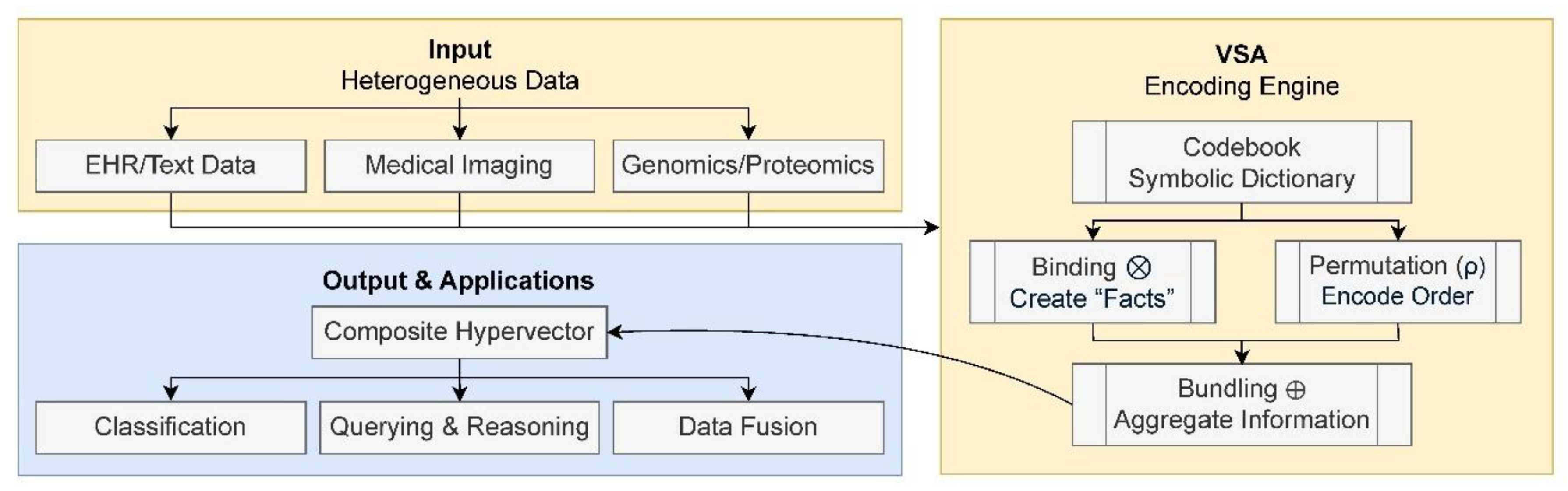
This flowchart illustrates the VSA process described here. Diverse biomedical data types (input) are first converted into symbolic hypervectors using a codebook and core operations like binding (for facts) and permutation (for sequences). This information is aggregated via bundling into a single, composite hypervector (output). This unified representation can then be used for various downstream tasks like classification, data fusion, and interpretable querying.
Figure 1.
This flowchart illustrates the VSA process described here. Diverse biomedical data types (input) are first converted into symbolic hypervectors using a codebook and core operations like binding (for facts) and permutation (for sequences). This information is aggregated via bundling into a single, composite hypervector (output). This unified representation can then be used for various downstream tasks like classification, data fusion, and interpretable querying.
Disclaimer/Publisher’s Note: The statements, opinions and data contained in all publications are solely those of the individual author(s) and contributor(s) and not of MDPI and/or the editor(s). MDPI and/or the editor(s) disclaim responsibility for any injury to people or property resulting from any ideas, methods, instructions or products referred to in the content. |
© 2025 by the authors. Licensee MDPI, Basel, Switzerland. This article is an open access article distributed under the terms and conditions of the Creative Commons Attribution (CC BY) license (http://creativecommons.org/licenses/by/4.0/).
Copyright: This open access article is published under a Creative Commons CC BY 4.0 license, which permit the free download, distribution, and reuse, provided that the author and preprint are cited in any reuse.


