Submitted:
01 October 2025
Posted:
01 October 2025
You are already at the latest version
Abstract
With the rapid growth of smart devices and positioning technologies, spatiotemporal data has become essential for predicting user behavior. However, many existing next-location prediction models employ oversimplified temporal modeling, neglect spatial structure and semantic relationships, and fail to capture complex location interaction patterns. This study proposes a graph neural network model that integrates spatiotemporal features to enhance next-location prediction. There are three components in the proposed method, the first is location feature representation which combines geocodes and location category embeddings to construct semantically enriched node representations. The second is temporal modeling which computes temporal similarity between historical trajectories and current behaviors to generate time-decay weights, thereby capturing behavioral periodicity and preference shifts. The third is preference integration which long-term historical preferences and short-term current preferences are modeled using a long short-term memory (LSTM) network and subsequently fused with spatial preferences to generate a comprehensive semantic representation encompassing both user preferences and location characteristics. Experiments on real-world trajectory datasets demonstrate that our proposed model achieves superior accuracy compared to state-of-the-art approaches in next-location prediction.
Keywords:
next-location prediction
; trajectory
; graph neural network
Introduction
In the task of predicting a user’s next location, one of the key challenges lies in effectively integrating the spatial characteristics of locations with the temporal patterns of user behavior to improve prediction accuracy. To address this challenge, recent research has emphasized training models on the trajectory data of all users, thereby capturing global behavioral patterns and spatiotemporal preferences. Leveraging these learned patterns, the model can infer the most probable next location for a user based on their recent trajectory, regardless of whether the user is new or existing.
The related definitions for predicting a user’s next location are as follows:
Let the user set be denoted as , where each user u has an associated trajectory record. The location set is defined as , where each location represents an encoded place. For example, A12 may indicate a specific convenience store (e.g., FamilyMart Guishan Branch), B07 may indicate a specific library (e.g., Taoyuan Library or Guishan Library), and C10 may indicate a specific restaurant (e.g., McDonald’s or KFC). Furthermore, let the location category set be defined as . Each location has a corresponding category , which denotes its categorical attribute. For instance, McDonald’s and KFC correspond to the “restaurant” category, FamilyMart and 7-Eleven correspond to the “convenience store” category, while Taoyuan Library and Guishan Library correspond to the “library” category.
Subsequently, a user’s trajectory data S is defined as a location sequence segmented by day, denoted as , in which represents the sequence of locations visited on the i-th day in chronological order. Each trajectory can also be mapped to a corresponding location category sequence , Furthermore, this study divides trajectories into two parts: the historical trajectory sequence and the current trajectory sequence .The prediction target is defined as the next potential location to be visited. In other words, given the historical trajectory and the current trajectory, the objective is to predict the location that the user is most likely to visit next.
In other words, the research problem can be described as follows: after collecting all users’ historical and current trajectory data (including location coordinates, location categories, and temporal information), how can we construct a predictive model that effectively learns group behavior patterns, and then, for any given user—whether a new user or one with existing records—infer the most likely next location based on their recent behavior. For example, if during the training phase the model observes that most users tend to visit a particular shopping district for lunch around noon, then when a user’s current trajectory indicates movement toward that area, the model should be able to predict, based on spatiotemporal behavioral features, that the user’s next step is likely to be visiting a restaurant in that district. This not only reflects current behavioral trends but also enables personalized recommendations aligned with individual preferences.
The aforementioned research problem highlights that modeling and integrating spatial and temporal information is one of the key challenges in predicting users’ next locations. In particular, locations not only contain geographic coordinates but also semantic categorical features, while users’ behavioral patterns are often influenced by temporal cycles and individual preferences. These complex factors must be effectively incorporated into predictive models. To design a system that truly reflects real-world user behavior, it is essential to explore how to process and represent these high-dimensional and dynamic spatiotemporal features. Based on this perspective, this study further elaborates its research motivation and objectives, examines the limitations of existing methods, and outlines the proposed model’s improvements and expected benefits.
In recent years, features such as geographic location, timestamps, and user behavior patterns have been widely utilized as crucial information for predicting users’ future movements in industries including tourism, smart cities, transportation management, and any domain where users’ dynamics can be observed through spatial and temporal data. Among these approaches, representing locations as embedding vectors has emerged as a particularly popular and innovative data processing method. Embedding vectors refer to techniques that transform high-dimensional sparse data (e.g., text, locations, images) into low-dimensional dense representations [4]. In machine learning, embeddings are commonly applied to map discrete data that may appear unrelated on the surface into continuous vector spaces, thereby enabling the discovery of latent semantic information and relationships among these features.
Sassi and Brahimi et al. [5] proposed LOC2vec, which models locations as contextual entities with sequential dependencies, employing Skip-gram [6] to learn inter-location associations and a CNN-based framework [2] for next-location prediction. However, relying solely on location embeddings introduces several limitations: (1) locations with similar environments may cause confusion in distinguishing spatial differences; (2) data imbalance arises when popular regions dominate the training process while sparse locations are underrepresented, leading to biased predictions; and (3) structural information, such as temporal and sequential patterns in user behavior, is overlooked when only spatial features are considered.
To overcome the limitations of purely sequential models in capturing spatial structures, this study proposes a hybrid architecture that integrates Graph Convolutional Networks (GCN) [7] and Long Short-Term Memory (LSTM) networks [1]. GCN, as a specific method within Graph Neural Networks (GNN) [3], is combined with LSTM to simultaneously capture spatial dependencies among locations and temporal dynamics of user behavioral patterns. The overall framework consists of two major phases: Feature Preprocessing and Model Construction and Prediction.
In Feature Preprocessing phase, raw mobility data are retrieved from the database and subjected to two categories of preprocessing. First, spatial feature preprocessing extracts and encodes location attributes such as geographic coordinates and location categories to generate enriched spatial representations. Second, temporal feature preprocessing processes time-related attributes, including visit sequences, timestamps, and periodic patterns, to capture the dynamic characteristics of user mobility.
In Model Construction and Prediction phase, the architecture incorporates two primary modules: LSTM and GCN. The LSTM module models users’ historical and current trajectories to extract sequential behavioral features. To improve temporal modeling precision, a time-decay mechanism is embedded into the LSTM. By comparing temporal slots (e.g., morning vs. afternoon, weekday vs. weekend), the similarity between historical behaviors and the current time period is measured, allowing the model to adjust the influence of historical data and enhance its ability to perceive users’ periodic preferences. Meanwhile, the GCN module treats locations as graph nodes, with edges constructed based on Euclidean distances between locations. Through graph convolution, spatially informed node embeddings are obtained, which capture both topological structures and functional similarities among locations, serving as robust representations of users’ spatial preferences.
Finally, the outputs from both the LSTM and GCN branches are fused in the Prediction module to generate the next-location prediction. This integration compensates for the limitations of single-model approaches that only consider temporal or spatial aspects, thereby enhancing the model’s overall capability to understand user behavior and improving prediction accuracy. By jointly incorporating spatial dependencies and temporal dynamics, the proposed framework achieves more effective and reliable forecasting of users’ future mobility.
Related Work
In numerous scientific and engineering disciplines, data is inherently characterized by graph structures. Such representations not only delineate the explicit relationships among entities but also encapsulate rich semantic and topological information. For example, in the domain of chemistry, molecules can be naturally modeled as graphs, where atoms correspond to nodes and chemical bonds are represented as edges. In natural language processing, syntactic structures are frequently formalized as directed or undirected graphs to capture linguistic dependencies. Similarly, in domains such as social networks, recommender systems, and information retrieval, graphs serve as an intuitive and powerful formalism for representing complex interactions and relational patterns.
2.1. Graph Neural Network
Traditional neural network architectures, such as multilayer perceptrons (MLPs), convolutional neural networks (CNNs) [2], and recurrent neural networks (RNNs) [1] are inherently designed to process data structured as vectors, matrices, or sequences. However, these models lack the ability to directly accommodate irregular, unstructured, or topologically dynamic data. To address this limitation, early research often relied on preprocessing strategies that transformed graph data into fixed-dimensional vectors. Such transformations were typically achieved through manual feature engineering or graph embedding methods, which encode structural characteristics into vector representations for subsequent processing by conventional models.
Although early approaches succeeded in utilizing existing techniques, they exhibited several intrinsic limitations when applied in practice. First, the process of vectorization often resulted in the loss of crucial structural information, as topological dependencies among nodes could not be adequately preserved. Second, these methods relied heavily on labor-intensive manual feature engineering, requiring the design of task-specific graph descriptors for each domain, and thus lacked true end-to-end learning capability. Third, their capacity for generalization remained limited, as conventional graph embedding methods frequently failed to capture both local and global semantic characteristics, leading to unstable performance across diverse datasets.
Franco et al. [3] introduced the Graph Neural Network (GNN) architecture to address the inherent limitations of earlier methods for learning from graph-structured data. Unlike conventional approaches that convert graphs into fixed-dimensional vectors, GNNs are explicitly designed to operate directly on arbitrary graph structures, thereby preserving their intrinsic topology. The architecture leverages localized message passing and global convergence mechanisms, enabling each node’s representation to iteratively incorporate information from its neighbors while maintaining the broader structural context. This mechanism allows GNNs to capture both local interactions and global dependencies, ensuring that the learned representations remain faithful to the original graph.
Typically, a GNN comprises nodes, edges, node features, edge features, and graph-level attributes, all of which interact to enhance representational capacity. The objective is to jointly model node relationships and overall topological structure, thereby facilitating a broad range of tasks such as node classification, edge prediction, and graph classification. By combining structural fidelity with learning efficiency, GNNs provide a flexible and robust framework for analyzing unstructured, graph-structured data. Their versatility has enabled widespread adoption across domains including social network analysis, natural language processing, recommendation systems, and bioinformatics, demonstrating both theoretical significance and practical applicability.
2.2. Graph Convolutional Network (GCN)
Jiang et al. [7] proposed the Graph Convolutional Network (GCN), an extension of the Graph Neural Network (GNN) framework. The key distinction between GNN and GCN lies in their operational focus: while GNN primarily provides a general framework for modeling graph structures, GCN explicitly exploits this structural information through iterative aggregation and update mechanisms. After numerically encoding node and edge features, GCN employs a message-passing scheme in which each node embedding is iteratively updated by aggregating information from its neighboring nodes, followed by a transformation or update function to refine its representation. This message-passing mechanism forms the core of GCN, allowing the model to effectively capture both local topological patterns and semantic dependencies within graph data.
In the standard GCN framework [7], a single message-passing step typically consists of the following three stages: The first stage is Message Generation: Each node receives information from its neighboring nodes . This information is usually determined jointly by the feature vector of the neighbor node , the edge features , and the feature of the current node . The message generation equation is given in Equation (1), where the function is a learnable message-generation function. The second stage is Message Aggregation: For each node , all incoming messages from its neighbors are aggregated, as shown in Equation (2). The aggregation can be performed in three common ways: summation, mean, or maximum. None of these approaches is universally superior; the choice depends on the data characteristics and the specific requirements of the task. The third stage is Node Update: The node updates its representation vector by combining the aggregated neighbor messages with its current state . The update equation is defined in Equation (3), where the denotes the update function. This can also be implemented using a learnable neural network module.
In addition to message passing between nodes, the message-passing mechanism of GCN can also be extended to interactions between edges and nodes. Specifically, not only can the feature information of a node be propagated to its adjacent edges, but the edge features can also be fed back to the nodes. Furthermore, all node and edge information can be aggregated and transmitted to a global node (Super Node), which serves as the holistic semantic representation of the entire graph. The introduction of a global node aims to compensate for the insufficiency of local information, particularly for nodes and edges that are located at the periphery of the graph, have a limited number of neighbors, or appear infrequently. Through the aggregation and feedback mechanism of the global node, the model can effectively integrate structural and semantic information from across the entire graph. This enables boundary nodes to also receive supplementary information from other parts of the graph, thereby enhancing the overall learning performance and generalization capability.
Graph Convolutional Networks (GCNs) [7] have emerged as powerful tools for processing non-Euclidean structured data, and in recent years they have been extensively applied across multiple domains, demonstrating strong capabilities in feature representation and relational modeling. In the domain of recommender systems, Ying et al. [12] introduced the PinSage model, which integrates graph convolution with efficient neighbor sampling strategies. This approach was successfully deployed in Pinterest’s large-scale image recommendation system, illustrating that GCN can support accurate and efficient recommendation tasks at Web scale. For human action recognition, Yan et al. proposed ST-GCN [13], which constructs skeleton-based human joint graphs and leverages spatio-temporal convolutions to model human motion patterns. This method substantially enhances recognition accuracy compared with prior approaches. In traffic forecasting, Huang et al. developed the Diffusion Convolutional Recurrent Neural Network (DCRNN) [14], which models traffic flow as a diffusion process on road networks while incorporating time-series modeling for multi-step prediction. Their results demonstrate significant improvements over traditional methods in complex traffic environments.
2.2. Long- and Short-Term Preference Modeling (LSTPM)
The LSTPM framework [9] was proposed to address the challenge of jointly modeling temporal dependencies and spatial relationships in user trajectories, which earlier approaches based solely on LSTM or spatial embeddings struggled to capture effectively. In this framework, user trajectories are divided into historical and current sequences, each processed independently through an LSTM [1] to preserve temporal order and behavioral context. Points of interest (POIs) are represented by their geographic coordinates (latitude and longitude), following the formulation outlined in Section 1. The overall architecture consists of two hierarchical layers: the non-local operation and the geo-nonlocal operation. The non-local operation is designed to capture long-range dependencies within temporal and behavioral contexts, whereas the geo-nonlocal operation further incorporates spatial distance as a weighting factor. This integration enables the model to refine and enhance information by accounting for the spatial proximity between locations.
Specifically, the historical trajectory is first fed into the LSTM, transforming the raw coordinate-based into continuous spatial vectors of dimension d, denoted as . Once the hidden representations of all locations are obtained, temporal decay weights are computed for each location. The temporal dimension is discretized into 48 intervals (24 for weekdays and 24 for weekends/holidays). The similarity between the current trajectory and the trajectories observed in the corresponding time intervals is then evaluated.
After computing the similarity of each temporal interval, the model aggregates the hidden representations of all locations within each historical trajectory by weighting them with the corresponding temporal interval weights. Specifically, the hidden state of each location is multiplied by the normalized weight of its temporal interval, summed across the trajectory, and divided by the trajectory length, as formulated in Equation (4). Given the temporal intervals , the weight is derived from the similarity between the current temporal trajectory and the historical temporal interval trajectory . Multiplying with the hidden state and averaging across the trajectory yields the long-term trajectory representation .
For the current trajectory , the model takes the location coordinates as input and processes them through an LSTM to obtain hidden vectors at each time step. The hidden outputs are then averaged to generate a short-term preference vector , as described in Equation (5), where denotes the hidden state of the current location.
The non-local operation aims to measure the similarity between the current trajectory output and each historical trajectory , while applying an exponential transformation to the similarity scores. As shown in Equation (6), , where the similarity scores are normalized to ensure that the total weight sums to one. The similarity function captures the spatial correlation between the current trajectory and a historical trajectory , and represents a learnable projection of the historical trajectory using the projection matrix . This operation effectively computes the spatial similarity between and and redistributes the weights to produce the updated representation .
In the geo non-local operation, the centroid of each historical trajectory is first computed by averaging the latitude and longitude of its locations. The Euclidean distance between this centroid and the last coordinate of the current trajectory is then calculated. Equation (7) extends the non-local operation by incorporating spatial proximity: , where is combined with the final hidden state of the current trajectory from the LSTM. The inner product with the historical trajectory is then weighted by , such that trajectories with centroids closer to the current location contribute larger weights, while more distant trajectories contribute smaller weights. Summing across all adjusted historical trajectories yields , which encodes spatial similarity, geographic distance, and temporal interval information.
In addition to trajectory-based training, LSTPM introduces the Geo-dilated LSTM, which aims to simulate realistic user mobility patterns. Unlike the conventional LSTM that strictly follows the sequential order of trajectories, the Geo-dilated LSTM reconstructs the input sequence by starting from the initial location and selecting the geographically nearest next location, thereby capturing distance-aware movement dynamics. For example, a standard LSTM processes the input sequence , while the Geo-dilated LSTM reconstructs the sequence based on nearest neighbors, generating samples such as . This mechanism reflects the natural tendency of users to visit geographically proximate locations and enables the model to capture more realistic spatial movement patterns. The final hidden representation is computed as in Equation (16), where denotes the input coordinate of the final location and denotes the hidden state of the previous layer.
The geo-dilated hidden state is then averaged with to form . Finally, the long-term spatiotemporal preference and the short term preference are concatenated and used for next-location prediction. This modeling strategy integrates both long- and short-term spatiotemporal preferences while incorporating a geo-dilated mechanism to enhance predictive performance. Although improvements are observed, several limitations remain. First, the absence of explicit location features reduces the ability of raw coordinates to capture semantic characteristics of places. Second, the Geo-dilated LSTM may distort temporal order when simulating mobility patterns. Third, the non-local operation compares trajectory similarity in a relatively simplistic manner without leveraging learnable mechanisms or multimodal semantics, thereby limiting the model’s representational power. To address these issues, this study proposes further enhancements aimed at improving the model’s adaptability to real-world contexts and its predictive accuracy.
Nevertheless, several limitations remain. First, the geo-nonlocal operation relies exclusively on geographic distance, which may not fully capture semantic or contextual distinctions between locations. Second, the framework does not explicitly incorporate location categories, user intent, or temporal semantic factors that could provide additional behavioral insights. Finally, the reliance on pairwise distance weighting may overemphasize nearby POIs while underestimating long-term patterns or cross-regional mobility. These limitations suggest that future extensions of LSTPM could benefit from integrating semantic embeddings, context-aware attention mechanisms, and heterogeneous graph structures to more comprehensively model spatiotemporal user behavior.
2.3. Graph Long-Term and Short-Term Preference (GLSP)
Jinbo and Yunliang et al. [10] proposed the Graph Long- and Short-Term Preference (GLSP) model to address the limitations of existing approaches in jointly capturing spatial dependencies and temporal dynamics in user trajectory data. GLSP is a hybrid framework that integrates Graph Convolutional Networks (GCNs) [7] with Long Short-Term Memory networks (LSTMs) [1]. The GCN module is responsible for learning spatial and structural relationships among locations, thereby enhancing the model’s ability to capture graph-based contextual information. In parallel, the LSTM module focuses on modeling sequential dependencies, effectively representing both long- and short-term user preferences.
For LSTM module, user trajectories comprising both historical and current sequences are first encoded using discrete location identifiers. These identifiers are then transformed into continuous spatial vectors through an embedding layer, enabling the model to capture semantic information in a dense representation. The embedded sequences are input into the LSTM, where hidden states are modulated by a temporal decay mechanism designed to emphasize recent behaviors. Specifically, an exponential decay function assigns lower weights to distant historical events and higher weights to temporally proximate ones, thereby forming the long-term preference representation. For current trajectories, embeddings are processed in a similar manner, with the final hidden state representing the user’s short-term preferences. In parallel, the GCN module constructs a user-specific graph based on spatial relationships among locations. Node updates are performed using the adjacency matrix, degree matrix, and node features, where adjacency encodes spatial connectivity and a learnable projection matrix refines feature representations. Finally, flattening and pooling operations are applied to generate the graph-based preference representation.
The outputs from the two modules are subsequently integrated. Specifically, the graph-based representation is first combined with the long-term preference vector, after which both long- and short-term preferences are fused using a weighting factor to obtain the final user preference representation. This representation is then passed through a fully connected layer and a Softmax classifier to generate the prediction results. GLSP [10] marks a significant advancement by jointly modeling spatial dependencies via GCN and temporal dynamics through LSTM, further enhanced by the incorporation of location embeddings and a temporal decay mechanism. By combining these two complementary components, GLSP leverages the strengths of graph-based representation learning and temporal sequence modeling, leading to improved performance in trajectory-based recommendation and prediction tasks compared with methods that rely solely on either spatial or temporal modeling.
Despite these strengths, certain limitations persist. The exponential decay function, while effective in emphasizing recent interactions, does not account for semantic distinctions across temporal contexts (e.g., “morning vs. evening” or “weekday vs. weekend”), may overly suppress the influence of long-term behaviors, and cannot fully capture habitual patterns solely on the basis of temporal proximity. Furthermore, the current framework omits location category features, which could enrich the graph representation if both node and edge attributes were incorporated into the GCN. These considerations highlight the need for further refinement to fully harness the potential of spatiotemporal user modeling.
3. Our Approach
Building on previous approaches to location prediction and geographic information modeling [5,8,9,10,11], recent studies have demonstrated the effectiveness of embedding static geographic data and modeling sequential patterns, thereby confirming the feasibility of location prediction within sequential frameworks. Despite these advances, several challenges persist. One major limitation is the insufficient ability of existing methods to address data sparsity. In practical scenarios, users’ historical trajectories are often unevenly distributed and highly imbalanced, making it difficult for models to capture the distinctive characteristics of long-tail locations. Furthermore, current methods show limited capacity for integrating heterogeneous data sources, as they rarely incorporate location categories, spatial coordinates, and temporal dynamics in a unified manner. This lack of joint modeling reduces their representational power and ultimately constrains both prediction generalization and accuracy.
To address the aforementioned limitations, we propose a dual-branch architecture, termed STLGNet, which jointly leverages Graph Convolutional Networks (GCN) [7] and Long Short-Term Memory networks (LSTM) [1]. The overall framework, depicted in Figure 1, is organized into four principal stages: (1) data preprocessing, (2) graph construction and feature design, (3) the GCN–LSTM integration module, and (4) the final prediction layer. With respect to data inputs, three primary sources are incorporated: users’ historical trajectories (History Trajectory), category encodings of historical locations (Category ID), and current trajectories (Current Trajectory). To capture both the uniqueness and semantic characteristics of locations, location and category information are transformed via dedicated embedding layers. Specifically, venue identifiers (Venue IDs) are projected into low-dimensional embedding vectors to preserve identification features, while location categories are converted into semantic vectors to reinforce categorical semantics.
Subsequently, users’ historical trajectories are formalized as personalized trajectory graphs. In these graphs, nodes represent the locations visited within individual historical trajectories, whereas edges capture the co-occurrence of locations within the same trajectory. For node feature representation, location embeddings are combined with category embeddings, enabling each node to simultaneously preserve identification characteristics and semantic attributes. This design is particularly advantageous for addressing cold-start scenarios and mitigating issues arising from sparse samples. Edge features are defined as the Euclidean distance between adjacent locations, thereby encoding spatial proximity. Such modeling not only enhances semantic associations but also reinforces behavioral dependencies between frequently co-occurring and geographically proximate locations.
To further capture temporal variability in user behavior, we incorporate a trajectory similarity based temporal decay mechanism. This mechanism computes both the temporal distance and the semantic similarity between historical locations and the current context, and subsequently applies dynamic weights to historical records. In doing so, it emphasizes the influence of recent and semantically relevant trajectories, thereby enabling the model to more effectively characterize evolving user preferences. For graph convolutional processing, we adopt a GCN framework that employs a message-passing strategy to aggregate feature information from nodes and their neighboring nodes. Furthermore, we extend the conventional update function by integrating edge features—specifically, geographic distances—as weighting factors. This enhancement ensures that geographically proximate locations exert stronger influence during the aggregation process, thereby improving the model’s capacity to capture spatial dependencies and user mobility patterns.
In parallel, the LSTM module is employed to capture temporal sequence information. Historical and current trajectories are separately input into the LSTM to model long-term behavioral dependencies and short-term activity patterns, thereby preserving sequential structures and reflecting latent dynamics of user interests. The graph embeddings generated by the GCN are subsequently fused with the sequential preference vectors derived from the LSTM. This joint representation is then passed through a fully connected layer to generate the final prediction of the user’s next location.
Overall, the proposed STLGNet integrates the spatial–semantic representational power of graph structures with the temporal modeling capacity of recurrent networks. By incorporating multiple sources of information—including location categories, geographic distances, and temporal decay—alongside carefully designed node and edge features and an enhanced graph update function, STLGNet effectively mitigates the challenges of data sparsity and semantic degradation inherent in existing methods. As a result, the model achieves improved predictive accuracy and enhanced generalizability in location prediction tasks.
3.1. Geographic Data Processing
To ensure that the model can effectively process and learn the semantic information embedded in locations and their associated categories, this article introduces an embedding transformation mechanism during the data preprocessing stage. The purpose of this mechanism is to convert the original discrete encodings into continuous representations suitable for neural network learning. In the raw trajectory data, each visited location is represented by a unique Venue ID and is linked to one or more predefined Category IDs. These attributes are typical discrete features. However, directly inputting such discrete values (e.g., a Venue ID of 1347 or a Category ID of 56) into a deep learning model prevents the model from capturing semantic relationships. This is because discrete encodings lack inherent numerical continuity and semantic order; the distances and angles between such encodings are mathematically meaningless and cannot be optimized effectively through gradient descent.
To overcome this limitation, the proposed model incorporates two embedding layers: a Venue Embedding Layer and a Category Embedding Layer. The Venue Embedding Layer maps each Venue ID into a fixed-dimensional continuous vector, thereby capturing the latent semantic features of the location. Similarly, the Category Embedding Layer maps each category into a continuous vector, which is iteratively updated during training to reflect both semantic distinctions and functional similarities among categories. For example, if “restaurant” and “fast-food outlet” frequently co-occur in user trajectories, their embeddings will likely be located closer to each other in the latent vector space, whereas their distance from categories such as “airport” or “hospital” will be relatively large.
This embedding transformation offers several advantages. First, it enhances the model’s ability to capture latent semantic structures, allowing it to identify clustering patterns and functional similarities among locations. Second, the trainability of the model is improved, since embeddings are continuous parameters that can be directly optimized through backpropagation, thereby facilitating the integration of location and category information into the overall learning process. Third, the approach strengthens the model’s capability to handle cold-start problems; when dealing with rarely visited locations or trajectories of new users, category embeddings can provide semantic compensation and mitigate data sparsity issues.
For embedding layer, the final feature vector of each node is defined as the sum of its Venue Embedding and Category Embedding. This design not only enhances the semantic representational capacity of individual nodes but also ensures that message passing between nodes is semantically informed. Consequently, the performance of GCN can be improved when processing sparse graph structures. The embedded feature vectors obtained through this transformation is subsequently used as inputs for GCN and LSTM, enabling more effective graph-structured learning and behavioral preference modeling.
3.2. User Graph Embedding Vector Generation
In the above section, we obtained both the location embedding vectors and the corresponding category embeddings. To fully integrate the semantic information of each location with that of its category, we directly sum the two vectors to produce a composite embedding that simultaneously represents location-specific and category-related characteristics. This design enhances the representational power of each node, enabling the model to better capture the relationship between locations and their associated categories.
Next, a graph structure is constructed based on the connections among locations within user trajectory data. If two locations appear as adjacent points in a user’s historical trajectory, an edge is established between the corresponding nodes in the graph. To more precisely capture spatial relationships, the Euclidean distance between connected nodes is calculated and used as an edge feature, reflecting their geographic proximity. This calculation is defined in Equation (8), where indicates whether nodes i and j are connected.
The updated process of the graph is shown in Equation (9). Specifically, the feature representation of node i at layer , denoted , is updated as the weighted average of its neighboring nodes’ features. Here, represents the feature of node i at layer l, is the distance between nodes, is a small constant introduced to prevent division by zero and ensure computational stability, and denotes the set of neighbors of node i. The graph convolution operation assigns higher weights to closer neighbors by using the reciprocal of the distance as the weighting coefficient, thereby aligning with the intuition of spatial proximity in geographic contexts. Through multiple layers of graph convolution updates, node features gradually integrate information from their neighbors, allowing the model to capture semantic characteristics inherent in the overall graph structure.
For illustrative purposes, Table 1 presents an example. Assume that the initial node features and adjacency relationships are given, with set to 0.1. Taking node 0 as an example, its initial feature vector is = [−1.1, 0.3, −0.1]. Node 0 has two neighbors: node 1 and node 2, and the distances with node 0 are 3 and 2, respectively. First, we compute the weight coefficients for the neighbors using, yielding 0.3226 for node 1 and 0.4762 for node 2. These coefficients are then multiplied by node 0’s feature vector, producing vectors v1 = [−0.355,0.097,−0.032] and v2 = [−0.524,0.143,−0.048]. Summing and averaging these results yields node 0’s updated feature representation at the next layer: = [−0.439,0.119,−0.040]. Using this updated formula, the next-layer representation of every node can be systematically calculated. These node features, processed through message passing and weighted integration, encompass rich spatial relationships and categorical semantics, providing a solid foundation for subsequent user representation construction.
After updating the graph structures for all users, we generate the overall user graph embedding vector . To achieve this, node features are further updated using both the conventional GCN operations and the novel graph update equation (9) proposed in this article. Following node-level updates, convolutional and pooling layers are applied, after which a fully connected layer integrates the entire graph information into a fixed-dimensional user graph embedding vector . This vector comprehensively reflects the spatial behavioral patterns and location relationships formed by the user and serves as a critical component for integrating multi-source information within the model.
3.3. User Preference Generation
In the model design, the user’s historical trajectory data is processed using a basic LSTM [1] architecture, augmented with a time-decay mechanism adapted from LSTPM [9]. The goal of this design is to enhance the model’s ability to identify and adjust the importance of different temporal segments within the historical trajectories. By emphasizing recent behaviors while attenuating the influence of older trajectories, the model can more effectively capture the evolution of user preferences. Specifically, the input to the LSTM consists of user trajectory sequences represented by location encodings. Since these encodings are inherently discrete variables, an embedding layer is first applied to map the discrete location IDs into a continuous vector space. This mapping ensures that semantically similar or related locations are positioned closer to each other in the embedding space, which facilitates the LSTM’s ability to learn temporal dependencies.
To capture temporal variations in user behavior, one week is divided into 48 equally sized time slots: 24 slots for weekdays (Monday–Friday) and 24 slots for weekends (Saturday–Sunday). Each historical trajectory entry is then aligned with its corresponding time slot based on the timestamp. This segmentation enables the model to capture the temporal distribution of user activities. To integrate temporal relevance between past and current behaviors, the model computes the similarity between each historical time slot and the current trajectory, yielding a weight for each time interval. These time-decay weights dynamically adjust the influence of different segments of historical trajectories on the user’s overall preference representation.
For each historical trajectory, the hidden states of all locations generated by the LSTM are multiplied by their corresponding temporal weights, summed together, and then normalized by the trajectory length to obtain an aggregated semantic representation , as shown in Equation (4). This representation method simultaneously considers both the sequential information of locations and the temporal weights, thereby facilitating the extraction of the most representative semantic features from historical trajectories. Building on this, the semantic representations of all historical trajectories belonging to the same user are averaged to generate the user’s long-term preference vector , as defined in Equation (10). This long-term preference vector effectively reflects the user’s stable and representative location preferences and spatial behavior patterns from past activities, offering greater stability and interpretability.
For the current trajectory , the model applies a similar LSTM processing procedure. The sequence of locations in the current trajectory is first mapped into the embedding space, then fed into the LSTM. The hidden outputs of all locations in the sequence are summed and normalized by the trajectory length, resulting in the user’s short-term preference representation , as shown in Equation (11). This short-term preference effectively reflects the user’s immediate interests and behavioral dynamics, thereby providing highly time-sensitive and influential cues for the prediction of the next location.
3.4. STLGNet Model Prediction
We employed a Graph Convolutional Network (GCN) to obtain the user’s graph-structured representation vector, denoted as . This vector incorporates structural information regarding locations and their categories, thereby reflecting both the spatial features and the relationships between users and their visited locations. In Section 3.3, we utilized LSTM to separately generate the user’s long-term preference vector and short-term preference vector . The long-term preference captures the user’s stable behavioral patterns from the past, whereas the short-term preference emphasizes the user’s current dynamic interests.
To fully integrate these multi-source signals, we first combine the graph structure vector with the long-term preference vector , using a simple averaging strategy to derive a comprehensive long-term preference vector , as shown in Equation (12). This vector encapsulates both the long-term behavioral preferences and the spatial correlations revealed by the graph structure, thus offering a more complete and stable representation of user preferences.
Next, in consideration of the immediate impact of short-term behaviors on next-location prediction, we combine the comprehensive long-term preference vector with the short-term preference vector using a weighted scheme parameterized by , as formulated in Equation (13), in which is a hyperparameter controlling the relative importance of short-term and long-term preferences in the final representation. A larger value of indicates that the model places greater emphasis on the user’s current behavior, while a smaller value prioritizes the user’s stable long-term preferences.
The resulting user representation vector thus integrates graph-structural information, long-term stable preferences, and short-term dynamic preferences, making it the most comprehensive and expressive semantic vector of the user in the given context. Finally, this vector is fed into a fully connected layer, where a Softmax activation function is applied to transform the output into a probability distribution over all candidate locations, thereby completing the prediction task of identifying the most likely next visited location.
For training the model, we adopt the Categorical Crossentropy loss function, which is commonly used in multi-class classification tasks. Its primary role is to measure the discrepancy between the predicted probability distribution and the actual label distribution. A smaller loss value indicates that the model’s prediction is closer to the true label, thus yielding more accurate results. The mathematical representation of categorical cross-entropy is given in Equation (14). Let denote the number of classes (i.e., the total number of candidate locations), represent the true encoding of the i-th location in one-hot form, and denote the probability predicted by the model for that class. For each sample, the formula calculates the loss by taking the negative logarithm of the predicted probability corresponding to the actual class. This implies that the higher the model’s confidence in the correct location, the smaller the loss. Conversely, if the model assigns excessive confidence to an incorrect class, the loss increases significantly.
Table 2 provides an illustrative example. Suppose there are three locations: A, B, and C, with one-hot encodings A = [1, 0, 0], B = [0, 1, 0], and C = [0, 0, 1]. For Sample 1, the predicted probabilities are A = 0.8, B = 0.1, and C = 0.1, resulting in a loss of approximately 0.223. For Sample 2, the loss is about 0.3577, and for Sample 3, the loss is about 0.5108.
To calculate the overall loss, the losses of all N samples are summed and then averaged, as shown in Equation (15). This yields the mean model loss after computing the loss for each individual sample.
4. Experiments
In this section, we describe datasets used in our experiments, the evaluation metrics and compare our approach with LSTPM [9] and GLSP [10] according to the evaluation metrics.
4.1. Dataset Descriptions
The experimental evaluation is conducted on two widely used benchmark datasets: Foursquare NYC and Foursquare TKY [15]. In both datasets, each location is represented as a Point of Interest (POI) record. A POI entry consists of the user identifier (User ID), venue identifier (Venue ID), venue category identifier (Venue Category ID), venue category name (Venue Category Name), geographic coordinates (longitude and latitude), and the corresponding timestamp (UTC Time) of the user’s check-in. Before model training, data preprocessing procedures were applied to improve data quality and alleviate issues of sparsity. The procedures are summarized as follows:
- Removal of infrequent locations: Locations visited by fewer than three users were excluded to eliminate sparse and less informative data.
- Daily trajectory segmentation: All check-ins made by a single user within one day were aggregated and regarded as a complete trajectory.
- Elimination of short trajectories: Trajectories consisting of fewer than two check-ins were discarded to avoid the adverse impact of excessively short sequences on model learning.
- Filtering of inactive users: Users with fewer than three distinct check-in locations in total were removed, thereby focusing on users exhibiting relatively stable behavioral patterns.
After preprocessing, the refined dataset was partitioned into a training set (80%) and a test set (20%) to facilitate model training and performance evaluation. The statistics of the remaining data following preprocessing are shown in Table 3.
4.2. Evaluation Metrics
Recall@K (Top-K Recall) is employed to evaluate whether the model can successfully include the user’s actual next visited location within the top-K predicted locations (with K=1,5,10 in the experiments). Specifically, if the actual next visited location of a user is denoted as , and the set of the model’s top-K predicted locations is represented as , then a “hit” is recorded if ∈, yielding a Recall@K value of 1; otherwise, the value is 0. For multiple users, the Recall@K is calculated as the average across all users, which is defined in Equation (16). For example, if a user’s actual next visited location is B, and the model predicts the Top-5 locations as [A, C, B, D, E], then Recall@5 = 1 since location B appears in the prediction list. Conversely, if the predicted Top-5 locations are [A, C, D, E, F], then Recall@5 = 0.
NDCG@K (Normalized Discounted Cumulative Gain) is an evaluation metric that considers not only whether the actual location appears in the prediction list but also its ranking position. Unlike Recall@K, NDCG@K assigns different weights based on the rank of the true location in the predicted list, with higher-ranked positions contributing more to the score, which is presented in Equation (17).
The computation of NDCG@K consists of two components: DCG@K (Discounted Cumulative Gain) and IDCG@K (Ideal Discounted Cumulative Gain). DCG@K reflects the ranking results in the actual predictions, which is shown in Equation (18), where denotes whether the i-th predicted location is correct, taking the value of 1 if correct and 0 otherwise. IDCG@K represents the maximum achievable score under the ideal condition where the true location is ranked first, which is shown in Equation (19), where m represents the number of real relevant locations of the user. IDCG@K first examines the minimum number of relevant locations. If there is only one real location, then m=1 and the ideal score is 1. If multiple relevant locations exist, their ranking scores are accumulated. Unlike Recall@K, this evaluation metric does not merely check whether the correct location appears in the prediction list but also emphasizes the order in which it is ranked. Consequently, predictions ranked earlier contribute more to the overall score, making NDCG@K a highly suitable metric for evaluating ranking quality.
MAP@K (Mean Average Precision) is a commonly used ranking evaluation metric in information retrieval and recommender systems. It measures the overall accuracy and ranking quality of the system within the top K predicted results, combining both precision and positional information. The formula for MAP@K is presented in Equation (20), in which U is a set of users and AP@K (Average Precision) computes the precision at each position where a relevant item occurs for the top K results, then take the average. The formula for AP@K is presented in Equation (21), where is the precision at position I, that is the proportion of relevant items among the top i. Similar to NDCG@K, MAP@K does not only consider whether the prediction is correct but also takes into account the order and position of each hit. NDCG@K functions more like a scoring system with higher values awarded for earlier ranks, while MAP@K accumulates performance at each successful hit.
4.2. Experimental Results
The performance of the proposed STLGNet model is evaluated in comparison with the two baseline approaches LSTPM [9] and GLSP [10] across various evaluation metrics. For the Foursquare NYC dataset, the number of neurons in both the embedding layer and the LSTM layer was set to 128. This configuration was chosen because the dataset is of moderate size, allowing the model to achieve stronger representational capacity and learning effectiveness without imposing excessive demands on hardware resources.
In contrast, for the larger-scale Foursquare TKY dataset, the computational resources available in the experiment, particularly GPU memory and processing capacity, were insufficient to support large number of neurons. Experimental trials revealed that configurations with larger neuron sizes (e.g., 128) frequently resulted in memory overflow or prohibitively slow training efficiency. Consequently, the number of neurons in both the embedding and LSTM layers was reduced to 32, ensuring that the training process remained computationally feasible under the existing hardware constraints.
Although parameter choices were necessarily bounded by hardware limitations, multiple rounds of experiments and cross-validation were conducted under different settings. A comprehensive assessment of performance and stability indicated that this configuration (128 neurons for NYC and 32 neurons for TKY) achieved optimal overall performance on each respective dataset, while mitigating risks of overfitting or underfitting. The learning rate was uniformly fixed at 0.02. Preliminary experiments comparing alternative values (e.g., 0.01, 0.005) demonstrated that a rate of 0.02 accelerated early-stage convergence while preserving model stability. Finally, the number of training epochs was set to 40. Empirical observations showed that the training curves had substantially converged by approximately the 30th epoch, while extending to 40 epochs ensured adequate training and prevented underfitting caused by premature termination.
The experimental results are shown in Table 4. On the Foursquare NYC [15] dataset, the proposed STLGNet model demonstrates superior performance, consistently outperforming the models LSTPM and GLSP across all evaluation metrics and settings of K (K=1,5,10). For all three major indicators: Recall@K, NDCG@K, and MAP@K, STLGNet achieves the best scores, which reflect robust location hit rates and ability to deliver high-quality location recommendations. Moreover, the ranking-based metrics, NDCG and MAP, further underscore the advantages of STLGNet, indicating that the model not only predicts accurately but also ranks the correct locations closer to the top of the predicted list.
The model was further evaluated on the Foursquare TKY dataset, with results are shown in Table 5, which reveal that even under a different urban context and user behavioral patterns, STLGNet maintains consistently strong performance. Once again, the model surpasses the other two models across all three metrics. The experimental results on the two real-world geographic datasets show that STLGNet not only effectively predicts users’ potential next visit locations but also provides accurate candidate lists in terms of recommendation ranking quality. By integrating spatial structure learning and temporal preference modeling, and incorporating temporal decay and multi-feature fusion design, the proposed model STLGNet is able to extract latent patterns and personalized preferences from complex user trajectories.
The superior performance of STLGNet on two representative real-world datasets, Foursquare NYC and Foursquare TKY, across multiple evaluation metrics, can be attributed to several key innovations and optimizations in its architectural design: (1) Integration of POI Category Embeddings: The proposed model encodes the categorical attributes of each POI into dense vectors and fuses them with POI embeddings. This integration enriches the semantic representation of locations and enhances the model’s ability to discriminate among different types of places. (2) Customized GCN Update Mechanism: A novel graph convolution update rule is introduced, in which node representations are weighted by the Euclidean distances between adjacent nodes. By explicitly modeling spatial similarity, the model achieves more precise characterization of spatial relationships. (3) Temporal Decay and User Behavior Similarity Adjustment: The LSTM module integrates a temporal decay factor and the historical trajectories are weighted according to their similarity with the current time slot, enabling the model to dynamically select the most relevant historical information. (4) Multimodal Feature Fusion Architecture: By employing a dual-branch design that jointly integrates GCN and LSTM, the model is capable of simultaneously capturing long-term spatial preferences and short-term temporal behavior patterns.
Overall, STLGNet consistently outperforms LSTPM and GLSP on Recall, NDCG, and MAP across both datasets, demonstrating stable and robust predictive capability. The results confirm that the proposed design effectively integrates temporal and spatial information while uncovering latent user behavior patterns. Its strong performance in terms of accuracy and robustness underscores not only its academic significance but also its substantial potential for real-world applications in recommendation systems.
5. Conclusions
This article proposes a novel location predition framework STLGNet that integrates geographical coordinates, POI category semantics, temporal decay, and a dual-branch LSTM–GCN architecture to overcome the limitations of existing approaches in spatial semantic representation and temporal sequence modeling. By jointly embedding spatial structures and semantic information into graph construction and sequential learning, STLGNet is designed to more accurately capture user mobility patterns and deliver precise recommendations.
Extensive experiments conducted on two real-world datasets, Foursquare NYC and Foursquare TKY, highlight the superior performance of STLGNet over current models across multiple evaluation metrics. The experimental results underscore not only the robustness and ranking quality of the proposed framework but also its strong cross-city transferability. In conclusion, STLGNet effectively fuses semantic, spatial, and temporal signals to enhance both predictive accuracy and interpretability. Its demonstrated generalization across cities further positions it as a practical and scalable solution for POI recommendation and user trajectory prediction.
References
- A. Sherstinsky, “Fundamentals of Recurrent Neural Network (RNN) and Long Short-Term Memory (LSTM) network,” Physica D: Nonlinear Phenomena, vol. 404, p. 132306, 2020. [CrossRef]
- M. Vakalopoulou, S. Christodoulidis, N. Burgos, O. Colliot, and V. Lepetit, Deep learning: basics and convolutional neural networks (CNN). 2023.
- F. Scarselli, M. Gori, A. C. Tsoi, M. Hagenbuchner, and G. Monfardini, “The Graph Neural Network Model,” IEEE Transactions on Neural Networks, vol. 20, no. 1, pp. 61-80, 2009.
- J. Weston, A. Bordes, O. Yakhnenko, and N. Usunier, “Connecting Language and Knowledge Bases with Embedding Models for Relation Extraction,” EMNLP 2013 - 2013 Conference on Empirical Methods in Natural Language Processing, Proceedings of the Conference, 2013.
- A. Sassi, M. Brahimi, W. Bechkit, and A. Bachir, “Location Embedding and Deep Convolutional Neural Networks for Next Location Prediction,” IEEE 44th LCN Symposium on Emerging Topics in Networking (LCN Symposium), pp. 149-157, 2019.
- C. Zhang, X. Liu, and D. Bis, “An Analysis on the Learning Rules of the Skip-Gram Model,” 2019 International Joint Conference on Neural Networks (IJCNN), pp. 1-8, 2019. [CrossRef]
- B. Jiang, Z. Zhang, D. Lin, J. Tang, and B. Luo, “Semi-supervised learning with graph learning-convolutional networks,” in Proceedings of the IEEE/CVF conference on computer vision and pattern recognition, pp. 11313-11320, 2019.
- Y. Yin, Y. Zhang, Z. Liu, S. Wang, R. R. Shah, and R. Zimmermann, “GPS2Vec: Pre-Trained Semantic Embeddings for Worldwide GPS Coordinates,” IEEE Transactions on Multimedia, vol. 24, pp. 890-903, 2022.
- K. Sun, T. Qian, T. Chen, Y. Liang, N. Hung, and H. Yin, “Where to Go Next: Modeling Long- and Short-Term User Preferences for Point-of-Interest Recommendation,” Proceedings of the AAAI Conference on Artificial Intelligence, vol. 34, pp. 214-221, 2020. [CrossRef]
- J. Liu, Y. Chen, X. Huang, J. Li, and G. Min, “GNN-based long and short term preference modeling for next-location prediction,” Information Sciences, vol. 629, 2023.
- D. Yao, C. Zhang, J. Huang, and J. Bi, “SERM: A Recurrent Model for Next Location Prediction in Semantic Trajectories,” Proceedings of the 2017 ACM on Conference on Information and Knowledge Management, 2017.
- R. Ying, R. He, K. Chen, P. Eksombatchai, W. L. Hamilton, and J. Leskovec, “Graph Convolutional Neural Networks for Web-Scale Recommender Systems,” 2018. [CrossRef]
- S. Yan, Y. Xiong, and D. Lin, “Spatial temporal graph convolutional networks for skeleton-based action recognition,” in Proceedings of the AAAI conference on artificial intelligence, vol. 32, no. 1, 2018.
- Y. Huang, Y. Weng, S. Yu, and X. Chen, Diffusion Convolutional Recurrent Neural Network with Rank Influence Learning for Traffic Forecasting, pp. 678-685, 2019.
- D. Yang, D. Zhang, V. Zheng, and Z. Yu, “Modeling User Activity Preference by Leveraging User Spatial Temporal Characteristics in LBSNs,” Systems, Man, and Cybernetics: Systems, IEEE Transactions on, vol. 45, pp. 129-142, 2015. [CrossRef]
Figure 1.
The overall framework of our proposed architecture STLGNet.
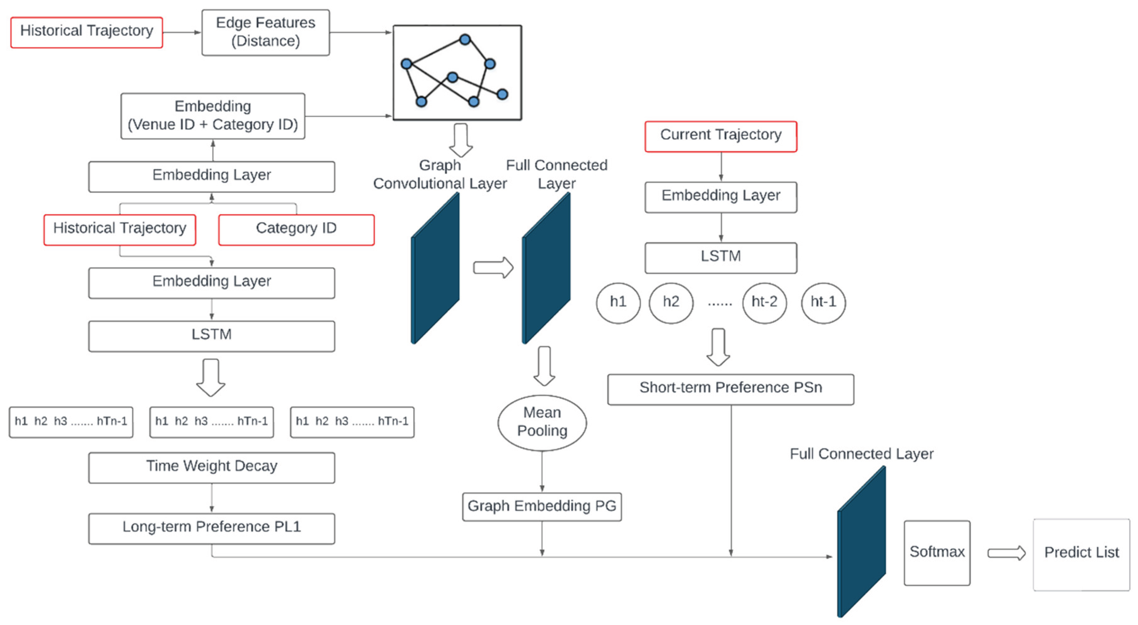

Table 1.
An example of next layer feature vectors.
| Node | adjacency list | distance | ||
|---|---|---|---|---|
| 0 | -1.1, 0.3, -0.1 | [0, 1], [0, 2] | 3, 2 | −0.439, 0.119, −0.040 |
| 1 | 0.6, 0.4, 0.4 | [1, 2], [1, 3] | 4, 1 | 0.34, 0.225, 0.225 |
| 2 | 0.5, 0.3, 0.5 | [0, 2], [1, 2] | 2, 1 | 0.34, 0.205, 0.34 |
| 3 | -1.0, 0.2, -0.1 | [1, 3], [3, 4], [3, 5] | 1, 4, 2 | -0.536, 0.103, -0.053 |
| 4 | -1.1, 0.3, -0.3 | [3, 4] | 4 | -0.26, 0.07, -0.07 |
| 5 | 0.5, 0.3, 0.3 | [3, 5] | 2 | 0.23, 0.14, 0.14 |
Table 2.
An example for Categorical Crossentropy.
| Sample | Label | Prediction | Loss |
|---|---|---|---|
| 1 | [1,0,0] | [0.8,0.1,0.1] | |
| 2 | [0,1,0] | [0.2,0.7,0.1] | |
| 3 | [0,0,1] | [0.1,0.3,0.6] |
Table 3.
dataset descriptions after preprocessing.
| Dataset | #of users | #of locations | # of categories |
|---|---|---|---|
| FourSquare NYC | 1083 | 8015 | 221 |
| FourSquare TKY | 2293 | 14508 | 203 |
Table 4.
The experimental results on dataset FourSquare NYC.
| Method | Evaluation Metric | K=1 | K=5 | K=10 |
|---|---|---|---|---|
| LSTPM | Recall | 0.0920 | 0.2920 | 0.3787 |
| NDCG | 0.0920 | 0.2227 | 0.2340 | |
| MAP | 0.0920 | 0.1999 | 0.2134 | |
| GLSP | Recall | 0.1737 | 0.3105 | 0.3882 |
| NDCG | 0.1737 | 0.2470 | 0.2720 | |
| MAP | 0.1737 | 0.2258 | 0.2360 | |
| STLGNet | Recall | 0.3049 | 0.5372 | 0.5852 |
| NDCG | 0.3049 | 0.5073 | 0.5225 | |
| MAP | 0.3049 | 0.4974 | 0.5035 |
Table 5.
The experimental results on dataset FourSquare TKY.
| Method | Evaluation Metric | K=1 | K=5 | K=10 |
|---|---|---|---|---|
| LSTPM | Recall | 0.0915 | 0.2691 | 0.3327 |
| NDCG | 0.0915 | 0.1920 | 0.2162 | |
| MAP | 0.0915 | 0.1669 | 0.1815 | |
| GLSP | Recall | 0.1153 | 0.2782 | 0.3514 |
| NDCG | 0.1153 | 0.1993 | 0.2230 | |
| MAP | 0.1153 | 0.1734 | 0.1831 | |
| STLGNet | Recall | 0.2302 | 0.3149 | 0.4868 |
| NDCG | 0.2302 | 0.2751 | 0.4615 | |
| MAP | 0.2302 | 0.2619 | 0.4234 |
Disclaimer/Publisher’s Note: The statements, opinions and data contained in all publications are solely those of the individual author(s) and contributor(s) and not of MDPI and/or the editor(s). MDPI and/or the editor(s) disclaim responsibility for any injury to people or property resulting from any ideas, methods, instructions or products referred to in the content. |
© 2025 by the authors. Licensee MDPI, Basel, Switzerland. This article is an open access article distributed under the terms and conditions of the Creative Commons Attribution (CC BY) license (http://creativecommons.org/licenses/by/4.0/).
Copyright: This open access article is published under a Creative Commons CC BY 4.0 license, which permit the free download, distribution, and reuse, provided that the author and preprint are cited in any reuse.


