Submitted:
28 September 2025
Posted:
29 September 2025
You are already at the latest version
Abstract
Autonomous navigation based on the stellar aberration effect derives the spacecraft’s velocity vector from the apparent stellar displacements. While promising, this technique is highly sensitive to distortions in the optical sensors onboard, requiring milliarcsecond-level correction. The plate-model method provides classical distortion correction, but formal uncertainties of plate constants depend on the number and spatial distribution of reference stars, catalog position errors, and sensor measurement noise. These uncertainties propagate through the plate model to the corrected positions of target stars, ultimately limiting the precision of the navigation observables. In this study, we systematically investigate the error-propagation mechanism of the plate model in the context of stellar-aberration navigation. We construct an all-sky simulated navigation catalog based on Gaia Date Release 3 and then establish a complete mathematical error-propagation chain from reference-star covariances to plate-constant solutions and finally to target-star positions. Adopting the six-constant plate model, we perform Monte Carlo simulations over the entire sky to quantify the influence of reference-star number and distribution on target-star positional precision. The results show that when more than ∼10 reference stars are available and well distributed within a field, the propagated plate-model error remains below 1 milliarcsecond, reaching 0.2–0.4 mas under favorable conditions. These findings demonstrate that plate-model errors are not the dominant limitation for stellar-aberration based autonomous navigation, provided that sufficient reference stars are included in the solution.
Keywords:
astrometry
; reference systems
; catalogs
; proper motions
; methods
; numerical simulation
1. Introduction
As deep-space exploration missions expand into increasingly distant and complex environments, the demand for autonomous navigation capabilities aboard spacecraft has become ever more pressing [1]. Traditional navigation modes that rely on ground-based deep-space tracking networks are constrained by communication delays and scarce tracking resources, and thus cannot satisfy the requirements of future missions for real-time, reliable, and autonomous navigation. Consequently, the development of astronomical autonomous navigation techniques that do not depend on ground support is of great strategic significance [2,3].
Among the various celestial navigation methods, the approach based on stellar aberration measures displacements in stellar apparent directions to directly infer the spacecraft velocity vector. This idea was formalized as the StarNAV concept by Christian [4], and subsequent studies have confirmed both the feasibility and observability of such a system [5]. Compared to celestial navigation using solar-system bodies, stellar-aberration navigation offers unique advantages: complete velocity observability, independence from specific bodies, and applicability across the entire sky. Moreover, the abundance of bright stars, together with the high astrometric precision provided by the Gaia mission, makes stellar aberration an attractive observable for autonomous navigation. Recent developments have further explored sensor architectures, fusion strategies, and adaptive filtering methods that enhance robustness and estimation accuracy [6]. Together, these studies highlight stellar aberration as an important research direction for future deep-space autonomous navigation.
In designing observational schemes for stellar-aberration-based navigation, the common modes fall into two categories: single-field or multi-field observations [4]. By measuring the angular separations between stars within a single field of view or across multiple fields, one can retrieve information about the spacecraft’s velocity. Therefore, achieving high-precision measurements of stellar directions is central to stellar aberration navigation. Previous studies have shown that, in order to reach a practically useful navigation accuracy, the stellar directional measurements often need to be better than 1 milliarcsecond (mas). This requires rigorous error control throughout all stages of observation and data processing. However, astrometric errors in stellar-aberration-based navigation have often been overlooked or underestimated in previous studies.
Recently, Zhang et al. [7] have demonstrated that the Gaia astrometric catalog from the European Space Agency space astrometry mission under the same name will remain the most accurate resource of stellar positions for the next 20–30 years, making it the preferred input catalog for autonomous celestial navigation missions. Evaluations based on Gaia Data Release 3 (DR3) [8,9] indicate that for stars brighter than , the typical positional accuracy of navigation stars is about mas at epoch J2025.0, and remains better than mas at epoch J2040.0. This fully satisfies the mas accuracy requirement for navigation.
However, geometric distortion existing in the optical system onboard is non-negligible. It causes the measured positions of stars on the focal plane (measured coordinates) to deviate from their theoretical distortion-free positions (standard coordinates), with deviations reaching the milliarcsecond level or higher [10]. Without precise correction, such distortion can overwhelm the subtle stellar aberration signal and prevent reliable navigation solutions.
In photographic astrometry, the plate constant method is a classical and effective technique for correcting optical distortion. Its central idea is to use a set of reference stars with known positions within the field of view to establish a mathematical transformation between the measured coordinates and the standard coordinates , namely the plate model. The unknown parameters of this model are called plate constants. By observing the reference stars, one can solve for the plate constants using least-squares or similar methods. Once the plate constants are determined, the model can be applied to transform the measured coordinates of any target star within the field into standard coordinates, thereby removing the effects of optical distortion.
However, the solution of the plate constants itself introduces errors. These errors mainly arise from three sources: (i) positional errors of reference stars in the catalog; (ii) measurement noise in the measured coordinates of reference stars; (iii) the limited number and uneven distribution of reference stars within the field, which leads to ill-conditioned model equations. These factors cause the estimated plate constants to deviate from their true values, producing plate model errors. When this erroneous model is applied to correct target star positions, the errors propagate into the target’s standard coordinates, ultimately degrading the accuracy of the navigation observables. This type of error is termed the plate constant variance in Eichhorn and Williams [11], which represents the systematic lower bound of plate model error.
Plummer [12] was the first to study plate constant variance. By analyzing the normal equations for the four-constant and six-constant solutions, he found that the variance is inversely proportional to the square of the number of reference stars within the field. Eichhorn and Williams [11] explicitly introduced the concept of “plate constant variance” and, under a simple assumption regarding the distribution of reference stars, derived an analytical expression for it. Later, other authors such as von der Heide [13] and Scholz et al. [14] extended the analysis to more complex cases, including errors introduced by overlapping plates. Different formalisms of the plate model, such as quaternions [15] and orthogonal functions [e.g.; [16,17,18] were also explored to imporove the systematic accuracy of the solution. However, these studies cannot be directly applicable to stellar-aberration-based navigation.
This paper aims to systematically evaluate the plate model errors in stellar aberration navigation, following the error modeling proposed in Eichhorn and Williams [11]. By constructing a complete error propagation model, we quantitatively analyze the magnitude of errors introduced by the plate model under different observational conditions. The main steps include: (1) building a high-precision navigation star catalog based on the latest Gaia data (Sect. 2); (2) establishing a mathematical model and simulation pipeline for error propagation from reference star errors to plate constant errors and then to target star position errors (Sect. 3); (3) conducting an in-depth analysis of how the number and distribution of reference stars affect the final target star positional accuracy (Sect. 4). The final goal is to answer the key question, that is, whether plate model errors are the principal limiting factor in the accuracy of stellar-aberration-based navigation.
Throughout the paper, we assume the designed optical sensors onboard has a field of view of with a limiting magnitude of ∼ 10 mag. The stellar magnitudes refer to the G-band magnitudes (wavelength coverage 330–1050 nm) used in the Gaia catalog. The astrometric measurement noise is assumed to be 1 mas, as done in Christian [4].
2. Preparation of the Reference Star Catalog
An accurate navigation reference catalog is an essential input for simulation in this work. We adopt the Gaia DR3 from as the base catalog [9]. With sub-milliarcsecond astrometric precision, Gaia DR3 represents the most accurate and comprehensive resource currently available for constructing a high-accuracy navigation star catalog [19]. We select stars with as candidate navigation stars, consistent with the assumed limiting sensitivity of the optical sensor. This resulted in a catalog of 477,502 navigation stars, corresponding to an average sky density of about 12 stars per square degree.
2.1. HEALPix Pixelization
To facilitate simulations in different sky regions, we divide the celestial sphere using the Hierarchical Equal Area isoLatitude Pixelization (HEALPix) scheme [20]. We adopt a resolution parameter of (corresponding to order ), which partitions the full sky into equal-area pixels. Each pixel covers a solid angle of
corresponding to an effective angular scale of . This resolution is well matched to the field of view of the designed optical instrument. In our subsequent simulations, each HEALPix pixel is treated as an independent observational field.
As illustrated in the map of stellar density (Figure 1), the number of navigation stars is strongly correlated with Galactic latitude: stellar densities are much higher along the Galactic plane than near the poles. Nearly half of the sky pixels contain more than 20 stars, providing ample references for solving plate model parameters.
2.2. Epoch Propagation of Navigation Star Positions
The reference epoch of the Gaia DR3 catalog is . For a stellar-aberration-based navigation mission assumed to take place at , the catalog positions must be propagated to this epoch. The relevant astrometric parameters provided by Gaia are , where and are the proper motions in right ascension (corrected by a factor of ) and declination. Neglecting parallax and radial velocity terms, the celestial coordinates of a star at epoch t are
Linearizing with respect to the catalog parameters yields the Jacobian matrix
If the Gaia catalog provides the covariance matrix of the astrometric parameters, , the propagated covariance of the celestial coordinates at epoch t is
For a single navigation star, this covariance matrix takes the form
The total positional uncertainty is defined as the semi-major axis of the error ellipse, i.e. the square root of the largest eigenvalue of the covariance matrix [21]:
Figure 2 shows the distribution of positional uncertainties for all stars in the navigation catalog propagated to epoch J2026.0. The vast majority () of stars have positional uncertainties below 0.4 mas. The median uncertainties in right ascension () and declination () are both mas, comfortably meeting the accuracy requirements for stellar-aberration navigation and plate modeling.
3. Simulation of Plate-Model Error Propagation
3.1. Projection and Plate Model
Standard (distortion-free) sky coordinates are defined on the tangent plane via a gnomonic projection, centered on the optical axis of the field of view. For each field, we take the HEALPix pixel center as the projection origin. The standard tangent-plane coordinates of a star at equatorial coordinates are then given by the gnomonic projection [22]:
The plate model describes the mapping between the standard tangent-plane coordinates and the measured focal-plane coordinates . To maintain consistent units and simplify error propagation, x and y are expressed in angular units (arcsec) on the tangent plane. The six-constant linear plate model [11] is
where are all in arcseconds, C and (arcsec) represent translations of the coordinate origin, and (dimensionless) account for the scale, rotation, and possible axis skew. To emulate realistic instrument distortion, we adopt parameters measured for the Hubble Space Telescope [10], which are
3.2. Plate-Model Error Propagation
The standard coordinates and the measured coordinates of navigation (reference) stars can be expressed in an approximate linear observation equation:
where denotes the vector of standard tangent-plane coordinates of the reference stars, is the design matrix formed from the measured focal-plane coordinates, and is the vector of plate-model parameters. For the six-constant model we have
and represents the combined perturbation from catalog errors and measurement noise.
For the i-th reference star with standard coordinates and measured coordinates , the six-constant plate model can be written as
Stacking the equations for N reference stars gives
In a least-squares solution, the covariance matrix of the estimated plate parameters is . For a target star with measured coordinates , the corresponding design row is . The covariance of its propagated tangent-plane coordinates is then
with diagonal elements giving the variances and . The total astrometric error in the target-star position due to plate-constant variance is
This formulation follows the classical treatment of plate-constant variance [e.g.; [11,23], and provides the basis for quantifying how positional uncertainties in the navigation catalog and measurement noises of reference stars propagate to the target star position. Figure 3 summarizes the error propagation and analysis chain as described above.
4. Simulation Results and Analysis
4.1. Single-Star Simulation: Barnard’s Star
To illustrate the combined effects of catalog errors, measurement noise, and field distortion on measured coordinates, we use Barnard’s Star as a representative single-star case and perform Monte Carlo simulations. At epoch J2026.0, Barnard’s Star has equatorial coordinates and , with the propagated uncertainties of in right ascension and in declination, and a correlation coefficient of between the two. The covariance matrix describing the catalog position uncertainty is
from which we draw random offsets from a zero-mean bivariate normal distribution. Figure 4a displays the results of simulated position offsets , along with confidence ellipses corresponding to the 1- (68.3%), 2- (95.4%), and 3- (99.7%) levels. These positions are then projected onto the tangent plane centered on the field origin using Eqs. (6)–(7) to obtain the standard coordinates . The distribution after projection is shown in Figure 4b. Because the gnomonic projection is nearly linear in the vicinity of the tangent point, the shape and orientation of the distribution remain consistent with Figure 4a, representing the dispersion due solely to catalog errors.
As stated before, the measurement noise is modeled as a zero-mean bivariate normal distribution with standard deviations of in both x and y, and no correlation between axes. Figure 4c shows noise realizations . Finally, the simulated catalog and measurement uncertainties are combined under three scenarios:
- With distortion and noise: distorted coordinates are further perturbed by measurement noise. The final distribution in Figure 4f represents the simulated measured coordinates of Barnard’s Star in a realistic navigation observation.
While the Barnard’s Star example illustrates how catalog errors, measurement noise, and distortion combine for a single star, the same framework can be applied to all HEALPix fields across the sky. In the following analysis, we uniformly adopt the six-constant plate model and a representative measurement error of .
4.2. Plate-Model Error Distribution in a Representative Field
We select the pixel field containing Barnard’s Star (HEALPix ID 31781) as a representative FOV for detailed analysis (Figure 5). This field contains 20 reference stars with mag. Using the simulated reference-star data, we solve for the plate-model parameters. From Monte Carlo realizations, we obtain the empirical distributions of the six plate constants (Figure 6). The dispersion in each panel directly reflects the uncertainty of the corresponding parameter estimate, determined jointly by the geometric configuration of reference stars, their catalog errors, and measurement noise. From these solutions we compute the covariance matrix of the plate constants, that is, .
Within the FOV we evaluate a grid with 1 arcmin spacing. At each grid point, we propagate the plate-constant covariance to estimate the target-star positional errors. Figure 7 depicts the spatial distribution of errors in the two standard-coordinate components and in total. The plate-model-induced error is clearly non-uniform: errors are smallest near the field center, where reference-star coverage is dense, but grow substantially toward the edges and corners where references are sparse. As seen in Figure 7c, the overall position error remains below in the central region but increases steeply to above in the corners. When a target lies outside the geometric hull formed by nearby reference stars, the model uncertainty is amplified, producing larger positional errors. This behavior is consistent with the findings of Eichhorn and Williams [11], who showed that plate-constant variance grows rapidly toward the plate boundaries.
To achieve high-precision positioning, the target should be as well surrounded by reference stars as possible, avoiding edge regions of the reference-star distribution. In multi-field observing modes, selecting targets closest to the field center generally ensures that plate-model error does not dominate the stellar-aberration observable. In single-field observations, however, maximizing the weak aberration signal often favors stars near the field extremes, where the plate-constant variance may exceed . In such cases, plate-model errors cannot be neglected, and careful selection of star pairs and imaging schedules becomes essential.
A comparison of Figure 7a,b further shows that the error patterns in and differ, reflecting the asymmetric geometry of the reference stars. For example, along the upper and lower edges of the FOV, the -direction error (peaking at ) is generally larger than the -direction error (peaking at ), indicating weaker horizontal than vertical constraint in those regions. The true level of plate-constant variance is thus governed by a complex interplay of geometry, catalog accuracy, and measurement noise, defying simple analytic characterization but accessible through numerical simulation.
4.3. All-Sky Distribution of Plate-Model Errors
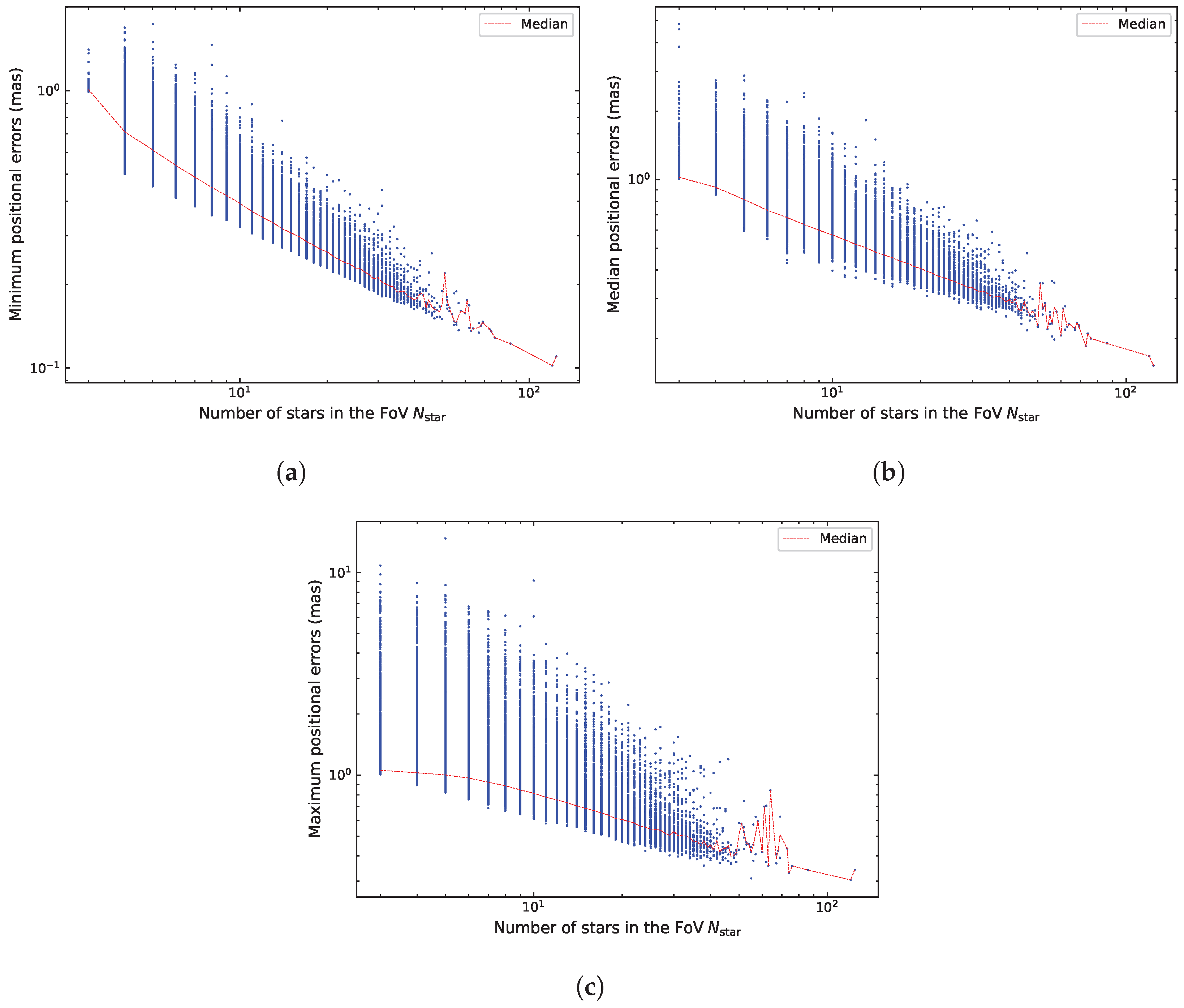
To assess the impact of reference-star density on plate-constant variance, we simulate all sky fields that contain at least three navigation stars (to enable a least squares fitting). For each field, we compute the minimum, median, and maximum positioning errors across all target stars to represent best-case, typical, and worst-case scenarios. Figure 8 presents how these statistics vary with the number of reference stars . In all three cases, the plate-model–induced positional error decreases nearly linearly (in log–log space) with increasing .
According to the median statistics in Figure 8b, when only reference stars are available, the typical positional error is at the level. Increasing the number of reference stars to steadily reduces the median error to , and for , the median error can be driven below . The maximum-error trend in Figure 8c highlights the worst-case precision within a field. Even with many reference stars (), unfavorable spatial configurations may yield edge targets with errors exceeding . Nevertheless, increasing the number of reference stars is the most effective way to suppress such extremes: raising the count from 10 to 40 reduces the median of the maximum error from a few to below .
From a global perspective, we also compile statistics of plate-constant variance for all navigation stars across the sky. Figure shows the histogram of these errors, which exhibits a prominent peak between and , with 77.18% of stars below the threshold. These stars therefore meet the accuracy requirement for stellar-aberration navigation and are qualified as viable navigation targets.
5. Conclusions
In this work, we carried out systematic modeling, simulation, and quantitative analysis of plate-model errors in stellar-aberration–based autonomous spacecraft navigation. We first constructed a navigation reference catalog based on Gaia DR3, propagating stellar positions to a fixed epoch and retaining both positions and their covariance information, thereby providing the input data source for subsequent error propagation. We then established a well-defined error-propagation chain: catalog covariances and measurement noise enter the observation equations; the plate model is fitted to obtain plate parameters and their covariance; and a Jacobian matrix propagates the parameter uncertainties to the standard coordinates of target stars, yielding the mathematical expression for plate-constant variance. Finally, adopting the six-constant plate model, we performed Monte Carlo simulations to quantify the influence of both the number and spatial distribution of reference stars on the precision of navigation observables.
Our results show that when a sufficient number of reference stars () are available and well distributed, the plate-constant variance remains below and can reach –. However, when reference stars are sparse or unevenly distributed, extrapolation effects accumulate and the errors in edge regions rise to the 1– level. This imposes stricter requirements on observational planning and field selection for stellar-aberration navigation. On a global scale, more than 70% of candidate navigation stars exhibit plate-constant variance below , indicating that plate-model errors are not the principal factor limiting the accuracy of stellar-aberration navigation when the six-constant solution is used.
Future work will extend this framework to alternative measurement strategies based on relative stellar separations, which may offer enhanced internal precision but also require careful treatment of differential aberration and other systematic effects. Such developments will further strengthen the reliability of astrometric methods for autonomous deep-space navigation.
Author Contributions
Conceptualization, M.L. and N.L.; methodology, N.L. and D.Z.; validation, D.Z., M.L. and N.L.; formal analysis, D.Z. and N.L.; investigation, N.L.; writing—original draft preparation, D.Z. and N.L.; writing—review and editing, M.L. and N.L.; visualization, N.L.; funding acquisition, M.L. All authors have read and agreed to the published version of the manuscript.
Funding
This research was funded by the National Natural Science Foundation of China (NSFC) grant number 125B1029 and the Natural Science Foundation of Shanghai grant number 24ZR1429100.
Institutional Review Board Statement
Not applicable.
Informed Consent Statement
Not applicable.
Data Availability Statement
The original data presented in the study are openly available at https://git.nju.edu.cn/astrometry/plate_model_error.
Acknowledgments
This work has made use of data from the European Space Agency (ESA) mission Gaia (https://www.cosmos.esa.int/gaia), processed by the Gaia Data Processing and Analysis Consortium (DPAC, https://www.cosmos.esa.int/web/gaia/dpac/consortium). Funding for the DPAC has been provided by national institutions, in particular the institutions participating in the Gaia Multilateral Agreement.
Conflicts of Interest
The authors declare no conflicts of interest.
References
- McKee, P.; Kowalski, J.; Christian, J.A. Navigation and star identification for an interstellar mission. Acta Astronautica 2022, 192, 390–401. [Google Scholar] [CrossRef]
- Fang, J.; Ning, X.; Ma, X.; Liu, J.; Gui, M. A survey of autonomous astronomical navigation technology for deep space detectors. Flight Control & Detection 2018, 1, 1–15. [Google Scholar]
- Zhang, W.; Xu, J.; Huang, Q.; Chen, X. Survey of Autonomous Celestial Navigation Technology for Deep Space. Flight Control & Detection 2020, 8–16. [Google Scholar]
- Christian, J.A. StarNAV: Autonomous Optical Navigation of a Spacecraft by the Relativistic Perturbation of Starlight. Sensors 2019, 19, 4064. [Google Scholar] [CrossRef] [PubMed]
- Li, M.; Sun, J.; Peng, Y.; Liu, J. Observability and Performance Analysis of Spacecraft Autonomous Navigation Using Stellar Aberration Observation. In Proceedings of the 2021 5th International Conference on Vision, Image and Signal Processing (ICVISP), Kuala Lumpur, Malaysia; 2021; pp. 218–223. [Google Scholar] [CrossRef]
- Xiong, K.; Wei, C.; Zhou, P. Integrated Autonomous Optical Navigation Using Q-Learning Extended Kalman Filter. Aircraft Engineering and Aerospace Technology: An International Journal 2022, 94, 848–861. [Google Scholar] [CrossRef]
- Zhang, D.; Li, M.; Liu, N. Construction of Aberration Navigation Catalog Based on the Gaia Catalog. Flight Control & Detection 2025. In press. [Google Scholar]
- Gaia Collaboration; Prusti, T.; de Bruijne, J.H.J.; Brown, A.G.A.; Vallenari, A.; Babusiaux, C.; Bailer-Jones, C.A.L.; Bastian, U.; Biermann, M.; Evans, D.W.; et al. The Gaia mission. A&A 2016, 595, A1, [arXiv:astro-ph.IM/1609.04153]. [Google Scholar] [CrossRef]
- Gaia Collaboration; Brown, A.G.A.; Vallenari, A.; Prusti, T.; de Bruijne, J.H.J.; Babusiaux, C.; Biermann, M.; Creevey, O.L.; Evans, D.W.; Eyer, L.; et al. Gaia Early Data Release 3. Summary of the contents and survey properties. A&A 2021, 649, A1, [arXiv:astro-ph.GA/2012.01533]. [Google Scholar] [CrossRef]
- Kozhurina-Platais, V.; Grogin, N.A.; Sabbi, E. Astrometric Calibrations of HST Images in the Era of Gaia. In Proceedings of the American Astronomical Society Meeting Abstracts #232, 2018, Vol. 232, American Astronomical Society Meeting Abstracts, p. 119.13.
- Eichhorn, H.; Williams, C.A. On the systematic accuracy of photographic astrographic data. AJ 1963, 68, 221–231. [Google Scholar] [CrossRef]
- Plummer, H.C. Note on the Influence of the Plate Constants on the Accuracy of the Position of an Object measured on a Photograph. MNRAS 1904, 64, 645. [Google Scholar] [CrossRef]
- von der Heide, K. On the reduction model of astrographic plates. A&A 1979, 72, 324–331. [Google Scholar]
- Scholz, R.D.; Odenkirchen, M.; Hirte, S.; Irwin, M.J.; Borngen, F.; Ziener, R. Absolute proper motions and Galactic orbits of M5, M12 and M15 from Schmidt plates. MNRAS 1996, 278, 251–264. [Google Scholar] [CrossRef]
- Jefferys, W.H. Quaternions as Astrometric Plate Constants. AJ 1987, 93, 755. [Google Scholar] [CrossRef]
- Bienayme, O. Field astrometry using orthogonal functions. A&A 1993, 278, 301–306. [Google Scholar]
- Makarov, V.V.; Veillette, D.R.; Hennessy, G.S.; Lane, B.F. The Worst Distortions of Astrometric Instruments and Orthonormal Models for Rectangular Fields of View. PASP 2012, 124, 268, [arXiv:astro-ph.IM/1110.2967]. [Google Scholar] [CrossRef]
- Peng, H.W.; Peng, Q.Y.; Wang, N. An improved solution to geometric distortion using an orthogonal method. Research in Astronomy and Astrophysics 2017, 17, 21, [arXiv:astro-ph.IM/1612.05801]. [Google Scholar] [CrossRef]
- Lindegren, L.; Klioner, S.A.; Hernández, J.; Bombrun, A.; Ramos-Lerate, M.; Steidelmüller, H.; Bastian, U.; Biermann, M.; de Torres, A.; Gerlach, E.; et al. Gaia Early Data Release 3. The astrometric solution. A&A 2021, 649, A2, [arXiv:astro-ph.IM/2012.03380]. [Google Scholar] [CrossRef]
- Górski, K.M.; Hivon, E.; Banday, A.J.; Wandelt, B.D.; Hansen, F.K.; Reinecke, M.; Bartelmann, M. HEALPix: A Framework for High-Resolution Discretization and Fast Analysis of Data Distributed on the Sphere. ApJ 2005, 622, 759–771. [Google Scholar] [CrossRef]
- Lindegren, L.; Lammers, U.; Bastian, U.; Hernández, J.; Klioner, S.; Hobbs, D.; Bombrun, A.; Michalik, D.; Ramos-Lerate, M.; Butkevich, A.; et al. Gaia Data Release 1. Astrometry: one billion positions, two million proper motions and parallaxes. A&A 2016, 595, A4, [arXiv:astro-ph.GA/1609.04303]. [Google Scholar] [CrossRef]
- Van Altena, W.F. Astrometry for astrophysics: methods, models, and applications; Cambridge University Press: Cambridge, UK, 2013. [Google Scholar]
- Zheng, Z.J.; Peng, Q.Y.; Lin, F.R. Using Gaia DR2 to make a systematic comparison between two geometric distortion solutions. MNRAS 2021, 502, 6216–6224, [arXiv:astro-ph.IM/2108.10478]. [Google Scholar] [CrossRef]
Figure 1.
All-sky density distribution of navigation stars from Gaia DR3 ( mag), pixelized with HEALPix at (pixel area deg2). The color scale indicates the number of stars per pixel.
Figure 1.
All-sky density distribution of navigation stars from Gaia DR3 ( mag), pixelized with HEALPix at (pixel area deg2). The color scale indicates the number of stars per pixel.
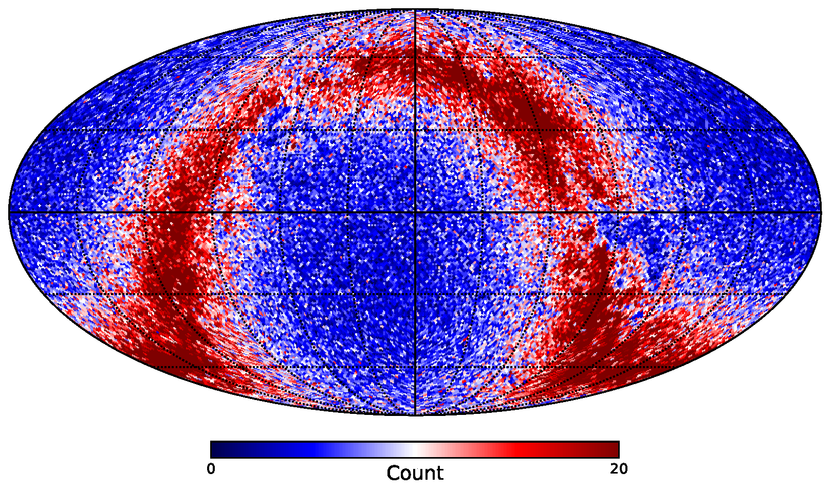
Figure 2.
Histograms of positional uncertainties in the navigation star catalog at J2026.0: red shows total positional uncertainty, blue right ascension, and green declination.
Figure 2.
Histograms of positional uncertainties in the navigation star catalog at J2026.0: red shows total positional uncertainty, blue right ascension, and green declination.
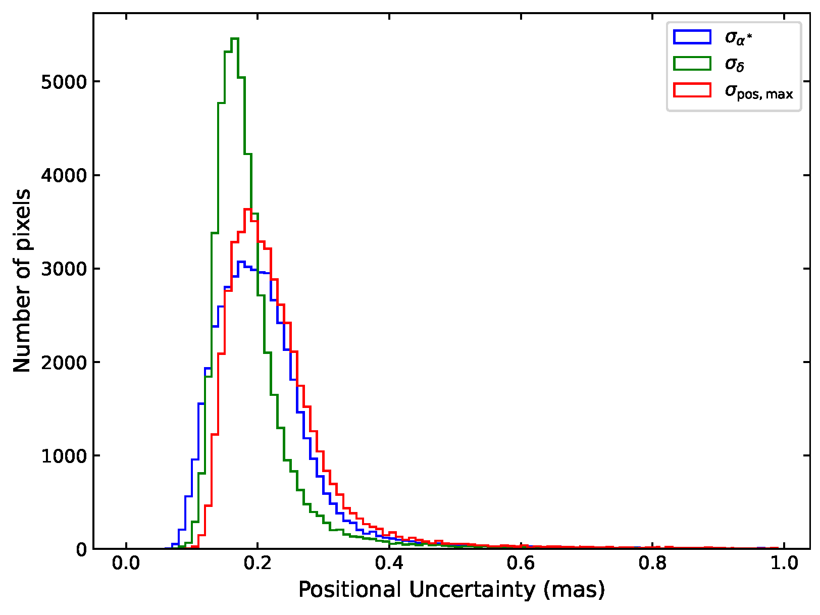
Figure 3.
Flowchart of the Monte Carlo simulation used for error propagation analysis.
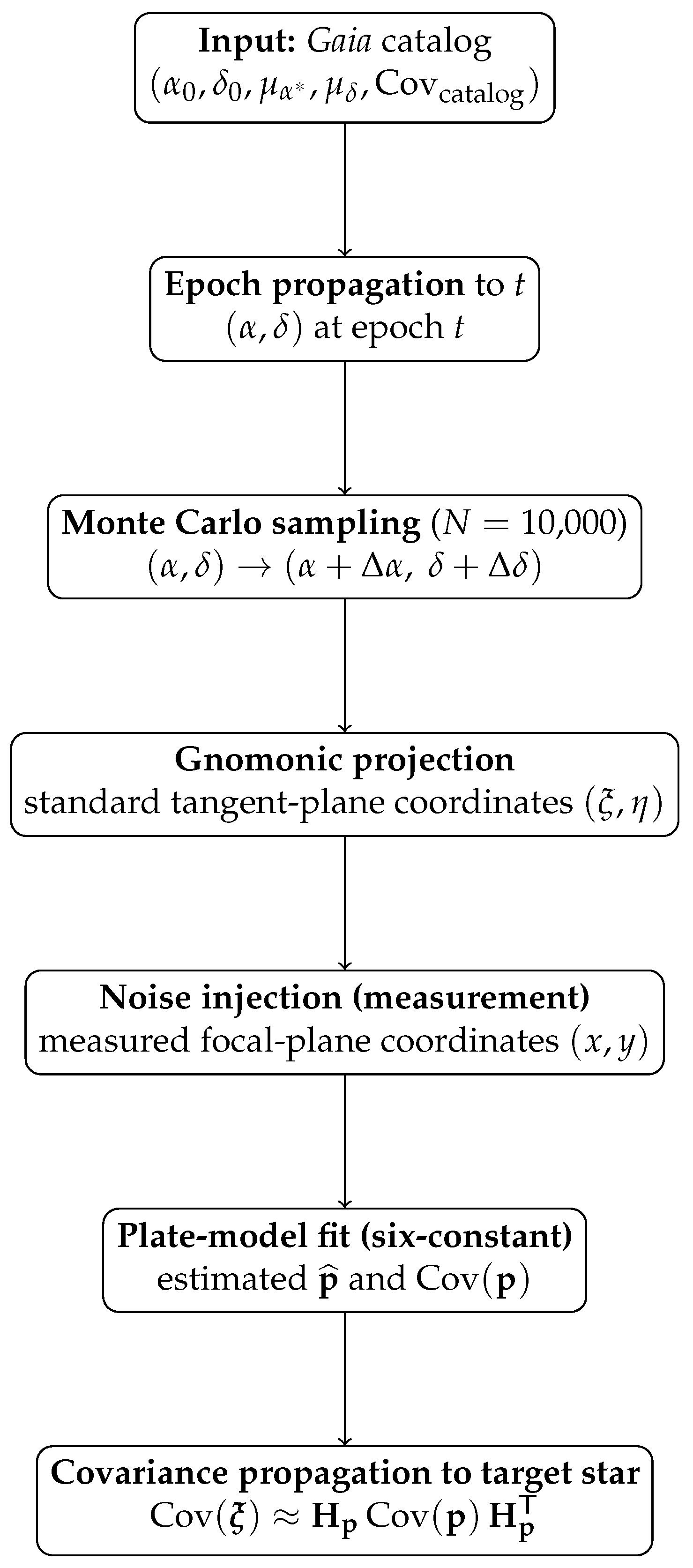
Figure 4.
Monte Carlo simulation of measured coordinates for Barnard’s Star at epoch J2026.0. (a) Catalog position uncertainty with – confidence ellipses. (b) Projection of catalog errors into standard tangent-plane coordinates . (c) Measurement noise with mas per axis. (d) Combined effect of catalog error and measur noise without distortion. (e) Effect of distortion alone using a representative plate model. (f) Combined effect of distortion and measur noise, representing the final measured coordinates.
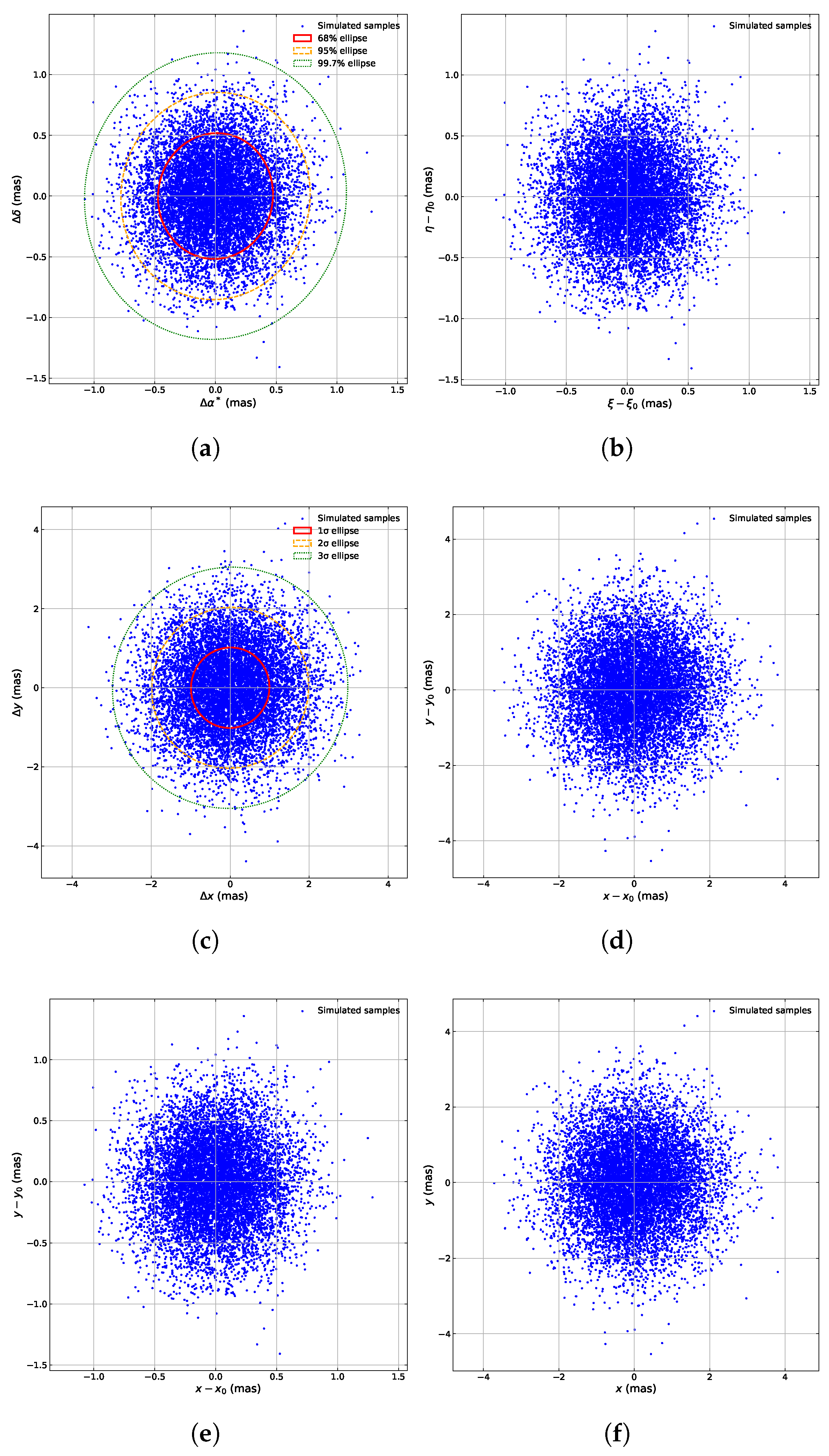
Figure 5.
Distribution of reference stars in the target HEALPix field (ID 31781). Point shading encodes Gaia G magnitude, with darker symbols indicating brighter stars. This field contains 20 reference stars with mag.
Figure 5.
Distribution of reference stars in the target HEALPix field (ID 31781). Point shading encodes Gaia G magnitude, with darker symbols indicating brighter stars. This field contains 20 reference stars with mag.
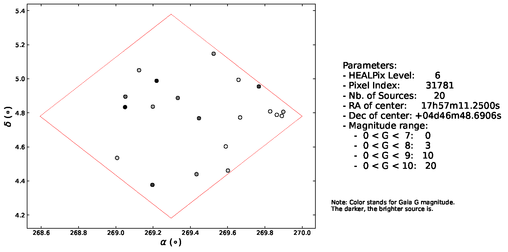
Figure 6.
Empirical distributions of the six plate constants () from Monte Carlo solutions in the representative HEALPix field (ID 31781).
Figure 6.
Empirical distributions of the six plate constants () from Monte Carlo solutions in the representative HEALPix field (ID 31781).
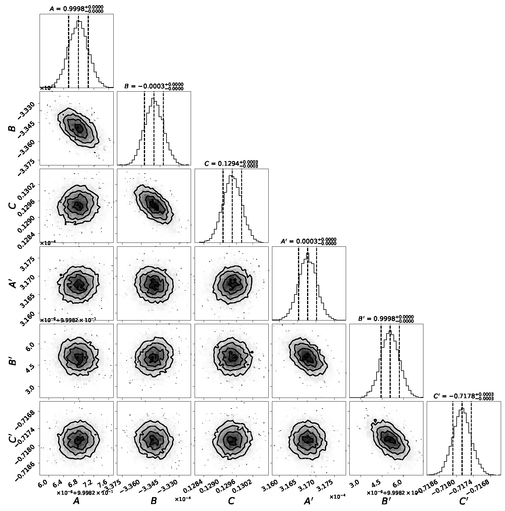
Figure 7.
Spatial distribution of plate-model–induced errors in the representative HEALPix field (ID 31781). (a) Propagated error components in the standard coordinate . (b) Propagated error components in the standard coordinate . (c) Total position error . Coordinate axes are in arcminutes, and the color scale gives positional error in mas.
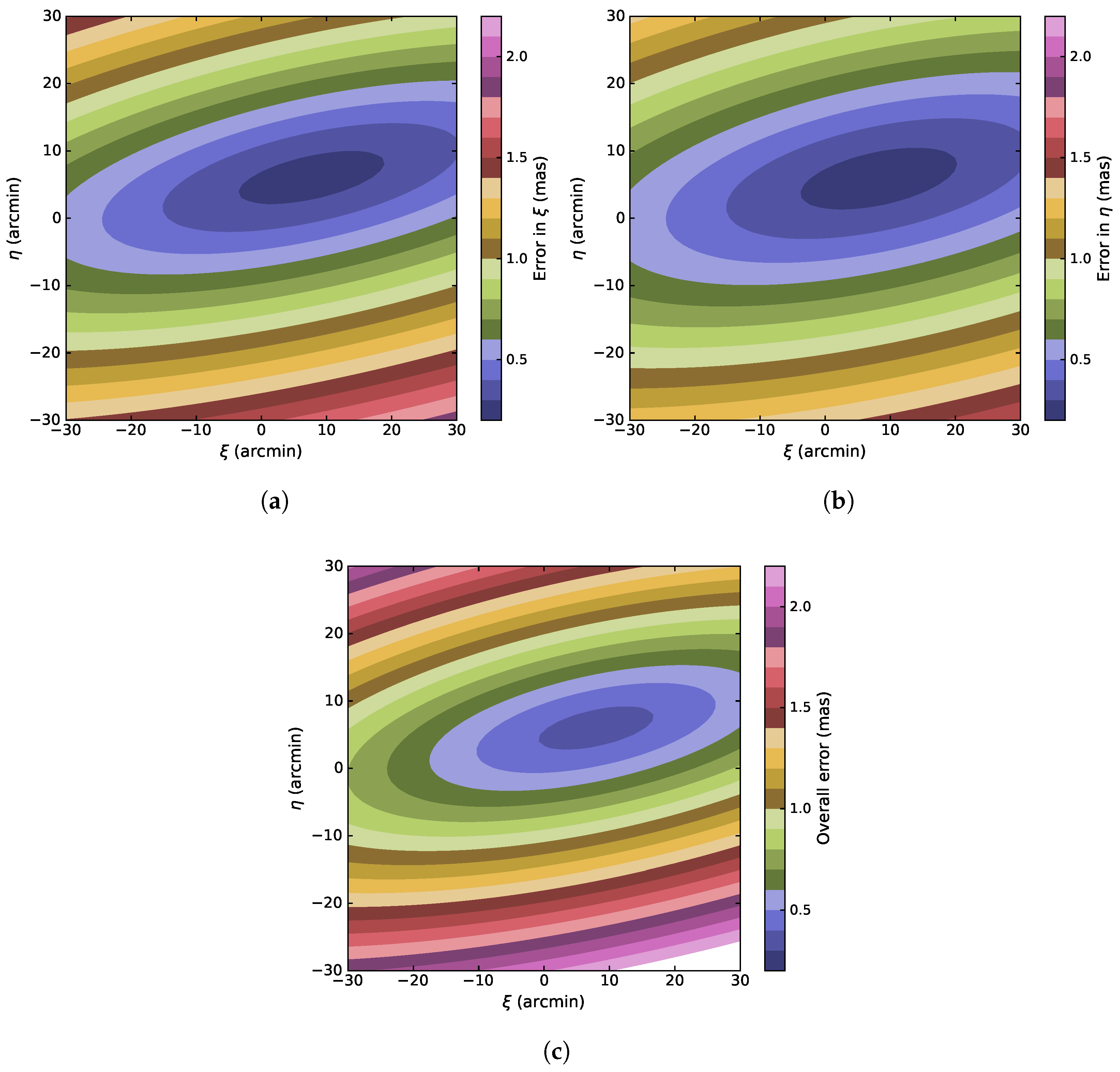
Figure 8.
Plate-model–induced positional errors as a function of the number of reference stars per field. Each point represents the simulation result for an independent HEALPix field. Both axes are shown on logarithmic scales. The red dashed lines indicate the median value of each bin. (a) Minimum error (best case). (b) Median error (typical case). (c) Maximum error (worst case).
Disclaimer/Publisher’s Note: The statements, opinions and data contained in all publications are solely those of the individual author(s) and contributor(s) and not of MDPI and/or the editor(s). MDPI and/or the editor(s) disclaim responsibility for any injury to people or property resulting from any ideas, methods, instructions or products referred to in the content. |
© 2025 by the authors. Licensee MDPI, Basel, Switzerland. This article is an open access article distributed under the terms and conditions of the Creative Commons Attribution (CC BY) license (http://creativecommons.org/licenses/by/4.0/).
Copyright: This open access article is published under a Creative Commons CC BY 4.0 license, which permit the free download, distribution, and reuse, provided that the author and preprint are cited in any reuse.


