Submitted:
26 September 2025
Posted:
02 October 2025
You are already at the latest version
Abstract
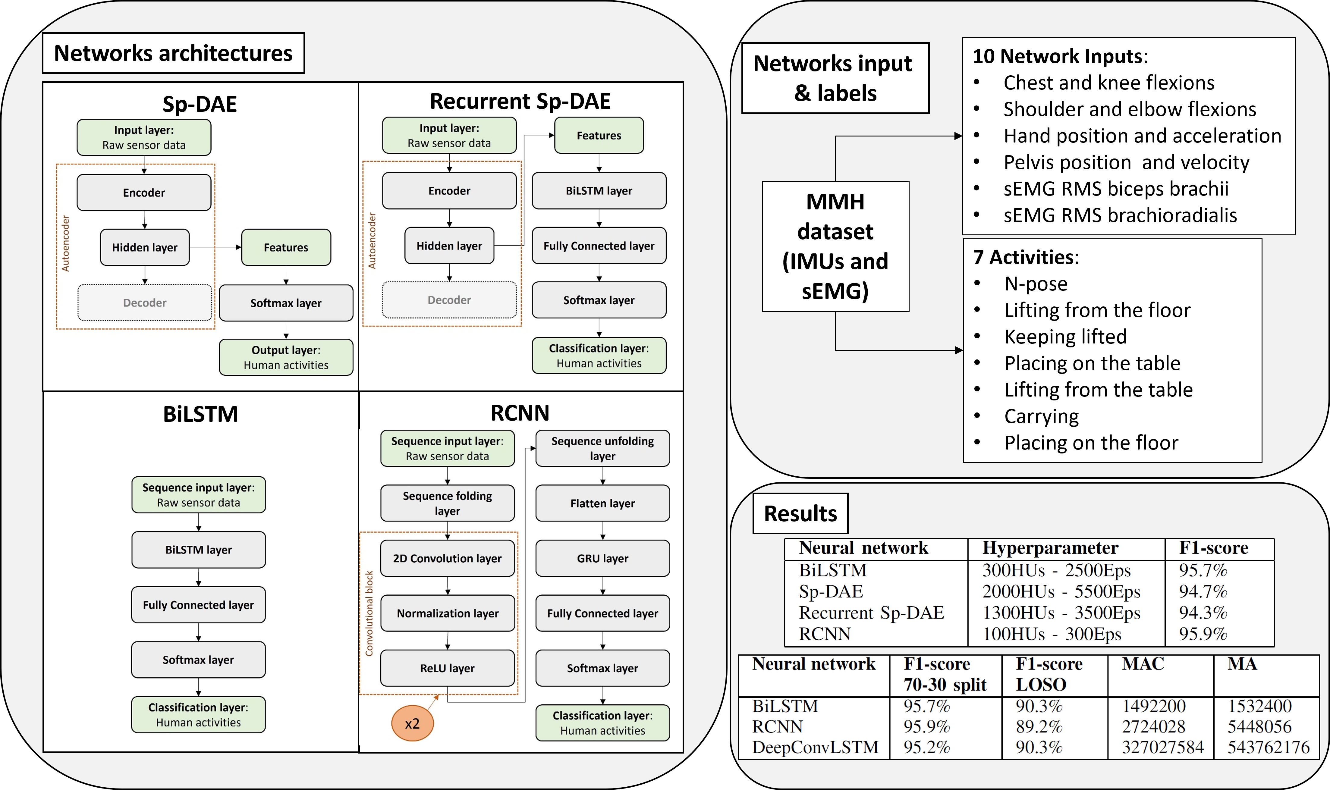
Human Activity Recognition (HAR) is widely used for healthcare, but few works focus on Manual Material Handling (MMH) activities, despite their diffusion and impact on the workers’ health. We propose four Deep Learning algorithms for HAR in MMH: Bidirectional Long Short-Term Memory (BiLSTM), Sparse Denoising Autoencoder (Sp-DAE), Recurrent Sp-DAE; and Recurrent Convolutional Neural Network (RCNN). We explored different hyperparameter combinations to maximize the classification performance (F1-score) using wearable sensors’ data gathered from 14 subjects. We investigated the best three-parameter combinations for each network using the full dataset to select the two best-performing networks, that were then compared using 14 datasets with increasing subject numerosity, 70%-30% split and Leave-One-Subject-Out (LOSO) validation, to evaluate whether they may perform better with a larger dataset. The benchmarking network DeepConvLSTM was tested on the full dataset. BiLSTM performs best in classification and complexity (95.7% 70%-30% split, 90.3% LOSO). RCNN performed similarly (95.9%, 89.2%) with a positive trend with subject numerosity. DeepConvLSTM achieves similar classification performance (95.2%, 90.3%) requiring more than 100 greater Multiply and ACcumulate and Multiplication and Addition operations, which measure the networks’ complexity. The BILSTM and RCNN perform close to DeepConvLSTM while being much computationally lighter, fostering their use in embedded systems. Such lighter algorithms can be readily used in the automatic ergonomic and biomechanical risk assessment systems, enabling personalization of risk assessment and easing the adoption of safety measures in industrial practices involving MMH.
Keywords:
Autoencoder
; Convolutional Neural Network (CNN)
; Human Activity Recognition (HAR)
; Manual Material Handling (MMH)
; Recurrent Neural Network (RNN)
; Wearable Sensor Network (WSN)
1. Introduction
Human Activity Recognition (HAR) is the task of classifying agents’ actions based on sensor data. The knowledge of human behaviors has potential applications in many fields, such as ambient-assisted living [1], rehabilitation [2], industrial tasks safety [3], and Human-Robot Interaction (HRI) [4]. In the view of Industry 4.0, smart automation is permeating traditional industrial practices aiming at increasing productivity while improving operators’ working conditions. In this context, humans and robots collaborate on the same tasks in a shared workplace [5] and Manual Material Handling (MMH) activities are expected to remain dominant in many industrial fields. These occupations expose workers to high biomechanical risks that frequently induce Work-related Musculoskeletal Disorders (WMSDs) [6]. Therefore, the automatization of the WMSDs risk assessment is the key to guaranteeing workers’ health.
To this end, HAR algorithms, determining which action led to specific measures in the sensor data streams, allow automatizing the workplace ergonomics and biomechanical evaluation processes [7]. Sensor data classified by HAR algorithms can come from external devices, such as cameras, or wearable sensors. The latters are generally preferred because of their flexibility, portability, and unobtrusiveness [8,9]. In particular, Inertial Measurement Units (IMUs) are commonly used since they are small, affordable, and available in many commercial goods. Superficial Electromyography (sEMG) signals are valuable complements of IMUs, as they provide many parameters regarding muscle contractions and contain information on the movement intentions of the subject wearing the device [10]. Moreover, sEMG signals allow recognizing movements [11], evaluating muscle forces, and predicting handled loads [12], desirable features for both ergonomic assessment and robot control in human-robot shared tasks.
Many Machine Learning (ML) techniques, such as Support Vector Machine, K-Nearest Neighbour, Hidden Markov Models, Gaussian Mixture Model, Decision Tree, and Bayes Network have been employed in HAR [13]. One of the main challenges that ML techniques need to face is the complexity of the extraction of the more discriminative features especially because various actions can be very similar to each other (inter-activity similarity), the same action can be performed differently from person to person (intra-activity variability), the sensors types and their placements highly influence the data streams obtained (sensor variability), and often the activities can be considered as composite or concurrent. Despite the notable evolution of ML methods, there is no universal approach for selecting the best feature set representing human activities, and this process is highly demanding and time-consuming. To solve this issue, Deep Learning (DL) methods have the potential to model high-level abstraction from complex data, reducing the workload of feature selection [9]. In HAR applications, DL proved its ability to solve the problems of intra-activity variability and inter-activity similarity [14]. Various deep neural network structures have been used to highlight different characteristics of the input sequences [15], which include Convolutional Neural Networks (CNNs), Recurrent Neural Networks (RNNs), and Feedforward Neural Networks (FNNs) such as Autoencoders.
Nowadays, most ML and DL research applied to HAR regards locomotion or Activities of Daily Living (ADLs) [16]. State-of-the-Art (SoA) HAR studies in industrial applications mainly focus on assembling and packaging activities [17], whereas only a few works regard MMH activities. In addition, most of these works adopt ML methods [18,19] instead of DL. This may be due to the scarcity of available datasets regarding MMH activities, that can provide a significant amount of data to let DL methods avoid overfitting. Therefore, we propose to explore DL algorithms’ potential in achieving a highly accurate HAR in MMH to make it reliably usable both for biomechanical overload risk assessment and human-robot shared tasks. The main contributions are hence a comparison of DL algorithms on an MMH dataset that is suitable for both goals and the selection of the best algorithm in terms of trade-off between performance and complexity.
In this work, we used the fully labeled dataset of wearable sensor data (kinematic and sEMG data), acquired during MMH activities [20] to compare DL frameworks in the ability to recognize MMH activities. In particular, we considered four network models:
- BiLSTM;
- Sparse Denoising Autoencoder (Sp-DAE);
- Recurrent Sp-DAE;
- Recurrent CNN (RCNN).
For each model, we first evaluate the effects of different hyperparameters on the network’s classification performances in addressing the HAR of MMH activities problem and select their best combination. Then, we compare the classification ability of the different network frameworks and evaluate the performances of the best network architectures adopting the Leave-One-Subject-Out (LOSO) validation technique. Finally, we compare the selected neural networks with the DeepConvLSTM [21], a recurrent network already used as a benchmark [22], in terms of recognition ability and computational complexity.
The paper is organized as follows: Section 2 presents the background, including the descriptions of the DL approaches most used in HAR; Section 3 presents the input data along with their processing steps and the proposed network architectures; Section 4 presents the results obtained; Section 5 discusses the results; and finally Section 6 closes the paper.
2. Background
2.1. Recurrent Neural Network
RNNs are designed to model time series data. They are composed of Hidden Units (HUs) connected with a feedback loop that passes the previous hidden state information to itself with a certain delay and weight providing a memory to the network. In this way, the network’s output depends on the current and the previous inputs. Traditional RNN structures are not good at learning temporal relations on long-time scales because of the vanishing gradient problem [23]. This can be solved by Gated Recurrent Unit (GRU) [24] or LSTM unit [25]. They implement gating mechanisms, creating paths through time where the gradient can flow, and consequently, longer sequential time series can be modelled. These RNNs compute the current output considering only the previous information. However, continuous human movements can be better predicted if successive states are considered. Therefore, BiLSTMs [26], considering the input both in forward and backward directions, provide more information that can improve the network performance in classifying time sequences. These characteristics make RNNs architectures particularly suitable for HAR applications. Murad and Pyun [27] proposed one of the first uses of LSTM networks for HAR. They tested unidirectional, bidirectional, and cascade architectures on some benchmark datasets, one of which regarding assembling activities, and they found that LSTM models outperformed both ML approach and CNN architectures. Porta et al. [28] employed a BiLSTM network to classify MMH activities comparing the classification accuracy using a single IMU and the Full-Body (FB) configuration. Arab et al. [29] compared 4 deep neural networks to classify 10 logistic-oriented activities using 3 IMUs placed on different body positions and found that BiLSTM network structures reach higher performances than Feed Forward Neural Network (FFNN) and CNN.
2.2. Autoencoder
Autoencoders are a fascinating architecture because of their unsupervised characteristic. They are commonly used as a pre-training method for feature extraction and dimensionality reduction in DL networks. They are FFNNs composed of an encoder and a decoder modules. The first encodes the inputs in a latent space and the latter decodes the hidden features representation back to the original signals. The input and output layers have the same number of nodes, instead the hidden layer, having fewer neurons, allows obtaining a low-dimensional feature set that can be used as input of a classification layer. Autoencoders are used individually [30] or in Stacked AutoEncoder (SAE) architectures in which autoencoders are the building blocks. Almaslukh et al. [31] applied an SAE to publicly available datasets to enhance recognition accuracy. They stacked two autoencoders and a softmax layer to classify data generated by the sensors embedded in the smartphone. Vincent et al. [32] tried out a modified version of SAE, the Stacked Denoising AutoEncoder (SDAE), to extract more robust features from corrupted data. Gu et al. [33] used the SDAE stacked with a softmax layer to classify smartphone sensors’ data for Locomotion Activity Recognition. SDAE has been used as a feature extraction method in HAR for ADLs, but their ability to recognize MMH activities has not been investigated yet.
2.3. Convolutional Neural Networks
Deep CNNs have been applied to the recognition of ADLs with good performances [34], and, in recent years, some researchers have applied them to MMH activities. CNNs include a variable number of stacked hidden layers that can hierarchically extract characteristic features representing temporal and spatial dependencies. The first layers detect local connected features (feature maps) performing convolution operations on the raw sensor data through filters with shared weights; then pooling layers (often max-pooling) fuse similar features reducing the number of the parameters and introducing scale invariance; fully connected layers build stronger features; and finally an inference layer, composed of a softmax function and a cross-entropy loss function classify the input. Since time series have one dimension, some researchers used 1D-CNNs to capture local dependencies along the temporal dimension. Yoshimura et al. [22] used the acceleration data of a sensor placed on the worker’s wrist and compared 6 DL methods to classify picking and packaging activities. Arab et al. [29] compared the single sensor modality with two different sensor fusion techniques and found that 1D-CNN underperforms compared to BiLSTM networks with multisensory input. Indeed, since multiple sensor signals are generally available, extracting spatial correlation among the different sensor data, besides the temporal dependencies, is advisable. Niemann et al. [35] vertically stacked motion data and used a temporal 2D-CNN to classify 7 handling activities and Syed et al. [36] compared 4 CNNs on IMU data to recognize warehouse activities. However, CNNs underperform at extracting long-term dependencies compared to RNNs. Thus, they are frequently combined with other architectures with complementary modeling functionalities.
2.4. Hybrid Networks
Deep hybrid networks attract the attention of many researchers aiming at exploiting the different abilities of the various network architecture models.
2.4.1. Recurrent Convolutional Neural Networks
One of the most interesting combinations is CNN plus RNN to extract local and long-term dependencies in the time series data. Different research groups combined CNN with LSTM in various ways and obtained good performances on publicly available ADLs datasets [37,38]. Ordóñez and Roggen [21] were the first researchers to propose a CNN-LSTM architecture (DeepConvLSTM) for HAR of assembling activities proving their higher performances compared both to shallow and deep CNNs. More recently, He et al. [38] developed a model that integrates a temporal CNN, a bidirectional GRU, and an attention mechanism to classify ADLs. Yoshimura et al. [22] used DeepConvLSTM network as a benchmark to compare their architecture’s performance to classify MMH activities in a logistics environment. Thus, further investigation into the ability of RCNNs to classify MMH activities is needed.
2.4.2. Recurrent Autoencoder Networks
Even if autoencoders showed a high aptitude to extract low-dimensional features and denoise raw sensor data, few studies combine them with other architectures in wearable sensors-based HAR. Gao et al. [39] proposed a HAR algorithm based on inertial data of smartphones composed of a Stacking Denoising Autoencoder (SDAE) and a LightGBM (LGB) classifier. They compared its performance with those of a single SDAE, XGBoost, and CNN concluding that the SDAE-LGB combination reaches higher accuracy and is more generic and robust than the other algorithms. Li et al. [40] compared three different unsupervised learning techniques: the Sparse AutoEncoder (SpAE), the DAE, and PCA, for HAR based on accelerometer and gyroscope sensor data. They found that the SpAE performed better than the others. However, as for autoencoders, at the best of our knowledge, no researchers have investigated the ability of recurrent autoencoder networks to recognize MMH activities.
2.5. Selected Architectures
Among the aforementioned network architectures, some are more suitable to HAR giving more chances to obtain higher recognition accuracies on MMH activities. The BiLSTM outperforms other RNNs when dealing with time sequences and DAE is generally able to extract more robust features in an unsupervised manner. Thus, it is interesting to explore both their single implementations and their combination. In addition, since CNNs proved their ability in feature extraction for classification tasks, but lack in detecting long-term dependencies in time series data, the CNN-RNN combination is a promising option for HAR. Therefore, the network architectures to classify MMH activities proposed in this study are the BiLSTM, a Sp-DAE, a Recurrent Sp-DAE, and a RCNN.
3. Methods and Materials
3.1. Dataset and Networks Input
The publicly MMH dataset used in this work has been presented in our previous paper [20]. It has been collected on 14 subjects in a laboratory environment and comprises 2 activity sets: an MMH activity set and an isokinetic activity set. The former contains lifting and carrying activities of different loads placed at various heights and performed in bimanual and one-handed modes. The latter includes one-handed load lift actions of different weights and at different velocities. In particular, the seven activities included in the dataset are the: N-pose (N), Lifting from the Floor (LF), Keeping lifted (K), Placing on the Table (PT), Lifting from the Table (LT), carrying (W), and Placing on the Floor (PF). This dataset includes labeled FB motion data measured by the commercial device Xsens MVN suit (Xsens Technologies B.V., Enschede, Netherlands) and sEMG signals of arm and forearm muscles measured with a device previously developed by our team [41].
In this work, we adopted an input composed of 10 signals: eight motion and two sEMG signals. Selected motion data can be gathered with other sensing technologies to enhance the generalizability of the proposed approach. These include the flexion of the chest, shoulder, elbow, and knee; the hand position and acceleration in the front direction relative to the pelvis; the velocity on the transversal plane and the position on the global vertical direction of the pelvis. Root Mean Square (RMS) sEMG of the biceps brachii and the brachioradialis muscles complete the input. The sEMG signals were included as they can provide insights on held loads and muscular effort that are useful for both biomechanical overload estimation and robot control in human-robot shared tasks [42]. Moreover, multiple sensing modalities can provide higher performances in HAR, since they supply complementary information to recognize actions[43]. When using multimodal data, a challenging task is the choice of the sensing modality fusion technique: Early Fusion (EF) combines the inputs at the beginning of the training phase; Late Fusion (LF) employs classifier ensembles combining the classifiers’ outputs. In this study, for the sake of simplicity, we chose to adopt the EF technique, vertically stacking the data into a 2D matrix.
After input data preprocessing, the time series are segmented by a sliding window of a fixed length to obtain data segments as inputs for the HAR algorithm. Ideally, each segment should contain one activity, therefore the segment length is key to optimize the recognition accuracy. Wider windows contain more information about the activity but increase the chance of having an activity transition inside the windows. On the contrary, narrower windows increase the risk of not having enough information about the activity. Various research groups face this issue. Most of them attempt fixed window sizes [33], while others use random length and position frames [44]. In this study, we found a good compromise using short intervals of length. This also allows the implementation of light networks, thus limiting the computational cost and making the network portable.
The class imbalance issue must be tackled [45]. The network tends to better classify classes with many training samples and ignore those with fewer examples. This is a common issue when dealing with short activities such as falls. To face this problem, we down-sampled the largest class (N-pose) and augmented the classes with fewer examples. In particular, we replicate the class segments adding white Gaussian noise to prevent overfitting and enhancing the models’ robustness. This data augmentation technique proved its effectiveness in many applications ranging from image classification [46] to HAR in manufacturing [47].
3.2. Network Architectures
3.2.1. BiLSTM
The BiLSTM is the simplest architecture proposed. As shown in Figure 1(a), it consists of 5 layers. Firstly, the sequence input layer with a size equal to the number of inputs (10), then the input is fed into the BiLSTM layer with a variable number of HUs and maximum number of Epochs (EpS). The output features set produced by the BiLSTM layer is then provided to the fully connected layer that learns non-linear combinations of these features. Then the softmax layer computes the probability distribution over the predicted output classes and the classification layer computes the cross-entropy loss for the classification with mutually exclusive classes. We performed 200 trainings to find the best three Eps-HUs numbers pairs. The values of the hyperparameters used in these trainings are summarized in Table 1.
3.2.2. Autoencoder
The autoencoder implemented is a Sp-DAE (Figure 1(b)). It consists of three layers and is trained to reconstruct the original raw sensors’ data, with a variable number of HUs and Eps. After the first unsupervised training, the decoder is discarded and the learned features are fed into a softmax classifier that computes the cross-entropy loss in a supervised fashion. To select the best three Eps-HUs numbers pairs of the Sp-DAE, we performed 512 trainings. The values of the hyperparameters used in these trainings are summarized in Table 2.
3.2.3. Recurrent Sp-DAE
The Recurrent Sp-DAE (Figure 1(c)) is implemented by stacking the BiLSTM architecture (Section 3.2.1(d)) on the encoder (Section 3.2.2). In this way, the BiLSTM, learning the temporal dependencies, should provide better recognition performances than the single Sp-DAE. We performed 48 trainings in two steps to select the optimal Sp-DAE and BiLSTM architecture combinations. First, we used the best three Eps-HUs pairs selected for the BiLSTM and the Sp-DAE. Then, we added five more BiLSTM hyperparameter combinations: 300 HUs and from 3000 to 5000 Eps with 500 increments.
3.2.4. RCNN
Lastly, the proposed RCNN (Figure 1) consists of 14 layers: the sequence input layer; the sequence folding layer; two convolution blocks that in turn are composed of three layers: the 2D convolution layers, the normalization layer, and the ReLU layer; the sequence unfolding layer; the flatten layer; the GRU layer; the fully connected layer; the softmax layer; and the classification layer. The sequence input layer, differently from the BiLSTM network (Section 3.2.1), has a 2D input size equal to the number of inputs per the sample number of the windows (10 x 240). Thus, the segmented time series inputs are considered as images. Then, the sequence folding layer, converting the sequences of images to an array of images, allows applying convolutional operations independently to each time step. As a result, after the convolution block operations, the sequences are restored by the sequence unfolding layer. The 2D convolution layer applies sliding local receptive fields (filters) to the 2D input and thus learns the local features on the regions covered reducing the model size compared to the 1D filters. In this study, we used filters with the most popular size choice 3x3 for both the 2D convolutional layers. After having performed some trainings to evaluate the classification performances obtained with different hyperparameters, we set the filters number to 32 and the padding to 0 for both the 2D convolutional layers. Instead, we left the default values both for the stride and the dilation factor (1x1) for the first convolutional layer, but we set to 1x4 the stride and 2x2 the dilation factor for the second convolutional layer.
The use of a dilation factor allows the exponential expansion of the receptive field without changing the size of the field map and without the need for pooling layers that cause information losses in the feature representation since they down-sample the feature maps. After the convolutional layer, we used an instance normalization layer that normalizes the data for each observation independently and, compared to the batch normalization layer that normalizes each channel independently, improves the training convergence besides reducing the sensitivity to network hyperparameters. Then, the ReLU layer speeds up learning compared to sigmoid or tanh non-linear functions. After the two 2D convolutional blocks and after the sequences are restored by the sequence unfolding layer, the flatten layer converts the images to feature vectors that are fed as input in the recurrent layer. In this architecture, we chose to use the GRU layer because it demonstrated comparable recognition accuracies compared to the BiLSTM layer while reducing the network complexity. Finally, the fully connected layer, the softmax layer, and the classification layer, operating on the extracted features, determine the human activity classes. We performed 100 trainings to select the best three Eps-HUs pairs. The hyperparameters used in the implementation of the RCNN are summarized in Table 3.
3.3. Networks Training and Testing
Training and testing of networks followed three steps. The first aimed at selecting the architectures with the best classification performance. In the second step, we analyze the performance trend of the best two networks with an increasing number of subjects to evaluate whether classification performance stabilizes or it might icrease with a larger dataset. Then, we adopted the Leave-One-Subject-Out (LOSO) technique to assess the classification performances for each subject numerosity, ranging from 1 to 13, on data acquired on the subject not considered during training. The latter two steps were applied to the DeepConvLSTM (Section 2.4.1)) network, used as a benchmark in terms of both classification performance and computational complexity.
More in detail, in the first step, for each network model previously depicted (Section 2) we run a large amount of trainings to select the best hyperparameters for each structure. In particular, we investigated the best number of Eps and HUs that trigger higher performances. The best three Eps-HUs pairs are estimated with the grid search approach optimizing the classification performance. For every test, we considered the dataset composed of all the 14 subjects and we took 70% of the dataset for training and the rest 30% for testing. For the second step, we organized the data in 14 different datasets composed of an increasing number of subjects Thus, for each of the three hyperparameters pairs selected, we performed three different trainings for each subject numerosity, for a total of 126 trainings.
Training and testing are performed in Matlab (R2021b, MathWorks, Natick, Massachussetts, USA), using the Deep Learning ToolboxTM that provides a framework to design and implement deep neural networks, on a machine with an Intel i9-12900K CPU @ 3.20 GHz, 64 GB RAM and NVIDIA GeForce RTX 4090.
3.3.1. Metrics
Many performance assessment metrics to compare the aforementioned architectures are available: the accuracy, the precision, the recall, the F1-score, the confusion matrix, and the Area under ROC curve [9]. Among them, the most used are the accuracy and the F1-score. In this study, we used the F1-score because it is generally more trustworthy than the accuracy when having a class imbalance problem. Thus, it helped us to countercheck that this issue had been solved. The computational complexity can be assessed with different metrics, but no "universal" measure exists [48]. In this study, we used the number of Multiply and ACcumulate (MAC) and the total number of Multiplication and Addition (MA) operations because they allow us to evaluate the memory usage and the computational cost of the network for a large variety of computing architectures.
4. Results
4.1. Best parameters selection
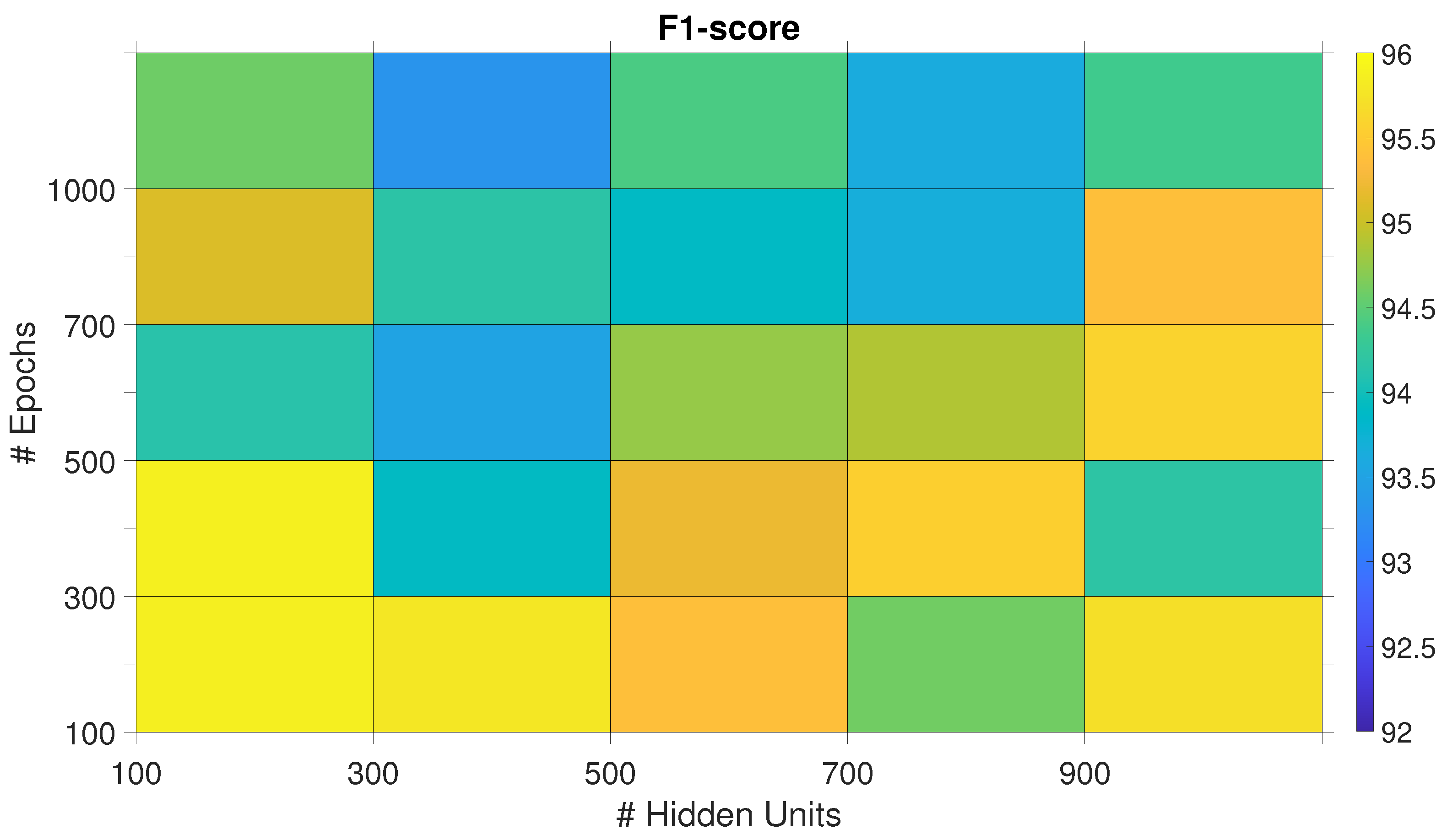
The performance of the network architectures obtained with the different Eps-HUs pairs are reported as checkerboard plots in Figure 2, Figure 3, and Figure 5, where colors are associated to F1-score. This visualization eases the observation of the best-performing parameters in terms of F1-score and how moving from these values deteriorates the network scores.
4.1.1. BiLSTM
The BiLSTM network classification performance converges to the maximum with 300 HUs and different values of Eps (Figure 2). The best Eps-HUs pair is 300HUs - 2500Eps with %, followed by 300HUs - 2000Eps and 300HUs - 1000Eps with %.
4.1.2. Sp-DAE
In Section 3.2.2, we introduced a large number of combinations of Eps-HUs pairs for the Sp-DAE. For the sake of clarity, we report only the subset of parameters that performed better, excluding combinations that provided limited F1-scores (Figure 3).
The Sp-DAE shows a stronger convergence in the middle of the checkerboard plot area. The best Eps-HUs pair is 2000HUs - 5500Eps with %, followed by 1100HUs - 5500Eps and 2000HUs - 5000Eps with %. Although the hyperparameters of Sp-DAE are strongly higher than BiLSTM, the loss of one percentage point of the F1-score compared to the BiLSTM suggests that the Recurrent Sp-DAE could improve the classification performance.
4.1.3. Recurrent Sp-DAE
As reported in Section 3.2.3, we trained 48 combinations of Sp-DAE and BiLSTM. Figure 4 shows the checkerboard plot of the F1-scores obtained and the Sp-DAE with 1300 HUs and 3500 Eps showed to be the best in extracting input features for BiLSTM. The best BiLSTM has 300 HUs and 2500 Eps followed by 4000 and 4500 Eps. All these Recurrent Sp-DAE have F1-scores close to %. Differently from SP-DAE, where the softmax layer better recognizes the different activities with features extracted by encoders with higher dimensions, in the Recurrent Sp-DAE, the features extracted by an encoder with smaller Eps and HUs perform better.
4.1.4. RCNN
Figure 5 shows the F1-scores of the RCNN trained with the proposed Eps-HUs pairs. Differently from the BiLSTM and the Sp-DAE networks, the RCNN exhibits higher classification performances with lower HUs and Eps keeping the F1-scores at the same level of the BiLSTM network. The best Eps-HUs pair is 100HUs - 300Eps with %, followed by 100HUs - 100Eps with %, and 300HUs - 100Eps with %.
Figure 5.
F1-score of the RCNN trained with different Eps-HUs pairs. The best-performing combinations are marked with black diamonds.
Figure 5.
F1-score of the RCNN trained with different Eps-HUs pairs. The best-performing combinations are marked with black diamonds.
4.2. Network architectures comparison
Training outcomes of the four different neural networks show that the Sp-DAE underperforms compared to the other two network architectures, regardless of the BiLSTM layers. Sp-DAEs are indeed stuck at an F1-score of more than one percentage less than the other architectures. Therefore, BiLSTM (%) and RCNN (%) are preferred to recognize MMH activities exploiting wearable sensors’ data and are further analyzed.
Figure 6 shows the F1-scores of these networks with the best three Eps-HUs pairs while varying the number of subjects in the training dataset. Dotted lines represent the overall average of F1-score. Regarding the BiLSTM, all the three hyperparameters pairs show great recognizing performances and, since the network complexity does not change, we decided to use the 300 HUs - 2500 Eps pair for the LOSO comparison (Section 4.3) since it has higher F1-score when trained with 14 subjects. In addition, the trend of the average F1-score shows a convergence to 95% with increasing subject numerosity and does not drop under the 95% threshold from the 11th subject. The RCNNs show almost the same overall means (%). Thus, we used the 100 HUs - 300 Eps pair for the LOSO comparison (Section 4.3), since it has a lower complexity and higher F1-score when trained with 14 subjects. In this case, the average F1-score shows a slightly increasing trend with increasing subject numbers.
4.3. Performance of the selected networks with LOSO validation
In the LOSO validation, we considered the BiLSTM with 300HUs-2500Eps and the RCNN with 100HUs-300Eps trained with subject numerosity ranging from 1 to 13. Figure 7 reports the F1-scores obtained for the two network architectures. Both show a convergent trend, but the maximum value, reached with 13 subjects, is % for the BiLSTM, while the RCNN stopped one percentage point below (%).
The F1-scores for each activity class obtained in the LOSO validation, considering 13 subjects in the training dataset, are reported (Table 4). The score is higher than or close to 90% for each class, except for the PT actions.
4.4. Comparison of the selected networks with SoA
Table 5 reports the F1-score, the MAC, and the MA operations of the BiLSTM with 300HUs-2500Eps and the RCNN with 100HUs-300Eps and the DeepConvLSTM with 128HUs as reported by Ordóñez and Roggen [21] and 300Eps as our RCNN. The network classification performances are reported for the split of the complete dataset and for the LOSO validation.
5. Discussion
Results presented in Section 4 show that BiLSTM and RCNN perform better than networks based on autoencoders, though being simpler in terms of parameters and epochs needed to achieve peak performance. In fact, the Sp-DAE, even if stacked with the BiLSTM architecture, reported the worst classification performances and they achieved higher scores only increasing the HUs number up to 2000. Surprisingly, adding the BiLSTM deteriorated the algorithm performance compared to softmax, suggesting that the extracted features canceled the potential benefits of time recursion.
In the training, BiLSTM and RCNN performed similarly, but RCNN showed an increasing trend of F1-score as the number of subjects in the dataset increased, suggesting that it could result in higher classification performances with more subjects. However, the addition of convolutional layers notably increases the network complexity compared to the BiLSTM. Also in the LOSO analysis, these networks performed similarly. However, the BiLSTM achieved a slightly better F1 score though being simpler than RCNN. Therefore, for this dataset, BiLSTM proved to be the best choice both in terms of classification performance maximization and optimization of the network complexity. However, the RCNN F1-score is close to BiLSTM’s, and it shows a slightly increasing trend of F1-score with the subject number, which makes it potentially perform better than BiLSTM. The potential improvement might justify the bigger complexity of the network and the consequent computational burden, but this trend should be confirmed and evaluated with a larger dataset.
The LOSO validation confirmed that both BiLSTM and RCNN have the potential to achieve high F1-scores when data comes from a new subject increasing the reasons to further investigate in this direction. This result is consistent with a similar BiLSTM architecture that has been implemented in [28] to classify MMH tasks. The authors obtained comparable F1-scores (91%) to ours but at the cost of using the FB configuration, composed of the 3-axis accelerations and angular velocities of all the 17 IMUs of the Xsens suit, resulting in 102 network inputs. This makes their network more complex and the method less flexible and generalizable since the users are forced to wear an FB suit equipped with IMUs to have suitable motion data. Conversely, the proposed BiLSTM network is much lighter, as the input is composed of only 10 variables. Moreover, using joint angles, velocity, and acceleration data opens the way to test and enhance the network with motion data gathered with other technologies such as RGB camera-based motion capture. This is a crucial point for HAR because the purchase and use of a FB suit can be unaffordable in MMH activities. Indeed, nowadays, many researchers exploit signals acquired with IMUs embedded in smartphones or even smartwatches for HAR of ADLs [49] and even MMH activities [50], but still with low classification performances.
The proposed RCNN is, to the best of our knowledge, a novel proposal for HAR, as the existing RCNN is much more complex. DeepConvLSTM [21] has four convolutional layers instead of our two layers and uses two LSTM layers instead of one GRU. The comparison with our proposed networks showed that DeepConvLSTM has similar (even lower) recognition performance despite its consistently higher computational cost. This may be intepreted with an unnecessary complexity of this network in relation to the classification task. This is confirmed by the application of this network in other datasets [22,50,51]. Considering the supposed target applications, the classification performance achieved on most classes allows using the proposed network. The most critical class was PT (placing the object on the table), which is mainly confused with the N-pose static position, maybe for its little variation of joint flexions especially when handling light loads (Figure 8). In the evaluation of the biomechanical overload due to MMH, which causes WMSDs, newly developed methods rely more and more on quantitative data instead of visual inspection of videos [52,53]. Both the proposed HAR networks enable automatic segmentation, thus drastically reducing the time that the rater needs for manual segmentation. However, if higher recognition performances are desired, the raters can review the network output and correct it, providing valuable new data to train the network and increase its classification ability.
6. Conclusion
This work has been motivated by the scarcity of research on HAR systems for MMH activities given its potential impact on the automatization of ergonomic risk assessment and human-robot collaboration in shared tasks. In this study, we compared different DL algorithms to classify MMH tasks and proposed the BiLSTM and the RCNN as the best choices. In fact, they achieve a similar (even better) classification performance with regards to the SoA with a significantly lower complexity. BiLSTM is preferable for network complexity, whereas RCNN should be taken into consideration for larger datasets. These networks require a limited set of motion and sEMG data and can be used in ecological settings in both logistics and industry. The abstraction from raw data encourages us to test these networks with motion data gathered with depth/stereo cameras, which would limit the number of wearable sensors and improve the feasibility of its pervasive use in MMH activities performed in spatially limited workplaces. Moreover, we plan to reduce the network input to minimize the sensors that the user needs to wear to obtain segmentation with comparable F1-score, thus enlarging possible applications of the proposed networks.
Author Contributions
Conceptualization, Giulia Bassani and Alessandro Filippeschi; Data curation, Giulia Bassani; Formal analysis, Alessandro Filippeschi; Funding acquisition, Carlo Alberto Avizzano and Alessandro Filippeschi; Investigation, Giulia Bassani; Methodology, Giulia Bassani and Alessandro Filippeschi; Resources, Carlo Alberto Avizzano; Software, Giulia Bassani; Supervision, Carlo Alberto Avizzano and Alessandro Filippeschi; Validation, Giulia Bassani and Alessandro Filippeschi; Visualization, Carlo Alberto Avizzano; Writing – original draft, Giulia Bassani; Writing – review & editing, Carlo Alberto Avizzano and Alessandro Filippeschi.
Funding
”The purchase of the devices used in this work was supported by the BRIEF “Biorobotics Research and Innovation Engineering Facilities” project (Project identification code IR0000036) funded under the National Recovery and Resilience Plan (NRRP), Mission 4 Component 2 Investment 3.1 of the Italian Ministry of University and Research funded by the European Union – NextGenerationEU.”
References
- Singh, D.; Merdivan, E.; Psychoula, I.; Kropf, J.; Hanke, S.; Geist, M.; Holzinger, A. Human activity recognition using recurrent neural networks. In Proceedings of the CD-MAKE. Springer; 2017; pp. 267–274. [Google Scholar]
- Schrader, L.; Toro, A.V.; Konietzny, S.; Rüping, S.; Schäpers, B.; Steinböck, M.; Krewer, C.; Müller, F.; Güttler, J.; Bock, T. Advanced sensing and human activity recognition in early intervention and rehabilitation of elderly people. Journal of Population Ageing 2020, 13, 139–165. [Google Scholar] [CrossRef]
- Malaisé, A.; Maurice, P.; Colas, F.; Ivaldi, S. Activity recognition for ergonomics assessment of industrial tasks with automatic feature selection. RA-L 2019, 4, 1132–1139. [Google Scholar] [CrossRef]
- Martínez-Villaseñor, L.; Ponce, H. A concise review on sensor signal acquisition and transformation applied to human activity recognition and human–robot interaction. IJDSN 2019, 15, 1550147719853987. [Google Scholar] [CrossRef]
- Azizi, S.; Yazdi, P.G.; Humairi, A.A.; Alsami, M.; Rashdi, B.A.; Zakwani, Z.A.; Sheikaili, S.A. Design and fabrication of intelligent material handling system in modern manufacturing with industry 4.0 approaches. IRATJ 2018, 4, 1–10. [Google Scholar] [CrossRef]
- Conforti, I.; Mileti, I.; Prete, Z.D.; Palermo, E. Measuring biomechanical risk in lifting load tasks through wearable system and machine-learning approach. Sensors 2020, 20, 1557. [Google Scholar] [CrossRef]
- Rajesh, R. Manual material handling: A classification scheme. Procedia Technology 2016, 24, 568–575. [Google Scholar] [CrossRef]
- Chen, K.; Zhang, D.; Yao, L.; Guo, B.; Yu, Z.; Liu, Y. Deep learning for sensor-based human activity recognition: Overview, challenges, and opportunities. CSUR 2021, 54, 1–40. [Google Scholar] [CrossRef]
- Nweke, H.F.; Teh, Y.W.; Al-Garadi, M.A.; Alo, U.R. Deep learning algorithms for human activity recognition using mobile and wearable sensor networks: State of the art and research challenges. Expert Systems with Applications 2018, 105, 233–261. [Google Scholar] [CrossRef]
- Luzheng, B.; Genetu, F.A.; Cuntai, G. A review on EMG-based motor intention prediction of continuous human upper limb motion for human-robot collaboration. Biomedical Signal Processing and Control 2019, 51, 113–127. [Google Scholar]
- Shin, S.; Baek, Y.; Lee, J.; Eun, Y.; Son, S.H. Korean sign language recognition using EMG and IMU sensors based on group-dependent NN models. In Proceedings of the SSCI. IEEE; 2017; pp. 1–7. [Google Scholar]
- Totah, D.; Ojeda, L.; Johnson, D.; Gates, D.; Provost, E.M.; Barton, K. Low-back electromyography (EMG) data-driven load classification for dynamic lifting tasks. PloS one 2018, 13, e0192938. [Google Scholar] [CrossRef]
- Attal, F.; Mohammed, S.; Dedabrishvili, M.; Chamroukhi, F.; Oukhellou, L.; Amirat, Y. Physical human activity recognition using wearable sensors. Sensors 2015, 15, 31314–31338. [Google Scholar] [CrossRef]
- Bulling, A.; Blanke, U.; Schiele, B. A tutorial on human activity recognition using body-worn inertial sensors. CSUR 2014, 46, 1–33. [Google Scholar] [CrossRef]
- Wang, J.; Chen, Y.; Hao, S.; Peng, X.; Hu, L. Deep learning for sensor-based activity recognition: A survey. Pattern recognition letters 2019, 119, 3–11. [Google Scholar] [CrossRef]
- Dentamaro, V.; Gattulli, V.; Impedovo, D.; Manca, F. Human activity recognition with smartphone-integrated sensors: A survey. Expert Systems with Applications 2024, 246, 123143. [Google Scholar] [CrossRef]
- Benmessabih, T.; Slama, R.; Havard, V.; Baudry, D. Online human motion analysis in industrial context: A review. Engineering Applications of Artificial Intelligence 2024, 131, 107850. [Google Scholar] [CrossRef]
- Trkov, M.; Stevenson, D.T.; Merryweather, A.S. Classifying hazardous movements and loads during manual materials handling using accelerometers and instrumented insoles. Applied ergonomics 2022, 101, 103693. [Google Scholar] [CrossRef] [PubMed]
- Syed, A.S.; Syed, Z.S.; Shah, M.; Saddar, S. Using wearable sensors for human activity recognition in logistics: A comparison of different feature sets and machine learning algorithms. IJACSA 2020, 11. [Google Scholar] [CrossRef]
- Bassani, G.; Filippeschi, A.; Avizzano, C.A. A Dataset of Human Motion and Muscular Activities in Manual Material Handling Tasks for Biomechanical and Ergonomic Analyses. Sensors Journal 2021, 21, 24731–24739. [Google Scholar] [CrossRef]
- Ordóñez, F.J.; Roggen, D. Deep convolutional and lstm recurrent neural networks for multimodal wearable activity recognition. Sensors 2016, 16, 115. [Google Scholar] [CrossRef]
- Yoshimura, N.; Morales, J.; Maekawa, T.; Hara, T. Openpack: A large-scale dataset for recognizing packaging works in iot-enabled logistic environments. In Proceedings of the PerCom. IEEE; 2024; pp. 90–97. [Google Scholar]
- Hochreiter, S. The vanishing gradient problem during learning recurrent neural nets and problem solutions. IJUFKS 1998, 6, 107–116. [Google Scholar] [CrossRef]
- Cho, K.; van Merrienboer, B.; Gulcehre, C.; Bahdanau, D.; Bougares, F.; Schwenk, H.; Bengio, Y. Learning phrase representations using RNN encoder-decoder for statistical machine translation. arXiv 2014, arXiv:1406.1078. [Google Scholar] [CrossRef]
- Greff, K.; Srivastava, R.K.; Koutník, J.; Steunebrink, B.; Schmidhuber, J. LSTM: A search space odyssey. IEEE transactions on neural networks and learning systems 2016, 28, 2222–2232. [Google Scholar] [CrossRef]
- Schuster, M.; Paliwal, K.K. Bidirectional recurrent neural networks. IEEE transactions on Signal Processing 1997, 45, 2673–2681. [Google Scholar] [CrossRef]
- Murad, A.; Pyun, J. Deep recurrent neural networks for human activity recognition. Sensors 2017, 17, 2556. [Google Scholar] [CrossRef] [PubMed]
- Porta, M.; Kim, S.; Pau, M.; Nussbaum, M.A. Classifying diverse manual material handling tasks using a single wearable sensor. Applied Ergonomics 2021, 93, 103386. [Google Scholar] [CrossRef]
- Arab, A.; Schmidt, A.; Aufderheide, D. Human Activity Recognition Using Sensor Fusion and Deep Learning for Ergonomics in Logistics Applications. In Proceedings of the IoTaIS. IEEE; 2023; pp. 254–260. [Google Scholar]
- Wang, L. Recognition of human activities using continuous autoencoders with wearable sensors. Sensors 2016, 16, 189. [Google Scholar] [CrossRef] [PubMed]
- Almaslukh, B.; AlMuhtadi, J.; Artoli, A. An effective deep autoencoder approach for online smartphone-based human activity recognition. IJCSNS 2017, 17, 160–165. [Google Scholar]
- Vincent, P.; Larochelle, H.; Bengio, Y.; Manzagol, P.A. Extracting and composing robust features with denoising autoencoders. In Proceedings of the ICML; 2008; pp. 1096–1103. [Google Scholar]
- Gu, F.; Khoshelham, K.; Valaee, S.; Shang, J.; Zhang, R. Locomotion activity recognition using stacked denoising autoencoders. IEEE Internet of Things Journal 2018, 5, 2085–2093. [Google Scholar] [CrossRef]
- Islam, M.M.; Nooruddin, S.; Karray, F.; Muhammad, G. Human activity recognition using tools of convolutional neural networks: A state of the art review, data sets, challenges, and future prospects. Computers in biology and medicine 2022, 149, 106060. [Google Scholar] [CrossRef]
- Niemann, F.; Lüdtke, S.; Bartelt, C.; Hompel, M.T. Context-aware human activity recognition in industrial processes. Sensors 2021, 22, 134. [Google Scholar] [CrossRef]
- Syed, A.S.; Syed, Z.S.; Memon, A.K. Continuous human activity recognition in logistics from inertial sensor data using temporal convolutions in CNN. IJACSA 2020, 11. [Google Scholar] [CrossRef]
- Xia, K.; Huang, J.; Wang, H. LSTM-CNN architecture for human activity recognition. Access 2020, 8, 56855–56866. [Google Scholar] [CrossRef]
- He, J.L.; Wang, J.H.; Lo, C.M.; Jiang, Z. Human Activity Recognition via Attention-Augmented TCN-BiGRU Fusion. Sensors 2025, 25, 5765. [Google Scholar] [CrossRef]
- Gao, X.; Luo, H.; Wang, Q.; Zhao, F.; Ye, L.; Zhang, Y. A human activity recognition algorithm based on stacking denoising autoencoder and lightGBM. Sensors 2019, 19, 947. [Google Scholar] [CrossRef]
- Li, Y.; Shi, D.; Ding, B.; Liu, D. Unsupervised feature learning for human activity recognition using smartphone sensors. In Proceedings of the MIKE. Springer; 2014; pp. 99–107. [Google Scholar]
- Bassani, G.; Filippeschi, A.; Avizzano, C.A. A wearable device to assist the evaluation of workers health based on inertial and sEMG signals. In Proceedings of the MED. IEEE; 2021; pp. 669–674. [Google Scholar]
- Losey, D.P.; McDonald, C.G.; Battaglia, E.; O’Malley, M.K. A review of intent detection, arbitration, and communication aspects of shared control for physical human–robot interaction. AMR 2018, 70, 010804. [Google Scholar] [CrossRef]
- Zhang, S.; Li, Y.; Zhang, S.; Shahabi, F.; Xia, S.; Deng, Y.; Alshurafa, N. Deep learning in human activity recognition with wearable sensors: A review on advances. Sensors 2022, 22, 1476. [Google Scholar] [CrossRef] [PubMed]
- Guan, Y.; Plötz, T. Ensembles of deep lstm learners for activity recognition using wearables. IMWUT 2017, 1, 1–28. [Google Scholar] [CrossRef]
- Buda, M.; Maki, A.; Mazurowski, M.A. A systematic study of the class imbalance problem in convolutional neural networks. Neural Networks 2018, 106, 249–259. [Google Scholar] [CrossRef]
- Krizhevsky, A.; Sutskever, I.; Hinton, G. Imagenet classification with deep convolutional neural networks. NeurIPS 2012, 25. [Google Scholar] [CrossRef]
- Grzeszick, R.; Lenk, J.M.; Rueda, F.M.; Fink, G.A.; Feldhorst, S.; Hompel, M.T. Deep neural network based human activity recognition for the order picking process. In Proceedings of the iWOAR; 2017; pp. 1–6. [Google Scholar]
- Freire, P.; Srivallapanondh, S.; Spinnler, B.; Napoli, A.; Costa, N.; Prilepsky, J.E.; Turitsyn, S.K. Computational complexity optimization of neural network-based equalizers in digital signal processing: a comprehensive approach. JLT 2024. [Google Scholar] [CrossRef]
- Huang, J.; Lin, S.; Wang, N.; Dai, G.; Xie, Y.; Zhou, J. TSE-CNN: A two-stage end-to-end CNN for human activity recognition. JBHI 2019, 24, 292–299. [Google Scholar] [CrossRef] [PubMed]
- Morales, J.; Yoshimura, N.; Xia, Q.; Wada, A.; Namioka, Y.; Maekawa, T. Acceleration-based human activity recognition of packaging tasks using motif-guided attention networks. In Proceedings of the PerCom. IEEE; 2022; pp. 1–12. [Google Scholar]
- Kuschan, J.; Filaretov, H.; Krüger, J. Inertial measurement unit based human action recognition dataset for cyclic overhead car assembly and disassembly. In Proceedings of the INDIN. IEEE; 2022; pp. 469–476. [Google Scholar]
- Giannini, P.; Bassani, G.; Avizzano, C.A.; Filippeschi, A. Wearable sensor network for biomechanical overload assessment in manual material handling. Sensors 2020, 20, 3877. [Google Scholar] [CrossRef] [PubMed]
- Stefana, E.; Marciano, F.; Rossi, D.; Cocca, P.; Tomasoni, G. Wearable devices for ergonomics: A systematic literature review. Sensors 2021, 21, 777. [Google Scholar] [CrossRef] [PubMed]
Figure 1.
The graphical representation of the network architectures: (a) BiLSTM; ((b)) Sp-DAE; ((c)) Recurrent Sp-DAE; ((d)) RCNN.
Figure 1.
The graphical representation of the network architectures: (a) BiLSTM; ((b)) Sp-DAE; ((c)) Recurrent Sp-DAE; ((d)) RCNN.
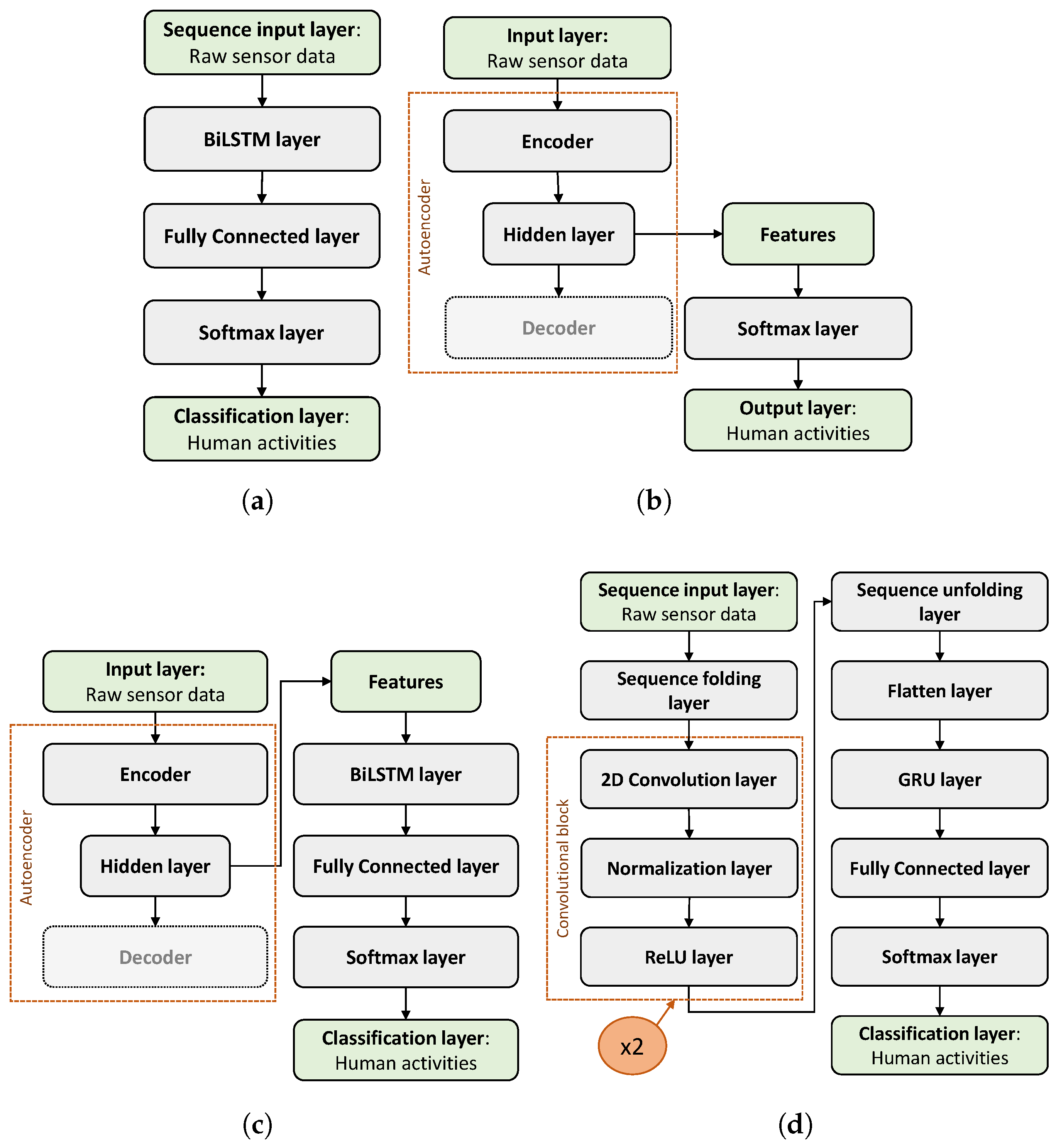
Figure 2.
F1-score of the BiLSTM netoworks trained with different Eps - HUs pairs. Selected pairs are marked with black diamonds.
Figure 2.
F1-score of the BiLSTM netoworks trained with different Eps - HUs pairs. Selected pairs are marked with black diamonds.
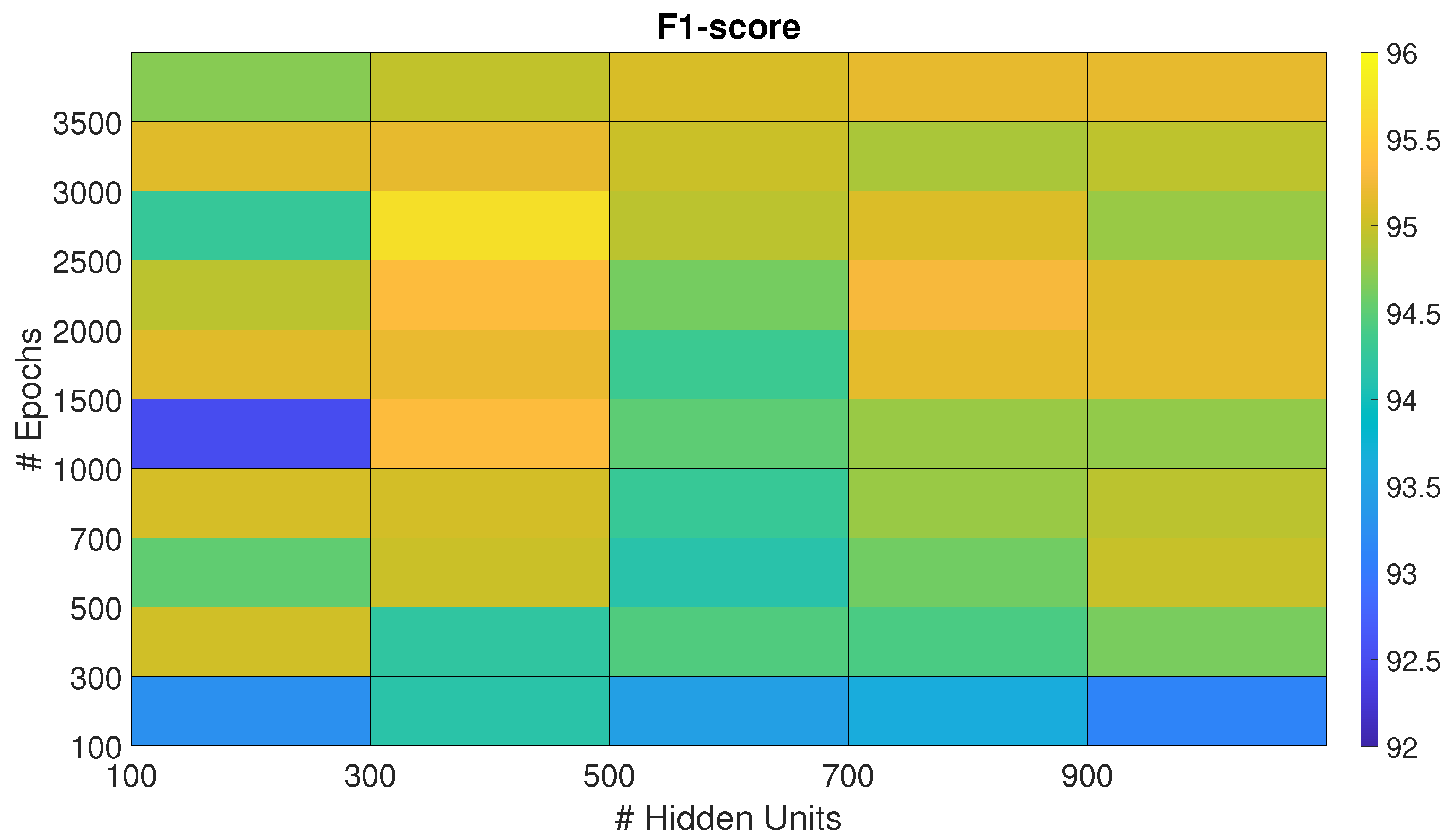
Figure 3.
F1-score of the Sp-DAE trained with different Eps-HUs pairs. Selected pairs are marked with black diamonds.
Figure 3.
F1-score of the Sp-DAE trained with different Eps-HUs pairs. Selected pairs are marked with black diamonds.
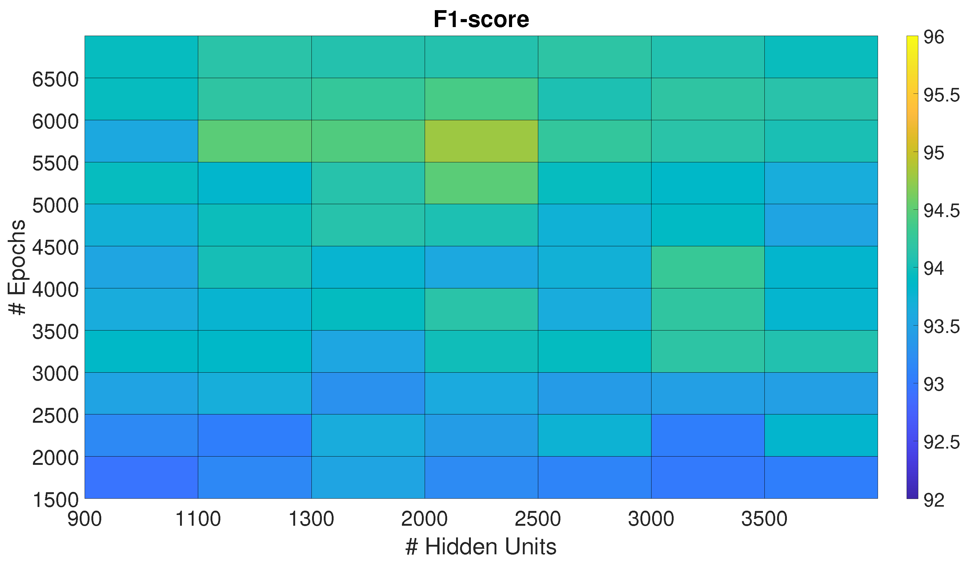
Figure 4.
F1-score of the Recurrent Sp-DAE trained with different Sp-DAE-BiLSTM combinations. The best-performing combination is marked with a black diamond.
Figure 4.
F1-score of the Recurrent Sp-DAE trained with different Sp-DAE-BiLSTM combinations. The best-performing combination is marked with a black diamond.
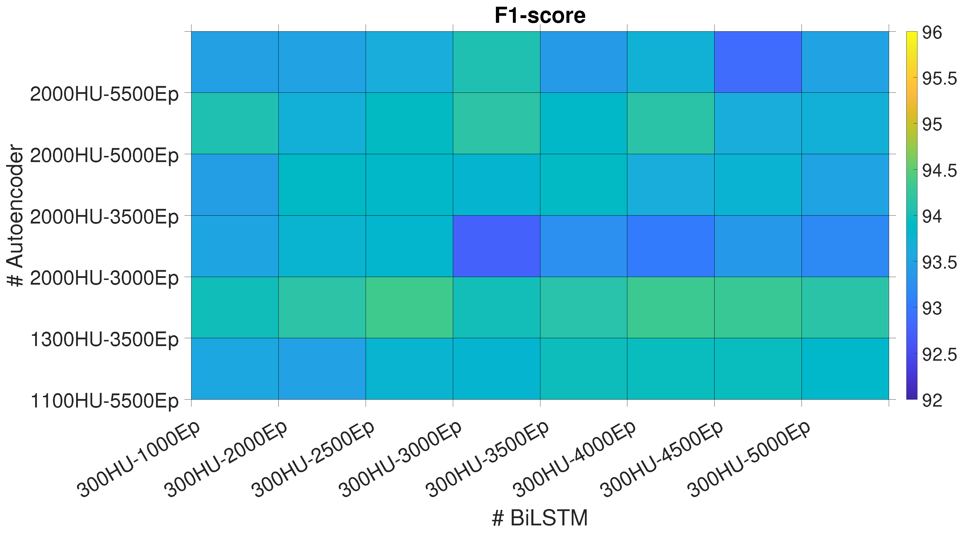
Figure 6.
F1-score for each subject numerosities of the different architectures with the best epochs number - hidden units pairs.
Figure 6.
F1-score for each subject numerosities of the different architectures with the best epochs number - hidden units pairs.
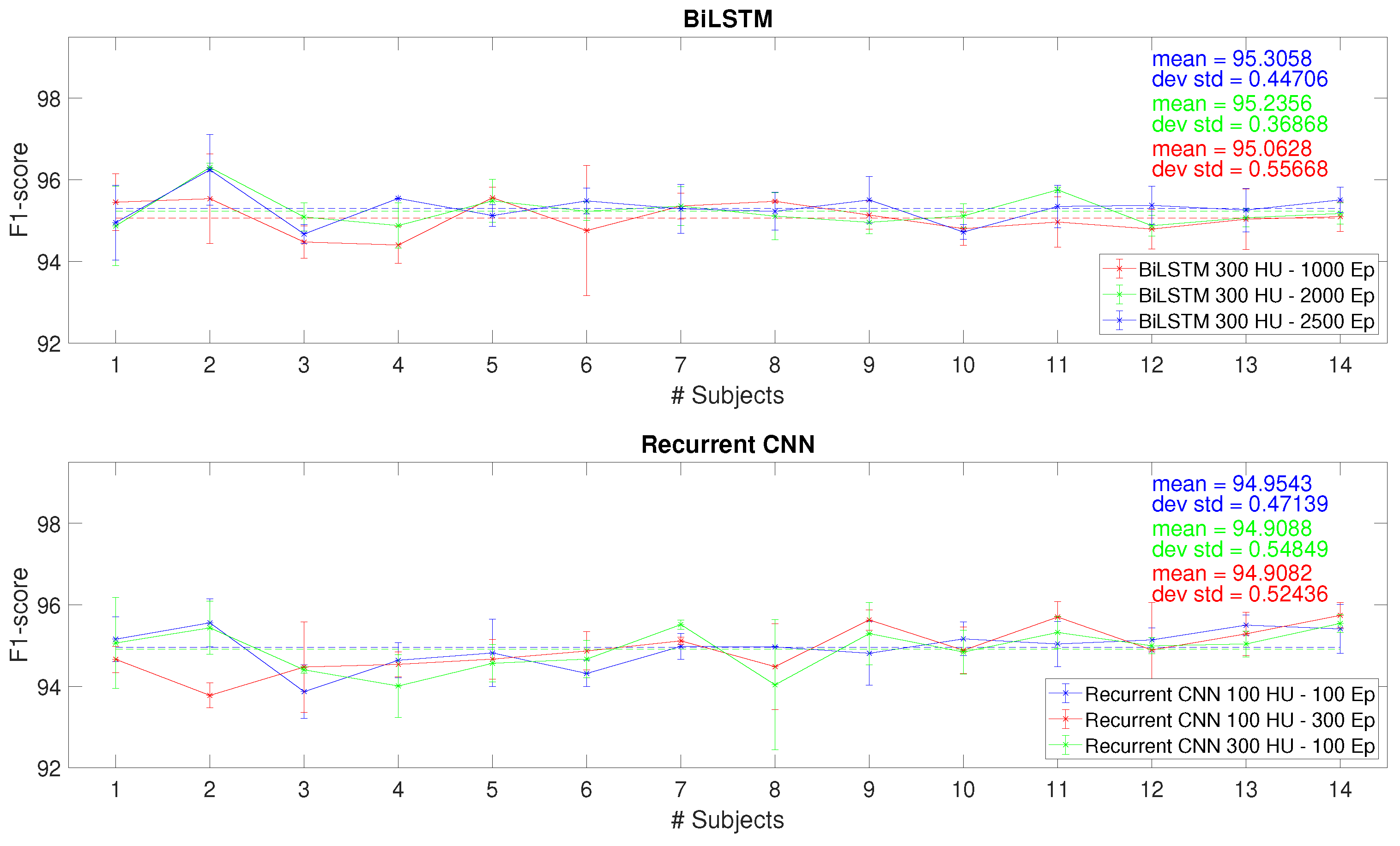
Figure 7.
F1-score for each subject numerosities with the LOSO test of the (a) BiLSTM with 300 HUs and 2500 Eps and (b) RCNN with 100 HUs and 300 Eps.
Figure 7.
F1-score for each subject numerosities with the LOSO test of the (a) BiLSTM with 300 HUs and 2500 Eps and (b) RCNN with 100 HUs and 300 Eps.
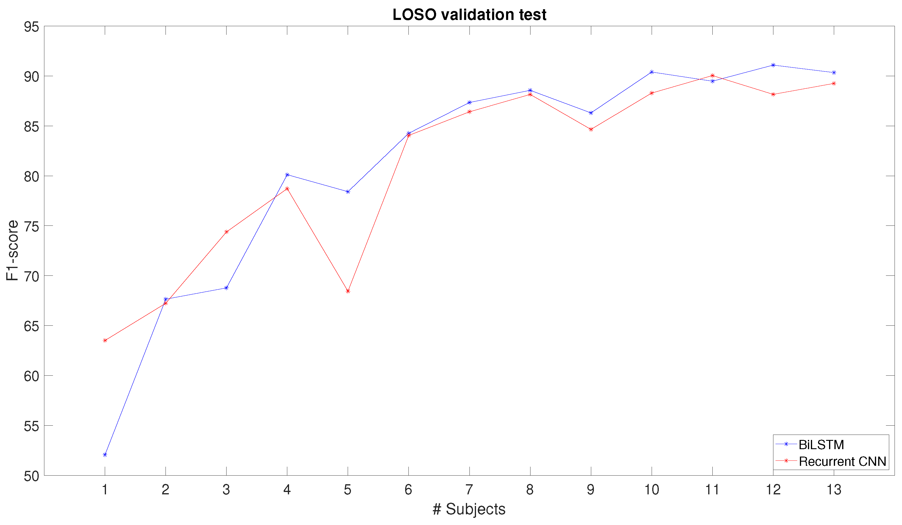
Figure 8.
Confusion matrices of the test data for the BiLSTM and RCNN network architectures.
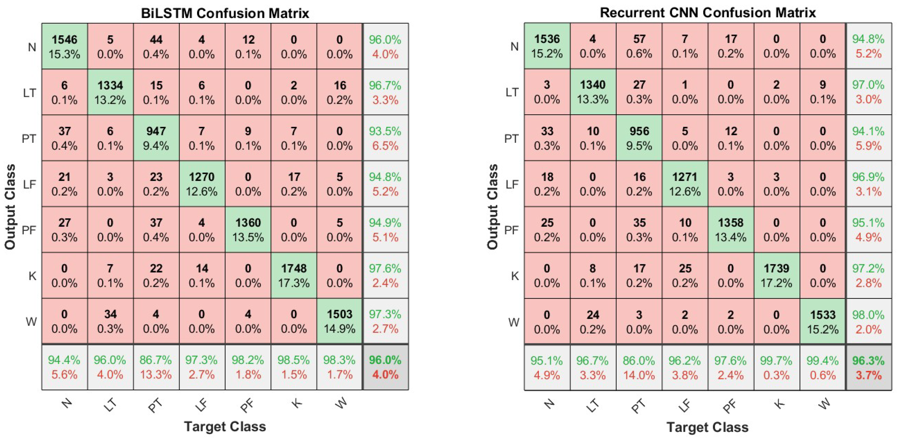

Table 1.
Hyperparameters used in the BiLSTM trainings.
| Hyperparameter | Value |
|---|---|
| Input size | 10 |
| Optimizer | Adam |
| Maximum epochs | 100, 300, 500, 700, 1000, 1500, 2000, 2500, 3000, 3500 |
| Hidden units | 100, 300, 500, 700, 900 |
| Batch size | 128 |
| Initial Learning rate | |
| Learning rate drop factor | |
| Learning rate drop period | 10 |
| L2 regularization | |
| Loss function | Cross-entropy loss |
Table 2.
Hyperparameters used in the SpDAE trainings.
| Hyperparameter | Value |
|---|---|
| Input size | 10 |
| Maximum epochs | 100, 300, 500, 700, 1000, 1300, 1500, 2000, 2500, 3000, 3500, 4000, 4500, 5000, 5500, 6000, 6500 |
| Hidden units | 100, 300, 500, 700, 900, 1100, 1300, 2000, 2500, 3000, 3500 |
| Training algorithm | Conjugate gradient descent |
| Sparsity Regularization | 1 |
| Sparsity proportion | |
| L2 regularization | |
| Transfer function | log-sigmoid |
| Loss function | Sparse mse |
Table 3.
Values of hyperparameters used in the RCNN trainings.
| Hyperparameter | Value |
|---|---|
| Input size | 10x240 |
| Filter size | 3x3 |
| Filter dimension | 32 |
| Padding | 0 |
| 1° CNN layer stride | 1x1 |
| 2° CNN layer stride | 1x4 |
| 1° CNN layer dilation factor | 1x1 |
| 2° CNN layer dilation factor | 2x2 |
| Maximum epochs | 100, 300, 500, 700, 1000 |
| Hidden units | 100, 300, 500, 700, 900 |
Table 4.
F1-score for each action.
| Action | BiLSTM | RCNN |
|---|---|---|
| N-pose (N) | 89.1% | 90.1% |
| Lifting from the Table (LT) | 94.5% | 92.4% |
| Placing on the Table (PT) | 84% | 85.1% |
| Lifting from the Floor (LF) | 90.3% | 88.7% |
| Placing on the Floor (PF) | 88.8% | 86.7% |
| Keeping lifted (K) | 92.3% | 91.4% |
| Carrying (W) | 93.4% | 90.2% |
Table 5.
Comparison among BiLSTM, RCNN, and DeepConvLSTM.
| Neural network | F1-score 70-30 split | F1-score LOSO | MAC | MA |
|---|---|---|---|---|
| BiLSTM | 95.7% | 90.3% | 1492200 | 1532400 |
| RCNN | 95.9% | 89.2% | 2724028 | 5448056 |
| DeepConvLSTM | 95.2% | 90.3% | 327027584 | 543762176 |
Disclaimer/Publisher’s Note: The statements, opinions and data contained in all publications are solely those of the individual author(s) and contributor(s) and not of MDPI and/or the editor(s). MDPI and/or the editor(s) disclaim responsibility for any injury to people or property resulting from any ideas, methods, instructions or products referred to in the content. |
© 2025 by the authors. Licensee MDPI, Basel, Switzerland. This article is an open access article distributed under the terms and conditions of the Creative Commons Attribution (CC BY) license (http://creativecommons.org/licenses/by/4.0/).
Copyright: This open access article is published under a Creative Commons CC BY 4.0 license, which permit the free download, distribution, and reuse, provided that the author and preprint are cited in any reuse.


