Submitted:
26 September 2025
Posted:
29 September 2025
You are already at the latest version
Abstract
A new method to estimate future samples in time series data is presented and it is compared against the well known technique ESPRIT. It exploits the null space of the Hankel matrix of the data allowing the prediction of future samples with better accuracy and confidence. In a more general sense the notion of null space refers to the set of eigenvectors of the data Hankel matrix which are associated with the smallest eigenvalues. The method is fully deterministic with comparable computational complexity to ESPRIT. Testing involves 4000 randomly chosen data sets with variable spectral characteristics.
Keywords:
Time-series
; forecast
; non-parametric
; optimization
; null-space
1. Introduction
Difference equations have been widely used to model time series by means of exponential functions. The parameters of the exponential functions result from an optimization process that minimizes the modelling error. These techniques suffer from numerical problems that affect the accuracy of the computed parameters. The frequencies and the dumping factors of the exponential functions are the roots of polynomials that result from the optimization process. However the numerical computation of roots is rather sensitive leading to compromised accuracy. To overcome this problem, alternative approaches for the computation of the exponential parameters were proposed in literature. Among the most efficient techniques are the well-known ESPRIT and HSVD algorithms that perform well when it comes to spectral estimation but continue having numerical problems to predict future samples [1,2]. In addition round-off errors add-up creating significant deviation from the correct values of the parameters which compromises the prediction based on extrapolation of the exponential functions.
2. Materials and Methods
2.1. The Orthogonal Approach
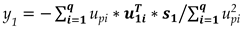
Let us consider the pth order Hankel matrix H of a given set x of N samples with N>p and size px(N-p+1). The SVD of H is H=U*S*V where U is a pxp matrix of singular vectors of size p, S is a pxp diagonal matrix of singular values, arranged in ascending order and V is a px(N-p+1) matrix of singular vectors of size (N-p+1) [3]. Assuming that the size of the null space of H is q only p-q singular values in S are non-zero and q of the singular vectors of U namely u1… uq span the null space of H. If Uq is a pxq matrix of these vectors then the N-p+1 vectors of H are orthogonal to Uq [4,5,6]. The (N+1)th unknown sample of the set x, namely x(N+1) along with the p-1 known samples x(N-p+2), x(N-p+3) … x(N) form a new vector of size p, namely x1 which is part of the augmented Hankel matrix Ha1=[H x1]. Since all the vectors of H are orthogonal to Uq the same should hold for the vectors of the augmented Ha1, hence x1 is also orthogonal to Uq. By splitting x1 into two parts, the known part namely =[x(N-p+2) x(N-p+3) … x(N)] and the unknown part y1=x(N+1) the following equation is obtained.
 Where u1i consists of the p-1 first components of the ith singular vector ui and upi is the last component of ui.
Equation (1) is only theoretically valid. In real life the orthogonality is only approximate and (1) should be reformulated as follows,
 where e1i is the approximation error. Best approximation will be achieved when the accumulated squared error is minimized,
 which leads to the solution of the following minimization problem,
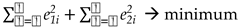
An equivalent minimization problem results after elaborating the above expression (3),

By setting to zero the first derivative of (4) with respect to y1 the following solution is obtained,
2.2. The Case of Two Unknown Samples
To estimate x(N+1) and x(N+2) simultaneously a similar approach is used. Besides the vector x1 a second vector x2 of size p, consisting of p-2 known samples x(N-p+3), x(N-p+4),.. x(N) and two unknown samples, namely x(N+1) and x(N+2) is formed. The augmented Hankel matrix Ha1 becomes Ha2=[H x1 x2] and both vectors x1 and x2 have to be orthogonal to Uq. Consequently next to equation (1) an additional equation to guarantee the orthogonality of x2 is needed. Vector x2 is split into two parts, the known part s2 and the unknown components y1 and y2 with =[x(N-p+3) x(N-p+4 … x(N)] and [y1 y2]=[x(N+1) x(N+2)]. Due to the orthogonality property the following must hold,
 where u2i consists of the p-2 first components of the ith singular vector ui and up-1,i and upi are the last two components of ui.
As it was mentioned before, equation (6) is only theoretically valid. In real life the orthogonality is only approximate and (6) should be reformulated as follows,
 where e2i is the approximation error. For best estimates of both x(N+1) and x(N+2) the following combined optimization problem must be solved,
By using (1.1) and (7) the above minimization problem can be expressed as,

To solve the above the first derivatives of expression (9) with respect to y1 and y2 are set to zero. This leads to the following two equations,


The above linear system of equations provides best estimates for y1 and y2.
2.3. The General Case of Many Unknown Samples
When three future samples need to be estimated, a third term in the optimization problem (8) is added [7]. By following the same type of notation equation (8) becomes,
 where e3i is the error due to the third unknown sample x(N+3)=y3
By following the same notation as in the case of two unknown samples the error e3i can be expressed as follows,
 where =[x(N-p+4) x(N-p+4 … x(N)] , u3i consists of the p-3 first components of the ith singular vector ui and up-2,i , up-1,i and upi are the last three components of ui.
By setting the first derivatives of expression (11) with respect to y1, y2 and y3 to zero, a linear system of three equations is formed and its solution provides the estimates of the three unknown samples y1, y2 and y3 .
By replacing (1), (7) and (12) into expression (11) and by elaborating on the algebraic manipulations, the following set of equations is obtained,
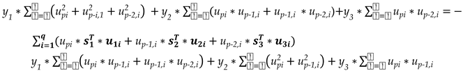


The above system of equations (13) maybe expressed as,
 where y=[y1 y2 y3], A is a symmetric matrix and b is a vector.
In a more general notation, the elements of the symmetric matrix A for all j ≤ k and k≤n can be expressed as,
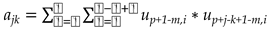 where n stands for the number of samples to be estimated, namely n=3 in this case.
Similarly, the elements of b can be expressed as,
With A and b known, the estimation of y is straightforward based on equation (14),
 where y is the vector of n unknown future samples of the set x.
3. Results
The proposed algorithm was tested against the well known method ESPRIT that models the signal by means of exponential sinusoids. A large set of signals, four thousands in total, with variable complexity in terms of the rank of their covariance matrix was considered. The comparison was based on the accuracy of predicting future samples as well as on the overall consistency of the two algorithms. The term consistency refers to the homogeneity of the prediction errors. Each signal consists of 2000 to 2500 samples and it was generated from white noise that was filtered using random low pass FIR filters with hundreds of taps. Four sets of future samples were selected for the comparison. The latter is based on the RMSE among the predicted values and the actual values of the signals. The four sets refer to predicting the first, tenth, twentieth and thirtieth future samples using both the proposed and the ESPRIT algorithms and comparing the RMSEs of the two methods. To evaluate the algorithms with respect to their consistency the variance of the errors is used. In order to eliminate variations due to the differences of the signal amplitudes, all errors were normalized with respect to the actual value of the predicted sample.
For the ESPRIT method the prediction for each one of the 4000 signals is based on twenty different models with orders equally spaced between 140 and 900. By averaging these twenty different results the overall prediction is computed.
For the new method the size p of the Hankel matrix H is set to 600. Alternative choices for p were also tested showing no significant change in the results as long as p is not too small compared to the length N of the signals. Regarding the null space not only one single size for each signal is used. Instead, an optimum set of null spaces for each signal is considered and the overall prediction is computed by averaging individual results. There are two constraints while choosing the optimum set of null spaces, a) the sizes of the null spaces of the optimum set are consecutive numbers and b) the variance of the results of the set is minimal. The second constraint is imposed to guarantee maximum consistency of the chosen set.
Table 1 shows the obtained results for the four different setups in predicting future samples. In all cases the new method performs better than ESPRIT in terms of both RMSE and variance.
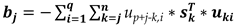
Figure 1, Figure 2, Figure 3 and Figure 4 show the shape of representative signals among the 4000 used. The rank of the covariance matrix of all 4000 signals varies considerably, ranging from low to high rank. This way the results are not biased with respect to the degree of predictability of the signals.
4. Discussion
A new method to predict future samples is presented and it is compared against the ESPRIT method. The new method was proven to be more accurate and more consistent than ESPRIT, based on results from four thousand time series of variable spectral complexity. The new method exploits the properties of the eigenvectors of the Hankel matrix of the time series that are associated with the low eigenvalues. It is fast and stable and can predict any set of future samples. Further research will focus on both the selection of the null space of the time series Hankel matrix and the choice of the matrix size.
References
- S. van Huffel, H. Chen, C. Decanniere and P. van Hecke, "Algorithm for time-domain NMR data fitting based on total least squares", J.Magn.Res., Series A 110, pp. 228-237, 1994. [CrossRef]
- Roy R., Paulraj A., and Kailath T., “ESPRIT—a subspace rotation approach to estimation of parameters of cisoids in noise”, IEEE Transactions on Acoustics, Speech, and Signal Processing. (1986) 34, no. 5, 1340–1342, 2-s2.0-0022794413. [CrossRef]
- R.A. Horn, C.R. Johnson, “Matrix Analysis”, Cambridge University Press, 1996.
- I.Dologlou and G.Carayannis, "LPC/SVD analysis of signals with zero modelling error", Signal Processing, Vol. 23 (3), pp. 293-298, 1991. [CrossRef]
- I. Dologlou, G. Carayannis, "Physical interpretation of signal reconstruction from reduced rank matrices", IEEE Trans. Acoust. Speech Signal Process., ASSP, July 1991, pp. 1681-1682. [CrossRef]
- J.A. Cadzow, "Signal enhancement: A composite property mapping algorithm", IEEE Trans. Acoust. Speech Signal Process., Vol. 36, No. 1, January 1998, pp. 49-62. [CrossRef]
- Ioannis Dologlou, “Estimating future samples in time series data”. July 2025. [CrossRef]
Figure 1.
Typical signal among the 4000 used (high rank covariance).
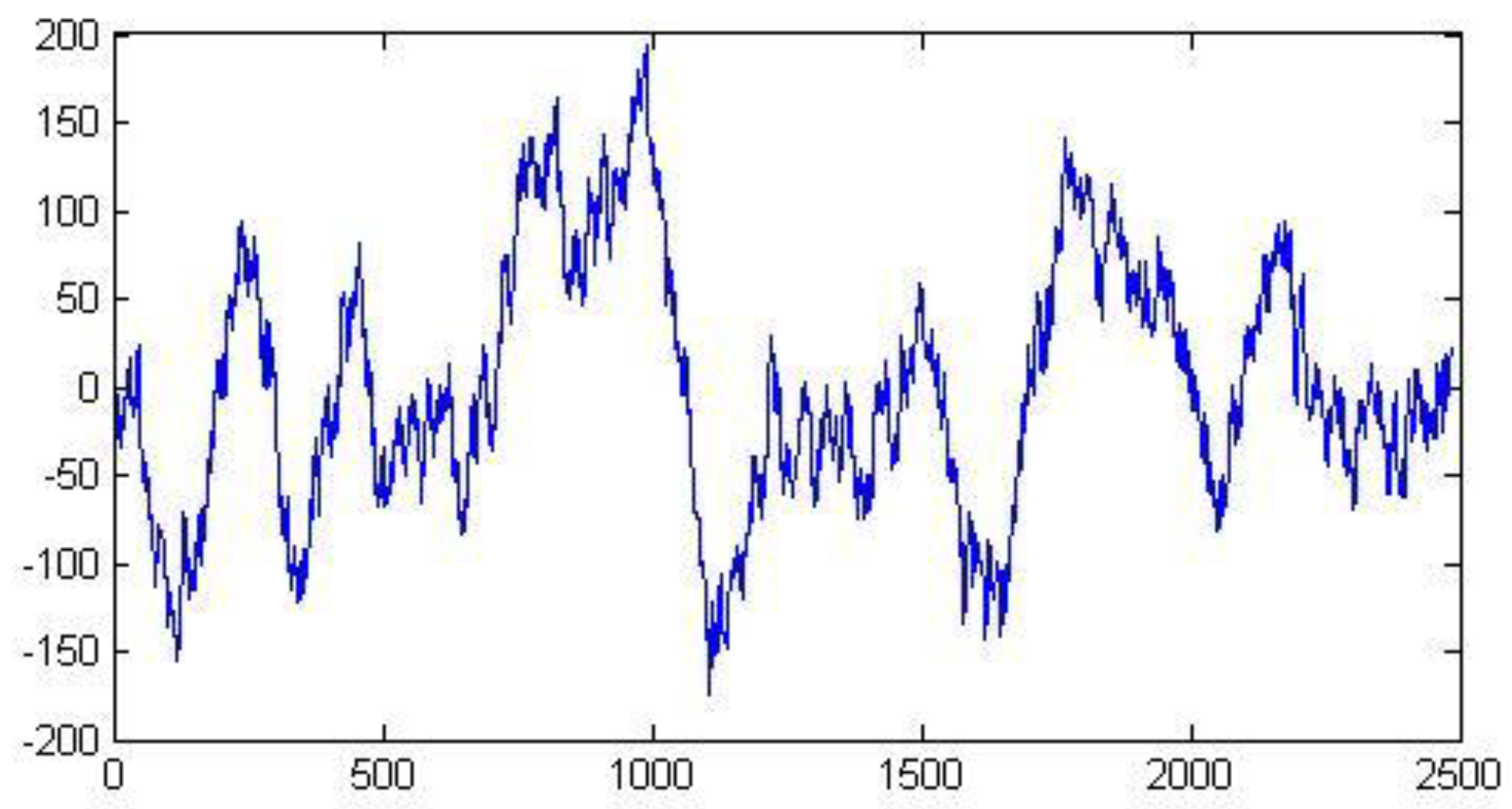
Figure 2.
Typical signal among the 4000 used (high rank covariance).
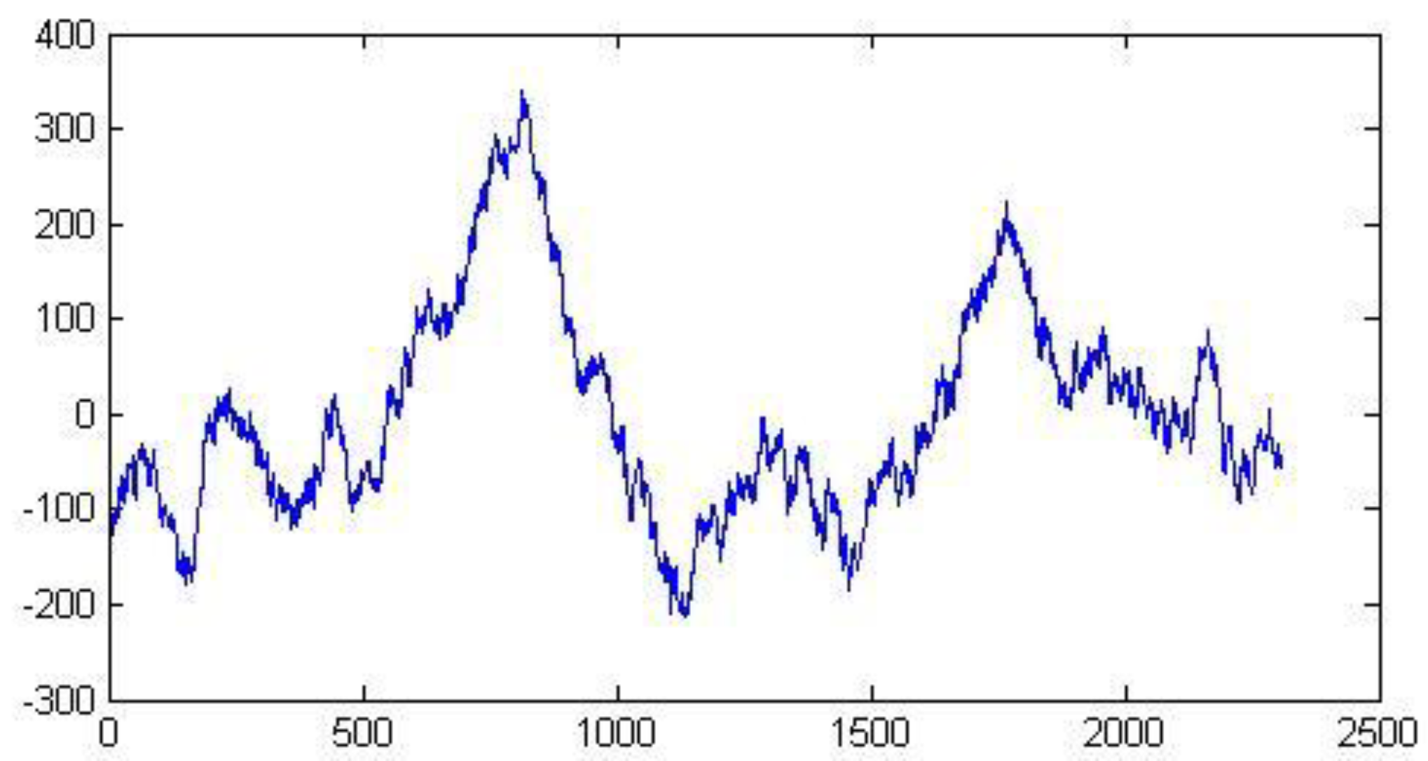
Figure 3.
Typical signal among the 4000 used (low rank covariance).
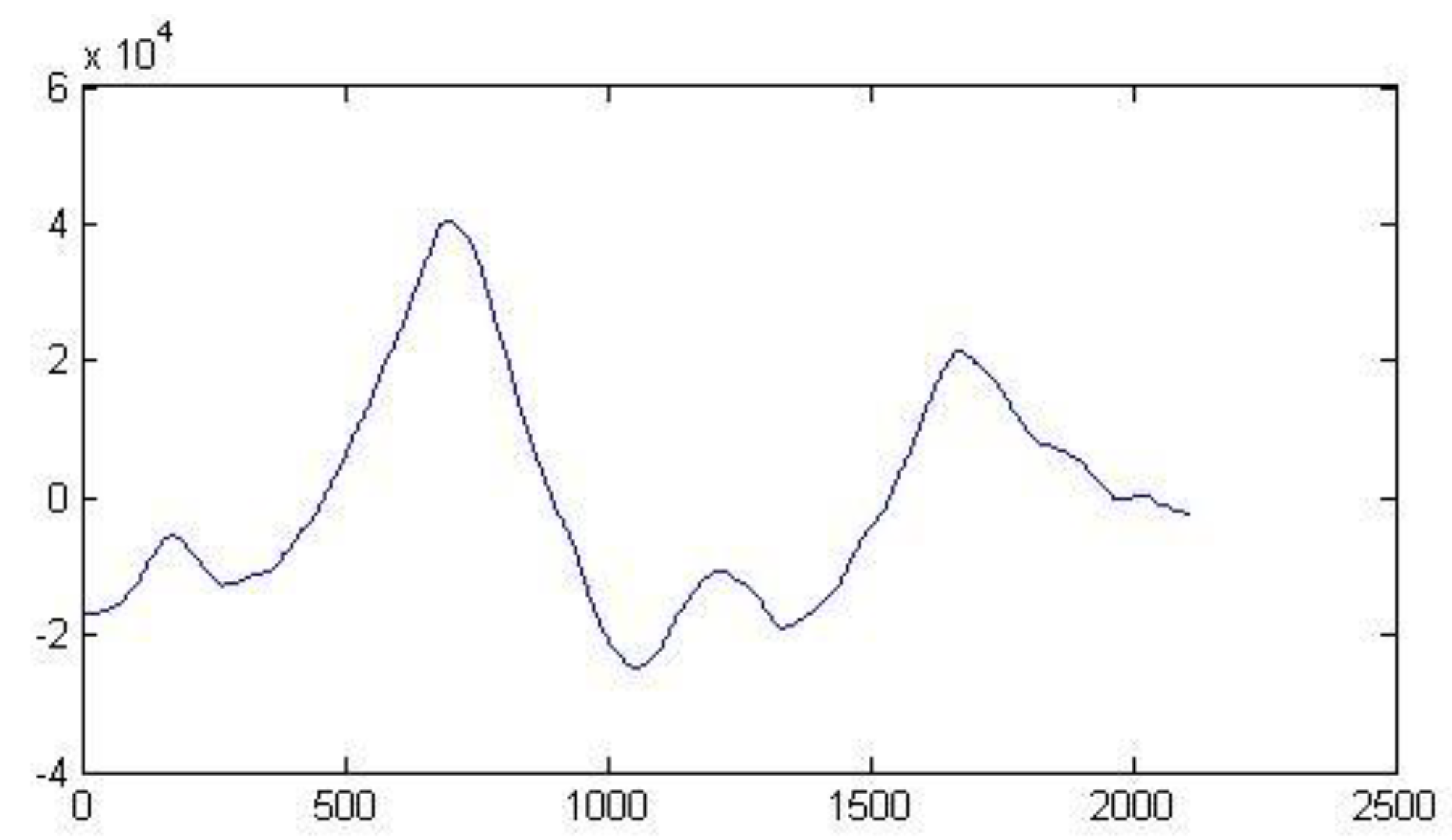
Figure 4.
Typical signal among the 4000 used (low rank covariance).
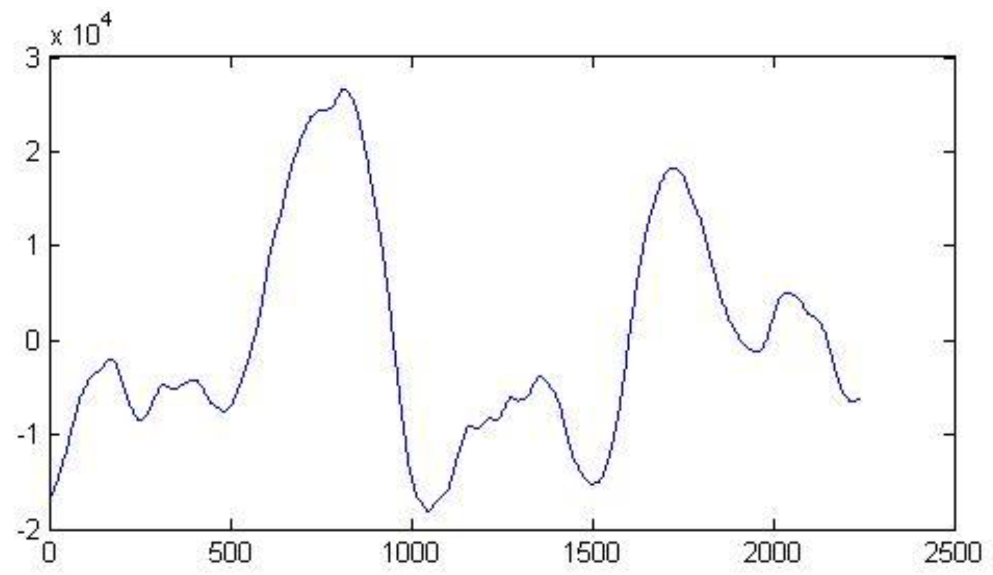

Table 1.
RMSE and variance for the same set of 4000 signals using the new method and ESPRIT. Results refer to the estimation of the 1st, 10th, 20th, and 30th future samples.
Table 1.
RMSE and variance for the same set of 4000 signals using the new method and ESPRIT. Results refer to the estimation of the 1st, 10th, 20th, and 30th future samples.
| Number of tested signals | RMSE New Method |
Variance New Method | RMSE ESPRIT | Variance ESPRIT | |
| 1st Future sample | 4000 | 9.707*10-4 | 8.378*10-7 | 0.0052 | 2.65*10-5 |
| 10th Future sample | 4000 | 0.0064 | 4.0922*10-5 | 0.0737 | 0.0054 |
| 20th Future sample | 4000 | 0.0128 | 1.624*10-4 | 0.1933 | 0.0373 |
| 30th Future sample | 4000 | 0.0149 | 2.2255*10-4 | 0.4215 | 0.1777 |
Disclaimer/Publisher’s Note: The statements, opinions and data contained in all publications are solely those of the individual author(s) and contributor(s) and not of MDPI and/or the editor(s). MDPI and/or the editor(s) disclaim responsibility for any injury to people or property resulting from any ideas, methods, instructions or products referred to in the content. |
© 2025 by the authors. Licensee MDPI, Basel, Switzerland. This article is an open access article distributed under the terms and conditions of the Creative Commons Attribution (CC BY) license (http://creativecommons.org/licenses/by/4.0/).
Copyright: This open access article is published under a Creative Commons CC BY 4.0 license, which permit the free download, distribution, and reuse, provided that the author and preprint are cited in any reuse.


