Submitted:
22 September 2025
Posted:
25 September 2025
You are already at the latest version
Abstract
Spiking Neural Networks (SNNs) provide a biologically inspired, event-driven alternative to Artificial Neural Networks (ANNs) with the potential to deliver competitive accuracy at substantially lower energy. This tutorial-study offers a unified, practice-oriented assessment combining critical reviews and standardized experiments. We benchmark a shallow Fully Connected Network (FCN) on MNIST and a deeper VGG7 architecture on CIFAR-10 across multiple neuron models (leaky Integrate-and-Fire (LIF), Sigma-Delta, etc.) and input encodings (direct, rate, temporal, etc.) using supervised surrogate-gradient training, implemented with Intel Lava/SLAYER, SpikingJelly, Norse and PyTorch. Empirically, we observe a consistent but tunable trade-off between accuracy and energy. On MNIST, Sigma-Delta neurons with rate or Sigma-Delta encodings reach 98.1% (ANN: 98.23%). On CIFAR-10, Sigma-Delta neurons with direct input achieve 83.0% at just 2 time steps (ANN: 83.6%). A GPU-based operation-count energy proxy indicates many SNN configurations operate below the ANN energy baseline; some frugal codes minimize energy at the cost of accuracy, whereas accuracy-leaning settings (e.g., Sigma-Delta with direct or rate coding ) narrow the performance gap while remaining energy-conscious, yielding up to 3-fold efficiency versus matched ANNs in our setup. Thresholds and the number of time steps are decisive: intermediate thresholds and the minimal time window that still meets accuracy targets typically maximize efficiency per joule. We distill actionable design rules: choose the neuron/encoding pair by application goal (accuracy-critical vs. energy-constrained) and co-tune thresholds and time steps. Finally, we outline how event-driven neuromorphic hardware can amplify these savings through sparse, local, asynchronous computation, providing a practical playbook for embedded, real-time, and sustainable AI deployments.
Keywords:
Spiking Neural Networks
; Artificial Neural Networks
; Energy Efficiency
; Supervised Learning
; Implementation Guidelines
; Software Tools
1. Introduction
Modern AI systems—especially deep neural networks—have delivered impressive accuracy across vision, language, and control, but at rapidly growing computational and energy costs [1,2]. Mitigation strategies such as pruning and quantization reduce multiply–accumulate (MAC) counts and memory traffic [3,4,5]. Yet, the overall footprint of state-of-the-art models continues to raise sustainability concerns [6]. This tension motivates exploration of alternatives that are accurate and power-aware. Recent studies show conventional ML tackling embedded and industrial tasks under tight resource and latency constraints [7,8,9], underscoring the need for more event-driven, energy-efficient approaches.
Spiking neural networks (SNNs) offer a biologically inspired, event-driven paradigm in which information is conveyed by discrete spikes over time [10,11]. Their sparse, asynchronous computation and temporal coding can translate to lower energy on neuromorphic substrates, while naturally capturing temporal structure [12,13,14,15]. At the same time, practical deployment remains challenging: spikes are non-differentiable, complicating gradient-based optimization [16,17,18]; performance depends critically on the choice of encoding scheme [19,20]; and toolchains and benchmarks for fair SNN–ANN comparisons are still maturing.
Gap. The key gap lies in the lack of a unified, practice-oriented analysis: existing surveys often treat neuron models, encodings, learning rules, and software stacks in isolation, providing limited apples-to-apples evidence on accuracy–energy trade-offs against equivalent ANN baselines across both shallow and deep regimes. A comprehensive perspective that links design choices to measurable performance and power remains scarce.[18,19,20,21,22,23,24,25,26,27,28,29,30,31,32,33]
This work. We address this gap by combining a comprehensive, critical review with a hands-on tutorial and standardized benchmarking:
- We systematize SNN components: neuron models (Integrate-and-Fire (IF) / Leaky Integrate-and-Fire (LIF), Adaptive Leaky Integrate-and-Fire (ALIF), Exponential Integrate-and-Fire / Adaptive Exponential integrate-and-fire (EIF/AdEx), Resonate-and-Fire (RF), Hodgkin–Huxley (HH), Izhikevich, Resonate-and-Fire–Izhikevich hybrid (RF–Iz), Current-Based neuron (CUBA), Sigma–Delta ()), neural encodings (direct/single-value encoding, rate coding, temporal variants including Time-to-First-Spike (TTFS), Rank-Order with Number-of-Spikes (R–NoM), population coding, phase-of-firing coding (PoFC), burst coding, Sigma–Delta encoding ()), and learning paradigms(review scope): supervised ( backpropagation-through-time (BPTT) with surrogate gradients; e.g., SLAYER, SuperSpike, EventProp), unsupervised (spike-timing–dependent plasticity(STDP) and variants), reinforcement (reward-modulated (R-STDP), e-prop), hybrid supervised STDP (SSTDP), and ANN→SNN conversion. and Practical pipeline used here: supervised training via BPTT with surrogate gradients (aTan by default; SLAYER/SuperSpike-style updates) for the tutorial and benchmarks. [16,17,18,19].
- We provide a practical tutorial (with reference to a representative neuromorphic software stack, e.g., Lava) covering model construction, encoding choices, and training/inference workflows suitable for resource-constrained deployment.
- We establish a side-by-side evaluation protocol that compares SNNs with architecturally matched ANNs on a shallow setting (MNIST) and a deeper convolutional setting (CIFAR-10 with VGG-style backbones [34]). Metrics include task accuracy/timesteps, spike activity, and power-oriented proxies to illuminate accuracy–efficiency trade-offs.
- We distill design guidelines that map application goals—accuracy targets and per-inference energy budgets—onto actionable choices of neuron model, encoding scheme, number of time steps, and supervised surrogate-gradient training (e.g., SLAYER, SuperSpike, aTan).
Scope and structure.Section 2 reviews encoding strategies, covers neuron models, and outlines learning paradigms and training methods. Section 3 details the experimental setup, the evaluation protocol, and software setup; Section 4 presents comparative results on MNIST and CIFAR-10; Section 4.4 discusses implications; Section 5 concludes with recommendations and future directions. We aim to offer a coherent pathway from principles to practice, helping readers design SNNs that balance accuracy with energy efficiency in real-world settings.
Scope and structure.Section 2 reviews spiking neural network fundamentals, including encoding strategies, neuron models, and learning paradigms. Section 3 presents the datasets, experimental setup, model architectures, and software tools. Section 4 reports the comparative performance and energy analyses on MNIST and CIFAR-10, and provides an integrated discussion of accuracy–energy trade-offs and design implications. Finally, Section 5 summarizes key findings and offers recommendations for future research. Our aim is to provide a coherent pathway from principles to practice, guiding the design of SNNs that balance accuracy with energy efficiency in real-world deployments.
2. Background of Spiking Neural Networks
SNNs are widely regarded as the “third generation” of neural models, narrowing the gap between artificial neural networks (ANNs) and biological computation by representing information with discrete spike events over time [10,35]. Whereas ANNs operate with continuous activations and synchronous MAC operations [36], SNNs exploit sparse, event-driven accumulate updates. This temporal, asynchronous processing aligns with neural physiology and can yield substantial energy savings—particularly on neuromorphic hardware—while natively handling time-dependent signals.
2.0.0.1. Processing pipeline:
Figure 1 outlines a generic SNN workflow comprising encoding, network processing, decoding, and learning. In the encoding stage, external signals are transformed into spike trains. Common strategies include rate codes, time-based codes (e.g., TTFS or inter-spike intervals), and population codes, chosen according to signal statistics and latency/energy constraints. For instance, image intensities can be converted to Poisson spike trains whose rates are proportional to pixel values [37]. During network processing, spikes propagate through layers of model neurons—e.g., LIF, AdEx, Iz, or HH—whose subthreshold dynamics and thresholds shape temporal integration and spike generation [38,39]. Decoding then maps output spike activity to decisions, using spike counts (rate), precise timing (temporal), or pooled population activity, depending on task requirements [37]. Learning rules—supervised, unsupervised, reinforcement, or hybrids—adjust synapses to meet behavioral goals.
2.0.0.2. Power efficiency: mechanisms and practice:
SNN efficiency stems from sparsity (computation occurs only on spike events), lower-cost AC updates in place of dense MACs, and event-driven memory traffic that reduces data movement—often the dominant energy term in modern systems [40,41]. On neuromorphic substrates (e.g., Intel Loihi neuromorphic processor, IBM TrueNorth, SpiNNaker), these properties translate into significant system-level gains via fine-grained parallelism, on-chip routing of spikes, and local memory near compute [42,43,44,45,46,47]. Empirically, energy per inference scales with the total number of synaptic events and the average firing rate; thus design knobs—encoding sparsity (e.g., TTFS, ), neuron/leaky constants, thresholds, rate regularizers, and time-window length—directly trade accuracy for energy [28,37,48]. Comparative studies report multi× efficiency improvements for SNNs in event-rich settings and on dedicated hardware [42,45,49], while highlighting the importance of maintaining low spike rates and co-optimizing algorithms with hardware constraints.
2.0.0.3. Advantages and challenges:
By construction, SNNs capture temporal dependencies with high timing resolution. They can compute efficiently in sparse regimes, enabling low-latency, low-power inference in settings such as event-based sensing and edge computing [25,28,48]. However, three obstacles temper widespread adoption. First, spike non-differentiability complicates gradient-based training; practical solutions rely on surrogate gradients, exact adjoints, local plasticity, or ANN-to-SNN conversion, each with trade-offs in accuracy, stability, or hardware fit [16,17,18]. Second, performance can lag ANN baselines if encoders/decoders and neuron models are not co-designed with the task [50]. Third, software and hardware ecosystems are still maturing, and standardized, energy-aware benchmarks remain limited.
2.0.0.4. Learning and encoding:
Unsupervised learning often uses spike-timing–dependent plasticity (STDP) to uncover structure from temporal correlations [51]. Supervised training employs BPTT with surrogate gradients to approximate spike derivatives, enabling deep SNN optimization [16]. Reinforcement learning modulates synaptic changes via reward signals, supporting closed-loop control and robotics [52]. Encoding choices strongly influence latency and energy: rate codes are robust but can be spike-heavy; time-based codes reduce spikes and latency but demand precise timing; population codes improve separability and noise tolerance at added computational cost.
2.0.0.5. Real-world applications:
SNNs have been validated across domains where temporal precision and energy constraints dominate. In event-based vision, SNNs on neuromorphic hardware achieve real-time gesture recognition on Dynamic Vision Sensor Gesture with milliwatt-scale budgets [42,53],
robust object/gesture processing on mobile platforms [54,55], and low-latency tracking/control [56,57]. Beyond human-centric vision, embedded deep models are used for animal affect recognition [9]; here SNNs offer a path to lower-latency, lower-power inference for on-animal or field-deployed sensors.
In robotics and closed-loop control,while conventional ANN-based controllers remain prevalent in practice [58,59] spike-based policies run on-chip for responsive, power-aware navigation and manipulation [53,56]. In biomedical signal processing, SNNs support wearable ECG/EEG analytics and brain–computer interfaces with stringent energy and latency requirements [60,61,62,63].
In industrial monitoring and tribology, neural models estimate lubrication parameters from sensor data [7], a setting where spike-based, event-driven inference could reduce power and latency at the edge.
For time-series forecasting, SNNs model nonstationary environmental and energy signals, with conventional ML baselines in subsurface/energy operations providing context for accuracy–efficiency comparisons [8] (e.g., wind/solar) while keeping inference costs low [64,65,66,67,68]. In finance and IoT/edge analytics, event-driven SNNs process sparse, asynchronous streams for anomaly detection and prediction under tight power budgets [69,70,71,72]. These deployments underscore SNNs’ capacity to convert biological inspiration into practical, energy-efficient intelligence—particularly when learning rules, encoding schemes, and neuron models are co-designed with the target hardware and workload.
2.1. Encoding in SNNs
Encoding is a pivotal process in SNNs, transforming continuous-valued inputs into discrete spike events and thereby bridging the gap between external stimuli and spike-based information processing [73]. This transformation is central to leveraging the distinctive advantages of SNNs, including temporal dynamics, event-driven computation, and energy efficiency [74]. The choice of encoding strategy directly affects how effectively information is represented, how temporal patterns are captured, and how power-efficiently the network operates—properties that are crucial for real-time processing and deployment on neuromorphic hardware [75].
Despite their importance, encoding schemes face several design challenges. These include balancing representational accuracy with computational complexity, maintaining biological plausibility, and ensuring compatibility with neuromorphic circuits [76,77]. Furthermore, encoding decisions strongly influence system robustness, as some strategies offer greater resilience to noise or adversarial perturbations than others [78]. As a result, encoding research has increasingly focused on systematically exploring and optimizing strategies to enhance scalability and efficiency, thereby positioning SNNs as viable alternatives to traditional ANNs in energy-constrained and real-time environments [79].
This subsection reviews the main categories of encoding schemes used in SNNs, emphasizing their respective strengths and limitations. Table 1 provides a comparative overview, while Figure 2 and Figure 3 illustrate representative examples. The first figure highlights three fundamental approaches—rate, TTFS, and burst coding—while the second figure expands the view to include inter-spike interval, N-of-M, population, and PoFC coding. Together, these visualizations and the summary table provide an integrated perspective on the diverse ways in which information can be encoded in SNNs.
2.1.1. Rate Coding
Rate coding represents stimulus intensity by the number of spikes emitted within a time window,
Its simplicity, biological plausibility, and the clean correspondence between firing rates and ANN activations make it a common choice for image/signal processing and embedded deployments where robustness and implementation ease are priorities [78]. Because it averages over a window T, however, it discards fine timing. It often requires longer windows or higher spike counts to reach accuracy—raising latency and energy—so it is less suited to rapid, event-driven scenarios [78,80].
2.1.2. Direct Input Encoding
Direct input encoding feeds continuous-valued signals (e.g., pixel intensities) directly to the input layer without synthesizing spikes [74,78]. By bypassing stochastic spike generation, it can cut timesteps and improve latency and accuracy—useful for deep architectures and large-scale vision or real-time decision tasks—while preserving input fidelity and simplifying the front end [76]. This convenience, however, forgoes event-driven sparsity: multi-bit input activity increases compute and energy versus spike-based schemes and reduces biological plausibility, making it a weaker fit for resource- or power-constrained neuromorphic deployments [73,74,78,81].
2.1.3. Temporal Coding
Temporal coding emphasizes the precise timing of spikes rather than their average rate, aligning with biological evidence that timing carries rich and rapidly accessible information [24,38,75]. By leveraging when spikes occur, this family of methods offers faster and potentially more energy-efficient information transfer compared to rate coding. Several variants exist:
- Time-to-First-Spike (TTFS): encodes stimulus strength in the latency of the first spike:where is stimulus onset and the delay before firing [14]. TTFS is highly power-efficient, as minimal spiking activity can support rapid decisions, though it requires precise timing and complicates learning.
- Inter-Spike Interval (ISI): uses the time gap between consecutive spikes,providing richer temporal detail at the cost of increased spiking and energy use [14].
- N-of-M (NoM) Coding: transmits only the first N of M possible spikes, enhancing hardware efficiency but discarding spike-order information [82].
- Rank Order Coding (ROC): exploits the sequence of spike arrivals according to synaptic weights, offering high discriminability but at the cost of computational intensity and sensitivity to precise timing [24].
- Ranked-N-of-M (R-NoM): integrates ROC and NoM by propagating the first N spikes while weighting their order:where is a decreasing modulation with spike order [82].
Critically, temporal coding can yield more information per spike and support low-latency decisions, potentially reducing total energy if efficiently implemented. Yet, it introduces challenges in robustness: decoding is complex, schemes are sensitive to noise and spike-timing variability, and training deep SNNs with precise temporal codes remains difficult [76]. These trade-offs highlight temporal coding as a powerful but demanding alternative, most suitable when rapid responses and acceptable temporal resolution outweigh simplicity and energy stability.
2.1.4. Population Coding
Population coding distributes information over an ensemble, improving robustness and separability—useful for noisy, time-varying signals (e.g., speech/audio, sensor fusion)—but at the cost of more neurons, decoding overhead, and energy/memory traffic [83,84]. A common readout is the weighted population response.
with neuron weights and responses ; this complements latency/phase-based schemes by pooling precise temporal cues while trading efficiency for reliability [83,84].
2.1.5. Encoding
encoding transmits changes rather than absolute values via a simple feedback loop,
where is the input, the increment, the emitted spike, and an accumulated reconstruction error. Focusing on differences yields sparse spike trains with strong temporal fidelity and lower energy, suiting dynamic, streaming signals on neuromorphic and wearable/biomedical platforms [74,78]. Noise–shaping aids robust reconstruction [85,86,87], though effective deployment requires careful threshold/feedback tuning and circuit-aware trade-offs between fidelity, latency, and power [88].
2.1.6. Burst Coding
Burst coding represents information with short, high-frequency spike packets—mirroring rhythmic patterns observed in cortex and subcortex [13,75,89,90]. A burst for neuron i over a window can be written as
where indicates a spike at time t. Packing spikes in brief episodes supports rapid information transfer and strong temporal cues with fewer decision windows, which is attractive for event-rich sensing and closed-loop control; at the same time, coordinating burst onset and network-wide timing complicates decoding and hardware scaling, and poorly tuned burst parameters can negate energy savings [13,75,89,90]. In practice, burst coding is most useful when biological realism and efficient processing of temporally complex signals are priorities, provided synchronization and parameterization are carefully managed.
2.1.7. PoFC Coding
PoFC encodes information by the phase of each spike relative to an ongoing oscillation (e.g., theta/gamma) [87,91,92,93]. The phase of the i-th spike is
with the oscillation reference and its period. By leveraging phase locking observed in hippocampus and other circuits, PoFC can pack more information per spike than rate codes—enabling rich, low-count representations and potentially lower energy—yet it relies on precise synchronization and is sensitive to timing jitter; accurate phase extraction and integration with plasticity (e.g., STDP) add implementation complexity [91,92,93]. PoFC is most compelling for high-fidelity temporal discrimination and navigation/sensory tasks shaped by oscillatory dynamics, while resource-constrained neuromorphic deployments must balance its representational gains against robustness and hardware simplicity [87].
2.1.8. Impact of Encoding Schemes on SNN Performance and Power Efficiency
Encoding is a primary lever for both representation and compute/energy footprint. Foundational work spans modulation for efficient analog–to–spike conversion [85] and temporally rich schemes like rank–order coding [24]; subsequent surveys emphasize that the “best” code is application-dependent, balancing accuracy, latency, energy, robustness, and hardware constraints [73]. Recent refinements show (i) interfaces adapted to SNNs preserve fidelity over wide dynamics while cutting spikes, at the cost of feedback tuning and circuit complexity [86,87]; (ii) unified analyses of TTFS/ROC/NoM/R–NoM clarify discriminability under realistic noise and timing variability, and differentiable training narrows the gap to gradient-based optimization [76,82]; and (iii) hybrid/dynamic schemes (e.g., layer-wise burst+phase or attention-gated temporal codes) improve throughput-per-watt without sacrificing accuracy [13,94,95]. Comparative trends remain consistent: direct-input (analog) encoding lowers timesteps and can boost accuracy/latency on deep tasks but forgoes event-driven sparsity at the input stage [74]; rate coding is simple, conversion-friendly, and relatively robust yet loses fine timing and may need longer windows or higher spike counts [78]; temporal codes (TTFS/ISI) offer high information per spike and fast decisions but are jitter-sensitive and harder to train/deserialize at scale [14,82]; population coding strengthens separability and noise tolerance for temporally rich signals at the expense of neuron count and decoding cost [84]. Table 1 and Figure 2, Figure 3, and Figure 4 summarize these trade-offs.
2.1.8.1. Guidelines for Selecting an Encoding Scheme.
2.2. SNN Neuron Models
Neuron models are the computational primitives of SNNs: they determine how synaptic events are integrated, how spikes are generated, and how signals propagate through a network. Their choice governs representational power, energy consumption, latency, and hardware suitability [10,38,96]. Broadly, models lie on a spectrum that trades biological detail for computational efficiency. At one extreme, biophysical formulations such as HH accurately reproduce membrane dynamics but are expensive at scale [97,98]. Toward the efficient end, families of integrate-and-fire models (IF, LIF and extensions such as ALIF, QIF/EIF, SRM) abstract spiking as filtered integration plus thresholding, enabling large networks and low-power deployment [38]. Intermediate phenomenological models (Izhikevich, AdEx, RF) reproduce rich firing patterns with moderate cost, offering a pragmatic balance for many tasks [39,99].
Selecting a neuron model is therefore an application-driven decision that weighs fidelity, efficiency, and implementation complexity. Detailed conductance-based models can be advantageous for tasks requiring precise subthreshold or adaptation dynamics; simplified IF variants often suffice for rate-based processing and fast, energy-aware inference; intermediate models are attractive when diverse temporal patterns are essential but resources are limited. Additional considerations include the availability of stable learning rules (e.g., surrogate-gradient training for LIF/AdEx/Izhikevich), robustness to noise and device non-idealities, and the target hardware’s support for state variables and synaptic dynamics [96,98,99]. A concise, per-model synopsis of mechanisms, advantages, and challenges is provided in Table 2.
2.2.1. Spike Response Model (SRM)
The SRM is a compact, kernel-based description of a spiking neuron in which the membrane potential is the superposition of post-synaptic response kernels and a spike-triggered afterpotential [38,100]:
where is the last spike time, a refractory/after-spike kernel, a synaptic filter, and the input drive. Spikes occur when crosses a dynamic threshold,
with absolute refractory period and exponential recovery to . SRM spans fixed-kernel variants (SRM0) and versions with spike-triggered threshold adaptation/state-dependent kernels (SRM+), unifying integrate-and-fire dynamics while remaining analytically tractable and efficient for event-driven simulation. This separation of synaptic and refractory effects makes SRM convenient for modeling STDP, probing computational properties, and hardware-friendly implementations. Being phenomenological, however, it lacks rich subthreshold biophysics (e.g., voltage-gated conductances or resonance) unless extended, and practical use requires careful calibration of , , and [38].
2.2.2. Integrate-and-Fire (IF) and Leaky Integrate-and-Fire (LIF)
The integrate-and-fire family models a neuron as a linear integrator with threshold-and-reset dynamics [38,101,102,103,104]: when crosses from below, a spike is emitted and (optionally with a refractory period). Its minimal state, analytical tractability, and event-driven simulation make it a staple for large-scale SNNs and neuromorphic deployment.
2.2.2.1. Perfect IF (PIF).
An ideal, non-leaky integrator accumulates input without passive decay,
with capacitance C and input current . Once , a spike occurs and . PIF is computationally minimal but overestimates temporal integration by omitting leak.
2.2.2.2. Leaky IF (LIF).
illustarted in Figure 5 Incorporating passive leak yields
with , membrane resistance R, and resting potential . LIF captures membrane decay, supports stochastic analysis, and enables efficient event-driven updates [38,103].
IF/LIF deliver simplicity, stability, and compatibility with surrogate-gradient training, but their linear subthreshold dynamics lack conductance nonlinearities (e.g., adaptation, resonance). In practice they are often augmented (ALIF) or extended (EIF/AdEx) when richer temporal behavior is required.
2.2.3. Adaptive Leaky Integrate-and-Fire (ALIF)
ALIF augments LIF with spike-frequency adaptation, reproducing reduced firing under sustained drive via either a dynamic threshold or a spike-triggered hyperpolarizing current [38,100,105]. This adds history dependence while retaining efficient, event-driven simulation and surrogate-gradient trainability.
2.2.3.1. Dynamic-threshold ALIF.
where , is baseline threshold, adaptation strength, and its decay; on a spike at , .
2.2.3.2. Current-based ALIF.
with adaptation current , jump b per spike, and decay ; after a spike , .
2.2.4. Exponential Integrate-and-Fire (EIF)
The EIF neuron sharpens spike initiation by adding an exponential term to the leaky membrane dynamics, providing a smooth, biophysically motivated threshold [38,106]. In current-based form,
where is the resting potential, the rheobase (effective spike-initiation) voltage, the slope factor controlling the sharpness of onset, and the input current. A spike is emitted when diverges past a set peak (e.g., ), after which and an absolute refractory period may be imposed.
Compared with LIF, EIF reproduces the rapid upstroke of action potentials and more accurate responses to fast, fluctuating inputs (gain, phase response, and f–I curves) while remaining far cheaper than conductance-based models [104,106]. The extra nonlinearity and parameters improve fidelity but require calibration (notably and ) and can stiffen numerical integration near threshold. EIF serves as a practical compromise for studies of high-frequency synaptic integration, spike initiation, and neuromorphic implementations that need a smooth, differentiable surrogate of threshold dynamics [38].
2.2.5. Adaptive Exponential Integrate-and-Fire (AdEx)
AdEx extends LIF with an exponential spike-initiation term and a spike-triggered adaptation variable, yielding a compact neuron that reproduces regular-/fast-spiking, adapting, and bursting behaviors [107]:
where is membrane potential, capacitance, leak conductance, leak reversal, spike-initiation voltage, slope factor, w the adaptation current, a subthreshold adaptation, its time constant, and synaptic current. A spike is registered when exceeds , after which and (optional absolute refractory).
EIF-like sharp onset supports realistic spike initiation, while captures spike-frequency adaptation and bursting at modest cost, enabling efficient numerical integration and event-driven simulation. Hardware-oriented variants (fixed-point/high-accuracy arithmetic, power-of-two linearizations, CORDIC exponentials) further reduce runtime without sacrificing fidelity [108,109,110]. Careful calibration of , , and adaptation parameters is essential; near-threshold stiffness may require smaller steps or dedicated solvers. In practice, AdEx is a good default when richer dynamics than LIF are needed with only a slight complexity increase.
2.2.6. Resonate-and-Fire (RF)
The RF neuron captures subthreshold oscillations and frequency selectivity—complementing integrator-style IF/LIF models—via a complex state with linear dynamics [111]:
where encodes the oscillatory state, is the intrinsic angular frequency, sets damping (stability requires ), are synaptic couplings, and are pre-synaptic spike impulses at times . A spike is emitted when a readout (e.g., or a linear projection of ) crosses threshold from below, followed by a reset . Writing reveals a damped resonator with eigenvalues , producing natural selectivity to inputs near and to spike phase—useful for tasks rich in temporal structure, resonance, and phase-/PoFC-style coding.
In practice, RF offers lightweight oscillatory dynamics that simulate efficiently and admit analysis; balanced RF (BRF) improves stability in recurrent SNNs by regulating excitation–inhibition [112], and analog realizations demonstrate direct signal-to-spike conversion for edge sensing without explicit A/D front-ends [113]. As a phenomenological model, however, spiking is threshold-based (not biophysical), channel nonlinearities are implicit, parameters (frequency, damping, reset) require calibration, and the second-order state increases per-neuron cost versus IF/LIF; for strongly nonlinear spiking such as complex bursting, AdEx or Izhikevich variants can be preferable.
2.2.7. Hodgkin–Huxley (HH)
The HH model gives a biophysical account of spike generation via voltage–gated and channels plus leak, fit to voltage–clamp data from squid axon [97]. The membrane equation balances capacitive and ionic currents:
with gating kinetics
As the gold standard for single–cell fidelity, HH reproduces subthreshold dynamics, spike upstroke, refractoriness, and pharmacological effects, making it ideal for mechanism studies and validating reduced models. Its computational cost (stiff ODEs, many parameters) limits large network use, so EIF/AdEx/LIF variants are typically preferred for SNN simulation [38]. Hardware–aware implementations (e.g., CORDIC-based exponentials/fractions on FPGAs) improve tractability [114], and conductance–based synapse extensions clarify information transfer under realistic inputs [115].
2.2.8. Izhikevich
The Izhikevich neuron is a two–state hybrid model that reproduces a wide repertoire of cortical firing patterns at very low computational cost [39,89]. With membrane potential V and recovery variable U,
and after-spike reset
Here is the synaptic/injected current; control time scale, sensitivity, and reset. Proper tuning yields tonic/fast spiking, bursting, chattering, rebound, and Class I/II excitability while avoiding explicit action-potential integration, enabling large-scale simulations and neuromorphic emulation with good accuracy–efficiency trade-offs [39,89]. As a phenomenological model, parameters have limited biophysical interpretability and often require heuristic fitting; numerical care near is useful. In practice, it serves as a pragmatic middle ground—richer dynamics than IF/LIF at modest cost, though for detailed channel mechanisms HH/AdEx may be preferred, and for strict minimalism or gradient training pipelines LIF/ALIF remain common [38].
2.2.9. Resonate-and-Fire Izhikevich (RF–Iz)
RF–Iz augments the RF oscillator with a minimal hybrid spike/reset that preserves phase while simplifying post-spike dynamics [111]. The subthreshold state follows RF (cf. (21)):
with the oscillatory state, preferred frequency, damping, and synaptic couplings. Spiking is phase-sensitive, with a lightweight reset that retains the imaginary (phase) component:
optionally followed by an absolute refractory period. This preserves resonance and phase continuity, yielding low-cost frequency selectivity and PoFC-style coding—more faithful to oscillatory timing than IF/LIF yet far cheaper than conductance-based neurons. As a phenomenological model, spike generation is thresholded and channel nonlinearities are implicit; parameters require calibration, and for complex bursting, AdEx/Izhikevich or HH may be preferable. Efficient discrete-time updates with event-driven checks are available in neuromorphic toolchains (e.g., Lava) for large-scale simulation and deployment [116].
2.2.10. Current-Based Neuron (CUBA)
In the current-based (CUBA) formulation, synaptic events enter the membrane equation as additive currents independent of voltage, in contrast to conductance-based (COBA) synapses that scale with the driving force [98]. The membrane potential obeys
with resting potential , membrane time constant , and total synaptic current (typically a weighted sum of pre-synaptic spike kernels). A spike is emitted when , followed by a reset and an optional absolute refractory period.
CUBA is computationally efficient and analytically convenient for large-scale SNNs because synaptic drive does not depend on V. Its main limitation is reduced biological realism relative to COBA (e.g., no reversal potentials or shunting), which can bias gain and dynamics in high-conductance regimes [98].
2.2.11. Neuron ()
The neuron realizes asynchronous pulsed modulation (APSDM), emitting spikes only when the discrepancy between the instantaneous drive (e.g., filtered synaptic current) and its internal reconstruction exceeds a dynamic threshold [117]. With error variable
A spike is produced when
and the adaptive threshold evolves via
So spikes convey only significant changes, yielding sparse activity and low switching energy.
A practical discrete-time form (common in neuromorphic stacks) uses a dead-zone delta encoder with sigma reconstruction [116]:
optionally combined with LIF subthreshold dynamics (“–LIF”). In dynamic sensing (audio/vision streams), this event-driven compressor achieves high-fidelity reconstructions with few spikes and strong energy efficiency [88,117].
Effective use hinges on feedback/threshold tuning and stability of the reconstruction; poorly chosen or kernels raise quantization noise or latency, and deployment may require careful calibration (step sizes, refractory handling). Reference implementations and layer abstractions are available in Lava for large-scale simulation and deployment [116].
2.2.12. Trade-offs in Neuron Model Selection for SNNs
Model choice balances biological fidelity, compute/energy, trainability, and hardware fit (see Table 2).
IF/LIF—Minimal state and event-driven efficiency make them the default for large, low-power systems; linear subthreshold dynamics limit adaptation/resonance [38,101,103,104].
ALIF—Adds spike-frequency adaptation (dynamic threshold or current) for better sequence processing with modest overhead; extra parameters need calibration [100,105].
EIF/AdEx—Smooth spike onset (exp term) and adaptation reproduce diverse cortical patterns at moderate cost; accuracy depends on careful tuning of and can stiffen numerics near threshold [106,107].
SRM—Kernel superposition with spike-triggered refractoriness is analytically tractable and efficient; phenomenological nature limits rich subthreshold nonlinearities unless extended [38,100].
Izhikevich—2D hybrid yields rich firing at low cost; parameters are less biophysically interpretable and typically fit heuristically [39,89].
RF / RF–Iz—Resonator neurons capture phase/resonance for PoFC-like codes; lightweight but with added second-order state and calibration; BRF improves recurrent stability [111,112].
HH—Gold-standard ion-channel fidelity for mechanism studies; too costly/stiff for large or ultra–low-power networks; useful as a reference [97].
CUBA—Current-based synapses are simple and fast for scaling/analysis; reduced realism vs. COBA grows in high-conductance regimes [98].
neuron—Event-driven, error-based spiking transmits only significant changes for sparse, energy-efficient operation; performance hinges on feedback/threshold tuning; supported in Lava and low-power circuits [88,116,117].
2.2.12.1. Practical guidelines.
- Energy/scale: LIF/ALIF or ; use CUBA when speed > realism.
- Temporal richness: ALIF, EIF/AdEx, or RF/RF–Iz for adaptation/resonance/phase coding.
- Mechanistic fidelity: HH for channel-level questions; validate reduced models against HH.
- Trainability: Prefer models with robust surrogate-gradient practice; constrain parameters to avoid stiffness/instability.
- Hardware fit: Match state and nonlinearities to fabric (fixed-point, exponentials/CORDIC, event-driven kernels); layer-wise hybrids (e.g., LIF front-ends + AdEx/ALIF deeper) often win on accuracy–efficiency.
Overall, no single model is optimal; combine/stack models to meet the task’s accuracy–latency–energy envelope and hardware constraints.
2.3. Learning Paradigms in SNNs
Learning endows SNNs with the capacity to adapt and generalize while exploiting event-driven, temporally precise computation—an advantage over ANNs with static, continuous activations [18]. The same spiking discreteness, however, poses two central challenges: (i) the non-differentiability of spikes, which complicates gradient-based optimization, and (ii) temporal credit assignment across membrane dynamics and spike times [16,17]. Contemporary training strategies address these issues through several complementary paradigms. Supervised methods cast SNNs as recurrent systems and apply BPTT, often with surrogate gradients that replace the intractable spike derivative by smooth approximations; recent variants learn surrogate shapes or widths to mitigate vanishing/instability and improve convergence [118,119,120,121]. Unsupervised approaches—most prominently STDP—offer biologically plausible synaptic adaptation but may require additional signals or architectures to reach state-of-the-art accuracy [51,122]. Reinforcement learning leverages reward signals to shape spiking policies in interactive settings, while hybrid schemes combine supervision, self-organization, and reward to exploit their complementary strengths. Finally, ANN-to-SNN conversion transfers weights from trained ANNs to spiking counterparts, sidestepping non-differentiability at training time and enabling efficient deployment on neuromorphic hardware [16,18]. No single paradigm dominates across tasks; the appropriate choice depends on accuracy–latency–energy requirements, biological plausibility, data regime, and hardware constraints. A consolidated view of representative algorithms, their mechanisms, advantages, and limitations appears in Table 3.
2.3.1. Supervised Learning
Supervised learning trains SNNs on labeled datasets by pairing each input with a target output (e.g., class labels or desired spike statistics). Because spikes are discrete, standard backpropagation is impeded by the non-differentiability of spike events. Practical methods therefore unroll the network in time (as for recurrent nets) and optimize losses defined on spike-based readouts—such as spike counts, rates, or latencies—while replacing the intractable spike derivative with a smooth surrogate gradient [16]. This enables gradient-based training with BPTT and related variants, yielding high accuracy on classification and regression tasks, albeit with increased memory/computation from temporal unrolling and the need to tune surrogate functions and time constants.
2.3.1.1. SpikeProp
SpikeProp [123] was one of the earliest backpropagation-style algorithms for SNNs, extending temporal error backpropagation to learn precise spike times—particularly useful for temporal pattern recognition. The synaptic update is
where is the learning rate, E measures the mismatch between actual and desired spike times , and is the spike-time sensitivity. SpikeProp showed that backpropagation concepts can be carried into the temporal domain, enabling accurate nonlinear classification with fewer units than purely rate-based networks and foreshadowing modern surrogate-gradient and locality-aware rules.
2.3.1.2. SuperSpike
SuperSpike [124] generalizes SpikeProp by introducing surrogate gradients and eligibility traces for deep, multilayer SNNs trained on spatiotemporal inputs. The update takes the form
with error signal , surrogate derivative of the spike function, and presynaptic trace . By combining gradient approximation with local eligibility, SuperSpike enables end-to-end training despite spike non-differentiability.
2.3.1.3. SLAYER
SLAYER (Spike Layer Error Reassignment in Time) [120] tackles temporal credit assignment by propagating error signals backward through time and reassigning them to causal spike events. The generic update is
where is a surrogate gradient of the spike train concerning the weight. SLAYER is effective for tasks that hinge on precise spike timing, such as sequence prediction and temporal classification.
2.3.1.4. EventProp
EventProp [125] computes exact gradients by explicitly handling derivative discontinuities at spike times via an adjoint method, avoiding surrogate approximations. The loss is
and its gradient w.r.t. a synapse is
where is the adjoint for the synaptic current and a synaptic constant. The event-driven treatment lowers memory and compute overheads, making EventProp appealing for neuromorphic execution.
2.4. Unsupervised Learning in SNNs
Unsupervised learning discovers structure without labels, typically through local rules that exploit spike timing. The most prominent is STDP, with numerous extensions improving stability, hardware efficiency, and biological plausibility.
2.4.0.5. STDP
2.4.0.6. Adaptive STDP (aSTDP)
aSTDP extends classical STDP by dynamically adjusting the parameters governing synaptic updates, thereby improving stability and robustness -—particularly in neuromorphic hardware with limited synaptic resolution [126]. The variant proposed by Gautam and Kohno simplifies the exponential weight-update function into a rectangular learning window, improving hardware efficiency. The update rule is:
where is the Maximum delay between a pre-synaptic spike followed by a post-synaptic spike that induces long-term potentiation (LTP), Maximum delay between a post-synaptic spike followed by a pre-synaptic spike that induces long-term depression (LTD), adaptively increased during learning, and Post-synaptic and pre-synaptic spike times, respectively.
Alternative aSTDP formulations, such as that proposed by Li et al. [127], enhance biological plausibility using perturbation-based approximations of post-synaptic derivatives. These approaches facilitate biologically realistic, local unsupervised learning without global supervision.
2.4.0.7. Multiplicative STDP
Multiplicative STDP [128] incorporates the current synaptic weight into the learning rule, improving biological plausibility and preventing unbounded weight growth or decay. The update dynamics are:
where and Learning rate parameters for potentiation and depression, and Pre- and post-synaptic spike traces, and Indicators for pre- and post-synaptic spike events, and Time constants governing trace decay.
2.4.0.8. Triplet STDP
Triplet STDP [129] extends pair-based STDP by incorporating triplet interactions, such as two pre-synaptic spikes and one post-synaptic spike or vice versa. This extension accounts for the frequency dependence of synaptic changes, where high-frequency spiking produces stronger potentiation or depression due to cumulative intracellular calcium effects. The update rule is:
where Learning rate, is the Pre-synaptic trace value, and is the Target pre-synaptic trace at the time of a post-synaptic spike. Maximum allowable synaptic weight,w Current synaptic weight,u Modulation term controlling dependence on the current weight. By integrating multi-spike interactions, Triplet STDP captures nonlinear dependencies and better reflects the complexity of biological synaptic plasticity.
2.5. Reinforcement Learning in SNNs
Reinforcement Learning modulates plasticity with evaluative feedback, enabling SNNs to learn action policies from rewards—well-suited to closed-loop, real-time settings.
2.5.0.9. R-STDP
R-STDP [52] extends classical STDP by incorporating a reward signal that modulates synaptic weight changes according to whether the received feedback is positive or negative. The weight update rule is:
where Reward signal at time t, Change in synaptic weight, and Learning rates for potentiation and depression, respectively, Time difference between post-synaptic and pre-synaptic spikes, and Time constants defining the potentiation and depression windows.
By integrating temporal spike relationships with reward feedback, R-STDP enables adaptive learning in environments where the network’s behavior must evolve based on environmental cues, such as maze navigation or game playing, where purely supervised or unsupervised methods may be less effective.
2.5.0.10. ReSuMe (Rewarded Subspace Method)
ReSuMe [130] combines supervised learning principles with reinforcement signals, enabling synaptic weight adjustments that align target outputs with environmental rewards. The update rule is:
where Change in synaptic weight, Learning rate, r Reward signal, y Actual neuron output, x Input signal.
By leveraging reinforcement-modulated weight updates, ReSuMe bridges the gap between biologically inspired learning and computational efficiency, making it suitable for tasks requiring both supervised target guidance and environmental adaptation.
2.5.0.11. Eligibility Propagation (e-prop)
e-prop [131] provides a biologically plausible alternative to backpropagation by using eligibility traces to capture the influence of past synaptic activity on current outputs. This approach is particularly effective for tasks involving long temporal dependencies. The eligibility trace is updated according to:
where Eligibility trace at time t, Trace decay factor, Output at time t, w Synaptic weight.
e-prop allows error information to propagate backward through time without storing the entire history of network states, significantly reducing memory requirements while maintaining the ability to learn both synaptic weights and temporal dependencies in parallel.
2.6. Hybrid Learning Paradigms
Hybrid schemes combine global error signals with local spike-based plasticity or reward, aiming for better accuracy–efficiency trade-offs and hardware compatibility.
2.6.0.12. (SSTDP)
SSTDP [132] is a supervised learning rule designed to enhance training efficiency and accuracy in SNNs by uniting backpropagation-based global optimization with the local temporal dynamics of STDP. This hybrid approach bridges the gap between gradient-based learning and biologically plausible spike-based plasticity.
The synaptic weight update is:
where Learning rate, Error signal propagated back to the firing time of the post-synaptic neuron, Partial derivative of post-synaptic firing time with respect to the synaptic weight.
The derivative is defined as:
where , Pre- and post-synaptic firing times, Scaling factors for potentiation and depression, Time constant for exponential decay of STDP effects, Temporal window parameter defining effective STDP update intervals, Maximum allowable synaptic weight,w Current synaptic weight, Weight-dependence factor controlling the influence of on update magnitude.
SSTDP achieves reduced inference latency, lower computational overhead, and improved energy efficiency for neuromorphic deployment by combining global error feedback with local spike-timing-based plasticity.
2.6.0.13. ANN-to-SNN Conversion
ANN-to-SNN conversion reduces the need to train SNNs from scratch by transforming pre-trained ANNs into equivalent spiking architectures [133,134]. This approach maps continuous neuron activations and synaptic weights to spike-based counterparts, minimizing performance degradation while preserving learned representations [31,135,136,137,138].
The general process involves:
- Training a conventional ANN using backpropagation.
- Converting neuron activations to spike rates or spike times.
- Adjusting weights, thresholds, and normalization parameters to match the target SNN framework.
Two main strategies exist:
- Temporal coding conversion: Encodes information in spike timing to capture temporal patterns, reducing latency and improving performance on dynamic datasets [89].
Enhancements such as Max Normalization for pooling layers and reset-by-subtraction mechanisms further mitigate performance loss, maintaining high accuracy on datasets like MNIST [139] and CIFAR-10 [140] while improving energy efficiency [137,141]. ANN-to-SNN conversion thus combines the mature training capabilities of ANNs with the deployment advantages of SNNs on neuromorphic hardware.
2.7. Evolution of Supervised Learning in SNNs and Broader Context
Supervised training for SNNs has progressed from early adaptations of backpropagation to methods that explicitly accommodate spike timing and discontinuities. Initial work by [143] applied backprop-like updates with adaptive learning rates, showing viability on small datasets (e.g., Iris) but exposing the difficulty of optimizing through non-differentiable spikes. ReSuMe [144] bridged supervised objectives with STDP-like timing rules, while perceptron-style temporal learners [145] and multi-spike gradient methods [146] improved efficiency and support for richer temporal patterns. Meta-heuristic enhancements—e.g., SpikeProp with PSO [147]—demonstrated accuracy and convergence gains, and biologically inspired approaches such as the tempotron [148] underscored the utility of precise temporal coding.
A major inflection came with surrogate gradients, which replace the intractable spike derivative by smooth approximations, enabling BPTT in deep SNNs [16,149]. Temporal-coding supervision with direct gradient descent [76] aligned learning with event-driven dynamics; SuperSpike [124] combined surrogate gradients with eligibility traces for multilayer training; and SLAYER [120] reassigned errors across space and time to address temporal credit assignment. EventProp [125] later showed exact gradients in continuous-time SNNs via an adjoint approach, avoiding surrogates. Hybrid rules such as SSTDP [132] merged global error signals with local timing windows, while system-level advances—single-spike hybrid input encodings [150], threshold-dependent batch normalization for very deep SNNs [151], and spiking Transformers [152,153]—pushed accuracy–latency–efficiency frontiers on larger benchmarks.
In parallel, unsupervised and Reinforcement Learning paradigms emphasize locality and efficiency: classical and adaptive STDP variants [51,122,126,127] excel at feature discovery but often benefit from auxiliary supervision to reach state-of-the-art accuracy; R-STDP and e-prop [52,131] support closed-loop learning with reduced memory demands. ANN-to-SNN conversion [31,133,134,135,136,137,138] leverages mature ANN training and calibrates rates or spike times for neuromorphic deployment, retaining strong performance on MNIST [139] and CIFAR-10 [140] with improved efficiency [18,141]. Energy-aware objectives and normalization layers (e.g., Spike-Norm, rate normalization) further stabilize training and reduce power [154,155].
Overall, supervised methods deliver the highest accuracy but at greater compute/energy cost; unsupervised and RL approaches favor locality and efficiency with possible trade-offs in scalability; and hybrid plus conversion pipelines increasingly reconcile these aims. Continued progress hinges on tighter integration of temporal coding, normalization, and hardware-aware objectives to realize energy-efficient, high-performance SNNs at scale.
The foregoing background surveyed encoding strategies, neuron models, and learning paradigms that distinguish SNNs from ANNs, highlighting their potential for event-driven efficiency alongside the practical challenges of trainability, robustness, and hardware fit. Building on these principles, we now turn to a controlled empirical study that couples matched SNN/ANN architectures with carefully selected encodings and training procedures. The goal is to quantify accuracy–energy trade-offs under standardized conditions and to extract actionable design rules. Accordingly, the next section details the datasets, model backbones, encoding/neuron selections, training setup, and evaluation metrics that ground our analysis.
3. Materials and Methods
This section details the datasets and preprocessing, model architectures and spiking configurations, training/inference settings, and evaluation metrics used in our comparative study.
3.1. Experimental Design
Objective. Evaluate predictive efficacy (accuracy) and energy efficiency (power consumption) of SNNs versus architecturally matched ANNs on image classification. To enable a fair comparison, we pair each SNN with an ANN using the same backbone and conduct experiments on two standard benchmarks: MNIST and CIFAR-10. SNN variants span diverse combinations of encoding schemes and neuron models within supervised learning, with multiple surrogate gradient functions. Energy per inference is estimated following [156] using KerasSpiking [157].
We develop and train both simple and complex network architectures tailored to the MNIST and CIFAR-10 datasets:
- Fully Connected Network (FCN): Two hidden fully connected layers , and a classifier; applied to MNIST; trainable parameters.
- Deep Convolutional Network (VGG7): five convolutional layers, two max-pooling layers, one hidden fully connected layer, and a classifier; applied to CIFAR-10; trainable parameters.
We experiment with a diverse set of neuron models and encoding schemes for each network architecture to generate spike trains from input data. The specifics of encoding schemes and neuron models are detailed in Table 1 and Table 2.
- Neuron Models: The neuron models include IF, LIF, ALIF, CUBA, , RF, RF–Iz, EIF, and AdEx.
- Encoding Schemes: The encoding schemes utilized are Direct Coding, Rate Encoding, Temporal TTFS, Sigma-Delta () Encoding, Burst Coding, PoFC, and R-NoM. These schemes transform the continuous pixel values of input images into spike trains over specified time steps.
We use a limited number of time steps for encoding and inference: 4, 6, and 8 for MNIST, and fewer (2, 4, and 6) for CIFAR-10, given its higher complexity and resource demands. Each SNN model is trained and evaluated under various encoding schemes and neuron models, with performance measured by two primary metrics:
- Predictive Efficacy (Accuracy): the proportion of correctly classified instances.
- Energy Efficiency (Power Consumption): theoretical power usage during inference.
The evaluation involves:
- Training models on MNIST and CIFAR-10 with the specified time steps.
- Encoding inputs based on predefined schemes.
- Measuring predictive accuracy and estimating energy consumption.
- Comparing SNN performance against equivalent ANN baselines to assess accuracy and power efficiency trade-offs.
By examining these configurations, we aim to identify SNN setups that balance high accuracy with low energy consumption, offering insights for future research and practical applications.
3.2. Data Collection and Preprocessing
We evaluate on MNIST [139] and CIFAR-10 [140]. MNIST contains 70,000 grayscale digit images (60k train/10k test, 10 classes). Images are normalized (mean , std , range ) and converted to spike trains via multiple encodings with timesteps . CIFAR-10 comprises 60,000 RGB images (50k train/10k test, 10 classes). Training augmentation uses random crop (padding 4) and horizontal flip; per-channel normalization is mean , std . Normalized images are encoded as spikes with . We consider encoding schemes as in Table 1 and neuron models—IF, LIF, ALIF, CUBA, , RF, RF–Iz, EIF, AdEx—integrated as in Table 2.
3.3. Implementation Frameworks and Tools
We implemented preprocessing, encodings, and models using Python frameworks tailored to SNNs: Lava [116], SpikingJelly [158], Norse [159], all interoperating with PyTorch. These supported the MNIST FCN and CIFAR-10 VGG7 pipelines.
3.3.0.14. Lava
An Intel neuromorphic framework with modular components for neuron/synapse models, learning rules, and deployment. Lava-DL provides SLAYER 2.0 for efficient surrogate-gradient training; NetX streamlines compilation to neuromorphic targets (e.g., Loihi [42]). It supports rate/temporal coding, ANN→SNN conversion (e.g., Bootstrap), PyTorch integration, and HDF5-based, platform-independent model exchange [116].
3.3.0.15. SpikingJelly
A PyTorch-native SNN library offering IF/LIF neurons, advanced surrogate gradients (e.g., ATan), and multiple encodings (rate, temporal, phase), with CuPy-backed graphics processing unit (GPU) acceleration for scalable training [158].
3.3.0.16. Norse
A lightweight PyTorch extension emphasizing biologically plausible neurons (e.g., AdEx) and efficient simulations, with surrogate-gradient training (e.g., SuperSpike), JIT, and GPU support [159].
3.3.0.17. PyTorch
Used to construct ANN/SNN backbones and training loops (Adam optimizer), ensuring standard DL practices while leveraging the above SNN-specific features.
Together, these tools enabled efficient development, training, and comparison of ANN/SNN variants across neuron models and encoding schemes.
3.4. Neural Network Architectures
In this study, we employed both ANNs and SNNs for the MNIST and CIFAR-10 datasets to enable direct comparisons. The ANN models were developed in PyTorch, with FCN (two fully connected layers of 128 units, 5% dropout, and ReLU) for MNIST, and a VGG7-inspired network (multiple convolutional layers interspersed with batch normalization, ReLU, max-pooling, plus a 1024-unit fully connected layer with 20% dropout) for CIFAR-10. MNIST images were normalized to a mean of 0.5 and a standard deviation of 0.5, whereas CIFAR-10 images underwent data augmentation (random cropping with a 4-pixel padding and horizontal flipping) and dataset-specific normalization. SNN counterparts—implemented in PyTorch with Lava, SpikingJelly, and Norse—used a diverse set of neuron models and encoding schemes (see Section 3.1), retaining equivalent network depths and widths for fair evaluation. Detailed structures appear in Table 4, and Figure 6 and Figure 7.
FCN architecture. This shallow network has 118,288 parameters and processes spike trains from the 784 input pixels of MNIST. It includes two fully connected layers with 128 spiking neurons each (5% dropout), followed by an output layer of 10 neurons corresponding to the digit classes.
VGG7 architecture. This deeper network, totaling 548,554 parameters, is based on the VGG design and handles CIFAR-10 images of pixels in RGB. It comprises sequential convolutional layers with varying strides and 64 or 128 filters, interspersed with max-pooling; features are then flattened and passed to a 1024-neuron fully connected layer (20% dropout) before the final 10-neuron output layer.
3.5. Training Configuration and Procedures
All experiments were run on Google Colab with GPU acceleration. ANNs were implemented in PyTorch; SNNs used PyTorch in conjunction with Lava, SpikingJelly, and Norse, employing surrogate gradient BPTT. A consistent training–validation split and identical data loaders were used across all models, encoding schemes, and neuron types to ensure fair, reproducible comparisons on FCN and VGG7.
Hyperparameters—Unless noted otherwise, all models used the Adam optimizer (learning rate ; weight decay ) with CrossEntropyLoss. FCN models were trained for 100 epochs; VGG7 models for 150 epochs; batch size was 64 in all cases. Dropout was 5% (FCN) and 20% (VGG7), with batch normalization where applicable. ANNs used ReLU activations and PyTorch default weight initialization. SNNs relied on spiking activations with neuron parameters matched across datasets except for threshold: FCN used ; VGG7 used . Shared SNN settings were: current decay , voltage decay , tau gradient , scale gradient 3, and refractory decay 1. A consolidated summary appears in Table 5.
Preprocessing and encoding—ANN pipelines applied standard normalization (and augmentation on CIFAR-10). For SNNs, inputs were transformed to spike trains via the evaluated encoding schemes (e.g., rate/temporal/) and then processed by the selected neuron models.
Training loop—Each iteration comprised a forward pass, temporal aggregation for SNN outputs (time–averaged logits/readouts), computation of cross-entropy loss, gradient backpropagation (BPTT with surrogates for SNNs; standard backprop for ANNs), and parameter updates with Adam. This unified procedure ensured consistent optimization across ANN and SNN settings.
3.6. Evaluation Metrics
We report two metrics: (i) classification accuracy and (ii) a per-inference energy estimate.
Accuracy—Fraction of correctly classified test samples (single-label, top-1), computed from logits with CrossEntropyLoss. For SNNs, outputs are temporally aggregated (e.g., time-averaged logits or spike counts across T steps) before the final argmax. Identical splits, preprocessing, batch size, and (for SNNs) timestep settings are used across FCN and VGG7 for fair comparisons.
Energy estimate—We follow the KerasSpiking methodology [156,157], which models per-inference energy as the sum of synaptic/MAC operations and neuron/state updates:
where and are hardware-dependent energy constants, and S and U are operation counts collected during inference. For ANNs, S is the number of MACs and U the number of activation evaluations; for SNNs, S counts synaptic events (spike transmissions) and U counts membrane/state updates across T timesteps. We instantiate and using published hardware values (e.g., GPU constants reported in [156], with typical Titan-class figures ) and report in nJ/inference.
Rationale and limitations of KerasSpiking—KerasSpiking integrates with TensorFlow/Keras and provides high-level abstractions for synaptic and neuronal operations; it pairs measured or literature-based device constants with counted operations to yield energy estimates [157]. Prior work has used this approach to benchmark SNNs against ANNs [156,160,161]. However, its constants reflect generalized device specifications rather than chip-specific, peer-reviewed calibrations; documentation cautions they are rough approximations sensitive to architecture, memory traffic, and data movement. We therefore use KerasSpiking as a transparent, hardware-pluggable proxy—suitable for relative comparisons and for swapping in other platforms (including neuromorphic chips such as Intel Loihi) by substituting the appropriate per-operation constants—rather than as a definitive measure of absolute energy.
3.7. Algorithms
This section enumerates the exact encodings, neuron models, and learning rules used in the experiments. Unless noted, SNNs use surrogate-gradient BPTT; timesteps are for FCN and for VGG7.
3.7.0.18. Encodings used
- Direct input: duplicate the image across T (no spike synthesis).
- Rate (Poisson): intensities mapped to rates (max 100 Hz); Bernoulli sampling per step.
- TTFS: single-spike latency monotonically mapped from intensity over T bins.
- : dead-zone delta encoder with feedback; emit when (here ), then reconstruct by .
- R–NoM: rank-modulated top-N spiking from sorted intensities; N tuned by validation.
- PoFC: with phase derived from normalized intensity on an cycle.
- Burst: intensity-dependent bursts capped at (chosen by validation) within T.
3.7.0.19. Neuron models instantiated
- IF, LIF (SpikingJelly; ATan surrogate).
- ALIF (Lava; dynamic threshold/current adaptation).
- CUBA (Lava,current-based neuron).
- neuron (Lava; event-driven error-based spiking).
- RF and RF–Iz (Lava; resonance/phase sensitivity).
- EIF and AdEx (Norse; exponential onset and adaptive dynamics).
3.7.0.20. Learning rules
- SLAYER surrogate gradient (Lava/SLAYER 2.0).
- SuperSpike surrogate gradient (Norse).
- ATan surrogate function (SpikingJelly).
| Algorithm 1:Training/evaluationfor VGG7 on CIFAR-10 and FCN on MNIST with operation counting for energy estimation. |
|
Data: VGG7/CIFAR-10 with ; FCN/MNIST with
Result: Trained models, accuracy/loss, per-inference energy proxy
Define encodings and neuron models ; set lr, batch size, epochs foreach dataset do
set T per D; load & preprocess Dforeachdoforeachdoforeachdo
encode data with e over t steps; define architecture with neuron n
initialize params; reset energy counters , forepoch toepochsdoforeachbatch do
forward pass (aggregate over time for SNNs); compute cross-entropy loss
backprop; update (Adam)
accumulate operation counts: synaptic/MAC ops; neuron/state updatesend
evaluate accuracy/loss on validation/test setend
save model and metrics; compute endendend
end
|
Notes: thresholds were dataset-specific ( for FCN/MNIST; for VGG7/CIFAR-10). Shared SNN settings: current decay , voltage decay , tau gradient , scale gradient 3, refractory decay 1. Frameworks: PyTorch (ANNs); PyTorch+SpikingJelly/Lava/Norse (SNNs). Energy is reported via using hardware constants cited in the Evaluation Metrics section.
4. Results
In this section, we present the outcomes of our experiments designed to evaluate the predictive performance and energy efficiency of all possible combinations of SNNs in our study compared with their ANN counterparts. We conducted experiments on the MNIST and CIFAR-10 datasets using various network architectures, encoding schemes, and neuron models. The metrics of interest include classification accuracy, energy consumption during inference, and computational efficiency, measured in synaptic operations (SynOps) and event sparsity.
4.1. Performance on MNIST Dataset
We utilized a shallow FCN comprising two dense layers and evaluated it on the MNIST dataset, as described in Section 3.1. Our objective was to assess the predictive performance of different SNN configurations compared with a baseline ANN model. We experimented with various encoding schemes and neuron models to understand their impact on classification accuracy. Additionally, we assessed the models at varying time steps (4, 6, and 8) to evaluate the effect of temporal dynamics.
4.1.1. Classification Accuracy Results
Table 6 summarizes the maximum classification accuracies (%) achieved by different combinations of neuron models, encoding schemes, and time steps. The ANN baseline attained an accuracy of 98.23%. The highest accuracies for each neuron type and encoding are highlighted in bold.
4.1.1.1. Observation
The results demonstrate that SNNs can achieve classification accuracies comparable to traditional ANNs on the MNIST dataset, with the choice of neuron model and encoding scheme significantly impacting performance.
- () neurons achieving highest accuracy neurons achieved the highest accuracy of 98.10% with Rate Encoding at 8 time steps. They maintained strong performance across other encoding schemes, including 98.00% with Encoding at both 8 and 6 time steps. This indicates their effectiveness in precise spike-based computation and suitability for tasks requiring precise timing and efficient encoding.
- Adaptive neuron models showing competitive performance Adaptive neuron models like ALIF and AdEx showed competitive performance, particularly with Direct Coding and Burst Coding. ALIF achieved a maximum accuracy of 97.30% with Rate Encoding at 8 time steps, while AdEx reached 97.50% with Direct Coding at 6 time steps. These models effectively incorporate adaptation mechanisms to capture temporal dynamics, providing a favorable balance between accuracy and computational efficiency.
- Solid performance of simpler neuron models Simpler neuron models like IF and LIF provided solid performance with Rate Encoding and Encoding. IF achieved a maximum accuracy of 97.70% with Encoding at 8 time steps, and LIF reached 97.50% with Encoding at 6 time steps. While their accuracies are slightly below the ANN baseline of 98.23%, these results demonstrate that simpler neuron models can still perform well with appropriate encoding schemes.
- Performance of RF neurons The standard RF neuron exhibited lower accuracies than other models, with a maximum of 97.20% achieved with Direct Coding at 8 time steps. The RF-Iz variant performed better, achieving a maximum accuracy of 97.70% with Rate Encoding and Direct Coding at 8 time steps.
- Robustness of CUBA neurons CUBA neurons demonstrated strong performance with a maximum accuracy of 97.66% using Rate Encoding at 8 time steps and maintained high accuracies across other encoding schemes, such as 97.60% with Direct Coding at 8 time steps. This consistency highlights their robustness across different encoding strategies.
- EIF neurons’ effectiveness EIF neurons showed robust performance with a maximum accuracy of 97.60% using Direct Coding at 6 time steps, indicating their effectiveness in handling direct input representations. Neuron models that perform well across multiple encoding schemes, such as CUBA and EIF, demonstrate robustness and versatility, making them suitable for diverse applications where encoding strategies may vary.
- Effectiveness of specific encoding schemes Encoding schemes like Direct Coding and Encoding emerged as the most effective across multiple neuron types, often resulting in the highest accuracies. Burst Coding also demonstrated strong performance, especially when paired with adaptive neuron models like ALIF and AdEx. Temporal encoding schemes (TTFS, PoFC) showed improvement with increased time steps but generally did not outperform Direct and Sigma-Delta Encoding.
- Effect of time steps on accuracy Increasing the number of time steps generally led to higher accuracies for most neuron models and encoding schemes, especially with configurations utilizing temporal encoding schemes like TTFS and PoFC. However, models like ALIF and neurons maintained high accuracy even with fewer time steps, demonstrating their efficiency in capturing essential temporal dynamics and making them more suitable for practical applications due to reduced computational load and energy consumption.
- Advanced neuron models outperform simpler models Advanced neuron models like , ALIF, and AdEx consistently achieved higher accuracy than simpler models like IF and LIF, underscoring the importance of incorporating mechanisms like spike timing precision and adaptation to enhance performance. While some SNN configurations approached the ANN baseline accuracy, others remained slightly below but demonstrated competitive performance. This highlights the potential of SNNs to match traditional ANNs while offering additional benefits like energy efficiency and temporal processing capabilities.
- Variable performance of R-NoM encoding Although not the primary focus, R-NoM encoding showed varying performance across neuron types, with ALIF neurons achieving a maximum of 58.00% and EIF neurons reaching 88.10%. This suggests that while R-NoM can be effective, its performance highly depends on the neuron model used.
4.1.2. Energy Consumption
Table 7 presents the total energy consumption (in joules) for inferring a single sample on the MNIST dataset using various SNN configurations. The energy consumption was measured on a GPU. For comparison, the baseline ANN consumes joules per inference. All energy values are approximate and based on GPU inference measurements for a single sample, following the methodology outlined in Section 3.6. The lower energy consumption for each neuron type and encoding are highlighted in bold.
4.1.2.1. Trade-off between accuracy and power consumption
As shown in Table 7, R-NoM consistently provides the lowest energy consumption for most neuron types; however, Table 6 reveals that its classification accuracy often remains notably below the best-performing schemes (e.g., , Direct Coding). Conversely, the highest-accuracy models (e.g., neurons with Rate or Sigma-Delta encoding) still operate at energy levels below the ANN baseline ( J), underscoring SNNs’ potential to outperform traditional ANNs in power efficiency without sacrificing too much accuracy.
- R-NoM: minimal energy, lower accuracy R-NoM encoding reaches remarkably low power usage—e.g., J for IF at 6 time steps—but these same configurations typically yield weaker accuracies (e.g., around 70–75% for IF, much lower for ALIF), indicating a clear cost/benefit trade-off.
- High-accuracy configurations are still energy-efficient Several neuron types (e.g., , ALIF, CUBA) achieve accuracies near or above 97–98%, yet their energy consumption remains well under the ANN baseline. For instance, neurons with Rate encoding at 8 time steps yield 98.10% accuracy (Table 6) and consume only J (Table 7), which is more efficient than the ANN baseline.
- AdEx neurons: best energy with Burst coding, good accuracy with Direct coding AdEx achieves its minimal energy consumption under Burst coding (bolded entries in Table 7) but generally attains its top accuracies (around 97.4–97.5%) via Direct coding (Table 6). This highlights another instance of how the most energy-frugal choice may not align with the highest-accuracy choice—even within the same neuron model.
- Fewer time steps often reduce energy but may lower accuracy Most neuron types consume less power at 4 or 6 time steps than at 8. Yet, especially for temporal encoding schemes (e.g., TTFS, PoFC), dropping below 8 time steps can reduce accuracy by several percentage points. The models with built-in adaptation (ALIF, AdEx) or robust dynamics preserve relatively high accuracies at lower time steps, making them attractive for energy-constrained scenarios.
- Overall SNN advantage Nearly all SNN configurations—even those approaching or exceeding 97–98% accuracy—still require less energy than the ANN baseline. This confirms the viability of SNNs for edge devices or power-sensitive deployments, where small accuracy drops might be acceptable if power savings are substantial.
- Conclusion: balancing encoding and neuron type While R-NoM leads in power savings, it lags in accuracy. Schemes like or Direct coding may offer near-ANN accuracy with only a moderate energy increase over R-NoM—still significantly lower than the ANN baseline. Ultimately, choosing a neuron model and encoding scheme requires balancing accuracy targets against power constraints, as each combination exhibits distinct performance–efficiency trade-offs.
4.2. Performance on CIFAR-10 Dataset
In this subsection, we utilized a VGG7 network architecture as described in Section 3.1 and evaluated it on the CIFAR-10 dataset using various neuron models and encoding schemes to show classification accuracies achieved. We aimed to assess the performance of different SNN configurations compared to a baseline ANN. Additionally, we evaluated the models at varying time steps (2, 4, and 6) to evaluate the effect of temporal dynamics.
4.2.1. Classification Accuracy Results
Table 8 summarizes the maximum classification accuracies (%) achieved by various neuron models, encoding schemes, and time steps on the CIFAR-10 dataset. The baseline ANN attained an accuracy of 83.6%. Note that a reported accuracy of around 10% indicates that the model did not learn effectively at those time steps (as 10% performance is equivalent to random guessing among 10 classes). The highest accuracies for each neuron type and encoding scheme are highlighted in bold for clarity.
4.2.1.1. Observation
The results in Table 8 demonstrate that SNNs can approach traditional ANNs’ classification accuracy on complex datasets like CIFAR-10. The choice of neuron model, encoding scheme, and number of time steps significantly impacts performance.
- neurons achieving highest accuracy The neurons achieved the highest SNN accuracy of 83.00% with Direct coding at 2 time steps, closely matching the ANN baseline of 83.60%. This performance at a low number of time steps indicates the effectiveness of neurons in capturing complex patterns with efficient temporal dynamics. Additionally, TTFS encoding with neurons yielded accuracies up to 72.50%, showcasing their versatility across encoding schemes.
- Solid performance of IF and LIF neurons IF and LIF neurons showed solid performance, with maximum accuracies of 74.50% for both using Direct coding at 4 time steps. These results highlight that even simpler neuron models can perform well on complex datasets when paired with effective encoding schemes. IF and LIF improved slightly with increased time steps, suggesting temporal dynamics contribute positively to their classification capabilities.
- Moderate performance of ALIF neurons The adaptive LIF (ALIF) model achieved a maximum accuracy of 51.00% with Rate encoding at 6 time steps. The lower accuracies compared to other neuron models suggest ALIF may require further tuning or more sophisticated encoding to fully leverage adaptation on CIFAR-10.
- Performance of CUBA neurons CUBA neurons reached a maximum of 50.00% with TTFS at 4 time steps. While above chance, this indicates CUBA may not capture features needed for higher accuracy on CIFAR-10 without additional optimization.
- Limited performance of RF and RF–Iz neurons RF and its Izhikevich variant (RF-Iz) were limited, peaking at 47.00% and 45.00%, respectively—suggesting resonate-and-fire dynamics are less effective for CIFAR-10 image classification.
- Consistent performance of EIF and AdEx neurons EIF reached 70.00% with Direct coding at 2 steps, and AdEx achieved 70.10% with Direct coding at 6 steps. Exponential mechanisms and adaptation appear to aid the processing of complex patterns.
- Effectiveness of Direct coding and TTFS encoding Across neuron models, Direct coding emerged as the most effective scheme, consistently yielding higher accuracies—likely due to conveying rich information without heavy reliance on temporal dynamics. TTFS also performed well, particularly with neurons, indicating precise spike timing benefits certain configurations.
- Impact of time steps Time steps influenced performance, though less than on MNIST. Some models, such as , achieved high accuracies even at low time steps, highlighting efficiency. Increasing steps generally gave modest gains, indicating a trade-off between temporal resolution and computational load.
- Comparison with ANN baseline While several SNN configurations approached the ANN baseline, many still lagged. Careful selection of neuron model and encoding is crucial for high performance on complex datasets. In particular, with Direct coding shows strong promise—high accuracy with few time steps, enabling potential energy and computational savings.
4.2.2. Energy Consumption on CIFAR-10 Dataset
This subsection reports approximate GPU-based per-sample inference energy for the CIFAR-10 experiments (Table 9). The ANN baseline consumes J per inference and is used for reference. Entries shown as 0 J indicate configurations that were not evaluated at that time-step (e.g., due to ineffective learning), hence no measurement was taken.
4.2.2.1. Observation
- Overall Energy Trends. In general, SNNs consume significantly less energy than the baseline ANN across neuron types and encoding schemes. Models achieving higher classification accuracy—such as those using Direct Coding or certain temporal encodings—tend to consume more energy relative to simpler encodings. However, even these higher-energy SNN configurations remain below the J reference set by the ANN. This underscores SNNs’ potential for energy savings in complex tasks such as CIFAR-10 classification.
- Influence of Time Steps. A clear pattern emerges whereby increasing the number of time steps typically elevates energy consumption. For example, IF neurons see their energy usage grow from J at 2 time steps to J at 6 time steps under Rate Encoding. Although more time steps can improve classification accuracy in certain cases, it raises the energy cost. Consequently, applications requiring real-time performance or low power draw may benefit from using fewer time steps, provided accuracy remains acceptable.
- Neuron Models and Encoding Schemes. While simpler neuron models (e.g., IF, LIF) generally show moderate energy consumption, their performance depends heavily on the chosen encoding. For instance, IF neurons with Rate Encoding at 2 time steps require as little as J, whereas LIF neurons with certain temporal encodings increase overall energy usage but often achieve better accuracy. More advanced neuron models, such as ALIF or AdEx, sometimes yield improved accuracy but do not always minimize energy. Their adaptive dynamics can reduce spiking under certain conditions, yet these benefits vary with the specific encoding and time-step setting.
- Balancing Accuracy and Efficiency. Although some encoding schemes report lower energy consumption, they may simultaneously yield substantially lower accuracy. Hence, choosing an optimal combination of neuron model, encoding scheme, and time steps is essential for achieving an acceptable balance of performance and efficiency. Overall, the results confirm that SNNs maintain lower energy consumption compared to a conventional ANN, even when configured for higher accuracy. This balance between accuracy and energy use makes SNNs appealing for edge devices and other power-sensitive environments.
4.3. Effect of Thresholding and Encoding Schemes on Model Performance and Energy Consumption
In this subsection, we investigate how varying the neuronal firing threshold and different encoding schemes affect the classification accuracy and energy consumption of SNNs, with a focus on the EIF neuron model applied to the CIFAR-10 dataset. The experimental setup includes the EIF neuron model, the CIFAR-10 dataset, evaluation at time steps of 2, 4, and 6, testing of threshold values at 0.1, 0.5, and 0.75, and the application of various encoding schemes such as Rate Encoding, TTFS, , Direct Coding, Burst Coding, PoFC, and R-NoM.
4.3.0.2. Impact of threshold values on classification accuracy
The results presented in Table 10 demonstrate that the neuronal firing threshold across different encoding schemes strongly influences classification accuracy. Lower thresholds, such as 0.1, tend to facilitate easier spiking and thus higher accuracy in schemes like Rate Encoding and Direct Coding, where performance noticeably declines as the threshold increases. In contrast, temporal TTFS encoding achieves optimal accuracy at an intermediate threshold of 0.5, which appears to balance the timing of the first spike effectively. encoding similarly benefits from lower thresholds, particularly at longer time steps, underscoring its sensitivity to threshold adjustments. Meanwhile, Burst Coding and PoFC exhibit variable performance across thresholds and time steps, indicating that their optimal operation requires careful tuning of threshold values. Finally, R-NoM consistently produces lower accuracy levels, with only marginal improvements at higher thresholds, suggesting that threshold variations limit its capability to capture complex patterns in the CIFAR-10 dataset.
4.3.0.3. Impact of threshold values on energy consumption
The results in Table 11 demonstrate that energy consumption generally decreases as the threshold increases from 0.1 to 0.75. This trend is observed across most encoding schemes, reflecting that higher thresholds reduce the number of spikes generated during inference and thereby lower the computational load. For instance, both Rate Encoding and TTFS encoding exhibit significant energy reductions at elevated thresholds, while Direct coding shows a dramatic drop in energy usage at a threshold of 0.75, albeit with a corresponding loss in classification accuracy. encoding also benefits from increased thresholds, though the reduction in energy consumption is less pronounced, likely due to its inherent reliance on capturing subtle differences in the input. These observations underscore the delicate balance between minimizing energy consumption and maintaining performance, as the choice of threshold directly influences the trade-off between energy efficiency and inference accuracy.
4.3.0.4. Trade-off between accuracy and energy consumption
The analysis of results in Table 10 and Table 11 reveals that threshold values play a critical role in balancing classification accuracy and energy consumption in SNNs. Lower thresholds lead to increased neural activity and higher accuracy, but they also incur greater energy consumption due to the higher spike rate. Conversely, higher thresholds reduce energy usage by decreasing the number of spikes, although this may impair the model’s ability to learn complex patterns. An intermediate threshold, such as 0.5, often strikes an effective balance between performance and efficiency, as evidenced by encoding schemes such as TTFS and Direct coding. These findings underscore the importance of optimal threshold selection, as it directly influences both the network’s energy efficiency and inference capability. Furthermore, the impact of threshold adjustments varies across different encoding schemes, highlighting the importance of careful hyperparameter tuning for maximizing the benefits of the EIF neuron model on complex datasets such as CIFAR-10, while maintaining competitive accuracy.
4.3.0.5. Comparison with related studies
Recent studies highlight complementary approaches and findings. Takaghaj and Sampson (2024) introduced Rouser, a method that adaptively learns neuronal thresholds during SNN training, effectively mitigating “dead neuron” issues and significantly enhancing accuracy and training convergence efficiency across neuromorphic datasets [162]. Their adaptive mechanism dynamically adjusts thresholds, aligning closely with our observations on the impacts of thresholds.
Similarly, Sengupta et al. [155] emphasized the critical role of threshold balancing when converting deep convolutional architectures (VGG, ResNet) into spiking formats, preserving accuracy and reducing hardware overhead due to sparse neural activity.
Additionally, Diehl et al. [37] investigated weight and threshold balancing techniques in SNNs, showing that optimal threshold tuning significantly minimizes performance loss during ANN-to-SNN conversion. This supports our findings on threshold-related trade-offs.
4.4. Comparative Analysis and Discussion
Overall trade-off. Across all settings, there is a precise accuracy–energy tension: configurations that maximize accuracy typically incur higher per-inference energy and SynOps, while the most energy-frugal encodings reduce accuracy.
FCN (MNIST). From Table 6, neurons with Rate encoding at 8 steps reached 98.10, very close to the ANN baseline (98.23). However, Table 7 shows this setup consumes more energy than simpler IF/LIF models using energy-efficient encodings (Burst or R-NoM). ALIF and AdEx also performed competitively, and Direct and encodings were consistently strong across neuron types. Increasing time steps generally improved accuracy (especially for temporal encodings such as TTFS and PoFC) but raised energy.
VGG7 (CIFAR-10 ). From Table 8, neurons with Direct coding achieved 83.00 at 2 steps, close to the ANN baseline (83.60), indicating effective temporal dynamics at low T. This configuration, however, consumed more energy than several lower-accuracy SNNs (Table 9). IF/LIF with Direct coding peaked around 74.5, while ALIF and CUBA underperformed without further tuning. Direct coding was the most effective scheme overall on CIFAR-10; TTFS paired well with .
Thresholds and time steps. Lower thresholds increased spiking, often boosting accuracy but raising energy; higher thresholds reduced energy at the cost of learning complex patterns. Intermediate thresholds yielded the best trade-offs, particularly for Direct and TTFS encodings. More time steps improved accuracy for many models yet increased energy, suggesting task-dependent selection of T.
Energy. Across datasets, per-inference energy is driven mainly by encoding sparsity and the number of time steps. On MNIST, almost all SNN configurations consume less energy than the ANN baseline ( J); R-NoM yields the lowest values (e.g., IF at : J; LIF at : J). Higher-accuracy settings—such as neurons with Rate or encoding—cost more than R-NoM/Burst but remain well below the ANN reference on MNIST. On CIFAR-10, energy generally rises with T and denser encodings; several high-T cases exceed the ANN baseline, whereas low-T Direct or Rate configurations often stay below it. In practice, fewer time steps plus sparse encodings (R-NoM or Burst) minimize energy, while /Direct improves accuracy at a moderate energy premium.
Application guidance.
- Accuracy-critical tasks: prefer neurons with Direct (CIFAR-10) or Rate/ encodings (MNIST). Expect higher energy than ultra-sparse choices, but still below ANN.
- Energy-constrained/edge settings: choose IF/LIF with Burst or R-NoM and fewer time steps; tune thresholds to meet power budgets, accepting some accuracy loss.
Neuromorphic potential. Event-driven accelerators can exploit data-dependent spiking, temporal asynchrony, and local memory access to translate the observed per-inference energy reductions into larger system-level savings, reinforcing SNNs’ suitability for edge and real-time deployments.
Positioning in the literature. These findings align with prior reports on the accuracy–efficiency trade-off and conversion/training challenges on complex vision tasks [134,154,155]. Our results highlight the promise of neurons for high accuracy, while confirming the energy advantages of simpler neurons with sparse encodings.
Key takeaways. (i) with appropriate encoding approaches ANN-level accuracy on MNIST and narrows the gap on CIFAR-10; (ii) R-NoM/Burst minimize energy but reduce accuracy; (iii) thresholds and time steps are primary knobs for balancing performance and power; (iv) Direct and encodings are broadly effective, whereas temporal encodings benefit from higher T and careful tuning.
5. Conclusions and Outlook
This work paired a comprehensive review with a standardized, hands-on benchmarking of SNNs against architecturally matched ANNs on MNIST (shallow FCN) and CIFAR-10 (VGG7). We varied neuron models, input encodings, thresholds, and time steps, and we reported accuracy alongside a transparent per-inference energy proxy. Three consistent conclusions emerge.
5.0.0.6. 1) Accuracy–energy trade-off is real but tunable.
Across both datasets, higher accuracy typically coincided with higher energy, yet many SNN settings still undercut the ANN energy baseline:
- MNIST (FCN): neurons with rate/ encodings reached up to 98.1% (vs. 98.23% ANN) while remaining energetically below the ANN proxy. ALIF/AdEx and even LIF/IF also performed strongly when paired with effective encodings.
- CIFAR-10 (VGG7): neurons with Direct input achieved 83.0% at 2 time steps (vs. 83.6% ANN), indicating that well-chosen neuron/encoding pairs can approach ANN performance even on a deeper, more complex task.
- Encodings that are extremely frugal (e.g., R–NoM) minimized the energy proxy but incurred the largest accuracy drops; conversely, settings that closed the accuracy gap (e.g., with Direct/Rate) used more energy—but still generally below the ANN reference on our GPU-targeted model.
5.0.0.7. 2) Practical configuration rules.
The most useful knobs in practice were the encoding, the neuron model, the threshold, and the number of time steps T:
- Accuracy-critical: Prefer neurons with Direct (CIFAR-10) or with Rate/ (MNIST); AdEx/EIF are solid fallbacks. Keep T as low as possible once the accuracy target is met.
- Energy-constrained: Favor simpler neurons (IF/LIF) with Burst or R–NoM encoding and small T; expect some accuracy loss. Intermediate thresholds typically balance activity with correctness better than very low or very high ones.
- General tip: Tune thresholds jointly with the encoding; moderate T and carefully chosen thresholds often deliver the best accuracy-per-joule.
5.0.0.8. 3) Neuromorphic potential.
Event-driven accelerators can exploit data-dependent spiking, temporal asynchrony, and local memory access to translate our per-inference energy reductions into larger system-level savings, reinforcing SNNs’ suitability for edge and real-time deployments.
5.0.0.9. Limitations.
Energy was estimated via an operation-based GPU proxy (with published constants), not direct power measurements; absolute values will differ across chips and memory systems. We focused on two datasets and representative backbones; hyperparameter sweeps were bounded, and we did not deploy on neuromorphic hardware in this study.
5.0.0.10. Future work.
Promising directions include (i) hardware-in-the-loop metering on neuromorphic and embedded GPUs/NPUs; (ii) tighter algorithm–hardware co-design of thresholds, time windows, and mixed-precision synapses; (iii) dynamic T and threshold schedules during inference; (iv) architecture/encoding search and spiking-normalization layers for very deep nets; (v) broader tasks (event cameras, audio, biosignals) and on-device learning. These steps should further close the accuracy gap where it persists while improving realized energy at the system level.
5.0.0.11. Takeaway.
With careful choices of neuron model, encoding, threshold, and time steps, SNNs can consistently approach ANN accuracy on both shallow and deep settings while offering meaningful energy advantages. The recipe is straightforward: pick the encoding and neuron to match the task’s accuracy target, set T to the minimum that meets it, and calibrate thresholds for energy-aware operation—then map to event-driven hardware to compound the gains.
Author Contributions
Bahgat Ayasi: resources, software, methodology, data curation, investigation, writing—original draft; Angel M. García-Vico: writing—review & editing, writing—original draft, validation, supervision, software, resources, methodology, investigation, funding acquisition, formal analysis, conceptualization; Cristóbal J. Carmona: writing—review & editing, writing—original draft, visualization, validation, supervision, software, resources, project administration, methodology, investigation, funding acquisition, conceptualization; Mohammed Saleh: resources, investigation, formal analysis. All authors have read and agreed to the published version of the manuscript.
Funding
This research received no external funding.
Informed Consent Statement: Not applicable.
Data Availability Statement
Data sharing not applicable.
Acknowledgments
We thank the DaSCI Institute and the University of Jaén for support.
Conflicts of Interest
The authors declare no conflict of interest.
References
- Strubell, E.; Ganesh, A.; McCallum, A. Energy and Policy Considerations for Deep Learning in NLP. arXiv preprint arXiv:1906.02243, arXiv:1906.02243 2019.
- Schwartz, R.; Dodge, J.; Smith, N.A.; Etzioni, O. Green AI. arXiv preprint arXiv:2007.10792, arXiv:2007.10792 2020.
- Han, S.; Pool, J.; Tran, J.; Dally, W.J. Learning both weights and connections for efficient neural networks. In Proceedings of the Advances in Neural Information Processing Systems, Vol. 28. 2015. [Google Scholar]
- Shi, Y.; Nguyen, L.; Oh, S.; Liu, X.; Kuzum, D. A soft-pruning method applied during training of spiking neural networks for in-memory computing applications. Frontiers in Neuroscience 2019, 13, 405. [Google Scholar] [CrossRef]
- Hubara, I.; Courbariaux, M.; Soudry, D.; El-Yaniv, R.; Bengio, Y. Quantized neural networks: training neural networks with low precision weights and activations. Journal of Machine Learning Research 2017, 18, 6869–6898. [Google Scholar]
- Patterson, D.A.; Gonzalez, J.; Le, Q.V.; Liang, P.; Munguia, L.M.; Rothchild, D.; So, D.R.; Texier, M.; Dean, J. Carbon emissions and large neural network training. arXiv 2021, arXiv:2104.10350. [Google Scholar] [CrossRef]
- Paschek, S.; Förster, F.; Kipfmüller, M.; Heizmann, M. Probabilistic Estimation of Parameters for Lubrication Application with Neural Networks. Eng 2024, 5, 2428–2440. [Google Scholar] [CrossRef]
- Nashed, S.; Moghanloo, R. Replacing Gauges with Algorithms: Predicting Bottomhole Pressure in Hydraulic Fracturing Using Advanced Machine Learning. Eng 2025, 6, 73. [Google Scholar] [CrossRef]
- Sumon, R.I.; Ali, H.; Akter, S.; Uddin, S.M.I.; Mozumder, M.A.I.; Kim, H.C. A Deep Learning-Based Approach for Precise Emotion Recognition in Domestic Animals Using EfficientNetB5 Architecture. Eng 2025, 6, 9. [Google Scholar] [CrossRef]
- Maass, W. Networks of spiking neurons: the third generation of neural network models. Neural Networks 1997, 10, 1659–1671. [Google Scholar] [CrossRef]
- Adrian, E.D.; Zotterman, Y. The impulses produced by sensory nerve endings: Part 3. impulses set up by touch and pressure. The Journal of Physiology 1926, 61, 465–483. [Google Scholar] [CrossRef]
- Rueckauer, B.; Liu, S.C. Conversion of analog to spiking neural networks using sparse temporal coding. In Proceedings of the Proceedings of the IEEE International Symposium on Circuits and Systems (ISCAS), 2018, Vol.
- Park, S.; Kim, S.; Choe, H.; Yoon, S. Fast and Efficient Information Transmission with Burst Spikes in Deep Spiking Neural Networks. In Proceedings of the Proceedings of the 56th Annual Design Automation Conference 2019 (DAC ’19); 2019. [Google Scholar]
- Gollisch, T.; Meister, M. Rapid neural coding in the retina with relative spike latencies. Science 2008, 319, 1108–1111. [Google Scholar] [CrossRef]
- Yamazaki, K.; Vo-Ho, V.K.; Bulsara, D.; Le, N. Spiking neural networks and their applications: a review. Brain Sciences 2022, 12, 863. [Google Scholar] [CrossRef]
- Neftci, E.O.; Mostafa, H.; Zenke, F. Surrogate gradient learning in spiking neural networks: Bringing the power of gradient-based optimization to spiking neural networks. IEEE Signal Processing Magazine 2019, 36, 51–63. [Google Scholar] [CrossRef]
- Lee, J.; Delbrück, T.; Pfeiffer, M. Enabling Gradient-Based Learning in Spiking Neural Networks with Surrogate Gradients. Frontiers in Neuroscience 2020, 14, 123. [Google Scholar] [CrossRef]
- Zhou, C.; Zhang, H.; Yu, L.; Ye, Y.; Zhou, Z.; Huang, L.; Tian, Y. Direct training high-performance deep spiking neural networks: a review of theories and methods. arXiv 2024, arXiv:2405.04289]. [Google Scholar] [CrossRef]
- Auge, D.; Hille, J.; Mueller, E.; Knoll, A. A survey of encoding techniques for signal processing in spiking neural networks. Neural Processing Letters 2021, 53, 4693–4710. [Google Scholar] [CrossRef]
- Zhou, X.; et al. DeepSNN: A Comprehensive Survey on Deep Spiking Neural Networks. Frontiers in Neuroscience 2020, 14, 456. [Google Scholar] [CrossRef]
- Nguyen, D.A.; Tran, X.T.; Iacopi, F. A review of algorithms and hardware implementations for spiking neural networks. Journal of Low Power Electronics and Applications 2021, 11, 23. [Google Scholar] [CrossRef]
- Dora, S.; Kasabov, N. Spiking neural networks for computational intelligence: an overview. Big Data and Cognitive Computing 2021, 5, 67. [Google Scholar] [CrossRef]
- Pietrzak, P.; Szczęsny, S.; Huderek, D.; Przyborowski, Ł. Overview of spiking neural network learning approaches and their computational complexities. Sensors 2023, 23, 3037. [Google Scholar] [CrossRef] [PubMed]
- Thorpe, S.; Gautrais, J. Rank order coding. In Computational Neuroscience: Trends in Research, 1998; Springer US: Boston, MA, 1998; pp. 113–118. [Google Scholar]
- Paugam-Moisy, H. Spiking Neuron Networks: A Survey. Technical report, EPFL-REPORT-83371, 2006.
- Davies, M.; Wild, A.; Orchard, G.; Sandamirskaya, Y.; Guerra, G.A.F.; Joshi, P.; Risbud, S.R. Advancing neuromorphic computing with loihi: a survey of results and outlook. In Proceedings of the Proceedings of the IEEE, 2021, Vol.
- Paul, P.; Sosik, P.; Ciencialova, L. A survey on learning models of spiking neural membrane systems and spiking neural networks. arXiv 2024, arXiv:2403.18609. [Google Scholar] [CrossRef]
- Rathi, N.; Chakraborty, I.; Kosta, A.; Sengupta, A.; Ankit, A.; Panda, P.; Roy, K. Exploring neuromorphic computing based on spiking neural networks: algorithms to hardware. ACM Computing Surveys 2023, 55, 1–49. [Google Scholar] [CrossRef]
- Dampfhoffer, M.; Mesquida, T.; Valentian, A.; Anghel, L. Backpropagation-based learning techniques for deep spiking neural networks: a survey. IEEE Transactions on Neural Networks and Learning Systems 2023. [Google Scholar] [CrossRef]
- Nunes, J.D.; Carvalho, M.; Carneiro, D.; Cardoso, J.S. Spiking neural networks: a survey. IEEE Access 2022, 10, 60738–60764. [Google Scholar] [CrossRef]
- Schliebs, S.; Kasabov, N. Evolving spiking neural network—a survey. Evolving Systems 2013, 4, 87–98. [Google Scholar] [CrossRef]
- Martinez, F.S.; Casas-Roma, J.; Subirats, L.; Parada, R. Spiking neural networks for autonomous driving: A review. Engineering Applications of Artificial Intelligence 2023. [Google Scholar] [CrossRef]
- Wu, J.; Wang, Y.; Li, Z.; Lu, L.; Li, Q. A review of computing with spiking neural networks. Computers, Materials & Continua 2024, 78. [Google Scholar] [CrossRef]
- Simonyan, K.; Zisserman, A. Very deep convolutional networks for large-scale image recognition, 2014, [1409.1556].
- Dayan, P.; Abbott, L.F. Theoretical neuroscience: computational and mathematical modeling of neural systems; MIT Press, 2005.
- Nielsen, M.A. Neural networks and deep learning; Vol. 25, Determination Press: San Francisco, CA, USA, 2015; pp. 15–24. [Google Scholar]
- Diehl, P.U.; Cook, M. Unsupervised learning of digit recognition using spike-timing-dependent plasticity. Frontiers in Computational Neuroscience 2015, 9, 99. [Google Scholar] [CrossRef] [PubMed]
- Gerstner, W.; Kistler, W.M. Spiking neuron models: single neurons, populations, plasticity; Cambridge University Press: Cambridge, U.K, 2002. [Google Scholar]
- Izhikevich, E.M. Which model to use for cortical spiking neurons? IEEE Transactions on Neural Networks 2004, 15, 1063–1070. [Google Scholar] [CrossRef] [PubMed]
- Horowitz, M. Computing’s energy problem (and what we can do about it). 2014 IEEE International Solid-State Circuits Conference (ISSCC) Digest of Technical Papers. [CrossRef]
- Sze, V.; Chen, Y.H.; Emer, J.S.; Suleiman, A.; Zhang, Z. How to evaluate deep neural network processors: the good, the bad and the ugly. In Proceedings of the Proceedings of the IEEE, 2020, Vol. [CrossRef]
- Davies, M.; Srinivasa, N.; Lin, T.H.; Chinya, G.; Cao, Y.; Choday, S.H.; Dimou, G.; Joshi, P.; Imam, N.; Jain, S.; et al. Loihi: a neuromorphic manycore processor with on-chip learning. IEEE Micro 2018, 38, 82–99. [Google Scholar] [CrossRef]
- Akopyan, F.; Sawada, J.; Cassidy, A.; Alvarez-Icaza, R.; Arthur, J.; Merolla, P.; Imam, N.; Nakamura, Y.; Datta, P.; Nam, G.J.; et al. Truenorth: design and tool flow of a 65 mw 1 million neuron programmable neurosynaptic chip. IEEE Transactions on Computer-Aided Design of Integrated Circuits and Systems 2015, 34, 1537–1557. [Google Scholar] [CrossRef]
- Furber, S.B.; Galluppi, F.; Temple, S.; Plana, L.A. The spinnaker project. In Proceedings of the Proceedings of the IEEE, 2014, Vol. [CrossRef]
- Roy, K.; Jaiswal, A.; Panda, P. Towards spike-based machine intelligence with neuromorphic computing. Nature 2019, 575, 607–617. [Google Scholar] [CrossRef] [PubMed]
- Plank, J.S.; Rizzo, C.P.; Gullett, B.; Dent, K.E.M.; Schuman, C.D. Alleviating the Communication Bottleneck in Neuromorphic Computing with Custom-Designed Spiking Neural Networks. Journal of Low Power Electronics and Applications 2025, 15, 50. [Google Scholar] [CrossRef]
- Wang, X.; Zhu, Y.; Zhou, Z.; Chen, X.; Jia, X. Memristor-Based Spiking Neuromorphic Systems Toward Brain-Inspired Perception and Computing. Nanomaterials 2025, 15, 1130. [Google Scholar] [CrossRef]
- Panda, P.; Aketi, S.A.; Roy, K. Toward scalable, efficient, and accurate deep spiking neural networks with backward residual connections, stochastic softmax, and hybridization. Frontiers in Neuroscience 2020, 14, 653. [Google Scholar] [CrossRef]
- Lemaire, Q.; Cordone, L.; Castagnetti, A.; Novac, P.E.; Courtois, J.; Miramond, B. An Analytical Estimation of Spiking Neural Networks Energy Efficiency. In Proceedings of the International Conference on Artificial Neural Networks (ICANN). Springer; 2023; pp. 585–597. [Google Scholar] [CrossRef]
- Shen, Y.; et al. Evolutionary Algorithms for Optimizing Spiking Neural Networks. Frontiers in Neuroscience 2024, 16, 1011. [Google Scholar] [CrossRef]
- Bi, G.Q.; Poo, M.M. Synaptic modifications in cultured hippocampal neurons: dependence on spike timing, synaptic strength, and postsynaptic cell type. Journal of Neuroscience 1998, 18, 10464–10472. [Google Scholar] [CrossRef] [PubMed]
- Mozafari, M.; Ganjtabesh, M.; Nowzari-Dalini, A.; Thorpe, S.J.; Masquelier, T. Bio-inspired digit recognition using reward-modulated spike-timing-dependent plasticity in deep convolutional networks. Pattern Recognition 2019, 94, 87–95. [Google Scholar] [CrossRef]
- Amir, A.; Taba, B.; Berg, D.; Melano, T.; McKinstry, J.; Nolfo, C.D.; Nayak, T.; Andreopoulos, A.; Garreau, G.; Mendoza, M.; et al. A Low Power, Fully Event-Based Gesture Recognition System. In Proceedings of the Proceedings of the IEEE Conference on Computer Vision and Pattern Recognition (CVPR), 2017, pp. [CrossRef]
- Massa, R.; Marchisio, A.; Martina, M.; Shafique, M. An Efficient Spiking Neural Network for Recognizing Gestures with a DVS Camera on the Loihi Neuromorphic Processor. arXiv preprint arXiv:2006.09985, arXiv:2006.09985 2020, [2006.09985]. [CrossRef]
- Ma, S.; Pei, J.; Zhang, W.; Wang, G.; Feng, D.; Yu, F.; et al. Neuromorphic Computing Chip with Spatiotemporal Elasticity for Multi-Intelligent-Tasking Robots. Science Robotics 2022, 7, eabk2948. [Google Scholar] [CrossRef] [PubMed]
- Stewart, K.; Orchard, G.; Shrestha, S.B.; Neftci, E. Online Few-Shot Gesture Learning on a Neuromorphic Processor. arXiv preprint arXiv:2008.01151, arXiv:2008.01151 2020, [2008.01151]. [CrossRef]
- Bartolozzi, C.; Indiveri, G.; Donati, E. Embodied Neuromorphic Intelligence. Nature Communications 2022, 13, 1–14. [Google Scholar] [CrossRef]
- Leitão, D.; Cunha, R.; Lemos, J.M. Adaptive Control of Quadrotors in Uncertain Environments. Eng 2024, 5, 544–561. [Google Scholar] [CrossRef]
- Velarde-Gomez, S.; Giraldo, E. Nonlinear Control of a Permanent Magnet Synchronous Motor Based on State Space Neural Network Model Identification and State Estimation by Using a Robust Unscented Kalman Filter. Eng 2025, 6, 30. [Google Scholar] [CrossRef]
- Tan, C.; Šarlija, M.; Kasabov, N. NeuroSense: Short-Term Emotion Recognition and Understanding Based on Spiking Neural Network Modelling of Spatio-Temporal EEG Patterns. Neurocomputing 2021, 434, 137–148. [Google Scholar] [CrossRef]
- Yang, G.; Kang, Y.; Charlton, P.H.; Kyriacou, P.A.; Kim, K.K.; Li, L.; Park, C. Energy-Efficient PPG-Based Respiratory Rate Estimation Using Spiking Neural Networks. Sensors 2024, 24, 3980. [Google Scholar] [CrossRef]
- Kumar, N.; Tang, G.; Yoo, R.; Michmizos, K.P. Decoding EEG With Spiking Neural Networks on Neuromorphic Hardware. Transactions on Machine Learning Research 2022 June. [Google Scholar]
- Garcia-Palencia, O.; Fernandez, J.; Shim, V.; Kasabov, N.K.; Wang, A.; the Alzheimer’s Disease Neuroimaging Initiative. Spiking Neural Networks for Multimodal Neuroimaging: A Comprehensive Review of Current Trends and the NeuCube Brain-Inspired Architecture. Bioengineering 2025, 12, 628. [Google Scholar] [CrossRef]
- Ayasi, B.; Vázquez, I.X.; Saleh, M.; et al. Application of Spiking Neural Networks and Traditional Artificial Neural Networks for Solar Radiation Forecasting in Photovoltaic Systems in Arab Countries. Neural Computation and Applications 2025, 37, 9095–9127. [Google Scholar] [CrossRef]
- Sopeña, J.M.G.; Pakrashi, V.; Ghosh, B. A Spiking Neural Network Based Wind Power Forecasting Model for Neuromorphic Devices. Energies 2022, 15, 7256. [Google Scholar] [CrossRef]
- Thangaraj, V.K.; Nachimuthu, D.S.; Francis, V.A.R. Wind Speed Forecasting at Wind Farm Locations with a Unique Hybrid PSO-ALO Based Modified Spiking Neural Network. Energy Systems 2023, 16, 713–741. [Google Scholar] [CrossRef]
- AbouHassan, I.; Kasabov, N.; Bankar, T.; Garg, R.; Sen Bhattacharya, B. PAMeT-SNN: Predictive Associative Memory for Multiple Time Series based on Spiking Neural Networks with Case Studies in Economics and Finance, 2023, [24063975.v1]. [CrossRef]
- Joseph, G.V.; Pakrashi, V. Spiking Neural Networks for Structural Health Monitoring. Sensors 2022, 22, 9245. [Google Scholar] [CrossRef]
- Reid, D.; Hussain, A.J.; Tawfik, H. Financial Time Series Prediction Using Spiking Neural Networks. PLOS ONE 2014, 9, e103656. [Google Scholar] [CrossRef]
- Du, X.; Tong, W.; Jiang, L.; Yu, D.; Wu, Z.; Duan, Q.; Deng, S. SNN-IoT: Efficient Partitioning and Enabling of Deep Spiking Neural Networks in IoT Services. IEEE Transactions on Services Computing. [CrossRef]
- Li, H.; Tu, B.; Liu, B.; Li, J.; Plaza, A. Adaptive Feature Self-Attention in Spiking Neural Networks for Hyperspectral Classification. IEEE Transactions on Geoscience and Remote Sensing 2025, 63, 1–15. [Google Scholar] [CrossRef]
- Chunduri, R.K.; Perera, D.G. Neuromorphic Sentiment Analysis Using Spiking Neural Networks. Sensors 2023, 23, 7701. [Google Scholar] [CrossRef]
- Schuman, C.D.; Plank, J.; Bruer, G.; Anantharaj, J. Non-Traditional Input Encoding Schemes for Spiking Neuromorphic Systems. In Proceedings of the IEEE International Joint Conference on Neural Networks (IJCNN). IEEE; 2019. [Google Scholar]
- Datta, G.; Liu, Z.; Abdullah-Al Kaiser, M.; Kundu, S.; Mathai, J.; Yin, Z.; et al. In-Sensor & Neuromorphic Computing Are all You Need for Energy Efficient Computer Vision. In Proceedings of the ICASSP 2023-2023 IEEE International Conference on Acoustics, Speech and Signal Processing (ICASSP). IEEE; 2023; pp. 1–5. [Google Scholar]
- Guo, W.; Fouda, M.E.; Eltawil, A.M.; Salama, K.N. Neural coding in spiking neural networks: a comparative study for robust neuromorphic systems. Frontiers in Neuroscience 2021, 15, 638474. [Google Scholar] [CrossRef]
- Mostafa, H. Supervised learning based on temporal coding in spiking neural networks. IEEE Transactions on Neural Networks and Learning Systems 2017, 29, 1–9. [Google Scholar] [CrossRef] [PubMed]
- Sakemi, Y.; Morino, K.; Morie, T.; Aihara, K. A supervised learning algorithm for multilayer spiking neural networks based on temporal coding toward energy-efficient VLSI processor design. IEEE Transactions on Neural Networks and Learning Systems 2021, 34, 394–408. [Google Scholar] [CrossRef]
- Kim, Y.; Park, H.; Moitra, A.; Bhattacharjee, A.; Venkatesha, Y.; Panda, P. Rate Coding or Direct Coding: Which One is Better for Accurate, Robust, and Energy-Efficient Spiking Neural Networks? In Proceedings of the Proceedings of the ICASSP 2022-2022 IEEE International Conference on Acoustics, Speech and Signal Processing (ICASSP). IEEE; 2022; pp. 71–75. [Google Scholar] [CrossRef]
- Zhou, S.; Li, X.; Chen, Y.; Chandrasekaran, S.T.; Sanyal, A. Temporal-coded deep spiking neural network with easy training and robust performance. In Proceedings of the Proceedings of the AAAI Conference on Artificial Intelligence. [CrossRef]
- Gautrais, J.; Thorpe, S. Rate coding versus temporal order coding: a theoretical approach. Biosystems 1998, 48, 57–65. [Google Scholar] [CrossRef]
- Duarte, R.C.; Uhlmann, M.; Van Den Broek, D.V.; Fitz, H.; Petersson, K.; Morrison, A. Encoding symbolic sequences with spiking neural reservoirs. In Proceedings of the IEEE International Joint Conference on Neural Networks (IJCNN). IEEE; 2018. [Google Scholar]
- Bonilla, L.; Gautrais, J.; Thorpe, S.; Masquelier, T. Analyzing time-to-first-spike coding schemes: A theoretical approach. Frontiers in Neuroscience 2022, 16, 971937. [Google Scholar] [CrossRef]
- Averbeck, B.B.; Latham, P.E.; Pouget, A. Neural correlations, population coding and computation. Nature Reviews Neuroscience 2006, 7, 358–366. [Google Scholar] [CrossRef] [PubMed]
- Pan, Z.; Wu, J.; Zhang, M.; Li, H.; Chua, Y. Neural population coding for effective temporal classification. In Proceedings of the 2019 International Joint Conference on Neural Networks (IJCNN). IEEE; 2019; pp. 1–8. [Google Scholar]
- Cheung, K.F.; Tang, P.Y. Sigma-delta modulation neural networks. In Proceedings of the IEEE International Conference on Neural Networks. IEEE; 1993; pp. 489–493. [Google Scholar]
- Yousefzadeh, A.; Hosseini, S.; Holanda, P.; Leroux, S.; Werner, T.; Serrano-Gotarredona, T.; Simoens, P. Conversion of synchronous artificial neural network to asynchronous spiking neural network using sigma-delta quantization. In Proceedings of the 2019 IEEE International Conference on Artificial Intelligence Circuits and Systems (AICAS). IEEE; 2019; pp. 81–85. [Google Scholar]
- Nasrollahi, S.A.; Syutkin, A.; Cowan, G. Input-Layer Neuron Implementation Using Delta-Sigma Modulators. In Proceedings of the 2022 20th IEEE Interregional NEWCAS Conference (NEWCAS). IEEE; 2022; pp. 533–537. [Google Scholar]
- Nair, M.V.; Indiveri, G. An ultra-low power sigma-delta neuron circuit. In Proceedings of the 2019 IEEE International Symposium on Circuits and Systems (ISCAS). IEEE; 2019; pp. 1–5. [Google Scholar]
- Izhikevich, E.M. Simple model of spiking neurons. IEEE Transactions on Neural Networks 2003, 14, 1569–1572. [Google Scholar] [CrossRef]
- Eyherabide, H.G.; Rokem, A.; Herz, A.V.; Samengo, I. Bursts generate a non-reducible spike-pattern code. Frontiers in Neuroscience 2009, 3, 490. [Google Scholar] [CrossRef]
- O’Keefe, J.; Recce, M.L. Phase relationship between hippocampal place units and the EEG theta rhythm. Hippocampus 1993, 3, 317–330. [Google Scholar] [CrossRef] [PubMed]
- Montemurro, M.A.; Rasch, M.J.; Murayama, Y.; Logothetis, N.K.; Panzeri, S. Phase-of-firing coding of natural visual stimuli in primary visual cortex. Current Biology 2008, 18, 375–380. [Google Scholar] [CrossRef]
- Masquelier, T.; Hugues, E.; Deco, G.; Thorpe, S.J. Oscillations, Phase-of-Firing Coding, and Spike Timing-Dependent Plasticity: An Efficient Learning Scheme. Journal of Neuroscience 2009, 29, 13484–13493. [Google Scholar] [CrossRef]
- Wang, Z.; Yu, N.; Liao, Y. Activeness: A Novel Neural Coding Scheme Integrating the Spike Rate and Temporal Information in the Spiking Neural Network. Electronics 2023, 12, 3992. [Google Scholar] [CrossRef]
- Qiu, X.; Zhu, R.J.; Chou, Y.; Wang, Z.; Deng, L.J.; Li, G. Gated attention coding for training high-performance and efficient spiking neural networks. In Proceedings of the Proceedings of the AAAI Conference on Artificial Intelligence, 2024, Vol.
- Paugam-Moisy, H.; Bohte, S.M. Computing with Spiking Neuron Networks. In Handbook of Natural Computing; Rozenberg, G.; Back, T.; Kok, J., Eds.; Springer-Verlag, 2012; pp. 335–376. [CrossRef]
- Hodgkin, A.L.; Huxley, A.F. A quantitative description of membrane current and its application to conduction and excitation in nerve. The Journal of Physiology 1952, 117, 500. [Google Scholar] [CrossRef]
- Brette, R.; Rudolph, M.; Carnevale, T.; Hines, M.; Beeman, D.; Bower, J.M.; et al. Simulation of networks of spiking neurons: a review of tools and strategies. Journal of Computational Neuroscience 2007, 23, 349–398. [Google Scholar] [CrossRef]
- Indiveri, G.; Liu, S.C. Neuromorphic VLSI circuits for spike-based computation. Proceedings of the IEEE 2011, 99, 2414–2435. [Google Scholar]
- Gerstner, W.; van Hemmen, J.L. Why spikes? Hebbian learning and retrieval of time-resolved excitation patterns. Biological Cybernetics 1993, 69, 503–515. [Google Scholar] [CrossRef] [PubMed]
- Lapicque, L. Recherches quantitatives sur l’excitation électrique des nerfs traitée comme une polarisation. Journal de Physiologie et de Pathologie Générale 1907, 9, 620–635. [Google Scholar]
- Dayan, P.; Abbott, L.F. Theoretical Neuroscience: Computational and Mathematical Modeling of Neural Systems; MIT Press, 2001.
- Burkitt, A.N. A review of the integrate-and-fire neuron model: I. Homogeneous synaptic input. Biological Cybernetics 2006, 95, 1–19. [Google Scholar] [CrossRef] [PubMed]
- Brunel, N.; Van Rossum, M.C.W. Lapicque’s 1907 paper: from frogs to integrate-and-fire. Biological Cybernetics 2007, 97, 337–339. [Google Scholar] [CrossRef]
- Benda, J.; Herz, A.V.M. A universal model for spike-frequency adaptation. Neural Computation 2003, 15, 2523–2564. [Google Scholar] [CrossRef]
- Fourcaud-Trocmé, N.; Hansel, D.; Van Vreeswijk, C.; Brunel, N. How spike generation mechanisms determine the neuronal response to fluctuating inputs. Journal of Neuroscience 2003, 23, 11628–11640. [Google Scholar] [CrossRef]
- Gerstner, W.; Brette, R. Adaptive exponential integrate-and-fire model. Scholarpedia 2009, 4, 8427. [Google Scholar] [CrossRef]
- Makhlooghpour, A.; Soleimani, H.; Ahmadi, A.; Zwolinski, M.; Saif, M. High Accuracy Implementation of Adaptive Exponential Integrated and Fire Neuron Model. In Proceedings of the 2016 IEEE International Joint Conference on Neural Networks (IJCNN). IEEE; 2016; pp. 192–197. [Google Scholar] [CrossRef]
- Haghiri, S.; Ahmadi, A. A Novel Digital Realization of AdEx Neuron Model. IEEE Transactions on Circuits and Systems II: Express Briefs 2020, 67, 1444–1451. [Google Scholar] [CrossRef]
- Ahmadi, A.; Zwolinski, M. A Modified Izhikevich Model For Circuit Implementation of Spiking Neural Networks. In Proceedings of the Proceedings of the IEEE International Symposium on Circuits and Systems; 2010. [Google Scholar]
- Izhikevich, E.M. Resonate-and-fire neurons. Neural networks 2001, 14, 883–894. [Google Scholar] [CrossRef]
- Higuchi, S.; Takemoto, K.; Hasegawa, T.; Kanzaki, R. Balanced Resonate-and-Fire Neuron Model for Efficient Recurrent Spiking Neural Networks. of Neural Engineering 2024, XX, XX–XX. https://doi.org/XX.XXXX/XXXXXX.
- Lehmann, H.M.; Hille, J.; Grassmann, C.; Issakov, V. Direct Signal Encoding with Analog Resonate-and-Fire Neurons. IEEE Access 2023, 11, 71985–71995. [Google Scholar] [CrossRef]
- Leigh, A.J.; Heidarpur, M.; Mirhassani, M. A Resource-Efficient and High-Accuracy CORDIC-Based Digital Implementation of the Hodgkin–Huxley Neuron. IEEE Transactions on Very Large Scale Integration (VLSI) Systems.
- Devi, M.; Choudhary, D.; Garg, A.R. Information Processing in Extended Hodgkin-Huxley Neuron Model. In Proceedings of the 2020 3rd International Conference on Emerging Technologies in Computer Engineering: Machine Learning and Internet of Things (ICETCE). IEEE; 2020; pp. 176–180. [Google Scholar]
- Lab, I.N.C. Lava: A Software Framework for Neuromorphic Computing, 2021. [Online]. Available: http://lava-nc.org and https://github.com/lava-nc/lava.
- Zambrano, D.; Bohté, S.M. Fast and efficient asynchronous neural computation with adapting spiking neural networks, 2016, [1609. 0 2053.
- Wu, Y.; Deng, L.; Li, G.; Zhu, J.; Shi, L. Spatio-Temporal Backpropagation for Training High-Performance Spiking Neural Networks. Frontiers in Neuroscience 2018, 12, 331. [Google Scholar] [CrossRef] [PubMed]
- Lee, J.H.; Delbruck, T.; Pfeiffer, M. Training deep spiking neural networks using backpropagation. Frontiers in Neuroscience 2016, 10, 508. [Google Scholar] [CrossRef]
- Shrestha, S.B.; Orchard, G. SLAYER: Spike Layer Error Reassignment in Time. In Proceedings of the Advances in Neural Information Processing Systems (NIPS), Vol. 31. 2018. [Google Scholar]
- Lian, S.; Shen, J.; Liu, Q.; Wang, Z.; Yan, R.; Tang, H. Learnable Surrogate Gradient for Direct Training Spiking Neural Networks. In Proceedings of the Proceedings of the Thirty-second International Joint Conference on Artificial Intelligence (IJCAI-23), 2023, pp. [CrossRef]
- Sjöström, J.; Gerstner, W. Spike-timing dependent plasticity. Spike-timing dependent plasticity 2010, 35, 0–0. [Google Scholar] [CrossRef]
- Bohte, S.; Kok, J.; Poutré, J. SpikeProp: Backpropagation for Networks of Spiking Neurons. In Proceedings of the Proceedings of the 8th European Symposium on Artificial Neural Networks, ESANN 2000, Bruges, Belgium, 26–28 April 2000, 2000, Vol. [Google Scholar]
- Zenke, F.; Ganguli, S. Superspike: Supervised learning in multilayer spiking neural networks. Neural Computation 2018, 30, 1514–1541. [Google Scholar] [CrossRef] [PubMed]
- Wunderlich, T.C.; Pehle, C. Event-based backpropagation can compute exact gradients for spiking neural networks. Scientific Reports 2021, 11, 12829. [Google Scholar] [CrossRef]
- Gautam, A.; Kohno, T. Adaptive STDP-Based On-Chip Spike Pattern Detection. Frontiers in Neuroscience 2023, 17, 1203956. [Google Scholar] [CrossRef]
- Li, S. aSTDP: a more biologically plausible learning, 2022, [2206. 1 4137.
- Paredes-Vallès, F.; Scheper, K.Y.; Croon, G.C.D. Unsupervised Learning of a Hierarchical Spiking Neural Network for Optical Flow Estimation: From Events to Global Motion Perception. IEEE Transactions on Pattern Analysis and Machine Intelligence 2020, 42, 2051–2064. [Google Scholar] [CrossRef]
- Caporale, N.; Dan, Y. Spike Timing–Dependent Plasticity: A Hebbian Learning Rule. Annual Review of Neuroscience 2008, 31, 25–46. [Google Scholar] [CrossRef]
- Ponulak, F. ReSuMe-new supervised learning method for spiking neural networks. Technical report, Institute of Control and Information Engineering, Poznań University of Technology, 2005.
- Bellec, G.; Scherr, F.; Hajek, E.; Salaj, D.; Legenstein, R.; Maass, W. Biologically inspired alternatives to backpropagation through time for learning in recurrent neural nets, 2019, [1901. 0 9049.
- Liu, F.; Zhao, W.; Chen, Y.; Wang, Z.; Yang, T.; Jiang, L. SSTDP: Supervised Spike Timing Dependent Plasticity for Efficient Spiking Neural Network Training. Frontiers in Neuroscience 2021, 15, 756876. [Google Scholar] [CrossRef]
- Diehl, P.U.; Neil, D.; Binas, J.; Cook, M.; Liu, S.C.; Pfeiffer, M. Balancing. In Proceedings of the Proceedings of the 2015 International Joint Conference on Neural Networks (IJCNN), 2015, pp. [CrossRef]
- Rueckauer, B.; Lungu, I.A.; Hu, Y.; Pfeiffer, M.; Liu, S.C. Conversion of continuous-valued deep networks to efficient event-driven networks for image classification. Frontiers in Neuroscience 2017, 11, 682. [Google Scholar] [CrossRef]
- Cao, Y.; Chen, Y.; Khosla, D. Spiking deep convolutional neural networks for energy-efficient object recognition. International Journal of Computer Vision 2015, 113, 54–66. [Google Scholar] [CrossRef]
- Hunsberger, E.; Eliasmith, C. 2015; arXiv:cs.NE/1510.08829]. [CrossRef]
- Han, B.; Srinivasan, G.; Roy, K. RMP-SNN: Residual Membrane Potential Neuron for Enabling Deeper High-Accuracy and Low-Latency Spiking Neural Network. In Proceedings of the 38th IEEE Conference on Computer Vision and Pattern Recognition, Salt Lake City, Utah, June 2018. [Google Scholar]
- Bu, T.; Fang, W.; Ding, J.; Dai, P.; Yu, Z.; Huang, T. Optimal ANN-SNN Conversion for High-accuracy and Ultra-low-latency Spiking Neural Networks. In Proceedings of the Proceedings of the 10th International Conference on Learning Representations (ICLR), Virtual Conference, April 2022. [Google Scholar]
- LeCun, Y.; Cortes, C.; Burges, C.J. The MNIST database of handwritten digits. Technical report, ATT Labs, 1998.
- Krizhevsky, A.; Hinton, G. Learning multiple layers of features from tiny images. Technical Report UTML TR 2009, University of Toronto, 2009. [Google Scholar]
- Gaurav, R.; Tripp, B.; Narayan, A. Spiking Approximations of the MaxPooling Operation in Deep SNNs. arXiv preprint arXiv:2205.07076, arXiv:2205.07076 2022, [2205.07076]. [CrossRef]
- Ponulak, F.; Kasinski, A. Introduction to spiking neural networks: information processing, learning and applications. Acta Neurobiologiae Experimentalis 2011, 71, 409–433. [Google Scholar] [CrossRef]
- Xin, J.; Embrechts, M.J. Supervised learning with spiking neural networks. In Proceedings of the IJCNN’01. International Joint Conference on Neural Networks. Proceedings (Cat. No.01CH37222), Vol. 3; 2001; pp. 1772–1777. [Google Scholar]
- Ponulak, F.; Kasiński, A. Supervised learning in spiking neural networks with ReSuMe: sequence learning, classification, and spike shifting. Neural Computation 2010, 22, 467–510. [Google Scholar] [CrossRef]
- Xu, Y.; Zeng, X.; Zhong, S. A New Supervised Learning Algorithm for Spiking Neurons. Neural Computation 2013, 25, 1472–1511. [Google Scholar] [CrossRef] [PubMed]
- Xu, Y.; Zeng, X.; Han, L.; Yang, J. A supervised multi-spike learning algorithm based on gradient descent for spiking neural networks. Neural Networks 2013, 43, 99–113. [Google Scholar] [CrossRef] [PubMed]
- Ahmed, F.Y.; Shamsuddin, S.M.; Hashim, S.Z.M. Improved spikeprop for using particle swarm optimization. Mathematical Problems in Engineering 2013, 2013, 257085. [Google Scholar] [CrossRef]
- Yu, Q.; Tang, H.; Tan, K.C.; Yu, H. A brain-inspired spiking neural network model with temporal encoding and learning. Neurocomputing 2014, 138, 3–13. [Google Scholar] [CrossRef]
- Huh, D.; Sejnowski, T.J. Gradient descent for spiking neural networks. In Proceedings of the Advances in Neural Information Processing Systems, Vol. 31. 2018. [Google Scholar]
- Datta, G.; Kundu, S.; Beerel, P.A. Training energy-efficient deep spiking neural networks with single-spike hybrid input encoding. In Proceedings of the 2021 International Joint Conference on Neural Networks (IJCNN). IEEE; 2021; pp. 1–8. [Google Scholar]
- Zheng, H.; Wu, Y.; Deng, L.; Hu, Y.; Li, G. Going deeper with directly-trained larger spiking neural networks 2021. 35.
- Shi, X.; Hao, Z.; Yu, Z. networks. In Proceedings of the Proceedings of the IEEE/CVF Conference on Computer Vision and Pattern Recognition (CVPR), 2024, pp.
- Zhou, C.; Zhang, H.; Zhou, Z.; Yu, L.; Huang, L.; Fan, X.; et al. Qkformer: Hierarchical spiking transformer using qk attention, 2024, [2403. 1 6552.
- Sorbaro, M.; Liu, Q.; Bortone, M.; Sheik, S. Optimizing the Energy Consumption of Spiking Neural Networks for Neuromorphic Applications. Frontiers in Neuroscience 2020, 14, 516916. [Google Scholar] [CrossRef] [PubMed]
- Sengupta, A.; Ye, Y.; Wang, R.; Liu, C.; Roy, K. Going deeper in spiking neural networks: VGG and residual architectures. Frontiers in Neuroscience 2019, 13, 95. [Google Scholar] [CrossRef] [PubMed]
- Kucik, A.S.; Meoni, G. Investigating spiking neural networks for energy-efficient on-board AI applications: a case study in land cover and land use classification. In Proceedings of the Proceedings of the IEEE/CVF Conference on Computer Vision and Pattern Recognition, 2021, pp.
- Applied Brain Research. KerasSpiking - estimating model energy. https://www.nengo.ai/keras-spiking/examples/model-energy.html, 2024. Last accessed on 12/04/2024.
- Fang, W.; Chen, Y.; Ding, J.; Yu, Z.; Masquelier, T.; Chen, D.; Yu, Z.; Zhou, H.; Tian, Y. Spikingjelly: an open-source machine learning infrastructure platform for spike-based intelligence. Science Advances 2023, 9, eadi1480. [Google Scholar] [CrossRef] [PubMed]
- Pehle, C.G.; Pedersen, J.E. Norse—a deep learning library for spiking neural networks, 2021. [CrossRef]
- Ali, H.A.H.; Dabbous, A.; Ibrahim, A.; Valle, M. Assessment of Recurrent Spiking Neural Networks on Neuromorphic Accelerators for Naturalistic Texture Classification. In Proceedings of the 2023 18th Conference on Ph. D Research in Microelectronics and Electronics (PRIME), jun 2023. [Google Scholar]
- Herbozo Contreras, L.F.; Huang, Z.; Yu, L.; Nikpour, A.; Kavehei, O. Biological plausible algorithm for seizure detection: Toward AI-enabled electroceuticals at the edge. APL Machine Learning 2024, 2. [Google Scholar] [CrossRef]
- Takaghaj, S.M.; Sampson, J. 2024; arXiv:cs.ET/2407.19566]. License: CC BY-NC-ND 4.0.
Figure 1.
SNN processing schematic. Inputs are encoded as spike trains, processed by layers of spiking neurons, adapted via learning rules, and decoded into task outputs.
Figure 1.
SNN processing schematic. Inputs are encoded as spike trains, processed by layers of spiking neurons, adapted via learning rules, and decoded into task outputs.
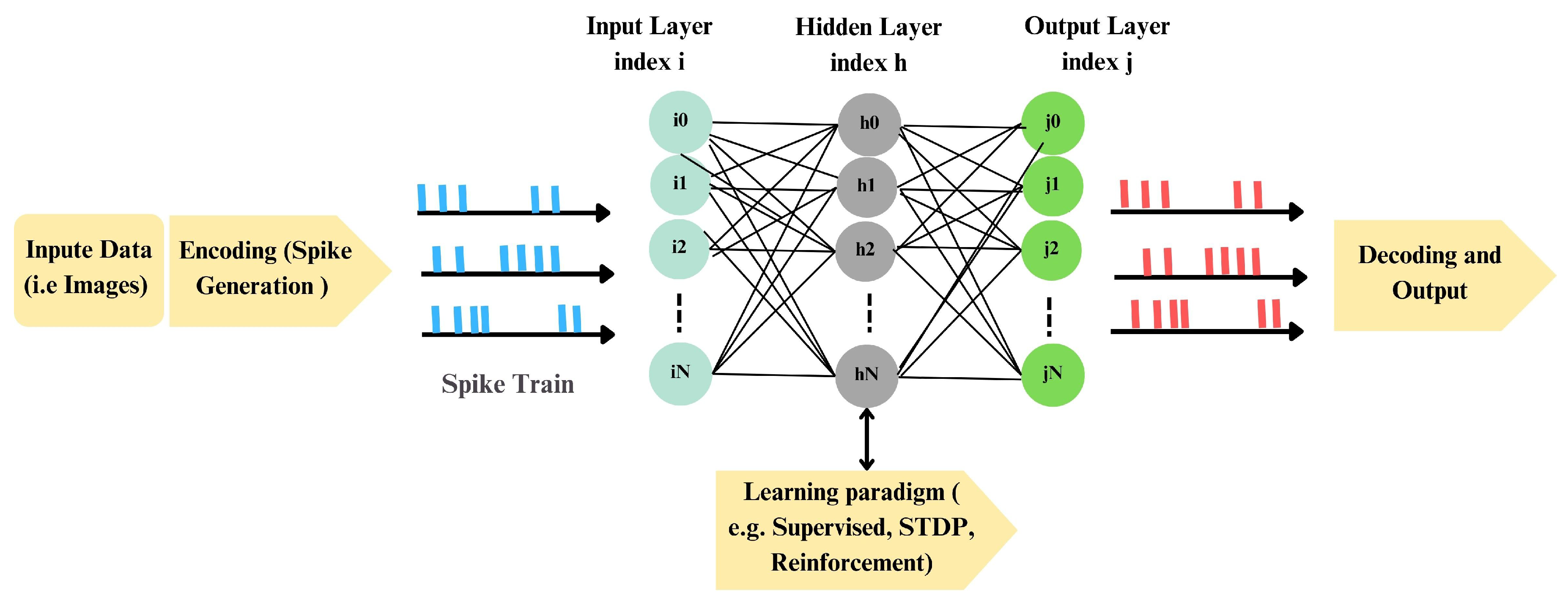
Figure 2.
Illustration of encoding using Rate, TTFS, and Burst coding. (1) Rate coding shows different firing rates for low, medium, and high stimulus intensities. (2) TTFS coding represents intensity by the latency to the first spike. (3) Burst coding shows variations in the number and duration of spikes.
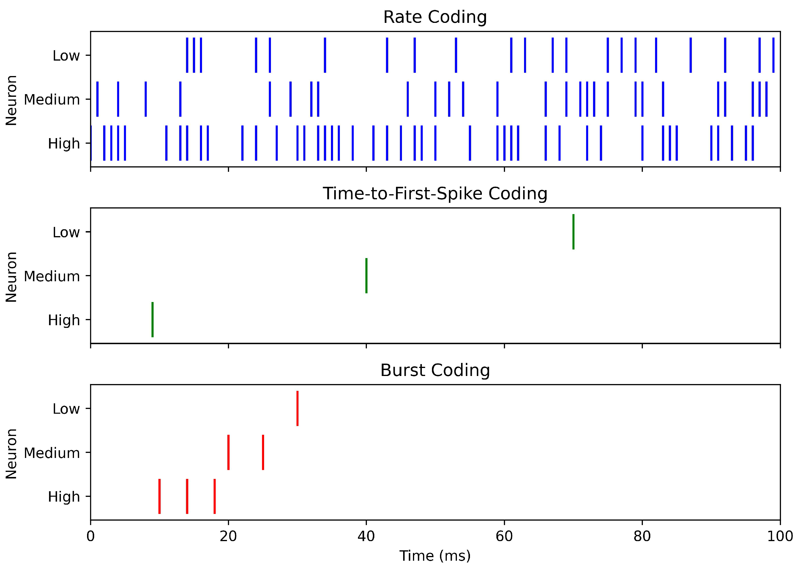
Figure 3.
Illustration of encoding using Inter-Spike Interval (ISI), N-of-M, Population, and PoFC coding. (1) ISI coding shows differences in inter-spike intervals across stimulus intensities. (2) N-of-M coding illustrates the number of spikes from a fixed set. (3) Population coding indicates the number of active neurons. (4) PoFC coding aligns spikes with specific phases of an oscillatory cycle.
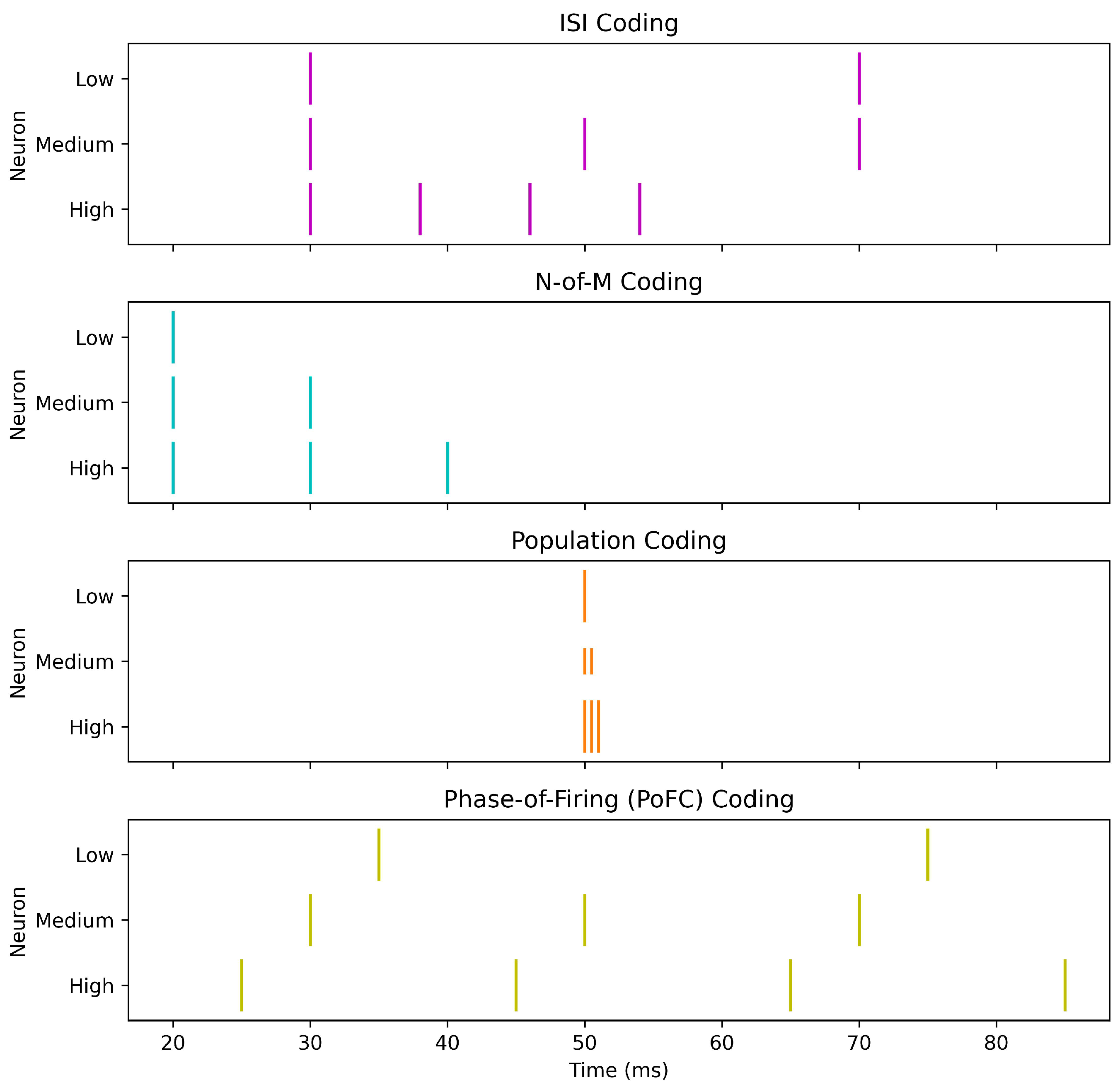
Figure 4.
encoding of a dynamic signal. The original noisy input and its reconstruction from spikes are shown; the delta stream highlights thresholded variations, illustrating high fidelity with reduced spikes.
Figure 4.
encoding of a dynamic signal. The original noisy input and its reconstruction from spikes are shown; the delta stream highlights thresholded variations, illustrating high fidelity with reduced spikes.
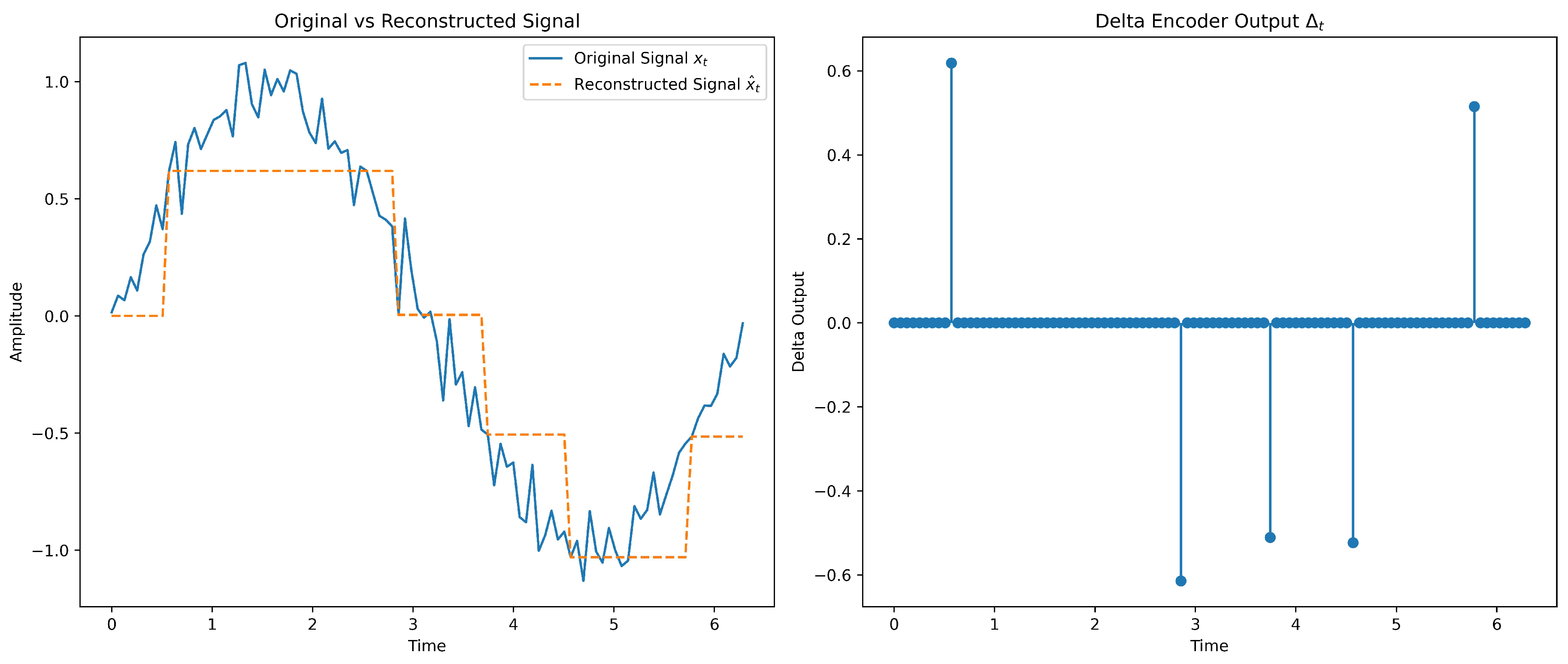
Figure 5.
Illustrative LIF trajectory: integrates synaptic input with passive leak toward , emits a spike at , and resets to .
Figure 5.
Illustrative LIF trajectory: integrates synaptic input with passive leak toward , emits a spike at , and resets to .
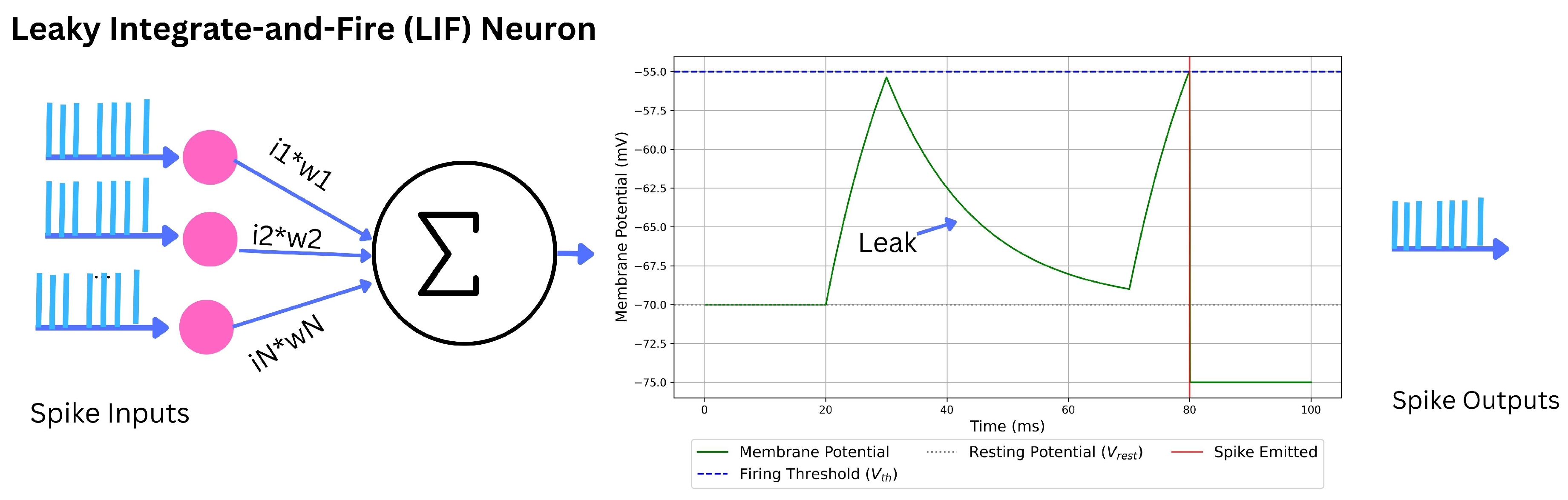
Figure 6.
Fully Connected Network (FCN) Architecture for the MNIST dataset.
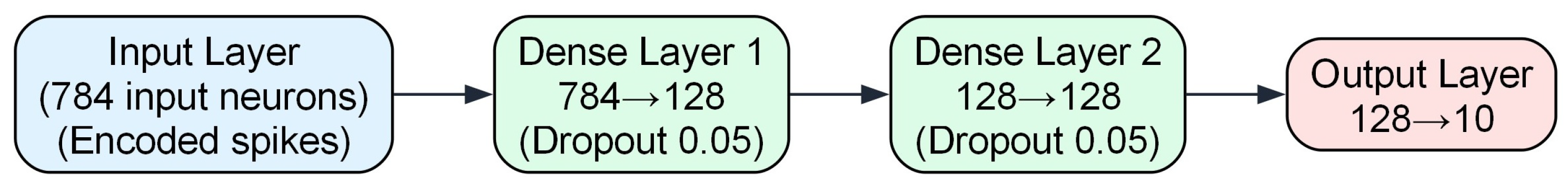
Figure 7.
VGG7 Network Architecture for the CIFAR-10 dataset. Abbreviations used: K for Kernel size, S for Stride, and P for Padding.
Figure 7.
VGG7 Network Architecture for the CIFAR-10 dataset. Abbreviations used: K for Kernel size, S for Stride, and P for Padding.
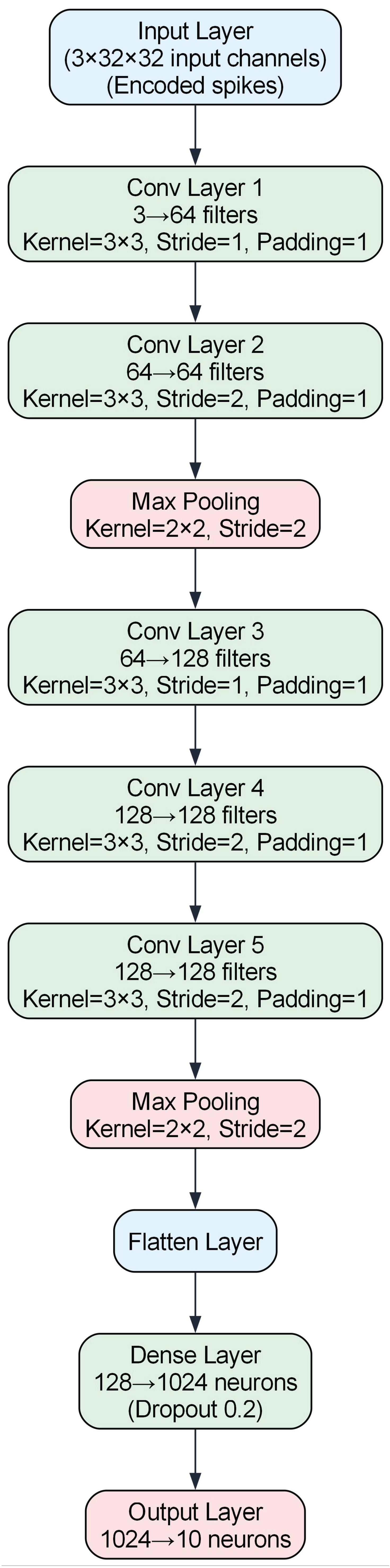

Table 1.
Summary of SNN encoding schemes reflecting the critical analysis in Section 2.1. Figure 2 and Figure 3 illustrate representative examples.
Table 1.
Summary of SNN encoding schemes reflecting the critical analysis in Section 2.1. Figure 2 and Figure 3 illustrate representative examples.
| Encoding Type | Main Applications | Complexity | Biological Plausibility | Advantages | Challenges |
|---|---|---|---|---|---|
| Rate Coding [38,75,78] | Image & signal processing; ANN-to-SNN conversion; resource-constrained inference | Low | High | Simple implementation; noise/adversarial robustness; hardware-friendly mapping from activations | Loses fine temporal structure; window-length/latency sensitivity; can require high spike counts that raise energy [80] |
| Direct Input Encoding [73,74,76,78,81] | Deep vision and real-time pipelines with large datasets; accuracy/latency–critical use | Moderate–High | Low | Fewer timesteps; preserves input fidelity; simplifies front end; fast inference | Not event driven; multi-bit input raises compute/energy; lower biological realism |
| Temporal Coding [14,24,38,76,82] | Rapid sensory processing; real-time decisions; fine temporal discrimination/patterns | High | High | High information per spike; low-latency responses; potentially energy efficient with sparse spiking | Sensitive to jitter/noise; complex decoding; training with precise timings is challenging |
| Population Coding [83,84] | Speech/audio; noisy environments; improving separability with simple classifiers | High | High | Noise robustness via redundancy; improved linear separability | More neurons increase energy; decoding large populations adds computational overhead |
| Encoding [74,78,85,86,87,88] | Dynamic signals (wearables, biomedical, streaming sensors); energy-aware neuromorphic platforms | Moderate–High | Moderate | Encodes changes (fewer spikes) with good fidelity; noise shaping; strong energy savings | Requires feedback-loop/circuit tuning; trade-offs among fidelity, latency, and energy |
| Burst Coding [13,75,89,90] | Biologically realistic simulations; temporally complex signals; long-activity tasks | Moderate–High | High | Rapid information transfer in spike packets; can be energy saving when bursts are well managed | Synchronizing bursts complicates decoding; scalability and parameter tuning on hardware |
| PoFC[87,91,92,93] | Spatial navigation/sensory processing with oscillations; high-fidelity temporal representation | High | High | Dense information per spike via phase; strong discriminability; potential spike-count/energy reduction | Requires precise global phase reference; sensitive to timing noise; complex decoding and STDP integration |
Table 2.
Summary of neuron models. Complexity and plausibility are qualitative: Very Low (V. Low), Low, Moderate (Mod.), Moderate–High (Mod.–High), High, Very High (V. High).
Table 2.
Summary of neuron models. Complexity and plausibility are qualitative: Very Low (V. Low), Low, Moderate (Mod.), Moderate–High (Mod.–High), High, Very High (V. High).
| Neuron Model | Main Applications | Complexity | Biological Plausibility | Advantages | Challenges |
|---|---|---|---|---|---|
| SRM [38,100] | STDP studies; analytical probes of SNNs; event-driven/hardware simulation | Low | Mod. | Kernel-based, tractable; separates synaptic and refractory effects; efficient | Limited subthreshold nonlinearities; requires kernel/threshold calibration |
| IF [101,104] | Baselines; large-scale SNNs; theoretical analysis | V. Low | Low | Extremely simple; fast; closed-form insights | Unrealistic integration (no leak); no adaptation/resonance |
| LIF [38,103] | Neuromorphic inference; brain–computer interfaces; large-scale simulations | Low | Mod. | Good accuracy–efficiency balance; event-driven; well-studied statistics | No intrinsic adaptation/bursting; linear subthreshold |
| ALIF [100,105] | Temporal/sequential tasks; speech-like streams; robotics control | Mod. | Mod. | Spike-frequency adaptation; better temporal credit assignment | Extra state and parameters; tuning sensitivity |
| EIF [104,106] | Fast fluctuating inputs; spike initiation studies; neuromorphic surrogates | Mod. | High | Sharp, smooth onset; improved gain/phase vs. LIF | Parameter calibration; stiffer near threshold |
| AdEx [107] | Cortical pattern repertoire; adapting/bursting cells; efficient yet rich neurons | Mod.–High | High | Diverse firing patterns with compact model; efficient integration | More parameters; careful numerical and hardware calibration |
| RF [111] | Resonance/phase codes; frequency-selective processing; edge sensing prototypes | Mod. | High | Captures subthreshold oscillations and resonance; phase selectivity | Phenomenological spike; added second-order state; parameter tuning |
| HH [97] | Biophysical mechanism studies; channelopathies; pharmacology; single-cell fidelity | V. High | V. High | Gold-standard fidelity; reproduces ionic mechanisms and refractoriness | Computationally expensive; stiff; many parameters |
| Izhikevich [39,89] | Large-scale networks with rich firing; cortical microcircuits; plasticity studies | Mod. | High | Wide repertoire at low cost; simple 2D form with reset | Lower biophysical interpretability; heuristic fitting |
| RF–Iz [111,116] | Phase-aware resonance with lightweight reset; recurrent SNNs; neuromorphic stacks | Mod. | High | Preserves phase; efficient event rules; toolchain support (Lava) | Phenomenological; calibration of ; still > IF/LIF cost |
| CUBA [98] | Large-scale SNNs; theory; fast prototyping; hardware with current-mode synapses | Low | Low | Very fast; analytically convenient; event-driven synapses independent of V | Ignores reversal/shunt; biases in high-conductance regimes vs. COBA |
| [88,116,117] | Energy-constrained streaming (audio/vision); edge sensing; –LIF layers | Mod. | Mod. | Sparse, error-driven spikes; low switching energy; good reconstruction | Feedback/threshold tuning; integration details for stability and latency |
Table 3.
Overview of learning algorithms in SNNs, summarizing their paradigms, typical applications, computational complexity, biological plausibility, key advantages, and main challenges.
Table 3.
Overview of learning algorithms in SNNs, summarizing their paradigms, typical applications, computational complexity, biological plausibility, key advantages, and main challenges.
| Algorithm Name | Learning Paradigm | Main Applications | Complexity | Biological Plausibility | Advantages | Challenges |
|---|---|---|---|---|---|---|
| SpikeProp [123] | Supervised | Temporal pattern recognition | Low | Low | Enables precise spike timing learning; first event-based backpropagation for SNNs | Limited to shallow networks; affected by spike non-differentiability |
| SuperSpike [124] | Supervised | Temporal pattern recognition; deep SNN training | Medium | Medium | Uses surrogate gradients; enables multilayer training | Requires careful surrogate design; added computational cost |
| SLAYER [120] | Supervised | Complex temporal data; sequence prediction | High | Medium | Addresses temporal credit assignment; handles sequences well | Computationally intensive; complex to implement |
| EventProp [125] | Supervised | Exact gradient computation; neuromorphic hardware | High | High | Computes exact gradients; efficient for event-driven processing | Complex discontinuity handling; implementation challenges |
| STDP [51,122] | Unsupervised | Pattern recognition; feature extraction | Low | High | Biologically plausible; local weight updates | Limited scalability; lower accuracy for large-scale tasks |
| aSTDP [126,127] | Unsupervised | Adaptive feature learning | Medium | High | Dynamically adapts learning parameters; robust | Parameter tuning complexity; additional computation |
| Multiplicative STDP [128] | Unsupervised | Weight updates scaled by current weight; prevents unbounded growth/decay | High | Medium | Improves biological plausibility; stabilizes learning | Requires careful parameter tuning |
| Triplet-STDP [129] | Unsupervised | Frequency-dependent learning | Medium | Medium | Captures multi-spike interactions; models frequency effects | Complex spike attribution; higher computation |
| R-STDP [52] | RL | Adaptive learning; decision making | Medium | High | Integrates reward signals; adaptive to reinforcement tasks | Requires carefully designed reward schemes |
| ReSuMe [142] | RL | Temporal precision learning | Medium | High | Combines supervised targets with reinforcement feedback | Dependent on reward design; non-gradient-based |
| e-prop [131] | RL | Temporal dependencies; complex dynamics | High | High | Tracks synaptic influence with eligibility traces | Computationally intensive; eligibility tracking complexity |
| SSTDP [132] | Hybrid | High temporal precision; visual recognition | Medium | High | Merges backpropagation and STDP; energy-efficient | Requires precise timing data; integration complexity |
| ANN-to-SNN Conversion [135,136] | Hybrid | Neuromorphic deployment | Medium | Low | Leverages pre-trained ANNs; fast deployment | Accuracy loss in conversion; parameter mapping issues |
Table 4.
ANN and SNN architectures for FCN and VGG7.
| Layer | FCN Architecture | VGG7 Architecture |
|---|---|---|
| Input Layer | 784 input neurons | 3 channels, pixels |
| Layer 1 | Dense, 128 neurons, | Conv, 64 filters, kernel, stride 1, padding 1 |
| Layer 2 | Dense, 128 neurons, | Conv, 64 filters, kernel, stride 2, padding 1 |
| – | Output, 10 neurons | Max Pooling, kernel, stride 2 |
| Layer 3 | — | Conv, 128 filters, kernel, stride 1, padding 1 |
| Layer 4 | — | Conv, 128 filters, kernel, stride 2, padding 1 |
| Layer 5 | — | Conv, 128 filters, kernel, stride 2, padding 1 |
| – | — | Max Pooling, kernel, stride 2 |
| Flatten Layer | — | Flatten feature maps |
| Layer 6 | — | Dense, 1024 neurons, |
| Layer 7 | Output, 10 neurons | Output, 10 neurons |
| Special Components | Weight Normalization, Weight Scaling | Weight Normalization, Weight Scaling |
| Total Parameters | ∼118,016 | ∼548,554 |
| Frameworks Used | PyTorch for ANNs; Lava, Norse, SpikingJelly for SNNs | PyTorch for ANNs; Lava, Norse, SpikingJelly for SNNs |
Table 5.
hyperparameters for ANN and SNN models on FCN and VGG7 architectures.
| Parameter | ANN (FCN/VGG7) | SNN (FCN) | SNN (VGG7) |
|---|---|---|---|
| Optimizer | Adam | Adam | Adam |
| Learning rate | 0.001 | 0.001 | 0.001 |
| Weight decay | |||
| Loss function | Cross-Entropy | CrossEntropyLoss | CrossEntropyLoss |
| Number of epochs | FCN: 100; VGG7: 150 | 100 | 150 |
| Batch size | 64 | 64 | 64 |
| Dropout rate | FCN: 5%; VGG7: 20% | 5% | 20% |
| Activation function | ReLU | — | — |
| Weight initialization | PyTorch defaults | — | — |
| Neuron parameters | — | Threshold (): 1.25 Current decay: 0.25 Voltage decay: 0.03 Tau gradient: 0.03 Scale gradient: 3 Refractory decay: 1 |
Threshold (): 0.5 Current decay: 0.25 Voltage decay: 0.03 Tau gradient: 0.03 Scale gradient: 3 Refractory decay: 1 |
Table 6.
Maximum classification accuracies (%) on FCN with MNIST dataset.
| Neuron type | Time steps | Rate encoding | TTFS | Direct coding | Burst coding | PoFC | R-NoM | |
|---|---|---|---|---|---|---|---|---|
| ANN (baseline) | – | 98.23% | ||||||
| IF | 8 | 97.20 | 86.60 | 97.70 | 78.90 | 80.00 | 71.20 | 72.20 |
| 6 | 97.10 | 90.00 | 97.60 | 88.10 | 91.00 | 78.50 | 74.00 | |
| 4 | 96.90 | 92.00 | 97.40 | 86.80 | 88.40 | 79.80 | 76.80 | |
| LIF | 8 | 97.00 | 86.50 | 97.40 | 81.90 | 80.06 | 72.10 | 71.00 |
| 6 | 96.90 | 90.00 | 97.50 | 90.00 | 91.10 | 77.70 | 73.00 | |
| 4 | 96.90 | 92.00 | 97.20 | 88.60 | 83.30 | 82.30 | 75.50 | |
| ALIF | 8 | 97.30 | 96.40 | 96.50 | 97.10 | 97.14 | 92.70 | 58.00 |
| 6 | 96.60 | 96.10 | 96.30 | 97.00 | 97.00 | 92.90 | 57.00 | |
| 4 | 96.40 | 96.70 | 96.30 | 97.00 | 96.90 | 93.00 | 46.00 | |
| CUBA | 8 | 97.66 | 97.10 | 97.40 | 97.60 | 79.50 | 94.10 | 68.00 |
| 6 | 97.56 | 97.00 | 97.18 | 97.50 | 79.30 | 94.10 | 66.50 | |
| 4 | 97.20 | 96.30 | 96.40 | 97.30 | 96.80 | 93.40 | 56.00 | |
| 8 | 98.10 | 97.90 | 98.00 | 88.00 | 88.30 | 95.00 | 86.70 | |
| 6 | 97.80 | 97.50 | 98.00 | 88.50 | 97.90 | 87.40 | 86.00 | |
| 4 | 97.90 | 97.50 | 97.70 | 98.00 | 97.90 | 87.80 | 64.00 | |
| RF | 8 | 93.00 | 86.80 | 90.05 | 97.20 | 92.20 | 85.80 | 52.00 |
| 6 | 92.60 | 88.70 | 92.00 | 79.00 | 92.00 | 84.90 | 50.00 | |
| 4 | 93.00 | 88.00 | 91.60 | 53.00 | 91.70 | 83.90 | 47.70 | |
| RF-Iz | 8 | 97.70 | 47.00 | 79.60 | 97.70 | 50.00 | 94.90 | 48.00 |
| 6 | 97.55 | 87.70 | 97.40 | 97.70 | 97.40 | 94.80 | 69.70 | |
| 4 | 97.00 | 96.40 | 96.00 | 97.20 | 96.80 | 93.00 | 74.00 | |
| EIF | 8 | 96.70 | 94.60 | 96.50 | 97.50 | 96.30 | 95.20 | 88.10 |
| 6 | 96.20 | 94.90 | 96.20 | 97.60 | 96.00 | 94.50 | 86.70 | |
| 4 | 96.55 | 95.80 | 96.60 | 97.50 | 96.40 | 95.10 | 87.70 | |
| AdEx | 8 | 96.50 | 94.70 | 96.50 | 97.40 | 96.70 | 95.40 | 89.50 |
| 6 | 96.40 | 95.00 | 96.40 | 97.50 | 96.80 | 95.30 | 89.20 | |
| 4 | 96.00 | 95.90 | 96.44 | 97.39 | 96.80 | 95.20 | 88.50 | |
Table 7.
Total energy consumption during inference on MNIST dataset (joules per sample).
| Neuron type | Time steps | Rate encoding | TTFS | Direct coding | Burst coding | PoFC | R-NoM | |
|---|---|---|---|---|---|---|---|---|
| IF | 8 | |||||||
| 6 | ||||||||
| 4 | ||||||||
| LIF | 8 | |||||||
| 6 | ||||||||
| 4 | ||||||||
| ALIF | 8 | |||||||
| 6 | ||||||||
| 4 | ||||||||
| CUBA | 8 | |||||||
| 6 | ||||||||
| 4 | ||||||||
| 8 | ||||||||
| 6 | ||||||||
| 4 | ||||||||
| RF | 8 | |||||||
| 6 | ||||||||
| 4 | ||||||||
| RF-Iz | 8 | |||||||
| 6 | ||||||||
| 4 | ||||||||
| EIF | 8 | |||||||
| 6 | ||||||||
| 4 | ||||||||
| AdEx | 8 | |||||||
| 6 | ||||||||
| 4 |
Table 8.
Maximum classification accuracies (%) on VGG7 with CIFAR-10 dataset.
| Neuron Type | Time Steps | Rate Encoding | TTFS | Direct Coding | Burst Coding | PoFc | R-NoM | |
|---|---|---|---|---|---|---|---|---|
| ANN (Baseline) | – | 83.60% | ||||||
| IF | 2 | 57.00 | 60.00 | 62.00 | 74.00 | 60.00 | 57.00 | 29.00 |
| 4 | 56.50 | 62.00 | 65.00 | 74.50 | 64.00 | 65.00 | 27.00 | |
| 6 | 57.00 | 62.50 | 65.00 | 74.50 | 64.50 | 68.00 | 30.00 | |
| LIF | 2 | 50.00 | 61.50 | 62.50 | 74.30 | 57.60 | 59.00 | 28.00 |
| 4 | 51.00 | 62.00 | 64.50 | 74.50 | 61.00 | 63.00 | 23.00 | |
| 6 | 50.00 | 59.50 | 65.00 | 74.00 | 61.50 | 67.00 | 21.00 | |
| ALIF | 2 | 10.00 | 10.00 | 10.00 | 10.00 | 10.00 | 10.00 | 10.00 |
| 4 | 39.00 | 34.00 | 20.00 | 46.00 | 20.00 | 27.00 | 14.00 | |
| 6 | 51.00 | 38.00 | 28.00 | 49.00 | 27.00 | 29.00 | 24.00 | |
| CUBA | 2 | 10.00 | 10.00 | 10.00 | 10.00 | 10.00 | 10.00 | 10.00 |
| 4 | 34.00 | 50.00 | 33.50 | 40.00 | 30.00 | 24.00 | 25.00 | |
| 6 | 45.00 | 43.00 | 40.00 | 50.00 | 30.00 | 31.00 | 27.00 | |
| 2 | 57.00 | 72.00 | 56.00 | 83.00 | 57.00 | 57.00 | 30.00 | |
| 4 | 61.00 | 72.00 | 66.00 | 78.00 | 66.00 | 62.00 | 27.00 | |
| 6 | 60.00 | 72.50 | 68.00 | 79.00 | 66.00 | 67.00 | 24.00 | |
| RF | 2 | 10.00 | 10.00 | 10.00 | 10.00 | 10.00 | 10.00 | 10.00 |
| 4 | 22.00 | 10.00 | 10.00 | 42.00 | 10.00 | 10.00 | 10.00 | |
| 6 | 37.00 | 36.00 | 32.00 | 47.00 | 39.00 | 37.00 | 31.00 | |
| R&F Iz | 2 | 10.00 | 10.00 | 10.00 | 10.00 | 10.00 | 10.00 | 10.00 |
| 4 | 10.00 | 10.00 | 10.00 | 33.00 | 10.00 | 10.00 | 10.00 | |
| 6 | 45.00 | 37.00 | 30.00 | 39.00 | 32.00 | 32.00 | 27.00 | |
| EIF | 2 | 58.50 | 56.00 | 53.50 | 70.00 | 58.50 | 54.00 | 25.00 |
| 4 | 59.50 | 64.00 | 60.00 | 69.00 | 57.00 | 57.00 | 22.50 | |
| 6 | 60.00 | 65.00 | 61.00 | 68.50 | 53.50 | 60.00 | 24.00 | |
| AdEx | 2 | 59.00 | 55.50 | 60.00 | 69.50 | 58.50 | 54.00 | 27.00 |
| 4 | 60.00 | 62.00 | 61.50 | 70.00 | 56.50 | 59.00 | 29.00 | |
| 6 | 60.50 | 63.00 | 60.50 | 70.10 | 52.00 | 61.00 | 25.50 | |
Table 9.
Total Energy Consumption during Inference on CIFAR-10 Dataset (joules per sample).
| Neuron type | Time steps | Rate encoding | TTFS | Direct coding | Burst coding | PoFC | R-NoM | |
|---|---|---|---|---|---|---|---|---|
| IF | 2 | |||||||
| 4 | ||||||||
| 6 | ||||||||
| LIF | 2 | |||||||
| 4 | ||||||||
| 6 | ||||||||
| ALIF | 2 | 0 | 0 | 0 | 0 | 0 | 0 | 0 |
| 4 | ||||||||
| 6 | ||||||||
| CUBA | 2 | 0 | 0 | 0 | 0 | 0 | 0 | 0 |
| 4 | ||||||||
| 6 | ||||||||
| 2 | ||||||||
| 4 | ||||||||
| 6 | ||||||||
| RF | 2 | 0 | 0 | 0 | 0 | 0 | 0 | 0 |
| 4 | 0 | 0 | 0 | 0 | ||||
| 6 | ||||||||
| RF-Iz | 2 | 0 | 0 | 0 | 0 | 0 | 0 | 0 |
| 4 | 0 | 0 | 0 | 0 | 0 | 0 | ||
| 6 | ||||||||
| EIF | 2 | |||||||
| 4 | ||||||||
| 6 | ||||||||
| AdEx | 2 | |||||||
| 4 | ||||||||
| 6 |
Table 10.
Maximum classification accuracies (%) on CIFAR-10 dataset with varying thresholds. The highest accuracy for each encoding scheme is highlighted in bold.
Table 10.
Maximum classification accuracies (%) on CIFAR-10 dataset with varying thresholds. The highest accuracy for each encoding scheme is highlighted in bold.
| Encoding scheme | Threshold | 2 steps | 4 steps | 6 steps |
|---|---|---|---|---|
| Rate encoding | 0.1 | 58.50 | 59.50 | 60.00 |
| 0.5 | 47.00 | 53.00 | 47.50 | |
| 0.75 | 40.00 | 41.00 | 27.00 | |
| TTFS encoding | 0.1 | 56.00 | 64.00 | 65.00 |
| 0.5 | 57.00 | 65.50 | 67.50 | |
| 0.75 | 54.00 | 65.00 | 55.00 | |
| encoding | 0.1 | 53.50 | 60.00 | 61.00 |
| 0.5 | 39.00 | 38.50 | 54.00 | |
| 0.75 | 51.50 | 30.00 | 51.00 | |
| Direct coding | 0.1 | 70.00 | 69.00 | 68.50 |
| 0.5 | 68.00 | 67.50 | 66.00 | |
| 0.75 | 16.00 | 17.00 | 15.00 | |
| Burst coding | 0.1 | 58.50 | 57.00 | 53.50 |
| 0.5 | 32.00 | 56.00 | 60.00 | |
| 0.75 | 51.00 | 57.00 | 55.00 | |
| PoFC | 0.1 | 54.00 | 57.00 | 60.00 |
| 0.5 | 42.50 | 53.50 | 56.00 | |
| 0.75 | 17.00 | 39.50 | 20.00 | |
| R-NoM | 0.1 | 25.00 | 22.50 | 24.00 |
| 0.5 | 28.00 | 28.00 | 29.50 | |
| 0.75 | 29.00 | 28.50 | 28.00 |
Table 11.
Energy consumption (joules) on CIFAR-10 dataset with varying thresholds. The lowest energy consumption for each encoding scheme is highlighted in bold.
Table 11.
Energy consumption (joules) on CIFAR-10 dataset with varying thresholds. The lowest energy consumption for each encoding scheme is highlighted in bold.
| Encoding scheme | Threshold | 2 steps | 4 steps | 6 steps |
|---|---|---|---|---|
| Rate encoding | 0.1 | |||
| 0.5 | ||||
| 0.75 | ||||
| TTFS encoding | 0.1 | |||
| 0.5 | ||||
| 0.75 | ||||
| encoding | 0.1 | |||
| 0.5 | ||||
| 0.75 | ||||
| Direct coding | 0.1 | |||
| 0.5 | ||||
| 0.75 | ||||
| Burst coding | 0.1 | |||
| 0.5 | ||||
| 0.75 | ||||
| PoFC | 0.1 | |||
| 0.5 | ||||
| 0.75 | ||||
| R-NoM | 0.1 | |||
| 0.5 | ||||
| 0.75 |
Disclaimer/Publisher’s Note: The statements, opinions and data contained in all publications are solely those of the individual author(s) and contributor(s) and not of MDPI and/or the editor(s). MDPI and/or the editor(s) disclaim responsibility for any injury to people or property resulting from any ideas, methods, instructions or products referred to in the content. |
© 1996 by the authors. Licensee MDPI, Basel, Switzerland. This article is an open access article distributed under the terms and conditions of the Creative Commons Attribution (CC BY) license (https://creativecommons.org/licenses/by/4.0/).
Copyright: This open access article is published under a Creative Commons CC BY 4.0 license, which permit the free download, distribution, and reuse, provided that the author and preprint are cited in any reuse.


