Submitted:
23 September 2025
Posted:
24 September 2025
You are already at the latest version
Abstract
In recent decades, the data collection technologies have evolved to facilitate the monitoring and improvement of numerous activities and processes in everyday human life. The evolution is propelled by the advancement of artificial intelligence (AI), which aims to emulate human intelligence in the execution of related tasks. The remarkable success of deep learning (DL) and computer vision (CV) on image data prompted researchers to consider its application to time series and multivariate data. In this context, time-series imaging has been identified as the research field for the transformation of time-series data (one-dimensional data format) into images (two-dimensional data format). State-of-art techniques of time-series imaging are Recurrence Plot (RP), Gramian Angular Field (GAF), and Markov Transition Field (MTF). This paper proposes a novel, robust and simple technique of time-series imaging using Grayscale Fingerprint Features Field Imaging (G3FI). The novel technique is distinguished by its low resolution of the resulting image and the simplicity of the transformation procedure. The efficacy of the novel and state-of-the-art techniques for enhancing the performance of CNN-based classification models on time-series datasets is thoroughly examined and compared.
Keywords:
deep learning
; convolutional neural networks
; computer vision
; image classification
; imaging time series
; grayscale fingerprint features field imaging
1. Introduction
With enormous and unprecedented advances in smart data and information collection technologies, such as Internet of Things (IoT), cell phones, GPS, Bluetooth, and smart cards, especially in hard-to-reach areas, and their processing techniques, the integration of these technologies is becoming easier and more popular in human daily life and related activities, such as industry, healthcare, finance, and other fields [1,2,3]. The intelligent collection of these data is typically executed over specific, time-ordered intervals. For this reason, these data are generally referred to as time-series data [4]. This enormous growth is usually accompanied by the increasing availability of data. Some of the collected, created or generated data are strongly related to the specific task space, namely informative, while other data could be redundant, namely non-informative, in terms of the desired task performance. Consequently, this phenomenon results in a diminution of storage capacity and an escalation in the computing time of the corresponding processing operations due to non-informative data. Therefore, it is necessary to define the valuable and informative data among the collected raw data in order to reduce associated high-cost storage and computing time of the operations [1,2,4]. Extracting actionable information from the raw data collected and processing and analyzing it leads to a wide range of tasks such as current state representation, future state prediction, automation opportunity detection, anomaly detection, predictive and predictive maintenance, condition monitoring, cybersecurity, and human activity recognition [2,3].
The analysis of time-series data for the purpose of obtaining this useful information can be categorized as either conventional or data-driven [1,2]. Statistical models such as exponential smoothing and ARIMA as examples of conventional models can be modified by "non-data hungry" and computationally cheap approaches. However, they 1) have low generalization ability to prescribe the data generation process of the series, 2) show limited learning ability, and 3) are usually unable to extract the valuable information hidden in the large data sets. Addressing the tasks associated with analyzing time-series data as data grow requires the application of scalable, robust, and efficient processing and analysis tools. These requirements cannot be met by conventional methods. Therefore, AI-based models are strongly recommended for these purposes. Due to the specifications (e.g., modeling of nonlinear relationships, automatic pattern recognition, scalability) of AI-based models, these models are better suited and more efficient than conventional models (statistical, signal processing, etc.) to perform the tasks related to the large data amounts [1,2,4,5,6]. AI-based models are Machine Learning (ML) and Deep Learning (DL) as illustrated in Figure 1, which shows also the parental relation among them [7].
- They require manual feature engineering.
- They are highly subjective.
- They do not generalize well in other scenarios.
- They require a high level of expertise.
- They are time-consuming during the data preprocessing with more than 50% of the whole data processing process.
- They are influenced by human factors.
To address these issues relating ML models, DL models have been introduced as a powerful framework with high properties for generalizability, objectivity, performance, and integration of automated feature extraction and final classification processes in a single shot [15,16]. For example, recurrent neural networks (RNNs), which are one of the many different DL structures, have been shown to be powerful in modeling time-series data [16,17]. Specifically, the long short-term memory (LSTM) structure has been shown to possess a high learning capability from information within the time sequence that is distant in the past [18].
Due to the increasing availability and complexity of time-series sequences, RNN/LSTM models cannot learn from the far back information of these long sequences to achieve the most accurate modeling without loss of information. To solve this problem, the technique of "Imaging/Image-Encoded Time Series" is introduced to preserve all the information even in long sequences. With this novel technique, the remarkable performances of convolutional neural networks (CNN) in computer vision (CV) can be used to accomplish the tasks related to time-series prediction and classification [19,20,21,22,23].
2. Review of Related Work and Basic Methods
2.1. Definitions
The types of time series can be basically classified according to the number of descriptive variables/features measured/observed during the sampling period [24]:
- Univariate time series: only one descriptive variable/feature has been measured and observed over time.
- Multivariate time series: several descriptive variables/features have been measured and observed over time.
During the sampling time of the different descriptive characteristics of the considered process or phenomenon, the related multivariate time-series dataset consists of the many samples stored in the row, which represents the considered observation/measurement time, and the different descriptive features stored in the columns for each sample. Therefore, the imaging time series can be defined as the mathematical process that transfers each sample of a multivariate time series, considered as a vector of descriptive features, into a matrix format that can be considered as a 2D image in the context of DL and CV systems [20,25].
2.2. Imaging Time-Series Techniques
In this section, an exposition of state-of-the-art transformation techniques is provided. These techniques include recurrence plot, Gramian angular summation/difference fields, and Markov transition field.
2.2.1. Recurrence Plot (RP)
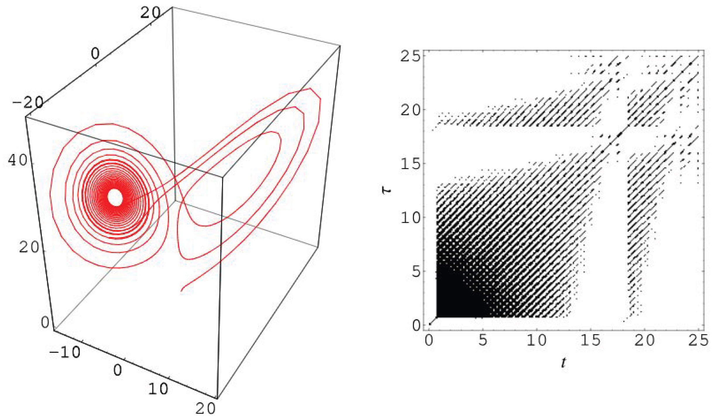
The RP has been developed by Eckmann et al. [26] to visualize the recurrence of state () in a 2D or 3D phase/state space. For the higher than 3D phase/state space, it can only be visualized by projecting into the two- or three-dimensional subspaces.
Ramirez-Amaro et al. [27] stated: „The recurrence plot analysis provides us a way to visualize and quantify the dynamical systems behavior over the time. The construction of a recurrence plot (RP) from a time series begins with the determination of the trajectory of the system through phase-space. Seven different measures are extracted from the RP. These measures are obtained from diagonal and vertical structures of the RP.”
The RP allows us to trace and study the trajectory of the m-dimensional phase space through a two-dimensional representation of its repetitions, where the trajectory of the repetition of a state () over time between the initial time (i) and the considered time (j) through the original m-dimensional phase space is mathematically projected into a two-dimensional square matrix whose elements are:
- Ones (recurrent state: and
- Zeros (transient state: .
This matrix is represented graphically by black (recurrent state) and white (transient state) points, in the 2D time axis-based plot as illustrated in Figure 2. Consquently, the goal of RP is to graphically display non-stationarity (changing of the related statistical properties over time) in time series.
In dynamical systems, a trajectory is defined as the set of points representing the future states resulting from a given initial state in the phase or state space [24,28]:
where
- m is the dimensions of the considered phase space.
- n is the length of the trajectory through the phase space/number of the future states resulting from a given initial state in phase space.
- : Considered time delay.
Figure 2.
Visualization of the recurrence of state () in a 2D or 3D Phase/State space [29].
Figure 2.
Visualization of the recurrence of state () in a 2D or 3D Phase/State space [29].
Therefore, the application of RP analysis as an imaging time series technique aims to extract the trajectories of the time series and then calculate the binarized pairwise distance matrix between them as a recurrence representation in the phase/state space. This matrix is denoted as R to build the recurrence diagram for RP as follows [24,28]:
where
- is the binarized pairwise distance matrix of the trajectory of the recurrence of a state () between the initial time point i and the time point j over time in the m-dimensional phase space.
- is the Heaviside function.
- is the recurrence threshold.
- is the norm operator (normally the Euclidean norm is used).
2.2.2. Gramian Angular Field (GAF)
The GAF represents the temporal correlation between each pair of time series values to produce a meaningful image. The core of GAF is a Gramian matrix, denoted by G, which is a useful tool in linear algebra and geometry to calculate the linear dependence of a set of the vectors. The Gramian matrix of a vectors set is a matrix defined by the dot product, also known as the inner product, of each pair of vectors to measure the degree of similarity between them. The dot/inner product between two vectors u and v is defined as:
If u and v vectors are unit vectors, whose norm is 1, then the related inner product is characterized exclusively by the angle () (expressed in radians) between two vectors as follows. The Gramian matrix of (n) unit vectors is defined as:
The closer the () angle between the two considered vectors is to:
- , these two vectors are similar.
- , these two vectors are orthogonal.
- , these two vectors are opposite.
The Procedure of the GAF technique of the time series, whose length is l samples, consists of the following steps as shown in Figure 5 [19]:
- A Min-Max Scaling process is applied to transfer the time series onto the range;
- A Polar Encoding of each sample () within the scaled time series is calculated by:whre is the time stamp.
-
The Gramian matrix can be defined by two types of fields that encode the time series signals into images:
- Gramian Angular Summation Field (GASF) matrix:
- Gramian Angular Difference Field (GADF) matrix:
- Generation of the related GAF Image.
Figure 6 shows an example of the GASF and GADF images of the time series.
2.2.3. Markov Transition Field (MTF)
The MTF represents the transition probabilities between each pair of values in the discretized time series to obtain a relevant image. The Markov Transition Matrix, also known as stochastic or probability matrix and denoted by P, is the core of the MTF. This matrix is a square matrix representing the transition probabilities of the state to another during one time step/unit of motion in the phase/state space of the dynamical system as [30]:
where
- is the probability of the transition of the () form (i) state to (j) state during one time step/unit of motion in the state space.
- Q is the number of states in/size of the state space of the considered dynamical system.
The MTF method as the imaging time-series technique consists of the following steps as shown in Figure 7 [19,30]:
- Discretize the time series to Q quantile bins (e.g., A, B, C and D as in Figure 7).
- Build the Markov transition matrix.
- Compute transition probabilities.
- Compute the Markov transition field.
- Compute an aggregated MTF.
2.3. Convolutional Neural Networks as Deep Learning Systems Applied to Imaging Time-Series Datasets
2.3.1. Convolutional Neural Networks (CNN)
The visual cortex-based neocognitron network, proposed by Fukushima in 1980 [31], was further developed into CNN by LeCun et al. [32] with the famous LeNet-5 architecture to recognize the handwritten digits as illustrated in Figure 8. The general structure of CNN consists of the following blocks as illustrated in Figure 9 [33,34].
-
Feature Extraction:
- Convolution Layer: Basically, a convolution is defined as a mathematical operation in which two sets of information are merged to create a new set that contains more informative information about the task at hand. In this sense, the first information set is considered as an image represented by a 2D matrix with one or three channels. The second information set is a convolution filter, usually a square matrix with dimensions of 2, 3, etc., that extracts specific features. These features can be low-level (such as contours, edges, angles, and colors) or high-level (such as shapes and objects). The extracted features are collected together to create a 2D "feature map." The convolution process can also be applied to the feature map generated from the previous layer to create a new feature map with more complex and intricate features than the original.
- Nonlinear Activation Layer: It consists of nonlinear functions, such as the rectified linear unit (ReLU) and sigmoid functions. The correlation between the convolution process and the nonlinearity process can perform the following tasks: 1) enable the network/model to learn/build complex representations and relationships with a "nonlinearity property" of the input/output data/information and 2) prevent the exponential growth of the computations required to run the neural network.
- Pooling Layer: In this step, the size of the feature map generated by the (Convolution + ReLU) layer is subsampled by aggregating features from local regions to learn invariant features and reduce computational complexity. In this process, the m-square matrix (usually or ) is shifted over the processed feature map using a predefined step called stride. For each shift, a value (e.g., average, maximum, or minimum) is computed and substituted in place of the originally processed values in the new feature map.
The sequence of layers (convolutional layer, nonlinear activation function, and pooling), called hidden layers, can be stacked several times, and their final output yields the feature map. The deeper the feature extraction block of the CNN, the more complex the feature map, i.e., the feature map starts with low-level features and then becomes more complex as it passes through each hidden layer until it reaches high-level features at the end of the feature extraction block. - Flattening Layer: Since the final output of the last (Convolution + ReLU + Pooling) sequence as the last layer in the feature extraction stage has the format of a 2D matrix and also the input of the classification stage in the CNN model has the format of a 1D matrix, the process "Flatten" should be applied.
- Classification: The extracted and flattened features maps of the considered states will be processed by the Fully Connected (FC) network, which consists of the several feedforward layers
- Probabilistic Distribution: To bring probabilistic distribution of the considered classes, a SoftMax Activation function is usually applied.
The CNN structure can also include other types of layers, such as dropout and/or Batch Normalization, to solve the problems such as overfitting. The popular state-of-the-art CNN architectures are: 1) LeNet-5 (1998), 2) AlexNet (2012), 3) ZFNet (2013), 4) GoogLeNet/Inception (2014), 5) VGGNet (2014), and 6) ResNet (2015) [34].
2.3.2. CNN Classification Systems Based on Time Series-to-Image Encoding
A brief review of some CNN classification systems based on time series-to-image encoding, as proposed in [1,21], is provided below:
-
Gross et al. [1] suggested the following concepts for building the classification system of the time series as illustrated in Figure 10 [1]:
- GAF, GASF, and GADF as time-series imaging techniques, which will be separately used to image the considered time-series dataset and
- Benchmarking transfer learning strategies, which aims to improve the learning of new task through the transfer of knowledge from a related task that has already been learned (such as VGG16, VGG19, ResNet50V2 and Xception).
To evaluate the transfer learning strategies for benchmarking time-series imaging, the following datasets were used, whose numerical specifications are listed in Table 1 [35]:- (a)
- Computers: These problems were taken from data recorded as part of government sponsored study called Powering the Nation. The intention was to collect behavioral data about how consumers use electricity within the home to help reduce the UK’s carbon footprint. The data contains readings from 251 households, sampled in two-minute intervals over a month. Each series is length 720 (24 hours of readings taken every 2 minutes). Classes are Desktop and Laptop.
- (b)
- DodgerLoopGame: The traffic data are collected with the loop sensor installed on ramp for the 101 North freeways in Los Angeles. This location is close to Dodgers Stadium; therefore the traffic is affected by volume of visitors to the stadium.- Class 1: Normal Day - Class 2: Game Day.
- (c)
- ECG200: Each series traces the electrical activity recorded during one heartbeat. The two classes are a normal heartbeat and a Myocardial Infarction.
- (d)
- AbnormalHeartbeat: Heartbeat recordings were gathered from both the iStethoscope Pro iPhone app and from clinical trials using digital stethoscope DigiScope. The time series represent the change in amplitude over time during an examination of patients suffering from any four common arrhythmias.
-
Buz et al. [21] developed another approach and application of time series-to-image transformation methods for classifying underwater objects (sonar signals), as shown in Figure 11. The sonar dataset developed by Gorman et al. [36] was used to evaluate the Buz et al.’s method. This dataset contains the signals reflected from cylindrical mines and cylindrical rocks resembling these mines from different angles. The size of the dataset is 208 samples in the format of the time series, where 111 samples belong to cylindrical mines and 97 samples to cylindrical rocks. The length of each time series is 60 numbers, ranging from 0.0 to 1.0. Each number represents the energy collected over a fixed period in a given frequency band [36].The core of the comparative analysis is the conversion of the sonar time-series dataset into the related and individual 2D image dataset by means of the separate application of the GASF, MTF, and RP techniques. Then, the three related 2D image datasets are merged to generate the 3D image for each sample in the sonar dataset, as shown in Figure 14. The resulting 3D image dataset is used to train and evaluate the CNN architecture shown in Figure 12.
3. Novel Approach of Time Series-to-Image Encoding for Convolutional Neural Networks-based Classification
3.1. Grayscale Fingerprint Features Field Imaging Techniques
3.1.1. Motivation
Based on the mathematical background and the transformation processes used in the state of the art of imaging time-series techniques, we found that:
- The transformation processes are characterized by a high degree of complexity.
- The resulting image structure exhibits diagonal symmetry, resulting in the presence of redundant and duplicated information.
- The resolution of the image is directly proportional to the square of the number of descriptive features of the time-series data under consideration. Consequently, as the number of features increases, the image resolution improves. However, this enhancement in resolution necessitates a proportional increase in the time required to process the image, thereby achieving the desired objectives, such as classification.
To avoid the complexity and high computation time associated with the state-of-art techniques of time-series imaging, the following solutions are proposed:
- Only two simple steps-based transformation process is applied to transfer the descriptive features/variables of each sample of the time series into the 2D image.
- The resulting image has a non-symmetric property and its resolution is equal to the number of descriptive features/variables of the transformed sample.
These solutions can be realized by a Grayscale Fingerprint Features Field Imaging (G3FI) as a novel imaging time-series technique.
3.1.2. Methodology
The vector of the l descriptive features of each considered sample can be defined as:
where
- is the descriptive feature.
- l is the number of the used descriptive features/number of the columns of the multivariate time-series dataset.
The proposed process of generation the corresponding grayscale fingerprint is as follows:
-
Grayscale-based normalizing process of descriptive features of each considered sample by:leading to new feature values between zero (black) and 255 (white), with:
- is the normalized/scaled vector of the descriptive features of each considered sample.
- is the minimum value of the descriptive features of each considered sample.
- is the maximum value of the descriptive features of each considered sample.
- 255 is the scalar of grayscale processing.
-
Generation process of G3FI image () by reshaping (Reshape) the grayscale normalized vector of each considered sample into the () matrix as follows:where
- is the reshaping process of the grayscale normalized/scaled vector into () matrix to generate G3FI Image.
- K is the number of rows in the G3FI image matrix().
- L is the number of columns in the G3FI image matrix ().
The term "fingerprint" is used in the context of this novel G3FI technique to indicate that each state that can be classified and distinguished with the time-series dataset has a specific G3FI image(s) with its grayscale distribution, which could be called a fingerprint as illustrated in Figure 13. As shown in this figure, the original time series has two states (e.g., state 1: rock and state 2: mine in the sonar dataset). The behavior of the signal of each state can be distinguished based on the peaks, their position and number. The related G3FI images are reacted with this behavior in terms of the gray level distribution. This distribution can be understood as the fingerprint for each state.
3.2. Comparison of Images of State-of-Art and Novel G3FI Techniques
Figure 14 shows the results of the state-of-art methods (RP, GAF, and MTF) and the new G3FI techniques applied to time series with 60 descriptive features. It can be observed that the aforementioned issues with state-of-the-art images, such as diagonal symmetry and extremely high resolution (where 3600 pixels correspond to ), have been addressed by the G3FI technique. This is evidenced by the fact that the associated pixels of this image represent only each descriptive feature, and the image possesses a resolution of 60 pixels. The images of the three state-of-the-art techniques for imaging time series in Figure 14 were created using the functions RecurrencePlot, GramianAngularField, and MarkovTransitionField of The PYTS (Python Package for Time Series Classification) [24].
3.3. CNN Classification System Based on G3FI-Image-Encoded Time-Series
The architecture of the proposed classification system for the time series encoded using the G3FI technique is shown in Figure 15. It starts by dividing the considered time-series dataset into a training dataset and a test dataset. The developed G3FI time-series technique is applied to the training and test dataset to generate the corresponding G3FI images. The training G3FI images are split into a train dataset and a validation dataset with five folds using the cross-validation technique. The training dataset with G3FI images is used to train the CNN model. The validation dataset with G3FI images is used to prevent overfitting during the modeling process by employing the early stopping technique (function EarlyStopping of Keras). The validation dataset is used to store the best modeling results using the model check point technique (function ModelCheckpoint of Keras). The test dataset is used to evaluate the best model and decide whether to keep the final trained CNN model or not. All previous steps are included in the phase of development and building of the CNN model.
During the implementation phase of the CNN model, the unknown time series signal will be converted into a G3FI image. The final classification results are be obtained by predicting this image with the fully trained CNN model. The structure of the CNN model used in the proposed G3FI-Image-Encoded-Time-Series-CNN-based Classification System consists of stacked layers shown in Figure 16.
The following components are utilized in the construction of the proposed CNN model:
- The ReLU is incorporated as the activation function in all applied layers.
- The batch normalization (BN) technique is implemented prior to the ReLU activation function of the convolutional layers. This implementation is intended to avoid the phenomenon of vanishing gradients and to speed up the training of the model.
- The Same is employed for the padding.
- The optimizer is Stochastic Gradient Descent (SGD) with a learning rate of 0.01 and a momentum of 0.9.
- The loss function is Binary Cross Entropy.
- For Early Stopping, the monitoring criterion is the minimum value of the validation loss function.
- For Model Checkpoint, the maximum value of the validation accuracy is employed as monitoring criterion.
Following the training of the G3FI-CNN model, the total number of parameters for each considered dataset is presented in Table 2.
4. Results and Discussion
In order to generate the G3FI images of the (Computers, AbnormalHeartbeat, DodgerLoopGame, ECG200 and Sonar) time-series dataset and to build the proposed classification system (Figure 16) the following libraries, packages, and distribution to be running on CPU of “13th Gen Intel(R) Core(TM) i5-1345U 1.60 GHz“ with 16GB memory: 1) Anaconda 2.5.0, 2) Python 3.9.18, 3) Keras 2.14.0, 4) Numpy 1.24.3, 5) Scikit-Learn 1.1.3 and 6) Pandas 2.1.1.
The best classification performance of the two state-of-the-art image-coded time-series-based CNN classification systems from related works and the proposed G3FI image-encoded time-series-based CNN classification system is shown in Table 3.
In the context of the related work by Gross et al. [1], the best transfer learning strategy was the VGG16 architecture as a CNN-based classification model running on GPU for the considered time-series data, and the best performance for each dataset is shown in the first column in Table 3. From this table, it can be seen that the G3FI-CNN-based classification model running on CPU, compared to the VGG16 classification model used in [1], led to:
- Comparative results for the Computer and DodgerLoopGame datasets.
- Superior results for the ECG200 and AbnormalHeartbeat datasets.
The VGG16 architecture has 14,788,673 as the total number of parameters of the trained CNN model. The highest total number of parameters of the G3FI-CNN model is 5,866,658 in the case of the AbnormalHeartbeat dataset and the lowest value of these trained parameters is 525,474 in the case of the "ECG200" dataset. Relating the total number of parameters of the VGG16 model to the highest and lowest number of parameters of the G3FI-CNN model shows that the complexity of the proposed G3FI-CNN model is less than one third of the complexity of the VGG16 model to achieve these comparable and best results. The reason is that the VGG16 architecture necessarily requires a fixed size ( pixels) of the image as input, regardless of the original size of the processed image, therefore the total number of parameters of the trained VGG16 model is fixed each time; while the required size of the input image of the G3FI-CNN model uses the original size of the G3FI image, therefore the total number of parameters of the trained model varies each time depending on the length/number of descriptive features of the considered time series.
With respect to the CNN-based classification used in [21], it can be noticed, that the associated image of the sonar time-series dataset was generated by fusing GASF, RP, and MTF images to create an RGB image consisting of three channels as input to the presented classification system. Moreover, due to the structure of the proposed method, the total number of parameters of the trained CNN model could be estimated to be about 5M parameters (the actual value of this number was not mentioned in the corresponding paper). Despite the complexity of the image input and the CNN-based classification model, the optimal performance was achieved at 97.6%. As illustrated in Table 3, the G3FI-CNN-based classification model with a single-channel image input and a total of 39,4402 parameters (i.e., the number of parameters of the trained model) exhibits a related performance of 98.5%. In consideration of the results and associated discourse, it is evident that the G3FI-CNN-based classification exhibits simplicity, robustness, and innovation with regard to the imaging time-series technique, specifically G3FI.
5. Conclusions
The transformation of time series into images represents a novel concept of significant interest within the research community. This is due to the fact that such techniques enable the application of the remarkable and advanced achievements and developments of CNN as DL and CV to the format of time-series datasets. We have determined that state-of-the-art transformation techniques such as RP, GASF/GADF, and MTF exhibit significant disadvantages: 1) The complexity of the transformation processes is very high; 2) The resulting image contains redundant and duplicate information due to its diagonally symmetric structure; 3) The resolution of this image is the square of the number of descriptive features of the considered time-series data. Consequently, the greater the number of these features, the higher the resolution of this image; 4) therefore, the time required to process this image to achieve the desired goals, such as classification, is very high.
We then put forth a novel and robust imaging time-series technique, G3FI, as a significant contribution to the realm of imaging time-series research and implementation. This technique avoids the drawbacks of the stat-of-art techniques by employing a two-step transformation process to transfer the descriptive features/variables of each sample in the time series to a 2D image. The resulting image possesses a nonsymmetric property, and its resolution is equivalent to the number of descriptive features/variables of the transformed sample because it uses only a two-steps transformation process to transfer the descriptive features/variables of each sample of the time series into the 2D image and the resulting image has a non-symmetric property and its resolution is equal to the number of descriptive features/variables of the transformed sample. To prove the concept of G3FI, the proposed CNN system was built for the classification task of the considered time-series datasets transferred into images using the G3FI technique and compared with the image-encoded CNN-based classification systems proposed in the considered related works.
The results of the presented proof of concept have shown that the G3FI and the associated CNN-based classification system are capable of handling the time-series tasks to be solved and are comparatively successful. By analyzing and investigating the presented CNN as DL systems on imaging time-series datasets in the related works, it can be found that achieving the best performance will be more or less conjugated by the complexity in terms of image resulting from the state-of-the-art imaging time-series techniques, as well as the used CNN model (either by using of pre-trained CNN models/transfer learning or by increasing of the hidden layers of the CNN models to be developed from scratch). These requirements could be avoided as much as possible by using the developed G3FI-CNN based system because of the simple and robust G3FI imaging time-series technique and structure of the developed CNN model.
Author Contributions
Conceptualization, H.A. and M.J.; methodology, H.A. and M.J.; software, H.A.; writing—original draft preparation, H.A. and M.J.; sketches and pictures, H.A. and M.J.; writing—review and editing, H.A., M.J. and L.A.; manuscript revisions, H.A., M.J. and L.A.; supervision, M.J. and L.A.; project administration, M.J. and L.A.; funding acquisition, M.J. and L.A. All authors have read and agreed to the published version of the manuscript.
Funding
This research was partly funded by the Central Innovation Programme for small and medium-sized enterprises (SMEs) of the German Federal Ministry for Economic Affairs and Climate Action. Grant number 16KN120120.
Data Availability Statement
All of the datasets considered in this paper are publicly available.
Conflicts of Interest
The authors declare no conflict of interest.
References
- Gross, J.; Baumgartl, R.; Hermann, B. Benchmarking Transfer Learning Strategies in Time-Series Imaging: Recommendations for Analyzing Raw Sensor Data. IEEE Access 2022, 10, 16977–16991. [Google Scholar] [CrossRef]
- Ferencz, K.; Domokos, J.; Kovács, L. Analysis of time series data for anomaly detection. In Proceedings of the 2022 IEEE 22nd International Symposium on Computational Intelligence and Informatics and 8th IEEE International Conference on Recent Achievements in Mechatronics, Automation, Budapest, Hungary, November 21–22 2022., Computer Science and Robotics (CINTI-MACRo). [CrossRef]
- Jantawong, P.; Hnoohom, N.; Jitpattanakul, A.; Mekruksavanich, S. Time Series Classification Using Deep Learning for HAR Based on Smart Wearable Sensors. In Proceedings of the 26th International Computer Science and Engineering Conference (ICSEC), Sakon Nakhon, Thailand, December 21–23 2022. [Google Scholar] [CrossRef]
- Fu, T. A review on time series data mining. Engineering Applications of Artificial Intelligence 2011, 24, 164–181. [Google Scholar] [CrossRef]
- Bottou, L. From machine learning to machine reasoning. Machine Learning 2011, 94, 133–149. [Google Scholar] [CrossRef]
- Artemios-Anargyros, S.; Evangelos, S.; Vassilios, A. Image-based time series forecasting: A deep convolutional neural network approach. Neural Networks 2023, 157, 39–53. [Google Scholar] [CrossRef]
- Sarker, I.H. AI-Based Modeling: Techniques, Applications and Research Issues Towards Automation, Intelligent and Smart Systems. SN Computer Science 2022, 3, 158. [Google Scholar] [CrossRef]
- Zhong, Z.; Li, J.; Luo, Z.; Chapman, M. Spectral-spatial residual networks for hyperspectral image classification: a 3-D deep learning framework. IEEE Transactions on Geoscience and Remote Sensing 2018, 56, 847–858. [Google Scholar] [CrossRef]
- Silberzahn, R.; Uhlmann, E.L.; Martin, D.P.; Anselmi, P.; Aust, F.; Awtrey, E.; Bahník, S.; Bai, F.; Bannard, C.; Bonnier, E.; et al. Many analysts, one data set: Making transparent how variations in analytic choices affect results. Advances in Methods and Practices in Psychological Science 2018, 1, 337–356. [Google Scholar] [CrossRef]
- Rawat, T.; Khemchandani, V. Feature engineering (FE) tools and techniques for better classification performance. International Journal of Innovations in Engineering and Technology (IJIET) 2017, 8, 169–179. [Google Scholar] [CrossRef]
- Schmidt, J.; Marques, M.R.G.; Botti, S.; Marques, M.A.L. Recent advances and applications of machine learning in solid-state materials science. NPJ Computational Materials 2019, 5, 1–36. [Google Scholar] [CrossRef]
- Janssens, O.; Slavkovikj, V.; Vervisch, B.; Stockman, K.; Loccuer, M.; Verstockt, S.; Van de Walle, R.; Van Hoecke, S. Convolutional Neural Network Based Fault Detection for Rotating Machinery. Journal of Sound and Vibration 2016, 377, 331–345. [Google Scholar] [CrossRef]
- Schmitz-Valckenberg, S.; Göbel, A.P.; Saur, S.; Steinberg, J.; Thiele, S.; Wojek, C.; Russmann, C.; Holz, F.G. Automated retinal image analysis for evaluation of focal hyperpigmentary changes in intermediate age-related macular degeneration. Translational Vision Science & Technology 2016, 5, 1–9. [Google Scholar] [CrossRef]
- Ramírez-Gallego, V.; Krawczyk, B.; García, S.; Woniak, M.; Herrera, F. A survey on data preprocessing for data stream mining: Current status and future directions. Neurocomputing 2017, 239, 39–57. [Google Scholar] [CrossRef]
- Fawaz, H.I.; Forestier, G.; Weber, J.; Idoumghar, L.; Müller, P.A. Deep learning for time series classification: a review. Data Mining and Knowledge Discovery 2019, 33, 917–963. [Google Scholar] [CrossRef]
- LeCun, Y.; Bengio, Y.; Hinton, G. Deep learning. Nature 2015, 512, 436–444. [Google Scholar] [CrossRef] [PubMed]
- Tang, Y.; Blincoe, K.; Kempa-Liehr, A.W. Enriching feature engineering for short text samples by language time series analysis. EPJ Data Science 2020, 9, 26. [Google Scholar] [CrossRef]
- Smyl, S. A hybrid method of exponential smoothing and recurrent neural networks for time series forecasting. International Journal of Forecasting 2020, 36, 75–85. [Google Scholar] [CrossRef]
- Wang, Z.; Oates, T. Encoding Time Series as Images for Visual Inspection and Classification Using Tiled Convolutional Neural Networks. In Proceedings of the Workshops at the 29th AAAI Conference on Artificial Intelligence, Austin, Texas, USA, January 25–30 2015. [Google Scholar]
- Hatami, N.; Gavet, Y.; Debayle, J. Classification of Time-Series Images Using Deep Convolutional Neural Networks. 2017; arXiv:cs.CV/1710.00886]. [Google Scholar]
- Buz, A.C.; Demirezen, M.U.; Yavanoglu, U. Novel Approach and Application of Time Series to Image Transformation Methods on Classification of Underwater Objects. Gazi Journal of Engineering Sciences 2021, 7, 1–11. [Google Scholar] [CrossRef]
- Barra, S.; Carta, S.M.; Corriga, A.; Podda, A.S.; Recupero, D.R. Deep learning and time series-to-image encoding for financial forecasting. IEEE/CAA Journal of Automatica Sinica 2020, 7, 683–692. [Google Scholar] [CrossRef]
- Kiangala, K.; Wang, Z. An effective predictive maintenance framework for conveyor motors using dual time-series imaging and convolutional neural network in an industry 4.0 environment. IEEE Access 2020, 8, 121033–121049. [Google Scholar] [CrossRef]
- PYTS. A Python Package for Time Series Classification. https://pyts.readthedocs.io/en/stable/user_guide.html. accessed on 31.10.2023.
- Mitiche, I.; Morison, G.; Nesbitt, A.; Hughes-Narborough, M.; Stewart, B.G.; Boreham, P. Imaging Time Series for the Classification of EMI Discharge Sources. Sensors 2018, 18, 3098. [Google Scholar] [CrossRef]
- Eckmann, J.P.; Kamphorst, S.O.; Ruelle, D. Recurrence Plots of Dynamical System. Europhysics Letters 1987, 4, 973–977. [Google Scholar] [CrossRef]
- Ramirez-Amaro, K.; Figueroa-Nazuno, J. Recurrence Plot Analysis and its Application to Teleconnection Patterns. In Proceedings of the 15th International Conference on Computing, Mexico City, Mexico, November 21–24 2006. [Google Scholar] [CrossRef]
- Caraiani, P.; Haven, E. The Role of Recurrence Plots in Characterizing the Output-Unemployment Relationship: An Analysis. PLOS ONE 2013, 8, e56767. [Google Scholar] [CrossRef] [PubMed]
- MathWorld, W. Recurrence Plot. https://mathworld.wolfram.com/RecurrencePlot.html. accessed on 16.09.2025.
- Wang, Z.; Oates, T. Imaging Time-Series to Improve Classification and Imputation. 2015; arXiv:cs.LG/1506.00327]. [Google Scholar]
- Fukushima, K. Neocognitron: A self-organizing neural network model for a mechanism of pattern recognition unaffected by shift in position. Biological Cybernetics 1980, 36, 193–202. [Google Scholar] [CrossRef]
- LeCun, Y.; Bottou, L.; Bengio, Y.; Haffner, P. Gradient-based learning applied to document recognition. Proceedings of the IEEE 1998, 86, 2278–2324. [Google Scholar] [CrossRef]
- Demertzis, K.; Demertzis, S.; Iliadis, L. A Selective Survey Review of Computational Intelligence Applications in the Primary Subdomains of Civil Engineering Specializations. Applied Sciences 2023, 13, 3380. [Google Scholar] [CrossRef]
- Géron, A. Hands-On Machine Learning with Scikit-Learn, Keras, and TensorFlow: Concepts, Tools, and Techniques to Build Intelligent Systems, 2nd ed.; O’Reilly Media: Canada, 2019; pp. 445–480. [Google Scholar]
- UCR Time Series Classification Archive. The UCR Time Series Classification Archive. https://www.cs.ucr.edu/~eamonn/time_series_data_2018/. accessed on 31.10.2023.
- Gorman, R.P.; Sejnowski, T.J. Analysis of hidden units in a layered network trained to classify sonar targets. Neural Networks 1988, 1, 75–89. [Google Scholar] [CrossRef]
Figure 1.
Position of ML and DL within the area of AI.
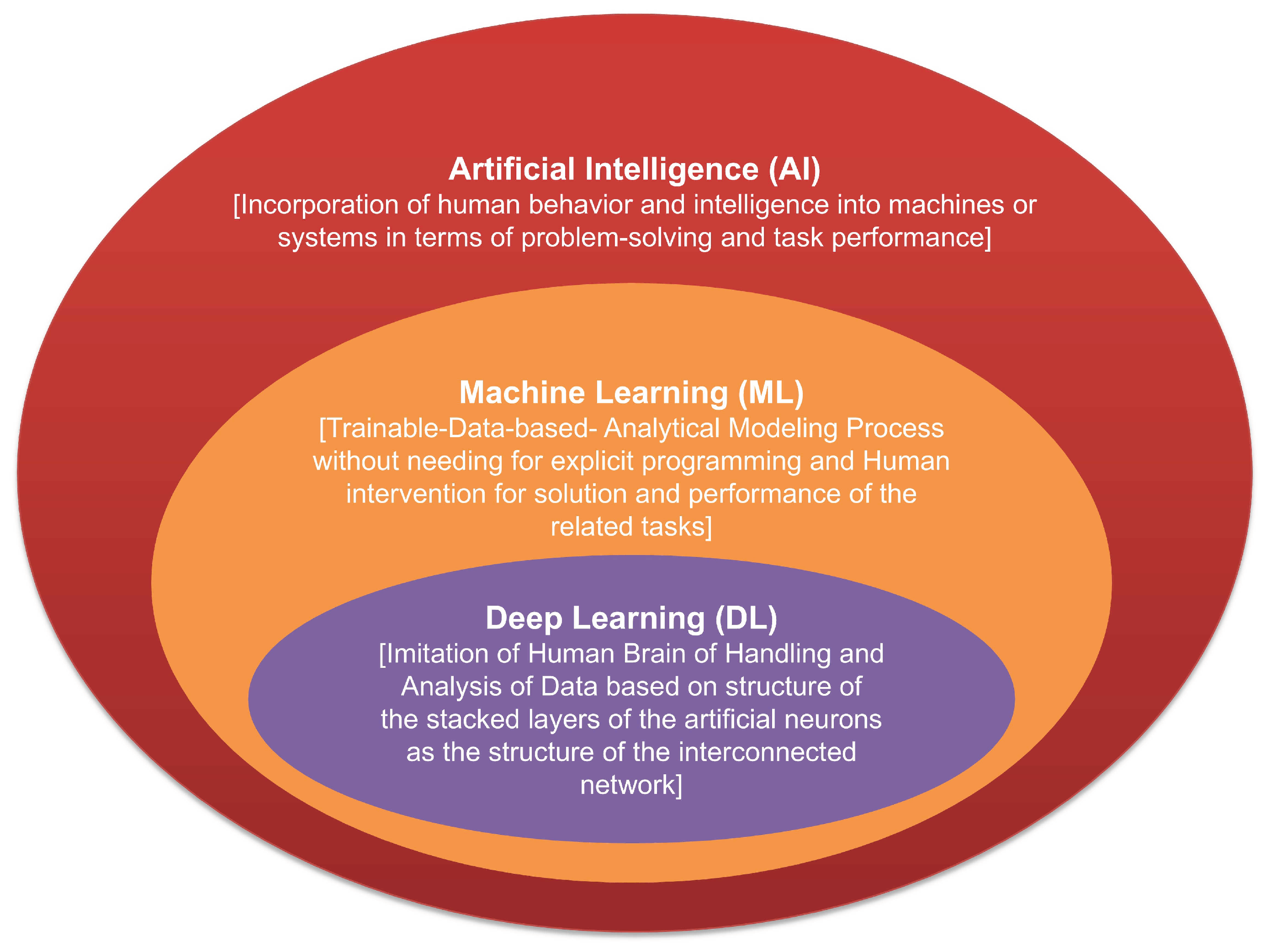
Figure 3.
Example of RP of time series.
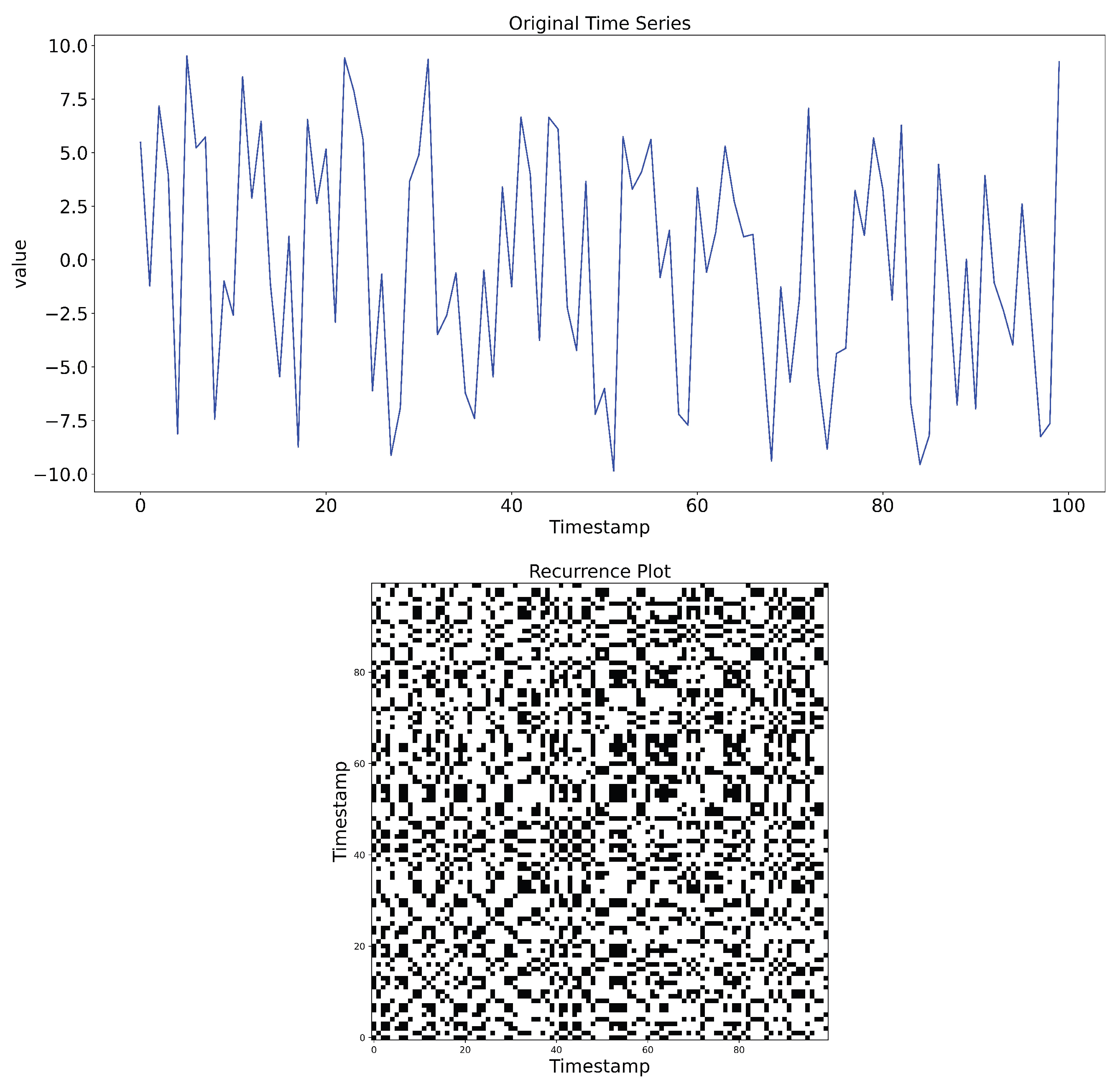
Figure 4.
Example of RP of time series.
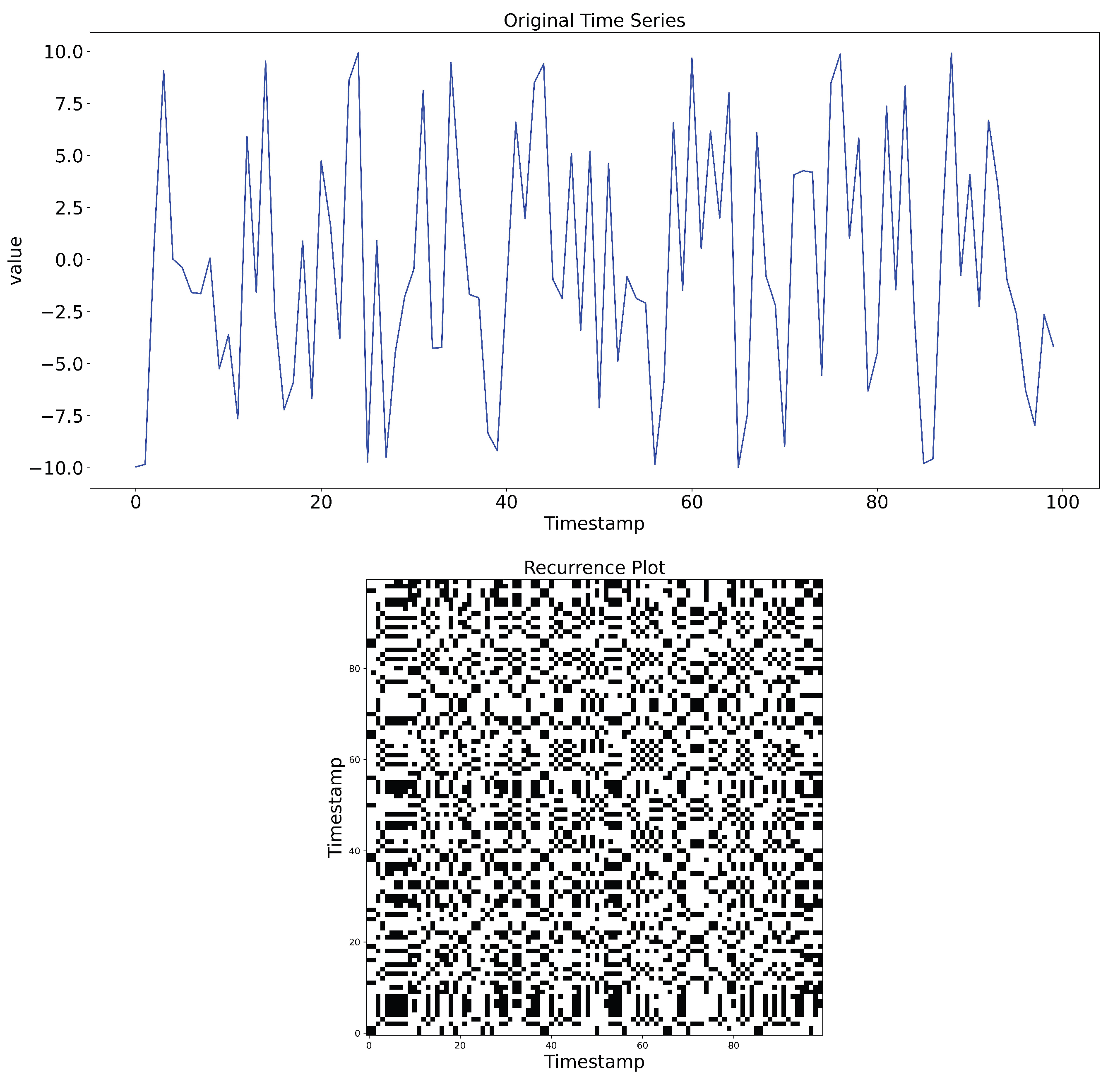
Figure 5.
Workflow for encoding raw time-series data as images using GAF technique.
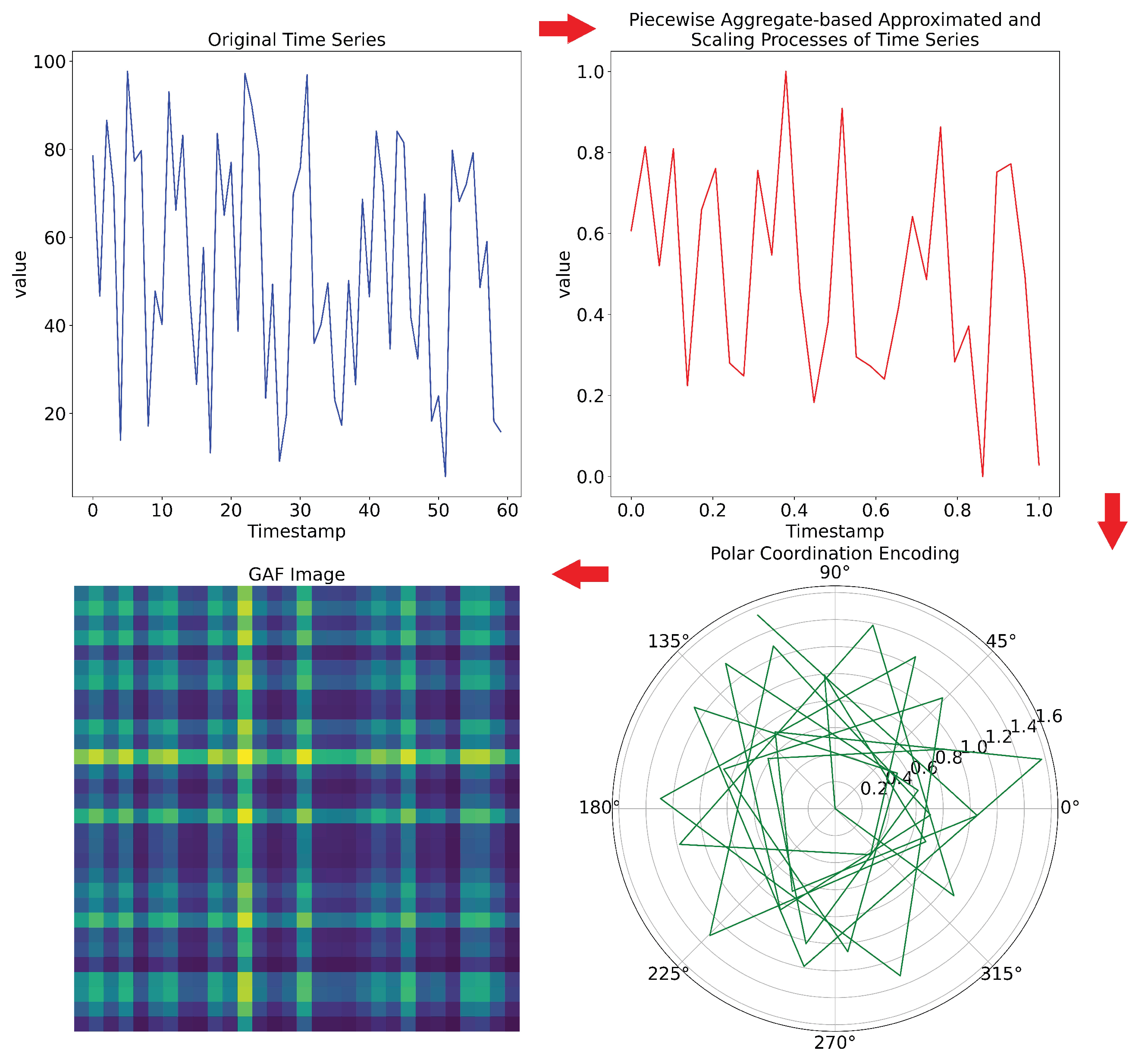
Figure 6.
Example time-series signal (top); images of GASF and GADF matrix transformation (bottom).
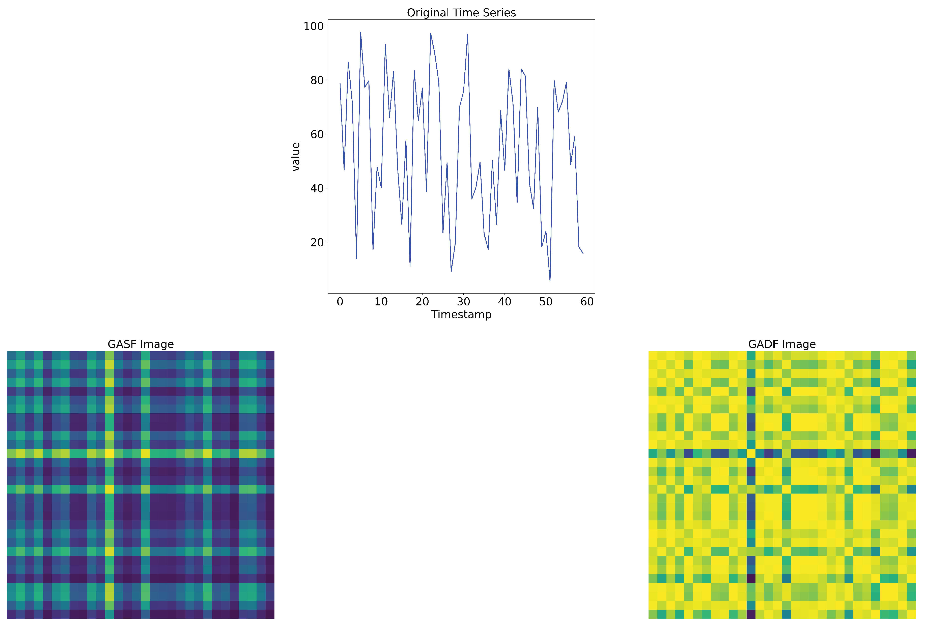
Figure 7.
Workflow for encoding raw time-series data as images using MTF technique.
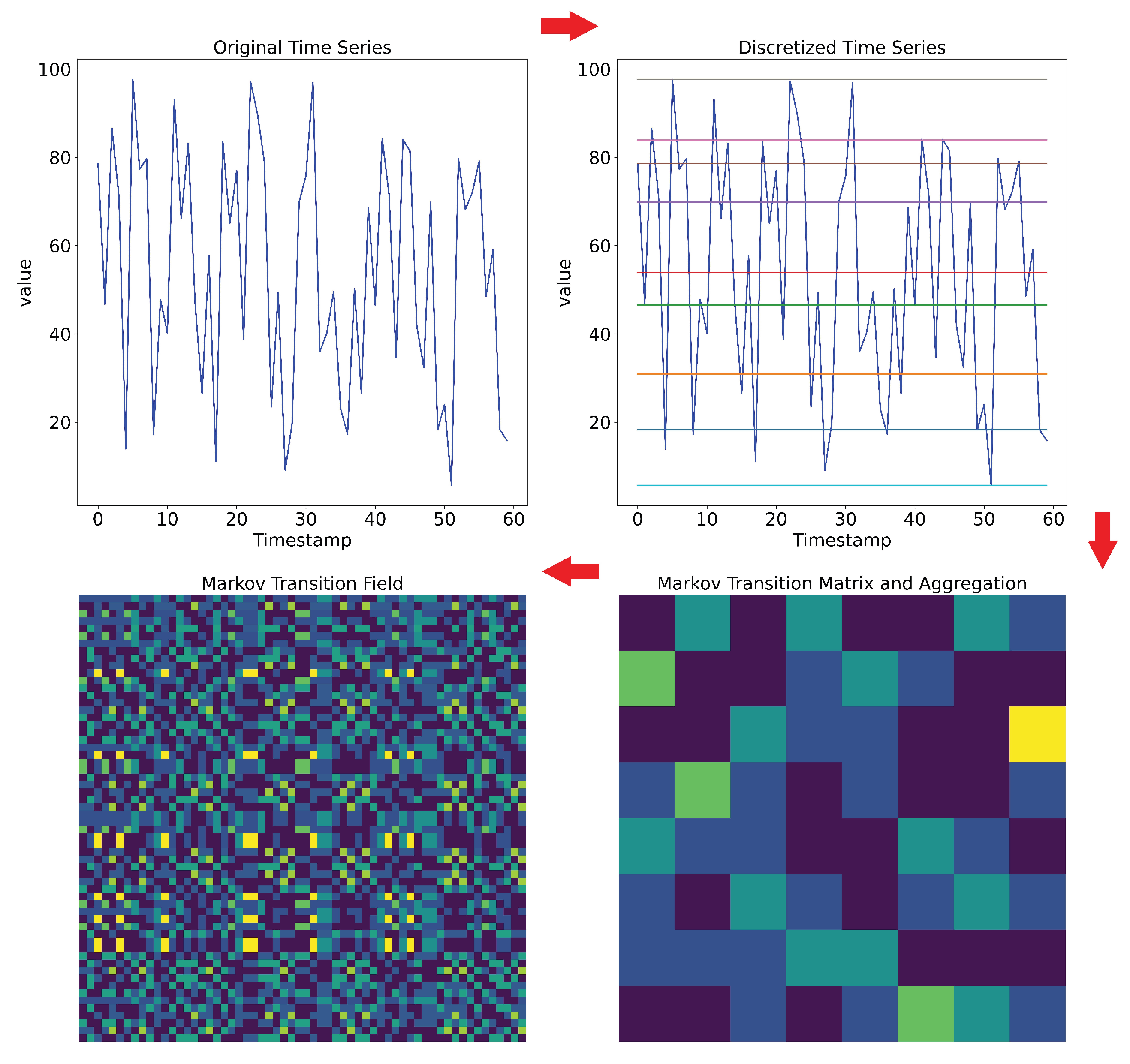
Figure 8.
LeNet-5 architecture [32].
Figure 8.
LeNet-5 architecture [32].
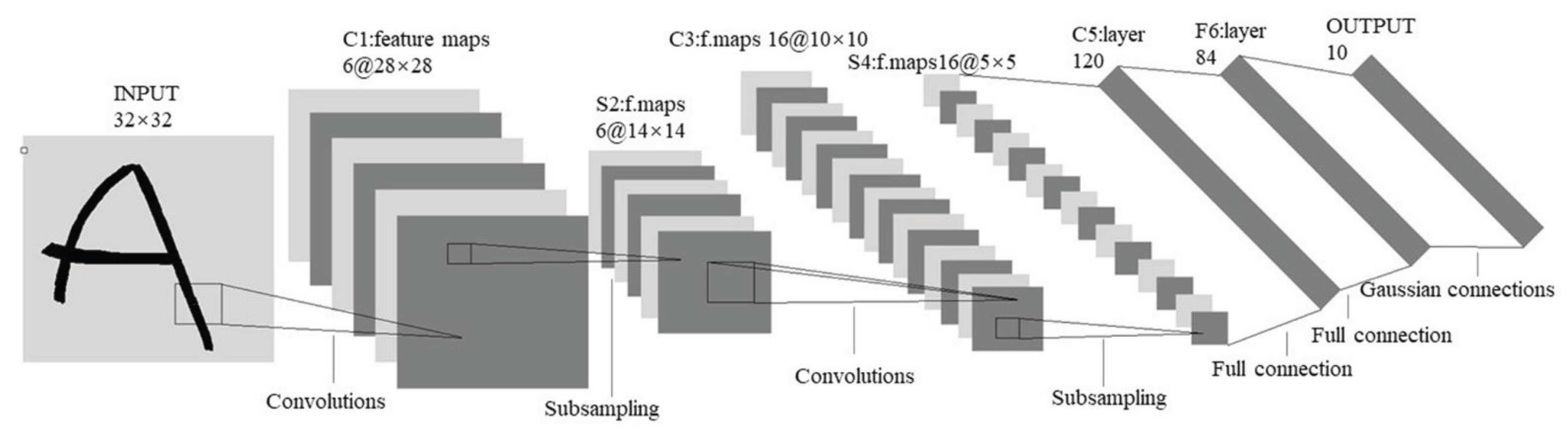
Figure 9.
General structure of CNN.
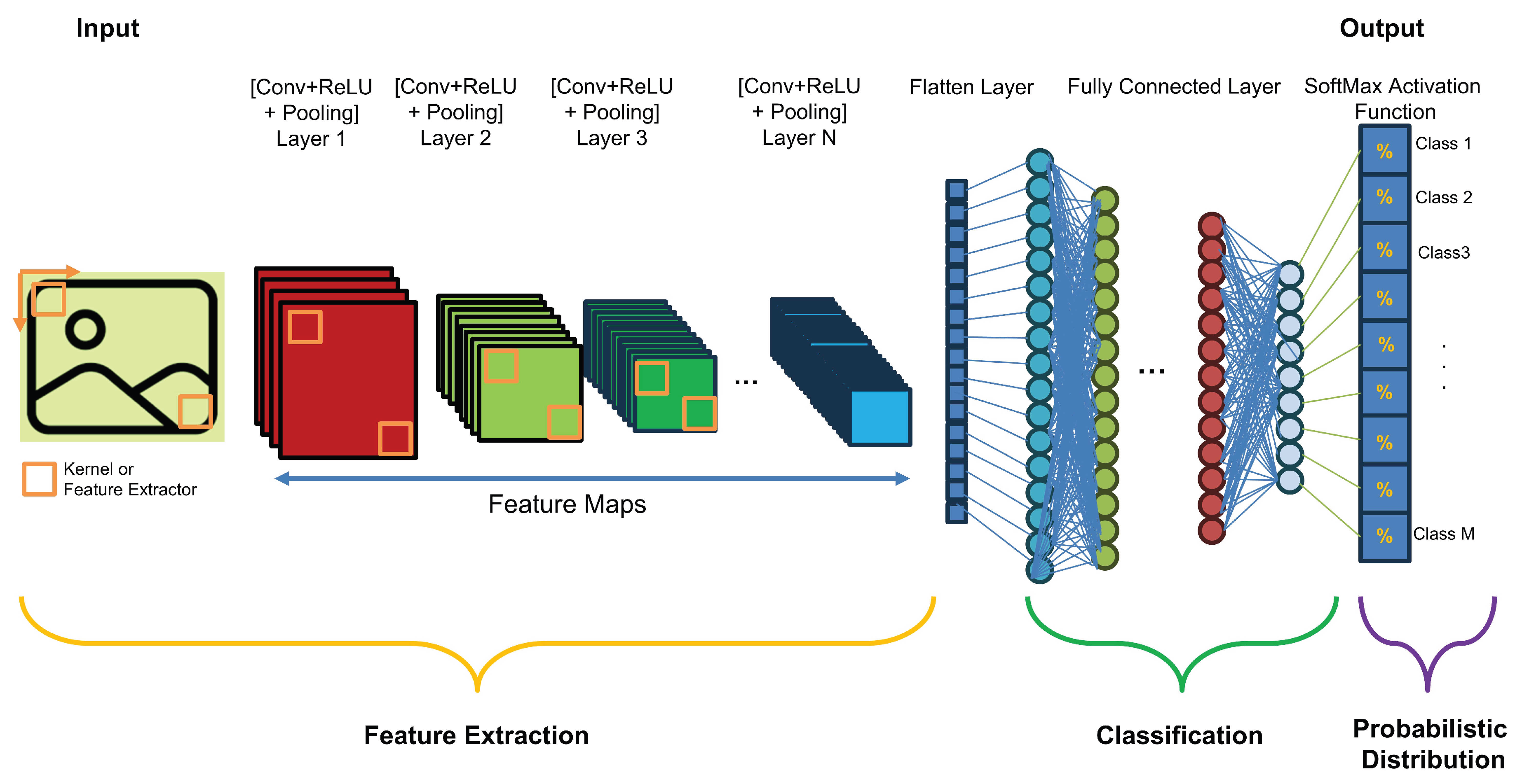
Figure 10.
Workflow of the benchmarking transfer learning strategy for time-series imaging proposed in [1].
Figure 10.
Workflow of the benchmarking transfer learning strategy for time-series imaging proposed in [1].
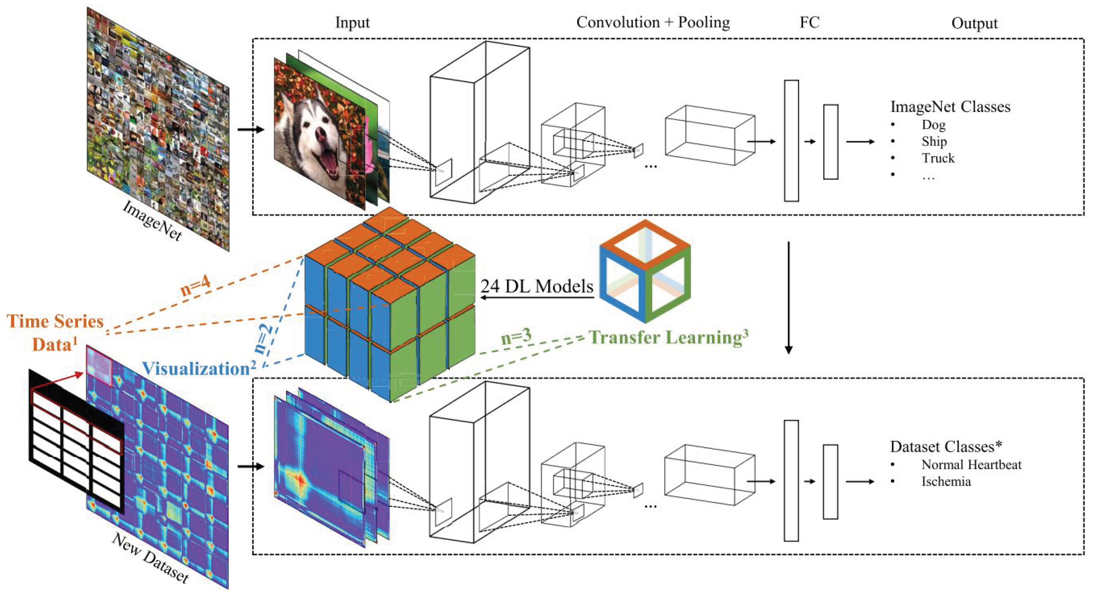
Figure 11.
Classification system of time series proposed in [21].
Figure 11.
Classification system of time series proposed in [21].
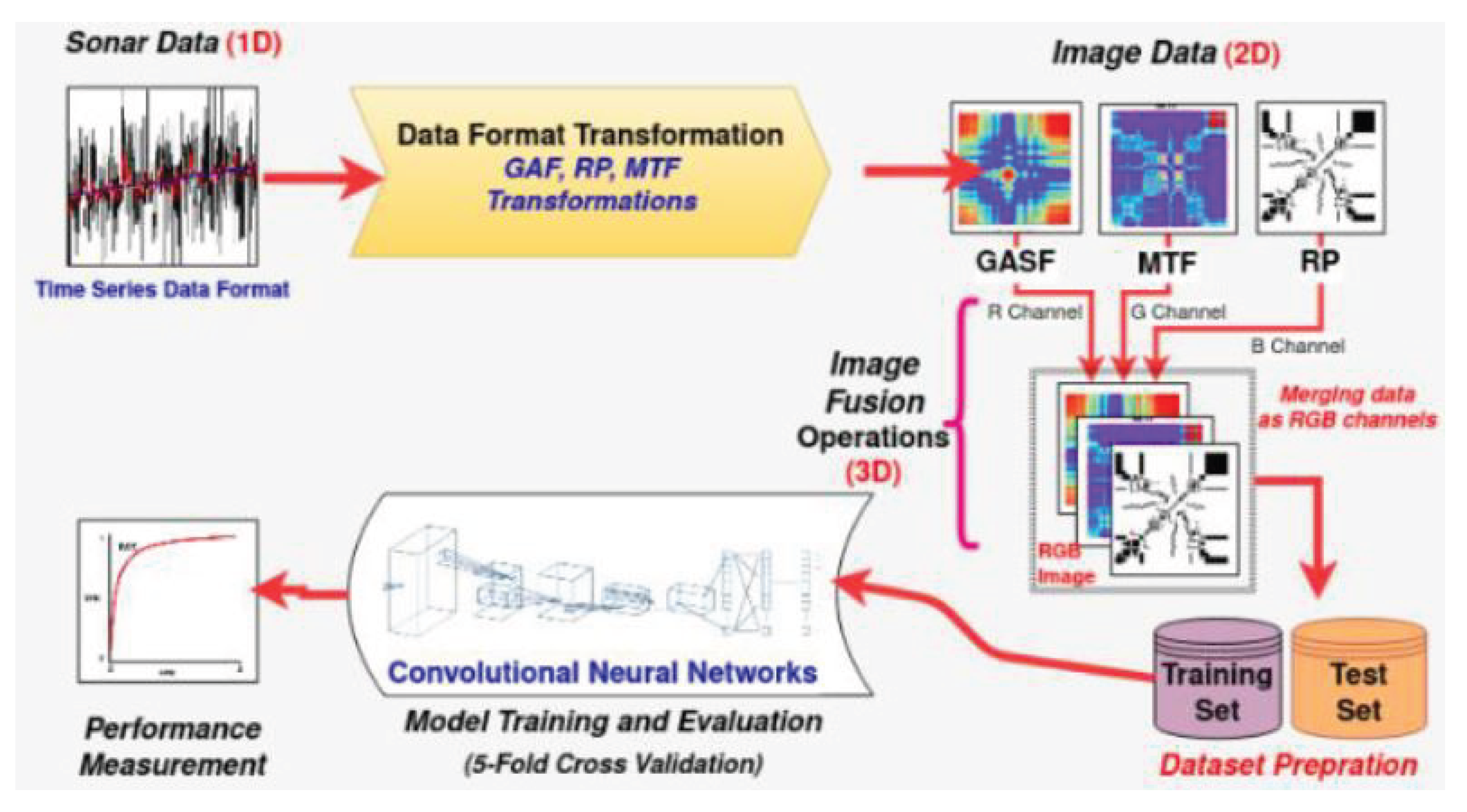
Figure 12.
CNN architecture of the proposed classification system of time series proposed in [21].
Figure 12.
CNN architecture of the proposed classification system of time series proposed in [21].
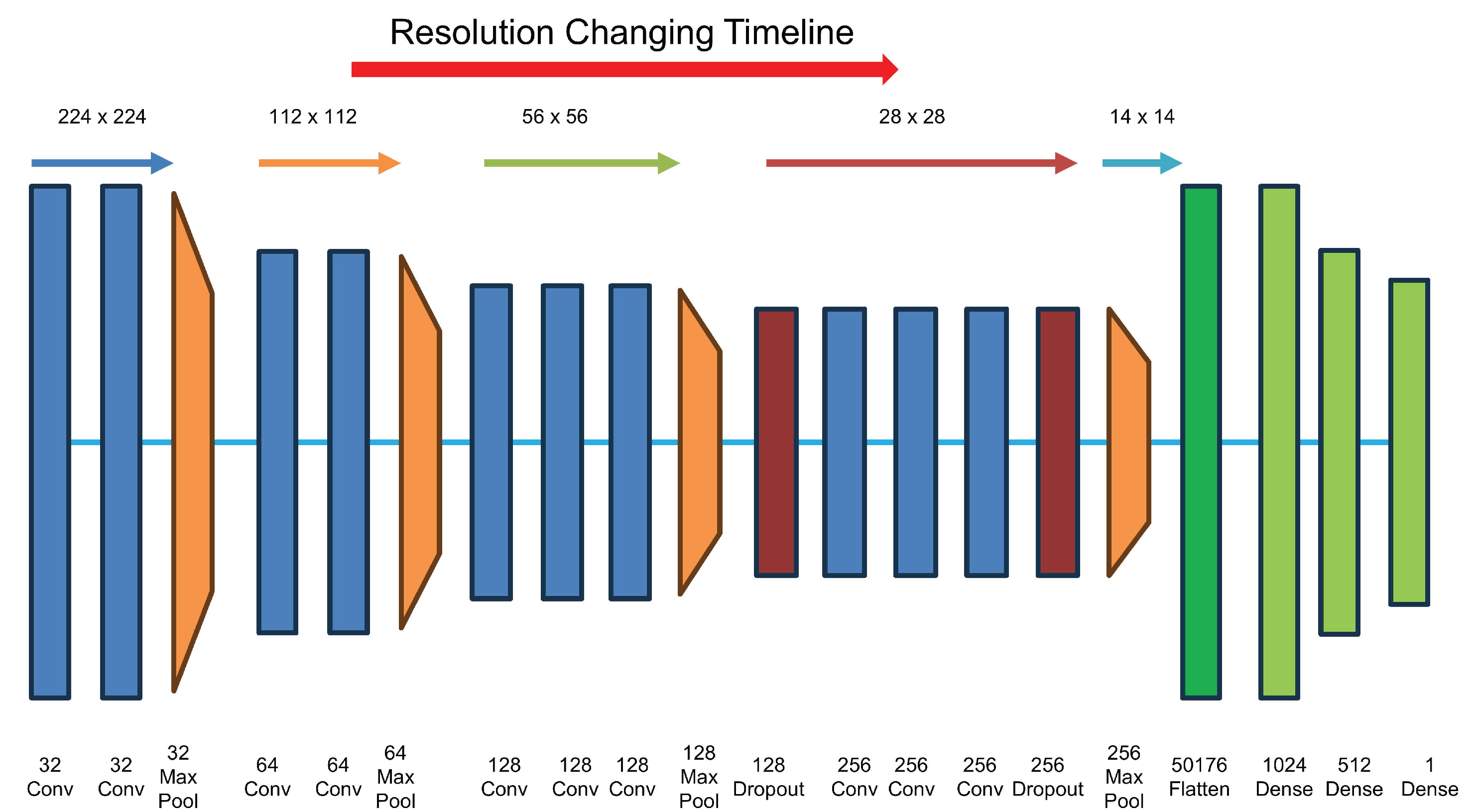
Figure 13.
“Fingerprint” term in the context of the G3FI technique: Original time series of the two states (top); related G3FI images (bottom).
Figure 13.
“Fingerprint” term in the context of the G3FI technique: Original time series of the two states (top); related G3FI images (bottom).

Figure 14.
Results of time-series imaging: Original time series consisting of 60 descriptive features/variables (top); related transformed images of the RP, GAF and MTF and G3FI techniques (bottom).
Figure 14.
Results of time-series imaging: Original time series consisting of 60 descriptive features/variables (top); related transformed images of the RP, GAF and MTF and G3FI techniques (bottom).
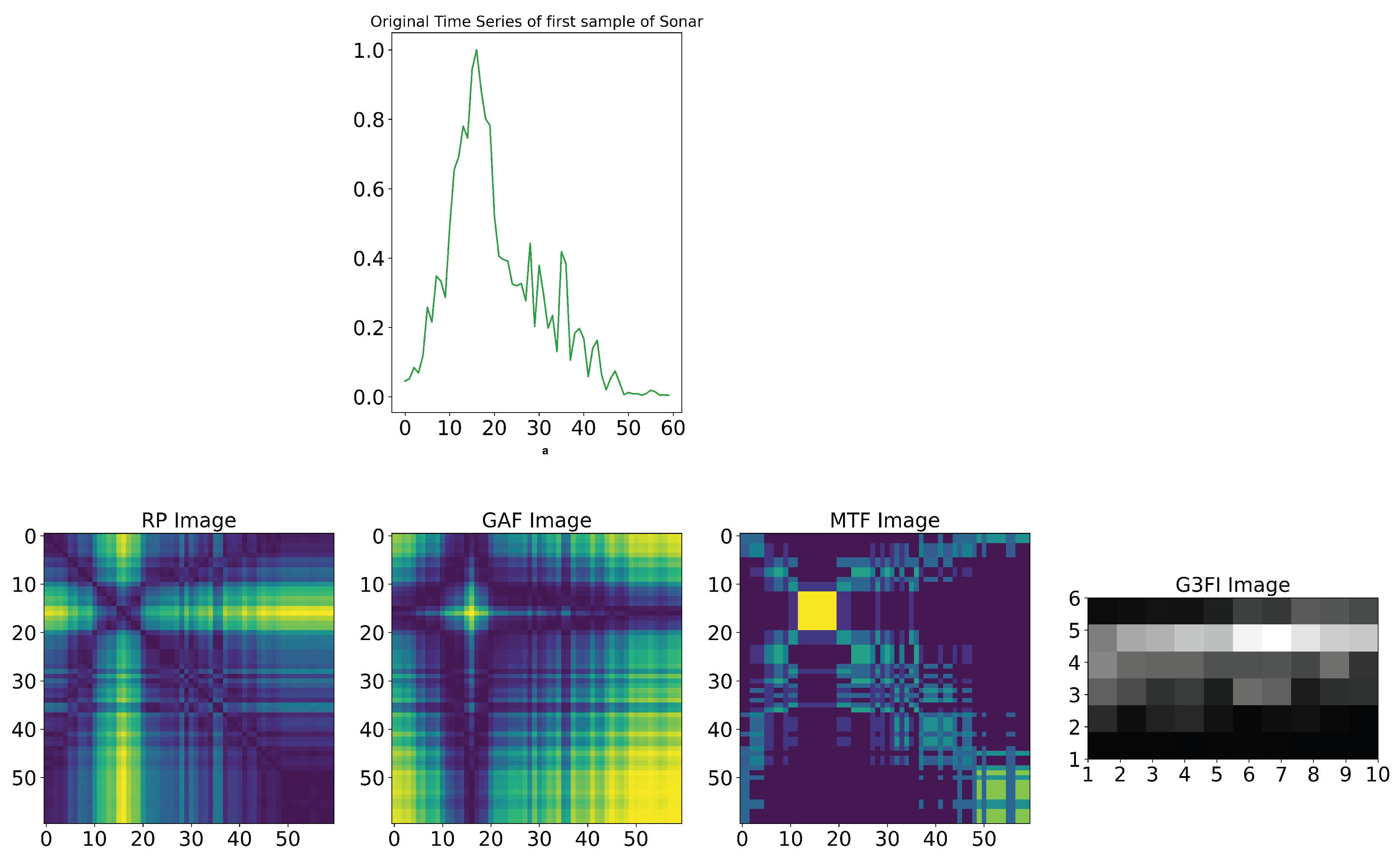
Figure 15.
Architecture of the proposed classification system for time series encoded using the G3FI technique.
Figure 15.
Architecture of the proposed classification system for time series encoded using the G3FI technique.
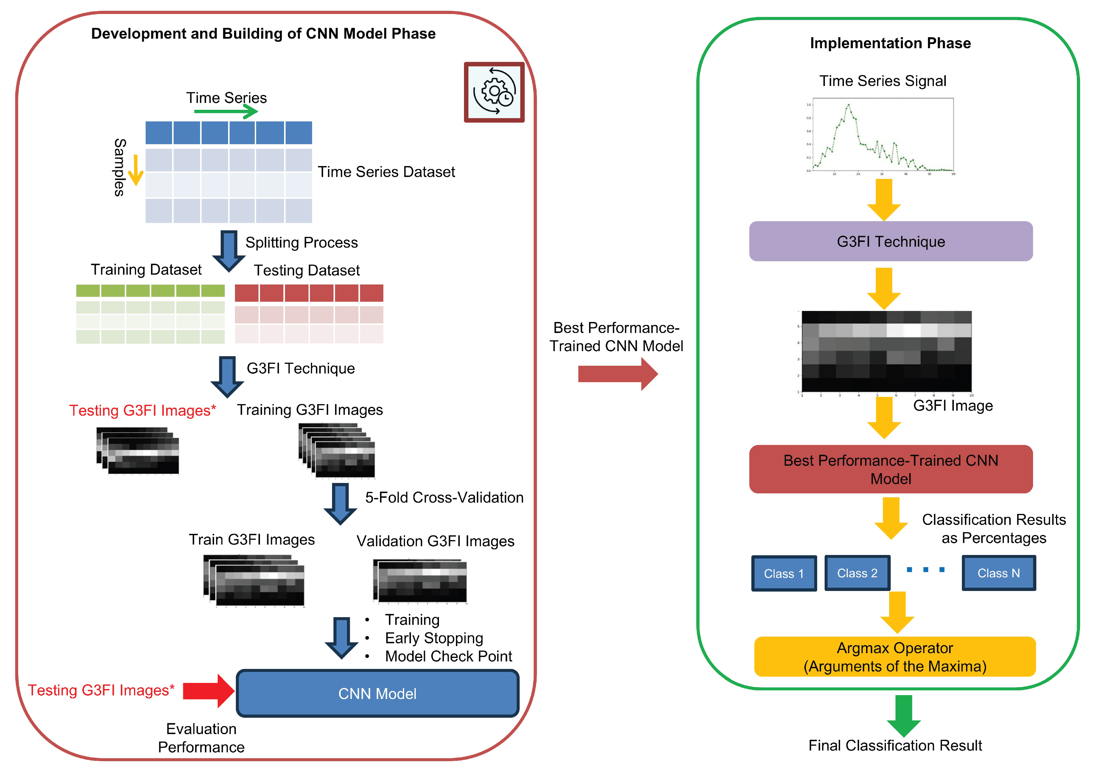
Figure 16.
Structure of the CNN model used in the proposed G3FI-Image-Encoded-Time-Series-CNN-based Classification System. Legend: Conv—Convolutional Layer with a filter size of , MaxPool—Maximum Pooling Layer with a window size , Flatten— Flattening Layer, FC—Fully Connected Layer, Sigmoid—Sigmoid Output Layer
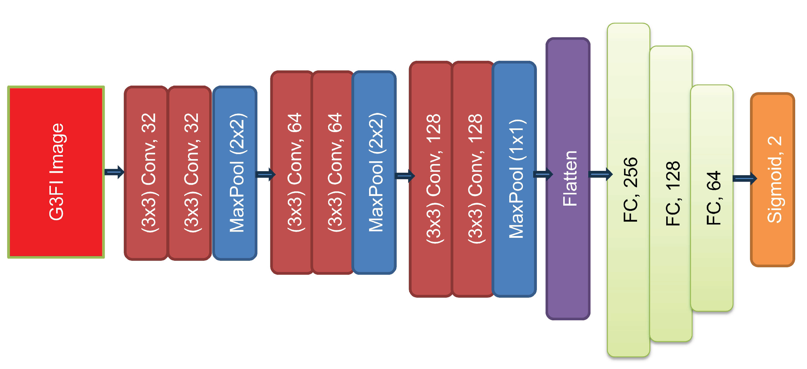

Table 1.
Overview of datasets used in [1].
Table 1.
Overview of datasets used in [1].
| Dataset | Number of Samples | Length of Time Series | Classes |
|---|---|---|---|
| Computers | 500 | 720 | 1: Desktop, 2: Laptop |
| DodgerLoopGame | 158 | 288 | 1: Normal Day, 2: Game Day |
| ECG200 | 200 | 96 | 1: Normal, 2: Ischemia |
| AbnormalHeartbeat | 606 | 3053 | 1: Normal, 2: Arrhythmias |
Table 2.
Overview of the total number of the parameters of trained proposed G3FI-CNN model.
| Dataset | Total number of the parameters of trained G3FI-CNN model |
|---|---|
| AbnormalHeartbeat | 5,866,658 |
| Computers | 1,705,122 |
| DodgerLoopGame | 853,154 |
| ECG200 | 525,474 |
| Sonar | 394,402 |
Table 3.
Comparison of performance of the G3FI-image-encoded time-series-CNN-based classification system to those in the considered related works.
Table 3.
Comparison of performance of the G3FI-image-encoded time-series-CNN-based classification system to those in the considered related works.
| Name of Dataset | Gross et al. [1] | Buz et al. [21] | Our System |
|---|---|---|---|
| Computers | 74.4% | – | 71.8% |
| DodgerLoopGame | 93.7% | – | 93.4% |
| AbnormalHeartbeat | 66.5% | – | 73.1% |
| ECG200 | 86.5% | – | 94.9% |
| Sonar | – | 97.6% | 98.5% |
Disclaimer/Publisher’s Note: The statements, opinions and data contained in all publications are solely those of the individual author(s) and contributor(s) and not of MDPI and/or the editor(s). MDPI and/or the editor(s) disclaim responsibility for any injury to people or property resulting from any ideas, methods, instructions or products referred to in the content. |
© 2025 by the authors. Licensee MDPI, Basel, Switzerland. This article is an open access article distributed under the terms and conditions of the Creative Commons Attribution (CC BY) license (http://creativecommons.org/licenses/by/4.0/).
Copyright: This open access article is published under a Creative Commons CC BY 4.0 license, which permit the free download, distribution, and reuse, provided that the author and preprint are cited in any reuse.


