Submitted:
20 September 2025
Posted:
22 September 2025
You are already at the latest version
Abstract
A combinatorial tree \( (Pt) \) is used to record valid colors to be assigned to each of the vertices of a planar graph \( G \) of order \( n \). The main process consists of a loop that incrementally builds \( G \) vertex by vertex, starting from the most internal triangular face of \( G \), and in \( n-3 \) iterations, the paths constructed in \( Pt \) will have the valid color labels assigned to the vertices of \( G \). This method ultimately generates all proper 4-colorings of \( G \). In each iteration, a vertex \( v_i \in V(G) \) is selected to be aggregated to the current induced subgraph \( G_i \) of \( G \). This process, alongside the use of the \( Pt \) tree (which results in a binary tree of depth \( n-3 \)), ensures all proper 4-colorings of \( G \), regardless of the topology of the maximal planar graph \( G \). Additionally, we develop an existential theorem that shows that for any maximal planar graph \( G \), it is always possible to create a proper 4-coloring. Furthermore, we detail a method through which such a 4-coloring can be constructed. Also, we present the extremal topologies of planar graphs, highlighting those with the maximum and minimum number of 4-coloring functions.
Keywords:
4-coloring problem
; existence theorem 4-coloring
; maximal planar graph
; vertex building graph
; combinatorial tree
1. Introduction
The graph vertex coloring problem involves assigning colors to the vertices of a graph with the aim of using the fewest possible colors, while ensuring that adjacent vertices have different colors. The minimum number of colors required in any such coloring of a graph G is known as the chromatic number of G, denoted by . If it is possible to color G using a set of k colors, then G is said to be k-colorable, and such a coloring is referred to as a k-coloring. When , then G is described as k-chromatic, and any k-coloring represents a minimum coloring of G.
Since its initial proposal in 1852 by Francis Guthrie [7], a conjecture was proposed to know if it is possible to use a maximum of 4 colors for map coloring, in such a way that no two adjacent regions of the map share the same color (The Four Color Conjecture ’4CC´). This conjecture has presented a significant challenge to the scientific community for constructing a mathematical proof to validate it.
The famous Four-Color Theorem (4CT) states that every planar graph is vertex 4-colorable [18]. However, the 4CT could involve the 3-coloring problem, which is a classic NP-complete problem, even for planar graphs [11]. The 4CT settles a conjecture that has been for more than a century, the most famous unsolved problem in graph theory and perhaps in all of mathematics [10]. The 4CC is now, a broad area of research, with hundreds of contributors and thousands of contributions [3]
A proof of the 4CT proposed by Kempe [12] in 1879, turned out to be flawed. The seeming impossibility of proving the 4CT, and the increasing power of computers in the early 1960’s, led scientists to use computers for showing that there are no counter-examples for the 4CT. A programming proof of the 4CT was introduced in 1977 by Appel and Haken [1,2], assisted in algorithmic work by Koch [2].
The orientation in resolving the 4CT, based on Appel and Haken’s algorithm [1,2], is based on the application of the discharging method plus a large finite case check by computer. Initially, this involved analysing 1,834 configurations in order to identify all possible unavoidable sets of configurations in a planar graph. Robertson [18] has narrowed down the number of unavoidable sets of configurations to close to 700. However, this reduction requires significant computational support to manage the numerous cases that can be created for any planar graph. As a result, this computer program becomes impractical to present as a mathematical proof of the 4CT.
Initially, the proof did not gain general approval among mathematicians, however, it did fuel a debate [19] on the meaning of a mathematical proof. Nonetheless, a variation of the initial programming proof of the 4CT published in 1997 by Robertson, Sanders, Seymour, and Thomas [18] has been predominantly accepted.
The discharging method has proven to be an effective proof technique, particularly for graph coloring problems. However, its main drawback is that it often necessitates extensive case analysis. To address this challenge, various automatic methods have been developed to search for discharging proofs automatically [4,6].
For example, in 2005, Gonthier [9] applied an automatic theorem software (the Coq proof assistant) to build an automatic proof for the 4CT. The computer-assisted proofs contributed significantly to the development of "computer formal methods as a primary proof technique." For instance, in the 4-coloring problem, these methods enabled the mathematical argument to be verified more thoroughly, with various cases encoded and checked by an automatic proof assistant. For a comprehensive history of the four-color problem and in-depth review of plane graph 3- and 4-colorings, refer to Fritsch and Fritsch [7] and to Borodin [3].
Additionally, there are numerous publications available online focused on the ’proof’ of the 4CT theorem. However, to date, none of these have been acknowledged by researchers in the field as a formal, complete, and correct proof of the 4CT.
We address the 4CT problem from a combinatorial perspective, through the vertex incremental construction of a maximal planar input graph G. Our method utilizes a binary tree to list the valid colors of the vertices of G. This article also provides a clear and novel demonstration of the 4CT by using graph theory and combinatorial techniques, all without the assistance of a computer program.
This paper is structured as follows: the introduction section 1 provides a general introduction about the 4 coloring theorem. Basic definitions and the notation to be used are presented in section 2 - Preliminaries. In section 3, we introduce extremal topologies of planar graphs for the 4-coloring problem. In section 4, the main structures and procedures to be used in our method are introduced. In section 5, the existence’ theorem for the 4CT is proved. The final section offers conclusions drawn from this work.
2. Preliminaries
Let us consider a planar graph , where and in the case of planar graphs, let be the number of faces in G. We assume that the reader is acquainted with common terms and symbols related to graph theory, specifically concerning planar graphs (see e.g. [10] and [17]). In this section, we will introduce only a few notation that will be utilized.
When two distinct vertices are connected by an edge , we describe v and w as adjacent vertices. A graph where every pair of different vertices is adjacent is termed a complete graph. The complete graph with n vertices is symbolized as .
The set , defined as the neighborhood of x in a graph G, is given by , while its closed neighborhood, denoted , is the union of with , i.e., . The size or cardinality of a set A is the number of elements of A, denoted by . The degree of a vertex , denoted by , is . Only when there is no doubt about the graph G to which the vertex’s neighborhood refers is it omitted. The degree of the graph is denoted as .
A subgraph of a graph , is also a graph where and . When the subgraph contains all the vertices from G, is a spanning subgraph of G, and is termed as induced by , if it includes all edges from G connecting the vertices of . Such an induced subgraph is also denoted as . Then, would be the induced subgraph from . On the other hand, when , . When and , previous notation is usually simplified as and , respectively.
2.1. Elements of a Planar Graph
A graph drawing of a graph G, denoted as , represents each vertex as a unique point in the plane, and each edge as a simple Jordan arc with endpoints and . A drawing is considered planar if it can be embedded in a plane without any two edges intersecting, except possibly at their shared endpoints. When a graph G has a planar drawing, it is called a planar graph.
One relevant result in graph theory is Kuratowski’s theorem, which provides constraints for determining whether a graph G is planar. According to this theorem, G is planar when it does not contain a subgraph that is a subdivision of or [13]. It is worth mentioning that a disconnected graph is planar if and only if each of its connected components is planar. Similarly, the theorem of Wagner states that a graph G is planar if and only if it does not have or as minor [15].
Planar graphs are significant in both graph theory and graph drawing. They possess several interesting properties: they are sparse, four-colorable, and their structure is described succinctly and elegantly [5].
A planar graph drawing divides the plane into connected areas known as faces. The face that extends infinitely is referred to as the outer face or the external face of the graph. denotes the outer face of a given planar graph G. Meanwhile, will denote the outer face for the graph .
If all the vertices of a planar graph can be drawn incident to the outer face of the graph, then it is called an outerplanar graph. Similarly, an outerplanar graph may be characterized by the two forbidden minors and .
Let be the set of closed non-intersected faces of G. The internal area of each face is delineated by the set of edges that enclose it. Notice that the outer face of the graph is not included in , because we want to consider only the internal faces related to G. denotes the internal vertices of G, which are vertices not incident to , i.e. . Let , a facial walkw corresponding to f is the shortest closed walk induced by all edges incident with f. If the boundary of f is a cycle, the walk is called a facial cycle. The length of a face f is denoted by and equals . We say that a face is a triangle when .
Two faces and in are considered adjacent if they share edges, meaning . If two faces do not share any edges, they are termed independent faces. It is worth noting that independent faces may share vertices but do not share edges. A collection of faces is independent if every pair of faces within it is independent. An edge in G that is not part of a facial cycle of any internal face in , is called an acyclic edge. An acyclic edge is considered adjacent to a face if it shares only one vertex. Similarly, two acyclic edges are adjacent if they have a common endpoint.
Given a planar drawing, the (clockwise) circular order of the edges incident to each vertex is fixed. Two planar drawings are equivalent if they determine the same circular orderings of the edges incident to each vertex (sometimes called rotation scheme). A (planar) embedding is an equivalent class of planar drawings and is described by the clockwise circular order of the edges incident to each vertex. A graph put together with one of its planar embedding is sometimes referred to as a plane graph [5].
3. Determination of Extremal Topologies for the 4-Coloring
Let be a set containing 4 different colors. Given a planar graph , let be the assigning 4-colouring function which assigns to each vertex an unique colour in . The assigning function c is proper if for each edge , . Given a planar graph , we analyse in this section, the set of all possible 4-coloring functions that can be built on .
We consider that exist an arbitrary ordering on the set vertex from G, i.e. . Let H be a subgraph from G, denotes a proper 4-coloring on the set vertex from H and inferred by the ordering on V. For example, given an arbitrary edge , , where , and , if , otherwise . denotes a total 4-coloring of G according to the order given on the set vertex from G.
Let be the set of all proper 4-colouring that can be built on a graph G. And let be the number of different proper 4-colorings that can be built on the graph G.
3.1. Counting 4-Colouring Process
We introduce a systematic way to count all 4-coloring of any subgraph , induced by the ordering set vertex from V. In order to calculate , we consider that each vertex and each edge from H is visited only once.
The first visited vertex would consider 4 different colors since it has not any restriction for assigning one element from . When the following vertices are considered, they could have restriction according to the previous visited vertices from its neighbourhood.
For example, for an isle vertex u, . Given an aisled unitary edge , , since when v is visited, it has only one restricted color, the color of u.
Let us consider the planar graph formed by n vertices, where each vertex is an isle, , , and . Then, is a completely disconnected graph. In this case, each vertex could be colored with whatever of the four colors, since there is not constraint between colors for any pair of vertices, then . consists of all lists of n items formed by the colors in the set . There are different 4-colorings for .
An edge constraints the combination of colors that can be assigned to its extreme points. In the case of the 4-colorings, and only one edge e, although can be assigned one of the four colors from , for each color assigned to , can only be assigned 3 possible colors. , and therefore, .
In fact, when a path (with n edges and vertices) is considered, the previous numeric formula is kept. We are traversing on linearly, beginning from vertex . To the first vertex visited , it can be assigned whatever color from . But for each new vertex visited , it has three possible colors to be assigned, avoiding the use of the color from its previous neighbour (See Figure 1). Then, it follows that .
When a tree is traversed in post-order, after visiting the root node , the following vertices to be considered have only one restricted color. Considering a connected planar graph, a similar formula for the number of 4-colorings is shared for any tree graph with n vertices and edges (see for example, Figure 2). But for other topologies, the vertices can take more than one restricted color.
Lemma 1.
The connected planar graph with a maximum number of 4-colorings is a tree.
Proof.
Let be a tree of order n, whose root vertex is . is traversed in pre-order, then is the first vertex visited. can take one of the 4 possible colors from .
For any node where , when is visited during the traversal, it has one unique restriction: it cannot be colored with the same color as its already-visited parent node. Therefore, has three possible colors available for use. As a result, the formula for the total number of colorings is given by .
A tree represents the topology of a graph with the minimum number of edges required to keep it connected to any planar graph containing n vertices. Therefore, the maximum number of distinct 4-colorings for any connected planar graph with n vertices is given by . □
When new edges are added to a connected planar graph without adding any new vertices, the number of possible 4-coloring functions decreases. This is because the additional edges place constraints on the colors that can be assigned to the vertices at their endpoints.
When acyclic edges are added to a connected planar graph G, it necessitates the addition of new vertices. As a result, the number of valid 4-coloring functions increases. This is because each new vertex contributes to a threefold increase in the previous value of .
In a planar graph, the acyclic subgraphs are 4-colorable and, in fact, they are 2-colorable. To simplify the counting process for 4-coloring planar graphs, we will assume from now on that any input planar graph G does not contain any acyclic edges. Consequently, all faces in G will have a facial cycle.
For example, consider simple cycles such as the triangle and the square. In Figure 3 and Figure 4, we show the combinatorial enumeration of the all 4-coloring functions created for both cycles.
It is not complicated to count 4-colorings in the case of simple cycles. For instance, consider a triangular cycle . The first vertex can be assigned one of the 4 colors. The second vertex can choose from only 3 colors, as it cannot use the same color as . Finally, the third vertex is left with only 2 available colors. Therefore, the total number of 4-colorings for a triangular face can be calculated as (see Figure 3).
In the case of even cycles, such as a square , we can assign colors to the vertices as follows:
- The first vertex, , can be assigned one of 4 colors.
- The second vertex, , has only 3 color options since it cannot repeat the color of .
- The third vertex, , can also be assigned one of 3 colors, provided it is different from the color of . However, two of these choices for limit the available color options for to 2 colors. This is because cannot have the same color as or if they are different. While one of the colors of can have 3 colors assigned for .
Thus, the total number of 4-colorings for a square cycle is . In Figure 4, only one of the 4 branches derived from assigning the color (out of the 4 possible colors) to vertex is shown.
Perhaps the most renowned property for planar graphs is the one stated by Euler’s theorem, which states that planar graphs are sparse. Namely, given a plane graph with n vertices, m edges, and f faces, planar graphs hold .
A direct consequence of Euler’s formula is that in a maximal planar graph (where every face is a triangle) with at least three vertices, we have , and then . This number reduces to for maximal outerplanar graphs with at least three vertices (and for general outerplanar graphs). Furthermore, when the planar graph is triangle-free, then . Finally, if the graph is a tree, then .
The previous insights enable us to substitute m with n in asymptotic calculations concerning planar graphs, whereas for general graphs, we can only assume that . From a practical standpoint, this enables us to determine the non-planarity of denser graphs without examining all edges, which would necessitate a quadratic-time algorithm.
On the other hand, relating to 4-coloring functions on planar graphs, it is known that any general planar graph G can be reduced to a maximal planar graph and where all 4-coloring for is also a 4-coloring for G.
Considering maximal planar graphs, the bound can be substituted for relating number of faces with number of vertices, and the Euler’s equality holds , obtaining . Considering maximal planar graphs, and tabulating the maximum value for the number of edges and number of faces while the number of vertices is increased one by one, the Table 1 is obtained.
Let be a maximal planar graph of order n. We consider a subgraph , which is induced from G and formed by , where is the most internal triangular face in G.
According to Figure 3, we have . However, when we fix the first three colors for the vertices of , the factor simplifies to 1. This simplification avoids the need to consider the possible permutations of the vertex colors in .
Table 1 shows that when a planar graph grows incrementally, one vertex at a time, the addition of a new vertex to the current subgraph, i.e. , at this point, the maximum number of edges that can be incident from to is three, and since maintains the maximum number of edges for each new vertex added to it.
Since for each , the size of its outer face remains constant at three (denoted as ), we can ensure that in each iteration, when a new vertex is incorporated into , the maximum number of new edges continues to form. This process results in an extreme topology for planar graphs where G has a minimum number of 4-coloring functions.
Lemma 2.
The planar graph with a minimum number of 4-colorings is the graph formed by the nesting of .
Proof.
Let be a planar graph that has been formed iteratively and incrementally, beginning from the triangle face , which is the innermost face of . Let . From example 1, we know that . Although if we fix the three different colors for the endpoints of , we reduce the factorial number of permutations on , and simplify the number of colours to be assigned to the following vertices to be aggregated.
As is formed by adding vertex by vertex, starting with , and in each iteration i, a new vertex is added, then . We want that each time that the new vertex is aggregated to , the change in the value of to has a minimal increase. The minimum growth of the function occurs when . This situation arises when is incident with exactly three different colors from the outer face of .
In order to use a minimum number of edges for , at least . And in this case, has just only one possible color to be assigned, then .
Observe that (see Figure 5) forms a nested pattern created by aggregating each new vertex to the current graph. □
Figure 5 illustrates an extreme planar graph with the minimum number of 4-coloring functions. By fixing the colors of the first triangular face , the colors assigned to the vertices alternate between only two possible colors. In this way, has only one option of colours for its vertices. However, the factorial number of permutations appears when no color is fixed to the initial triangle . Thus, considering the general case, .
Only in the case that is incident to the 4 different colors in , it follows that for this combination of colors on , it is not possible to assign a color from to . However, in the following sections, we will show that there is no planar graph G for which .
4. Principal Procedures and Structures
In the process of constructing a 4-coloring for an input planar graph , useful preprocessing involves transferring certain elements to a Stack. This includes both vertices of degree less than 3 and acyclic edges, following an iterative order that starts with the objects of the lowest degree. By doing so, we obtain a simplified graph G from . The elements in the stack can then be 4-colored without difficulty after 4-coloring the remaining graph G.
Additionally, it is beneficial to reduce the remaining graph to one of its maximal versions, where all internal face of G are triangles. Although our proposal can work on non-maximal graphs, the analysis of the method is simplified by considering only triangle as internal faces. As it is known, if an input graph is not maximal, this can be polynomially reduced to a maximal graph G, where any 4-coloring of G is also a 4-coloring for . Therefore, in this section, we will focus on processing a maximal connected planar graph G, in which all vertices have a degree greater than 2.
During the counting of 4-colouring functions, it is not necessary traversing the vertices and edges in a specific order. However, all object (vertices and edges) have to be considered during the counting of 4-colourings.
As it is known, an arbitrary ordering on the vertex set does not help to reduce the computational complexity of graph problems. Furthermore, imposing an arbitrary vertex ordering does not change the NP-hard status, because the hardness of a graph problem arises from the combinatorial structure of the graph, not from the labelling of the vertices [8], unless the ordering captures the graph’s symmetry and combinatorial structure related among vertices [16].
Some orderings (e.g., tree decomposition) help in parametrized complexity, but these are not arbitrary [14]. In our case, we provide an ordering on the vertex set according to the incremental and iterative construction of the input planar graph starting from the most internal triangular face .
4.1. Decomposition in Layers of a Planar Graph
Let be a planar graph, where is formed by only triangular faces. The goal is to rebuild the graph G starting with the most internal triangular face , which has no vertices in its interior space. The idea, is that the “most internal” face would be the one that is surrounded by other faces and lies deepest inside the nesting of the different levels of outer faces in G. Notice that the most internal face is different to other topological concepts, such as the most central face of a graph.
To identify as the most internal triangular face, a decomposition of G is carried out based on layers. Each layer, denoted as , is formed by the outer face of the current subgraph of G.
At the beginning of the layer’s decomposition, and - the current outer face of G. In each iteration, a new subgraph is formed. Given the new subgraph , its current outer face is identified, and it is denoted as .
In this way, G is decomposed into layers based on the outer face of each subgraph of the decomposition. Each layer corresponds to the outer face of , and the vertices of this layer are removed from to create the subsequent subgraph .
This iterative process finishes until obtain as last subgraph , or a set of faces forming a unique outer face, or forming a forest. Let be the set of layers obtained from the decomposition of G by outer faces. If there are triangular faces in the last layer , choose the most central face as . This selection should help establish a clockwise order of the vertices of the current outer face .
When is a forest, the innermost triangular face is formed by selecting its endpoints from the dominated vertices of . To complete this triangular face, additional vertices are taken from . These extra vertices from must have maximal degree in G.
4.2. Rebuilding the Original Planar Graph
After to recognize the most internal triangular face , to the three endpoints of are assigned fixed colors, reducing the initial permutations from . A process of building G is beginning by a vertex addition algorithm, forming a family of planar graphs: of induced subgraphs from G, where , and .
The construction of G is an incremental and iterative process, where in each iteration , a vertex is selected to form . Then, in iterations, G is obtained derived from . At the same time, is the index pointing to the current layer in which the vertex is selected.
In each iteration, the selection of the vertex holds the following hierarchy of criteria:
- The remaining vertices are in the outside face of .
- is maximum into the set of vertices in .
- Considering the current layer from the process of decomposition in layers of G, is in a first instance in , or in of G.
- When some vertices are holding all previous criteria, is the following vertex according to the clockwise direction from the vertex .
We denote by the outer face of the corresponding subgraph , into the family of graphs formed by the construction of G. denotes the set formed by the different colors used in a 4-coloring of H, and is the number of different colors in the set , then .
To obtain a proper 4-coloring for G while building it, we need to consider when a new vertex is added to . At this point, we identify the set , which consists of the colors already used by the neighbors of . The potential colors that could take are given by the set . These colors are used as the edges’ labels of a combinatorial tree.
Thus, it is enough to show that and that . As is added from the outside face from , and as is planar, then . When we are considering a maximal planar graph, where all internal face in G is a triangle, then is bottom bounded, since if , then is not maximal, since all new vertex aggregated must form at least one new triangular face in that it does not exist in . Thus, .
In fact, for our method, it is not necessary that G to be maximal. Instead, the requirement is that when adding each new vertex , it must be incident to at least two colors of , allowing the formation of a binary tree recording the possible colors assigned to . A key point when a vertex is aggregated to is that , since is planar, is in the outer face of and all edge from has endpoint in the outer face .
On the other side, when , then is increasing in one with respect to , since is added to and not new internal vertices are formed in . When , is part of the new , but also a new internal vertex is formed in , which is one of the adjacent vertices of in . Then, the cardinalities between and do not change.
When , only and two of the extreme vertices of are kept in , but the other vertices from are now internal vertices in decreasing the cardinality with respect to .
4.3. Combinatorial Tree
The tree structure effectively illustrates various algorithmic properties, such as the use of proof trees in Gentzen systems, recursion trees for monitoring recursive processes, and execution trees to observe the execution flow in Prolog.
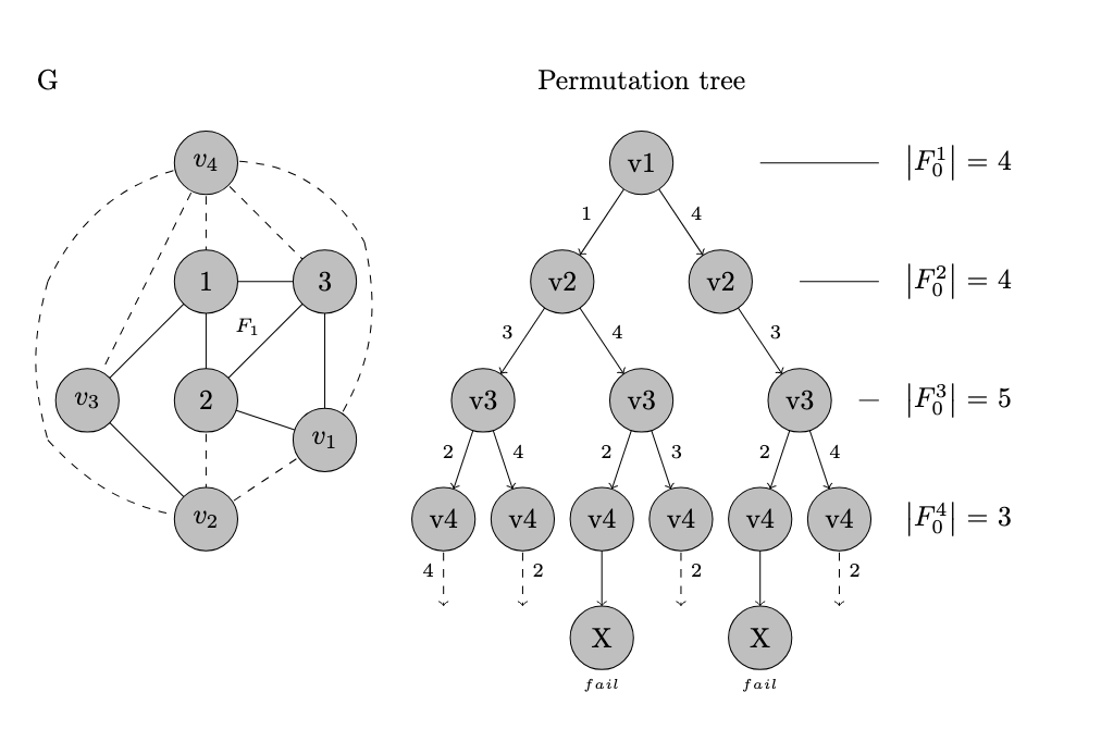
In our approach, we utilize a combinatorial tree (Pt) to systematically label the colors that can be assigned to the vertices of G. In this tree, nodes in are labelled by the vertices , which are selected during the graph reconstruction process. Meanwhile, edges in coming from record the possible colors that can be assigned to .
As the three endpoints of have assigned fixed colors, for each new vertex aggregated to , it could take a maximum of two possible colors, since . Thus, is a binary tree, whose root node is the first selected vertex .
All nodes at level of have the same label: , which corresponds to the vertex that has been added to in the iteration i. We denote as at level of . Each edge derived from is labelled with one of the colors that can be assigned to . Since , there are either one or two edges originating from , because is incident to at least two different colors in . Furthermore, if two edges come out from in , as the labels of the paths coming from are different, this establishes a system of mutually exclusive color-paths within .
A path of size of starts at the root up to level . For paths where , the last vertex is a ’dummy’ vertex (note that this dummy vertex is not illustrated in any figure of ). When the paths in are extended to one level higher (achieving level ), a new edge is inserted before the dummy vertex. Such edge connects with the dummy vertex, and the edge is labelled by the color assigned to .
Any path from establishes a 4-coloring on the vertices of . Within the paths of , there can be failure paths, which are denoted by placing the symbol X as a leaf node in the path of . Meanwhile, the parent node of X has only one unlabelled edge towards the leaf X, indicating that it is impossible to assign a color to . From a failure node X, the corresponding path is truncated and will not be expanded further.
The paths of success in are paths of length , that is, they are paths that start from , reach the vertex , and establish a single proper coloring to be assigned to each vertex on the path. The leaf node of a successful path in is labelled by E (’exit’).
Each outer face is formed by the facial cycle surrounding (the induced graph of G), regardless of the parity of this cycle, it is known that three colors are sufficient to color any simple cycle. Since the paths in represent all possible color combinations that can be assigned to , including its outer face , there will always be paths in that use only 3 colors to color . The existence of these paths will be an important property in the proof of our main theorem.
Summarizing, we utilize three support structures in the construction of a 4-coloring for a planar graph G. For an iteration , the first structure is the graph with vertices, which is induced from G. In , only the endpoints from the face have fixed colors, while the remaining vertices do not have any colors assigned. However, the colors for those vertices can be inferred from the paths in .
The second structure is the outer face corresponding to the graph . Note that since is built incrementally, its corresponding outer face depends on the last vertex added to . Lastly, the third structure is the binary tree . In , there may be failure paths; however, in the next section, we will demonstrate that there will always be non-failure paths in , regardless of the level j considered, even when reaching the maximum depth of , which is .
The following figure (Figure 6) illustrates the three structures used as support in the 4-coloring of the graph G. The order in which the vertices were selected during the reconstruction of G is indicated by the index associated with each vertex label. Notice that G is, in fact, not a maximal planar graph.
5. Proof of the Existence of a 4-Coloring for Planar Graphs
Theorem 1.
Based on the incremental and iterative construction of G by the family , for each iteration , there always exists paths in that use fewer than 4 colors for coloring the outer face of , i.e. .
Proof.
The proof is by the induction principle applied on the level of the tree: .
- 1)
-
For , the first subgraph holds that , since the outer face is a triangular face.From only two cases can be derived to form . When (illustrated in Figure 7(ii), and when illustrated in Figure 7(i). Notice that for both cases, there is a path in such that .For example, in the case . (Figure 7(ii), As one of the possible colours to be assigned to , it already appears in (in the most left path of ), does not add any new colour to the current outer face and then, .
- 2)
- By induction hypothesis, at level , there are paths in where the current outer face of has less than 4 colours, i.e. .
- 3)
-
When a new vertex is aggregated to , we form with outer face , and the combinatorial tree is extended one level more, this is from to . We analyze different cases:For the paths where , or , if assigns a color that already appears in , it will be satisfied that , and therefore, the theorem holds.Let us consider the case when , and analyze its development according to the value of .
- i)
- When , then ramifies with two possible colors, say and . If , then could have 4 colors when the color is included in . However as and , then must be in and the branch for will not increment with respect to , and therefore for this path 4 (as it was illustrated in the leftmost path of Figure 7(ii)).
- ii)
-
If . Assuming , by adding to a vertex of degree 3, the cardinality is preserved: 3 (by results from Table 1 - derived of the Euler’s equality), and therefore 4.Let us assume 3, so now we could take . This combination of parameters is analysed in the following case.
- iii)
-
To have , is only achieved by adding vertices , where , which allows increasing the cardinality of the outer face above 3, and also, it generates binary ramifications at the level , using two different colors for , let us say and .In one of the colors (either or ), we have . This is because, in all ramifications, at least one of the colors used is already present in . In fact, for all levels from k to , there are paths where for . Furthermore, according to the inductive hypothesis, there are paths at level where . Within these set of paths of , there is at least one path where the color is already included in . This is due to the exhaustiveness in the color assignment to the branches of . For these particular paths, the cardinality of does not increase for the following level; hence, we conclude that , and this confirms that the theorem holds true.Furthermore, by adding vertices with , new internal vertices are formed in , thus causing some of the colors assigned to those internal vertices to no longer appear in .
□
For example, Figure 8(i) shows that two vertices and that are added to , fulfil 2, so . The third vertex that is added to fulfils that . The tree (Figure 8(ii)) shows how paths where will always exist, regardless of the k level of the tree.
It is possible that a path would have a corresponding value of at level . Although, the same path could define at level i, a coloring for the new outer face holding . Importantly, regardless of the level i of the tree, there will be paths in where the condition is satisfied.
The previous theorem is the key in the proof of the existence of a 4-coloring for any planar graph G. By building G vertex by vertex, and forming its combinatorial tree , we acknowledge that there may be failure paths within . However, the previous theorem ensures the existence of paths satisfying the condition , regardless of the level i of the tree and the topology of the induced subgraph of G.
Corollary 1.
For any planar graph G, it always exists a 4-coloring for G.
Proof.
It is known that G can be polynomially reduced to a maximal planar graph , where all internal faces are triangular. Based on the vertex construction of and the formation of its combinatorial tree , the previous theorem guarantees the existence of paths in where , for all level i of . This ensures that whenever a new vertex is added in the vertex formation of , there is always a free color available from the set that can be assigned to .
Consequently, every vertex added to form the subgraph family, for , one of the four available colors will be assigned to each vertex. This process guarantees that a proper 4-coloring can be achieved for the graph and, consequently, for the original graph G. □
6. Conclusion
A mathematical proof of the Four Color Theorem (4CT) has eluded the efforts of scientists in the area for hundreds of years. Interestingly, the computational verification of the 4-coloring of planar graphs has been known since 1977[1,2], including refinements to the initial algorithm [9,18]. Unfortunately, the vast number and complexity of wanting to mathematically verify the thousands of configurations that can arise during the computational process have led the continued search for a formal and succinct proof of the 4CT.
This article presents a novel method that enables the enumeration of the exhaustive process involved in the 4-coloring of maximal planar graphs. Our method is based on using a combinatorial tree to enumerate all valid color combinations to be assigned to each vertex of the input graph G (except for the vertices of the innherest triangular face of G).
The breadth-first search used in constructing , while incrementally reconstructing G from its innherest triangular face, enables the analysis, construction, and encoding of all possible 4-coloring assignment functions for the vertices of G.
Our theorem confirms that in the combinatorial tree of a planar graph G, there exist paths that ensure, regardless of the size or complexity of the graph G, that each new vertex , when added to the induced subgraph of G, will always have at least one color available from the four colors that can be assigned to . Thus, confirming the existence of a 4-coloring for any planar graph. The proof of the theorem is a formal and combinatorial demonstration that is manageable by the mathematical community, due to its extent and the number of cases to be considered in its development.
Although our method guarantees that every planar graph can be colored using four colors, a future task is to propose fast algorithms based on our method, where can be developed via a depth-first search as G is built incrementally, such that upon finding the first proper 4-coloring of G, the process ends.
Funding
“This research received no external funding”
Acknowledgments
The author acknowledges and thanks the SNII-Secihti for the grant to support their work.
Conflicts of Interest
The authors declare no conflicts of interest.
Abbreviations
The following abbreviations are used in this manuscript:
| 4CC | The Four Color Conjecture |
| 4CT | Four-Color Theorem |
| 4Col | the set of all proper 4-coloring of H |
| 4c | the total number of different 4-colorings functions of H |
| Color(H) | the set of colors used in a 4-coloring of H |
| the number of different colors used in a 4-coloring of H |
References
- Appel K.; Haken W., Every planar map is four colourable, part I: discharging, Illinois Jour. Math. 1977, 21, 429-–490.
- Appel K.; Haken W.; Koch J., Every planar map is four colourable, part II: Reducibility, Illinois Jour. Math. 1977, 21, 491–567.
- Borodin O., Colorings of Plane Graphs: A Survey, Discrete Mathematics 2013.
- Bousquet N.; Deschamps Q.; De Meyer L., Pierron T., Square Coloring Planar Graphs with Automatic Discharging, SIAM Jour. on Discrete Mathematics 2024, 38:1, 504–528.
- Cortese P.; Patrignani M., Planarity Testing and Embedding, Press LLC, 2004.
- Cranston D. W.; West D. B., An introduction to the discharging method via graph coloring, Discrete Mathematics 2017, 340:4, 766–793.
- Fritsch R.; Fritsch G., The Four Color Theorem. Springer-Verlag, 1998.
- Garey, M.R.;Johnson, D.S., Computers and Intractability: A Guide to the theory of NP-Completeness, W.H. Freeman, 1979.
- Gonthier G., Formal Proof - The Four Color Theorem, Notices of the AMS 2008, 55:11.
- Harary F., Graph Theory, Addison-Wesley, Readings, Mass., 1969.
- Johnson D. S., The NP-Completeness Column: An Ongoing Guide, Jour. Of Algorithms 1985, 6, 434 - 451.
- Kempe A. B., On the Geographical Problem of the Four Colours, American Jour. of Mathematics 1879, The Johns Hopkins University Press, 2:3.
- Kuratowski K., Sur le probleme des courbes gauches en topologie, Fund. Math. 1930, 15, 271–283.
- Köbler, J.; Schöning, U.; Toran, J., The graph isomorphism problem: its structural complexity, In Graph canonization and hardness, 1993.
- László L., Graph minor theory, Bulletin of the American Mathematical Society 2006, 43:1, 75-–86.
- McKay, B.D.; Piperno, A., Practical graph isomorfism II, Jour. of symbolic computation 2014, 60, 94-112.
- Nishizeki T.; Chibam N., Planar graphs : theory and algorithms, Annals of discrete mathematics 1991, 32, Elsevier.
- Robertson N.; Sanders D.P.; Seymour P.D.; Thomas R., The four color theorem, Jour. Combin. Theory Ser. B 1997, 70, 2-–4.
- Tymoczko T., The Four-Color Problem and its Philosophical Significance, The Journal of Philosophy 1979, 76:2.
Figure 1.
Counting the number of 4-colorings on a path .
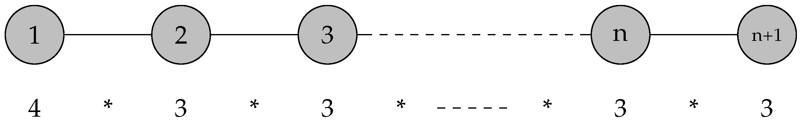
Figure 2.
Counting 4-colorings on a tree.
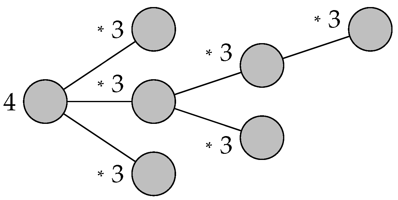
Figure 3.
counting 4-colorings on a triangle cycle.
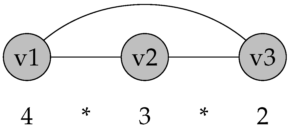
Figure 4.
Counting 4-colorings on a square cycle, considering only one of the 4 combinations for .
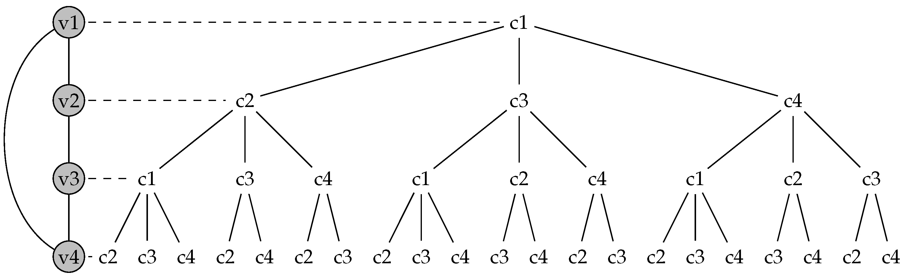
Figure 5.
The extremal planar graph minimizing the number of 4-colorings (Illustrating ).
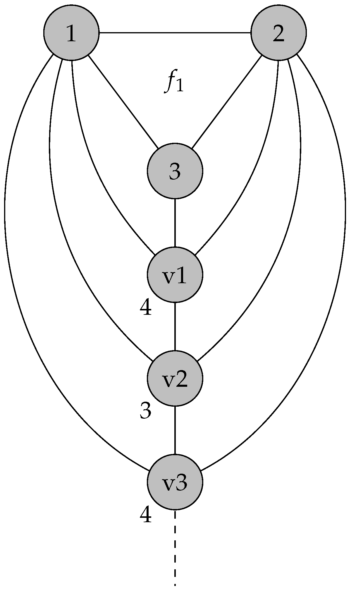
Figure 6.
Main structures used in a 4-coloring of a planar graph.
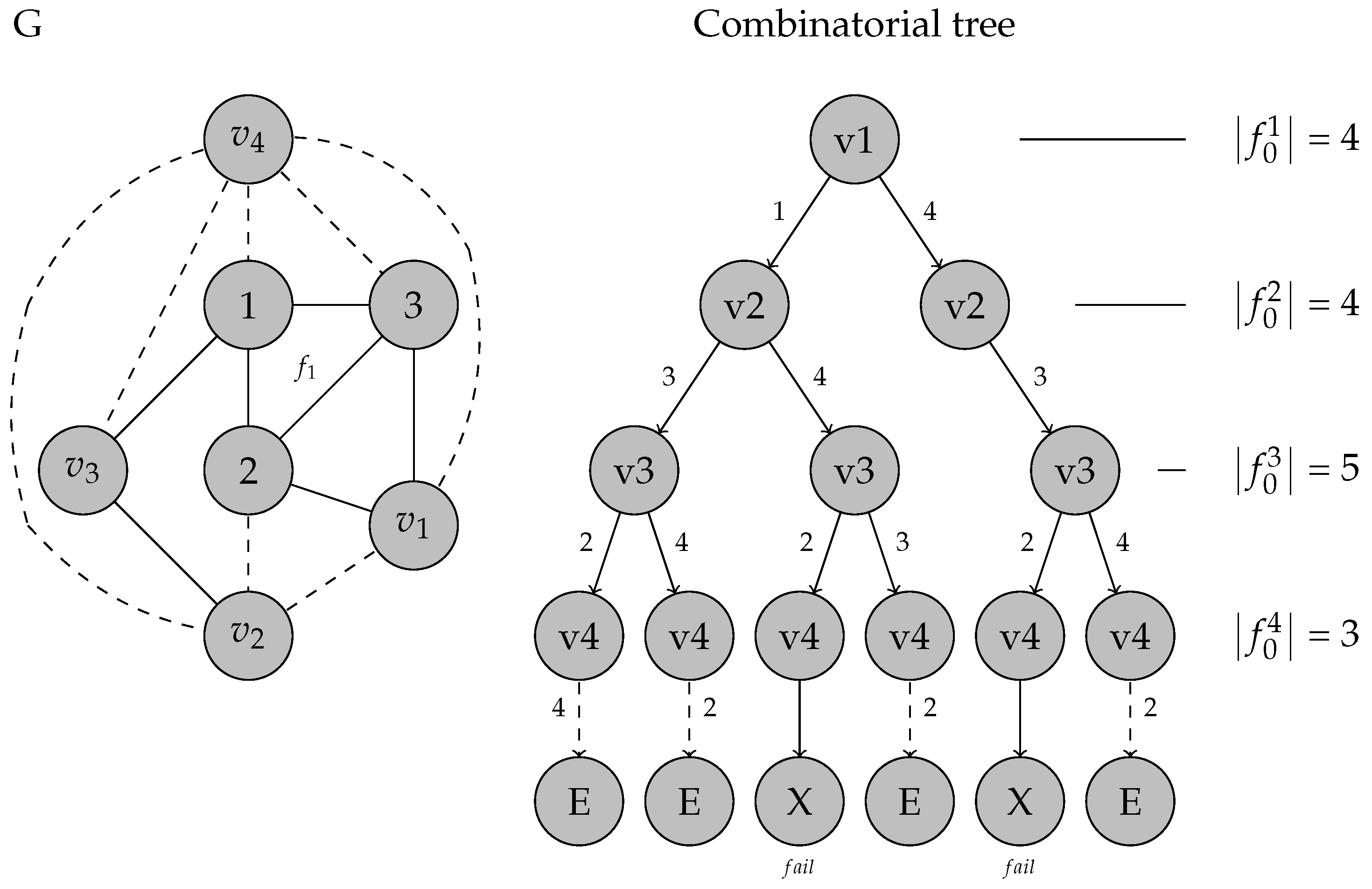
Figure 7.
i) , ii) .
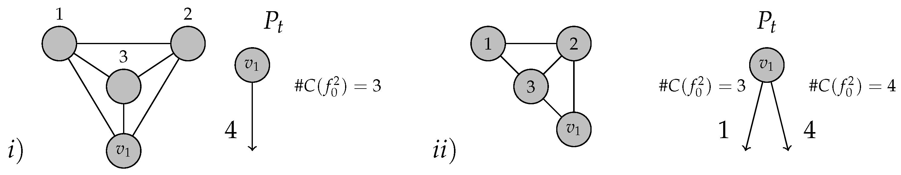
Figure 8.
i)Subgraphs with different ii) , always has paths where .
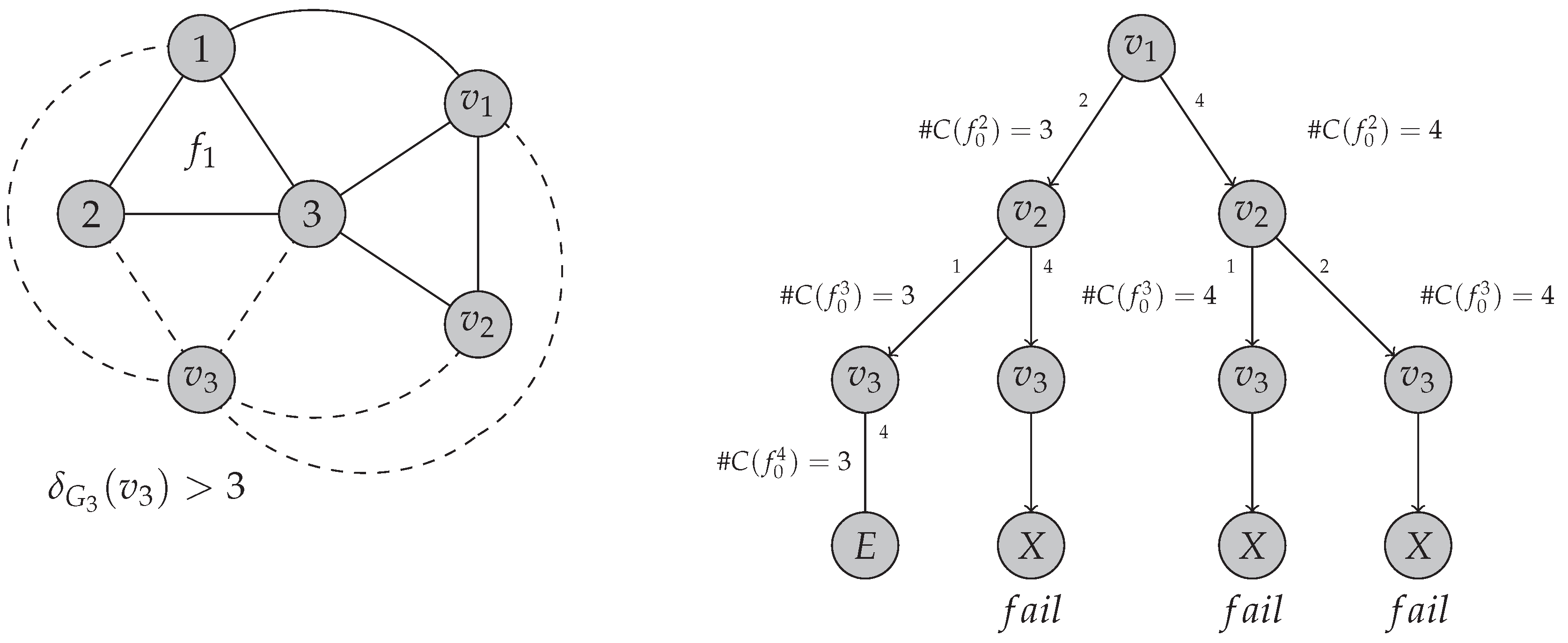

Table 1.
Growth (denoted by ) in the number of edges and faces corresponds to the increase in the number of nodes by one.
Table 1.
Growth (denoted by ) in the number of edges and faces corresponds to the increase in the number of nodes by one.
| n | m | f |
| 2 | 1 | 1 |
| 3 | 3 | 2 |
| 4 | 6 | 4 |
| 5 | 9 | 6 |
| 6 | 12 | 8 |
| 7 | 15 | 10 |
| … | … | … |
| 1 | 3 | 2 |
Disclaimer/Publisher’s Note: The statements, opinions and data contained in all publications are solely those of the individual author(s) and contributor(s) and not of MDPI and/or the editor(s). MDPI and/or the editor(s) disclaim responsibility for any injury to people or property resulting from any ideas, methods, instructions or products referred to in the content. |
© 2025 by the authors. Licensee MDPI, Basel, Switzerland. This article is an open access article distributed under the terms and conditions of the Creative Commons Attribution (CC BY) license (http://creativecommons.org/licenses/by/4.0/).
Copyright: This open access article is published under a Creative Commons CC BY 4.0 license, which permit the free download, distribution, and reuse, provided that the author and preprint are cited in any reuse.


