Submitted:
19 September 2025
Posted:
19 September 2025
You are already at the latest version
Abstract
The present paper does not intend to provide the solution of the Riemann hypothesis. Rather, we propose an alternative approach to engage with Riemann hypothesis. We assume as our working hypothesis that the Riemann hypothesis is not soluble within the current framework of the analytic number theory. Rather, we treat it as an interesting platform of empirical investigations. Four possible paths to engage Riemann hypothesis are discussed. We introduce the notion of Riemann monad Antipodal and construct a Riemann sphere model through Möbius Transformation. It follows an introduction of the Riemann sphere of two-state systems by Penrose. We regard Riemann platform as a Gauge Structure, in which the ζ function is treated as a wavefunction that satisfies gauge symmetry by performing gauge transformations. Some empirical issues are discussed. These issues are: Statistical significance; the measurement problem and the Yes/No measurement; the Dirac -function; sample space and stochastic sampling.The present paper does not intend to provide the solution of the Riemann hypothesis. Rather, we propose an alternative approach to engage with Riemann hypothesis. We assume as our working hypothesis that the Riemann hypothesis is not soluble within the current framework of the analytic number theory. Rather, we treat it as an interesting platform of empirical investigations. Four possible paths to engage Riemann hypothesis are discussed. We introduce the notion of Riemann monad Antipodal and construct a Riemann sphere model through Möbius Transformation. It follows an introduction of the Riemann sphere of two-state systems by Penrose. We regard Riemann platform as a Gauge Structure, in which the ζ function is treated as a wavefunction that satisfies gauge symmetry by performing gauge transformations. Some empirical issues are discussed. These issues are: Statistical significance; the measurement problem and the Yes/No measurement; the Dirac Delta-function; sample space and stochastic sampling.
Keywords:
Riemann hypothesis
; Riemann sphere
; monad
; antipodal
; projection
; Mobius transformation
; gauge symmetry
; wavefunction
; Penrose
; Yes/No measurement.
The Riemann hypothesis is a great entity, and the beauty of ζ function as a platform can be viewed from different angles.
1. Introduction
The Riemann Hypothesis is a long-standing open conjecture in mathematics. This mathematical conjecture was proposed by Riemann in 1859. (Mazur and Stein, 2016). The Riemann hypothesis concerns with the Riemann ζ function as follows: for any complex number ,
The Riemann analytic continuation of Riemann function is as follows,
where function, , is the analytic continuation of the factorial function on the complex plane.
Riemann Hypothesis: All the non-trivial zeroes of are on the line (called the critical line); i.e., , when .
Riemann hypothesis is important because it rather accurately predicts the distribution of prime numbers.
In 1900, at the Second World Congress of Mathematician, Hilbert proposed a list of 23 open conjectures in mathematics, of which Riemann hypothesis was listed as the number 8th. Till today, Riemann Hypothesis is regarded as the only one left being unsolved on the Hilbert list. In 2000, Clay Mathematics Institute proposed the seven greatest unsolved mathematical puzzles of our time, called the millennium problems. Of which, Riemann hypothesis is listed as the number 1. It is still standing there and people never stop investigating it.
This paper doesn’t aim at solving Riemann hypothesis, nor intends to review progresses and the current state of research along this line. There are four possible paths to engage with the Riemann hypothesis, which are briefly explained below.
Path 1. To prove or disprove Riemann hypothesis within the current framework of analytic number theory. There is a group of brave as well as perseverant mathematicians keep working this path. To keep checking Riemann hypothesis instance after instance by hoping to discover more hints of reasonable distributions. With the assistance of computer capacity, a huge amount of complex numbers has been checked, and no counter example has been found.
Path 2. To prove that Riemann hypothesis is independent of current framework of analytic number theory. This is the case like Gödel’s independent result to the first-order theory and the case like the continuum hypothesis to ZF-system in the axiomatic set theory.
Path 3. Assume Riemann hypothesis as true. Many mathematical results such as theorems and corollaries are proved or inferred. There are certain reasons to believe Riemann hypothesis holds as a huge amount of complex numbers has been checked, and no counter example has been found so far. However, such an assumption turns the study of Riemann hypothesis to be an empirical science.
Path 4. Note that no matter how many cases have been check, it is finite. Even if we keeping checking to infinity, it is only countably many. Nevertheless, the interval of analytic continuation of Riemann hypothesis is (0, 1), i.e., , and Such a domain contains uncountably many cases. Thus, if Path 3 is based on a reasonable assumption, it would be not less reasonable to assume that Riemann hypothesis is not analytically solvable; in other words, we may well assume, before Riemann hypothesis is to be proved or disproved, that the behavior of Riemann ζ as a whole is not directly observable. Hence, it can be treated as a wavefunction. This is the approach we will take to engage Riemann hypothesis. It is called a cognitive approach because its assumption is based human cognition of our current knowledge about Riemann hypothesis.
2. Riemann Monad Antipodal and Möbius Transformation
2.1. Riemann Monad
We first define two categories as below:
Definition 1. The category that contains all those complex numbers as objects that satisfy Riemann hypothesis; i.e., and . Plus, we introduce a monad A, called the Riemann monad, into the category which stands for Riemann hypothesis. Thus, there is a morphism from A to each .
The above definition is a brief version, which demands some explanation next (Hongbin Wang, personal communication, July 29, 2025). Let denote the set of complex numbers that satisfies the Riemann hypothesis; that is, and . From this set, we construct a free (strict) symmetric monoidal category , using the tensor product and a unit object I. Within , there exists an object such that , indicating that is a monoid object in . This allows us to define an endofunctor , which satisfies the monad axioms. We refer as the Riemann monad. By the similar explanation, we have,
Definition 2. The category that contains all of those complex numbers ; i.e., or . In addition, we introduce a monad , called the non-Riemann monad, into the category w. Thus, there is a morphism from each
We then introduce two complex planes as follows.
Definition 3. The complex plane is with the zero-point , where is the Riemann monad defined by Definition 1.
Definition 4. The complex plane is with the zero-point , where is the non-Riemann monad defined by Definition 2.
2.2. Möbius Transformation
We define the transformation from complex plane to as a holomorphic function : ; so that we have , which satisfies . The general transformation is as below:
where , so that the numerator is not a fixed multiple of the denominator. This is called a bilinear or Möbius transformation.
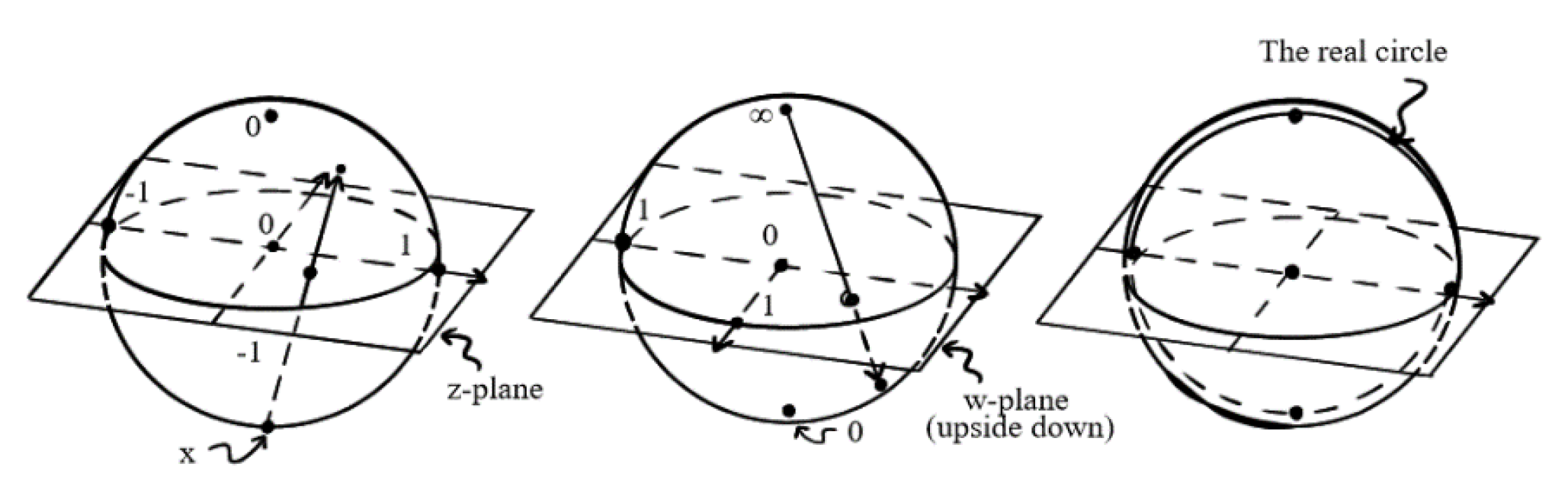
Note that the point removed from the -plane is that value which would give ‘’; correspondingly, the point removed from the w-plane is that value ( which would be achieved by ‘’. In fact, the whole transformation would make more global sense if we were to incorporate a quantity ‘’ into both the domain and target. This is one way of thinking about simplest (compact) Riemann surface of all: the Riemann sphere.
Now we assume that a theory as a piece of mind has been duplicated on machine as part of artificial intelligence based on the complex -plane and the w-plane respectively. The next step is to merge the complex planes into the so-called Riemann sphere. We regard the sphere is constructed from two ‘coordinate patches’: One of which is the -plane and the other the -plane. All but put two points of the sphere are assigned both a -coordinate and a -coordinate (related by the Möbius transformation above). But one point has only -coordinate (where and another has only w-coordinate (where We use , or both in order to define the needed conformal structure and, where we use both, we get the same conformal structure using either, because the relation between the two coordinates is holomorphic. In fact, for this, we do not need such a complicated transformation between and as the general Möbius transformation. It suffices to consider the particularly simple Möbius transformation given by
where and , would each give in the opposite patch. All this defines the Riemann sphere in a rather abstract way. See Penrose (2004, §8.3, pp.142-143) for further explanation.
2.3. Riemann Sphere
One could not help himself to make a comment: Riemann Sphere provides a beautiful picture for a path toward the unified account of mind and machine.
Figure 1.
Riemann sphere from two complex planes.
3. Riemann Sphere of Two-State Systems
The Riemann sphere above is called the conformal sphere, which puts mind and machine in one system through artificial intelligence. In this section, we introduce another kind of Riemann sphere with more structures, which is called the metric sphere. This new Riemann sphere is a two-state system. The gauge field theoretic methods can be applied to make Riemann hypothesis as a dynamic system.
Consider the function (like an electron) has an internal space. This internal space rotates. The function possesses an intrinsic property called spin which is the momentum of its internal rotation. The AI-spin has two basic eigenstates: one is Riemann monad and another is the non-Riemann monad, which are denoted as (called spin-up) and respectively. We assume the two eigenstates are orthogonal, and their linear superpositions are denoted by , which can be defined as follows,
where and are not just complex numbers but are amplitudes with certain Born probabilities. This is the reason why the corresponding Riemann sphere is a metric sphere that will be introduced shortly. The function has an internal spin of , which is similar to an electron or quark. Each state has a complex phase. The difference between two state-phases yields new a phase (by linear superposition) called the dynamic or relative phase. For more detailed discussions, please see Penrose (2004, §22.9).
The above function of the two-state (the Riemann monad vs the non-Riemann monad) can be projected to the Riemann sphere of two-states. For the Riemann sphere with a two-state system, the key concept is the notion of antipodal points, which is part of the sphere’s structure. We use the north pole to represent the spin state . In the two-state function system, the north pole represents the Riemann monad and the south pole represents the non-Riemann monad , see Figure 2 below.
Suppose that the initial state of a two-state system is represented by the point B on the Riemann sphere and we wish to perform a Yes/No measurement corresponding to some other point on the sphere, where YES would find the state at A, and No would find it at the point , antipodal to A. If we take the sphere to have radius 1/2, and projecting B orthogonally to C on the axis , we find that the probability of YES is the length , which is and the probability of NO is the length CA, which is assuming that the angle is between OB and CA with the sphere’s centre being O.
Note that the ‘Riemann sphere’ used here has more structure than that of conformal sphere and celestial sphere in that now the notion of ‘antipodal point’ is part of the sphere’s structure (in order that we can tell which states are ‘orthogonal’ in the Hilbert-space sense. The sphere is now a ‘metric sphere’ rather than a ‘conformal sphere’, so that its symmetries are given by rotations in the ordinary sense, and we lose the conformal motions that were exhibited in aberration effects on the celestial sphere.
4. Gauge Structure and Gauge Transformation
4.1. The ζ Function as a Wavefunction
From Figure 2 we can see that each superposition state B corresponds to two probabilities. This shows that superposition states are probability-wave packets. Hence, we have:
Postulate 1 (Wavefunction). We assume as our working postulate that the evolution of the ζ function is not directly observable. The ζ function can be reasonably treated as a wavefunction.
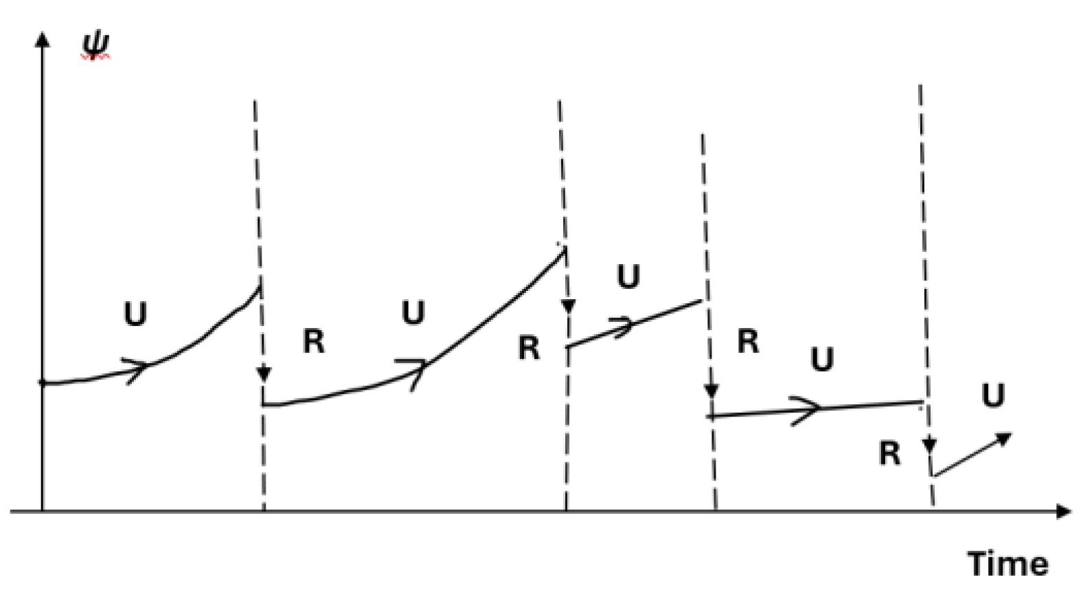
By Postulate 1, the function possesses two procedures, the ζ function the U-Procedure and the R-Procedure (U stands for unitary and R reduction). Thus, an untested complex can be seen as the superposition of Riemann monad and non-Riemann monad, which follows the U-Procedure. The Yes/No measurement of any instance will collapse the wave packet, which follows the R-procedure. This mixed process can be pictured in Figure 3 as follows (Penrose, 2004):
Definition (Prime Charge). Dynamic analysis is the sourced analysis. Keep in mind that Riemann hypothesis intends to predict the distribution of prime numbers. Thus, the driving source is named as prime charge, denoted as q.
Definition (Dynamic phase). Phase in Figure 2 is treated as the dynamic phase. At the global level, , where C is a running constant. At the local level, , which is a function.
Definition (Spin space). The function has an internal space which rotates. The spin between two eigenstates is an intrinsic property of the function.
By treating the angle (see Figure 2 above) as the dynamic phase, the gauge field theory can be applied as a modeling method. This treatment enables us to discuss about gauge symmetry of the two-state system of Riemann sphere.
The gauge structure is divided into two levels: the global and the local. At each level, it makes the distinction of the gauge potential and the field strength. The global potential is the integral format of Riemann function (i.e., its Riemann analytic continuation) as follows,
This derivative of this integral serves as the global field strength. Another way to address this issue is to treat the Riemann function as the global potential and the as the global field strength, where is the density of primes. We assume that has an internal space and it rotates. At the global level, the dynamic phase is a running constant; it may variate but does not concern the individual-state differences. At the local level, it is concerned with individual-state difference; thus, the dynamic phase is a function: .
4.2. Gauge Transformation and Symmetry
The gauge transformation is required to be conformal. This is obvious at the global level. Let the -function be a wavefunction . For the potential, we have
Consider that the dynamic phase is an any given constant, , so is also a constant. Then, to keep the forms of Lagrangian density function invariant, we can expect:
Note that is kept at the left side of as well as ; this is what makes the gauge transformation conformal. This is called the gauge transformation of the first kind, which implies the global gauge symmetry.
At the local level, the dynamic phase, is no longer a constant but becomes a phase function . The potential transforms from one state to another state is represented as:
In order to keep the gauge transformation conformal for the field strength, we need to introduce the covariate derivative and the gauge field , which are defined as below, respectively,
Then, we can see below that the gauge transformation at the local level becomes conformal,
This is called the gauge transformation of the second kind, which implies the local gauge symmetry. For those readers who are not familiar with the gauge field theoretic modeling, the derivations below would be helpful. Note that for convenience, the individual variable x is omitted from both ψ and . Then we have,
ψ = (+ig)ψ
= ψ) +ψ
= (ψ) + igψ − ig(θ)ψ
= () ψ + ψ + igψ − )ψ
= i(θ)ψ + ( + ig)ψ − i(θ)ψ
= (+ ig)ψ
= ψ.
The above derivation is given step by step for the convenience of readers who are not familiar with gauge field theory. By the above work, we established the following proposition.
Proposition 1. As a dynamic system, Riemann hypothesis satisfies the symmetry.
Note that we assumed as our hypothesis that the Riemann function is non-observable, which implies the symmetry. Consider the meaning of the well-known Nöether’s theorem, we have
Proposition 2. As a dynamic framework, Riemann hypothesis is a conservative system.
5. Issues in Empirical Science
5.1. Statistical Significance
Riemann hypothesis is a great entity and we consider the Riemann function can be viewed as an empirical science. At this point, we have
Proposition 1. The empirical evidence for Riemann hypothesis is statistically significant.
Several comments are worth mentioning about this proposition. First, Riemann considers the study of the density function of primes is more important than proving Riemann hypothesis (though it is expected). Second, the empirical evidence for Riemann hypothesis is more significant than that of any scientific hypotheses in physics. Third, though the empirical evidence may not be treated a mathematical proof or disproof of the Riemann hypothesis, it may enrich our cognition of the Riemann function. This is the reason why most mathematicians believe in that the Riemann hypothesis holds. Many mathematical results are driven by such a belief. Finally, the empirical method used in investigation of the Riemann hypothesis may provide new ideas as well as new methods for a possible pure mathematical solution of the Riemann hypothesis. Thus, looking into the mathematical issues of empirical methods applied in studying Riemann hypothesis and function can be insightful.
5.2. The Measurement Problem
The measurement problem, also called the measurement paradox by Penrose (2004), is a well-documented issue in quantum physics. It has caused some longstanding controversies in quantum mechanics and a great deal of debates. The present paper aims to provide an alternative solution for the measurement problem. In order to tackle this paradox, we have to face a challenging inquiry: Shall we take the observation as part of the theory, or not. For this, we take the former approach.
The measurement paradox reflects a very deep issue about how we understand quantum physics. On one hand, by Dirac, the greater the degree of disturbance in our observation, the smaller the world we can observe. Quantum theory is about small world. Here, the disturbance in our observation should include the limitation of our experimental methods. I would add some words here that the smaller the world, the more important and more sensitive the observation. On the other hand, at the very bottom line, quantum physics is an empirical science, so it cannot stand without observations. As Penrose points out (2004), “Some people might take refuge in the viewpoint that quantum states are ‘not real things’ being ‘not measurable’, or something”.
Nevertheless, Penrose believes that there are powerful reasons for expecting change. Such a change, to Penrose’s view, represents a major revolution and it cannot be achieved by tinkering quantum mechanics. Yet, the necessary changes must themselves be thoroughly respectful of the central principles that lie at the heart of present-day physics, which is the same as the basic aim of this paper. Let us review a few key concepts concerning the measurement paradox.
5.3. Observable Q and Projector E
The measurement paradox can be simply characterized as U-procedure versus R-procedure. Here U stands for unitary, and R stands for reduction. On one hand, the U procedures work so supremely well for simple enough systems, whereas on the other, we have to give up on U and abruptly, yet stealthily, interpose the R process from time to time. The two quantum processes, U and R, are conflicts. On the one hand, U-procedure is the deterministic process of unitary evolution which can be described by Schrödinger’s Equation which controls the clear-cut temporal evolution of a definite mathematical quantity, namely the state vector The wavefunction in the U process is single-valued, continuous, differentiable, and square-integrable. On the other hand, R-Procedure is the quantum state reduction which takes place when a ‘measurement’ is performed. The R process is a discontinuous random jumping of this same , where only the probabilities of the different outcomes are determined.
Observable operator Q is responsible to transfer from U-procedure to R-procedure. Q has two eigenstates, say, one is YES and the other is NO. How Q works is a mystery. Penrose (2004) reviewed and discussed six approaches toward this problem.
The projector E was originally introduced by von Neuman (1955). Penrose (2004) provides a thorough characterization of E. Consider an any given wavefunction , ranges over all space points of X. For any given space point Q, where stands for a testing point. Then, E projects to be Yes or No. We call it the E operation, which stands for the any given Y/N observations.
5.4. The Yes/No Measurement
The Yes/No type measurement originally proposed by von Neuman (1955) and outlined in detail by Penrose (2004). Both authors stated that all the quantum theoretic experiments are Y/N type measurements. In Penrose’s book, §22.5 is titled: Yes/No measurement. It is the view of von Neuman and Penrose that all the quantum measurements are the Yes/No type measurements. Once observation operator Q turns a quantum process into the R-procedure, then E projects the quantum state to Yes or else No. In other words, the projector E has exactly two eigenstates.
To solve the measurement paradox, the existentiality is not enough. It needs to further formulate a constructive proof. The Yes/No type measurement enables us to recapture paradox of U-procedure vs. R-procedure. From mathematical perspectives, it is a single-valued vs. two-valued problem. During the U-procedure, the wavefunction is single valued. While during the R-procedure, any measurement of the wavefunction becomes two-valued.
5.5. The Dirac -Function
In empirical sciences, particularly for the evaluation tasks, the Dirac Delta Function is the first step of mathematical characterization, which we provide one more time as follows
where the formula (2) is the analytic continuation of the formula (1). In measurement theory, in (2) is called a testing function, and in (1) is the supporting point of (Griffel, 1981/2002). In our context, we can immediately recognize that can stand for the Riemann-monad A and x ranges over all possible states (i.e., complex numbers ). Thus, the formula (1) can be rewritten as follows:
where A is the Riemann monad and the arrow represents the morphism from A to the non-trivial zeroes of Riemann function. Interestingly, the formula (2) makes such a commitment that no matter a state is a nontrivial zero of the Riemann function (i.e., marked as yes or no), the integral as the potential is a constant. In other words, at the global level, the Riemann function rotates from one state to another with constant dynamic phase. It also shows that the Riemann hypothesis is a conservative system.
Now we look at an important property of the -function. For an any given one-dimensional wavefunction , assume () is a R-interval, we have
This is what is called the selectiveness property of the Dirac -function. Let be the Riemann function, we have
where is the Riemann monad; this is exactly predicted by the Riemann hypothesis.
5.6. Other Empirical Issues
To treat Riemann function as a wavefunction, it will meet a number of empirical issues which we briefly explain below (Yang, Y. 2024).
Issue 1 (probability wavefunction). we would assume it is not directly observable so that it should be treated as the U-process (U stands for unitary) by Penrose (2004). Accordingly, the testing observation is the R-process (R stands for reduction).
Issue 2 (observation operator). Let us consider an any given wavefunction (x), where x ranges over all of the space points. We assume that (x) is one-dimensional without loss of generality for multi-dimensions. Thus, the corresponding Hilbert space we are currently discussing is one-dimensional, denoted by H. Hence, we may treat all the vectors in H as space points also without loss of generality. Now, we introduce an observation operator Q. For any given a, , . We call that is the observational conjugate of . Accordingly, we define | ranges over all possible observational . Call the observational dual space of .
Consider the power set of , . Now, we start to select the elements from . Notice that this selection process is countable, but the cardinal number of is an uncountable infinity. We may reasonably assume this selection process is stochastic.
We introduce a new variable , . Of course, we also have , so we can introduce another variable , where the superscript j indicates the jth element stochastically selected from , the subscript i indicates that x ranges over only those space points within . It is easy to see that connects and . Accordingly, we introduce a new operator , called the sample generator. , . Call the testing adjoint of .
Issue 3. Stochastic sampling. For any given once a is stochastically selected, its adjoint becomes a testing sample. 2. For any , if it has not been selected, then its adjoint is not a testable sample yet. here the definition of stochastic sampling process is necessary to bridge any from sampling perspectives.
Issue 4 (R-procedure). Let stand for an any given sample , denote a YES/No type experiment, and q be a Yes/No type stimuli that can use to test . By Dirac bra-ket formalism, we can write this structure as . When gives the stimulus q to , each operational conjugate in returns a Yes/No type response. Thus, is a function of . This is called the R-procedure of the wavefunction. Note, this idea is from Feynman (1965), who calls the final state and the initial state of a quantum theoretic experiment.
Issue 5 (Sample space). The sample space for the Yes/No type measurement is two-valued, i.e., This means the E-projector has two and only two eigenstates, of which the eigenvalues are Yes and No. Consider projector E, for each proper sample of Yes/No type measurement, produces a pair of the yes-number c and the no-number d, which in turn produces a sample phase with respect to the exponential form of . All the possible sample phases form an group, write it G. From Definitions 1 to 4, it is easy to see that G is originally generated from the wavefunction , so we write G as .
Because symmetry, the stochastic sampling here satisfies the required conservativeness. It is worth mentioning that, in addition to the well-documented dynamic phase and Berry phase in the literature of dynamic analysis, the sample phase introduced here is the third kind of phase. This is one significant character of the R-procedure. For the U-procedure, we have the dynamic phase potential group, write it as .
Issue 6 (linearization and sample Born probability). The linearization operator L is defined by ). For any given testing sample , which produces a yes-number and a no-number . the sample Born probability is defined by
Born probability is a kind of explanation, which serves as a semantics for the evolution of wavefunction. As Penrose pointes out (2004), the U-procedure and R-procedure must share the same semantics, i.e., the squared magnitude of two eigenvalues. It is easy to see that the Born probability here obeys Born rule. Let be a testing sample. eigenstates, Yes or else No. Assume the eigenvalue for Yes is c and the eigenvalue for No is d. Then, by Definition 8, we have ). Hence, we have
6. Concluding Remarks
Remark 1. The present paper did not provide a solution of Riemann hypothesis. Rather, by assuming the Riemann hypothesis is unsolvable within the current framework of Riemann analytic continuation (Yang, 2025), we outlined an alternative approach to engage the Riemann hypothesis from perspectives of the empirical science.
Remark 2. We demonstrated that the Riemann hypothesis can be modeled by a Riemann sphere of two-state system. This is done in two steps. First, it introduces the Riemann monad and the non-Riemann monad as a pair of antipodal. Second, the corresponding Riemann sphere is formed by the Möbius transformation.
Remark 3. The Riemann ζ function can be treated as a wavefunction with a dynamic phase. By performing gauge transformations, the rotation of the dynamic phase satisfies certain gauge symmetry. The local gauge symmetry is achieved by introducing the notions such as the prime charge, the covariate derivative, and gauge field.
Remark 4. The evolution of the Riemann ζ function experiences two kinds of processes: the unitary procedure and the reduction procedure. The R-procedure performs the Yes/No measurement.
Remark 5. As the last part of the paper, a number of empirical issues are addressed. These issues are concerned with the measurement problem, stochastic sampling, amplitude semantics and Born probability.
Acknowledgments
The author thanks his students who did the first-round proofreading. In particular, I want to thank Aliya Yang and Xin Fu for their help in preparation of the figures.
References
- Griffel, D. H. (1981/2002). Applied Functional Analysis. Dover Publications, Inc. Mineola, New York.
- Mazur, B. and Stein W. (2016). Prime Numbers and the Riemann Hypothesis. Cambridge University Press.
- Penrose, R. (2004). The Road to Reality – A Complete Guide to the Laws of the Universe. Random House, New York.
- Von Neumann, J. (1955/2018). Mathematical Foundations of Quantum Mechanics. Princeton University Press.
- Yang, Y. (2025). An Independence Result on Riemann Hypothesis: A Gödel Metalogic Approach. [CrossRef]
- Yang, Y. (2024). The Revised Schrödinger Equation as a Solution of Measurement Paradox: A Unified Model of the U-procedure and R-procedure. [CrossRef]
Figure 2.
Riemann sphere of two-state system.
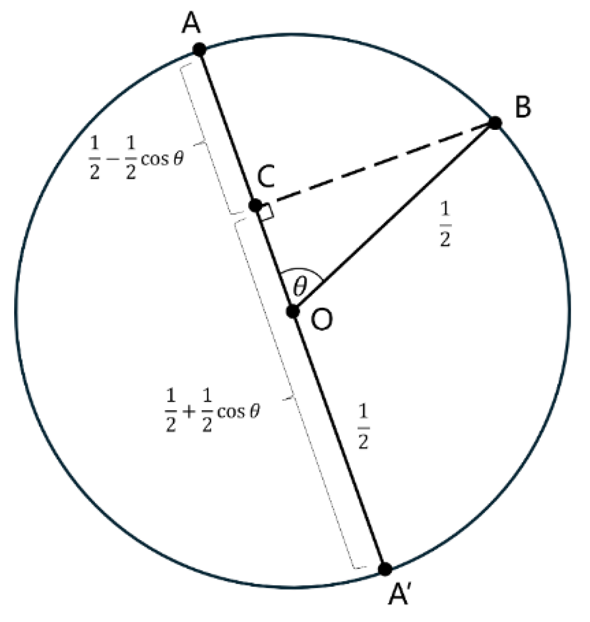
Figure 3.
The U-Procedure and the R-Procedures of the wavefunction.
Disclaimer/Publisher’s Note: The statements, opinions and data contained in all publications are solely those of the individual author(s) and contributor(s) and not of MDPI and/or the editor(s). MDPI and/or the editor(s) disclaim responsibility for any injury to people or property resulting from any ideas, methods, instructions or products referred to in the content. |
© 2025 by the author. Licensee MDPI, Basel, Switzerland. This article is an open access article distributed under the terms and conditions of the Creative Commons Attribution (CC BY) license (http://creativecommons.org/licenses/by/4.0/).
Copyright: This open access article is published under a Creative Commons CC BY 4.0 license, which permit the free download, distribution, and reuse, provided that the author and preprint are cited in any reuse.


