Submitted:
17 September 2025
Posted:
22 September 2025
You are already at the latest version
Abstract
Monitoring bottom-hole pressure (BHP) is critical for reservoir management and flow assurance, especially in offshore fields where challenging conditions and production losses are more impactful. However, reliability issues and high installation costs of Permanent Downhole Gauges (PDGs) often limit access to this vital data. Soft sensors offer a cost-effective and reliable alternative, serving as backups or replacements for physical sensors. This study proposes a novel data-driven methodology for estimating flowing BHP using wellhead and topside measurements from plant monitoring systems. The framework employs ensemble methods combined with clustering techniques to partition datasets, enabling tailored supervised training for diverse production conditions. Aggregating results from sub-models enhances performance, even with simpler machine learning algorithms. We evaluated Linear Regression, Neural Networks, and Gradient Boosting (XGBoost and LightGBM) as base models. A case study of a Brazilian Pre-Salt offshore oilfield, using data from 60 wells across nine platforms, demonstrated the methodology’s effectiveness. Error metrics remained consistently below 2% across varying production conditions and reservoir lifecycle stages, confirming its reliability. This solution provides a practical, economical alternative for studies and monitoring in wells lacking PDG data, improving operational efficiency and supporting reservoir management decisions.
Keywords:
reservoir engineering
; soft sensors
; regression analysis
; neural networks
; gradient boosting
1. Introduction
A key challenge in petroleum engineering is monitoring reservoir and production parameters throughout the lifecycle of wells and reservoirs. Tracking pressure, temperature, and production rates over time is essential for detecting anomalies, identifying issues like scaling or reservoir damage, understanding reservoir configuration, forecasting performance, and optimizing recovery. Reliable, continuous data acquisition is crucial for reservoir engineering, well testing, flow assurance, and operations management.
In modern offshore production systems, these measurements are collected at various nodes of the production and flow system, as described below (and illustrated by Apio et al. [1]):
- Topside: Measurements of oil, water, and gas production rates (, , and ), along with pressures and temperatures upstream and downstream of the choke valve.
- Wellhead: Measurements of pressure and temperature via temperature and pressure transducers (TPTs).
- Bottom-hole: Measurements of pressure and temperature via permanent downhole gauges (PDGs).
Among these, PDGs are arguably the most important, as they are located near the reservoir and provide essential data on its behavior, notably the Bottom-Hole Pressure (BHP) [1,2]. However, they are also the most prone to failure [3] due to harsh operating conditions (high pressures and high temperatures) [4] and the long distances that signals must travel to reach the monitoring stations at the platforms. Moreover, PDGs are the most challenging to replace, as they are positioned at the bottom of wells, and that would require complex and costly workover operations, that are rarely economically viable [5].
In oilfields with lower productivities and revenues, even the initial installation costs of PDGs in all wells may be prohibitive. In cases where PDG signal loss occurs or new installations are not feasible, the use of Soft Sensors becomes an essential alternative.
Soft sensors (or software-based sensors) refer to a suite of methods and tools designed to replace/backup physical sensors (the “hard” sensors) or enable the monitoring of variables that are difficult or impossible to measure directly, due to challenges as hostile and unreachable environments, disturbances to the process, measurement delays, or high costs [6]. They can be used to estimate the values of real physical quantities, or other virtual variables, as quality metrics for industrial processes [7], and can be used in real-time applications [8] including digital twins.
The development of soft sensors can be based on methods as mathematical relationships, statistics, and data-driven machine learning (ML), among others, as well as their combination with analytical hardware data [6,7].
In the field of oil and gas exploration and production, the literature primarily features studies utilizing soft sensors as virtual meters for flow variables and downhole quantities. For the first group, a common problem addressed in the literature regarding petroleum production systems is the allocation of individual well production rates. This is relevant because the production from a group of wells, e.g., all those on a platform, is typically combined in a single separator vessel, and daily flow measurements for accounting and regulatory purposes are performed for the total output [9]. Individual rates must then be calculated/estimated to support other activities—we will later discuss how this impacts our work. This can be done simply by distributing based on the most recent individual measurements, but soft sensors can improve these estimates by providing values per fluid and per well based on other continuously measured variables, such as sensor data.
The use of data-driven methods for this purpose is studied by Paulo et al., who used system identification techniques to obtain a black box model to predict liquid flow rates from available field measures as pressures and temperatures [2]. Song et al. developed a virtual flow meter for an offshore oil platform, and compared the results of models based on Multi-Layer Perceptron (MLP) neural network, random forests, and Long Short-Term Memory (LSTM) networks. They evaluated the data volume required for reasonable results and the positive impact of using transfer learning to reduce that volume [10].
The work of Góes et al. proposed mathematical models to estimate the rates using real-time data from the plant monitoring system and offline data as fluids properties [11]. A combination of physics-based and data-driven methods is proposed by Ishak et al., using ensemble learning for a virtual multiphase flow meter [12]. The recent work of Alves et al. uses Neural Networks as proxy models for a physics-based simulator to perform data reconciliation online in real time for monitoring purposes [9], while Rabello et al. deploy parallel computing techniques to improve the performance of data reconciliation for the same problem [13].
A different application in flow, the sequential transport of different fluids through a pipeline, is studied by Yuan et al., who use a knowledge-informed Bayesian-Gaussian mixture regression model to track the fluid interface along the way, serving as an example of a soft sensor for a virtual variable [14].
A more comprehensive review of works on virtual flow meters is brought by Bikmukhametov and Jäschke [15].
Regarding bottom-hole variables, Semwogerere et al. developed and deployed a soft sensor fusion model to monitor temperatures in annuli that cannot be measured by traditional sensors [16]. However, the applications of soft sensors for downhole variables are usually focused on estimating pressures. One relevant application is monitoring BHP in drilling operations, as we can see in the works of Ashena and Moghadasi, Zhang et al., and Zhu et al., all using machine learning methods having as inputs some easily measurable drilling parameters [17,18,19].
For the production phase, we have examples of BHP estimation for static, transient, or steady-state. Prediction of pressure evolution during extended shut-ins is studied by He et al., comparing the results of a machine learning model and a physics-based data-driven one [3]. Apio et al. focus on BHP estimation under slugging conditions, comparing the results of a black box neural network (NN) model and a grey box one (Kalman Filter) [1].
More aligned to our own work, other authors approach flowing BHP under steady-state using different methods. Zalavadia et al. developed a hybrid method, using physics-based and machine learning models, where for each sample the best correlation is selected and subsequently the estimation is improved using the ML; they use as inputs a mix of static (e.g. Pressure-Volume-Temperature properties) and dynamic data (as rates and sensors) [20]. Aggrey and Davies use NN as a virtual PDG sensor, having as inputs pressure and temperature data from other sensors and the positions of the intelligent completion for an offshore well [5].
Eltahan et al. proposes a ML approach to improve BHP calculations by deriving correction factors for empirical correlations. They train separate ensembles of linear regression, support vector regression (SVR), and random forest models, using the full training dataset for each method. Predictions from multiple models within each algorithm are averaged to produce final results. Testing on 11 multi-fractured horizontal wells validates the framework’s effectiveness in refining BHP estimation [21].
Ignatov et al. employed tree-based ensemble methods–Random Forest and XGBoost–to estimate BHP using dynamic production parameters and basic well geometry features. The models were validated using a dataset generated from multiphase flow simulations in wellbores, demonstrating the validity of the framework for pressure prediction in complex flow regimes [22].
Campos et al. estimate flowing BHP using bottom-hole temperature, wellhead pressure, flow rates, depth, and tubing internal diameter for radial-based functions (RBF) neural networks, with weights optimized via particle swarm optimization (PSO) [23]. The work of Tariq et al. deploys a PSO-adjusted neural network for this estimate, highlighting the capability of use in real-time applications [24]. Also using a similar set of input variables, Nwanwe and Duru gave preference to a white-box approach, using an adaptive neuro-fuzzy model, which performed significantly better than empirical correlations and mechanistic models [25].
The work of Terminiello et al. focus on multi-fractured onshore wells, highlighting that in such plays is not usual to install PDGs in wells after the initial phase of development. Their method is mainly based on wellhead pressure, but adding information on well geometry, production, and fluid properties, feeding Extreme Gradient Boosting (XGBoost) and Categorical Boosting (CatBoost) estimators, whose outputs are combined (mean value) for the final results [26].
Rathnayake et al. compare the results of the XGBoost and a mixed-effects linear regression for pressure estimation in coal seam gas (CSG) wells, using production rates, pressures from other sensors, and pump parameters [27].
Zheng et al. approached the problem using knowledge-guided machine learning, by integrating physics-based loss functions to the models. That loss is calculated from two-phase flow pressure drop equations and its use improved the accuracy of both NN and XGBoost models [4].
In their work on BHP estimation, Agwu et al. applied multivariate adaptive regression splines, demonstrating its effectiveness through a combination of high predictive accuracy and interpretability. They underscored the model’s suitability for real-time applications, particularly in operational settings where transparency and physical consistency are critical. Additionally, they contributed an extensive literature review that traces the chronology of data-driven BHP estimation techniques [28].
What most of these studies have in common is the attempt to leverage machine learning and hybrid models to achieve more reliable results than those obtained through traditional methods, such as empirical correlations, while being more practical to handle compared to numerical simulations.
Our previous work [29] addressed this problem with a narrower scope, limited to a single platform. Leveraging a deep learning technique, the LSTM networks, yielded slightly better results than those obtained using neural networks and linear regression with ridge regularization.
In this study, we take a step further by expanding the scope to a complete giant oilfield composed by two isolated reservoirs, utilizing data from nine platforms and 60 production wells. This includes a wide range of production conditions, covering significant variations in flow rates, water cuts, and gas-oil ratios, as well as the use of artificial lift via continuous gas lift in some wells. A proposed strategy to enhance estimation within this complex domain involves partitioning the data space using clustering techniques and training ensembles of predictors for the resulting subsets.
This approach has been explored in some industrial applications. Kim et al. developed a clustering-based hybrid soft sensor to improve melt index monitoring in polypropylene production, dividing the operational conditions into four clusters using a Critical to Quality-based method, and developing ML models for each of those. Applied in the industry as real-time monitoring, the soft sensor improved the process by reducing off-specification products [30].
Yang et al., address the challenge of developing soft sensors for nonlinear and multimodal industrial processes, where global modeling struggles to represent complex and unbalanced data distributions. They propose a Quality-Relevant Feature Clustering, which through balanced grouping and the use of a regulation variable optimizes feature representation and improves the ML estimation of oxygen concentration in an ammonia synthesis plant [31].
To predict carbon content and temperature in steelmaking processes, Gu et al. developed a method combining clustering and ensemble learning. They employ a graph convolutional network-based supervised clustering to group data into subsets, guided by process labels. Local models trained on these clusters are integrated through grey relational analysis, weighting predictions based on similarity to cluster patterns. This strategy showed effective handling volatile industrial data and improving endpoint control [32].
The use of clustering strategies for domain partitioning, however, remains a novel contribution within the context of soft sensor applications for oil wells, and this work aims to address that gap.
1.1. Traditional Approaches to Flowing BHP Estimation
Estimating pressures along the path from the wellbore to the platform is a highly complex task due to the characteristics of multiphase flow. Along this path, there are some predominantly vertical sections, such as in the tubing and riser, some predominantly horizontal sections in the flowlines, and even downward-sloping sections in connections with lazy-wave configurations. Additionally, the properties of the transported fluids change along this path, as gas is released from the oil as the pressure decreases below the bubble point. The combination of these factors results in multiple possible flow regimes in the pipelines (e.g., annular, bubbly, slug), directly influencing the pressure gradients—gravitational, accelerational, and frictional. The main challenge, therefore, lies in understanding the phase distribution and interface geometries, a problem that often lacks an analytical solution and cannot always be solved, even using advanced simulations such as Computational Fluid Dynamics (CFD) [33].
Traditionally, multiphase flow calculations are performed using empirical correlations, such as the classical models of Beggs and Brill [34], Duns and Ros [35], and Hagedorn and Brown [36]. Even decades after their publication, these correlations remain widely used in the industry, serving as the foundation for several simulation software applications.
However, these correlations are typically defined for specific conditions and face limitations when applied across a broad range of production parameters [20]. Changes in flow regimes and the concept drift associated with the evolution of well and field production lead to a loss of accuracy and the need for correlation adjustments. Some simplifications are also common in this approach, such as neglecting phase slippage or assuming a homogeneous fluid [37].
Mechanistic approaches, while grounded in flow physics, are often even more restrictive in their applicability, as they generally assume a single flow regime and adopt simplifications of the governing phenomena [20].
These application range limitations also extend to simulation software. While these tools are capable of providing more detailed pressure and temperature gradient estimations, conducting sensitivity analyses, accounting for gas lift operations, and calculating flow rates based on boundary pressure conditions, they still rely on models that require updated parameters reflecting the well conditions, such as Inflow Performance Relationships (IPR). This is particularly relevant for the field where we aim to apply our framework, where well models are typically updated after production tests, when a well stream is individually routed to a separator to accurately measure its production rates and pressures [9,13,37].
Data-driven methods can fill some gaps among the previous methods, considering that they allow us to develop soft sensors even if there’s no explicit knowledge about the relationships among variables [8], a characteristic that can be useful for obtaining new insights and exploring new applications. Our work does not aim to replace existing tools but rather to serve as an additional resource for simpler and more general use in situations where traditional tools have limitations.
1.2. Objectives and Motivation
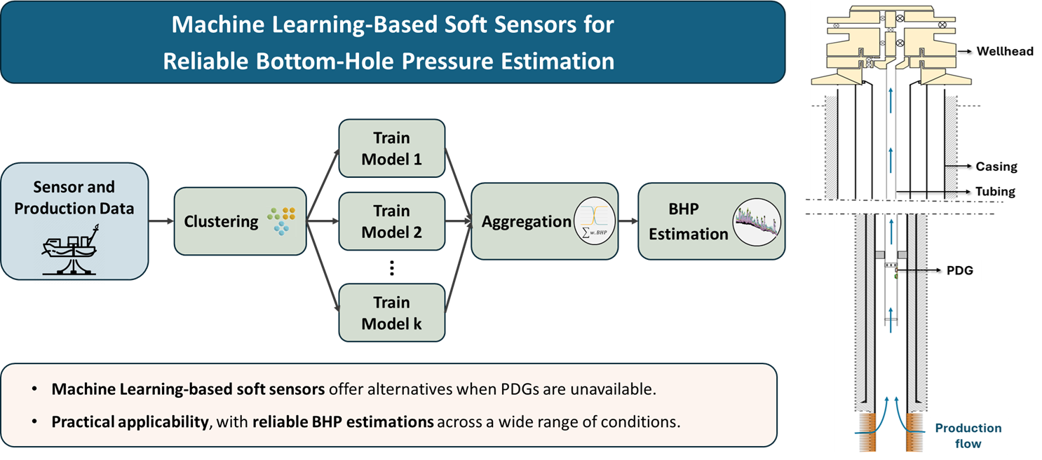
This study aims to estimate the flowing bottom-hole pressure of oil wells in regular operation by employing a novel data-driven methodology based on ensemble machine learning techniques. Our primary goal is to create a soft sensor capable of providing reliable instantaneous BHP estimates, suitable for real-time reservoir and well monitoring. The framework is particularly valuable in situations where permanent downhole gauge data is unavailable. By using surface measurements and wellhead gauge data, this methodology eliminates the need for analytical models, empirical formulas, or detailed fluid property information.
An important requirement is obtaining a comprehensive method applicable to fields with varying production conditions. This includes newly drilled wells with high production rates, original gas-oil ratio (GOR), and near-zero water cut, as well as mature wells that have been producing for over a decade. These older wells may be located in more depleted areas of the field, resulting in lower flowing pressures and production rates, and may be influenced by injection processes, leading to significantly higher GOR and water cut. Such diverse conditions can lead to varying relationships between the input variables and the target variable in our estimation problem. Addressing this variability is crucial to ensuring the robustness and applicability of the proposed methodology across a wide range of field scenarios. As we previously mentioned, the alternative we propose involves “partitioning” the problem, making it more manageable for simple machine learning methods that will be trained on subsets and have their results aggregated a posteriori (according to the methodology detailed later in a dedicated section).
We compare multiple machine learning models for the task: Ridge Regression, Gradient Boosting (XGBoost and LightGBM), and Multi-Layer Perceptron Neural Networks. Those models were chosen to allow an evaluation of diverse characteristics and levels of complexity, enabling us to compare performance on the task and assess how they can benefit from the ensemble framework. We prioritized high adaptability to the problem and low computational cost, with interpretability considered an additional advantage. From our proof of concept [29], we observed that the performance differences between simple and complex models were not particularly significant in the context of our problem and dataset. This insight motivated us to experiment with the ensemble approach using regularized linear regression and non-deep neural networks with the classic multilayer perceptron architecture. We also include methods that are intrinsically composed of ensembles, particularly tree-based. The characteristics of our problem, based on a comprehensive dataset with relatively low variability and no relevant tendency to overfit, led us to prioritize boosting strategies (over bagging and Random Forests strategies) [38]. Consequently, we selected XGBoost and LightGBM because of their demonstrated efficiency across a wide range of problems in recent literature and data science competitions, balancing predictive accuracy with computational efficiency [38].
To assess the performance of the proposed methodology, we applied it to datasets from a Brazilian Pre-Salt offshore oilfield, where all wells were originally equipped with Permanent Downhole Gauges (PDGs). Over time, however, a significant number of these gauges became inoperative. As a key motivation for this work, our statistical survey of sensor availability—conducted across nine platforms operating in the selected oilfield—revealed that downhole gauge failures occur up to three times more frequently than those at the wellhead. Moreover, the replacement of PDGs is considerably more expensive and logistically complex. Based on our survey findings, the proposed virtual sensing methodology is immediately applicable to at least 15 wells in the field that currently lack reliable PDG data. We emphasize the scalability of the approach, which can be extended to other platforms or oilfields where PDG data is unavailable or where the installation of such sensors is not economically or technically viable, provided that the necessary input variables are available and a representative dataset exists for model training
Key contributions of this work include:
- Utilizing clustering techniques to improve training efficiency for varying production conditions;
- Demonstrating adaptability across different reservoir and flow scenarios, validated for wells at various production stages;
- Offering a practical monitoring solution for wells lacking PDG data.
We believe that these characteristics distinguish our work from existing studies in the literature, representing an advancement in this research domain.
2. Materials and Methods
In this section, we provide a detailed account of the implementation of our methodology, outlining the theoretical foundations and their application to our specific case. The sequence of the process is illustrated in the flowchart in Figure 1, and the steps are detailed in the following subsections.
2.1. Data Acquisition
This study focuses on an offshore oilfield located in the Brazilian pre-salt basin with two different accumulations, where nine production platforms operate, each covering distinct areas of the field and at varying stages of their life cycle. Within this context, data was collected from a selected set of 60 production wells. We utilized a Python Application Programming Interface (API) to retrieve data from the Plant Information (PI) system, granting access to the historical sensor data collected in real time from wells and platforms. The data used in this study includes over 100,000 instances, covering a diverse range of production conditions and operating regimes, what makes it one of the most comprehensive in scope in the literature, as we can see comparing to the compilation presented by Agwu et al. [28].
Data preparation began with gathering all the identification tags for the required sensors, cross-referencing them with the schematics of well completions. Some wells are equipped with multiple Permanent Downhole Gauges (PDGs), for instance, one measuring pressure and temperature inside the tubing and another in the annulus, or at different depths in the case of selective completions for multiple intervals. In such scenarios, we prioritized the tubing PDG located at the uppermost position. Figure 2 illustrates some possible completion configurations, highlighting the positions of the PDGs.
It is important to highlight that bottom-hole temperature (BHT) data is available; however, since our objective is to estimate bottom-hole pressure (BHP) in the absence of a PDG signal, we opted not to utilize data from another variable measured at the bottom hole. This decision stems from the fact that the most common failure mode involves the simultaneous loss of both temperature and pressure PDG signals.
Additionally, we retrieved wellhead pressures (WHP) and wellhead temperatures (WHT), measured by the Temperature and Pressure Transducers (TPT), as well as the surface measures at the inlet of the choke valves, consisting in pressures (Choke P), temperatures (Choke T), and valve apertures (Choke Ap).
The dataset utilized in this study is characterized by significant variability in reservoir and fluid conditions, both spatially and temporally. This variability is driven by several interrelated factors: (1) compositional differences in the original reservoir fluids due to the extensive size of the reservoir; (2) the evolution of drainage patterns in distinct areas of the reservoir over time; (3) geological heterogeneities within the rock formations; and (4) the application of varied recovery strategies, such as Water Alternating Gas (WAG) injection. Furthermore, disparities in perforation intervals, well architecture, and flowline configurations introduce additional complexity to the flow conditions. These combined factors create a diverse and challenging environment for machine learning models, which must maintain high accuracy in estimating BHP across a broad spectrum of operational scenarios.
With the retrieved dataset, we performed pre-conditioning, that consists in handling non-numerical types and missing values, removing all samples with at least one value flagged as erroneous or questionable in the original database, and ensuring consistency in units of measurement. The latter is particularly important because we deal with platforms from different vendors, which sometimes register variables using different unit standards. After unification of production and sensor data we proceed with the next steps of data conditioning and feature engineering.
The API provides data at a specified periodicity by calculating the mean for the given timeframe. Initially, we opted to work with hourly data to monitor the consistency of well operations throughout the day without being excessively detailed. For example, if a well remains shut for part of the day, it significantly impacts daily averages for production, pressure, and temperature. Transient effects from opening or closing operations (e.g., settling, wellbore storage, choke modulation) can also introduce outliers, complicating the estimation of flowing BHP. To mitigate this, we filtered the dataset by excluding days with choke apertures below 4% for at least one hour.
Subsequently, we calculated daily averages for pressures, temperatures, and choke apertures to align with the periodicity of production data. Production data (oil, gas, and water rates) are recorded as daily volumes in the company’s database, as required by regulatory frameworks. However, a particular characteristic of our offshore production systems is that the production from all wells is consolidated into a single separator vessel. This means that official daily measurements are aggregated, and individual well production rates must be allocated based on the most recent production tests. These tests involve aligning individual wells to a dedicated test separator for a specified duration under stabilized production conditions to measure liquid and gas rates and the water cut [9,13,15,37]. These tests are mandatory within a 90-day interval but may be conducted more frequently under certain circumstances, such as monitoring well behavior changes or following significant operational events like re-openings.
Unfortunately, this characteristic introduces a limitation to our dataset, as changes in individual production rates between tests are only detected after a delay, and short-term oscillations may remain unnoticed. This is also compounded by inherent inaccuracies in flow measurement systems. Despite these limitations, combining this information with data from other selected sensors is crucial for enhancing the accuracy of BHP estimations within our framework.
Using fluid rates, we calculated the Gas-Oil Ratio (GOR):
and the Water Cut:
where , , and represent oil, gas, and water production rates, respectively.
Finally, we included the depth of the PDG used in each well as an input variable, given its relevance to both the static and dynamic components of pressure gradients.
The next step involved visual inspection of the variables by plotting the historical data for all 60 wells to identify abnormal values. Impractical data points were subsequently removed, such as temperatures outside the 0-100°C range or pressures significantly exceeding the field’s typical values. We also implemented an anomaly detection mechanism to eliminate samples with "frozen" sensor values—cases where a variable remained constant while others changed, indicative of measurement or transmission errors. This was achieved using a rolling difference with a five-day window, flagging values unchanged for longer than this period as errors to be excluded. The finalized dataset comprised 107,235 daily samples, and a statistic summary at this point is shown in Table 1.
Before proceeding to the next steps, we partitioned the dataset, reserving two distinct test sets: one including the complete historical data for 10 wells representing diverse production characteristics, and another comprising the last year of data for all remaining wells, so we can use it to simulate future performance evaluations of the estimators. Although we do not address a time-related problem, this division of the second dataset is important for evaluating performance under concept drift and the potential need for retraining. Figure 3 illustrates this partitioning process. These test sets were excluded from subsequent steps, and the remaining dataset, containing 50 wells and approximately 75% of the samples, was used for feature engineering.
2.2. Feature Engineering
We analyzed the statistical properties of all variables in the dataset (minimum, maximum, mean, standard deviation, and quartiles), as previously shown for the entire dataset in Table 1 and visualized using boxplots for the training/validation dataset in Figure 4.
Initially, we applied the Inter-Quartile Range (IQR) method to identify outliers, checking if each sample meets the following conditions for lower limit:
and higher limit:
where and represent the 25th and 75th percentiles of the data, respectively, and . Exceptions were made when deviations slightly beyond the thresholds were physically plausible, then the boxplots guided us in relaxing these criteria when necessary. For instance, excluding Water Cut or GOR values above the third quartile could result in significant data loss, as wells operating under extreme conditions due to fluid breakthroughs are expected to become more common as the field matures. Similarly, applying the IQR method would label all samples with nonzero gas lift rates as outliers, leading to unnecessary data exclusion. To address this, we set thresholds based on visibly isolated points in the boxplots. The properties of the dataset after these adjustments are shown in the boxplots of Figure 5 and detailed in Table 2.
Correlation coefficients were analyzed to understand the relationships between variables, aiding the selection of optimal input combinations for the estimators. We used Pearson’s correlation coefficient, which measures the linear dependency between variable pairs, calculated as follows:
being r the coefficient, and the samples of two different sets of variables, and their respective mean values, and n the number of samples.
The results are presented in Figure 6 as a heatmap, highlighting the relationships with the variable to be estimated—pressure measured at the PDG. Variables such as water production and choke valve aperture exhibited the lowest correlations with BHP and were therefore prioritized for exclusion as input variables. Conversely, TPT pressure showed the strongest correlation, as expected.
It is worth reinforcing that we excluded PDG-measured temperature from the input set since sensor failures often result in simultaneous signal loss for both temperature and pressure.
As a final step in data preparation, we applied Gaussian normalization. Importantly, the mean and standard deviation were calculated exclusively using the training dataset to prevent the validation and test sets from influencing the model’s learning process. The transformation parameters were saved for application to these datasets later. The violin plots showing the probability distributions of the variables, using the normalized values for comparison among them, is presented in Figure 7.
We emphasize that the sole output variable to be estimated is the Bottom-Hole Pressure (BHP), while all other variables serve as inputs for the machine learning models.
2.3. Clustering
In our previous work [29], we observed a difference in performance between simple machine learning methods and more complex approaches such as deep learning, however, this difference was not as significant as we might have expected. This observation was also noted by other authors [5,20,27,39], who concluded that, most of the time, the results depend more on the correlations between input and output variables and the quality of the data than on the complexity of the machine learning models.
One of the biggest challenges in this work is handling the high variability in production parameters, given the large set of wells and platforms in the studied oilfield. As previously shown in Table 1 and Figure 4 for original data and in Table Figure 4 and Figure 5 after outlier removal, the historical data exhibit a wide range of production rates, gas-oil ratios, and water cuts. This variability is observed not only across different wells but, in many cases, within the historical records of a single well. Key factors contributing to these variations include the breakthrough of different injected fluids in Water Alternating Gas (WAG) cycles, production declines, and changes in producing intervals in wells with completion in multiple zones.
To ensure that our framework remains broadly applicable, we propose using an ensemble of predictors. Ensemble learning methods, or the combination of multiple predictors, provide an alternative to overcoming the limitations of individual models, such as overfitting or underfitting, biases, and errors [40]. They also offer a solution for addressing concept drift and improving the performance of individual predictors across various scenarios [41].
In our methodology, samples from the training dataset are clustered in the multidimensional feature space, which allows us to create subsets based on the inherent patterns within the data. Independent machine learning models are then trained separately on these subsets. For the estimation procedure applied to new datasets, we follow the steps summarized here and detailed in the sequence of this section: (1) for each new input sample, we compute its fuzzy membership values to the pre-defined clusters, what determines the degree to which each sample belongs to each cluster; (2) using the individual models trained for each cluster, we estimate the BHP for the new input samples, where each model provides a prediction; (3) finally, we aggregate the predictions from all models using a weighted sum approach, where the fuzzy memberships act as weights. This approach is novel for this class of problems and intended to result in a more robust and tailored prediction, as the fuzzy membership calculation provides a means of adapting the model predictions based on the underlying data distribution originated from diverse production scenarios.
Various ensemble construction strategies are found in the literature, including partitioning the training dataset, which serves as the basis for our approach. Likewise, multiple aggregation techniques exist, such as averaging, weighted combinations, minimum or maximum values, among others [40,41,42].
In this study, the division of subsets is performed using K-means clustering, an unsupervised learning algorithm that groups samples based on their Euclidean distances:
The objective of this type of analysis is to group elements that exhibit high similarity while maximizing dissimilarity between groups [40]. K-means is a partitional clustering algorithm that assigns each element to one of k clusters (a user-defined parameter), following the aforementioned objectives. Its iterative process begins with the random selection of cluster centroids, followed by the calculation of the sum of the squared distances from each data point to its nearest centroid :
where n is the number of samples and k the number of clusters.
After that, the cluster centroids are updated based on the current elements assigned to each cluster. The distances are then updated, and the process continues iteratively until convergence—defined as the point at which the centroids’ positions change at a rate lower than a predefined threshold.
Other clustering methods, such as hierarchical and density-based approaches, are also found in the literature [40]. However, for this study, we consider partitional clustering to be the most suitable for our objectives.
Selecting the optimal number of clusters for K-means can be challenging, as it depends on the dataset characteristics and the partitioning objectives. Several techniques can serve as a reference for this selection, though they do not always provide a definitive answer. The most popular is the Silhouette method, proposed by Rousseeuw [43], which measures the balance between cluster cohesion and separation. The fundamental metric is given by the equation:
where represents the average distance between each sample i and the other samples within the same cluster, while denotes the average separation between sample i and the samples in the nearest neighboring cluster. This equation yields values between -1 and 1 for each sample, where higher positive values indicate better distinction between groups. A general score for the dataset can be obtained by computing the mean of all values [43].
To improve performance, particularly in estimation scenarios near cluster boundaries, we deploy the fuzzy variation of clustering. This model, also known as Fuzzy C-means, is based on the concept of fuzzy sets, where an element can partially belong to a group, with a membership degree ranging from 0 to 1, determined by a membership function [44]. In clustering, this allows for a more accurate representation of samples that are similarly distant from multiple cluster centroids, thus exhibiting greater uncertainty in their assignment.
The membership values are computed using the following equation, based on distances to the centroids [45]:
where k is the number of clusters, are the data points, c the centroid of cluster j, the membership value of data point to cluster j, and m the fuzziness parameter (). The parameter m defines how sharply membership values transition, as illustrated in Figure 8 for different values of it. The membership values can then be used as weights while calculating the distances in Equation 7. This variation of the K-means is less sensitive to outliers and has numerous applications in image processing and bioinformatics [45].
In our framework, the samples in the training dataset are divided into k clusters, each used to train a corresponding estimator. To generate predictions, each sample from the validation and test sets is first processed through the clustering model, which computes its fuzzy membership values for each group using Equation 9, as illustrated by Figure 9 for a single point with partial memberships to three clusters. All estimators are then used to calculate the pressure for that sample, and the final result is obtained by summing the outputs of all estimators, weighted by the sample’s membership to each cluster. In our example, the pressure would be given by the composition of three estimators, making .
2.4. Machine Learning Methods
In this subsection we briefly describe the families of machine learning methods used for the BHP estimation in our work.
2.4.1. Linear Regression
Linear Regression (LR) involves assigning numerical coefficients, or weights, to each input feature and calculating the output variable as a linear combination of these weighted inputs. The training process for this method consists of adjusting those weights to minimize the mean squared error between the observed and predicted output values [46].
This method is our first choice due to its simplicity, ease of implementation, and ability to provide interpretable relationships between input and output variables. Naturally, its performance is better when the relationships between the variables are approximately linear. Additionally, the input variables should not remain constant nor have perfect correlations with one another [47].
Adding a regularization term is an effective approach to prevent overfitting in the linear regression model, by penalizing large coefficients. This reduces the influence of certain input variables that may capture noise or outliers, thereby improving the generalization capabilities of the regressor. When the sum of squared coefficients is added to the loss function, the model is called Ridge Regression, given by the following equation:
where y is the predicted value, x is the input value, w and b the coefficients to be adjusted. The regularization factor can be adjusted to control the magnitude of the penalties applied to the regression coefficients, and a cross validation is important to find its best value for that dataset. When is set to zero, the equation simplifies to that of ordinary linear regression [40].
2.4.2. MLP Neural Networks
An Artificial Neural Network (ANN), originally inspired by biological neural networks, comprises a set of processing units, also referred to as neurons or nodes. These units are designed to produce an output value within a specified range by computing the weighted sum of inputs and applying an activation function. With diverse connectivity patterns and architectures, ANNs have the capability to “learn” from examples and are applicable to a wide array of problems, including classification, function approximation, and interpolation [48].
One of the most prevalent models of neural networks is the Multi-Layer Perceptron (MLP), whose architecture is depicted in Figure 10. The MLP model is characterized by its direct signal propagation, with neurons organized into sequential layers. The outputs of all neurons in each layer serve as inputs to the neurons in the subsequent layer. The network’s knowledge is stored in the weights associated with each connection (represented by vectors , and in the illustrated example). Learning typically occurs through iterative processes that involve adjusting these weights based on known input-output relationships.
Each neuron in an ANN contains an activation function, responsible for calculating its output value as a function of the weighted sum of its inputs. The differentiability of these functions at all points is crucial for the training stage [48]. Nowadays, the most popular activation function in the literature is the Rectified Linear Unit (ReLU), a piecewise linear function that combines simple implementation and great performance [49].
The classical training method of an ANN is the backpropagation algorithm. In this approach, the connections between nodes are initialized with random weights. Then, sets of input values from the training dataset are fed into the network. During the forward phase of training, the network computes outputs based on the current weights. These outputs are then compared to the expected outputs, allowing for the calculation of error between them. This error is then propagated backwards through the network, hence the name of the algorithm. The error for each output is multiplied by a constant known as the “learning rate”, and the resulting product is subtracted from the connection weights of the corresponding node in the output layer. The error for each node in the preceding layers is calculated by considering the errors of the nodes in the subsequent layers connected to it, weighted by the connection weights. This process is reiterated until a stop criterion is met: achieving a mean quadratic error below a predefined threshold, reaching a maximum number of iterations, or observing a stagnant error between iterations. Other algorithms can be found in the literature [49], all sharing the core idea that adjusting the weights enables the network to replicate the input-output relationships presented in the training set with minimal divergence, with subsequent validation and confirmation of its suitability for use with new data.
Generalization is one of the main challenges while designing and training a NN, and tuning parameters as the number of layers, number of neurons, learning rates, activation functions is fundamental to balance a good performance on the training dataset without overfitting. Some other techniques can be used to avoid overfitting, as an early stopping for the training, adding regularization terms to the loss function, or using dropout to set some nodes to zero during training [49].
2.4.3. XGBoost
Tree boosting methods have gained prominence in the field of machine learning, particularly for their exceptional performance in classification tasks, as well as their strong results in regression problems. These methods rely on decision trees as their foundational building blocks, which are considered weak learners, but that can be combined sequentially to form a stronger learner. The core idea of boosting is to train these weak models sequentially, with each model focusing on correcting the errors of its predecessor. By iteratively refining the predictions at each step, boosting produces a highly accurate ensemble model capable of tackling complex problems effectively.
The loss function of the tree ensembles, however, is unable to be minimized using traditional optimization methods in Euclidean space, for having functions as parameters [50]. Gradient Boosting methods solve this problem training models in an additive manner, where at each step a new model is added to the ensemble to predict the pseudo-residuals (the errors) of the previous model. This process continues until the loss is minimized or a specified number of models are built [51].
Over the past years, a variety of techniques for performing this additive training have been proposed, tailored to diverse scenarios in terms of applications, computational resource demands, and dataset complexity. Some techniques include random subsampling during training (stochastic gradient boosting) or emphasizing the weak learner that is producing the highest error (Adaptive Boosting), as examples [52].
XGBoost, short for eXtreme Gradient Boosting, is one of those solutions, a framework proposed by Chen and Guestrin [50] having in mind fast trainings and low susceptibility to overfitting. This algorithm has proven very successful in a wide range of applications, and the authors who developed it attribute this success to its scalability across various scenarios. They claim as main innovations a tree learning algorithm optimized for sparse data, a weighted quantile sketch procedure for approximate tree learning, and the use of parallel and distributed computing to accelerate model training. Furthermore, XGBoost supports out-of-core computation, allowing processing of hundreds of millions of data points on a desktop. These features combine to create a robust, end-to-end system that scales efficiently while minimizing resource usage [50].
2.4.4. LightGBM
LightGBM is another implementation for the Gradient Boosting Decision Tree, designed by Ke et al. [53] aiming efficiency and scalability in handling large datasets and high-dimensional features. The authors highlight two innovative features, the first being the Gradient-based One-Side Sampling (GOSS), which selectively excludes data instances with small gradients, focusing instead on those with larger gradients, which are more critical for estimating information gain, resulting in an accurate gain estimation while using fewer data points and reducing computation time. The second innovation is the Exclusive Feature Bundling (EFB), which works by bundling mutually exclusive features—those that rarely take nonzero values simultaneously—effectively reducing the number of features to process.
This method effectively addresses the challenges of processing vast amounts of data and high-dimensional features, offering significant improvements in computational speed and memory efficiency compared to other algorithms.
2.5. Evaluation Metrics
The performance of our estimators is measured by comparing the predicted values and the actual values of the dependent variable–the bottom-hole pressure. For this, we chose as adequate metrics the Mean Absolute Percentage Error (MAPE), the Symmetric Mean Absolute Percentage Error (SMAPE), and the Root Mean Squared Error (RMSE), given by the following equations:
where are the predicted values and the actual values of the dependent variable.
The SMAPE is included in addition to the traditional metrics because it solves the problem of penalizing models that tend to diverge towards higher values—since the error can be unlimited in this direction but is limited when it approaches lower values, despite having a tendency of penalizing in the opposite direction [54].
Additionally, we give importance to a qualitative evaluation, observing the estimators’ ability of reproducing trends in pressure behavior, for example, when wells are experiencing restrictions, decline or reacting to the effects of an injection.
3. Results and Discussion
In this section, we present the results of applying our methodology to the case study for the pre-salt field, including evaluation metrics, qualitative analyses of the estimates, and discussions regarding its applicability. This section is divided into two parts: the first focuses on the model definition process and hyperparameter tuning, using the training and validation datasets, while the second presents the performance of the best models in blind tests on two different datasets and shows their application in representative wells.
3.1. Model Definition and Hyperparameter Tuning
Our model definition process begins with evaluating the optimal set of input variables for our estimators by testing different combinations, which can be a valuable tuning strategy [10]. To optimize this selection, we tested the complete set of available dynamic variables, alongside reduced sets and derived variables. Our approach was informed by our field experience and supported by the Pearson correlation results (Figure 6), which helped prioritize variables with the strongest correlation to BHP while minimizing redundancy among highly correlated input variable pairs. As a result, we removed water production and temperature sensor variables from some combinations. Additionally, we tested replacing gas rates and water rates with GOR and water cut to address lower variability and reduce the correlation with oil rates. For gas-lift rates, which only have non-zero values in a relatively small number of samples, we explored two strategies: treating it as a separate input variable or aggregating it with produced gas rates. The proposed combinations of input variables following this approach are presented in Table 3.
The next step involves determining the number of clusters to be formed from our dataset in order to train our estimators within the ensemble configuration. We used the Silhouette technique, as discussed in Section 2.3, with results shown in Figure 11. We observe that the highest values are between 2 and 5 clusters, so we considered this range in our hyperparameter tuning. Restricting the number of clusters also takes into account the need for a sufficient number of samples in each subset to ensure relevant training data, thus avoiding excessive result dispersion. Figure 12 illustrates the different cluster subdivisions, using the two principal components with the highest cumulative variance as axes in the plots, derived from Principal Component Analysis (PCA) for dimensionality reduction. This technique is used here solely as an additional tool to visualize the clusters formed by our multiple input variables in a 2D representation. Details on how PCA works can be found in [55]. In our case, the first two components capture approximately 60% of the variance.
Additionally, we need to define an appropriate value for the fuzziness parameter m (used for the memberships in Equation 9), which has a significant impact on the composition of the output in our ensemble.
To decouple these model definitions from the selection of hyperparameters for the estimators, we chose to evaluate the sensitivity of the first three variables (set of inputs, number of clusters, and fuzziness parameter) using configurations that we defined as baselines for each of the machine learning families employed. Table 4 presents the parameters for these baseline models.
Since there are stochastic processes both in clustering and in the training of neural networks and tree boosting methods, we ensured to run each configuration multiple times to obtain average values for the metrics. This approach applies to all tests conducted in this work.
Our first observation was that the value of the parameter is a consensus among the different model configurations; that is, this value yielded the best results across various numbers of clusters and different input sets. The definition of the other parameters in the initial modeling showed more interdependence. For analysis, we compiled in Figure 13 the results for the evaluated combinations and for the different ML methods, using as a reference the MAPE metric (Equation 11).
We can immediately observe that the results are dependent on the ML method used. For the linear regression model with ridge regularization, the clustering strategy for ensemble formation proved to be quite effective in improving the metrics, resulting in smaller errors particularly in edge cases or scenarios that are infrequently observed within the production history. With the tree boosting method (XGBoost), the performance gain was not as evident, which could be expected since it is already a method based on hierarchical structures and sample divisions. For neural networks (NN), the dataset partitioning strategy with ensembles resulted in worse metrics, from which we can conclude that this more complex ML model benefits from a larger and more varied dataset.
As for the datasets, we observed better performance with Set 4, Set 6, and Set 7, suggesting that removing certain variables can be beneficial. However, the correlation coefficient is not always the determining factor, as seen by the fact that water cut was more important than temperature.
Another important observation is that the simpler model, linear regression, provided very promising results. For this method, we’ve chosen three representative combinations within the best performances for the next evaluations:
- LR1: Set 6, 5 clusters, .
- LR2: Set 7, 5 clusters, .
- LR3: Set 4, 3 clusters, .
We emphasize that in the next steps of hyperparameter tuning, the other methods will be optimized.
In the definition of the best configuration of the MLP neural network for our problem, we performed hyperparameter search by evaluating the number of neurons in the hidden layer (preliminary evaluation showed that adding more layers was not beneficial), activation function, dropout, and the metric used in the loss function. Additionally, we tested the three best input variable sets (Set 4, Set 6, and Set 7). The value ranges are presented in Table 5. As results, the three best models were:
- NN1: Set 4, 60 neurons, 0.20 dropout, minimizing MSE, activation ReLU.
- NN2: Set 4, 120 neurons, 0.20 dropout, minimizing MSE, activation ReLU.
- NN3: Set 6, 30 neurons, 0.23 dropout, minimizing SMAPE, activation ReLU.
Considering the tree boosting models, the number of adjustable hyperparameters is quite large, ranging from tree growth dynamics, ensemble formation, and learning to computational resources management [56,57]. In this work, we focused on evaluating the influence of the most relevant parameters on the final results of our estimates, keeping the others fixed at values that we defined empirically or adopted as defaults by the developers. Table 6 presents the fixed and adjustable values for the main parameters used with XGBoost, while Table 7 shows the values for LightGBM.
For the XGBoost and LightGBM methods, our evaluation used the input Set 4 (which performed notably better in the initial model definition stage) and assessed configurations with both 1 cluster and 4 clusters. As results, we observed similar performances between the two models, with a slight advantage for XGBoost, with both models showing low sensitivity to the hyperparameters. The best results were most commonly obtained without partitioning the dataset into clusters. Although the metrics indicate errors in the 2% range for the best configurations, which we consider a good result, this family of estimators did not perform as well as our other approaches in this validation stage. The best results for these models were obtained using the following configurations:
- XGB1: XGBoost, Set 4, 1 cluster, num. estimators = 600, max. depth = 4, min. child weight = 16.
- LGB1: LightGBM, Set 4, 1 cluster, num. iterations = 1500, max. depth = 16, leaves = 16.
Table 8 presents a compilation of the most relevant results for each of the evaluated ML methods, including the averages and the standard deviations of MAPE, SMAPE, and the normalized RMSE for multiple training runs in a 5-fold cross-validation.
3.2. Testing the Best Models
Based on the results from the previous section, we applied the best models to our blind test datasets, the first formed by data from 10 wells, and the second by the last year of data from all the other wells, as we previously illustrated in Figure 3. The performance metrics for those cases are presented in Table 9, from which we observe the following:
- All models performed similarly, with no significant differences, especially when considering the standard deviations.
- More complex methods benefited more from having larger training datasets, not using the partitioning in clusters.
- The linear regression models, with the benefit of clustering partitioning, performed as well as the more complex models.
- After fine-tuning, the best tree-boosting models performed better with just one cluster, as previously observed for the neural network models.
- With a reduced number of input variables (Set 6), smaller NNs performed better.
- Standard deviations during validation were larger, as they represent averages across 5-fold cross-validation, meaning different training and measurement datasets were used in each fold.
Having a dataset rich in diverse well conditions proved to be a significant advantage, as it allows us to train our methods on scenarios that are likely to occur in real-world applications [5,26], whether for historical studies or future estimates. The performance metrics for the second test dataset confirm this, demonstrating that the results can be reliable for at least a one-year horizon without being critically affected by concept drift. However, retraining the model at least every six months can be valuable to capture the most recent conditions and improve future performance.
Next, we plotted the correlation of estimated versus actual values from the top three models, selecting the best from each class, showed in Figure 14, Figure 15, and Figure 16. The dotted lines at the center of the plots indicate perfect correlation, while the additional lines mark a range of deviation from actual values. Considering approximately 25,000 samples, the number of estimates falling outside this range is negligible, what shows stability across all methods, with very similar performances. The plots indicate higher divergence for lower BHPs, likely because these scenarios are still less frequent and have fewer training data points available.
To illustrate the applicability of the framework to real wells under various production conditions, we analyzed specific cases and compared the results in the form of pressure history curves, where at each timestep the instantaneous BHP is estimated from the input variables measured at the same timestep. Since most wells experience significant changes in production parameters, we found it essential to demonstrate that the models can maintain performance following these changes, whether they occur gradually (as in depletion) or abruptly (as in interval changes). The first example, shown in Figure 17, features a well with an extensive production history. Predictions align closely with measured data, demonstrating the robustness of the models in long-term operational contexts.
A case of abrupt change in well behavior is illustrated in Figure 18. This well underwent changes in the producing intervals by setting the positions of its Inflow Control Valves (ICV), as annotated in the Figure. Beyond the impact on BHP, the adjustments resulted in significant changes in production parameters, notably oil rate and water cut. Moreover, this example includes several choke modulations as seen in the smaller peaks. Once again, our estimators responded effectively to these transients in dramatic operational changes.
Our third example involves a well that began production after our dataset’s training cutoff date, representing a scenario of applicability for future estimates. Despite the shorter lifespan, this well went through some relevant events of choke restrictions. All models demonstrated strong performance under those conditions, as observed in Figure 19.
3.3. Performance Under Boundary Conditions
We expand the analysis of model performance evaluating boundary conditions, according to the following definitions based on operational percentiles:
- Low pressure: 10th percentile for BHP.
- High pressure: 90th percentile for BHP.
- High water cut: 90th percentile for .
- High gas-oil ratio: 90th percentile for GOR.
- Low production rate: 10th percentile for .
- Drastic rate change: 30% daily flow variation threshold.
For each condition and using our best models (LR3, XGB1, NN2), we calculated condition-specific error metrics, ensuring statistical significance with over 1,000 samples per condition (except for the drastic rate change, which still used over 500 samples), with results shown in Figure 20. By analyzing the boxplots of error distributions for each edge condition and comparing them to the overall error distribution, we found that low-pressure conditions represent the most challenging scenario for all models, with error metrics 2.3–3.0x higher than overall performance. This degradation is particularly notable for LR3 (MAPE 4.03%), and can be attributed to more scarce low-pressure samples in the training dataset, as reservoir depletion scenarios are inherently underrepresented in the production history. We further illustrate that in Figure 21, that contains the histograms of BHP for both training and test datasets, along with average MAPEs for each corresponding bin. Another reason for performance degradation in those conditions is that low pressures typically lead to more complex multiphase flow, with increased gas liberation causing more transitions in flow regimes (e.g., resulting in slug flow [22]) and, consequently, more non-linear relationships for pressure drops.
3.4. Real-Time Monitoring
Our model has as one of its main features the capability of giving BHP predictions as new input data arrives, regardless of source frequency (considering that all estimators take no more than a few milliseconds to process). The daily average data used for model training/validation was chosen to equal the frequency of the official daily reports we have available for production data (while all sensor data is available with frequency). That frequency is aligned with reservoir management objectives (e.g., medium to long-term production planning, field-scale surveillance), where daily resolution is standard. However, the core methodology is not frequency-dependent and can process high-frequency data where available.
To demonstrate this flexibility, we show in Figure 22 an example of use for a well under production test. In such cases, a single well flows towards a separator test, where we have produced rates measured with the same frequency of the pressure and temperature sensors. This example brings measured and estimated BHP values over a 3-hour period. Although the measured flow rate signals are noisier than the measures of pressure and temperature, the models still exhibit excellent performance, with average MAPEs: LR3 = 1.83%, XGB1 = 0.44%, and NN2 = 0.36%.
We emphasize that this methodology can also be used to detect faults or anomalies by flagging estimates that diverge significantly from measured values. In such cases, the soft sensor would not act as a substitute but rather as a supervisory system or a digital twin of the physical sensor. Significant deviations between predicted and measured values could prompt investigations into sensor malfunctions or unexpected well conditions.
3.5. Model Explainability
Finally, we took advantage of the more straightforward explainability of linear regression models and plotted the adjusted coefficients for the three clusters of our reference model LR3, shown in Figure 23. The obtained values give us an idea of the most important variables, highlighting the greater emphasis on the pressure measured at the TPT (wellhead) and showing that there are some differences in weights across different clusters, such as the greater relevance of production variables in some cases.
To pursue a physical interpretation of the weights observed in the linear regression model trained for three distinct clusters, we also plot the statistical distributions of the key production parameters for each of these clusters, based on the training dataset, as shown in Figure 24. This approach allows us to identify the main characteristics that influenced the clustering performed by the unsupervised method (K-means) and to explore their relationship with the weight distributions in the adjusted linear regression model.
Our analysis considers the three components of the pressure gradient in pipelines under multiphase flow, being those frictional, accelerational, and gravitational:
Cluster 1 is clearly composed of samples that are close to the original reservoir conditions, exhibiting high flowing pressures, high oil production rates, low GORs, water cuts close to zero in the vast majority of cases, and no gas-lift. These conditions are associated with a pressure drop dominated by the frictional component, driven by high turbulence caused by the elevated oil production rates-this component is proportional to the square of fluid velocity [33]. The high oil fraction implies greater sensitivity to variations in GOR and water cut, as evidenced by the regression weights observed for this case.
Cluster 2 exhibits intermediate oil production rates but clearly the lowest flowing pressures, along with higher GORs and still low water cuts. This group includes samples where gas-lift is present. The increased gas liberation and expansion under these conditions result in higher accelerational pressure drops and more complex phenomena, such as relevant mass transfer between phases and transitions in flow regimes. The nonlinearities arising from these effects can lead to correlations that, in a simplified analysis like this, may appear to have more mathematical than physical sense.
Cluster 3 is composed of the lowest oil production rates and significantly higher water cuts, although with intermediate flowing pressure values on average. As water is the dominant phase in most samples of this group, there is reduced sensitivity to GOR and to water cut itself, as well as less pronounced frictional effects. This reflects in the higher correlation between BHP and WHP and lower weights attributed to the other production parameters.
4. Conclusions
This article explored the application of soft sensors in oil wells, with a focus on their role as substitutes or backups for flowing Bottom-Hole Pressure (BHP) measurements, their implementation in modern production systems, and their potential to enhance reservoir monitoring and management, particularly in contexts where permanent downhole gauges (PDGs) are unavailable, failed, or infeasible to install.
The proposed methodology is purely data-driven and was designed with scalability and robustness in mind, enabling deployment across large offshore oilfields characterized by diverse production conditions and evolving operational regimes. We showed that with an appropriate training dataset, accurate and reliable pressure estimations can be achieved using relatively simple machine learning models, avoiding the need for deep learning architectures. Key findings include:
- Scalability and robustness: The methodology proved capable of handling significant variability in production conditions and concept drift, being applicable to large, complex fields such as those in the Brazilian Pre-Salt.
- Use of simple models: The use of ensembles of estimators with our domain partitioning approach led to good performance even for the simplest regression method, the linear regression. This brings the benefits of computational efficiency and model interpretability.
- Strong real-world performance: A case study involving 60 wells across 9 platforms demonstrated that the best models achieved error metrics consistently below 2%, even under varying water cut, gas-oil ratios, producing intervals, and artificial lift conditions.
- Practical applicability: We showed that the method is suitable for both real-time monitoring and retrospective analysis, enabling reduced costs and improved data availability in wells lacking operational PDGs.
These results underscore the potential of virtual sensors to serve as a reliable and cost-effective complement to traditional instrumentation. By reducing dependence on physical downhole measurements and enabling broader data coverage, the approach contributes to more resilient and data-informed reservoir management strategies in modern oilfield operations.
Author Contributions
Conceptualization, M.F., E.G., and M.S.; methodology, M.F.; software, M.F.; validation, M.F., E.G., and M.S.; formal analysis, M.F.; investigation, M.F.; data curation, M.F.; writing—original draft preparation, M.F.; writing—review and editing, E.G., and M.S.; supervision,E.G., and M.S.. All authors have read and agreed to the published version of the manuscript.
Funding
This research was funded by Petróleo Brasileiro S.A. (PETROBRAS).
Data Availability Statement
The data presented in this study are available on request from the corresponding author due to confidentiality reasons.
Acknowledgments
The authors would like to sincerely thank the Laboratory of Reservoir Simulation and Management (LASG) at the University of São Paulo (USP) and Texas A&M University for their invaluable support throughout this work. We also wish to acknowledge Petróleo Brasileiro S.A. (PETROBRAS) for granting permission to share this research and for their ongoing encouragement in the pursuit of innovative solutions.
Conflicts of Interest
The authors declare no conflicts of interest.
Abbreviations
The following abbreviations are used in this manuscript:
| API | Application Programming Interface |
| BHP | Bottom-Hole Pressure |
| BHT | Bottom-Hole Temperature |
| CatBoost | Categorical Boosting |
| CFD | Computational Fluid Dynamics |
| CSG | Coal Seam Gas |
| EFB | Exclusive Feature Bundling |
| ELU | Exponential Linear Unit |
| GELU | Gaussian Error Linear Unit |
| GL | Gas-Lift |
| GOR | Gas-Oil Ratio |
| GOSS | Gradient-based One-Side Sampling |
| ICV | Inflow Control Valves |
| IPR | Inflow Performance Relationship |
| IQR | Interquartile Range |
| LightGBM | Light Gradient Boosting Machine |
| LR | Linear Regression |
| LSTM | Long Short-Term Memory |
| MAPE | Mean Absolute Percentage Error |
| ML | Machine Learning |
| MLP | Multi-Layer Perceptron |
| NN | Neural Network |
| PCA | Principal Component Analysis |
| PDG | Permanent Downhole Gauge |
| PI | Plant Information |
| PSO | Particle Swarm Optimization |
| RBF | Radial-Based Function |
| ReLU | Rectified Linear Unit |
| RMSE | Root Mean Squared Error |
| SMAPE | Symmetric Mean Absolute Percentage Error |
| SVR | Support Vector Regression |
| TPT | Temperature and Pressure Transducers |
| WAG | Water Alternating Gas |
| WHP | Wellhead Pressure |
| WHT | Wellhead Temperature |
| XGBoost | Extreme Gradient Boosting |
References
- Apio, A.; Dambros, J.W.; Diehl, F.C.; Farenzena, M.; Trierweiler, J.O. PDG pressure estimation in offshore oil well: Extended Kalman filter vs. artificial neural networks. IFAC-PapersOnLine 2019, 52, 508–513. [Google Scholar] [CrossRef]
- Paulo, P.H.; Pereira, F.C.; Ayala, H.V. System Identification Techniques for Soft Sensors and Multiphase Flow Metering. IFAC-PapersOnLine 2024, 58, 538–543. [Google Scholar] [CrossRef]
- He, J.; Avent, M.; Muller, M.; Bordessa, L. Downhole Pressure Prediction for Deepwater Gas Reservoirs Using Physics-Based and Machine Learning Models. SPE Journal 2023, 28, 371–380. [Google Scholar] [CrossRef]
- Zheng, H.; Lin, B.; Jiang, J.; Jin, Y.; Peng, L. Knowledge-Guided Machine Learning Method for Downhole Gauge Record Prediction in Deep Water Gas Field. In Proceedings of the Offshore Technology Conference Asia. OTC; 2024; p. 031. [Google Scholar]
- Aggrey, G.H.; Davies, D.R. Tracking the state and diagnosing downhole permanent sensors in intelligent-well completions with artificial neural network. In Proceedings of the SPE Offshore Europe Conference and Exhibition. SPE, pp. SPE–107198. 2007. [Google Scholar]
- Perera, Y.S.; Ratnaweera, D.; Dasanayaka, C.H.; Abeykoon, C. The role of artificial intelligence-driven soft sensors in advanced sustainable process industries: A critical review. Engineering Applications of Artificial Intelligence 2023, 121, 105988. [Google Scholar] [CrossRef]
- Jiang, Y.; Yin, S.; Dong, J.; Kaynak, O. A review on soft sensors for monitoring, control, and optimization of industrial processes. IEEE Sensors Journal 2020, 21, 12868–12881. [Google Scholar] [CrossRef]
- AbouOmar, M.S.; Badawy, A.; Elshenawy, L.M. Data-Driven Soft Sensors Based on Support Vector Regression and Gray Wolf Optimizer. In Proceedings of the 2023 3rd International Conference on Electronic Engineering (ICEEM). IEEE; 2023; pp. 1–6. [Google Scholar]
- Alves, M.F.; Rabello, G.L.; Menezes, D.Q.; Soares, R.M.; Vieira, B.F.; Pinto, J.C. Use of neural networks for data reconciliation and virtual flow metering in oil wells. Geoenergy Science and Engineering 2025, 246, 213543. [Google Scholar] [CrossRef]
- Song, S.; Wu, M.; Qi, J.; Wu, H.; Kang, Q.; Shi, B.; Shen, S.; Li, Q.; Yao, H.; Chen, H.; et al. An intelligent data-driven model for virtual flow meters in oil and gas development. Chemical Engineering Research and Design 2022, 186, 398–406. [Google Scholar] [CrossRef]
- Góes, M.R.R.; Guedes, T.A.; d’Avila, T.C.; Vieira, B.F.; Ribeiro, L.D.; de Campos, M.C.; Secchi, A.R. Virtual flow metering of oil wells for a pre-salt field. Journal of Petroleum Science and Engineering 2021, 203, 108586. [Google Scholar] [CrossRef]
- Ishak, M.A.; Al-qutami, T.A.H.; Ismail, I. Virtual Multiphase Flow Meter using combination of Ensemble Learning and first principle physics based. International Journal on Smart Sensing and Intelligent Systems 2022, 15. [Google Scholar] [CrossRef]
- Rabello, G.L.; Andrade, G.M.; de Menezes, D.Q.; Soares, R.M.; Lemos, T.S.; Ribeiro, L.D.; Vieira, B.F.; Pinto, J.C. Enhancing virtual flow metering on offshore oil platforms through parallel computing and data reconciliation. Geoenergy Science and Engineering 2024, 235, 212695. [Google Scholar] [CrossRef]
- Yuan, Z.; Chen, L.; Zhang, Y.; Wu, Y.; Ji, H.; Liu, G. Soft Sensor Development for Real-Time Interface Tracking in Multiple Product Pipelines Based on Knowledge and Data. SPE Journal 2024, 29, 1742–1757. [Google Scholar] [CrossRef]
- Bikmukhametov, T.; Jäschke, J. First Principles and Machine Learning Virtual Flow Metering: A Literature Review. Journal of Petroleum Science and Engineering 2020, 184, 106487. [Google Scholar] [CrossRef]
- Semwogerere, D.; Sangesland, S.; Pavlov, A.; Colombo, D. Soft Sensor Fusion Model for Multi-Annuli Temperature and Pressure Monitoring in Oil and Gas Wells. In Proceedings of the SPE Norway Subsurface Conference. SPE; 2024; p. 011. [Google Scholar]
- Ashena, R.; Moghadasi, J. Bottom hole pressure estimation using evolved neural networks by real coded ant colony optimization and genetic algorithm. Journal of Petroleum Science and Engineering 2011, 77, 375–385. [Google Scholar] [CrossRef]
- Zhang, C.; Zhang, R.; Zhu, Z.; Song, X.; Su, Y.; Li, G.; Han, L. Bottom hole pressure prediction based on hybrid neural networks and Bayesian optimization. Petroleum Science 2023, 20, 3712–3722. [Google Scholar] [CrossRef]
- Zhu, Z.; Liu, Z.; Song, X.; Zhu, S.; Zhou, M.; Li, G.; Duan, S.; Ma, B.; Ye, S.; Zhang, R. A physics-constrained data-driven workflow for predicting bottom hole pressure using a hybrid model of artificial neural network and particle swarm optimization. Geoenergy Science and Engineering 2023, 224, 211625. [Google Scholar] [CrossRef]
- Zalavadia, H.; Sabharwal, V.; Sankaran, S. Continuous Bottomhole Pressure Estimation Using Machine Learning and Physics-Based Methods–A Field Case Study. In Proceedings of the International Petroleum Technology Conference. IPTC; 2024; p. 031. [Google Scholar]
- Eltahan, E.; Ganjdanesh, R.; Yu, W.; Sepehrnoori, K.; Williams, R.; Nohavitsa, J. Machine learning approach to improve calculated bottom-hole pressure. In Proceedings of the Unconventional Resources Technology Conference, 2021, 26–28 July 2021. Unconventional Resources Technology Conference (URTeC); pp. 3136–3156. [Google Scholar]
- Ignatov, D.I.; Sinkov, K.; Spesivtsev, P.; Vrabie, I.; Zyuzin, V. Tree-based ensembles for predicting the bottomhole pressure of oil and gas well flows. In Proceedings of the Analysis of Images, Social Networks and Texts: 7th International Conference, AIST 2018, Moscow, Russia, 2018, Revised Selected Papers 7. Springer, 2018, July 5–7; pp. 221–233.
- Campos, D.; Wayo, D.D.K.; De Santis, R.B.; Martyushev, D.A.; Yaseen, Z.M.; Duru, U.I.; Saporetti, C.M.; Goliatt, L. Evolutionary automated radial basis function neural network for multiphase flowing bottom-hole pressure prediction. Fuel 2024, 377, 132666. [Google Scholar] [CrossRef]
- Tariq, Z.; Mahmoud, M.; Abdulraheem, A. Real-time prognosis of flowing bottom-hole pressure in a vertical well for a multiphase flow using computational intelligence techniques. Journal of Petroleum Exploration and Production Technology 2020, 10, 1411–1428. [Google Scholar] [CrossRef]
- Nwanwe, C.C.; Duru, U.I. An adaptive neuro-fuzzy inference system white-box model for real-time multiphase flowing bottom-hole pressure prediction in wellbores. Petroleum 2023, 9, 629–646. [Google Scholar] [CrossRef]
- Terminiello, A.; Nasca, M.; Filipich, J.; Mc Intyre, D.; Crespo, P. From WHP to BHP Using Machine Learning in Multi-Fractured Horizontal Wells of the Vaca Muerta Formation. In Proceedings of the Unconventional Resources Technology Conference, 06, Vol. Day 3 Wed, June 22, , SPE/AAPG/SEG Unconventional Resources Technology Conference; 2022; p. 031. [Google Scholar] [CrossRef]
- Rathnayake, S.; Rajora, A.; Firouzi, M. A machine learning-based predictive model for real-time monitoring of flowing bottom-hole pressure of gas wells. Fuel 2022, 317, 123524. [Google Scholar] [CrossRef]
- Agwu, O.E.; Alatefi, S.; Alkouh, A.; Suppiah, R.R. Modelling the flowing bottom hole pressure of oil and gas wells using multivariate adaptive regression splines. Journal of Petroleum Exploration and Production Technology 2025, 15, 22. [Google Scholar] [CrossRef]
- Fernandes, M.A.; Gildin, E.; Sampaio, M.A. Data-driven Estimation of Flowing Bottom-Hole Pressure in Petroleum Wells using Long Short-Term Memory. In Proceedings of the 2024 International Conference on Machine Learning and Applications (ICMLA). IEEE; 2024; pp. 1530–1537. [Google Scholar] [CrossRef]
- Kim, M.; Lee, Y.H.; Han, I.S.; Han, C. Clustering-Based Hybrid Soft Sensor for an Industrial Polypropylene Process with Grade Changeover Operation. Industrial & Engineering Chemistry Research 2005, 44, 334–342. [Google Scholar] [CrossRef]
- Yang, Z.; Yao, L.; Shen, B.; Wang, P. Probabilistic Fusion Model for Industrial Soft Sensing Based on Quality-Relevant Feature Clustering. IEEE Transactions on Industrial Informatics 2023, 19, 9037–9047. [Google Scholar] [CrossRef]
- Gu, Y.; Liu, H.; Chen, F.; Xue, X.; Li, H. Ensemble learning soft sensor method of endpoint carbon content and temperature of BOF based on GCN embedding supervised ensemble clustering. Measurement Science and Technology 2024, 35, 095111. [Google Scholar] [CrossRef]
- Yadigaroglu, G.; Hewitt, G.F. Introduction to Multiphase Flow: Basic Concepts, Applications and Modelling; Springer Cham, 2017. [CrossRef]
- Beggs, D.H.; Brill, J.P. A study of two-phase flow in inclined pipes. Journal of Petroleum technology 1973, 25, 607–617. [Google Scholar] [CrossRef]
- Duns Jr, H.; Ros, N. Vertical flow of gas and liquid mixtures in wells. In Proceedings of the World Petroleum Congress. WPC, pp. WPC–10132. 1963. [Google Scholar]
- Hagedorn, A.R.; Brown, K.E. Experimental study of pressure gradients occurring during continuous two-phase flow in small-diameter vertical conduits. Journal of Petroleum technology 1965, 17, 475–484. [Google Scholar] [CrossRef]
- Seman, L.O.; Miyatake, L.K.; Camponogara, E.; Giuliani, C.M.; Vieira, B.F. Derivative-free parameter tuning for a well multiphase flow simulator. Journal of Petroleum Science and Engineering 2020, 192, 107288. [Google Scholar] [CrossRef]
- Russell, S.J.; Norvig, P. Artificial intelligence: a modern approach (4th edition); Pearson: Upper Saddle River, NJ, 2021. [Google Scholar]
- Sun, Q.; Ge, Z. A survey on deep learning for data-driven soft sensors. IEEE Transactions on Industrial Informatics 2021, 17, 5853–5866. [Google Scholar] [CrossRef]
- Kalita, J.K.; Bhattacharyya, D.K.; Roy, S. Fundamentals of Data Science; Academic Press, 2024; pp. 69–89. [CrossRef]
- Kuncheva, L.I.; Rodríguez, J.J. A weighted voting framework for classifiers ensembles. Knowledge and information systems 2014, 38, 259–275. [Google Scholar] [CrossRef]
- Kuncheva, L.I. Clustering-and-selection model for classifier combination. In Proceedings of the KES’2000. 4th International Conference on Knowledge-Based Intelligent Engineering Systems and Allied Technologies. IEEE, Vol. 1; 2000; pp. 185–188. [Google Scholar]
- Rousseeuw, P.J. Silhouettes: A graphical aid to the interpretation and validation of cluster analysis. Journal of Computational and Applied Mathematics 1987, 20, 53–65. [Google Scholar] [CrossRef]
- Zadeh, L. Fuzzy sets. Information and Control 1965, 8, 338–353. [Google Scholar] [CrossRef]
- Döring, C.; Lesot, M.J.; Kruse, R. Data analysis with fuzzy clustering methods. Computational Statistics & Data Analysis 2006, 51, 192–214. [Google Scholar] [CrossRef]
- Pandey, Y.N.; Rastogi, A.; Kainkaryam, S.; Bhattacharya, S.; Saputelli, L. , Reservoir Engineering, and Production Engineering with Python; Apress: Berkeley, CA, 2020; pp. 75–152. https://doi.org/10.1007/978-1-4842-6094-4_3.Concepts. In Machine Learning in the Oil and Gas Industry : Including Geosciences, Reservoir Engineering, and Production Engineering with Python; Apress: Berkeley, CA, 2020; Apress: Berkeley, CA, 2020; pp. 75–152. [Google Scholar] [CrossRef]
- Nielsen, A. Practical Time Series Analysis: Prediction with Statistics and Machine Learning; Titolo collana, O’Reilly, 2019.
- Braga, A.d.P.; Ludermir, T.B.; Carvalho, A.C.P.d.L.F.d. Redes neurais artificiais: teoria e aplicações; LTC, 2007.
- Zhang, A.; Lipton, Z.; Li, M.; Smola, A. Dive Into Deep Learning; Cambridge University Press, 2023.
- Chen, T.; Guestrin, C. system. In Proceedings of the Proceedings of the 22nd acm sigkdd international conference on knowledge discovery and data mining, 2016, pp.
- Friedman, J.H. Greedy function approximation: A gradient boosting machine. The Annals of Statistics 2001, 29, 1189–1232. [Google Scholar] [CrossRef]
- Friedman, J.H. Stochastic gradient boosting. Computational Statistics & Data Analysis 2002, 38, 367–378. [Google Scholar] [CrossRef]
- Ke, G.; Meng, Q.; Finley, T.; Wang, T.; Chen, W.; Ma, W.; Ye, Q.; Liu, T.Y. Lightgbm: A highly efficient gradient boosting decision tree. Adv. in neural information processing systems 2017, 30. [Google Scholar]
- Flores, B.E. A pragmatic view of accuracy measurement in forecasting. Omega 1986, 14, 93–98. [Google Scholar] [CrossRef]
- Boslaugh, S. Statistics in a Nutshell; " O’Reilly Media, Inc.", 2012.
- XGBoost. XGBoost Documentation. Accessed on Jan. 25, 2025, 2022.
- Microsoft. LightGBM Documentation. Accessed on Jan. 25, 2025, 2024.
Figure 1.
Flowchart illustrating the sequence of activities in our work.
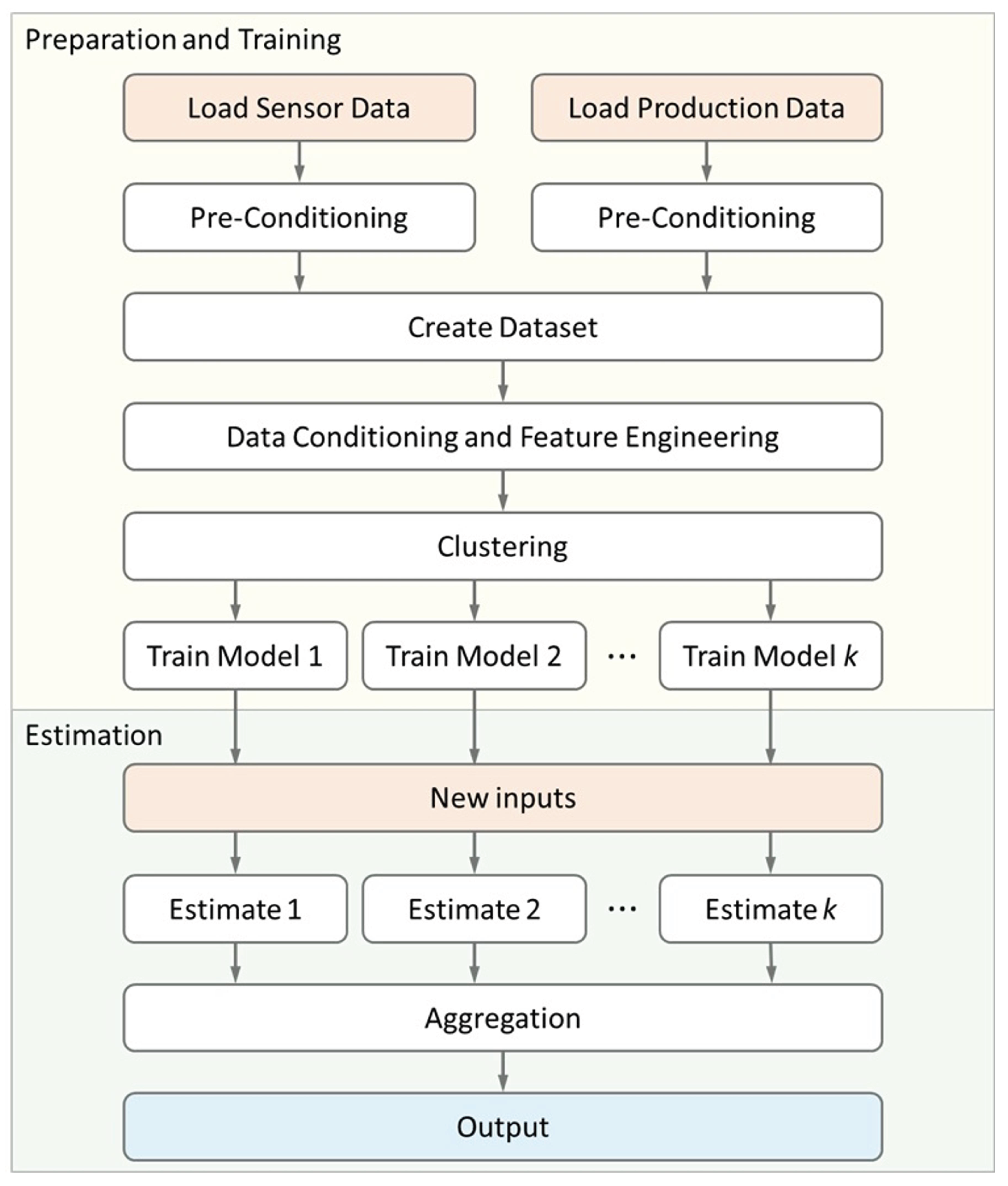
Figure 2.
Permanent Downhole Gauges (PDGs) positions in one-zone and two-zone well completion schemes.
Figure 2.
Permanent Downhole Gauges (PDGs) positions in one-zone and two-zone well completion schemes.
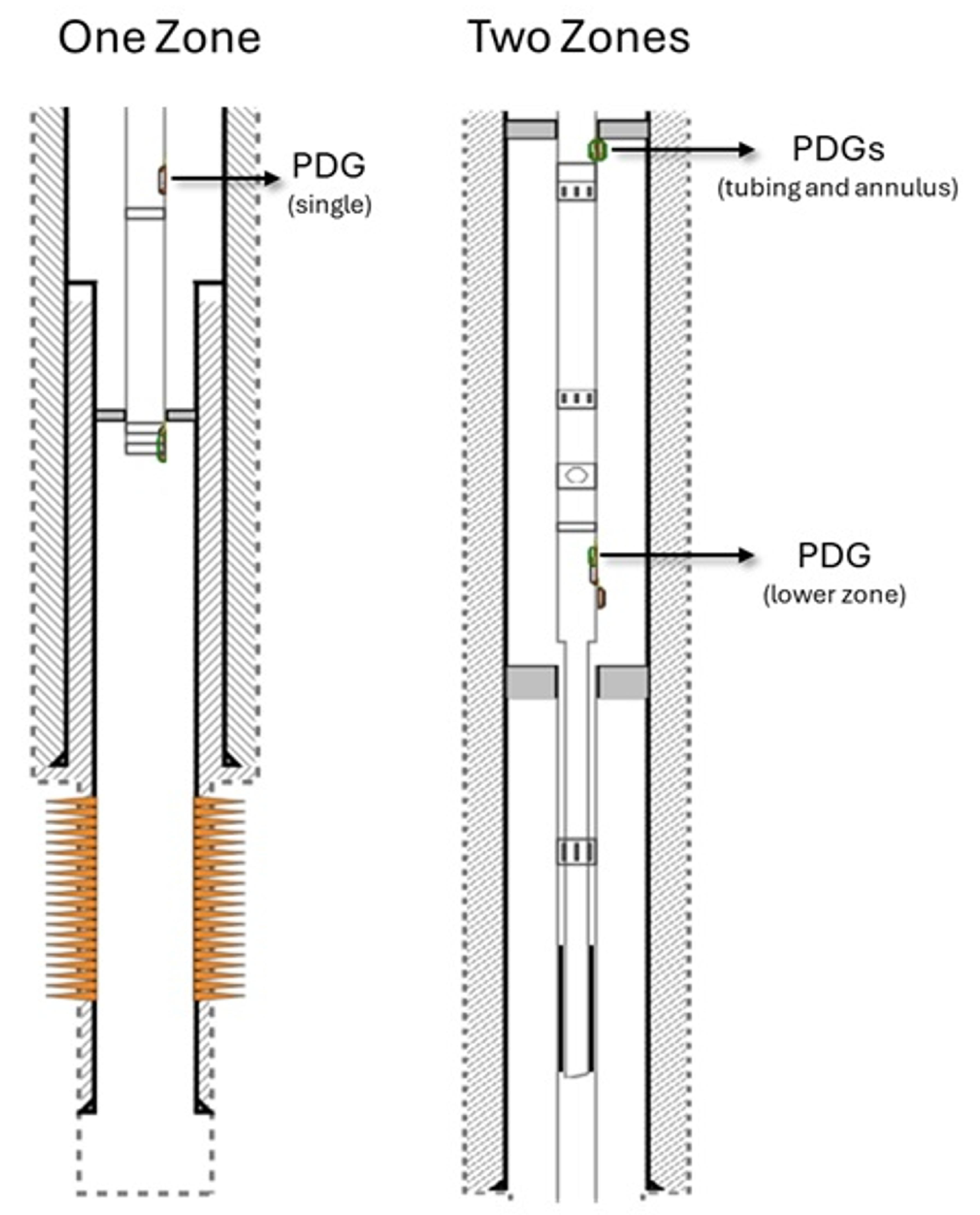
Figure 3.
Dataset partitioning process, reserving two different subsets for testing.
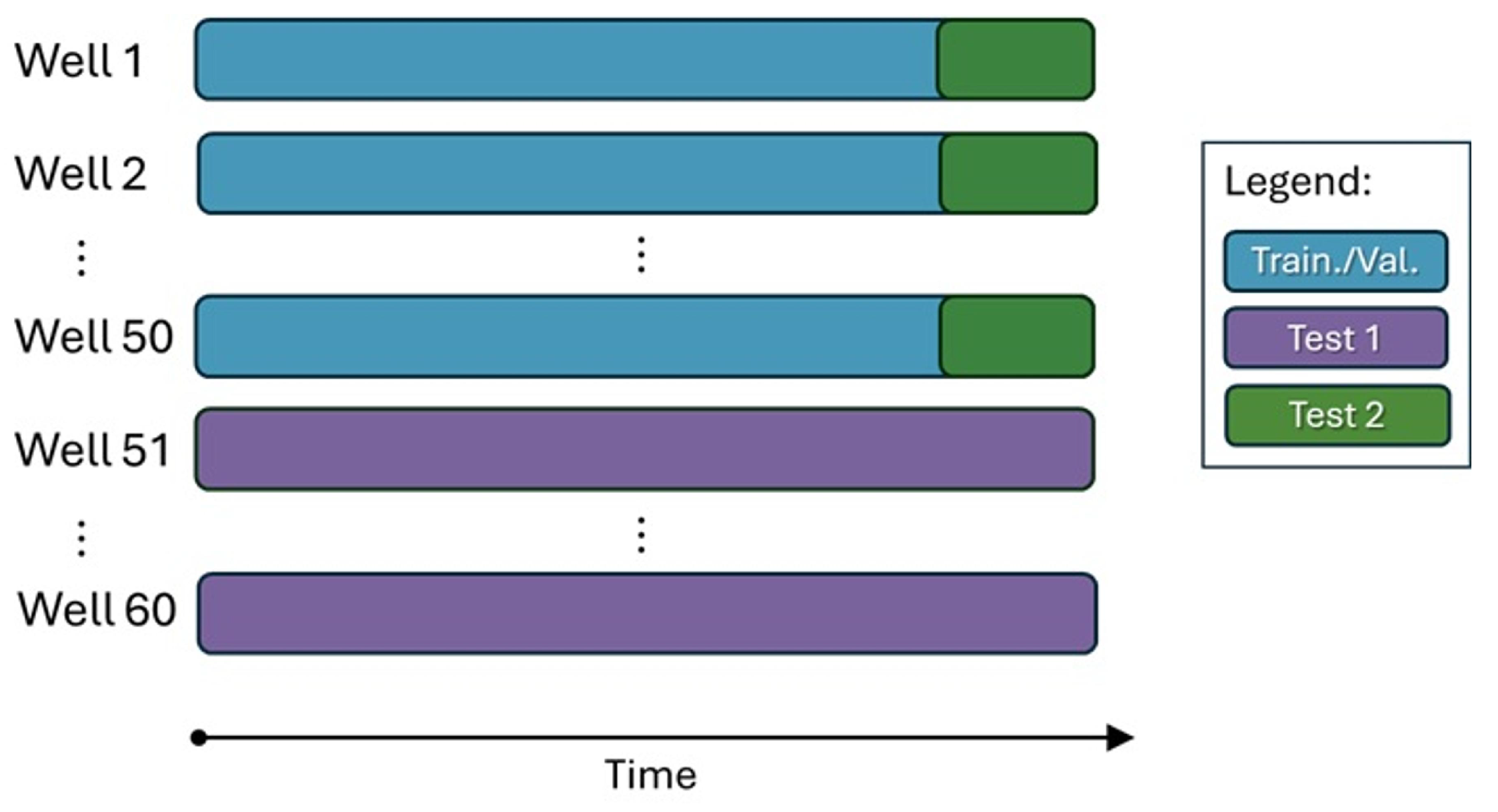
Figure 4.
Boxplots showing the probability distributions of the variables before outlier removal.
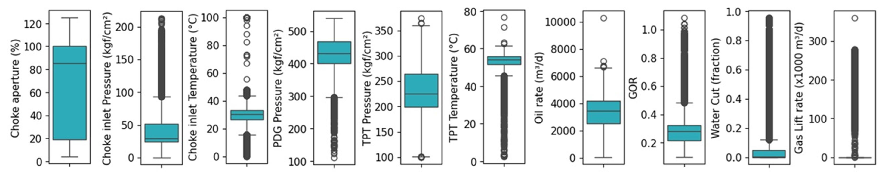
Figure 5.
Boxplots showing the probability distributions of the variables after outlier removal.
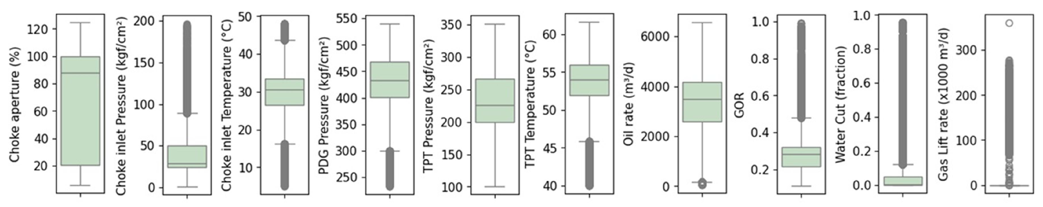
Figure 6.
Heatmap based on Pearson’s correlation coefficient for the variables of the problem, highlighting the output BHP.
Figure 6.
Heatmap based on Pearson’s correlation coefficient for the variables of the problem, highlighting the output BHP.
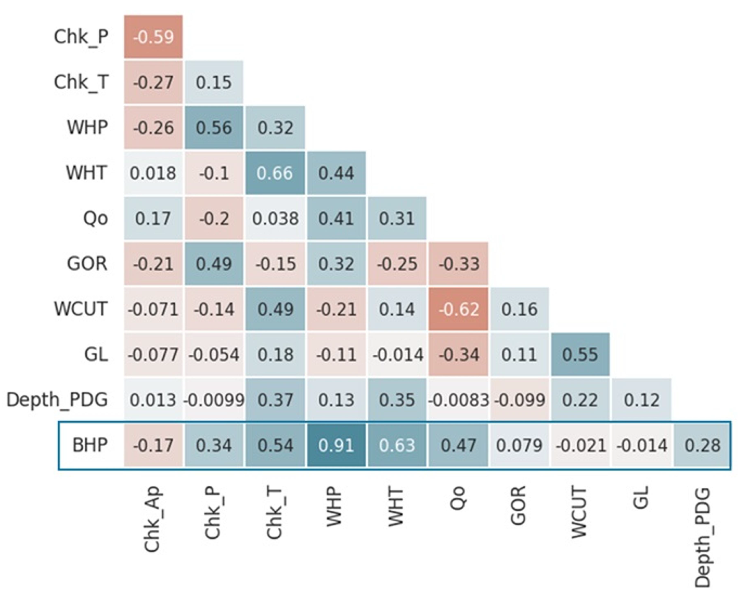
Figure 7.
Violin plots showing the probability distributions of the variables used in our study (normalized values).
Figure 7.
Violin plots showing the probability distributions of the variables used in our study (normalized values).

Figure 8.
Fuzziness parameter m and its influence in the memberships considering different distance ratios.
Figure 8.
Fuzziness parameter m and its influence in the memberships considering different distance ratios.
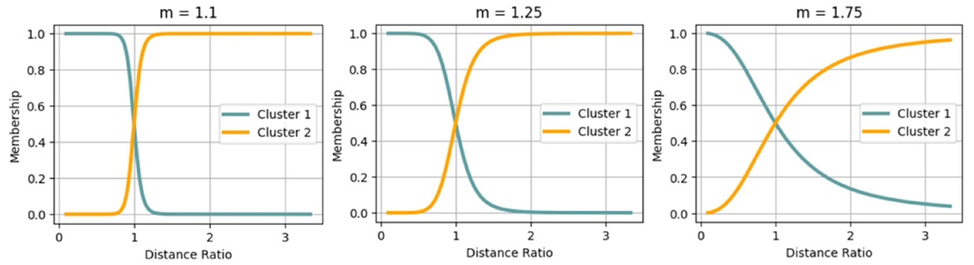
Figure 9.
Example of fuzzy memberships calculated for three clusters.
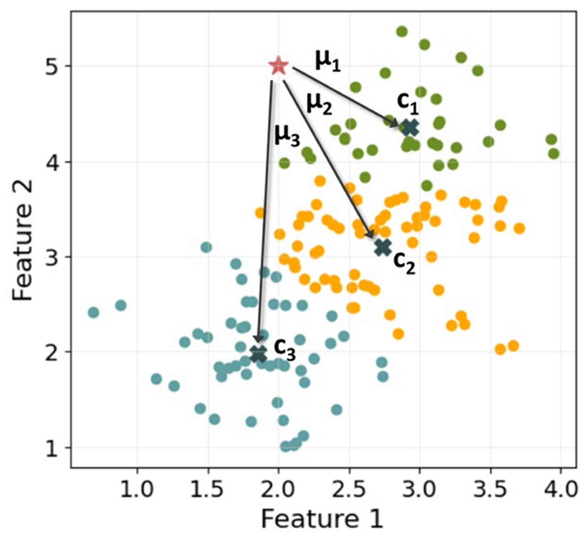
Figure 10.
Example architecture of a MLP Neural Network.

Figure 11.
Silhouette coefficients for different numbers of clusters for our dataset.
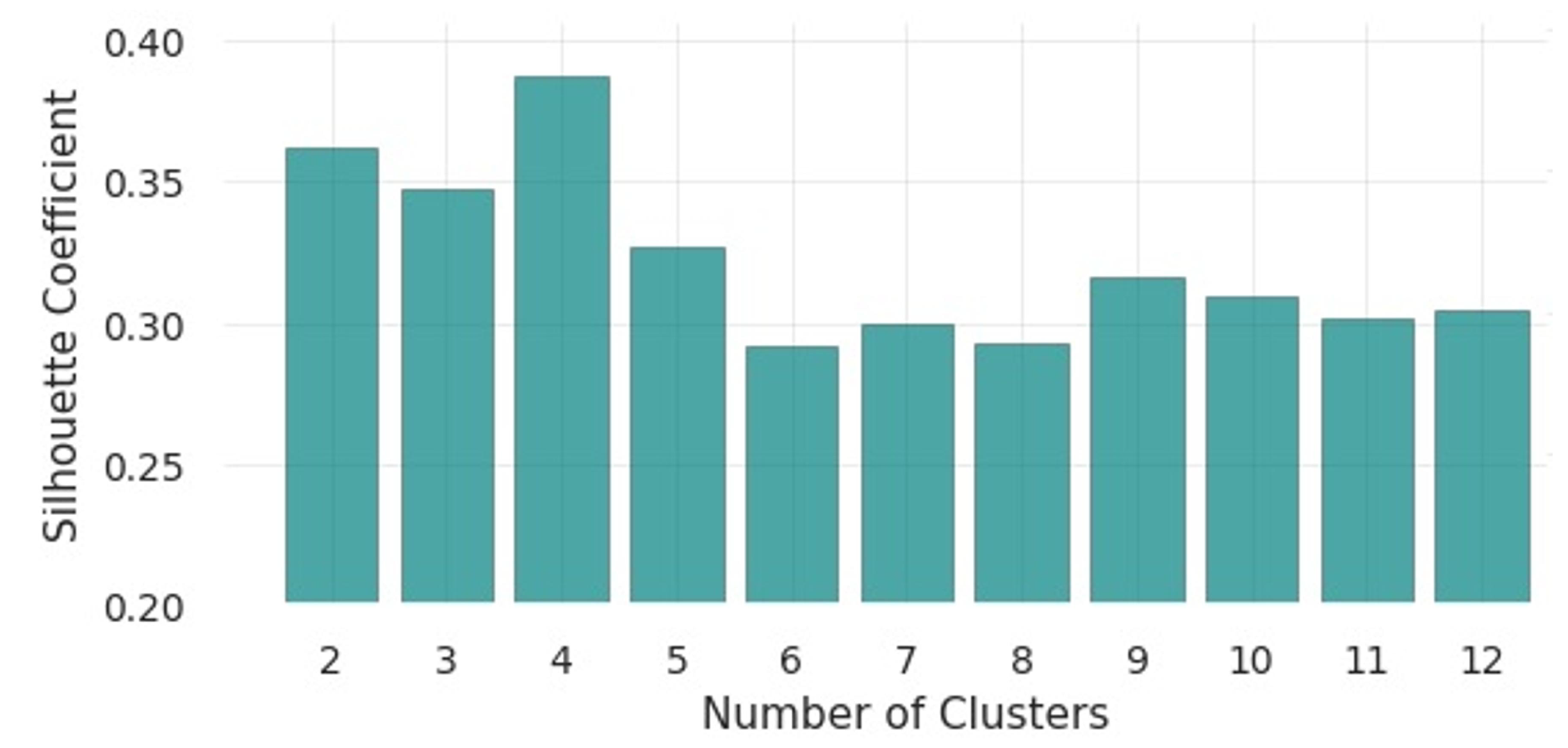
Figure 12.
Clustering for our dataset considering different numbers of clusters, plotted using dimensionality reduction illustrating the two principal components.
Figure 12.
Clustering for our dataset considering different numbers of clusters, plotted using dimensionality reduction illustrating the two principal components.
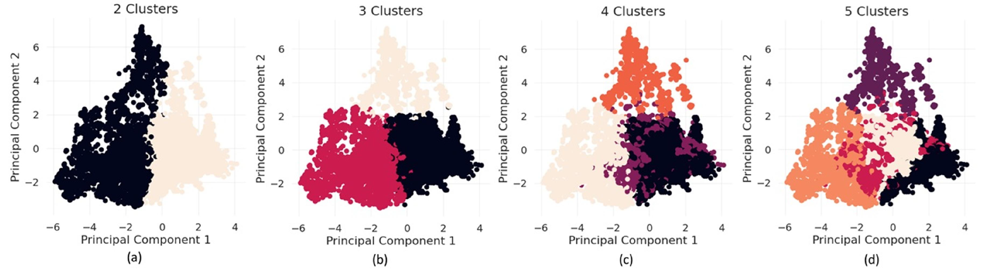
Figure 13.
Results for the model definition, showing MAPE from our three baseline ML models for the combinations of input sets and number of clusters.
Figure 13.
Results for the model definition, showing MAPE from our three baseline ML models for the combinations of input sets and number of clusters.
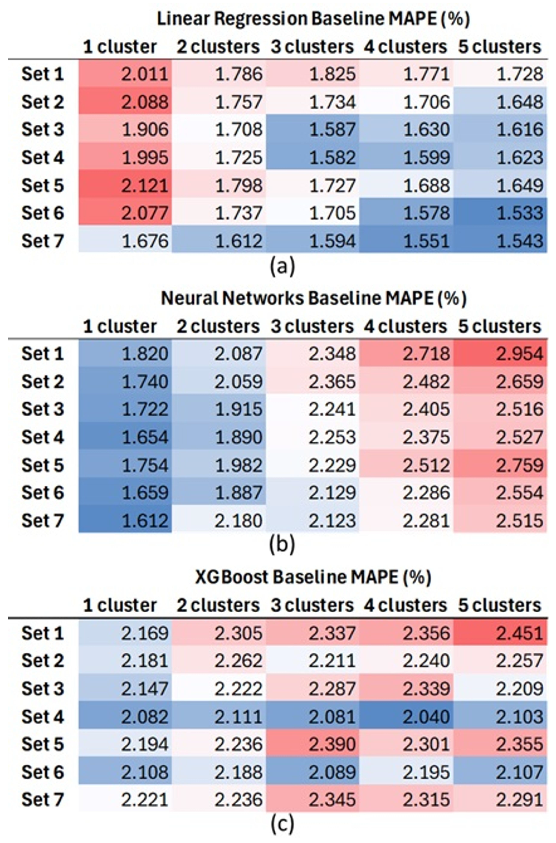
Figure 14.
Correlation of estimated versus actual values for the BHP from our best Linear Regression model.
Figure 14.
Correlation of estimated versus actual values for the BHP from our best Linear Regression model.
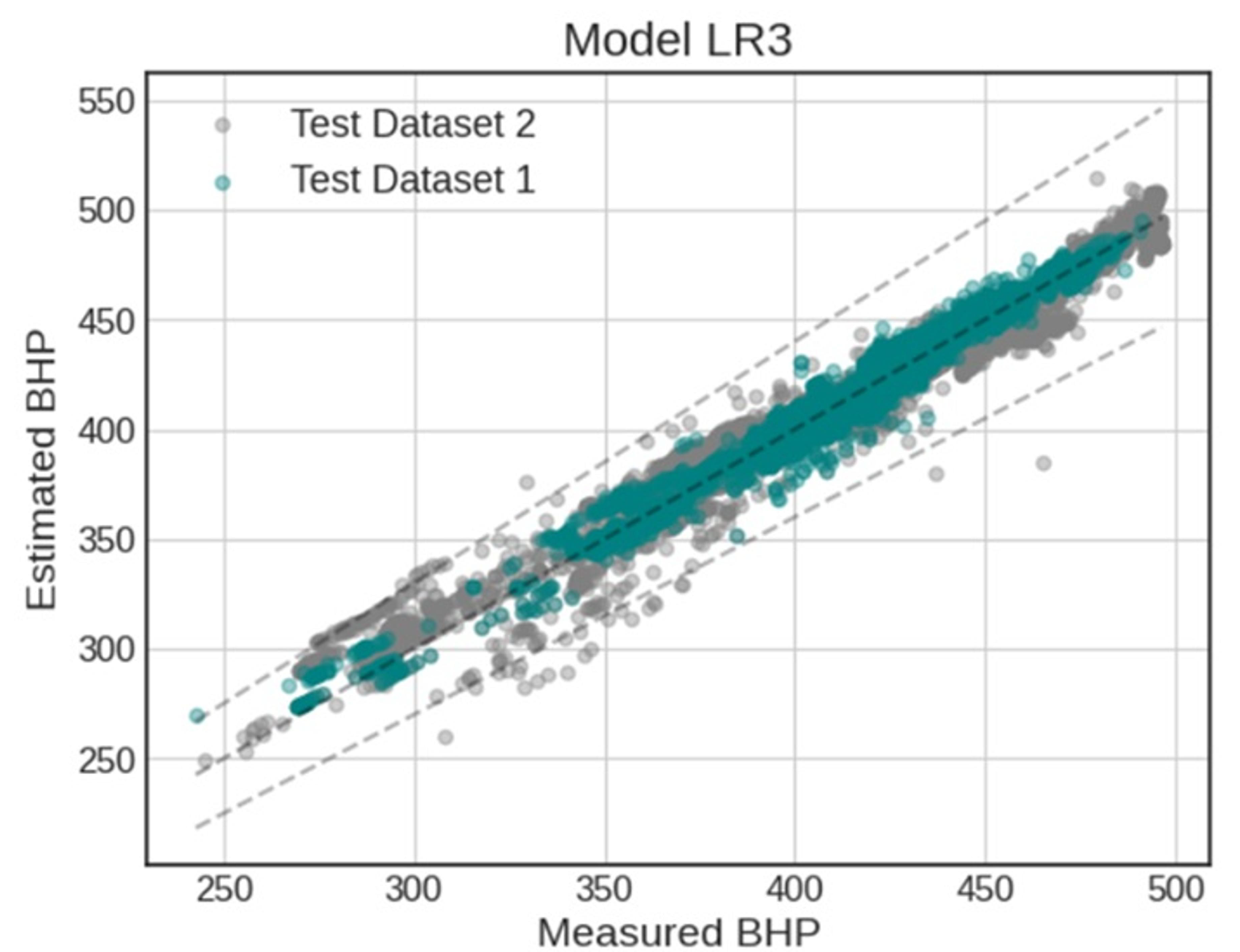
Figure 15.
Correlation of estimated versus actual values for the BHP from our best Neural Network model.
Figure 15.
Correlation of estimated versus actual values for the BHP from our best Neural Network model.
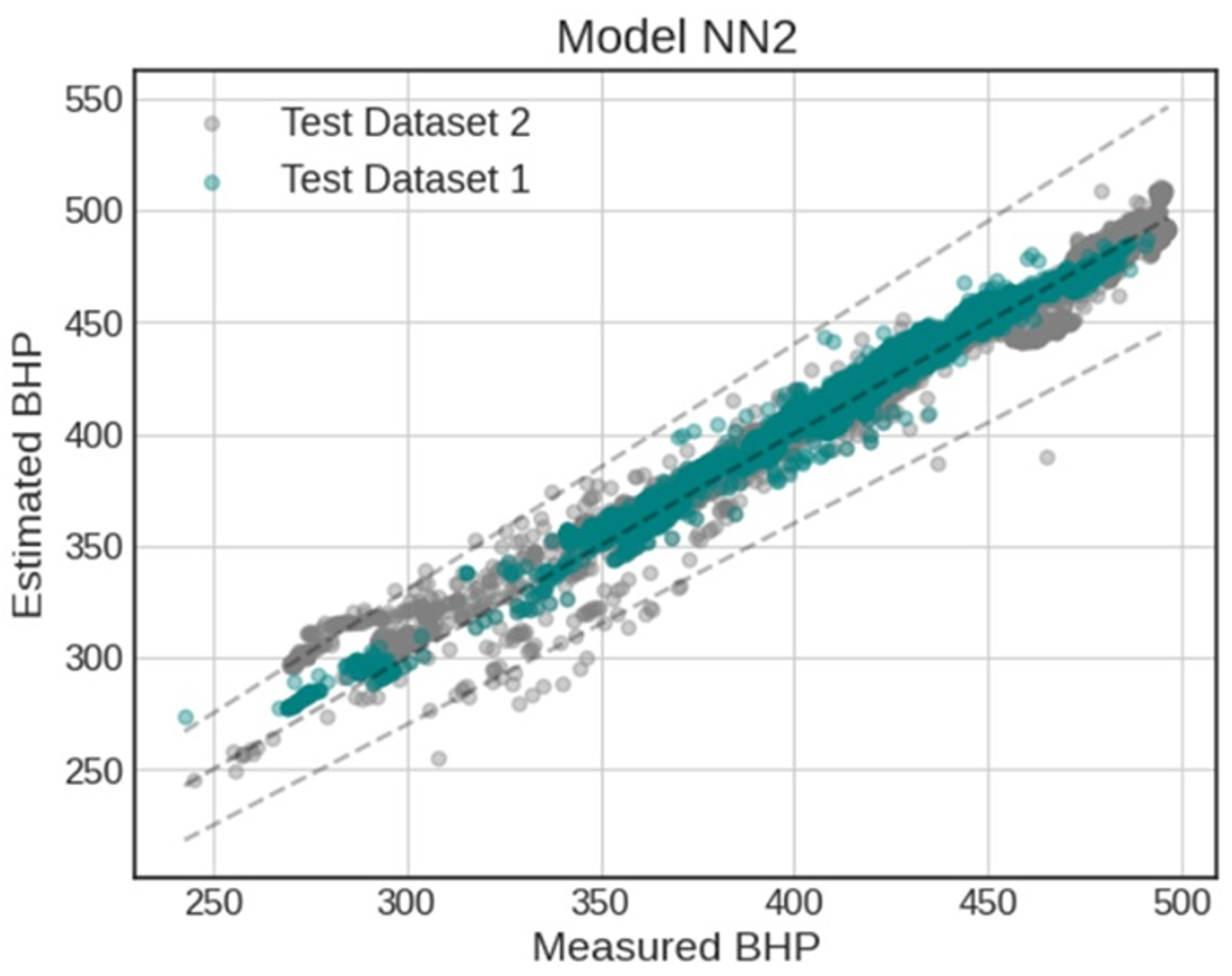
Figure 16.
Correlation of estimated versus actual values for the BHP from our best Gradient Boost model.
Figure 16.
Correlation of estimated versus actual values for the BHP from our best Gradient Boost model.
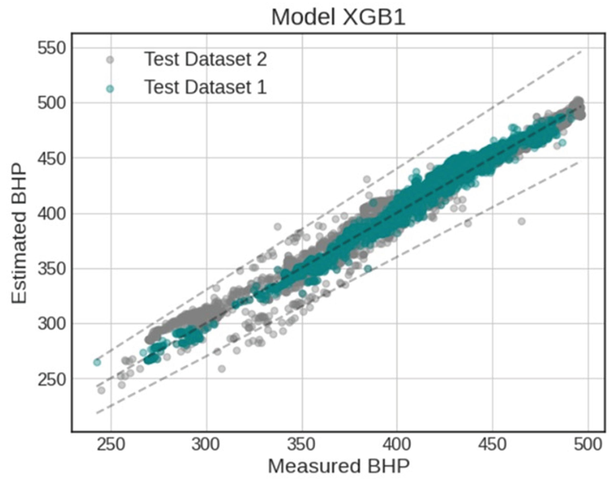
Figure 17.
BHP estimates with the three selected models, applied to a well with long production history.
Figure 17.
BHP estimates with the three selected models, applied to a well with long production history.
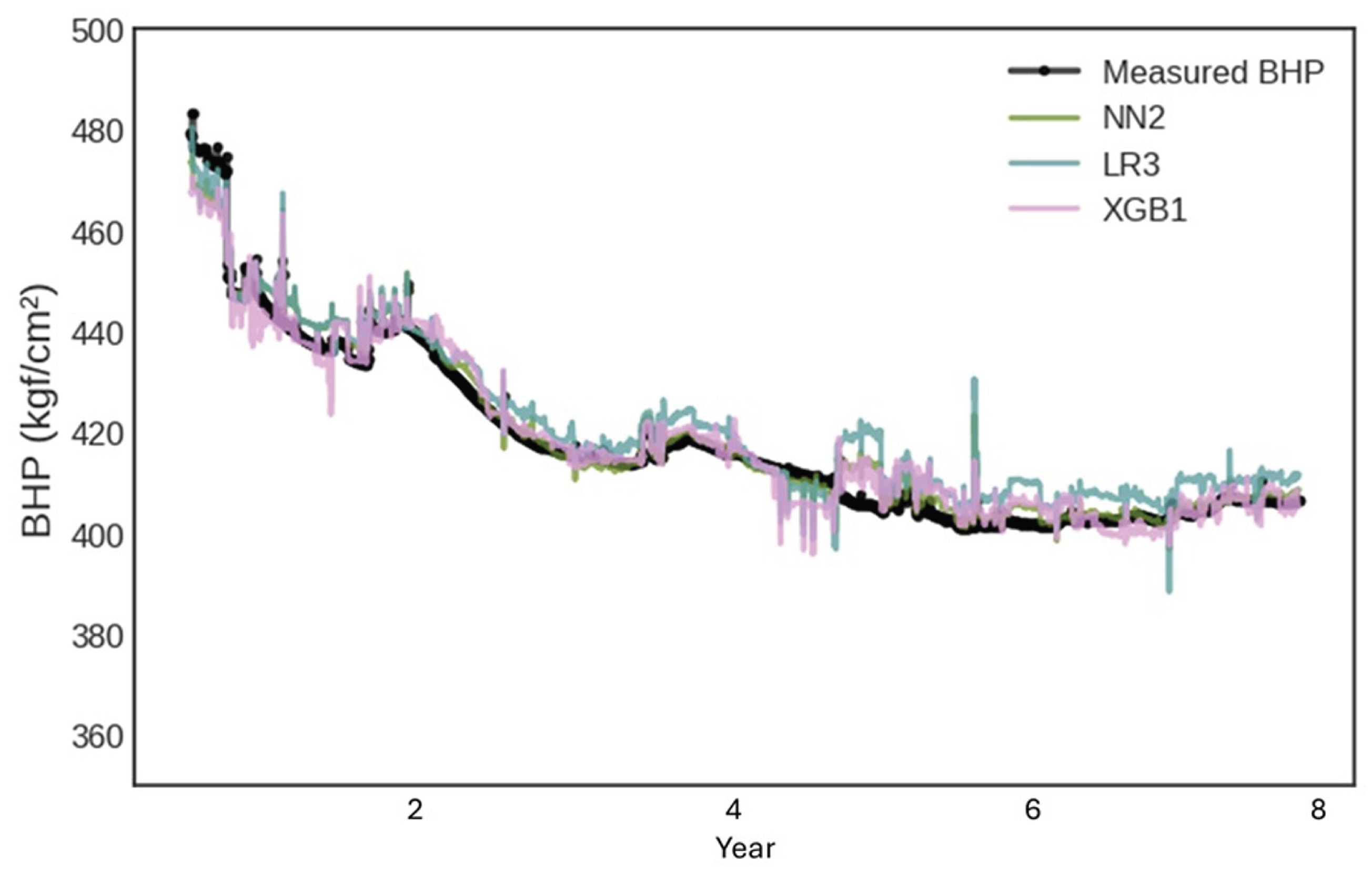
Figure 18.
BHP estimates with the three selected models, applied to a well with abrupt changes in production behavior due to ICV adjustments.
Figure 18.
BHP estimates with the three selected models, applied to a well with abrupt changes in production behavior due to ICV adjustments.
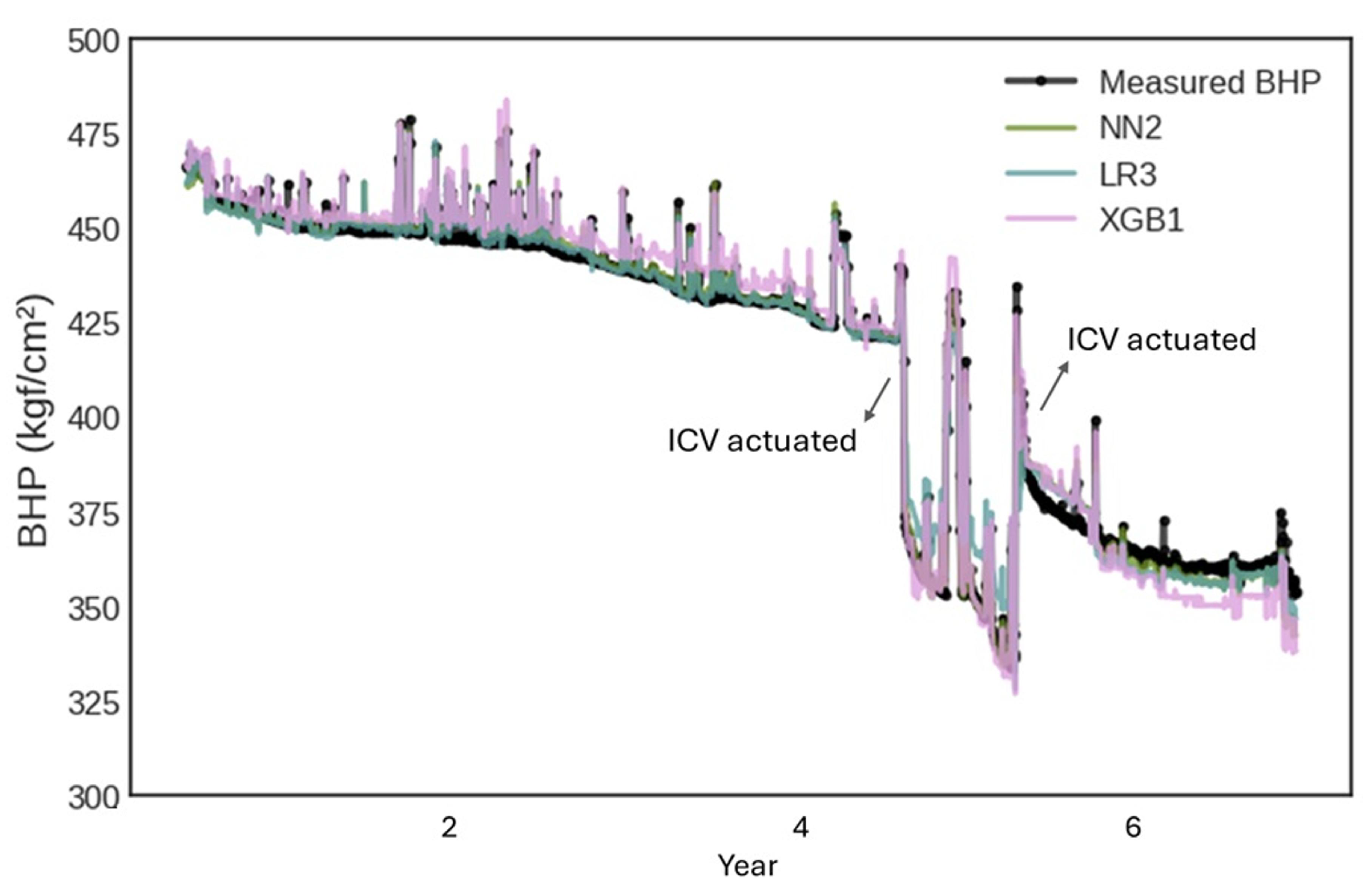
Figure 19.
BHP estimates with the three selected models, applied to a well whose production started after the training cutoff date.
Figure 19.
BHP estimates with the three selected models, applied to a well whose production started after the training cutoff date.
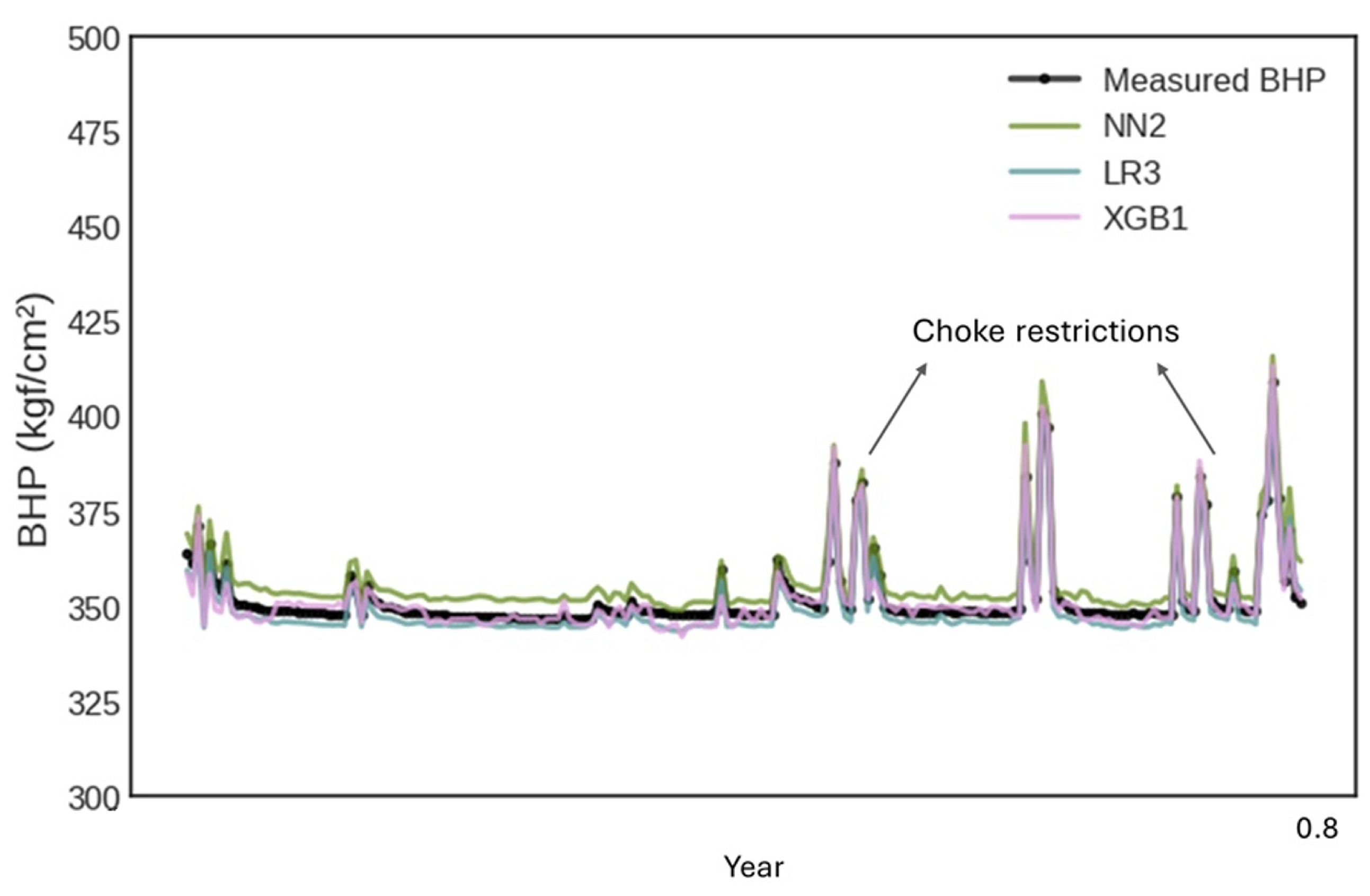
Figure 20.
Absolute error distribution by operating condition (boundaries) and estimator.
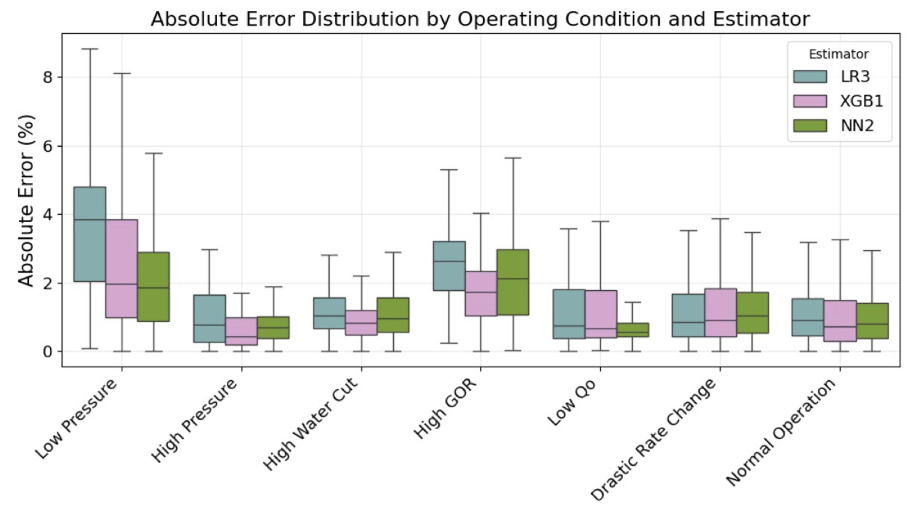
Figure 21.
Frequency distributions of BHP in the training and test datasets, relating to model performance.
Figure 21.
Frequency distributions of BHP in the training and test datasets, relating to model performance.
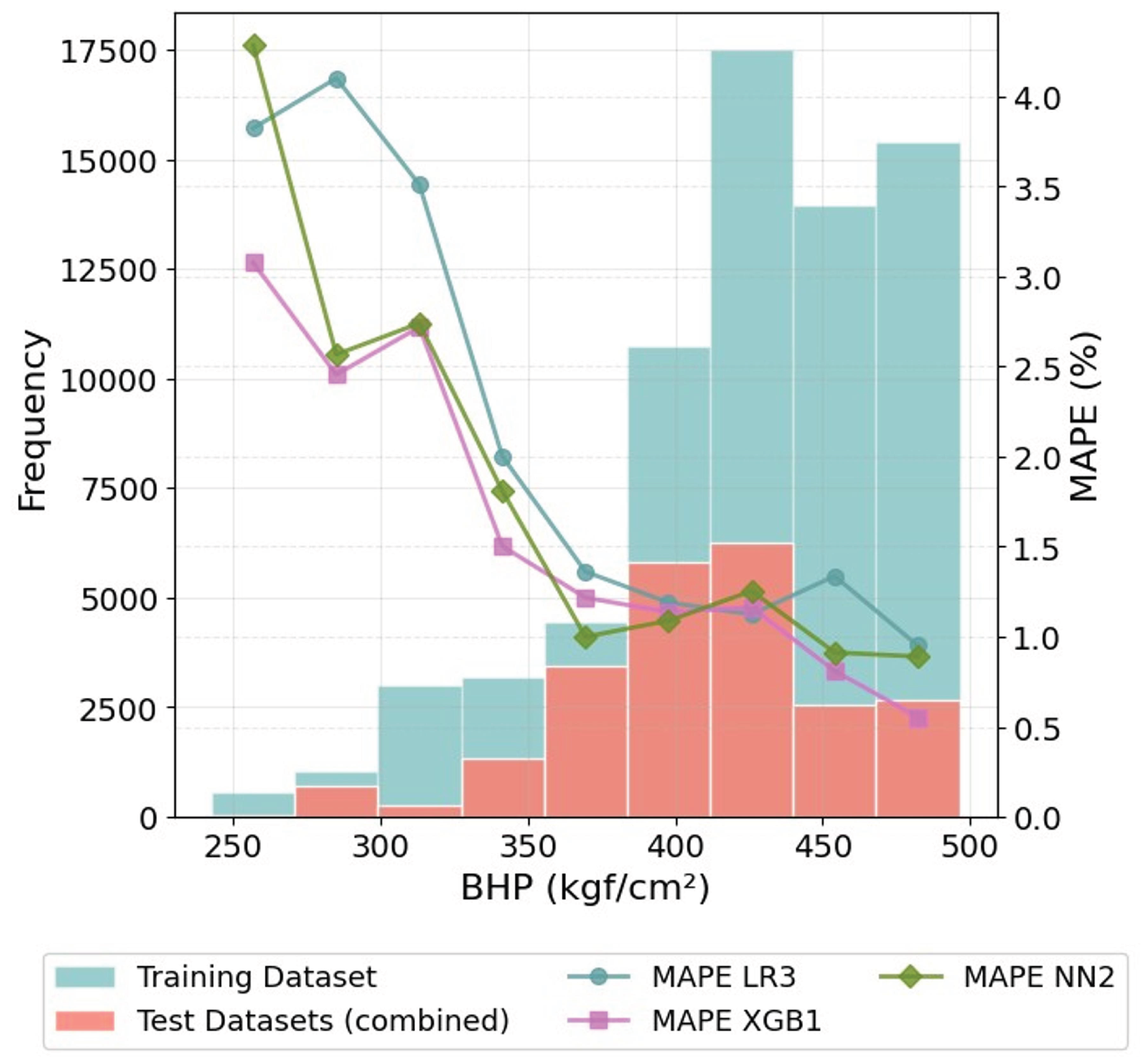
Figure 22.
BHP estimation during well testing, using data measured with frequency.
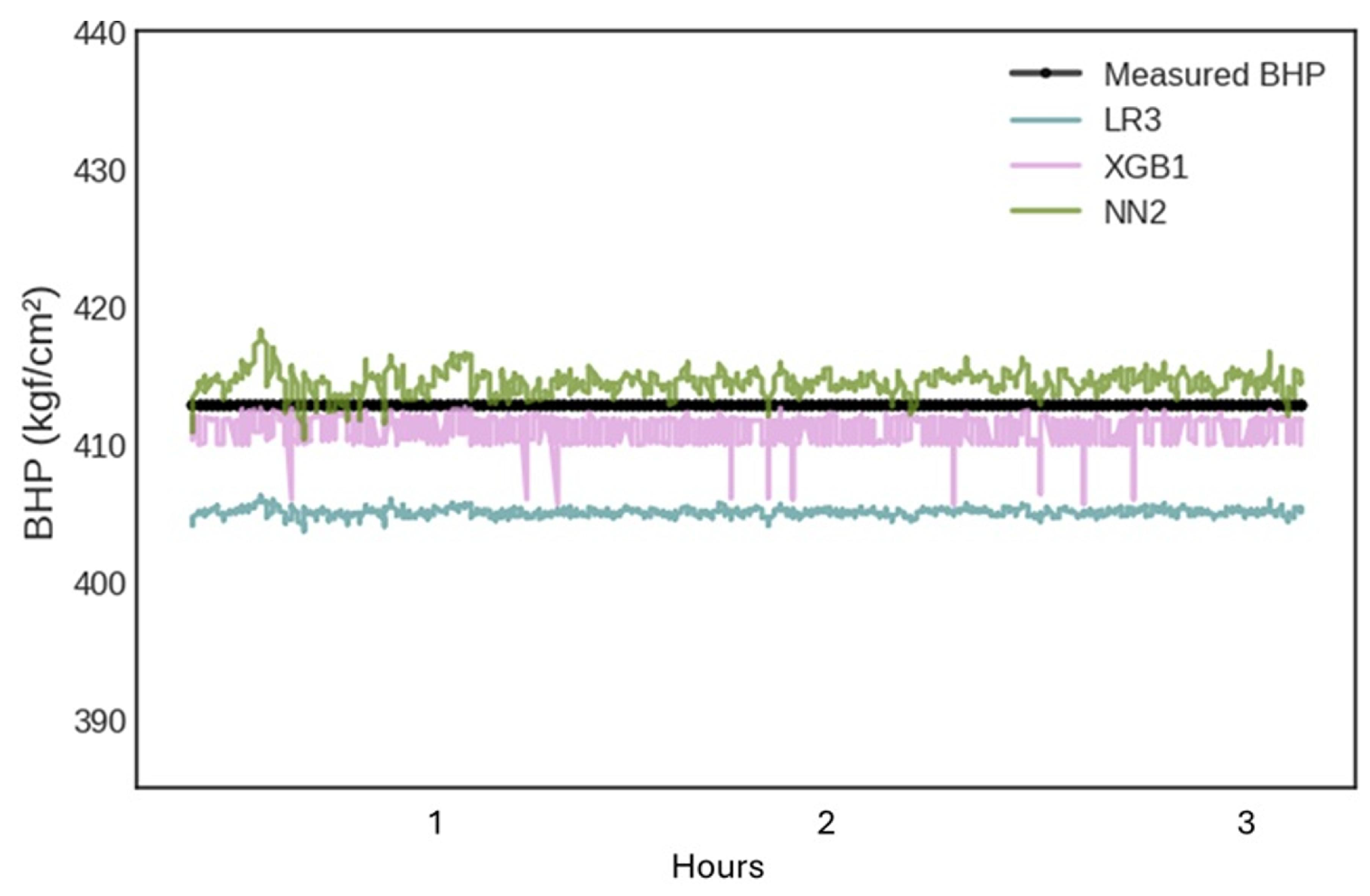
Figure 23.
Linear Regression Coefficients for the three clusters of our reference model LR3, for variable importance analysis.
Figure 23.
Linear Regression Coefficients for the three clusters of our reference model LR3, for variable importance analysis.
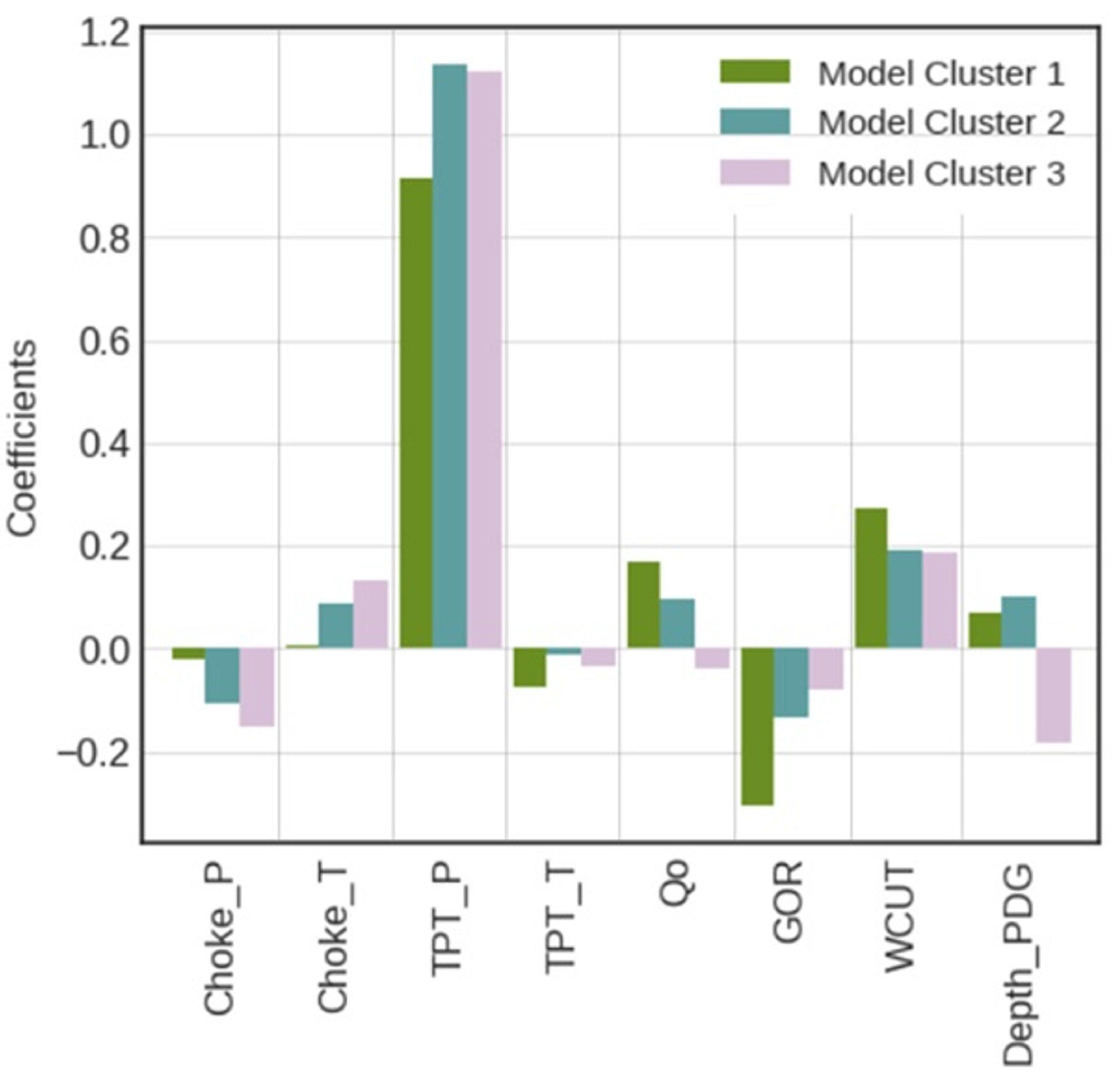
Figure 24.
Statistical distribution of the production parameters based on the training dataset.
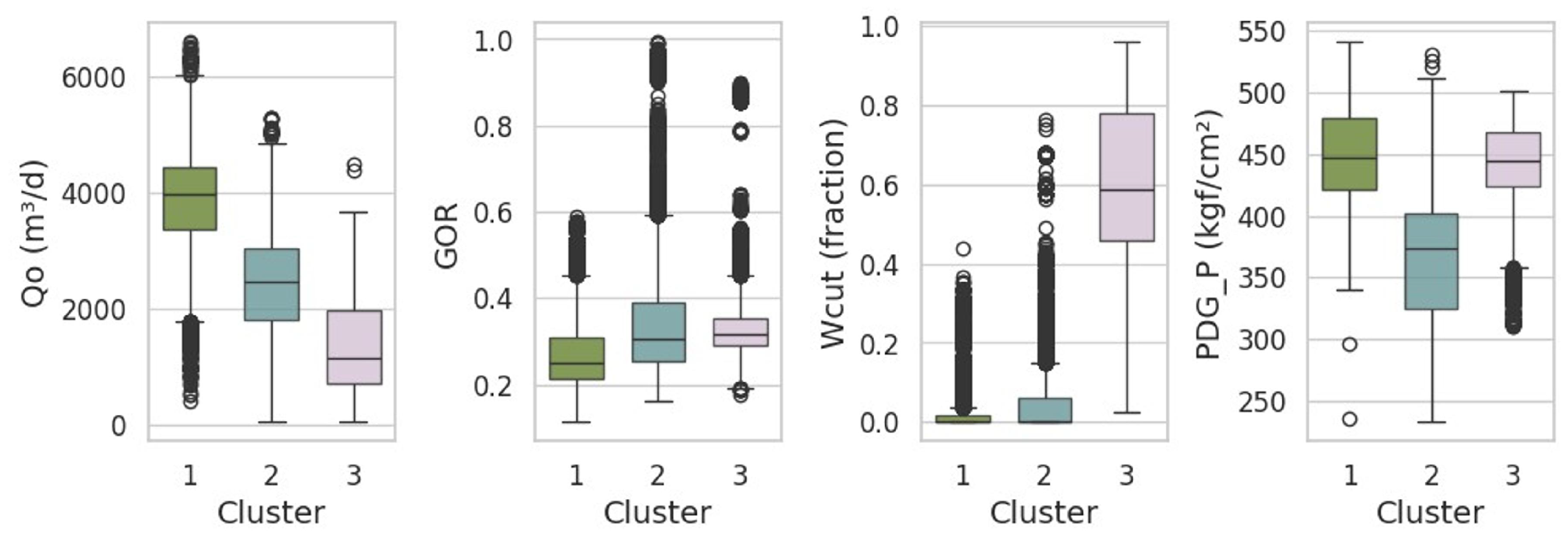

Table 1.
Statistical summary of the full dataset.
| Choke Ap | Choke P | Choke T | BHP | WHP | WHT | Qo | GOR | WCut | GL | Depth PDG | |
|---|---|---|---|---|---|---|---|---|---|---|---|
| (%) | (kgf/cm²) | (°C) | (kgf/cm²) | (kgf/cm²) | (°C) | (m³/d) | (m³/m³) | (fraction) | (Mm³/d) | (m) | |
| count | 107235 | 107235 | 107235 | 107235 | 107235 | 107235 | 107235 | 107235 | 107235 | 107235 | 107235 |
| mean | 63.36 | 44.46 | 29.87 | 421.76 | 225.14 | 53.2 | 3194.76 | 302.9 | 0.09 | 5.43 | 4825.67 |
| std | 39.12 | 32.86 | 8.19 | 55.3 | 49.77 | 4.11 | 1236.53 | 113.1 | 0.19 | 31.97 | 73.17 |
| min | 4.03 | 0 | 0.11 | 101.92 | 100.01 | 2.48 | 52.62 | 100.4 | 0 | 0 | 4547.5 |
| 25% | 20.34 | 24.05 | 25.83 | 395.95 | 196.21 | 51.47 | 2403.96 | 219.6 | 0 | 0 | 4787.9 |
| 50% | 85.86 | 29.18 | 30.21 | 426.44 | 222.63 | 53.67 | 3403.86 | 283.0 | 0 | 0 | 4834.1 |
| 75% | 100 | 51.3 | 33.3 | 464.21 | 258.62 | 55.75 | 4136.61 | 331.1 | 0.06 | 0 | 4881.2 |
| max | 125 | 214.14 | 100 | 540.67 | 375.34 | 76.77 | 10294.28 | 1438.6 | 0.96 | 373.58 | 4966.3 |
Table 2.
Statistical summary of training/validation dataset after outlier removal.
| Choke Ap | Choke P | Choke T | BHP | WHP | WHT | Qo | GOR | WCut | GL | Depth PDG | |
|---|---|---|---|---|---|---|---|---|---|---|---|
| (%) | (kgf/cm²) | (°C) | (kgf/cm²) | (kgf/cm²) | (°C) | (m³/d) | (m³/m³) | (fraction) | (Mm³/d) | (m) | |
| count | 73037 | 73037 | 73037 | 73037 | 73037 | 73037 | 73037 | 73037 | 73037 | 73037 | 73037 |
| mean | 64.15 | 44.15 | 29.89 | 427.76 | 228.76 | 53.66 | 3299.79 | 294.3 | 0.08 | 3.83 | 4831.9 |
| std | 38.97 | 32.33 | 6.79 | 53.17 | 49.59 | 3.23 | 1177.86 | 98.1 | 0.18 | 27.39 | 68.5 |
| min | 6 | 1.06 | 5.03 | 232.85 | 101 | 40.01 | 54.83 | 113.15 | 0 | 0 | 4547.5 |
| 25% | 20.38 | 24.16 | 26.51 | 401.32 | 199.57 | 51.93 | 2583.11 | 217.9 | 0 | 0 | 4796 |
| 50% | 88.23 | 29.13 | 30.54 | 433.38 | 225.56 | 54.06 | 3477.61 | 282.17 | 0 | 0 | 4834.1 |
| 75% | 100 | 50.25 | 33.37 | 468.92 | 265.76 | 55.97 | 4189.84 | 323.1 | 0.05 | 0 | 4884.9 |
| max | 125 | 196.82 | 48.1 | 540.67 | 351.28 | 61.7 | 6578.2 | 992.91 | 0.96 | 361.1 | 4966.3 |
Table 3.
Sets of input variables tested in the model definition.
| Set # | Input variables |
|---|---|
| Set 1 | [Choke P, Choke T, WHP, WHT, , , GL, Depth PDG] |
| Set 2 | [Choke P, Choke T, WHP, WHT, , , Depth PDG] |
| Set 3 | [Choke P, Choke T, WHP, WHT, , , , Depth PDG] |
| Set 4 | [Choke P, Choke T, WHP, WHT, , GOR, WCut, Depth PDG] |
| Set 5 | [Choke Ap, Choke P, Choke T, WHP, WHT, , , Depth PDG] |
| Set 6 | [Choke P, WHP, , GOR, WCut, Depth PDG] |
| Set 7 | [Choke P, WHP, , , WCut, Depth PDG] |
Table 4.
Configuration of the baseline ML models used in our preliminary definitions.
| ML Model | Parameters |
|---|---|
| Linear Regr. | [] |
| Neural Network | [layers = 1, neurons = 300, activation = ReLU, , dropout = 0] |
| XGBoost | [estimators = 500, max. depth = 5, learning rate , subsample = 0.95, , min. child weight = 20] |
Table 5.
Hyperparameters and their respective ranges evaluated in our Neural Network models.
| Parameter | Values (ranges) |
|---|---|
| Number of neurons | 30 to 300 |
| Dropout | 0.15 to 0.30 |
| Error function | MSE, MAE, SMAPE |
| Activation function | ReLU, GELU, ELU, Softplus |
Table 6.
Hyperparameters and their respective ranges evaluated in our XGBoost models.
| Parameter | Values (ranges) |
|---|---|
| Number of estimators | 100 to 1000 |
| Maximum depth | 4 to 10 |
| Minimum child weight | 8 to 32 |
| Learning rate | 0.1 |
| Subsample | 0.95 |
| Regularization factor | 0.1 |
Table 7.
Hyperparameters and their respective ranges evaluated in our LightGBM models.
| Parameter | Values (ranges) |
|---|---|
| Number of leaves | 16 to 64 |
| Maximum depth | 8 to 32 |
| Number of iterations | 300 to 1500 |
| Learning rate | 0.01 |
| Feature fraction | 0.90 |
| Bagging fraction | 0.80 |
| Bagging frequency | 5 |
| Maximum bins | 512 |
Table 8.
Results obtained with the most representative models for the 5-fold validation.
| Model | MAPE | SMAPE | nRMSE |
|---|---|---|---|
| LR1 | 1.533±0.659 | 1.532±0.658 | 2.093±0.840 |
| LR2 | 1.543±0.641 | 1.544±0.641 | 2.096±0.887 |
| LR3 | 1.582±0.753 | 1.582±0.757 | 2.068±0.903 |
| NN1 | 1.523±0.485 | 1.521±0.479 | 2.104±0.675 |
| NN2 | 1.530±0.521 | 1.527±0.513 | 2.127±0.782 |
| NN3 | 1.535±0.503 | 1.530±0.499 | 2.137±0.747 |
| XGB1 | 1.959±0.574 | 1.968±0.580 | 2.697±0.866 |
| LGB1 | 2.050±0.679 | 2.061±0.685 | 2.799±0.883 |
Table 9.
Results obtained with the most representative models for two blind test datasets.
| Model | Test Set 1 | Test Set 2 | ||||
|---|---|---|---|---|---|---|
| MAPE | SMAPE | nRMSE | MAPE | SMAPE | nRMSE | |
| LR1 | 1.296 ±0.001 | 1.304 ±0.001 | 1.572 ±0 | 1.346 ±0 | 1.349 ±0 | 1.839 ±0 |
| LR2 | 1.351 ±0.004 | 1.36 ±0.003 | 1.695 ±0.001 | 1.36 ±0.002 | 1.365 ±0 | 1.853 ±0 |
| LR3 | 1.166±0.005 | 1.171±0.005 | 1.451±0.003 | 1.468 ±0.001 | 1.472 ±0.002 | 1.937 ±0.004 |
| NN1 | 1.267 ±0.116 | 1.276 ±0.118 | 1.494 ±0.13 | 1.232 ±0.072 | 1.231 ±0.076 | 1.626 ±0.061 |
| NN2 | 1.302 ±0.13 | 1.311 ±0.133 | 1.506 ±0.136 | 1.182 ±0.135 | 1.182 ±0.059 | 1.569 ±0.063 |
| NN3 | 1.181 ±0.105 | 1.189 ±0.107 | 1.485 ±0.103 | 1.364 ±0.076 | 1.365 ±0.08 | 1.833 ±0.066 |
| XGB1 | 1.213 ±0 | 1.217 ±0 | 1.553 ±0 | 1.071±0 | 1.073±0 | 1.508±0 |
| LGB1 | 1.363 ±0 | 1.37 ±0 | 1.714 ±0 | 1.177 ±0 | 1.18 ±0 | 1.608 ±0 |
Disclaimer/Publisher’s Note: The statements, opinions and data contained in all publications are solely those of the individual author(s) and contributor(s) and not of MDPI and/or the editor(s). MDPI and/or the editor(s) disclaim responsibility for any injury to people or property resulting from any ideas, methods, instructions or products referred to in the content. |
© 2025 by the authors. Licensee MDPI, Basel, Switzerland. This article is an open access article distributed under the terms and conditions of the Creative Commons Attribution (CC BY) license (http://creativecommons.org/licenses/by/4.0/).
Copyright: This open access article is published under a Creative Commons CC BY 4.0 license, which permit the free download, distribution, and reuse, provided that the author and preprint are cited in any reuse.


