Submitted:
17 September 2025
Posted:
18 September 2025
You are already at the latest version
Abstract
As the penetration rate of distributed power sources increases and distribution network structures grow increasingly complex, the uncertainty in switch action control during load transfer has become a critical issue affecting grid safety and reliability. Traditional control methods based on precise probability-based predictive control are susceptible to bias introduced by prior settings under small-sample conditions, making it difficult to meet the stringent requirements of time-synchronized control. To address this, this study proposes an imprecise probability-based synchronous load transfer control method for distribution networks. By integrating the Imprecise Dirichlet model (IDM) with a Naive Credal Classifier (NCC), it constructs an interval predictive control model for switching action timing. This approach effectively mitigates the prior-dependency issue and enhances estimation robustness under small sample conditions. Combined with a dynamic delay strategy, this approach strictly controls the interval between disconnection and reconnection actions within 20 ms, preventing circulating current risks and ensuring transfer reliability. Simulation and experimental results demonstrate that the proposed method outperforms traditional Bayesian classifiers in both time prediction control accuracy and model robustness, providing a theoretical foundation and a reference for engineering applications for secure action control in distribution networks.
Keywords:
distribution network
; load transfer control
; imprecise probability
; naive credal classifier
; time control
; switch control action time
1. Introduction
The increasing penetration of distributed generation (DG) in distribution networks enhances flexibility while introducing uncertainty into system action control. Among these factors, the unpredictability of switching action timing during load transfer has become a critical determinant of grid security and supply reliability. Traditional control methods predominantly rely on precise probabilistic models (e.g., Bayesian classifiers) for timing prediction. However, under conditions of limited samples or insufficient prior information, such approaches are susceptible to subjective bias and struggle to meet stringent requirements for “open-then-close” sequencing and millisecond-level time synchronization control.
Imprecise probability theory characterizes uncertainty through interval probabilities, making it particularly suitable for inference scenarios with small samples or incomplete information [1]. In recent years, it has demonstrated significant advantages in fields such as reliability assessment and fault diagnosis. Against this backdrop, this paper proposes an imprecise probability-based load transfer control method for distribution networks. It integrates the Imprecise Dirichlet Model (IDM) with the Naive Credal Classifier (NCC) [2] to construct an interval prediction model for switch action times. This approach mitigates over-reliance on prior information [3] and enhances estimation robustness under small sample conditions [4].
This paper aims to systematically address the issue of insufficient time synchronization accuracy during load transfer control. By establishing a prediction model that better aligns with real-world uncertainties and incorporating a dynamic delay strategy, it achieves strict control of the switching time difference within 20 ms. This approach prevents circulating current risks and ensures transfer reliability. This research not only provides new theoretical support and a methodological framework for the safe action of distribution networks but also offers valuable insights for grid control under high penetration of renewable energy sources.
2. Literature Review
2.1. Research Status
With the advancement of new power system construction, the widespread integration of distributed generation (DG), energy storage devices, and flexible loads in distribution grids has made grid operation increasingly complex and dynamic. Traditional deterministic control methods struggle to address load synchronization and transfer issues under high uncertainty and small-sample scenarios. Against this backdrop, imprecise probability (IP) has gained increasing attention in both academic and engineering circles as a modeling tool capable of effectively capturing cognitive uncertainty and data scarcity.
Current research on load transfer control in distribution networks primarily focuses on optimization scheduling, intelligent algorithms, and reliability analysis. Traditional methods, such as control strategies based on Bayesian networks, Markov decision processes, or reinforcement learning, have enhanced system intelligence to some extent. However, under conditions of small sample sizes and high uncertainty, these approaches often suffer from issues like model overfitting and strong prior dependency.
To address these challenges, researchers have increasingly incorporated imprecise probability theory in recent years. Walley [5] systematically proposed a mathematical framework for imprecise probability, expressing uncertainty through upper and lower probability intervals to avoid the excessive reliance on a single prior characteristic of traditional probability models. Bernard [6] further introduced the Imprecise Dirichlet Model (IDM) to estimate probability intervals for multinomial distributions under small-sample conditions, significantly enhancing model robustness.
In classification and decision control, Zaffalon[7] introduced the Naive Credal Classifier (NCC), which employs credal sets to enable multi-class outputs for uncertain samples, effectively reducing misclassification risks. Corani & Zaffalon[8] validated NCC's superiority in small-sample classification within medical diagnostics, providing theoretical support for its application in power systems.
Regarding model architecture, Cozman [9] introduced Credal Networks, extending Bayesian networks into the domain of imprecise probability. This allows network nodes to represent probability intervals, making them suitable for inference and decision-making in highly uncertain environments. Masegosa & Moral[10] further explored integrating IDM with Credal Networks to learn uncertain probability models from small-sample data, offering novel insights for modeling distribution network control systems.
Although these studies are theoretically mature, their application in load synchronization transfer control for distribution networks remains nascent. Existing research primarily focuses on state estimation, fault diagnosis, or reliability analysis, while studies addressing load transfer path optimization and synchronous control strategy modeling under small-sample conditions remain relatively scarce. Therefore, exploring load synchronous transfer control methods based on imprecise probability not only represents theoretical innovation but also holds promising engineering application prospects.
2.2. Literature Summary
In summary, non-exact probability theory offers a novel research paradigm for load synchronization transfer control in distribution networks under conditions of small sample sizes and high uncertainty. This is achieved through methods such as upper and lower probability intervals, belief sets, and multi-prior fusion. IDM delivers robust probability estimates even under data scarcity, NCC significantly reduces misjudgment risks through multi-class outputs, while Credibility Networks extend traditional Bayesian topology to interval reasoning, endowing models with enhanced generalization capabilities and resilience. Looking ahead, as distributed generation penetration continues to rise, uncertainties across regions and timescales will intensify. Strategies based on imprecise probability—including online learning, rolling optimization, and multi-source information fusion—will become critical enablers for enhancing the resilience of distribution network control. These approaches hold significant theoretical value and broad engineering prospects for building secure, reliable, and intelligent new power systems.
3. Foundations of Imprecise Probability Theory Control
Based on the analysis of imprecise probability theory and its application advantages in Section 2, this study adopts the Imprecise Dirichlet Model (IDM) and the Naive Credal Classifier (NCC) as its core theoretical foundations. The following sections will elaborate on these approaches in detail.
3.1. Imprecise Dirichlet Model
The Imprecise Dirichlet Model (IDM) is an advanced Bayesian statistical approach for handling uncertainty, serving as an extension of the Dirichlet distribution [11] for estimating probability distributions under conditions of insufficient information. Consider a multinomial distribution with N possible outcomes, whose Dirichlet prior probability density function (PDF) is:
In the formula, θ=(θ1,θ2,…,θN)represents the probability of the result occurring, so that 0≤θn≤1 (n =1,2,…,N) and =1,α1, α2, …,αN represents the positive parameter of the Dirichlet distribution, andΓ(⋅)represents the gamma function, which is often used in statistics to represent the probability distribution of random variables.
Further, when the sample observation value M is obtained, the original prior Dirichlet probability density function is updated by Bayes' theorem. This updating process produces the posterior Dirichlet probability density function, which reflects the reevaluation of the parameters after taking into account the actual observed data[12]. The specific posterior probability density function form is shown in equation (2) :
In the formula,M={m1,m2,...,mn}is sample observation;mi represents the number of occurrences of the random variable state i. After obtaining the posterior probability density function, the parameter θn is estimated using the posterior distribution expected value, i.e
When analyzing the estimated results of a deterministic Dirichlet model, if observations are lacking, the probability θn of the n th result is determined by the parameter α, i.e., where the parameter α is called the prior weight of the result, often expressed as the parameter s, and is called the equivalent sample size in the Dirichlet distribution. In the probability estimation process, s represents the influence of prior distribution on posterior probability[13], that is, the larger the value of s, the more observed values are needed to adjust the parameters of prior distribution[14]. As shown in equation (3), one disadvantage of using the deterministic Dirichlet model is that when the available observations are small, the estimated results will be significantly affected by the prior distribution. If the setting is not reasonable, the estimated results based on the deterministic Dirichlet model may become inaccurate, thus affecting the final decision and prediction.
To overcome the shortcomings of the deterministic Dirichlet model, IDM uses a series of Dirichlet prior distributions instead of a single Dirichlet distribution. In IDM, the corresponding prior probability density function can be expressed as:
In the formula, rn (n = 1, 2, …, N)is the n th prior weight factor, and in equation (4) , s﹒rn has the same effect as αn. When rn varies within the interval [0,1], f(θ)will contain all possible prior PDFS for a given predetermined s, thus avoiding unreasonable effects of prior values.
Then, according to the updating process of Bayes' rule, a posterior PDF of the IDM relative to the observed value M can be calculated, which can be expressed as:
In the formula, represents the total number of observations.
Thus, a parameter representing the interval valued probabilities of all outcomes in the IDM, , , …, can be estimated from the posterior PDF by calculating the expected value, as follows:
The expected boundary shown in equation (6) is calculated with respect to the boundary of rn, namely 0 and 1[15]. Thus, the imprecise probability of random variable state occurrence in a given case can be estimated based on small sample data. The IDM statistical model eliminates the adverse effects of unreasonable prior Settings on event probability estimation in the absence of sample size.
3.2. Naive Credal Classifier
Naive Credal Classifier (NCC) is a classifier based on Naive Bayes (NB) that enhances the robustness of the model by introducing imprecise probabilities. The core idea of NCC is to provide more robust classification results by using a set of prior probabilities to model uncertainty in the face of incomplete or small-scale data sets, i.e. multiple possible categories can be returned in the face of uncertain instances. The Bayesian framework learns to update the prior with a profile representing the data evidence to calculate a posterior probability that can be used for decision making[16]. Formally, a classifier is a function that maps instances of a set of variables (called attributes or features) to the state or class of a class variable. The credal network uses the classical Bayesian network theory inference method to calculate the state value Xc of xc, and then by observing the specific value XE existing in the evidence variable xE, the probability P(xc|xE) can be calculated as follows:
In the formula, I is the number of multi-state random variables in the Bayesian network, P(xi|πi) is the conditional probability quality function, xi is the observation value of the i th random variable Xi, XiX, X represents all random variables in the network, πi is an observation value of Пi, which represents the state of the parent node of Xi, XM=X\(XEXc), represents a full probability operation on different states of variables in the node variable set XM.
Bayes classifiers perform classification by comparing the calculated posterior probabilities, and the category with the largest posterior probability is the classification result. However, when there is not a sufficient number of samples, Bayesian classifiers may return biased prior-dependent classification results, i.e. depending on the different priors employed, it may identify different classes as the most likely. However, any single a priori choice carries a certain arbitrariness, and these classifications are highly uncertain[17]. The credal network classifier relaxes the classification results of Bayesian classifiers by accepting imprecise probabilistic representations[18]. In a Bayesian classifier, each category of a class variable has a single-valued probability. In contrast, in a credal network classifier, the occurrence probability of each class can be expressed as an interval valued probability, that is, an imprecise precision probability.
In order to deal with the uncertainty of node random variables, the Credal Set (CS) concept is introduced into the credal network[19]. The credal set is used to describe the imprecise probabilistic properties of a node random variable, and mathematically, the credal set K(Xi) is defined as a closed convex set that covers all possible probabilistic mass functions P(Xi) of the random variable Xi. Specific definitions are as follows:
K(Xi) represents the closed convex set consisting of all possible probability mass functions P(Xi) of the random variable Xi, CH represents a convex hull, means that the sum of all possible probabilities must equal 1, and ΩXi is the range of values for Xi.
As shown in equation (9), there may be many combinations of prior distribution and observed data, so the credal set contains an infinite number of probability mass functions, but it only contains a finite number of extreme mass functions, which are called the vertices of the credal set, denoted as ext[K(Xi)]. These extremal functions correspond to the vertices that make up the convex hull, and they can be obtained by combining the endpoints of the probability interval. The classification of a credal network classifier consists of calculating the upper and lower bounds of the conditional probability of Xc=xc given XE=xE, a goal that can be achieved by calculating on a Bayesian network that corresponds to a limiting joint mass function as follows:
In the formula, P(X) represents the joint probabilistic mass function of all random variables, K(X) is the convex hull of a set of joint mass functions, i.e. the credal set, ext[K(X)] represents the limiting joint mass function of K(X), and P(X)∈ext[K(X)], which means that P(X) should be selected from ext[K(X)].
In this paper, IDM is used to model the prior, and it returns imprecise probabilities, which can be easily integrated into the credal network classifier, so as to realize the organic combination of IDM and credal classifier.
3.3. Naive Credal Classifier Classification Control Standards
Bayesian classifiers determine sample categories based on the principle of maximizing posterior probability in probability theory. Utilizing Bayesian networks, the classifier calculates the probability of each category by applying Bayes' theorem given known input evidence x. It then compares these probabilities and selects the category with the highest posterior probability as its classification decision. As shown in Figure 1, P(c1|x), P(c2|x) on the axis,... , P(c5|x) is calculated by a Bayesian classifier and the classification result is c1 because P(c1|x) has the greatest posterior probability.
Figure 2 and Figure 3 illustrate the diagnostic logic and output results of the credal network classifier. As shown in Figure 2, after computation, the Naive Credal Classifier category C1 as having a lower bound of posterior imprecise probability higher than all other categories. Consequently, C1 was designated as the sole diagnostic result under evidence condition X.However, in Figure 3, the lower limit of the posterior imprecision probability for C1 is lower than the upper limit of the posterior imprecision probability for C2, which indicates that the probability intervals of the two may overlap, as shown by the shaded area in the figure. In this case, the Naive Credal Classifier cannot determine an exact classification result, but instead provides a set of possible categories {C1,C2}, indicating that the sample is likely to be classified as C1 or C2 based on the conditions of evidence.
As can be seen, compared to Bayesian classifiers, the credal network controller provides a larger probability margin when performing category diagnosis on samples. When samples are unique, the credal network controller can deliver higher judgment reliability [19]. When faced with overlapping regions of maximum a posteriori imprecise probability intervals, the credal network controller can generate sets encompassing multiple possible categories, effectively reducing the risk of misdiagnosis.
4. Construction of a Switching Control Action Time Prediction Model Based on IDM-NCC
Based on the theoretical foundations of IDM and NCC described above, we now construct a credal network model for predicting switching action times in distribution networks.
4.1. Naive Credal Model for Switching Time Prediction in Distribution Networks
In power systems, the Point of Common Coupling (PCC) refers to the points where different power systems or power devices are connected to the main power grid, where the voltage and current can directly reflect the operating status of the distribution network system. By monitoring the voltage and current at the PCC, the action status of the distribution network can be effectively monitored. Compared with other complex electrical parameters, the three-phase voltage and current are relatively easy to measure and obtain, and can also help to monitor the stability of the power system. And in the distribution network, the distribution network switch needs to coordinate its action time according to the peak voltage and current to ensure that the power can be quickly and accurately cut off in the event of failure, so they become the preferred features for the implementation of switching time prediction and analysis. In this paper, the three phase voltage and three phase current peak value at PCC are taken as nodal evidence variables of the credal network, and the credal network is constructed.
Based on practical operational experience and relevant research, distribution networks exhibit a total of 12 operational states [20]. In this paper, utilizing Bayesian network theory and methodology, combined with conditions related to the time characteristics of distribution network switch actions, a credibility network classifier model was constructed to estimate the control action time of distribution network switches. As shown in Figure 4, this model provides a systematic approach for analyzing and predicting the time characteristics of switch actions within distribution networks.
In Figure 4, the parent node is the multi-state random variable of the switch action time of the distribution network, and F1~ F34 is set; The child nodes are the characteristic parameters E1, E2, E3, E4, E5 and E6 of the three-state random variables. For example, E1,1, E1,2, and E1,3 are good, good, and attention states of phase A current status, respectively. It can be seen that the model in this paper is a 2-layer credal network classifier, and the credal network classifier contains a parent node F, which is a multi-state query variable, that is, a 7-state random variable. The other 6 nodes are evidence variables representing the symptomatic attributes of the operating state of the distribution network. The typical switch time status classes and operational control symptom attribute sets for distribution networks are shown in Table 1 and Table 2.
Based on the established credal network structure, it is necessary to learn the conditional probability distribution of each evidence variable Ei under a given switch time state Fj from historical operational data. This paper employs the IDM model to accomplish this learning process, with the specific steps as follows: Using the proposed method to predict the action time characteristics of distribution network switch controls, first, for each switch time state class Fj (j=1,2,...,34), calculate the conditional credential set K(Ei|Fj) for evidence variable Ei under that state. For example, to obtain the conditional belief set K(E3|F2) for the phase-C voltage when the switching control action time is 5≤T<10 ms, we first calculate the imprecise conditional probabilities Pim(E3,1|F2), Pim(E3,2|F2), Pim(E3,3|F2), i.e.,
In the formula, N represents the number of times in which the status of distribution network switch control action time is F2 within the statistical period of distribution network action; n3,1, n3,2, n3,3 respectively represent the number of times when the C-phase voltage status of the distribution network switch control action time state is good and good respectively under the condition of F2; s is the parameter set in the IDM, and the value in this paper is 1[21].
Furthermore, the credal set K(E3|F2) is obtained, i.e
In the formula, The probability mass function K(E3|F2) in the credal set K(E3|F2) takes a value in the upper and lower boundary range of its corresponding imprecise probability.
In this case, the vertex of the credal set ext[K(E3|F2)] can be determined using the inexact probability upper and lower bounds corresponding to the credal set K(E3|F2), i.e. :
For other conditional credal set K(Ei|Fj)(i=1,2,3,...,6, j=1,2,3,...,34), the procedure is the same as K(E3|F2).
4.2. Model Solving and Classification Output Process
Then, on the basis of obtaining the conditional reliability set K(E1|F), K(E2|F), ..., K(E6|F), the posterior imprecise probability of each switch action time state of the distribution network under the condition of obtaining the attribute state of the distribution network can be solved according to the accurate reasoning algorithm of the credal network shown in equations (8) and (9), as shown in equation (14).
Finally, after obtaining the known Pim(F|Ei), according to the classification criterion of the credal network classifier, the predictive results of switching action time characteristics of the distribution network are output.
The imprecise conditional probability control estimation process of switching action time of distribution network described in this paper is shown in Figure 5.
5. Example Analysis
5.1. Model Solving and Classification Ooutput Process
This paper investigates switch timing prediction methods for distribution networks incorporating distributed generation (DG) under various operational conditions, using a double-fed distribution network as an example. A microgrid model incorporating distributed photovoltaic generation was constructed. The distribution system operates at a reference voltage of 10.5kV, with all lines configured as overhead lines. Unit resistance and reactance were set as: R=0.26Ω/km, X=0.355Ω/km, for line lengths of 3km, 3km, and 10km respectively. Both Feeder 1 and Feeder 2 terminate with a load capacity of 6 MVA and a power factor of 0.85. The DG output power is adjustable within the range of 0–10 MW. A distribution network switch is installed at the PCC to detect the switching on and off times of the distribution networkThe simulation is carried out for different working conditions of the distribution network. The specific situation is as follows: the three-phase voltage and three-phase current at PCC under each working condition are collected. The feature data of each operating condition can be formed into a feature vector with a dimension of 1×6, considering that there are 310 different operating conditions, these data can be combined into a feature matrix of 310×6 dimensions. In order to eliminate the influence of different dimensions, it is necessary to normalize the eigenmatrix. Using the discrete standardization method, the eigenvalues of S1-S310 can be converted to the valid range of [0,1]. Take S1 as an example, the normalization process follows the following method :
In the formula, Ei and are the values before and after the normalization of the attributes of the i th operating state symptom respectively; Emax and Emin are the maximum and minimum values of Ei. The same is true for S2~S310. The normalized database is shown in Table 3.
The normalization of the feature matrix involves six indicators of each operating condition in the database, which together form a feature vector. 310×80%=248 feature vectors were randomly selected from the database as the training data set, and the remaining 310×20%=62 vectors were selected as the test data set. The imprecise probability estimation method is used to predict and analyze these data.
5.2. Case 1: Unique Category Output Results and Analysis
In Case 1, the case where the credal network classifier gets a single unambiguous result at the time of diagnosis is chosen, where the state of the evidence variable is represented as vector S1. Then, according to these evidences, imprecise probability estimation method and Bayesian classifier are used to predict the operation time (or total action time) of the distribution network switch respectively, and the prediction results are shown in Table 4 and Table 5.
Table 5 shows the prediction results of the Bayesian classifier, in which the distribution network switching time state class F30 has the highest probability of a posterior single value, so the switching time range predicted by the Bayesian classifier is between 38ms and 39ms. Furthermore, according to the data in Table 4, the lower bound of the imprecise probability Pim(F30|S1) calculated using the method described in this chapter exceeds the upper bound of all other posterior imprecise probabilities. This shows that the credal network classifier can also derive the same uniqueness class F30 as the Bayesian classifier, and the prediction results of both are consistent.
Through the above analysis, we can conclude that Case 1 proves that the non-precise probability-based distribution network switching time prediction method proposed in this paper shows the same prediction efficiency as traditional prediction methods (such as Bayesian classifier) when dealing with the mapping relationship between distribution network detection test data and operating state.
5.3. Case 2: Similarity Set Output Results and Analysis
In Case 2, the prediction result of the credal network classifier is a similar set of classes, and the results are shown in Table 6.
In order to compare with the method proposed in this chapter, this paper also uses Bayesian classifier to predict it, and the results are shown in Table 7.
By analyzing Table 7, it can be seen that the switching time state class F23 of the distribution network has the largest probability of a posterior single value, which results in the switching time predicted by the Bayesian classifier to be between 31ms and 32ms. However, according to the analysis in Table 6, according to the diagnostic criteria of credal network classifiers, the proposed method will output a similar set of classes {F22, F23} with a predicted switch control action time range of 30ms to 32ms. Further inspection confirmed that the actual operating time of the distribution network switch was 30ms.
Case 2 shows the limitations of traditional control forecasting methods in the prediction of switch control action time of distribution network. In contrast, the imprecise probability-based method proposed in this paper can effectively avoid prediction errors by providing outputs of similar sets. The actual test results prove that this method based on imprecise probability is effective in predicting the operation time of the distribution network switch, which is of great significance for enhancing the stability of the distribution network switch and optimizing the operation of the power network.
6. Time-Based Model for Whole-Process Control and Experimental Validation
The construction of a time-dependent model for load transfer in distribution networks requires a multidimensional characterization of temporal coupling relationships across all stages. This involves both quantifying the cumulative effects of deterministic processes and analyzing the propagation patterns of random factors. The model's core objective is to accurately predict the total time control interval from the issuance of the master station command to the final switch operation, while ensuring compliance with “open-then-close” sequencing and time-difference constraints even under extreme scenarios. By integrating mathematical modeling with engineering experience, we can systematically evaluate the boundary conditions of time parameters and their impact mechanisms on the overall process, providing theoretical support for control strategy design. This strategy requires, based on precise time synchronization, that the time interval from complete disconnection to complete reconnection be within 20 milliseconds, disregarding communication time from the master station to the terminal.
6.1. Time Constraints and Pproblem Modeling
Target: Total time (interval from trip completion to close completion) must satisfy0 <Ttotal< 20ms.
Known Conditions:
Closing time Ton > Opening time Toff, but specific values are unknown.
Master Station Command Sequence:
t0: Issue closing command
t0 +Δt: Issue opening command
Mathematical Model
Opening completion time: toffend = t0 + Toff
Closing completion time: tonend = t0 + Ton+ Δt
Total time constraint: Ttotal = tonend - toffend and 0 < Ttotal < 20ms
6.2. Control Strategy Design: Determination of Dynamic Delay Time Δt
Constraint Derivation:
Disconnection completion must precede reconnection completion (to prevent parallel circulating currents):
toffend < tonend △t < Ton -Toff
Total Time Constraint:
0 < Ttotal < 20ms →Toff -Ton <△t < Toff -Ton+20
Safety Margin Determination:
If nominal values of Ton and Toff are known:
△t = Ton - Toff - 10ms (take midpoint value, reserve 10ms margin)
If parameters are unknown, calibration via experimentation is required:
Step 1: Measure typical values of Ton and Toff in the laboratory.
Step 2: Set △t = Ton - Toff - 10ms and verify that Ttotal ∈ (0, 20) ms.
6.3. Physical Experiment Verification and Result Analysis
Test scenario
Figure 6.
Distribution network load synchronous transfer control time accuracy test.
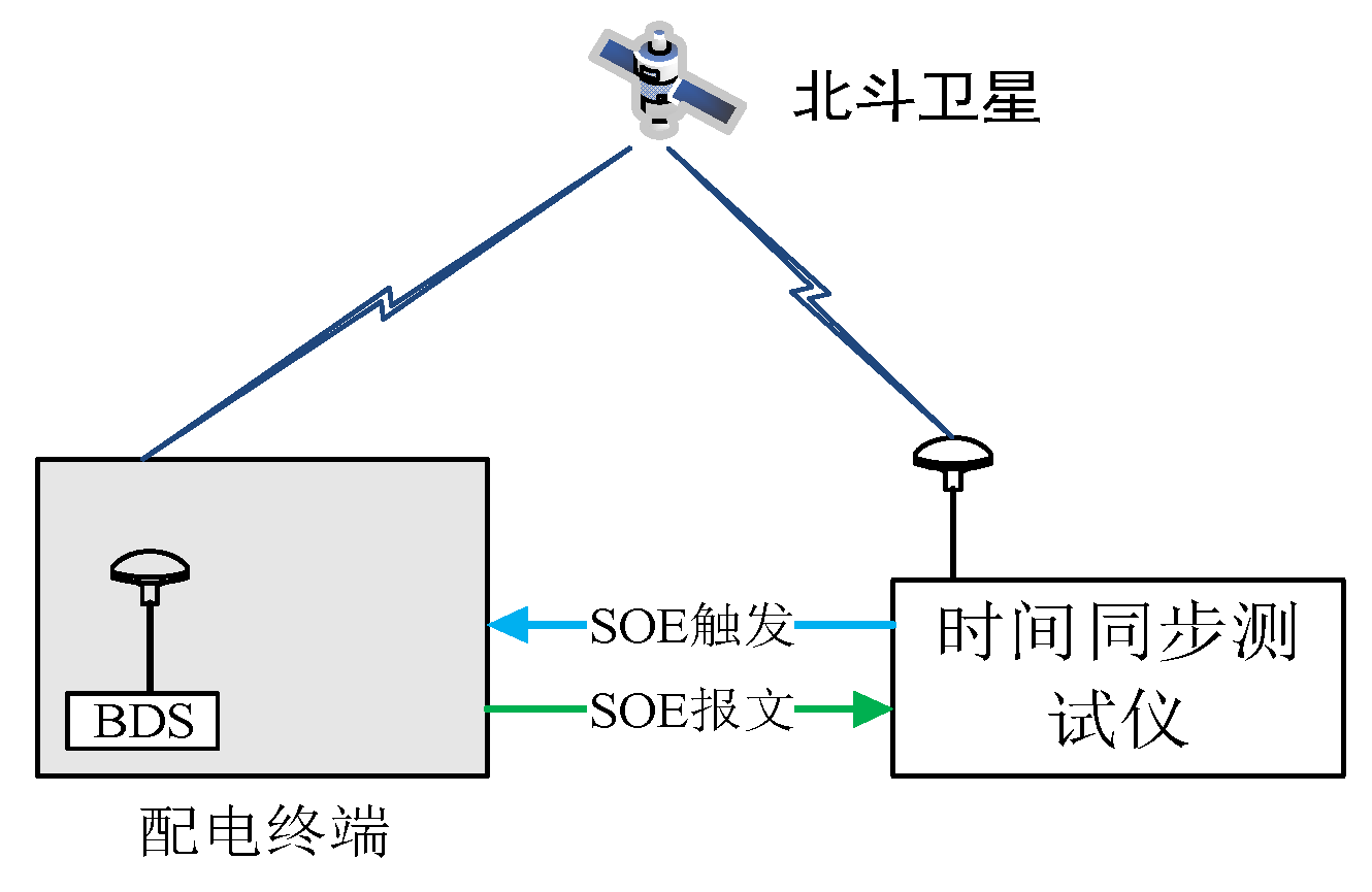
Test method
Distribution terminals A and B received BeiDou satellite signals and synchronized normally for 10 minutes;
Set the timed tripping moment for distribution terminal A and the timed closing moment for distribution terminal B via master station commands;
Tested the contact opening moment of circuit breaker A and the contact closing moment of circuit breaker B using a time synchronization tester;
Compared the time difference between the contact opening moment of circuit breaker A and the contact closing moment of circuit breaker B;
Repeat the test 10 times.
Experimental data

Table 8.
Accuracy test data for timed action of distribution terminals.
| NO. | The moment when Circuit Breaker A opens | Closing time of Circuit Breaker B | Time difference (ms) |
|---|---|---|---|
| 1 | 18:56:20.241 | 18:56:20.249 | 8 |
| 2 | 18:59:50.839 | 18:59:50.849 | 10 |
| 3 | 20:03:10.441 | 20:03:10.443 | 2 |
| 4 | 20:05:11.544 | 20:05:11.547 | 3 |
| 5 | 20:11:11.241 | 20:11:11.253 | 12 |
| 6 | 20:14:00.242 | 20:14:00.247 | 5 |
| 7 | 20:17:50.841 | 20:17:50.845 | 4 |
| 8 | 20:18:50.154 | 20:18:50.157 | 3 |
| 9 | 20:23:46.693 | 20:23:46.698 | 5 |
| 10 | 20:35:24.471 | 20:35:24.476 | 5 |
Experimental conclusions
This paper validates the non-exact probability-based synchronous control method through 10 repeated experiments. Experimental results demonstrate that all time differences for disconnection and reconnection operations are controlled within the range of 2–12 ms, fully meeting the 20 ms engineering requirement and effectively avoiding circulating current risks.
The IDM-NCC fusion model employed in this study provides a more reliable time reference for synchronous control by outputting probability intervals for switching action times. Experimental data demonstrate that this model delivers highly credible action time references for control decisions. The “similarity set” output mechanism of the Naive Credal Classifier exhibits strong fault tolerance, effectively mitigating misjudgment risks in complex distribution environments. No control failures due to model misjudgment occurred during experiments, validating the mechanism's practicality. The imprecise probabilistic model and dynamic delay strategy form an effective closed-loop system. The control setting of the dynamic delay time Δt fully utilizes the probability interval information to achieve adaptive tuning, thereby enabling millisecond-level precision control.
This study empirically demonstrates the application value of imprecise probabilistic theory in distribution network control. It significantly enhances the decision-making robustness of the system under small-sample, high-uncertainty conditions, providing a new technical pathway for constructing highly reliable distribution networks.
7. Conclusions
The core contribution of this study lies in establishing an interval predictive control framework that integrates the Imprecise Dirichlet Model (IDM) with the Naive Credal Classifier (NCC). This framework successfully addresses the challenge of prior dependency in predicting switching operation times for distribution networks under small-sample conditions. Compared to traditional Bayesian control methods, this framework maintains the accuracy of uniqueness judgments while effectively identifying and mitigating misclassification risks in uncertain scenarios by outputting ‘similarity sets’.
Simulation and experimental results demonstrate that the proposed method outperforms traditional Bayesian classifier controllers in both temporal prediction accuracy and model robustness, particularly maintaining high classification accuracy under highly uncertain operational conditions. This research provides a novel theoretical framework and practical technical pathway for load synchronous transfer control in distribution networks, offering valuable insights for enhancing grid operational control capabilities under high renewable energy penetration.
Author Contributions
Conceptualization, H.Z. and C.L.; methodology, C.L.; validation, H.Z. C.L. and W.L.; formal analysis, X.S.; investigation, Y.G.; resources, Y.G.; data curation, C.L.; writing—original draft, W.L. and C.L.; writing—review and editing, X.S.; visualization, Y.G.; supervision, H.Z.; project administration, H.Z.; funding acquisition, H.Z. All authors have read and agreed to the published version of the manuscript.
Funding
This research was funded by the project of State Grid Sichuan Electric Power Company Limited,, grant number 52199723001R.
Data Availability Statement
Data are contained within the article.
Acknowledgments
We are grateful to the reviewers for their comprehensive review of this manuscript, as well as for their insightful comments and valuable suggestions that have significantly contributed to enhancing the quality of our work.
Conflicts of Interest
The authors declare no conflicts of interest.
Abbreviations
The following abbreviations are used in this manuscript:
| IDM | Imprecise Dirichlet model |
| NCC | Naive credal classifier |
| DG | Distributed generation |
References
- Zhao, B.; Zhang, X.; Li, Y.; Wang, Z. A novel approach to transformer fault diagnosis using IDM and naive credal classifier. International Journal of Electrical Power & Energy Systems 2019, 105, 846–855. [Google Scholar] [CrossRef]
- Bernard, J.-M. An introduction to the imprecise Dirichlet model for multinomial data. International Journal of Approximate Reasoning 2005, 39, 123–150. [Google Scholar] [CrossRef]
- Yang, G.; Liu, Y.; Liu, Y. System reliability assessment with imprecise probabilities. Applied Sciences 2019, 9, 5422. [Google Scholar] [CrossRef]
- Corani, G.; Zaffalon, M. Learning reliable classifiers from small or incomplete data sets: The naive credal classifier 2. Journal of Biomedical Informatics 2008, 41, 635–643. [Google Scholar] [CrossRef]
- Walley, P. (1991). Statistical reasoning with imprecise probabilities. Chapman & Hall. [CrossRef]
- Abellán, J.; Masegosa, A. Imprecise Dirichlet model for learning multinomial distributions with missing data. International Journal of Approximate Reasoning 2012, 53, 560–577. [Google Scholar] [CrossRef]
- Zaffalon, M.; Corani, G. Robust inference of trees for missing data. Proceedings of the 12th International Conference on Artificial Intelligence and Statistics (AISTATS) 2009, 5, 501–508. [Google Scholar] [CrossRef]
- Corani, G.; Zaffalon, M.; Gabaglio, S. (2011). Learning reliable classifiers from small and incomplete data sets: the naive credal classifier 3. Proceedings of the 11th European Conference on Symbolic and Quantitative Approaches to Reasoning with Uncertainty (ECSQARU), 591-602. [CrossRef]
- Cozman, F.G. Credal networks. Artificial Intelligence 2000, 120, 199–233. [Google Scholar] [CrossRef]
- Masegosa, A. M.; Moral, S. Imprecise probability models for learning multinomial distributions from data. Applications to learning credal networks. International Journal of Approximate Reasoning 2014, 55, 1548–1569. [Google Scholar] [CrossRef]
- Masegosa, A. M.; Moral, S.; Salmerón, A. Learning mixtures of truncated basis functions from data with missing values. International Journal of Approximate Reasoning 2017, 92, 94–111. [Google Scholar] [CrossRef]
- Troffaes, M.C. M.; Coolen, F. P. A. Applying the imprecise Dirichlet model in cases with missing data. Journal of Risk and Reliability 2009, 223, 301–309. [Google Scholar] [CrossRef]
- Walley, P. Inferences from multinomial data: Learning about a bag of marbles. Journal of the Royal Statistical Society: Series B (Methodological) 1996, 58, 3–57. [Google Scholar] [CrossRef]
- Utkin, L. V.; Kozine, I. O. On the imprecise reliability of multi-state systems. Reliability Engineering & System Safety 2010, 95, 68–76. [Google Scholar] [CrossRef]
- Miranda, E.; Zaffalon, M.; de Cooman, G. Conglomerable natural extension. International Journal of Approximate Reasoning 2012, 53, 1200–1227. [Google Scholar] [CrossRef]
- Antucci, A.; Patit, A.; Zaffalon, M. (2007). Credal networks for operational risk measurement and management. In Knowledge-Based Intelligent Information and Engineering Systems (pp. 604–611). Springer. [CrossRef]
- Abellán, J. Uncertainty measures on probability intervals from the imprecise Dirichlet model. International Journal of General Systems 2006, 35, 509–528. [Google Scholar] [CrossRef]
- de, Campos, C. P.; Cozman, F. G. Computing lower and upper expectations under epistemic independence for credal networks. International Journal of Approximate Reasoning 2007, 44, 244–260. [CrossRef]
- Antón, S.; de la Ossa, L. Credal-network based probabilistic argumentation with incomplete evidence. International Journal of Approximate Reasoning 2022, 146, 1–20. [Google Scholar] [CrossRef]
- Sistani, A.; Hosseini, S. A.; Sadeghi, V. S.; Taheri, B. Fault detection in a single-bus DC microgrid connected to EV/PV systems and hybrid energy storage using the DMD-IF method. Sustainability 2023, 15, 16269. [Google Scholar] [CrossRef]
- de Cooman, G.; De Bock, J.; Diniz, M. A. Predictive inference under exchangeability and the Imprecise Dirichlet Multinomial Model. International Journal of Approximate Reasoning 2021, 138, 1–26. [Google Scholar] [CrossRef]
Figure 1.
A simple diagram of the principle of Bayes classifier.
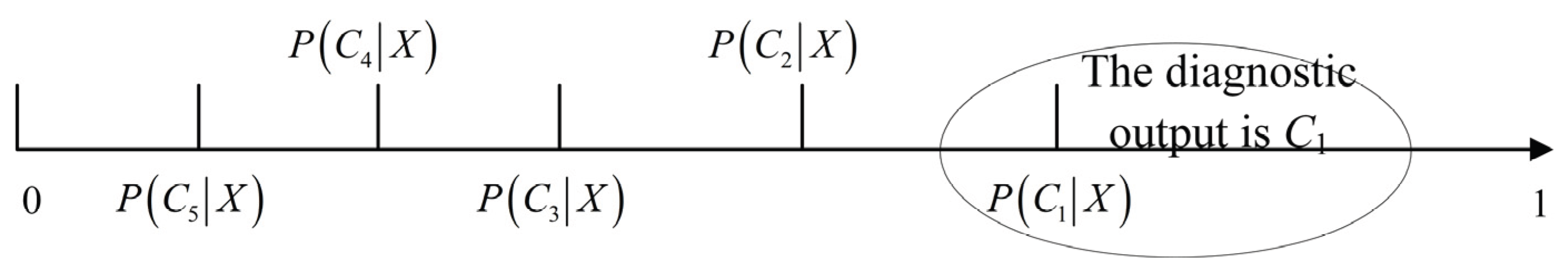
Figure 2.
The credal network output is a unique class case.
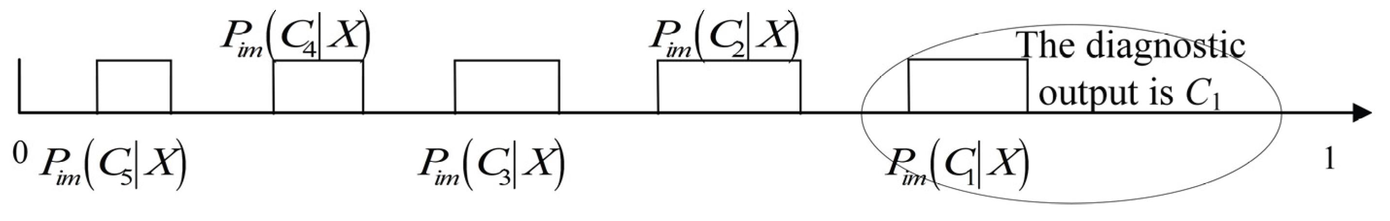
Figure 3.
The credal network output is a similar class set case.
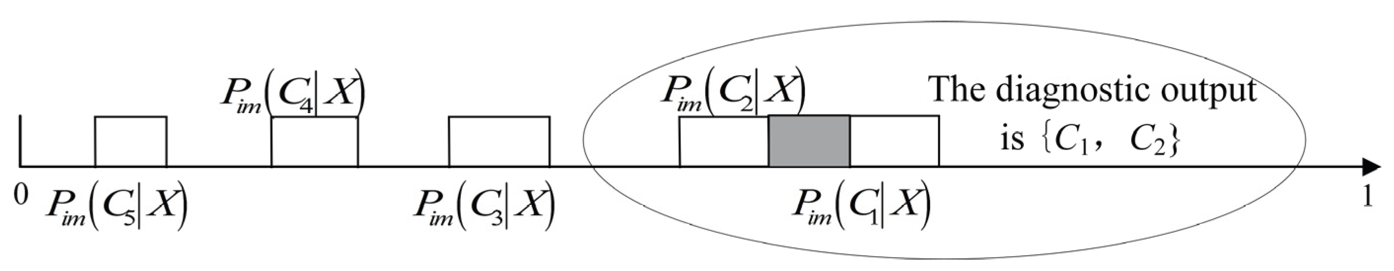
Figure 4.
Distribution network switch action time prediction credal network splitter diagram.
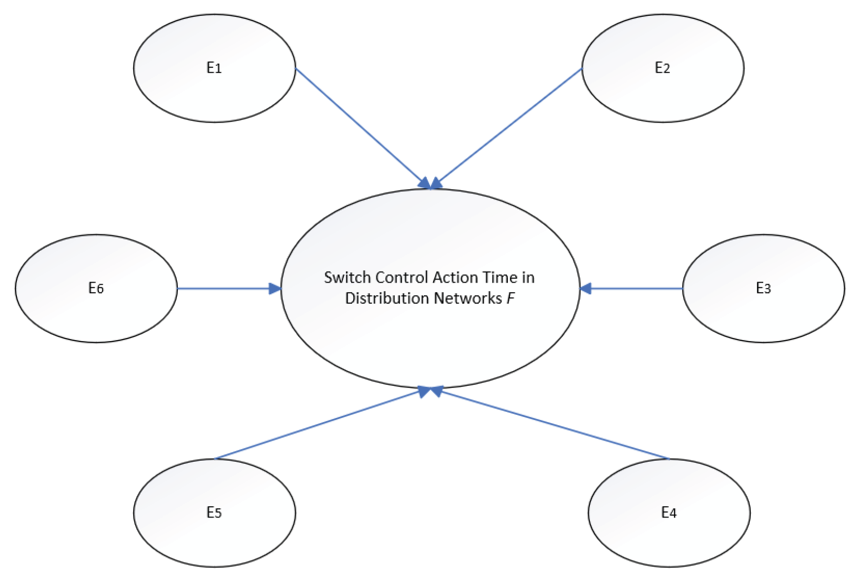
Figure 5.
Flow chart of switching action time of distribution network based on imprecise probability.
Figure 5.
Flow chart of switching action time of distribution network based on imprecise probability.
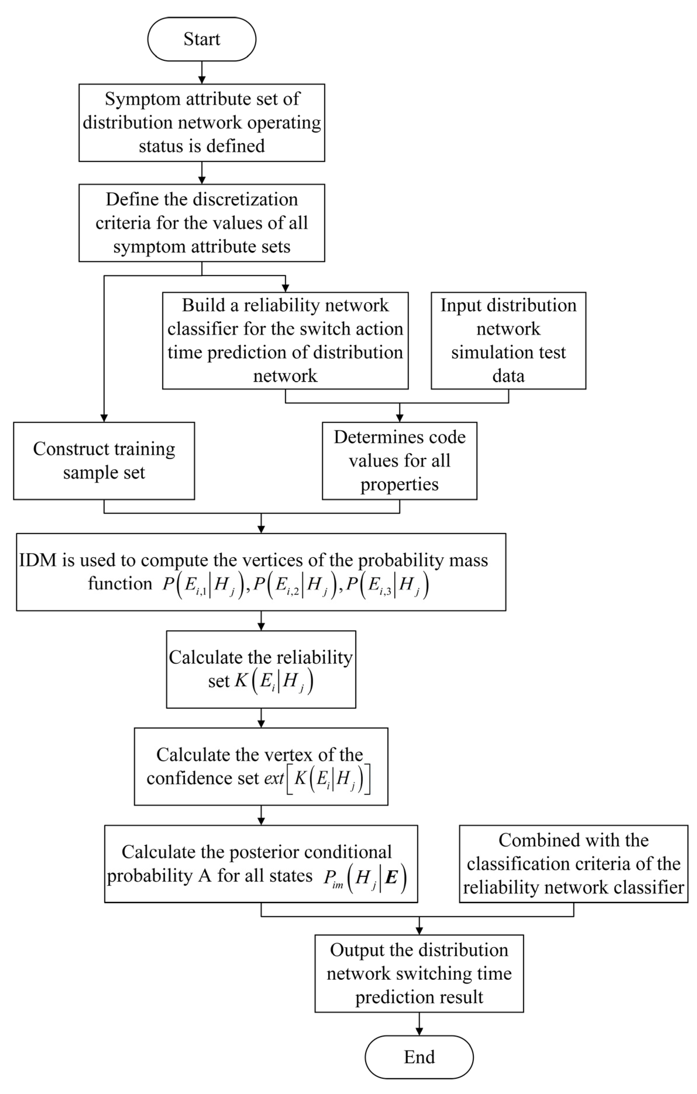
Table 1.
Distribution network switching time status class.
| No. | Switch control action time T/ms | No. | Switch control action time T/ms |
|---|---|---|---|
| F1 | T<5 | F18 | 26≤T<27 |
| F2 | 5≤T<10 | F19 | 27≤T<28 |
| F3 | 10≤T<11 | F20 | 28≤T<29 |
| F4 | 11≤T<12 | F21 | 29≤T<30 |
| F5 | 12≤T<13 | F22 | 30≤T<31 |
| F6 | 13≤T<14 | F23 | 31≤T<32 |
| F7 | 14≤T<15 | F24 | 32≤T<33 |
| F8 | 15≤T<16 | F25 | 33≤T<34 |
| F9 | 16≤T<17 | F26 | 34≤T<35 |
| F10 | 17≤T<18 | F27 | 35≤T<36 |
| F11 | 18≤T<19 | F28 | 36≤T<37 |
| F12 | 20≤T<21 | F29 | 37≤T<38 |
| F13 | 21≤T<22 | F30 | 38≤T<39 |
| F14 | 22≤T<23 | F31 | 39≤T<40 |
| F15 | 23≤T<24 | F32 | 40≤T<50 |
| F16 | 24≤T<25 | F33 | 50≤T<60 |
| F17 | 25≤T<26 | F34 | T≥60 |
Table 2.
Distribution network action state symptom attribute set.
| Variables | Sign type |
|---|---|
| E1 | Peak of phase A voltage |
| E2 | Peak of phase B voltage |
| E3 | Peak of phase C voltage |
| E4 | Peak of phase A current |
| E5 | Peak of phase B current |
| E6 | Peak of phase C current |
Table 3.
Normalized database of eigenmatrix.
| E1 | E2 | E3 | E4 | E5 | E6 | |
|---|---|---|---|---|---|---|
| S1 | 0.6317 | 0.9733 | 0.9689 | -0.9922 | -0.9921 | -0.9922 |
| S2 | -0.1786 | 0.9688 | 0.9778 | -0.0907 | -0.9890 | -0.9905 |
| S3 | 0.6390 | -0.0111 | 0.9689 | -0.9913 | -0.0893 | -0.9898 |
| S4 | 0.6317 | 0.9777 | -0.0044 | -0.9898 | -0.9912 | -0.0893 |
| S5 | -0.6317 | -0.3541 | 0.9822 | 0.7220 | 0.6905 | -0.9921 |
| ⁝ | ⁝ | ⁝ | ⁝ | ⁝ | ⁝ | ⁝ |
| S310 | 0.3076 | 0.5724 | 0.5733 | -0.5693 | -0.5682 | -0.5682 |
Table 4.
Calculation results of switch control time state class of distribution network based on imprecise probability.
Table 4.
Calculation results of switch control time state class of distribution network based on imprecise probability.
| Imprecise probability | Probability value | Imprecise probability | Probability value |
|---|---|---|---|
| Pim(F1│S1) | [1.60×10⁻⁵, 5.57×10⁻⁵] | Pim(F18│S1) | [3.69×10⁻¹¹, 1.50×10⁻¹⁰] |
| Pim(F2│S1) | [5.78×10⁻⁶, 7.34×10⁻⁶] | Pim(F19│S1) | [5.22×10⁻¹², 1.24×10⁻¹⁰] |
| Pim(F3│S1) | [3.00×10⁻⁶, 7.34×10⁻⁶] | Pim(F20│S1) | [1.43×10⁻¹⁰, 4.36×10⁻¹⁰] |
| Pim(F4│S1) | [1.54×10⁻⁶, 1.74×10⁻⁶] | Pim(F21│S1) | [9.89×10⁻¹¹, 1.04×10⁻¹⁰] |
| Pim(F5│S1) | [5.36×10⁻⁷, 5.70×10⁻⁷] | Pim(F22│S1) | [6.53×10⁻¹¹, 7.34×10⁻¹¹] |
| Pim(F6│S1) | [1.04×10⁻⁸, 2.29×10⁻⁷] | Pim(F23│S1) | [4.31×10⁻¹¹, 6.23×10⁻¹¹] |
| Pim(F7│S1) | [3.87×10⁻⁶, 7.34×10⁻⁶] | Pim(F24│S1) | [1.11×10⁻¹¹, 1.74×10⁻¹¹] |
| Pim(F8│S1) | [6.63×10⁻⁷, 7.42×10⁻⁷] | Pim(F25│S1) | [5.28×10⁻¹¹, 5.31×10⁻¹¹] |
| Pim(F9│S1) | [2.65×10⁻⁹, 4.80×10⁻⁹] | Pim(F26│S1) | [2.99×10⁻¹¹, 4.55×10⁻¹¹] |
| Pim(F10│S1) | [8.14×10⁻⁹, 1.78×10⁻⁸] | Pim(F27│S1) | [1.06×10⁻¹⁰, 1.50×10⁻¹⁰] |
| Pim(F11│S1) | [6.89×10⁻¹⁰, 7.20×10⁻¹⁰] | Pim(F28│S1) | [2.37×10⁻¹⁰, 4.36×10⁻¹⁰] |
| Pim(F12│S1) | [1.98×10⁻¹⁰, 4.36×10⁻¹⁰] | Pim(F29│S1) | [2.06×10⁻¹⁰, 3.46×10⁻¹⁰] |
| Pim(F13│S1) | [0, 7.20×10⁻¹⁰] | Pim(F30│S1) | [1.24×10⁻², 4.28×10⁻²] |
| Pim(F14│S1) | [8.51×10⁻¹⁰, 1.26×10⁻⁹] | Pim(F31│S1) | [1.85×10⁻¹⁰, 1.26×10⁻⁹] |
| Pim(F15│S1) | [3.19×10⁻¹⁰, 5.57×10⁻¹⁰] | Pim(F32│S1) | [2.91×10⁻⁸, 3.02×10⁻⁸] |
| Pim(F16│S1) | [2.85×10⁻¹¹, 2.77×10⁻¹⁰] | Pim(F33│S1) | [2.07×10⁻⁷, 2.29×10⁻⁷] |
| Pim(F17│S1) | [3.93×10⁻¹⁰, 4.36×10⁻¹⁰] | Pim(F34│S1) | [3.94×10⁻⁷, 5.70×10⁻⁷] |
Table 5.
Calculation results of switch control time state class of distribution network based on precise single value probability.
Table 5.
Calculation results of switch control time state class of distribution network based on precise single value probability.
| Exact probability | Probability value | Exact probability | Probability value |
|---|---|---|---|
| P(F1│S1) | 2.74×10⁻⁵ | P(F18│S1) | 6.48×10⁻¹¹ |
| P(F2│S1) | 7.01×10⁻⁶ | P(F19│S1) | 1.02×10⁻¹¹ |
| P(F3│S1) | 4.77×10⁻⁶ | P(F20│S1) | 2.39×10⁻¹⁰ |
| P(F4│S1) | 1.72×10⁻⁶ | P(F21│S1) | 1.03×10⁻¹⁰ |
| P(F5│S1) | 5.68×10⁻⁷ | P(F22│S1) | 7.25×10⁻¹¹ |
| P(F6│S1) | 2.04×10⁻⁸ | P(F23│S1) | 5.64×10⁻¹¹ |
| P(F7│S1) | 5.70×10⁻⁶ | P(F24│S1) | 1.52×10⁻¹¹ |
| P(F8│S1) | 7.34×10⁻⁷ | P(F25│S1) | 5.31×10⁻¹¹ |
| P(F9│S1) | 3.83×10⁻⁹ | P(F26│S1) | 4.01×10⁻¹¹ |
| P(F10│S1) | 1.26×10⁻⁸ | P(F27│S1) | 1.37×10⁻¹⁰ |
| P(F11│S1) | 7.19×10⁻¹⁰ | P(F28│S1) | 3.46×10⁻¹⁰ |
| P(F12│S1) | 3.06×10⁻¹⁰ | P(F29│S1) | 2.89×10⁻¹⁰ |
| P(F13│S1) | 0 | P(F30│S1) | 2.12×10⁻² |
| P(F14│S1) | 1.12×10⁻⁹ | P(F31│S1) | 3.42×10⁻¹⁰ |
| P(F15│S1) | 4.55×10⁻¹⁰ | P(F32│S1) | 3.01×10⁻⁸ |
| P(F16│S1) | 5.41×10⁻¹¹ | P(F33│S1) | 2.27×10⁻⁷ |
| P(F17│S1) | 4.32×10⁻¹⁰ | P(F34│S1) | 5.16×10⁻⁷ |
Table 6.
Calculation results of switching time state class of distribution network based on imprecise probability.
Table 6.
Calculation results of switching time state class of distribution network based on imprecise probability.
| Imprecise probability | Probability value | Imprecise probability | Probability value |
|---|---|---|---|
| Pim(F1│S1) | [1.60×10⁻⁵, 5.57×10⁻⁵] | Pim(F18│S1) | [6.31×10⁻¹², 1.50×10⁻¹⁰] |
| Pim(F2│S1) | [5.78×10⁻⁶, 7.34×10⁻⁶] | Pim(F19│S1) | [4.07×10⁻¹¹, 1.24×10⁻¹⁰] |
| Pim(F3│S1) | [3.00×10⁻⁶, 7.34×10⁻⁶] | Pim(F20│S1) | [4.17×10⁻¹⁰, 4.36×10⁻¹⁰] |
| Pim(F4│S1) | [1.54×10⁻⁶, 1.74×10⁻⁶] | Pim(F21│S1) | [9.21×10⁻¹¹, 1.04×10⁻¹⁰] |
| Pim(F5│S1) | [5.36×10⁻⁷, 5.70×10⁻⁷] | Pim(F22│S1) | [3.70×10⁻², 5.35×10⁻²] |
| Pim(F6│S1) | [1.04×10⁻⁸, 2.29×10⁻⁷] | Pim(F23│S1) | [3.54×10⁻², 5.53×10⁻²] |
| Pim(F7│S1) | [3.87×10⁻⁶, 7.34×10⁻⁶] | Pim(F24│S1) | [1.73×10⁻¹¹, 1.74×10⁻¹¹] |
| Pim(F8│S1) | [9.46×10⁻⁸, 1.06×10⁻⁷] | Pim(F25│S1) | [3.48×10⁻¹¹, 5.31×10⁻¹¹] |
| Pim(F9│S1) | [2.65×10⁻⁹, 4.80×10⁻⁹] | Pim(F26│S1) | [3.23×10⁻¹¹, 4.55×10⁻¹¹] |
| Pim(F10│S1) | [8.14×10⁻⁹, 1.78×10⁻⁸] | Pim(F27│S1) | [8.16×10⁻¹¹, 1.50×10⁻¹⁰] |
| Pim(F11│S1) | [6.89×10⁻¹⁰, 7.20×10⁻¹⁰] | Pim(F28│S1) | [2.59×10⁻¹⁰, 4.36×10⁻¹⁰] |
| Pim(F12│S1) | [1.98×10⁻¹⁰, 4.36×10⁻¹⁰] | Pim(F29│S1) | [1.00×10⁻¹⁰, 3.46×10⁻¹⁰] |
| Pim(F13│S1) | [4.88×10⁻¹⁰, 7.20×10⁻¹⁰] | Pim(F30│S1) | [3.29×10⁻¹¹, 2.24×10⁻¹⁰] |
| Pim(F14│S1) | [7.19×10⁻¹⁰, 1.26×10⁻⁹] | Pim(F31│S1) | [1.21×10⁻⁹, 1.26×10⁻⁹] |
| Pim(F15│S1) | [5.73×10⁻¹¹, 5.57×10⁻¹⁰] | Pim(F32│S1) | [2.72×10⁻⁸, 3.02×10⁻⁸] |
| Pim(F16│S1) | [2.49×10⁻¹⁰, 2.77×10⁻¹⁰] | Pim(F33│S1) | [0, 2.29×10⁻⁷] |
| Pim(F17│S1) | [1.07×10⁻¹⁰, 4.36×10⁻¹⁰] | Pim(F34│S1) | [0, 5.70×10⁻⁷] |
Table 7.
Calculation results of switching time state class of distribution network based on precise single value probability.
Table 7.
Calculation results of switching time state class of distribution network based on precise single value probability.
| Exact probability | Probability value | Exact probability | Probability value |
|---|---|---|---|
| P(F1│S1) | 2.74×10⁻⁵ | P(F18│S1) | 1.24×10⁻¹¹ |
| P(F2│S1) | 7.01×10⁻⁶ | P(F19│S1) | 6.81×10⁻¹¹ |
| P(F3│S1) | 4.77×10⁻⁶ | P(F20│S1) | 4.36×10⁻¹⁰ |
| P(F4│S1) | 1.72×10⁻⁶ | P(F21│S1) | 1.02×10⁻¹⁰ |
| P(F5│S1) | 5.68×10⁻⁷ | P(F22│S1) | 5.18×10⁻² |
| P(F6│S1) | 2.04×10⁻⁸ | P(F23│S1) | 5.36×10⁻² |
| P(F7│S1) | 5.70×10⁻⁶ | P(F24│S1) | 1.74×10⁻¹¹ |
| P(F8│S1) | 1.05×10⁻⁷ | P(F25│S1) | 4.65×10⁻¹¹ |
| P(F9│S1) | 3.83×10⁻⁹ | P(F26│S1) | 4.55×10⁻¹¹ |
| P(F10│S1) | 1.26×10⁻⁸ | P(F27│S1) | 1.26×10⁻¹⁰ |
| P(F11│S1) | 7.19×10⁻¹⁰ | P(F28│S1) | 3.85×10⁻¹⁰ |
| P(F12│S1) | 3.06×10⁻¹⁰ | P(F29│S1) | 2.34×10⁻¹⁰ |
| P(F13│S1) | 6.45×10⁻¹⁰ | P(F30│S1) | 1.46×10⁻¹⁰ |
| P(F14│S1) | 1.03×10⁻⁹ | P(F31│S1) | 1.22×10⁻⁹ |
| P(F15│S1) | 1.09×10⁻¹⁰ | P(F32│S1) | 2.77×10⁻⁸ |
| P(F16│S1) | 2.74×10⁻¹⁰ | P(F33│S1) | 2.21×10⁻⁷ |
| P(F17│S1) | 1.88×10⁻¹⁰ | P(F34│S1) | 5.15×10⁻⁷ |
Disclaimer/Publisher’s Note: The statements, opinions and data contained in all publications are solely those of the individual author(s) and contributor(s) and not of MDPI and/or the editor(s). MDPI and/or the editor(s) disclaim responsibility for any injury to people or property resulting from any ideas, methods, instructions or products referred to in the content. |
© 2025 by the authors. Licensee MDPI, Basel, Switzerland. This article is an open access article distributed under the terms and conditions of the Creative Commons Attribution (CC BY) license (http://creativecommons.org/licenses/by/4.0/).
Copyright: This open access article is published under a Creative Commons CC BY 4.0 license, which permit the free download, distribution, and reuse, provided that the author and preprint are cited in any reuse.


