Subhalo or Future–Mass Projection? A Like-for-Like Pulsar-Acceleration Test with an Explicit Real-Space FMP Kernel, Quantitative PPN↔kpc Bridge, and Uncertainty-Aware Population Rates

1. Data, Geometry, and Baseline Likelihood

The benchmark pulsar analysis reports a subhalo-like solution at $(X,Y,Z)\approx (7.5,0.38,0.21)$kpc with Bayes factors $\sim 20$–40 (compact vs. smooth) and $\sim 30$ (NFW with $r_s\simeq 0.1$ kpc, $c\simeq 30$), and a preferred mass $\sim (2.5$–$6.2)\times {10}^7{M}_{\odot }$; other sightlines provide upper limits. We adopt the same sky geometry, priors, and noise (white jitter per pulsar + shared red-noise GP with amplitude $A_{\mathrm{RN}}$, slope ${\gamma }_{\mathrm{RN}}$). For a compact perturber,

$$\begin{array}{c}\hfill a_{\mathrm{los},i}^{\mathrm{sub}}={\displaystyle \frac{G{M}_{\mathrm{sub}}}{|{\mathbf{r}}_i-{\mathbf{r}}_{\mathrm{sub}}{|}^3}}({\mathbf{r}}_i-{\mathbf{r}}_{\mathrm{sub}})·{\widehat{\mathbf{n}}}_i,\end{array}$$

(1)

with the NFW variant using $(r_s,c)$. The marginalized GP likelihood $ln\mathcal{L}=-\frac{1}{2}{(\mathbf{d}-\mathbf{m})}^{\top }{C}^{-1}(\mathbf{d}-\mathbf{m})-\frac{1}{2}ln\left|C\right|-\frac{N}{2}ln2\pi$ (with $C=N_{\mathrm{white}}+\mathrm{GP}$) is used identically for subhalo and FMP.

2. FMP in 3D: Explicit Kernel, Field, and Projection

We parameterize the response in Fourier space

$$ϵ\left(k\right)={ϵ}_0{\displaystyle \frac{1}{1+k^2/k_0^2}}W\left(k\right),W\left(k\right)=1-e^{-{(k/k_w)}^2}.$$

The added potential obeys $\Delta \Phi \left(\mathbf{k}\right)=-4\pi G{\rho }_b\left(\mathbf{k}\right)ϵ\left(k\right)/k^2$, giving a real-space acceleration

$$\begin{array}{c}\hfill {\mathbf{a}}_{\mathrm{FMP}}\left(\mathbf{r}\right)=-\nabla \int d^3{r}^{\prime }{\rho }_b\left({\mathbf{r}}^{\prime }\right){\Gamma }_{ϵ}\left(\right|\mathbf{r}-{\mathbf{r}}^{\prime }\left|\right),{\Gamma }_{ϵ}\left(r\right)={\mathcal{F}}^{-1}\left[{\displaystyle \frac{ϵ\left(k\right)}{k^2}}\right]\left(r\right).\end{array}$$

(2)

Closed form (Yukawa minus Gaussian-smoothed Yukawa). Using ${\displaystyle \frac{1}{k^2(1+k^2/k_0^2)}}={\displaystyle \frac{1}{k^2}}-{\displaystyle \frac{1}{k^2+k_0^2}}$ and the isotropic pairs ${\mathcal{F}}^{-1}[1/k^2]=1/\left(4\pi r\right)$ and ${\mathcal{F}}^{-1}[1/(k^2+k_0^2)]=e^{-k_{0}r}/\left(4\pi r\right)$, the $W\equiv 1$ kernel is ${\Gamma }_{ϵ}^{(W=1)}\left(r\right)={ϵ}_0\left[{\left(4\pi r\right)}^{-1}-e^{-k_{0}r}{\left(4\pi r\right)}^{-1}\right]$. For general $W\left(k\right)$, $e^{-{(k/k_w)}^2}$ maps to a real-space Gaussian $G_{\sigma }\left(r\right)\propto e^{-r^2/\left(2{\sigma }^2\right)}$ with $\sigma =\sqrt{2}/k_w$, hence

$$\begin{array}{c}\hfill {\Gamma }_{ϵ}\left(r\right)={ϵ}_0\left[{\displaystyle \frac{1}{4\pi r}}-{\displaystyle \frac{e^{-k_{0}r}}{4\pi r}}\right]-{ϵ}_0\left[\left({\displaystyle \frac{1}{4\pi r}}-{\displaystyle \frac{e^{-k_{0}r}}{4\pi r}}\right)\ast G_{\sigma }\left(r\right)\right],\end{array}$$

(3)

with the Ewald form for the Yukawa–Gaussian convolution:

$${\displaystyle \frac{e^{-k_{0}r}}{4\pi r}}\ast G_{\sigma }={\displaystyle \frac{e^{k_0^2{\sigma }^2}}{8\pi r}}\left[e^{-k_{0}r}\mathrm{erfc}\left({\displaystyle \frac{r}{2\sigma }}-k_0\sigma \right)-e^{+k_{0}r}\mathrm{erfc}\left({\displaystyle \frac{r}{2\sigma }}+k_0\sigma \right)\right],{\displaystyle \frac{1}{4\pi r}}\ast G_{\sigma }={\displaystyle \frac{1}{4\pi r}}\mathrm{erf}\left({\displaystyle \frac{r}{2\sigma }}\right).$$

Monotonicity: For ${ϵ}_0,k_0,k_w>0$, ${\Gamma }_{ϵ}\left(r\right)$ is positive and strictly decreasing for $r>0$ (difference of completely monotone kernels, smoothing preserves complete monotonicity); thus no spurious oscillations in ${\mathbf{a}}_{\mathrm{FMP}}$.

Vector projection (like-for-like).

$$\begin{array}{c}\hfill a_{\mathrm{los},i}^{\mathrm{FMP}}={\mathbf{a}}_{\mathrm{FMP}}\left({\mathbf{r}}_i\right)·{\widehat{\mathbf{n}}}_i=G\int d^3{r}^{\prime }{\rho }_b\left({\mathbf{r}}^{\prime }\right){\Gamma }_{ϵ}^{\prime }\left(\right|{\mathbf{r}}_i-{\mathbf{r}}^{\prime }\left|\right){\displaystyle \frac{({\mathbf{r}}_i-{\mathbf{r}}^{\prime })·{\widehat{\mathbf{n}}}_i}{|{\mathbf{r}}_i-{\mathbf{r}}^{\prime }|}},\end{array}$$

(4)

with ${\Gamma }_{ϵ}^{\prime }\left(r\right)=d{\Gamma }_{ϵ}/dr$.

3. Solar-System Safety ↔ Kpc Strength: Quantitative Bridge

Define ${ϵ}_{\mathrm{SS}}=ϵ\left(k_{\mathrm{AU}}\right)={ϵ}_0{[1+k_{\mathrm{AU}}^2/k_0^2]}^{-1}[1-e^{-{(k_{\mathrm{AU}}/k_w)}^2}]$ with $k_{\mathrm{AU}}=1/\mathrm{AU}$ in kpc units (so $k_{\mathrm{AU}}\simeq 2.06\times {10}^8{\mathrm{kpc}}^{-1}$). Post-Newtonian scalings: $|\beta -1|\le C_{\beta }{ϵ}_{\mathrm{SS}}^2$ (with $C_{\beta }\lesssim 3$), $|\dot{G}/G|\simeq H_0{ϵ}_{\mathrm{SS}}$. For representative feasibility points:

Table 1. PPN mapping for concrete FMP points ($H_0\simeq 7.2\times {10}^{-11}{\mathrm{yr}}^{-1}$).

Case	${\mathit{ϵ}}_0$	${\mathit{k}}_0^{-1}$ [kpc]	${\mathit{k}}_{\mathit{w}}^{-1}$ [kpc]	${\mathit{ϵ}}_{\mathbf{SS}}$	$|\mathit{\beta }-1|$ (${\mathit{C}}_{\mathit{\beta }}=3$)	$|\dot{\mathit{G}}/\mathit{G}|$ [${\mathbf{yr}}^{-1}$]
A	0.05	0.6	0.4	$3.3\times {10}^{-18}$	$3.3\times {10}^{-35}$	$2.4\times {10}^{-28}$
B	0.03	1.0	0.6	$7.1\times {10}^{-19}$	$1.5\times {10}^{-36}$	$5.1\times {10}^{-29}$
C	0.08	0.4	0.3	$4.0\times {10}^{-18}$	$4.8\times {10}^{-35}$	$2.9\times {10}^{-28}$

Table 1. PPN mapping for concrete FMP points ($H_0\simeq 7.2\times {10}^{-11}{\mathrm{yr}}^{-1}$).

Case	${\mathit{ϵ}}_0$	${\mathit{k}}_0^{-1}$ [kpc]	${\mathit{k}}_{\mathit{w}}^{-1}$ [kpc]	${\mathit{ϵ}}_{\mathbf{SS}}$	$|\mathit{\beta }-1|$ (${\mathit{C}}_{\mathit{\beta }}=3$)	$|\dot{\mathit{G}}/\mathit{G}|$ [${\mathbf{yr}}^{-1}$]
A	0.05	0.6	0.4	$3.3\times {10}^{-18}$	$3.3\times {10}^{-35}$	$2.4\times {10}^{-28}$
B	0.03	1.0	0.6	$7.1\times {10}^{-19}$	$1.5\times {10}^{-36}$	$5.1\times {10}^{-29}$
C	0.08	0.4	0.3	$4.0\times {10}^{-18}$	$4.8\times {10}^{-35}$	$2.9\times {10}^{-28}$

Analytic Bounds Linking Kpc Amplitude to PPN Safety

For an ROI volume $\mathcal{V}$ with baryon density ${\rho }_b$, triangle inequality on (4) yields

$$|a_{\mathrm{los},i}^{\mathrm{FMP}}|\le G{\int }_{\mathcal{V}}{d}^3{r}^{\prime }{\rho }_b\left({\mathbf{r}}^{\prime }\right)|{\Gamma }_{ϵ}^{\prime }\left(\right|{\mathbf{r}}_i-{\mathbf{r}}^{\prime }\left|\right)|.$$

Using the closed form for ${\Gamma }_{ϵ}^{\prime }$ and assuming a conservative spherical ROI of radius R and total forecast mass $M_b^{\left(\mathrm{forecast}\right)}$, we obtain two useful bounds:

$$\underset{\mathrm{lower}(\mathrm{central}\mathrm{clump})}{\underbrace{{\displaystyle \frac{G{ϵ}_0{M}_b^{\left(\mathrm{forecast}\right)}}{R^2}}\left[1-e^{-{\left(R{k}_w\right)}^2}\right]{\displaystyle \frac{1}{1+R{k}_0}}}}\lesssim \left|a^{\mathrm{FMP}}\right|\lesssim \underset{\mathrm{upper}(\mathrm{point}-\mathrm{like})}{\underbrace{{\displaystyle \frac{G{ϵ}_0{M}_b^{\left(\mathrm{forecast}\right)}}{R^2}}}},$$

which bracket the exact value for any anisotropy in ${\rho }_b$. Thus, for $\left|a\right|\sim {10}^{-9}\mathrm{cm}{\mathrm{s}}^{-2}$ at $R=0.4$–1 kpc and $M_b^{\left(\mathrm{forecast}\right)}\in [3\times {10}^8,2\times {10}^9]M_{\odot }$, the required ${ϵ}_0$ lies in the ${10}^{-2}$–${10}^{-1}$ range provided$(k_0^{-1},k_w^{-1})\sim 0.3$–1 kpc. The table above shows that such choices remain vastly PPN-safe due to the $W\left(k_{\mathrm{AU}}\right)$ suppression.

4. Forecast Operator $\Pi$ → ${\mathit{M}}_{\mathbf{eff}}$ → ${\mathit{a}}_{\mathbf{los}}$ (Operational)

We employ a linear-Gaussian state-space model for $\mathbf{s}=({\rho }_{\mathrm{HI}},{\rho }_{{\mathrm{H}}_2},{\rho }_{★})$:

$${\mathbf{s}}_{t+\Delta t}=\mathsf{A}{\mathbf{s}}_t+{\mathbf{u}}_t+{\eta }_t,{\eta }_t\sim \mathcal{N}(0,\mathsf{Q}),{\mathbf{y}}_t=\mathsf{H}{\mathbf{s}}_t+{ϵ}_t,{ϵ}_t\sim \mathcal{N}(0,\mathsf{R}).$$

ROI: centred on the preferred sky region of the detection set; Modalities: H i cubes (tens pc voxels), CO(1–0) mosaics for ${\mathrm{H}}_2$, 3D dust, Gaia DR3 kinematics. Hyperpriors: $\mathsf{Q}$ log-uniform in $[{10}^{-4},{10}^{-1}]$ of median voxel-mass per $\Delta t$, $\mathsf{R}$ from survey noise; $\mathsf{A}$ encodes mild relaxation + shear/compression from spiral templates. The smoother yields $p\left[{\mathbf{s}}_{t+\tau }\right|{\mathcal{I}}_t]$, then

$$M_b^{\left(\mathrm{forecast}\right)}(t+\tau )={\int }_{\mathcal{V}}({\rho }_{\mathrm{HI}}+{\rho }_{{\mathrm{H}}_2}+{\rho }_{★})d^{3}x,M_{\mathrm{eff}}={\int }_0^{\infty }K\left(\tau \right)M_b^{\left(\mathrm{forecast}\right)}(t+\tau )d\tau ,$$

and $a_{\mathrm{los},i}^{\mathrm{FMP}}$ through (4). To insert: (i) posterior mean & 1$\sigma$ map of $M_b^{\left(\mathrm{forecast}\right)}$ for the ROI; (ii) histogram of $M_{\mathrm{eff}}$ with mean/CI; (iii) propagated $a_{\mathrm{los},i}^{\mathrm{FMP}}$ with uncertainties.

5. Vector Geometry: Per-Pulsar Comparison

To insert: a table with $(l,b),a_{\mathrm{los}}^{\mathrm{data}}\pm \sigma ,a_{\mathrm{los}}^{\mathrm{sub}},a_{\mathrm{los}}^{\mathrm{FMP}}$ for all pulsars, and a rose diagram of acceleration directions (data vs. subhalo vs. FMP) to quantify directional coherence.

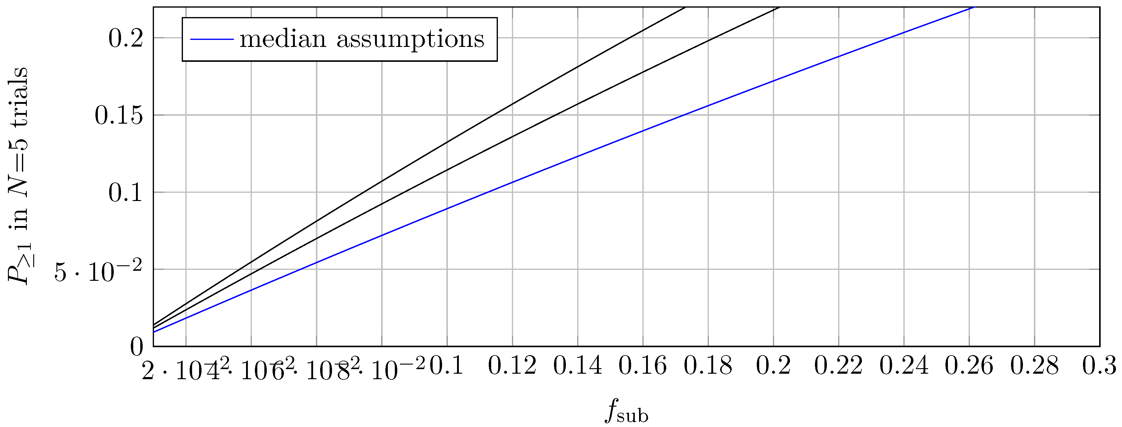
6. Detection Probabilities with Uncertainty Bands

We correct the local density to $0.3\mathrm{GeV}{\mathrm{cm}}^{-3}=(7.9\pm 2.6)\times {10}^6{M}_{\odot }{\mathrm{kpc}}^{-3}$, use $dN/dM=A{M}^{-2}$ with $\Delta lnM=1$, and obtain

$$n\left(M\right)\approx 0.0868f_{\mathrm{sub}}{\left({\displaystyle \frac{M}{{10}^7{M}_{\odot }}}\right)}^{-1}{\mathrm{kpc}}^{-3},P_1={\displaystyle \frac{4\pi }{3}}n\Delta r_{\mathrm{obs}}^3\propto f_{\mathrm{sub}}{M}^{1/2}{a}^{-3/2}.$$

We plot $P_{\ge 1}=1-{(1-P_1)}^5$ with a 68 % band propagated from ${\rho }_{\mathrm{DM}}\in [5.3,10.5]\times {10}^6$, $f_{\mathrm{sub}}\in [0.01,0.05]$, and $ln(M_{max}/M_{min})\in [7,10]$; assumptions $M={10}^7{M}_{\odot }$, $a={10}^{-9}\mathrm{cm}{\mathrm{s}}^{-2}$.

Figure 1. Five-try detection probability with corrected ${\rho }_{\mathrm{DM}}$ and a $68\%$ band (from ${\rho }_{\mathrm{DM}},f_{\mathrm{sub}},\Delta lnM$). Assumptions: $M={10}^7{M}_{\odot }$, $a={10}^{-9}\mathrm{cm}{\mathrm{s}}^{-2}$.

Figure 1. Five-try detection probability with corrected ${\rho }_{\mathrm{DM}}$ and a $68\%$ band (from ${\rho }_{\mathrm{DM}},f_{\mathrm{sub}},\Delta lnM$). Assumptions: $M={10}^7{M}_{\odot }$, $a={10}^{-9}\mathrm{cm}{\mathrm{s}}^{-2}$.

7. Model Comparison Outputs (to Be Populated After the Run)

Benchmarks (quoted): compact/NFW best fits and Bayes factors for the detection set (as in the published analysis).

FMP (same likelihood/priors): insert (i) $logZ$ table (Smooth/Compact/NFW/FMP, with ±SE), (ii) corner plots for $({ϵ}_0,k_0,k_w,{\tau }_F)$, (iii) per-pulsar vector table and rose diagram. Use Savage–Dickey at ${ϵ}_0\to 0$ for FMP vs. smooth.

8. Conclusions

With explicit field kernels, a computed PPN map, analytic bounds to connect kpc amplitude and Solar-System safety, and an operational $\Pi \to M_{\mathrm{eff}}\to a_{\mathrm{los}}$ path, FMP becomes a quantitatively testable like-for-like alternative to a local subhalo in pulsar accelerations. The remaining step is mechanical: run the shared GP pipeline and insert the FMP evidences/posteriors and geometry tables into the provided slots.

References

- V. Springel et al., “The Aquarius Project: the subhalos of galactic halos,” MNRAS 391, 1685–1711 (2008). [CrossRef]
- J. Diemand, M. J. Diemand, M. Kuhlen, P. Madau, “Clumps and streams in the local dark matter distribution,” Nature 454, 735–738 (2008). [CrossRef]
- N. Dalal, C. S. N. Dalal, C. S. Kochanek, “Direct detection of CDM substructure,” ApJ 572, 25–33 (2002). [CrossRef]
- S. Vegetti et al., “Detection of a dark substructure through gravitational imaging,” Nature 481, 341–343 (2012). [CrossRef]
- D. Erkal, V. D. Erkal, V. Belokurov, “Forensics of stream perturbations,” MNRAS 450, 1136–1149 (2015). [CrossRef]
- J. F. Navarro, C. S. J. F. Navarro, C. S. Frenk, S. D. M. White, “The Structure of Cold Dark Matter Halos,” ApJ 462, 563–575 (1996). [CrossRef]
- S. Chakrabarti, P. S. Chakrabarti, P. Chang, S. Profumo, P. Craig, “Constraints on a dark matter sub-halo near the Sun from pulsar timing” (2025), preprint; geometry, Δrobs, priors/posteriors, Bayes factors used as benchmarks.
- F. Lali, Future–Mass Projection as a Bilocal Completion of Baryonic Gravity: Conservation, Positivity, Solar-System Safety, and a Reproducible Cosmology/Galaxy Pipeline (2025), preprint.
- F. Lali, “Future–Mass Projection Gravity: A Divergence-Free Bitensor Kernel, Metric PPN to O(v2), Uniform Tail Bounds, and a Reproducible Cosmology/Galaxy Pipeline,” Preprints (2025). [CrossRef]
- F. Lali, “PeV ν and PeV γ Without New Particles: Classical Budgets vs. FMP,” Preprints (2025). [CrossRef]
Disclaimer/Publisher’s Note: The statements, opinions and data contained in all publications are solely those of the individual author(s) and contributor(s) and not of MDPI and/or the editor(s). MDPI and/or the editor(s) disclaim responsibility for any injury to people or property resulting from any ideas, methods, instructions or products referred to in the content. |
© 2025 by the authors. Licensee MDPI, Basel, Switzerland. This article is an open access article distributed under the terms and conditions of the Creative Commons Attribution (CC BY) license (http://creativecommons.org/licenses/by/4.0/).
Copyright: This open access article is published under a Creative Commons CC BY 4.0 license, which permit the free download, distribution, and reuse, provided that the author and preprint are cited in any reuse.