Submitted:
16 September 2025
Posted:
16 September 2025
You are already at the latest version
Abstract
Green belts in metropolis face an inherent conflict between ecological protection and urban expansion, which requires effective planning and management strategies. This study develops a systematic framework for multidimensional quantitative analysis. By applying methods such as average nearest neighbor analysis, landscape ecological in-dex analysis, land use transfer matrices, kernel density estimation, and spatial auto-correlation models, the paper examines the spatial evolution of Shijiazhuang’s green belt from 2015 to 2024. The results show that rapid urbanization has accelerated the expansion of fragmented industrial land, intensified ecological space fragmentation, promoted the encroachment of agricultural land, driven spatially uneven growth of the service sector, and fueled the sprawling expansion of both rural and urban resi-dential areas. These dynamics have generated ecological risks, widened urban–rural disparities, and delayed infrastructure development. To address these challenges, the study proposes a spatial policy of “adjusting the primary industry, restricting the sec-ondary industry, and promoting the tertiary indust” to restructure land-use dynamics. Specifically, it suggests enhancing the value of agricultural space, encouraging the ag-glomeration of industrial land, guiding balanced growth of the service sector, and simultaneously strengthening the integration of ecological spaces and the intensifica-tion of residential land use. This approach aims to reconcile the tension between eco-logical protection and economic development, promote the long-term and orderly evolution of green belts in metropolis, and provide a reference for sustainable urban development in rapidly urbanizing cities of developing countries.
Keywords:
green belts
; spatial evolution
; land use
1. Introduction
The disorderly sprawl of metropolis continues to erode surrounding green belts, leading to the encroachment of agricultural land, the fragmentation of ecological spaces, and low land-use efficiency. These processes exacerbate ecological risks in metropolitan regions. To mitigate urban sprawl, the establishment of green belts around major cities has become a widely recognized planning strategy. In the United Kingdom, the Green Belt Act of 1938 and the Greater London Plan of 1944 proposed the construction of green belt rings, after which green belts have been widely adopted as a planning tool to control urban expansion. Cities such as Moscow, Paris, Berlin, Tokyo, Seoul, Toronto, and Ottawa subsequently planned and implemented green belts.
In China, rapid urbanization has accelerated the loss of cropland resources in the urban–rural transition zone, intensifying environmental pressures and becoming increasingly prominent. These challenges pose serious threats to the ecological security and sustainable development of metropolis. In response, several metropolis have started to establish green belts. Beijing introduced its first and second green belts in 1993, Shanghai planned the construction of its Outer Ring Road Green Belt, and Chengdu launched the “198” Green Ecological Zone in 2003.
The planning and construction of green belts in metropolis is now a central topic in metropolis spatial research, with scholarly attention gradually shifting from spatial planning to spatial policy design. Zhan et al. [1] applied a multi-index system to examine the contraction–expansion dynamics of two green belts in Beijing, revealing the complexity and dynamic nature of policy interventions in spatial morphology. Pourtaherian et al. [2] conducted a quantitative analysis and found that cities with established green belts experienced a significantly greater reduction in their average sprawl index between 2006 and 2015 than cities without such belts, with the inhibitory effect particularly evident in metropolis with populations exceeding one million. However, as implementation has advanced, rigid control models have increasingly revealed multiple dilemmas, prompting scholars to reassess policy adaptability. Smith [3] argued that insufficient housing supply within green belts has displaced development outward, increasing commuting-related carbon emissions by 23%. Walton [4] observed that although public participation can restrict residential construction, it may also exacerbate the shortage of affordable housing. Dockerill and Sturzaker [5] showed that freezing land supply contributed to a deficit of social housing and the proliferation of high-rise apartments, generating social tensions such as household dissatisfaction. Eswar [6] highlighted that Bangalore’s green belt neglected farmers’ livelihood transitions, resulting in the invisible conversion of non-agricultural land. Choi et al. [7] provided empirical evidence that South Korea’s “green belt + new town” policy was shaped by key political actors, producing irreversible path dependence.
To counteract the limitations of qualitative research, spatial policy analysis gradually shifts to quantitative methods. Jun [8] uses machine learning simulation and finds that lifting the green belts would have absorbed 6% of metropolis population and 13% of employment, but would have weakened the connectivity of ecological corridors by 20%. Therefore, quantitative policy evaluation is necessary. Lee and Yoon [9] conduct an economic analysis and find that lifting the green belts would increase the land values within 500 meters by 11.2% and would depreciate peripheral lands due to the decrease of ecological services. Ma and Jin [10] disclose the cost of regulation of green belts and find that the strict implementation of regulation would have decreased the consumption by 2010 of 202 million USD, and reflects the rigid implementation and market forces conflicts. However, most quantitative studies are focused on one dimension and lack of systematic indicators.
In summary, most of the above-mentioned scholarship has studied the green belt policy in developed countries. Empirically, the research on developed-country megacities is still lacking. Moreover, most of the above-mentioned studies focus on one objective and lack multidimensional analysis. This study attempts to make up these gaps. By applying the multidimensional quantitative framework, it studies the spatial evolution and mechanisms of green belt in Shijiazhuang from 2015 to 2024. Further, it puts forward the spatial optimization policies. It provides references for the sustainable development of green belt in rapidly urbanizing cities of developing countries and makes a discourse on the metropolis green belt planning all over the world.
2. Research Object and Methods
2.1. Research Object
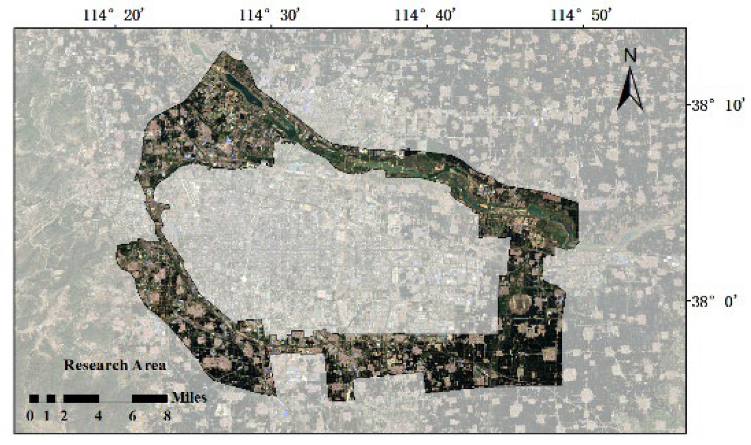
Shijiazhuang, the capital of Hebei Province, is situated in the south-central region of the province and serves as a core city within the world-class Beijing-Tianjin-Hebei urban agglomeration. By the end of 2024, the city’s permanent population reached 11.25 million, including 8.17 million urban residents, resulting in an urbanization rate of 72.66%. Between 2015 and 2024, the central urban area expanded from approximately 278 km² (China City Statistical Yearbook, 2016) to 660 km² (China City Statistical Yearbook, 2021). However, this rapid urban expansion has introduced multiple ecological risks, including encroachment on surrounding green spaces and water systems, occupation of agricultural land, and intensification of the urban heat island effect. To curb this disorderly sprawl, Shijiazhuang designated a 438.0 km² green belt within the urban–rural transition zone between the central urban area and the adjacent counties of Luquan, Luancheng, Gaocheng, and Zhengding. This study focuses on Shijiazhuang’s green belt as the research object. It aims to develop spatial optimization strategies by analyzing the evolution of industrial, ecological, agricultural, service, and residential spaces within the area from 2015 to 2024.
Figure 1.
Scope of the green belt in Shijiazhuang City.
2.2. Research Methods
To address the limitations of single-dimensional quantitative approaches, this study developed a multi-dimensional comprehensive quantitative analysis method. Based on the evolutionary characteristics of different spatial types, five quantitative methods were employed: average nearest neighbor analysis, landscape pattern indices, land-use transfer matrix, kernel density estimation, and spatial autocorrelation. These methods were inte-grated through cross-validation and complementary enhancement to comprehensively reveal the internal mechanisms driving the spatial evolution of green belts and to inform spatial optimization strategies.
2.2.1. Average Nearest Neighbor Analysis(ANN)
Average nearest neighbor analysis determines the amount of spatial clustering or dispersion of point features by comparing the observed mean distance to the expected mean distance if the points were randomly distributed. The formula is expressed as follows:
where: is the average observed distance, ; is the expected average distance,
Most of the previous studies used density based methods to analyze the spatial distribution of industrial spatial distribution, which could not quantitatively interpret the industrial agglomeration or dispersion and the amount of industrial agglomeration or dispersion extent. Therefore, this study used ANN tool in ArcGIS. The significance tests based on the nearest neighbor ratio (R value) and Z score were used to determine whether the spatial distribution of industrial land was clustered, random or dispersed.
2.2.2. Landscape Ecological Index Analysis
- Mean Patch Area (AREA_MN)
The mean patch area represents the average size of all patches of a specific type within the study region (hm²), reflecting the typical scale of patches. A smaller value indicates smaller average patch sizes, suggesting a more fragmented landscape dominated by small patches. The calculation formula is:
where: is the area of the -th patch, and is the total number of patches in this type of landscape.
- 2.
- Standard Deviation of Patch Area (AREA_SD)
This metric measures the standard deviation (hm² or km²) of the patch areas of a particular type within the region, indicating the variability in patch size distribution. Larger values reflect higher variability in patch size, whereas smaller values indicate sizes closer to the mean. The calculation formula is:
where: is the area of the -th patch, and AREA_MN is the average patch area.
- 3.
- Patch Density Index (PD)
The patch density index refers to the number of patches per unit area. It is calculated in two forms: the ratio of ecological patches to the total regional area (PD₁, patches/km²) and the ratio of ecological patches to the ecological land area (PD₂, patches/km²). Higher values suggest greater fragmentation. The calculation formula is:
where: is the total number of patches; is the total area of the landscape.
- 4.
- Largest Patch Index (LPI)
The largest patch index measures the proportion (%) of the largest patch relative to the total landscape area, reflecting the dominance of core patches in the overall landscape pattern. Larger values indicate the presence of dominant, continuous patches, while smaller values suggest fragmentation of core patches. The calculation formula is:
where: is the maximum patch area, and is the total landscape area.
Previous studies on ecological spaces have concentrated on area changes, which hinders an understanding of the internal spatial patterns and structural characteristics. This study uses a correlated set of landscape metrics—mean patch size, standard deviation of patch size, patch density and largest patch index—to characterize the fragmentation of ecological space in green belts of Shijiazhuang from the perspective of scale, variation, degree of fragmentation and dominance of core patches.
2.2.3. Land Use Transfer Matrix Model
The land-use transfer matrix model quantitatively describes the magnitude, direction, and structural characteristics of the mutual transformations among different land-use types within the study area over a specific time interval. The model constructs a two-dimensional matrix that records the area transferred from the -th land-use type to the -th land-use type during different time periods. The dimension of the matrix is determined by the total number of land-use categories n and is expressed as follows:
where: represents the area converted from the -th land use type at the beginning of the period to the -th land use type at the end of the period, and represents the total number of land use types divided in the study area.
Existing studies have primarily focused on net changes in land-use categories, which makes it difficult to reveal the dynamics of conversion between land-use types. By contrast, a land-use transfer matrix captures the direction, pathway, and magnitude of these conversions. In this study, a transfer matrix was constructed for three time periods—2015, 2020, and 2024—to quantify not only the extent of agricultural land encroached upon by built-up land but also the intensity of such conversions at different stages.
2.2.4. Kernel Density Estimation
Kernel density estimation (KDE) treats each observed point as the center of a localized probability mass or influence range. It then calculates the sum of the kernel function values of all point features at any given spatial location x and normalizes this sum to obtain the estimated density at that position.
where: is the kernel density estimate at point ; is the total number of points; is the distance decay threshold; is the kernel function; is the position of the -th observation point.
Previous studies investigating the spatial differentiation of the service industry often used point-of-interest (POI) distribution maps, which are unable to reflect gradual changes in spatial density. This study applies KDE using the raster calculator in ArcGIS to calculate the difference in kernel density between two categories of service industry. By doing so, we are able to illustrate the differentiation process and gain further insights into the spatial evolution of the service industry.
2.2.5. Spatial Autocorrelation Model
- Global Spatial Autocorrelation
This study employs the global Moran’s I index as a core indicator to quantify the degree of spatial clustering or dispersion of POI points within village and town residential spaces. The formula for calculating Moran’s I is as follows:
where: is the total number of spatial cells. and are the attribute values of spatial cell and its neighboring cell , respectively. represents the average of all attribute values of spatial cells. represents the element of the spatial weight matrix, which defines the spatial adjacency relationship between cells and . If cells and are adjacent, = 1; otherwise,= 0.
The value of Moran’s I typically ranges from −1 to 1, and its magnitude reflects both the nature and strength of spatial autocorrelation. Specifically, Moran’s I > 0 indicates positive spatial autocorrelation, meaning that spatial units with similar attribute values tend to cluster together. Moran’s I < 0 suggests negative spatial autocorrelation, indicating that dissimilar units are more likely to be adjacent. Moran’s I ≈ 0 implies no spatial autocorrelation, suggesting that the spatial pattern is nearly random. A larger absolute value corresponds to stronger spatial dependence, reflecting more pronounced clustering or dispersion.
- 2.
- Local Spatial Autocorrelation
Local spatial autocorrelation analysis captures the relationships between the attribute values of spatial units and those of their neighboring units at a localized scale, enabling the identification of specific areas of clustering or spatial anomalies. Local Moran’s I significance maps are generally classified into four spatial association types: High–High and Low–Low, which indicate local spatial clustering, i.e., high-value or low-value areas are concentrated in space. High–Low and Low–High, which indicate local spatial dispersion, i.e., high-value and low-value areas are interspersed in space. The formula for calculating the local Moran’s I index is as follows:
where: represent the index or coupling coordination degree of region and region , which is mainly analyzed through the Local Indicators of Spatial Association cluster diagram.
Related work on the expansion of residential space has mainly focused on statistical analysis of expansion areas or overlay analysis of spatial extent. In contrast, this article proposes using global Moran’s I and local spatial autocorrelation analysis to quantitatively analyze not only the degree of clustering of residential space sprawl but also its temporal characteristics. Based on the LISA cluster maps, we can accurately locate hotspots, lagging areas, and spatial abnormalities in the sprawl process and provide a scientific basis for constructing differential residential space management policies.
2.3. Data Sources
2.3.1. Remote Sensing Image Data and Preprocessing
This study focuses on three key timeframes in Shijiazhuang’s green belts: 2015, 2020, and 2024. Landsat 8–9 OLI/TIRS Collection 2 Level-2 remote sensing imagery, provided by the National Aeronautics and Space Administration (NASA) and the United States Geological Survey (USGS), was acquired from the Geospatial Data Cloud Platform of the Chinese Academy of Sciences (http://www.gscloud.cn/), with a spatial resolution of 30 m × 30 m. Preprocessing was conducted primarily using ArcGIS 10.2 and ENVI 5.3, including image fusion, mosaicking, cropping, and supervised classification.
2.3.2. POI Data and Preprocessing
Point-of-interest (POI) data for Shijiazhuang’s green belts was obtained from the AutoNavi Open Platform (https://lbs.amap.com/). Following the POI data classification standards, five categories were selected for analysis: (1) companies and enterprises, (2) science, education, and cultural services, (3) leisure and entertainment services, (4) lifestyle services, and (5) commercial and residential properties. During preprocessing, the raw POI dataset was cleaned and projected into the WGS84 coordinate system. Duplicate entries and erroneous coordinates were removed, while spatial matching and registration were applied to ensure temporal and spatial consistency across different years. The processed dataset was subsequently reclassified using ArcGIS (Table 1).
3. Results
3.1. Industrial Land: Small and Scattered
Quantitative analysis using landscape ecological indices shows that the mean patch area of industrial land was 11.9646 hm² in 2015, declining to 11.6481 hm² in 2020 and further to 10.2953 hm² in 2024. This indicates a continuous reduction in the size of individual industrial land patches, reflecting the absence of large, contiguous industrial clusters and the predominance of small-scale development. Moreover, the standard deviation of patch area dropped sharply from 248.1834 hm² in 2015 to 121.7657 hm² in 2024, suggesting a substantial decrease in size variation among patches and a more uniform overall distribution. Collectively, these findings demonstrate that industrial land during 2015–2024 was characterized by fragmentation and small-scale dispersion.
Results of the ANN analysis were also supportive of these trends. The calculated mean distance between industrial sites was 598.75 m in 2015 and dropped dramatically to 90.60 m in 2024, which suggested that patches were becoming closer to each other. In addition, the nearest neighbor ratio decreased from 0.413 to 0.080 and the z-score decreased from -11.335 to -33.569 during the same period. Because the ratios were below 1 and the absolute values of the z-scores were larger than 2.58, the two ratios were significantly lower than the corresponding random values, meaning that the patch clustering was not formed by random distribution. In combination with the land-use map (Figure 5), the results revealed that although industrial land presented localized clusters, its overall distribution was dispersed, and therefore presented a fragmented pattern.
In total, industrial land in Shijiazhuang’s green belts expanded steadily from 2015 to 2024, and its spatial configuration was characterized by small and scattered patches. This may be due to two reasons. First, although large industrial parks were forbidden in green belts, as local villages and towns attempted to increase fiscal revenue, they had tacitly tolerated the development of small and micro-scale industries. Second, this scattered distribution enabled industries to obtain land at relatively low cost in ecologically marginal areas and to avoid paying the full cost of infrastructure development. However, the uncontrolled expansion of industrial land also brought about great ecological risks, such as breaking ecological corridors, increasing land surface temperature, enhancing urban heat islands, and causing bare land.

Table 2.
Calculation of Mean Patch Area and Patch Area Standard Deviation of Industrial Land in the Green Belts of Shijiazhuang, 2015–2024.
Table 2.
Calculation of Mean Patch Area and Patch Area Standard Deviation of Industrial Land in the Green Belts of Shijiazhuang, 2015–2024.
| Index | 2015 | 2020 | 2024 |
|---|---|---|---|
| Mean patch area (AREA_MN, hm²) | 11.965 | 11.648 | 10.295 |
| Patch area standard deviation (AREA_SD, hm²) | 248.183 | 158.402 | 121.766 |
Table 3.
Results of Nearest Neighbor Analysis of Industrial Land in the Green Belts of Shijiazhuang, 2015–2024.
Table 3.
Results of Nearest Neighbor Analysis of Industrial Land in the Green Belts of Shijiazhuang, 2015–2024.
| Index | 2015 | 2020 | 2024 |
|---|---|---|---|
| Mean observed distance (m) | 598.751 | 374.671 | 90. 596 |
| Expected random distance (m) | 1448.645 | 1066.842 | 1128.391 |
| Nearest neighbor ratio | 0.413 | 0.351 | 0.080 |
| z-score | -11.335 | -19.309 | -33.569 |
| p-value | 0.000 | 0.000 | 0.000 |
3.2. Fragmentation of Ecological Space
Changes in the Maximum Patch Index (LPI) reflect a marked decline in the size of core ecological patches. The LPI of cultivated land decreased sharply from 19.52% in 2015 to 7.23% in 2020, and further to 6.82% in 2024, indicating a substantial weakening of its role as a continuous, large-scale ecological patch. Grassland showed a fluctuating pattern, with its LPI briefly increasing to 3.03% in 2020 before declining to 1.42% in 2024, suggesting that its capacity to maintain large, stable core patches has also diminished. These results demonstrate that formerly continuous ecological patches have been progressively fragmented and reduced, seriously undermining the connectivity of the ecological space.
As shown in Table 4 and Figure 10, when it comes to the process of leapfrog urbanization, the change trend of patch density (PD) shows the tendency of ecological fragmentation in whole. The PD of cultivated land decreased from 2.069 patches/km² in 2015 to 1.573 patches/km² in 2024. It is not only the fragmentation of large patch but also the breaking away of small patch or merging of small patch into big patch leading to the great decrease of total area. As for forestland, its PD increased greatly from 0.087 patches/km² in 2015 to 1.957 patches/km² in 2020, and the PD decreased slightly in 2024 although, which also reflected the great fragmentation degree. More smaller patches and more fragmented patches were appeared. The PD of grassland decreased firstly and then increased. Combined with the decrease of LPI, it also reflected the fragmentation of remaining or newly added patches, which were small patches and scattered patches.
In summary, the core ecological patches of green belts in Shijiazhuang experienced the process of constant fragmentation in the period from 2015 to 2024. That is, the patches became more and more scattered, more and more small and highly fragmented ecological environment. It was caused by the process of leapfrog urbanization. The built-up land occupied more and more ecological areas around ecological zone. To seek for less cost and better location, the enterprise tended to set the scattered sites around ecological area, which would lead to the phenomenon of ecological fragmentation and degradation.
Table 5.
Statistics of the Ecological Space PD Index in Shijiazhuang’s Green Belts (2015–2024).
| Land Use Type | 2015 | 2020 | 2024 |
|---|---|---|---|
| Cropland | 2.069 | 1.799 | 1.573 |
| Woodland | 0.087 | 1.957 | 1.598 |
| Grassland | 5.010 | 4.921 | 5.311 |
| Water | 0.250 | 0.576 | 0.875 |
3.3. Encroachment on Agricultural Space
Quantitative results from the land-use transition matrix (Table 6) indicate a net decrease of 55.95 ha of cultivated land between 2015 and 2024, with the largest conversion being 24.97 ha transferred to built-up land. The second major transition involved 18.12 ha converted from grassland to built-up land. This process is also evident in the land-use maps: the 2015 map (Figure 2a) shows that cultivated land patches were still large and contiguous, forming the regional agricultural base. Over time, however, built-up land gradually infiltrated and spread across this base (Figure 2b,c). These transformations reveal increasing fragmentation of farmland patches, which—when combined with the scattered distribution of rural settlements—further reduces land-use efficiency.
Stage-specific analysis (Table 7 and Table 8) shows that 2015–2020 period was the year range during which most cultivated land was converted for other uses (net decrease of 73.29 ha). During this stage, 17.51 ha of land were converted to built-up land, which accounted for 23.9% of the decrease in cultivated land. The 2015-2020 land-use map reveals that there were large clusters of built-up land encroaching on the edges of cultivated land. This phenomenon clearly demonstrates the pressure on cultivated land caused by the rapid development of industry.
In contrast, the rate of decrease in cultivated land during 2020–2024 slowed slightly, with a net decrease of 17.34 ha (5.18 ha of land converted to construction, accounting for 29.9%). However, the 2020–2024 land-use map still displays scattered expansion of patches of built-up land, and there are even isolated new developments in the hinterlands of cultivated land that are far away from the built-up area. Therefore, we found that agricultural space was still being eroded.
The continuous erosion of agricultural space within the green belts of Shijiazhuang from 2015 to 2024 indicates a structural problem in the returns from land use. The significantly higher returns per unit of land from industrial land compared with that from agriculture have eroded the internal incentives for local stakeholders to protect farmland. This vicious circle of the fragmentation of farmland and decreasing returns has weakened the agricultural production capacity of the green belts and has become a bottleneck to regional sustainable development.
3.4. Spatial Differentiation of Service Industry Growth
Quantitative analysis based on kernel density estimation reveals pronounced spatial differentiation in the development of cultural–tourism–leisure services versus lifestyle-related services within Shijiazhuang’s green belts between 2015 and 2024. In 2015, high-density clusters of lifestyle-related services were primarily concentrated in the western region, whereas cultural–tourism–leisure services were more dispersed in the northeast. The spatial distribution and intensity of these two sectors differed significantly, suggesting that lifestyle-related services, initially dependent on existing settlements, had a clear first-mover advantage in service coverage. By contrast, cultural–tourism–leisure services, constrained by longer development cycles and limited resource utilization, had not yet established widespread dominance.
Between 2015 and 2020, the spatial pattern of kernel density values underwent notable changes (Figure 3-b). The value range expanded markedly to –318,272.438 to 62,637.084. High-density zones of lifestyle-related services extended southward along major transportation corridors, reflecting their continuous penetration into diversified peri-urban residential spaces. Meanwhile, cultural–tourism–leisure services began to cluster in the northwest, though their expansion remained restricted by uneven resource distribution and slow development progress. The overlap of these clusters with the dispersed expansion of lifestyle-related services further intensified the functional differentiation of regional service industries.
From 2020 to 2024, the spatial differentiation of kernel density values became more pronounced (Figure 3-c), with increasingly complex boundaries between negative-value and positive-value dominated areas. The peak kernel density of cultural–tourism–leisure services rose sharply to 93,955.628–104,395.141, consolidating into a contiguous cluster in the northwest. Driven by rising high-end consumer demand and sustained policy investment in cultural tourism, these services emerged as the core of regional industrial upgrading. In parallel, lifestyle-related services reached very high kernel density values (124,248.489–310,621.219) in newly developed eastern communities, while also maintaining a decentralized distribution across new rural settlements formed under urban expansion to meet livelihood needs.
In summary, the service industry within Shijiazhuang’s green belts evolved from differentiation to interaction between 2015 and 2024. This transformation was shaped by resource endowment, policy orientation, and profit-seeking logic, reflecting the adaptive adjustment of service industries to diversified demand amid rapid urban expansion.
3.5. Spread and Expansion of Residential Space in Villages and Towns
Results of the spatial autocorrelation model revealed that the results of the model indicated the trend of disorderly sprawl and expansion of rural and urban residential space in green belts of Shijiazhuang during 2015–2024. From the macro-agglomeration level, the Global Moran’s I index indicated the overall sprawl of residential space. As shown in Table 3, the Global Moran’s I index was 0.953 in 2015, 0.958 in 2020 and 0.961 in 2024. It indicated that the degree of spatial agglomeration in high-value areas gradually increased. Therefore, the residential distribution pattern changed from “point-like” to “belt-like” and even “surface-like” pattern gradually. Combined with the time-series characteristics of the Moran’s I scatter plots (Figure 4), it can be observed that: in 2015, scatter points were primarily concentrated in the high–high quadrant, reflecting a strong basis of positive spatial correlation; in 2020, scatter points tended to cluster in high-value neighborhoods, indicating that residential space had begun to penetrate surrounding low-value areas; in 2024, scatter points shifted further into the high-value quadrant, highlighting the trend of disorderly spillover and erosion of residential space.
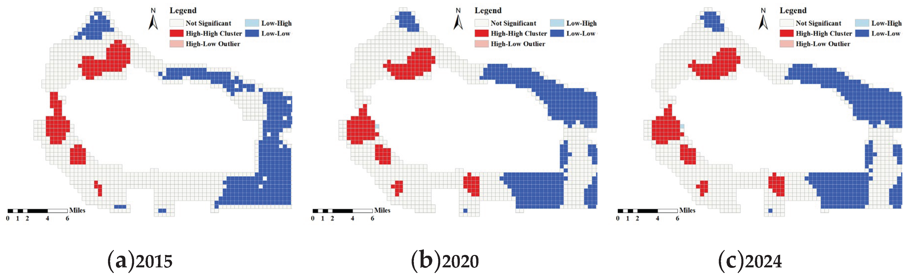
From the micro-level perspective, the 2015 cluster analysis (Figure 5-a) reveals a multi-core, discrete distribution of high–high clusters concentrated in the west and north, forming independent residential patches that began to expand into adjacent low-value areas and laying the foundation for subsequent disorderly growth. Low–low clusters were widely distributed in the east and south, corresponding to areas of non-built-up land. The 2020 cluster analysis (Figure 5-b) shows significant expansion of high–high clusters, which continuously merged with and encroached upon low–low clusters. These clusters extended along transportation corridors and development axes, shifting from a “point-like” to a “belt-like” expansion, gradually encroaching on agricultural and ecological space. This shift was largely driven by employment concentration and the growing residential demand associated with industrial expansion. The 2024 cluster analysis (Figure 5-c) indicates that the high–high clusters in the west and north further merged on a large scale, forming broader and more continuous agglomerations. This process continued to erode low–low clusters, which retreated southeastward and became increasingly fragmented. In addition, leapfrog expansion into ecologically sensitive areas was observed, reflecting a spatial imbalance between saturated residential density in core zones and disorderly sprawl in peripheral areas.
In summary, the steady rise in the Global Moran’s I index confirms the trend of residential space expansion and sprawl. Cluster analysis results clearly demonstrate the transformation of residential space from “island-like dispersion” to “ribbon-like extension” and ultimately to “continuous encroachment.”
Figure 5.
Cluster Analysis of Residential Space in Shijiazhuang’s Green Belts.
4. Conclusion and Discussions
4.1. Conclusion
From 2015 to 2024, the spatial evolution of Shijiazhuang’s green belts was characterized by a “small and scattered” leapfrog expansion of industrial land, the fragmentation of ecological space, continuous encroachment on agricultural space, markedly differentiated growth of service industry space, and the sprawling expansion of residential areas in villages and towns. Due to the imbalance between the rigid constraints of ecological protection and the economic logic of land returns, the benefits of secondary industry far exceeded those of ecology and agriculture, resulting in a “pancake-like” pattern of spatial expansion.
4.1.1. Challenges of “Small and Scattered” Industrial Land Expansion
Between 2015 and 2024, industrial land within Shijiazhuang’s green belts exhibited a “small and scattered” spatial expansion pattern, creating major challenges for infrastructure efficiency, economies of scale, and ecological protection. Smith et al. [3] found that because green belt policies strictly restrict the expansion of contiguous built-up areas, industrial development was forced to adopt a leapfrog expansion model, bypassing the belts for decentralized, low-density development in peripheral zones. This led to negative outcomes such as longer commuting distances, increased automobile dependence, and higher carbon emissions. Hu and Wang [11] used the PLUS model to simulate the impacts of green belt scenarios on ecosystem service values, showing that irrational land-use changes can significantly diminish ecosystem functions. In contrast, Jun [8] employed machine learning simulations and suggested that abolishing the green belt policy could result in more concentrated industrial land within urban cores. Such concentration would not only accommodate larger populations and employment but also reduce the loss of ecological corridor connectivity by up to 20%.
Overall, excessive dispersion of industrial land results in duplicate infrastructure construction, rising commuting costs, and ecological fragmentation. Therefore, while maintaining ecological protection as the foundation, policies should consider local development stages and resource endowments to guide moderate concentration and cluster-based development of industrial land. This would help achieve a dynamic balance between ecological security and industrial growth.
4.1.2. Threats of Ecological Space Fragmentation
From 2015 to 2024, the ecological space in green belts of Shijiazhuang became progressively fragmented. The changes in maximum patch index and patch density represent the connectivity and fragmentation decreasing, and further induce ecological risks including temperature increasing, urban heat island enhancing, vegetation cover decreasing, and high ecological value area diminishing. Do et al. [12] believed that in addition to the direct occupation of a large amount of green space, the rapid urbanization also leads to the degradation of the ecosystem, which seriously affects the sustainable development of the city. Kardani-Yazd et al. [13] believed that the direct fragmentation reduces biodiversity and ecological services. Li et al. [14] believed that the spatial pattern of urban green space has a significant impact on the cooling efficiency, and the layout of fragmentation will greatly weaken the ecological regulation function and aggravate the urban heat island. While Zhou et al. [15] believed that the purpose of the green belt policy in Beijing is to stop the expansion of the city, but due to the poor management and design defects, it has instead caused the internal fragmentation. Different with the fragmentation induced by the process of urbanization in this study.
This fragmentation poses a severe threat to regional ecological security and sustainable development, manifesting in reduced biodiversity, worsened heat island effects, and weakened ecological barriers. Therefore, strengthening ecological connectivity should be prioritized. Constructing wedge-shaped green corridors and integrated blue–green networks would repair fragmented patches, enhance ecological integration, and restore key ecosystem functions.
4.1.3. Threats of Agricultural Space Encroachment
Between 2015 and 2024, eroded agricultural space located in Shijiazhuang’s green belts was continuously decreased. Land-use transfer matrices revealed that the reduction of cultivated land and increasing patch splitting are mainly induced by land return imbalance caused by the rapid development of industry. Han et al. [16] found that the liberalization of green belt policies leads to accelerated conversions of green belts into urban land, causing a large decrease in cultivated land, a serious threat to farmers’ lives and incomes, a challenge to regional food security, and a decrease in the sustainable supply of ecosystem services. Mao et al. [17] studied the farmland loss under various urban expansion patterns in China. They found that the urban sprawl is the main cause of the occupation of agricultural space, and called for relevant policy interventions. However, it is not easy to implement protective policies. Akimowicz et al. [18] believed that governments need to create multifunctional agricultural models under strict land conditions and seek efficient ways to balance ecological conservation and agricultural development. In addition, Porter et al. [19] warned that farmland protection policies that offer economic incentives may lead to “fake protection” of farmland. That is, the land on the books is protected but poorly managed, offering little ecological or productive service.
These findings suggest that agricultural protection policies must fully account for the imbalance in land-use benefits. Promoting multifunctional agricultural models is essential to achieving coordinated ecological conservation and agricultural productivity. At the same time, safeguards must be established against “false protection,” ensuring that preserved farmland retains both ecological and production value.
4.1.4. Challenges of Spatially Differentiated Service Industry Growth
From 2015 to 2024, the service industry within Shijiazhuang’s green belts displayed pronounced spatial differentiation, with both cultural–tourism–leisure services and livelihood-supporting services following dispersed evolutionary trajectories. Zhao et al. [20] noted that external service facilities, such as cultural amenities, significantly enhance leisure utilization intensity in green belts, indicating that the spatial distribution of cultural and tourism services strongly shapes the functional performance of surrounding green space. Liu et al. [21] highlighted the ecological services of green belts, particularly their irreplaceable role in mitigating urban noise and improving quality of life. Conversely, Smith [3], based on the London case, argued that concentrated service industry layouts, though market-driven and economically efficient, often occur at the expense of ecological land.
This evidence underscores that spatially differentiated growth of the service industry has profound implications for balancing functional coordination and ecological protection. Policy frameworks must therefore reconcile ecological protection with dynamic livelihood needs, and market efficiency with regulatory guidance, to achieve multi-objective coordination among ecological conservation, livelihood security, and economic benefits.
4.1.5. Challenges of Residential Space Sprawl and Expansion
Between 2015 and 2024, residential space in Shijiazhuang’s villages and towns within the green belts exhibited continuous sprawl, as reflected in the steadily rising global Moran’s I. Cluster analysis revealed that “high–high” clusters evolved from multi-core discreteness to large-scale contiguous agglomerations, intensifying challenges to ecological connectivity, infrastructure capacity, and social equity. Wei et al. [22], in a study of suburban Wuhan, proposed a comprehensive evaluation framework showing that low-density, sprawling residential expansion leads to socioeconomic inefficiency and ecological service loss, a finding consistent with this study. However, Ma and Jin [10] emphasized that while strict green belt policies may restrain sprawl, they can also excessively compress residential development into limited corridors, producing uncontrolled density and infrastructure overload in transport, water, and energy systems.
Thus, although sprawling residential expansion may temporarily satisfy housing demand, it undermines ecological connectivity, encroaches on farmland, and aggravates infrastructure deficiencies. To address these issues, residential development should be guided toward moderate intensification, avoiding disorderly sprawl in villages and towns. Comprehensive spatial strategies must balance ecological constraints, infrastructure capacity, and residents’ livelihood needs to achieve sustainable residential land use.
4.2. Policy Recommendations
To address the contradictions between ecological protection and urban expansion within Shijiazhuang’s green belts, a spatial governance strategy of “adjust one, limit two, and develop three” is proposed. This approach emphasizes the integration of ecological space, the intensive utilization of residential space, and the optimization of land-use functions, aiming to ensure the long-term, orderly, and sustainable development of Metropolis green belts.
4.2.1. Enhancing the Value of Agricultural Space
Guided by the “one adjustment” principle, agricultural spatial layout should be optimized to transform agriculture from a single-function system into a multifunctional model, shifting farmland from passive erosion to proactive value creation. Promoting high-value-added, green, and sustainable agricultural practices can increase farmers’ incomes, thereby reducing economic pressures that drive the conversion of farmland to non-agricultural uses. Improving the allocation and efficiency of agricultural resources is essential, particularly through the development of modern agricultural industrial parks. By consolidating fragmented farmland into contiguous cultivation zones and integrating production, processing, and leisure services, agricultural space can achieve higher land-use efficiency and greater ecological and economic benefits.
4.2.2. Aggregating Industrial Space
Following the “two limitations” strategy, the disorderly proliferation of dispersed industries must be curbed by redirecting industrial development toward spatial concentration. Establishing clear boundaries for industrial agglomeration and enforcing a “negative list” for industrial land within green belts are crucial steps to gradually phase out highly polluting, low-efficiency small-scale industries. Such measures address the root causes of leapfrog industrial expansion that threatens ecological land. At the same time, promoting the clustering of high-value-added and R&D-intensive industries within designated industrial parks can strengthen economies of scale, improve land-use efficiency, and enhance the ecological compatibility of industrial activities.
4.2.3. Coordinating Service Industry Development
In line with the “three developments” approach, service industry space should be diversified and spatially balanced to reconcile livelihood needs with ecological protection. Ensuring equitable distribution of livelihood-supporting services can prevent overconcentration in core areas while extending services to underserved regions. Leveraging the ecological assets of green belts, low-intrusion and ecologically adaptive cultural tourism and leisure industries should be promoted. By adopting “park-like” renewal concepts, cultural and tourism facilities can be embedded within ecological networks, fostering the organic integration of cultural, ecological, and agricultural spaces. This strategy not only enhances the service functions of green belts but also supports their ecological and social sustainability.
4.2.4. Integrating Ecological Space
A systematic approach to ecological space integration is essential for strengthening the structural and functional stability of ecosystems. Connectivity among ecological corridors should be enhanced to establish resilient and adaptive ecological networks. Rivers and woodlands can serve as the backbone of such networks, forming ecological corridors and connectivity systems that safeguard biodiversity and landscape resilience. By applying “wedge-shaped green corridors” and “blue–green networks,” fragmented ecological patches can be reconnected, scattered ecological lands integrated, and the integrity and continuity of the regional ecological landscape significantly improved.
4.2.5. Intensifying Residential Space
Residential development should follow a model of concentrated distribution to reduce inefficient land consumption and align housing expansion with industrial layout and ecological carrying capacity. Efforts should focus on concentrating rural and town residential areas within core township centers or along transportation corridors, where public service infrastructure can be efficiently provided. Expansion into ecologically sensitive zones and contiguous farmland must be strictly prohibited to prevent the degradation of ecological and agricultural functions. At the same time, leapfrog residential development in marginal areas should be curbed to enhance land-use efficiency and ensure that residential growth is both spatially rational and environmentally sustainable.
4.3. Research Prospects
At the data level, this study employed remote sensing images and POI data from three time periods (2015, 2020 and 2024) to obtain overall trends and staged characteristics of spatial evolution of green belts in Shijiazhuang. However, due to the absence of continuous annual data, it was difficult to detect the process of change and transitional details. Therefore, future studies should develop continuous time-series datasets to detect critical transition points more accurately and assess the timeliness and effectiveness of policies in the long term.
At the analytical level, due to limitations in interdisciplinary expertise and data availability, a supporting economic analysis framework could not be established, which limited our ability to assess fiscal costs and benefits, market responses and social welfare effects of spatial policy implementation. Therefore, future studies should adopt an interdisciplinary approach involving land economics, urban planning and public policy evaluation to establish a coupled “policy–space–economy” analytical model to simulate different policy scenarios, which would improve the robustness of policy design and provide better economic justification for spatial governance policies.
Author Contributions
Conceptualization, Xiong Guoping; Methodology, Xiong Guoping; Software, Yao Zhuowei; Validation, Xiong Guoping and Yao Zhuowei; Formal Analysis, Yao Zhuowei; Investigation, Xiong Guoping; Resources, Xiong Guoping; Data Curation, Xiong Guoping; Writing—Original Draft Preparation, Yao Zhuowei; Writing—Review & Editing, Xiong Guoping; Visualization, Xiong Guoping; Supervision, Xiong Guoping; Project Administration, Xiong Guoping; Funding Acquisition, Xiong Guoping. All authors have read and agreed to the published version of the manuscript.
Funding
This research was funded by National Key R&D Program of China, grant number 2023YFC3806000, 2023YFC38060004, and Tibet Cultural Heritage and Development Collaborative Innovation Center, grant number XT-ZB202301.
Data Availability Statement
The data that support the findings of this study are partly publicly available. Remote sensing images were obtained from the Geospatial Data Cloud Platform of the Chinese Academy of Sciences (http://www.gscloud.cn/), with Landsat 8–9 OLI/TIRS Collection 2 Level-2 imagery provided by NASA and the United States Geological Survey (USGS). Point-of-interest (POI) data were obtained from the AutoNavi Open Platform (https://lbs.amap.com/). Statistical data were derived from the China City Statistical Yearbook (2016, 2021 editions). The processed datasets generated and analyzed during the current study are available from the corresponding author upon reasonable request.
Acknowledgments
The authors sincerely acknowledge the provision of remote sensing data from the United States Geological Survey (USGS, Landsat imagery) and the European Space Agency (ESA, Sentinel data), as well as point-of-interest (POI) datasets obtained from the Amap (Gaode Map) platform. We also express our sincere gratitude to the Shijiazhuang Planning Bureau for their valuable support and assistance throughout this study. The constructive comments and suggestions from the anonymous reviewers and editors are highly appreciated.
Conflicts of Interest
The authors declare no conflicts of interest. The funders had no role in the design of the study; in the collection, analyses, or interpretation of data; in the writing of the manuscript; or in the decision to publish the results.
References
- Zhan, F.; Liu, Z.; Wang, B. Study on the Spatiotemporal Evolution of the “Contraction–Expansion” Change of the Boundary Area between Two Green Belts in Beijing Based on a Multi-Index System. Land 2023, 12, 1621. [Google Scholar] [CrossRef]
- Pourtaherian, P.; Jaeger, J.A. How Effective Are Greenbelts at Mitigating Urban Sprawl? A Comparative Study of 60 European Cities. Landscape and Urban Planning 2022, 227, 104532. [Google Scholar] [CrossRef]
- Smith, D.A. Travel Sustainability of New Build Housing in the London Region: Can London’s Green Belt Be Developed Sustainably? Cities 2025, 156, 105574. [Google Scholar] [CrossRef]
- Walton, W. A Comment on Michael Pacione’s ‘The Power of Public Participation in Local Planning in Scotland: The Case of Conflict over Residential Development in the Metropolitan Green Belt’. GeoJournal 2019, 84, 545–553. [Google Scholar] [CrossRef]
- Dockerill, B.; Sturzaker, J. Green Belts and Urban Containment: The Merseyside Experience. Planning Perspectives 2020. [Google Scholar] [CrossRef]
- Eswar, M. The Green Belt Of Bangalore: Planning And The Socio-Economic Context. Theoretical and Empirical Researches in Urban Management 2021, 16, 21–38. [Google Scholar]
- Choi, C.G.; Lee, S.; Kim, H.; Seong, E.Y. Critical Junctures and Path Dependence in Urban Planning and Housing Policy: A Review of Greenbelts and New Towns in Korea’s Seoul Metropolitan Area. Land Use Policy 2019, 80, 195–204. [Google Scholar] [CrossRef]
- Jun, M.-J. Simulating Seoul’s Greenbelt Policy with a Machine Learning-Based Land-Use Change Model. Cities 2023, 143, 104580. [Google Scholar] [CrossRef]
- Lee, S.; Yoon, H. Effects of Greenbelt Cancellation on Land Value: The Case of Wirye New Town, South Korea. Urban Forestry & Urban Greening 2019, 41, 55–66. [Google Scholar] [CrossRef]
- Ma, M.; Jin, Y. Economic Impacts of Alternative Greenspace Configurations in Fast Growing Cities: The Case of Greater Beijing. Urban Studies 2019, 56, 1498–1515. [Google Scholar] [CrossRef]
- Hu, Z.; Wang, S. Multi-Scenario Simulation of Ecosystem Service Value in Beijing’s Green Belts Based on PLUS Model. Land 2025, 14, 408. [Google Scholar] [CrossRef]
- Do, D.T.; Huang, J.; Cheng, Y.; Truong, T.C.T. Da Nang Green Space System Planning: An Ecology Landscape Approach. Sustainability 2018, 10, 3506. [Google Scholar] [CrossRef]
- Kardani-Yazd, N.; Kardani-Yazd, N.; Mansouri Daneshvar, M.R. Strategic Spatial Analysis of Urban Greenbelt Plans in Mashhad City, Iran. Environ Syst Res 2019, 8, 30. [Google Scholar] [CrossRef]
- Li, J.; Wang, H.; Cai, X.; Liu, S.; Lai, W.; Chang, Y.; Qi, J.; Zhu, G.; Zhang, C.; Liu, Y. Quantifying Urban Spatial Morphology Indicators on the Green Areas Cooling Effect: The Case of Changsha, China, a Subtropical City. Land 2024, 13, 757. [Google Scholar] [CrossRef]
- Zhou, L.; Gong, Y.; López-Carr, D.; Huang, C. A Critical Role of the Capital Green Belt in Constraining Urban Sprawl and Its Fragmentation Measurement. Land Use Policy 2024, 141, 107148. [Google Scholar] [CrossRef]
- Han, H.; Huang, C.; Ahn, K.-H.; Shu, X.; Lin, L.; Qiu, D. The Effects of Greenbelt Policies on Land Development: Evidence from the Deregulation of the Greenbelt in the Seoul Metropolitan Area. Sustainability 2017, 9, 1259. [Google Scholar] [CrossRef]
- Mao, C.; Feng, S.; Zhou, C. Cropland Loss Under Different Urban Expansion Patterns in China (1990–2020): Spatiotemporal Characteristics, Driving Factors, and Policy Implications. Land 2025, 14, 343. [Google Scholar] [CrossRef]
- Akimowicz, M.; Képhaliacos, C.; Landman, K.; Cummings, H. Planning for the Future? The Emergence of Shared Visions for Agriculture in the Urban-Influenced Ontario’s Greenbelt, Canada, and Toulouse InterSCoT, France. Reg Environ Change 2020, 20, 57. [Google Scholar] [CrossRef]
- Porter, A.; Berrens, R.P.; Fleck, J. New Mexico’s Greenbelt Law: Disincentivizing Water Conservation Through Agricultural Tax Breaks. Nat. Res. J. 2023, 63, 1. [Google Scholar]
- Zhao, W.; Wang, Y.; Chen, D.; Wang, L.; Tang, X. Exploring the Influencing Factors of the Recreational Utilization and Evaluation of Urban Ecological Protection Green Belts for Urban Renewal: A Case Study in Shanghai. International Journal of Environmental Research and Public Health 2021, 18, 10244. [Google Scholar] [CrossRef]
- Liu, L.; Han, B.; Tan, D.; Wu, D.; Shu, C. The Value of Ecosystem Traffic Noise Reduction Service Provided by Urban Green Belts: A Case Study of Shenzhen. Land 2023, 12, 786. [Google Scholar] [CrossRef]
- Wei, J.; Tian, Y.; Li, C.; Yuan, H.; Liu, Y. The Coordinative Evaluation of Suburban Construction Land from Spatial, Socio-Economic, and Ecological Dimensions: A Case Study of Suburban Wuhan, Central China. Land 2025, 14, 900. [Google Scholar] [CrossRef]
Figure 2.
Land-Use Maps of Green Belts in Shijiazhuang.
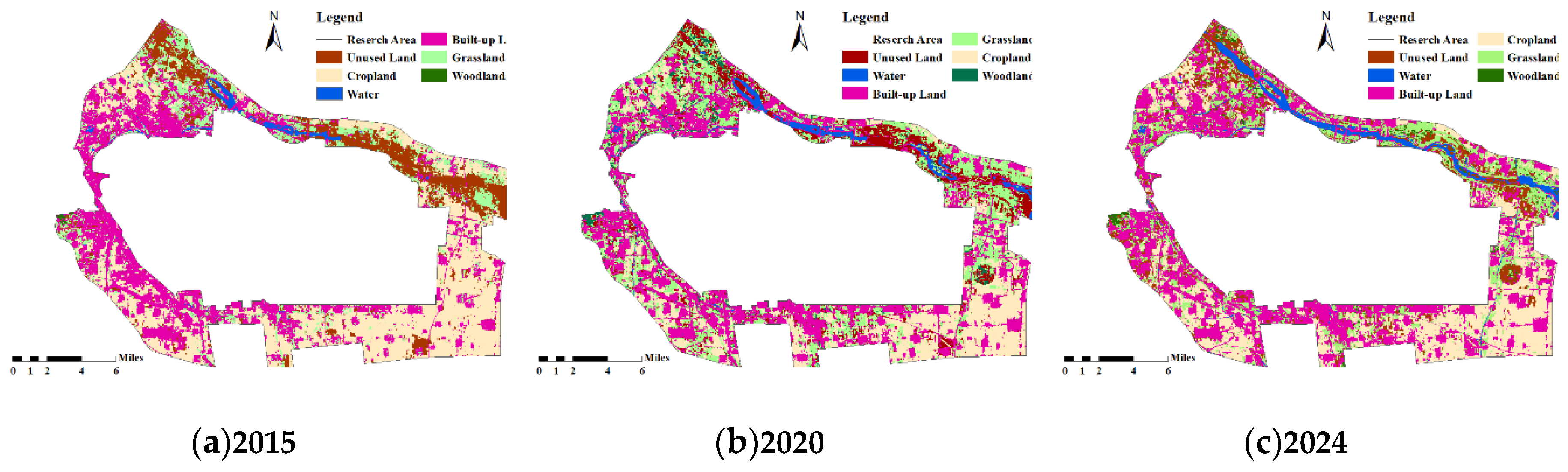
Figure 3.
Spatial Kernel Density Difference Analysis of the Service Industry in Shijiazhuang’s Green Belts.
Figure 3.
Spatial Kernel Density Difference Analysis of the Service Industry in Shijiazhuang’s Green Belts.
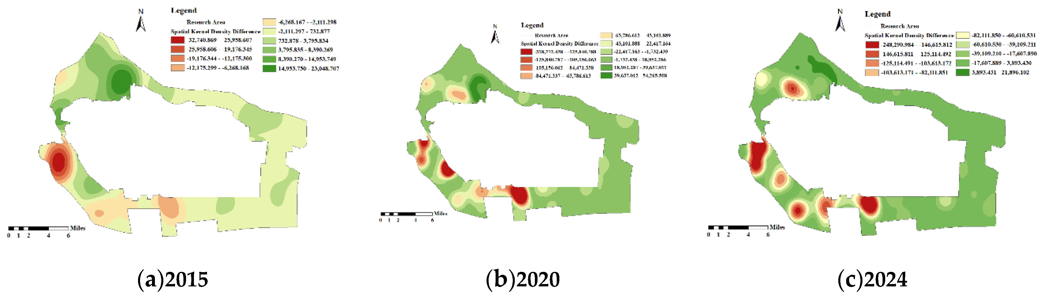
Figure 4.
Scatter Plots of the Global Moran’s I Index of Residential Space in Shijiazhuang’s Green Belts.
Figure 4.
Scatter Plots of the Global Moran’s I Index of Residential Space in Shijiazhuang’s Green Belts.
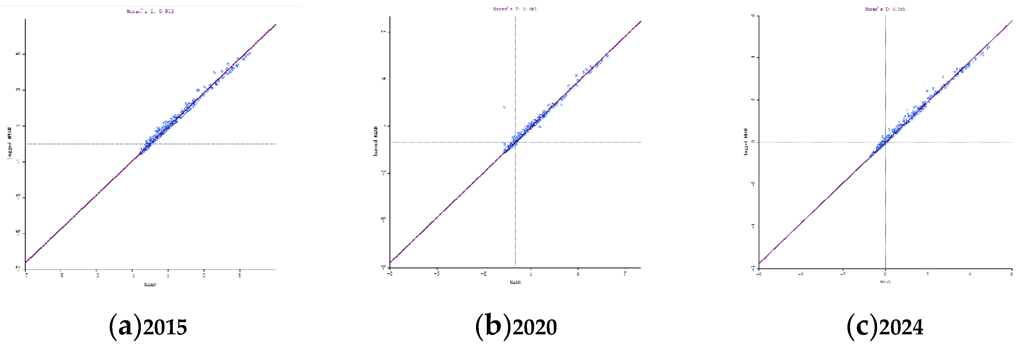
Table 1.
Reclassification of POI Data.
| Spatial Category | Primary POI Classification | Secondary POI Classification |
|---|---|---|
| Industrial Space | Companies and Enterprises | Factories |
| Service Industry Space-Cultural Tourism and Leisure Oriented Services | Science, Education, Culture, Leisure, and Entertainment | Museums, science and technology museums, archives, libraries, cultural centers, radio and television stations, cinemas, karaoke (KTV) venues, retirement and holiday centers, bars, agritourism farmhouses, chess and card rooms, internet cafés, amusement parks, etc. |
| Service Industry Space-Life Supporting Services | Lifestyle Services | Public utilities, post offices, agencies and intermediaries, lottery outlets, logistics, photography and printing services, beauty and hairdressing salons, information and consultation centers, etc. |
| Living Space | Commercial and Residential Properties | Village and town residential areas |
Table 4.
Statistics of the Ecological Space LPI Index in Shijiazhuang’s Green Belts (2015–2024).
| Land Use Type | 2015 | 2020 | 2024 |
|---|---|---|---|
| Cropland | 19.52% | 7.23% | 6.82% |
| Woodland | 0.07% | 0.23% | 0.23% |
| Grassland | 0.92% | 3.03% | 1.42% |
| Water | 0.50% | 0.59% | 1.16% |
Table 6.
Land-Use Transfer Matrix of Green Belts in Shijiazhuang (2015–2024).
| Land Use Type | Cropland | Woodland | Grassland | Water | Built-up Land | Unused Land | Total | Area Change |
|---|---|---|---|---|---|---|---|---|
| Cropland | 103.89 | 0.00 | 4.14 | 0.00 | 6.04 | 3.70 | 117.77 | 55.95 |
| Woodland | 1.31 | 0.66 | 2.69 | 0.05 | 1.25 | 2.07 | 8.04 | -7.16 |
| Grassland | 31.84 | 0.07 | 24.01 | 0.08 | 17.26 | 16.67 | 89.93 | -30.23 |
| Water | 0.24 | 0.01 | 1.30 | 6.15 | 3.82 | 9.93 | 21.45 | -14.49 |
| Built-up Land | 24.97 | 0.08 | 18.12 | 0.65 | 106.01 | 15.93 | 165.75 | -23.97 |
| Unused Land | 11.48 | 0.07 | 9.43 | 0.03 | 7.40 | 16.77 | 45.17 | 19.91 |
| Total | 173.72 | 0.88 | 59.69 | 6.96 | 141.78 | 65.08 | 448.12 | |
| Area Change | -55.95 | 7.16 | 30.23 | 14.49 | 23.97 | -19.91 |
* Note: Vertical data represent land-use types in 2015, and horizontal data represent land-use types in 2024. The area unit is hectares (ha).
Table 7.
Land-Use Transfer Matrix of Green Belts in Shijiazhuang (2015–2020).
| Land Use Type | Cropland | Woodland | Grassland | Water | Built-up Land | Unused Land | Total | Area Change |
|---|---|---|---|---|---|---|---|---|
| Cropland | 93.92 | 0.00 | 1.99 | 0.00 | 2.78 | 1.74 | 100.43 | 73.29 |
| Woodland | 1.78 | 0.70 | 4.40 | 0.13 | 2.69 | 2.37 | 12.06 | -11.18 |
| Grassland | 49.66 | 0.06 | 27.40 | 0.01 | 19.08 | 20.51 | 116.73 | -57.04 |
| Water | 0.19 | 0.01 | 0.58 | 6.33 | 2.70 | 4.28 | 14.09 | -7.12 |
| Built-up Land | 17.51 | 0.05 | 14.20 | 0.44 | 105.71 | 11.43 | 149.33 | -7.55 |
| Unused Land | 10.66 | 0.07 | 11.13 | 0.05 | 8.81 | 24.75 | 55.48 | 9.60 |
| Total | 173.72 | 0.88 | 59.69 | 6.96 | 141.78 | 65.08 | 448.12 | |
| Area Change | -73.29 | 11.18 | 57.04 | 7.12 | 7.55 | -9.60 |
* Note: Vertical data represent land-use types in 2015, and horizontal data represent land-use types in 2020. The area unit is hectares (ha).
Table 8.
Land-Use Transfer Matrix of Green Belts in Shijiazhuang (2020–2024).
| Land Use Type | Cropland | Woodland | Grassland | Water | Built-up Land | Unused Land | Total | Area Change |
|---|---|---|---|---|---|---|---|---|
| Cropland | 85.31 | 0.66 | 24.26 | 0.01 | 4.25 | 3.28 | 117.77 | -17.34 |
| Woodland | 0.08 | 2.25 | 2.96 | 0.10 | 0.57 | 2.07 | 8.04 | 4.02 |
| Grassland | 6.64 | 3.70 | 49.69 | 0.27 | 12.38 | 17.24 | 89.93 | 26.80 |
| Water | 0.01 | 0.56 | 1.32 | 12.13 | 3.20 | 4.23 | 21.45 | -7.37 |
| Built-up Land | 5.18 | 1.81 | 18.47 | 1.53 | 125.15 | 13.63 | 165.75 | -16.43 |
| Unused Land | 3.21 | 3.08 | 20.03 | 0.05 | 3.78 | 15.02 | 45.17 | 10.31 |
| Total | 100.43 | 12.06 | 116.73 | 14.09 | 149.33 | 55.48 | 448.12 | |
| Area Change | 17.34 | -4.02 | -26.80 | 7.37 | 16.43 | -10.31 |
* Note: Vertical data represent land-use types in 2020, and horizontal data represent land-use types in 2024. The area unit is hectares (ha).
Disclaimer/Publisher’s Note: The statements, opinions and data contained in all publications are solely those of the individual author(s) and contributor(s) and not of MDPI and/or the editor(s). MDPI and/or the editor(s) disclaim responsibility for any injury to people or property resulting from any ideas, methods, instructions or products referred to in the content. |
© 2025 by the authors. Licensee MDPI, Basel, Switzerland. This article is an open access article distributed under the terms and conditions of the Creative Commons Attribution (CC BY) license (http://creativecommons.org/licenses/by/4.0/).
Copyright: This open access article is published under a Creative Commons CC BY 4.0 license, which permit the free download, distribution, and reuse, provided that the author and preprint are cited in any reuse.


