

Submitted:
13 September 2025
Posted:
16 September 2025
You are already at the latest version
Abstract
Employee attrition imposes high financial and organizational costs, with preventable departures typically far more expensive than false alarms. This study frames attrition prediction as a decision-support problem and introduces a leakage-aware framework that leverages LLM-based augmentation to generate realistic minority-class samples. Using the IBM HR dataset, we benchmark classical, tree-based, transformer, and AutoML models. Results show that LLM-based augmentation consistently improves recall of potential leavers, even when AUC or Average Precision remain statistically unchanged. From a managerial perspective, higher recall enables organizations to prevent more costly departures at the expense of only modest increases in false positives, producing a favorable cost–benefit balance. SHAP analyses confirm that key drivers such as overtime, mobility, and job satisfaction remain interpretable and actionable, while fairness analysis shows small subgroup disparities, supporting equitable deployment. Overall, the proposed framework demonstrates how leakage-aware, recall-oriented augmentation can translate generative AI advances into transparent, fair, and decision-relevant tools for HR retention, with potential applicability to other rare-event domains such as churn, fraud, and risk prediction.
Keywords:
employee attrition
; decision support
; HR analytics
; cost savings
; interpretability
; fairness
1. Introduction
Employee attrition creates a decision problem with asymmetric costs. HR leaders must allocate limited retention budgets under uncertainty and trade off missed preventable departures against avoidable interventions. Credible industry evidence estimates replacement costs at about – annual salary per role, totaling roughly USD 1 trillion per year in the U.S. [1]. We therefore frame attrition prediction as decision support. A useful model prioritizes the minority class (Attrition=Yes) at tolerable false-alarm rates, produces interpretable outputs that guide action, and supports equitable decisions across subgroups.
A practical barrier is that widely used HR datasets are small and highly imbalanced. A common shortcut—“balance then split” (e.g., oversampling before cross-validation or a hold-out split)—leaks target information across folds and biases estimates, especially for small tabular data [2]. Reproducibility checklists in leading venues also call for explicit disclosure of data handling and leakage controls [3]. These points motivate leakage-aware evaluation for any augmentation that seeks to improve minority recall and the precision–recall trade-off.
Recent progress in LLM-based augmentation offers a principled augmentation route. GReaT encodes rows as text, fine-tunes an autoregressive transformer, and supports arbitrary conditioning to sample realistic rows that capture cross-feature dependencies [4]. We apply conditional sampling strictly within training folds to synthesize minority instances without breaking out-of-fold integrity, aiming to improve decision-relevant metrics.
1.1. Related Work
We review methods for class imbalance, LLM-based augmentation, and standards for interpretability, fairness, and rigorous evaluation. Classical remedies such as SMOTE/ADASYN and tabular GANs appear frequently in HR analytics; however, unless resampling remains strictly in-fold, these methods induce optimistic bias via leakage [2]. In contrast, LLM-based augmentation (e.g., GReaT) model joint dependencies over textual encodings and enable arbitrary conditioning without bespoke retraining, making them suitable for principled augmentation when applied in-fold [4].
For transparency, SHAP is a common choice to attribute predictions to features and to translate them into actionable managerial levers [30]. To assess equity, we follow the equal opportunity criterion and report true positive rate (TPR) gaps across demographic subgroups [29]. For rigorous comparison, we pair ROC-AUC/PR-AUC with statistical tests for AUC differences (e.g., DeLong) when appropriate.
1.2. Research Gap
From a decision perspective, the literature lacks:
- 1.
- Leakage-free, decision-relevant evaluations of LLM-based augmentation on highly imbalanced HR data, with metrics and summaries aligned to asymmetric costs and budget constraints;
- 2.
- Head-to-head evidence on how classical ML versus a compact transformer–MLP exploit synthetic minority samples under identical, leakage-controlled protocols;
- 3.
- Demonstrations that numeric gains translate into interpretable, actionable, and fair decisions (higher minority recall at tolerable false-alarm rates, SHAP levers mapping to HR actions, and bounded subgroup TPR gaps);
- 4.
- Systematic analysis of synthetic scale effects (progressive augmentation) to guide budgeted deployment.
1.3. Our Contributions
- Decision-centric LLM augmentation. We adapt GReaT-style conditional generation [4] to synthesize minority (Attrition=Yes) records strictly within training folds, select models on validation folds, and leave test folds untouched, with the goal of reducing costly false negatives.
- Dual benchmark suite and statistics. We compare logistic and boosted-tree baselines to a compact transformer–MLP; we report ROC-AUC, PR-AUC, balanced accuracy, and decision-facing summaries (alerts per true save), and apply DeLong tests for AUC differences across seeds.
- Progressive augmentation guidance. We trace performance and intervention load across synthetic scales (e.g., to the minority count) and identify robust operating regions for practice.
- Open artifacts. We release code, prompts, and configs to support reproduction consistent with community checklists [3].
1.4. Paper Structure
Section 2 describes datasets and the GReaT-based generation pipeline. Section 3 reports results under leakage control, including progressive augmentation. Section 4 interprets decision impacts, subgroup fairness, and ethics. Section 5 concludes and outlines deployment-oriented next steps aligned with MDPI’s DSAM emphasis on bridging methods and managerial decision-making [28].
2. Materials and Methods
2.1. Dataset and Preprocessing
We use the IBM HR Attrition dataset (about 1.5k employees) with demographic, performance, and workplace factors and a binary attrition label (“Yes”/“No”). The minority (“Yes”) rate is roughly 15–17%, which makes both learning and evaluation non-trivial[31].
As Figure 1 shows, we avoid leakage by fitting all preprocessing on the training split only and then applying it to validation/test. We standardize numerical features and one-hot encode categorical features using a standard transformer stack[5,6]. We adopt a stratified 70/30 train–test split with a fixed random seed to preserve class ratios across runs[7,8].
To illustrate class overlap, we project the training set into two dimensions using PCA and t-SNE. PCA gives a linear projection that retains maximum variance; t-SNE provides a non-linear, neighborhood-preserving view for exploration[10,11,12,13]. As shown in Figure 2, attriting and non-attriting employees intermingle instead of forming a distinct cluster. Single drivers (e.g., OverTime, JobSatisfaction) cannot fully separate the classes, which suggests that higher-capacity models and augmentation may help.
2.2. Synthetic Data Generation
To address class imbalance, we synthesize minority (Attrition=Yes) samples via LLM-based augmentation. We adopt GReaT (Generation of Realistic Tabular data)[4], which fine-tunes an autoregressive LLM on text-encoded rows and supports fully-conditional sampling. All fitting and sampling occur strictly within training folds to keep evaluation leakage-free.
LLM setup.
We fine-tune a distilled transformer (∼1.5B parameters) on the training split’s positive cases using LoRA adapters (low-rank updates with frozen base weights) to cut trainable parameters and memory. After up to 100 epochs, we sample additional “Yes” instances. For diversity and control, we enable guided sampling (feature-by-feature generation) with a random feature order and temperature , which GReaT recommends for wide, mixed-type tables.
Scale of augmentation and validity checks.
We add and synthetic “Yes” records (about and oversampling of the minority class) to the original training data. We apply schema/range checks (e.g., nonnegative age and working years), de-duplicate near-duplicates, and drop any constraint violations before training.
CTGAN baseline.
For comparison, we train a CTGAN baseline on the same in-fold training data using ydata-synthetic[16]. We set epochs, latent/embedding, generator dims, critic dims, PAC, batch, and Adam with learning rate and . CTGAN uses conditional vectors and training-by-sampling for imbalanced discrete columns and mode-specific normalization for non-Gaussian continuous features[25]. We monitor generator/critic losses, checkpoint the best model, and use conservative early stopping. Relative to CTGAN, the GReaT pipeline is operationally simpler (no adversarial dynamics or heavy retuning) while retaining fully-conditional sampling.
2.3. Predictive Models and Training
We evaluate five classifiers:
All models use the same training split. Baselines train on original data; augmentation runs refit on the augmented set (original + synthetic). For LR we set class_weight=’balanced’; for XGBoost we tune scale_pos_weight; for RF we downsample the majority class within each bootstrap draw. We select hyperparameters (e.g., LR regularization, XGBoost depth/learning rate) by grid search with 5-fold stratified cross-validation optimizing ROC-AUC; AutoGluon performs its own internal tuning. No model accesses any information about the “Attrition” label beyond its training data[19,23,24].
2.4. Evaluation Metrics
We evaluate discrimination, fairness, calibration, interpretability, and augmentation scalability.
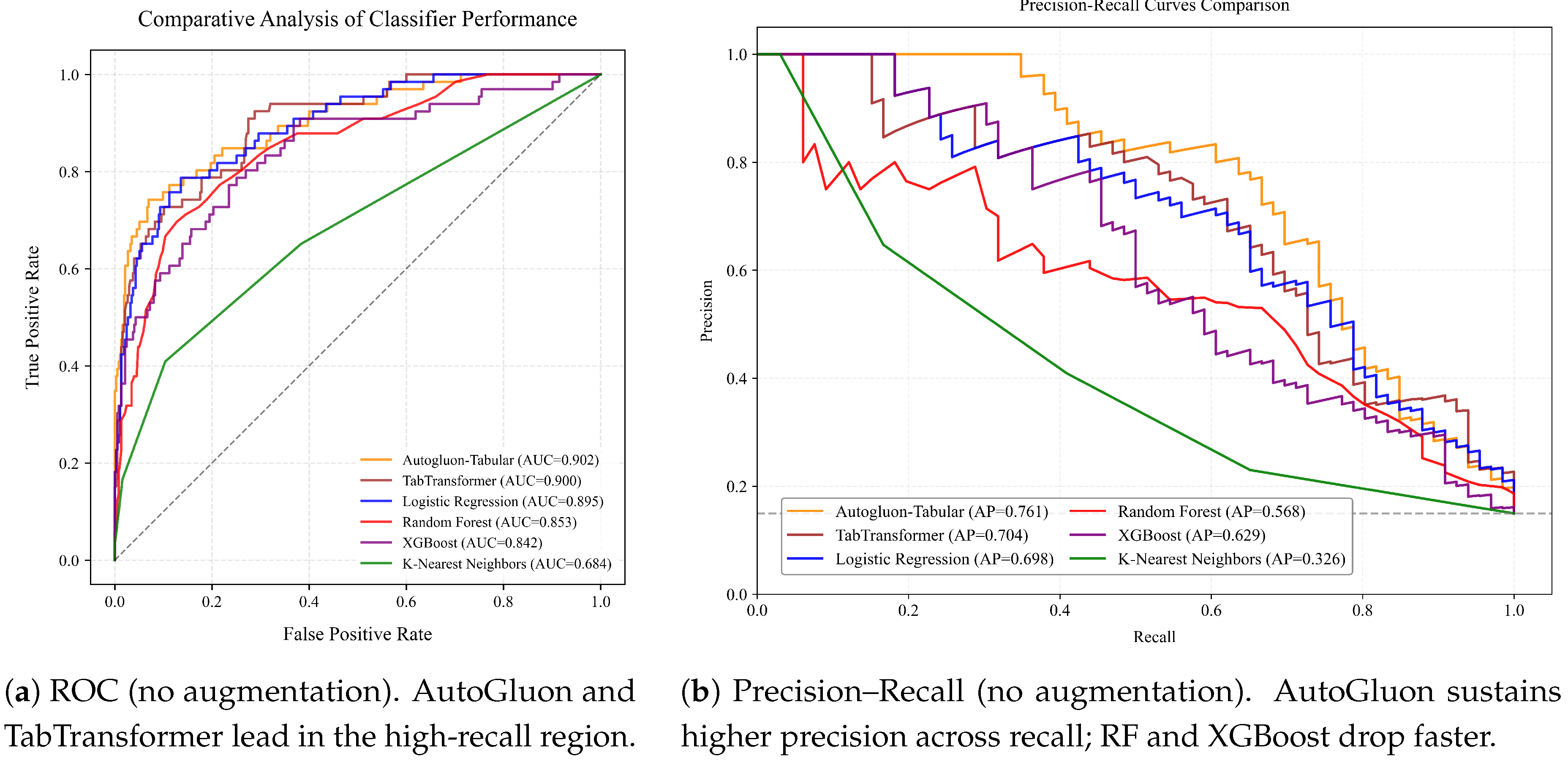
- Discrimination. We report ROC-AUC and Average Precision (AP; area under the Precision–Recall curve[39]) on the test set and plot ROC and PR curves (Figure 3(b)). PR curves emphasize minority-class performance when positives are rare[38,42]. We also show a confusion matrix for the best model (Figure 4(a)) and derive precision and recall for the attrition class. In PR space, the no-skill baseline is a horizontal line at the positive prevalence (here ), and AP measures improvement over this baseline.
- Fairness. Following equal opportunity, we compute the true positive rate (TPR) for females and males and report the TPR gap on the test set[29]. We do not impose fairness constraints; this diagnostic surfaces potential bias. Because base attrition rates differ slightly by gender, we report groupwise TPRs alongside the gap.
- Interpretability. We use SHAP to attribute predictions and summarize global importance for the top model (AutoGluon ensemble)[30]. A SHAP summary plot (Figure 6) ranks features and visualizes value distributions, helping verify alignment with HR factors (e.g., OverTime, Age, MonthlyIncome, JobSatisfaction).
- Scalability and augmentation impact. Starting from the baseline, we evaluate after adding and synthetic “Yes” examples (training size increases of roughly and ). We track ROC-AUC, AP, fairness (TPR gap), and calibration (Brier), and visualize PR curves for AutoGluon and TabTransformer (Figure 5(b)). We also overlay real vs. synthetic projections (PCA/t-SNE) to monitor drift. In our runs, GReaT samples followed the real-data structure and preserved salient correlations, while CTGAN required careful tuning to avoid artifacts (e.g., duplicates or out-of-range values), consistent with prior reports[25].
We compared ROC–AUC across models, and six AutoGluon variants trained with different augmentation settings (LLM+50/100/200 and GAN+50/100/200), all evaluated on the same test set using DeLong’s variance–covariance estimator. First, we ran an omnibus Wald test with to assess whether all AUCs are equal. If significant, we conducted pairwise DeLong tests on AUC differences, reporting ,and two-sided p.To control multiplicity, we applied Holm (FWER) and Benjamini–Hochberg (BH-FDR) corrections to the pairwise p-values. DeLong 95% CIs for individual AUCs were computed via the normal approximation.
2.5. Critic-Based Filtering for Quality Enhancement
To further improve LLM-based synthetic data, we add a post-hoc critic-based filter that reuses the discriminator of a CTGAN trained on the training split. After fitting CTGAN, we freeze its discriminator and score each LLM–GReaT sample x by the logit which is proportional to under the optimal discriminator.1 We then rank LLM-generated records by and retain the top-K (or top-), discarding low-scoring outliers. This yields an augmented set with higher fidelity while preserving coverage.
Design and safeguards.
(i) Leakage control: we train the critic strictly in-fold and only score LLM samples from the same fold; (ii) Calibration (optional): we can apply temperature scaling on a small validation subset before ranking; (iii) Budgeted selection: we set K or q on validation to balance fidelity and diversity.
Relation to prior art.
This filter follows the idea of using a GAN discriminator for rejection/subsampling (e.g., Discriminator Rejection Sampling and MH-GAN), adapted here to tabular LLM outputs as a post-hoc quality gate. It adds no extra training beyond the CTGAN baseline and is lightweight for practice. We leave a detailed ablation to future work.
3. Results
3.1. Overall Model Performance
Table 1 summarizes test metrics, and Figure 3 shows ROC/PR curves. AutoGluon-Tabular performs best (ROC-AUC , AP ). TabTransformer is a close second (ROC-AUC , AP ). Logistic Regression (ROC-AUC , AP ) and XGBoost (ROC-AUC , AP ) follow. Random Forest has a similar ROC-AUC () but a lower AP (), indicating faster precision decay as recall increases. In short, ensemble/transformer models outperform linear or tree baselines on this task.
Figure 3.
Baseline ROC and Precision–Recall on the test set (no augmentation). AutoGluon-Tabular attains the best discrimination and AP (AUC , AP ), followed by TabTransformer (AUC , AP ) and Logistic Regression (AUC , AP ). The dashed PR line is the no-skill precision at the attrition rate (). The omnibus DeLong/Wald test rejects equality of AUCs (, ). Holm-adjusted post-hoc (FWER) indicates AutoGluon> {XGBoost, Random Forest, KNN} and {TabTransformer, Logistic Regression, XGBoost, Random Forest} > KNN; all other pairwise differences are n.s. ().
Figure 3.
Baseline ROC and Precision–Recall on the test set (no augmentation). AutoGluon-Tabular attains the best discrimination and AP (AUC , AP ), followed by TabTransformer (AUC , AP ) and Logistic Regression (AUC , AP ). The dashed PR line is the no-skill precision at the attrition rate (). The omnibus DeLong/Wald test rejects equality of AUCs (, ). Holm-adjusted post-hoc (FWER) indicates AutoGluon> {XGBoost, Random Forest, KNN} and {TabTransformer, Logistic Regression, XGBoost, Random Forest} > KNN; all other pairwise differences are n.s. ().
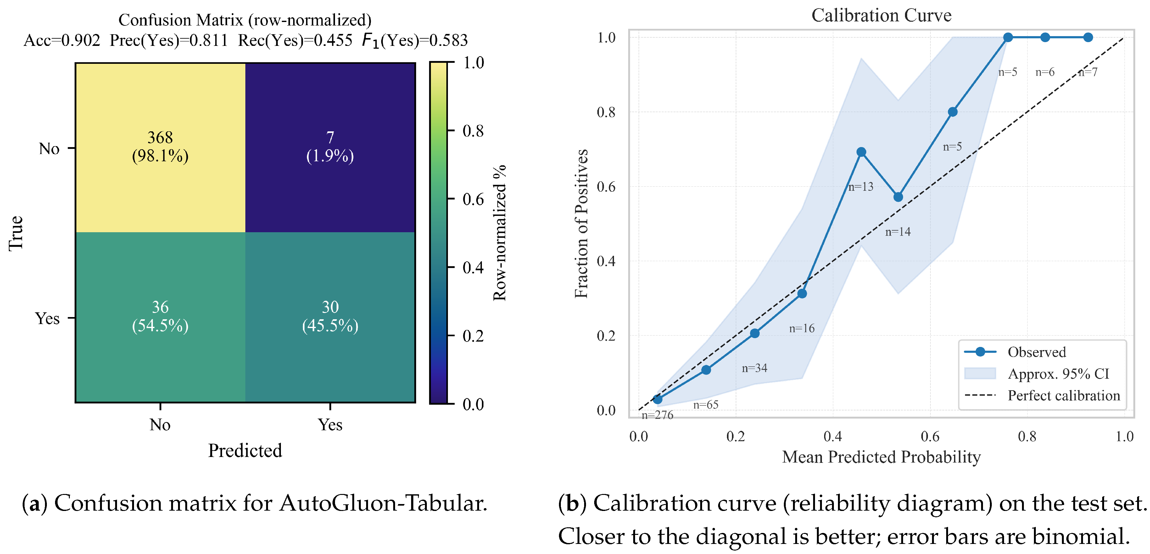
To ground the effect, Figure 4(a) reports the AutoGluon-Tabular confusion matrix. Of 375 non-attrition employees, 368 are true negatives and 7 false positives; among 66 attrition cases, 30 are true positives and 36 false negatives. Thus accuracy , precision (attrition) , and recall (attrition) . High precision means few false alarms; moderate recall suggests threshold tuning can trade precision for more coverage of at-risk employees.
Figure 4.
Confusion matrix and calibration of AutoGluon-Tabular, side by side for compact comparison.
Figure 4.
Confusion matrix and calibration of AutoGluon-Tabular, side by side for compact comparison.
3.2. Fairness Analysis
We assess gender fairness under equal opportunity (groupwise TPR on the attrition class). For AutoGluon-Tabular, female TPR is 42.1% and male TPR is 50.0%, so the TPR gap is about 8%. This indicates slightly higher sensitivity for males. Because base rates differ slightly by gender, we track both groupwise TPRs and the gap; we do not impose fairness constraints in training. False positive rates are low (about 2–3%) and similar across genders.
3.3. Reliability and Calibration
Figure 4(b) shows a reliability diagram for AutoGluon-Tabular. Predictions are well calibrated at low probabilities, with mild underestimation in the mid-range. The Brier score is , better than logistic regression (). A constant forecaster at the base rate (15%) would achieve . We did not apply post-hoc calibration (e.g., Platt scaling or isotonic regression) to keep the evaluation on raw outputs.
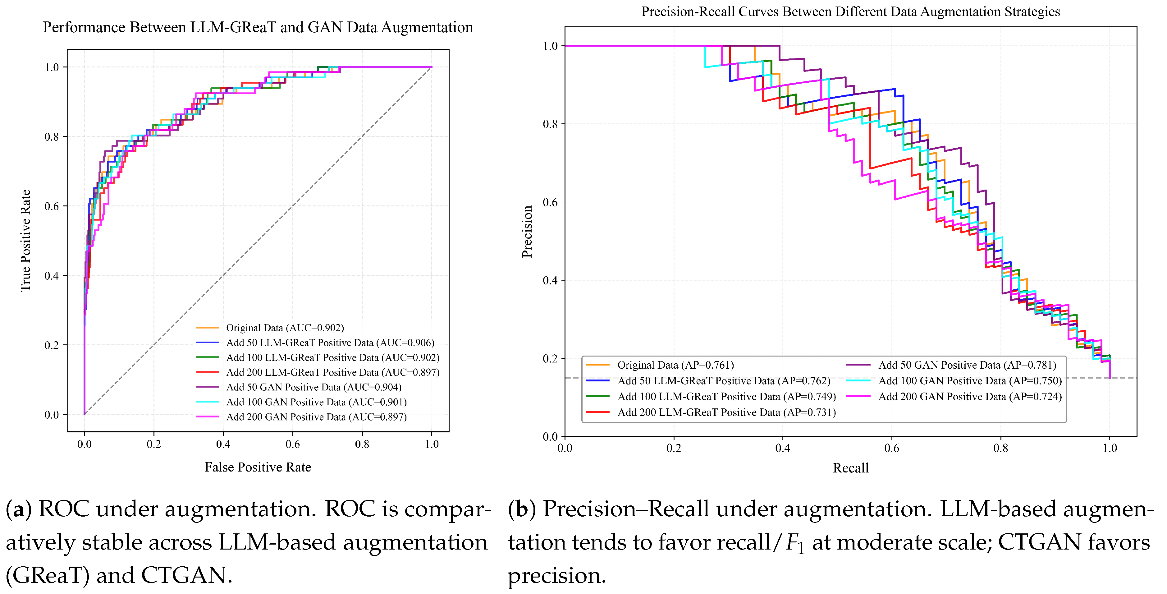
We next compare LLM-based augmentation (GReaT) to CTGAN. Figure 5 contrasts three training sets per model (none, , synthetic “Yes”). For AutoGluon-Tabular, AP declines slightly as synthetic size grows; TabTransformer drops more. The likely cause is small distributional shifts from synthetic samples. CTGAN shows higher precision at small scales but lower recall. Overall, ROC is stable across scales, whereas PR exposes method-specific trade-offs.
Figure 5.
ROC and PR with synthetic augmentation (LLM-based augmentation via GReaT vs. CTGAN). ROC varies little with scale, while PR reveals trade-offs: for AutoGluon, AP decreases slightly with ( ); TabTransformer drops more (). CTGAN tends to raise precision at small scales at a cost to recall. Over-augmentation degrades PR, highlighting the need for quality control.
Figure 5.
ROC and PR with synthetic augmentation (LLM-based augmentation via GReaT vs. CTGAN). ROC varies little with scale, while PR reveals trade-offs: for AutoGluon, AP decreases slightly with ( ); TabTransformer drops more (). CTGAN tends to raise precision at small scales at a cost to recall. Over-augmentation degrades PR, highlighting the need for quality control.
3.4. Interpretability of Model Predictions
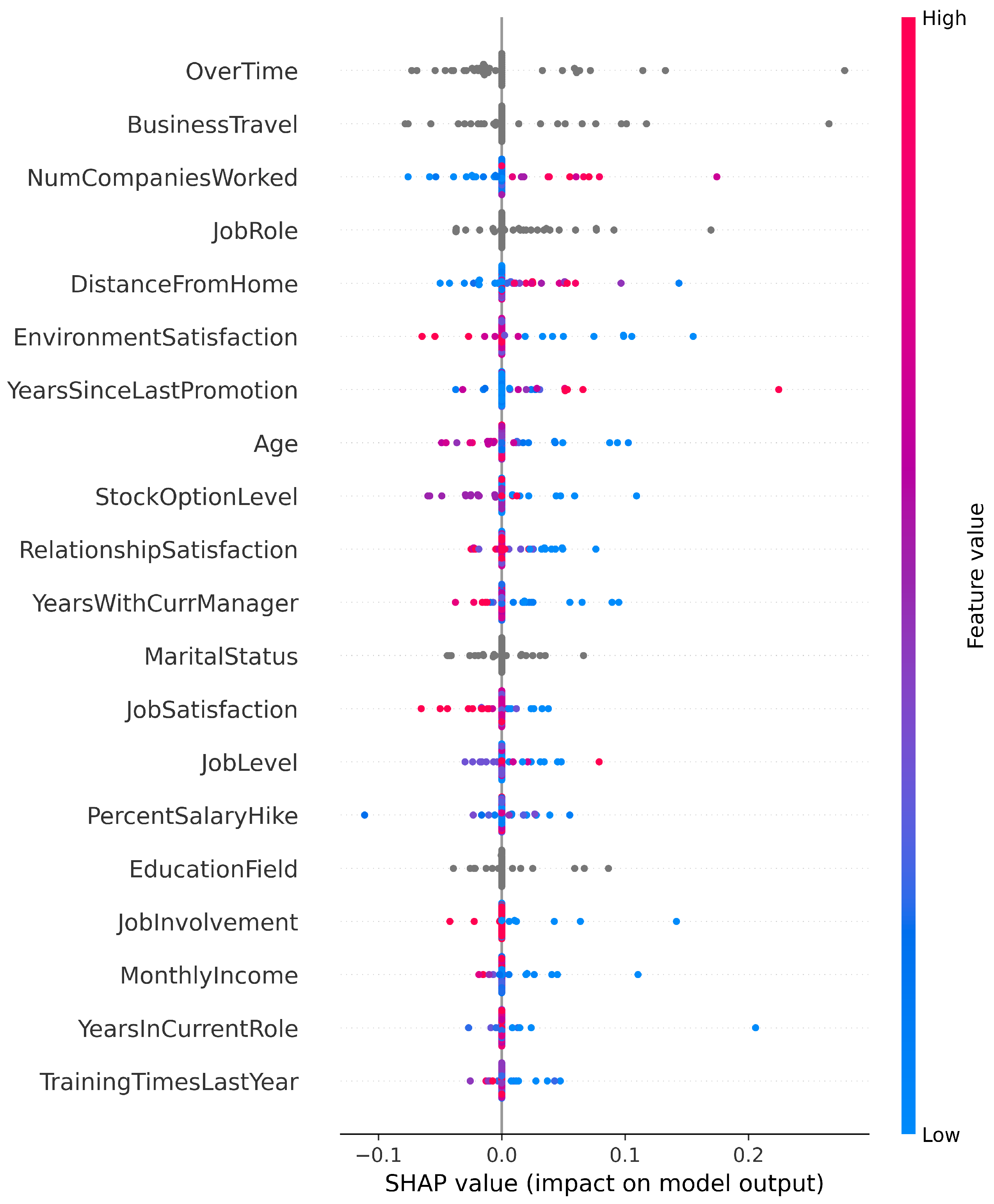
To ensure transparency, we examine SHAP for AutoGluon-Tabular (Figure 6). OverTime, BusinessTravel, NumCompaniesWorked, JobRole, and DistanceFromHome have the largest effects. Signs align with HR intuition: more overtime, frequent travel, many past employers, certain roles, and long commutes raise risk; satisfaction and tenure dynamics moderate it. Sensitive attributes (e.g., gender) are not top drivers, which lowers fairness concerns and yields actionable levers.
3.5. GReaT vs. GAN: Practical Comparison
GReaT fine-tuning is straightforward and stable, yielding diverse, plausible samples. CTGAN is powerful but requires careful tuning and can produce near-duplicates or constraint violations that need filtering. Multiple LLM sampling runs are more consistent than GAN runs in practice. For reuse, LLM-based augmentation adapts with light prompting or brief fine-tuning; GANs typically need full retraining.
Table 2 shows two patterns. First, both families peak near synthetic samples (LLM: higher /recall; GAN: balanced /MCC). Larger scales () degrade PR metrics, suggesting distributional noise. Second, LLM-based augmentation tilts toward recall/ (broader coverage), while GAN-based augmentation tilts toward precision (fewer alerts but more misses). The choice depends on whether the HR program prioritizes coverage or intervention efficiency.
Figure 6.
SHAP summary for AutoGluon-Tabular. Features are ordered by mean absolute SHAP. Red points indicate higher feature values; blue points indicate lower values. Key features such as OverTime, BusinessTravel, NumCompaniesWorked, JobRole, and DistanceFromHome dominate attributions.
Figure 6.
SHAP summary for AutoGluon-Tabular. Features are ordered by mean absolute SHAP. Red points indicate higher feature values; blue points indicate lower values. Key features such as OverTime, BusinessTravel, NumCompaniesWorked, JobRole, and DistanceFromHome dominate attributions.
The omnibus DeLong test was significant(), indicating heterogeneous ROC–AUCs across models (Table 3). AutoGluon achieved the highest AUC (), losely followed by TabTransformer () and Logistic Regression (). Random Forest () and XGBoost () were lower, while KNN underperformed ().
Post-hoc pairwise DeLong tests (Table 4) showed that AutoGluon outperformed XGBoost, Random Forest, and KNN after Holm correction (). Differences between AutoGluon and Logistic Regression or TabTransformer were not significant after correction. Consistently, KNN was significantly worse than XGBoost, Random Forest, Logistic Regression, and TabTransformer (all Holm ). Several uncorrected p-values near (e.g., XGBoost vs. Logistic Regression/TabTransformer; Random Forest vs. Logistic Regression/TabTransformer) did not survive Holm FWER control, though they were borderline under BH-FDR.
The omnibus DeLong test did not reject equality of AUCs (), indicating no detectable AUC differences among augmentation settings (Table 5). Numerically, the AUCs were tightly clustered around 0.90: LLM+50, GAN+50 , LLM+100 , GAN+100 , and both LLM+200 and GAN+200 . In post-hoc pairwise tests (Table 6), no contrast remained significant after Holm correction. Practically, AutoGluon’s ROC discrimination appears stable across augmentation type and size in this data; to assess rare-event sensitivity, we recommend complementing ROC-AUC with PR-AUC/recall comparisons (e.g., paired bootstrap for AP).
4. Discussion
Our findings show that LLM-based augmentation (GReaT) can meaningfully support decision-centric attrition prediction, with the most consistent benefit being an increase in recall (sensitivity) for the minority class. Across experiments, augmented models caught more true positives—i.e., more at-risk employees—than their non-augmented counterparts. In decision contexts where missed leavers (false negatives) cost more than false alarms, this gain in recall is practically valuable. For example, recall improvements from to among 100 potential leavers translate into preventing 10 extra departures, which can yield large savings relative to the incremental costs of false positives.
Selective Metric Gains. It is important to note that this recall improvement does not extend uniformly to all metrics. Discrimination measures such as ROC-AUC remained essentially unchanged or slightly lower with LLM augmentation, and Average Precision (AP) showed no significant uplift. Statistical tests (DeLong’s test) confirm that observed AUC differences between augmented and non-augmented models are not statistically significant. This indicates that the main performance shift is selective: recall improves while AUC and AP remain stable. The underlying mechanism is intuitive: oversampling with synthetic positives shifts the classifier’s boundary to capture more positives, raising sensitivity but at the cost of a modest increase in false positives. Precision therefore does not improve proportionally, explaining why composite metrics like AP and AUC stay flat.
Cost–Benefit Implications. From a managerial perspective, the asymmetry between false negatives and false positives provides the rationale for prioritizing recall. Industry evidence estimates replacement costs at roughly – annual salary and pegs U.S. annual voluntary turnover losses near $1T.2 If recall gains prevent 10 departures at $60k each (saving $600k), while five extra false positives each cost $5k in intervention ($25k), the net benefit is about $575k. This stylized example illustrates why recall-oriented augmentation strategies can deliver strong ROI despite modest precision trade-offs.
Model Interpretability and Feature Insights. SHAP analyses confirm that both augmented and baseline models identify similar, intuitive drivers (OverTime, BusinessTravel, NumCompaniesWorked, satisfaction and tenure signals). The consistency of feature importance across augmented and non-augmented runs supports face validity and stakeholder trust, ensuring that recall gains do not come at the expense of interpretability.
Comparison to Other Augmentation Methods. Relative to CTGAN, GReaT is operationally simpler (no adversarial dynamics), supports fully conditional sampling, and produced diverse yet plausible records. CTGAN remained competitive but required careful tuning and occasionally generated near-duplicates at small scales. Both methods show characteristic trade-offs: GAN-based augmentation leaned toward higher precision at small scales, while LLM-based augmentation favored recall/. Over-augmentation hurt both, highlighting the need to tune augmentation rather than maximize it.
Precision–Recall Balance and Filtering. Our results align with a known generative trade-off: greater synthetic diversity expands recall of the data manifold but can lower fidelity (precision)[48]. To mitigate this, we applied critic-based filtering—scoring LLM samples with a trained CTGAN discriminator and retaining only high-quality records. Unfiltered LLM outputs were not evaluated in this study, so our conclusions pertain specifically to the filtered augmentation pipeline. This step mirrors techniques like discriminator rejection sampling and helped stabilize performance.
Practical Limitations. LLM-based augmentation adds compute costs (fine-tuning and sampling) and requires disciplined validation (schema checks, deduplication) to avoid artifacts. Benefits are model- and dataset-dependent: deeper models like TabTransformer were more sensitive to heavy augmentation. We therefore recommend case-by-case evaluation, tuning augmentation size and weighting, and considering hybrid approaches (e.g., mixing in synthetic negatives).
Managerial Takeaways. When budgets are tight and false alarms must be minimized, precision-leaning augmentation (e.g., small-scale GAN-based) may be preferable. When the priority is preventing as many departures as possible, recall-leaning augmentation (moderate, quality-controlled LLM-based) is attractive. In all cases, pair augmentation with fairness monitoring and SHAP explanations so decisions remain equitable and actionable. Overall, repurposing LLMs for tabular augmentation offers HR analytics teams a pragmatic, recall-oriented tool—complementary to AutoML/ensembles—that merits deployment under leakage-aware protocols.
5. Conclusions
This study shows that LLM-based augmentation in the style of GReaT [4] can raise minority-class recall for employee attrition under severe imbalance. By adding realistic synthetic “leaver” records, augmented training flagged more at-risk employees, with modest precision trade-offs and generally preserved calibration. A leakage-aware protocol ensured that gains did not arise from target leakage, supporting the robustness of the findings.
Our contributions are fourfold. (i) We operationalize a leakage-aware modeling and evaluation framework that yields fair estimates on small, imbalanced tabular data. (ii) We assess fairness and interpretability—via equal-opportunity style group metrics [29] and SHAP explanations [30]—to verify that augmented predictions remain equitable and transparent. (iii) We benchmark classical, boosted-tree, transformer, and AutoML ensembles, and show that LLM-augmented training improves minority recall and balanced accuracy over non-augmented baselines. (iv) We analyze augmentation scale and identify a practical operating region: recall gains plateau beyond moderate levels, and over-augmentation can degrade PR metrics. Augmentation should therefore be tuned rather than maximized. Together, these results integrate modern generative AI into an end-to-end, decision-oriented HR analytics pipeline.
From a decision-support perspective, higher recall means surfacing more would-be leavers for timely intervention—valuable in settings where false negatives are costlier than false positives. Notably, these gains were achieved while preserving interpretability (feature attributions aligned with domain knowledge via SHAP) and while keeping subgroup TPR gaps small (consistent with equal-opportunity fairness). Looking ahead, the same LLM-driven tabular augmentation can extend to other rare-event domains (e.g., churn, fraud, or risk) and can pair with prescriptive policies (thresholds and action rules) to move from prediction to intervention. Targeted conditioning during generation (e.g., subgroup-aware augmentation) and quality control (e.g., critic-based filtering) are promising next steps to further improve utility and fairness.
Overall, this work shows how cutting-edge generative AI can be woven into established analytics workflows to support managerial decisions. In line with DSAM’s mission, our leakage-aware, interpretable, and fairness-conscious augmentation helps bridge advanced methods and practical HR deployment, offering a scalable path to more informed, equitable, and cost-effective retention strategies.
Author Contributions
Conceptualization, Liao Weiquan and Jiayangmei Xu; methodology, Liao Weiquan; software, Liao Weiquan and Jiayangmei Xu; validation, Liao Weiquan and Jiayangmei Xu; formal analysis, Liao Weiquan; investigation, Liao Weiquan and Jiayangmei Xu; resources, Liao Weiquan; data curation, Jiayangmei Xu; writing—original draft preparation, Liao Weiquan; writing—review and editing, Liao Weiquan and Ekaterina A. Panova; visualization, Liao Weiquan; supervision, Ekaterina A. Panova; project administration, Ekaterina A. Panova. All authors have read and agreed to the published version of the manuscript.
Funding
This research received no external funding.
Institutional Review Board Statement
Not applicable.
Informed Consent Statement
Not applicable.
Data Availability Statement
The IBM HR Analytics Employee Attrition dataset used in this study is publicly available at https://www.kaggle.com/datasets/pavansubhasht/ibm-hr-analytics-attrition-dataset. No new data were created or analyzed in this study beyond synthetic augmentations derived from the original dataset.
Acknowledgments
The authors thank the anonymous reviewers for their valuable feedback and suggestions, which helped improve the quality of this manuscript. We also acknowledge the IBM HR Analytics Employee Attrition dataset provided via Kaggle and the open-source software communities (e.g., AutoGluon, PyTorch) that supported our experiments. During the preparation of this study, the authors used OpenAI ChatGPT (GPT-5, 2025) solely for generating auxiliary Python code (e.g., data preprocessing, visualization scripts). The authors have reviewed and validated all code outputs and take full responsibility for the results and interpretations presented in this publication.
Conflicts of Interest
The authors declare no conflicts of interest.
Abbreviations
The following abbreviations are used in this manuscript:
| MDPI | Multidisciplinary Digital Publishing Institute |
| DOAJ | Directory of open access journals |
| TLA | Three letter acronym |
| LD | Linear dichroism |
References
- Harter, J. & Adkins, A. This Fixable Problem Costs U.S. Businesses $1 Trillion. Gallup Workplace (2019). Available online: https://www.gallup.com/workplace/247391/fixable-problem-costs-businesses-trillion.aspx (accessed on 31 July 2025).
- Qi, Z.; Wang, Y.; Kong, D.; Wang, M. Applying oversampling before cross-validation will lead to high bias in small data sets. Scientific Reports 2024, 14, 62585. [Google Scholar] [CrossRef]
- NeurIPS Paper Checklist Guidelines (accessed 31 July 2025). Available online: https://neurips.cc/public/guides/PaperChecklist.
- Borisov, V.; Seßler, K.; Leemann, T.; Pawelczyk, M.; Kasneci, G. Language Models are Realistic Tabular Data Generators. In International Conference on Learning Representations ICLR. 2023. Available online: https://openreview.net/forum?id=HyeaUS1hXZ (accessed on 31 July 2025).
- Scikit Learn: Preprocessing data. 2025. https://scikit-learn.org/stable/modules/preprocessing.html (accessed on 21 August 2025).
- Scikit Learn: OneHotEncoder. 2025. https://scikit-learn.org/stable/modules/generated/sklearn.preprocessing.OneHotEncoder.html (accessed on 21 August 2025).
- Scikit Learn: train_test_split. 2025. https://scikit-learn.org/stable/modules/generated/sklearn.model_selection.train_test_split.html (accessed on 21 August 2025).
- Scikit Learn: StratifiedKFold. 2025. https://scikit-learn.org/stable/modules/generated/sklearn.model_selection.StratifiedKFold.html (accessed on 21 August 2025).
- Scikit Learn: LogisticRegression. 2025. https://scikit-learn.org/stable/modules/generated/sklearn.linear_model.LogisticRegression.html (accessed on 21 August 2025).
- Ian, T. Jolliffe; Jorge Cadima.Principal component analysis: a review and recent developments. Phil. Trans. R. Soc. A. 2016, 374. [Google Scholar] [CrossRef]
- Scikit Learn: PCA. 2025. https://scikit-learn.org/stable/modules/generated/sklearn.decomposition.PCA.html (accessed on 21 August 2025).
- Laurens van der Maaten; Geoffrey Hinton. Visualizing Data using t-SNE. Journal of Machine Learning Research 2008, 9(86), 2579–2605. http://jmlr.org/papers/v9/vandermaaten08a.html.
- Scikit Learn: TSNE. 2025. https://scikit-learn.org/stable/modules/generated/sklearn.manifold.TSNE.html (accessed on 21 August 2025).
- Samaneh Azadi; Catherine Olsson; Trevor Darrell; Ian J. Goodfellow; Augustus Odena. Discriminator Rejection Sampling. In Proceedings of the 7th International Conference on Learning Representations, ICLR. 2018. https://openreview.net/forum?id=S1GkToR5tm.
- Salimans, Tim; Goodfellow, Ian; Zaremba, Wojciech; Cheung, Vicki; Radford, Alec; Chen, Xi. Improved techniques for training GANs. In Proceedings of the 30th International Conference on Neural Information Processing Systems NeurIPS. 2016. [CrossRef]
- YData-Synthetic: Synthesize tabular data. 2025. https://docs.synthetic.ydata.ai/1.3/synthetic_data/single_table/ctgan_example/ (accessed on 21 August 2025).
- AutoGluon. TabularPredictor.fit. 2025 https://auto.gluon.ai/dev/api/autogluon.tabular.TabularPredictor.fit.html (accessed on 21 August 2025).
- Scikit Learn. BalancedRandomForestClassifier. 2025. https://imbalanced-learn.org/stable/references/generated/imblearn.ensemble.BalancedRandomForestClassifier.html (accessed on 21 August 2025).
- Scikit Learn. roc_auc_score. 2025. https://scikit-learn.org/stable/modules/generated/sklearn.metrics.roc_auc_score.html (accessed on 21 August 2025).
- Chao Chen; Andy Liaw; Leo Breiman. Using Random Forest to Learn Imbalanced Data. University of California, Berkeley, 2004. https://statistics.berkeley.edu/sites/default/files/tech-reports/666.pdf.
- XGBoost. XGBoost Parameters. 2025. https://xgboost.readthedocs.io/en/stable/parameter.html (accessed on 21 August 2025).
- Tianqi Chen; Carlos Guestrin. XGBoost: A Scalable Tree Boosting System. In Proceedings of the 22nd ACM SIGKDD International Conference on Knowledge Discovery and Data MiningKDD’16. 2016. [CrossRef]
- Scikit Learn. GridSearchCV. 2025. https://scikit-learn.org/stable/modules/generated/sklearn.model_selection.GridSearchCV.html (accessed on 21 August 2025).
- Scikit Learn. StratifiedKFold. 2025. https://scikit-learn.org/stable/modules/generated/sklearn.model_selection.StratifiedKFold.html (accessed on 21 August 2025.
- Xu, Lei; Skoularidou, Maria; Cuesta-Infante, Alfredo; Veeramachaneni, Kalyan. Modeling Tabular Data using Conditional GAN. In Proceedings of the 33rd International Conference on Neural Information Processing Systems NeurIPS. 2019. [CrossRef]
- Austin A. Barr; Robert Rozman; Eddie Guo. Generative adversarial networks vs large language models: a comparative study on synthetic tabular data generation. Available online: https://arxiv.org/abs/2502.14523 (accessed on 19 August 2025).
- Xin Huang; Ashish Khetan; Milan Cvitkovic; Zohar Karnin. TabTransformer: Tabular Data Modeling Using Contextual Embeddings. Available online: https://arxiv.org/abs/2012.06678 (accessed on 19 October 2025).
- Decision Science and Analytics for Management (DSAM) Topic Page. MDPI. Available online: https://www.mdpi.com/topics/9D1436TTND (accessed on 31 July 2025).
- Hardt, M.; Price, E.; Srebro, N. Equality of Opportunity in Supervised Learning. In Proceedings of the 30th International Conference on Neural Information Processing Systems,NeurIPS 2016; Barcelona, Spain, 2016.
- Lundberg, S.M.; Lee, S.-I. A Unified Approach to Interpreting Model Predictions. In Proceedings of the 31th International Conference on Neural Information Processing Systems,NeurIPS 2017; Long Beach, California, USA, 2017.
- IBM Watson Analytics. IBM HR Analytics Employee Attrition & Performance Dataset; 2015. Available online: https://www.kaggle.com/datasets/pavansubhasht/ibm-hr-analytics-attrition-dataset (accessed on 31July 2025).
- Edward J. Hu; Yelong Shen; Phillip Wallis; Zeyuan Allen-Zhu; Yuanzhi Li; Shean Wang; Lu Wang; Weizhu Chen. LoRA: Low-Rank Adaptation of Large Language Models. In The Tenth International Conference on Learning Representations, ICLR, 2022.
- Erickson, N.; Mueller, J.; Zhang, H.; et al. AutoGluon-Tabular: Robust and Accurate AutoML for Structured Data. arXiv 2020, arXiv:2003.06505.
- Zhiqiang; Tang; Haoyang Fang; Su Zhou; Taojiannan Yang; Zihan Zhong; Tony Hu; Katrin Kirchhoff; George Karypis. AutoGluon-Multimodal (AutoMM): Supercharging Multimodal AutoML with Foundation Models. In The International Conference on Automated Machine Learning AutoML, 2024.
- Huang, H.; Zhang, H.; Li, K.; et al. TabTransformer: Tabular Data Modeling Using Contextual Embeddings. arXiv 2020, arXiv:2012.06678.
- Feldman, Michael; Friedler, Sorelle A.; Moeller, John; Scheidegger, Carlos; Venkatasubramanian, Suresh. Certifying and removing disparate impact. In Proceedings of the 21th ACM SIGKDD International Conference on Knowledge Discovery and Data Mining; Sydney, NSW, Australia, 2015.
- Katy Molodianovitch; David Faraggi; Benjamin Reiser. Comparing the Areas Under Two Correlated ROC Curves: Parametric and Non-Parametric Approaches. Biometrics 2006, 48(5), 745-757. [CrossRef]
- Saito, T.; Rehmsmeier, M. The Precision-Recall Plot Is More Informative than the ROC Plot When Evaluating Binary Classifiers on Imbalanced Datasets. PLOS ONE 2015, 10(3), 1-21. [CrossRef]
- Peter A. Flach, Meelis Kull. Precision-Recall-Gain curves: PR analysis done right. In Proceedings of the 29th International Conference on Neural Information Processing Systems NeurIPS; Montreal, Canada. [CrossRef]
- BRIER, G. W. (1950). VERIFICATION OF FORECASTS EXPRESSED IN TERMS OF PROBABILITY. Monthly Weather Review 2023 78(1), 1-3. [CrossRef]
- Telmo Silva Filho; Hao Song; Miquel Perello-Nieto; Raul Santos-Rodriguez; Meelis Kull; Peter Flach. Classifier calibration: a survey on how to assess and improve predicted class probabilities. Mach Learn 2023, 112, 3211–3260. [CrossRef]
- Davis, J.; Goadrich, M. The Relationship Between Precision-Recall and ROC Curves. In Proceedings of the 23rd International Conference on Machine learning ICML; 2006. Pittsburgh, PA, USA. [CrossRef]
- Chawla, N.V.; Bowyer, K.W.; Hall, L.O.; Kegelmeyer, W.P. SMOTE: Synthetic Minority Over-sampling Technique. Journal of Artificial Intelligence ResearchJ. Artif. Int. Res. 2002, 16, 321–357. [Google Scholar] [CrossRef]
- Goodfellow, Ian J.; Pouget-Abadie, Jean; Mirza, Mehdi; Xu, Bing; Warde-Farley, David; Ozair, Sherjil; Courville, Aaron; Bengio, Yoshua. In Proceedings of the 28th International Conference on Neural Information Processing Systems NeurIPS; New York, NY, USA. [CrossRef]
- Ryan D. Turner; Jane Hung; Yunus Saatci; Jason Yosinski. Metropolis-Hastings Generative Adversarial Networks. In Proceedings of the 36rd International Conference on Machine learning ICML; 2019. Pittsburgh, PA, USA. https://proceedings.mlr.press/v97/turner19a/turner19a.pdf.
- Guo, Chuan; Pleiss, Geoff; Sun, Yu; Weinberger, Kilian Q.. On calibration of modern neural networks. In Proceedings of the 34rd International Conference on Machine learning ICML; 2017. Sydney, NSW, Australia. [CrossRef]
- Xin Ding; Yongwei Wang; Z. Jane Wang; William J. Welch. Efficient subsampling of realistic images from GANs conditional on a class or a continuous variable. Neurocomputing 2023, 517, 188-200. [CrossRef]
- Sajjadi, Mehdi S. M.; Bachem, Olivier; Lucic, Mario; Bousquet, Olivier; Gelly, Sylvain. Assessing generative models via precision and recall. In Proceedings of the 32nd International Conference on Neural Information Processing Systems NeurIPS; 2018. [CrossRef]
| 1 | At the GAN optimum , so . |
| 2 | Leaders and scarce roles tend to sit near the upper end. |
Figure 1.
Leakage-Aware LLM Augmentation Framework
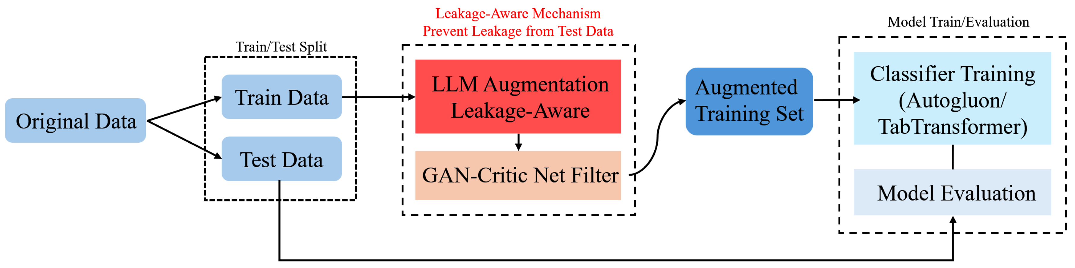
Figure 2.
Visualization of the training data in (left) PCA and (right) t-SNE space. Purple points denote non-attrition and yellow points denote attrition. The considerable overlap highlights the challenge.
Figure 2.
Visualization of the training data in (left) PCA and (right) t-SNE space. Purple points denote non-attrition and yellow points denote attrition. The considerable overlap highlights the challenge.
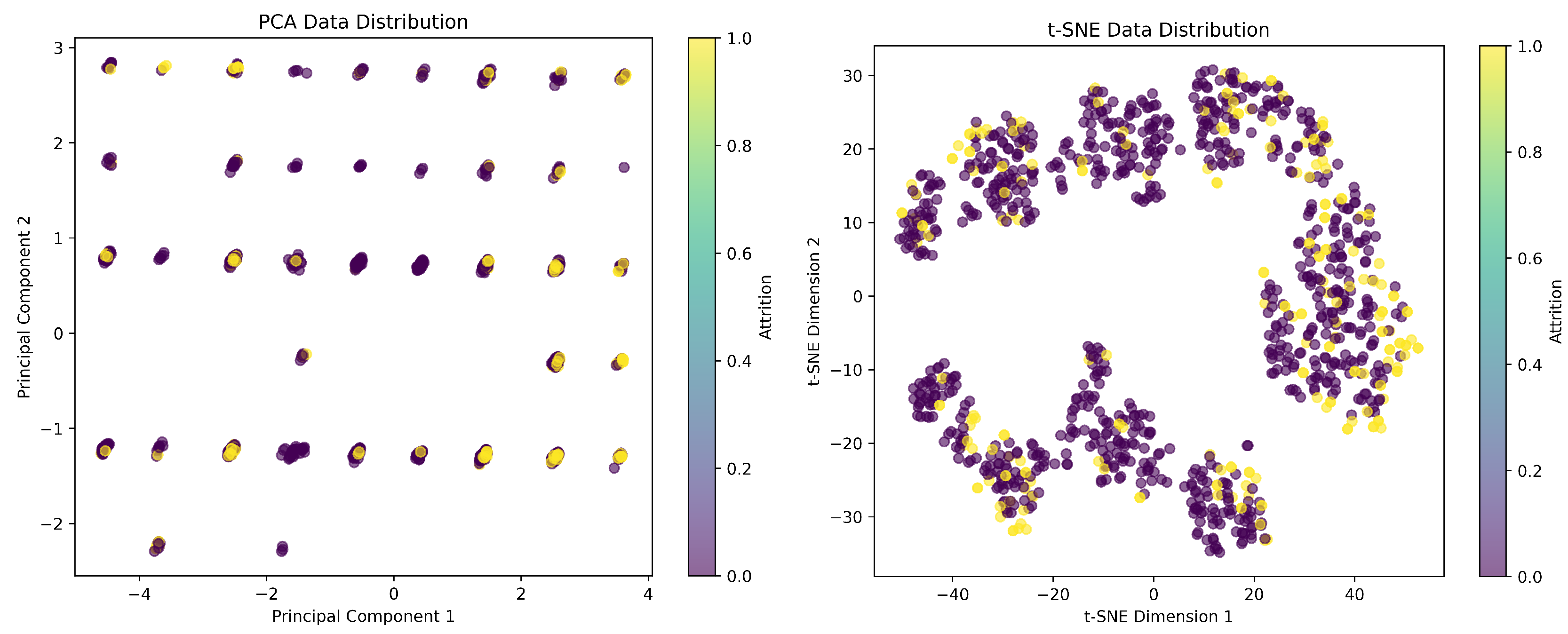

Table 1.
Overall performance (mean over 20 repeated stratified splits). AutoGluon-Tabular ranks first on ROC-AUC and AP, followed by TabTransformer; tree-based and linear baselines are lower.
Table 1.
Overall performance (mean over 20 repeated stratified splits). AutoGluon-Tabular ranks first on ROC-AUC and AP, followed by TabTransformer; tree-based and linear baselines are lower.
| Model | Performance Evaluation | ||||
|---|---|---|---|---|---|
| ROC AUC | Precision | Recall | Avg Precision | ||
| AutoGluon | 0.902 | 0.900 | 0.409 | 0.562 | 0.761 |
| TabTransformer | 0.899 | 0.827 | 0.363 | 0.505 | 0.704 |
| Logistic Regression | 0.894 | 0.833 | 0.303 | 0.444 | 0.698 |
| Random Forest | 0.852 | 0.800 | 0.181 | 0.296 | 0.568 |
| XGBoost | 0.841 | 0.800 | 0.363 | 0.500 | 0.629 |
Table 2.
LLM- vs. GAN-based augmentation with AutoGluon. Metrics include ROC-AUC, Accuracy, Precision, Recall, , Balanced Accuracy, and MCC. Results suggest an optimal region near samples, with degradation at .
Table 2.
LLM- vs. GAN-based augmentation with AutoGluon. Metrics include ROC-AUC, Accuracy, Precision, Recall, , Balanced Accuracy, and MCC. Results suggest an optimal region near samples, with degradation at .
| Method | Aug. Size | ROC AUC | Acc | Precision | Recall | MCC | |
|---|---|---|---|---|---|---|---|
| LLM-based | 50 | 0.906 | 0.907 | 0.857 | 0.455 | 0.594 | 0.582 |
| 100 | 0.902 | 0.914 | 0.833 | 0.530 | 0.648 | 0.622 | |
| 200 | 0.897 | 0.900 | 0.824 | 0.424 | 0.560 | 0.546 | |
| GAN-based | 50 | 0.904 | 0.912 | 0.966 | 0.424 | 0.589 | 0.607 |
| 100 | 0.901 | 0.912 | 0.865 | 0.485 | 0.621 | 0.607 | |
| 200 | 0.897 | 0.909 | 0.842 | 0.485 | 0.615 | 0.596 |
Table 3.
ROC–AUC with DeLong 95% confidence intervals on the common test set. Omnibus DeLong/Wald test: , .
Table 3.
ROC–AUC with DeLong 95% confidence intervals on the common test set. Omnibus DeLong/Wald test: , .
| Model | AUC | 95% CI (DeLong) |
|---|---|---|
| AutoGluon | ||
| TabTransformer | ||
| Logistic Regression | ||
| Random Forest | ||
| XGBoost | ||
| KNN |
Table 4.
Pairwise DeLong post-hoc comparisons on the common test set. AUC = AUC(Model i) − AUC(Model j). controls FWER; controls FDR. Entries with are in bold.
Table 4.
Pairwise DeLong post-hoc comparisons on the common test set. AUC = AUC(Model i) − AUC(Model j). controls FWER; controls FDR. Entries with are in bold.
| Model i | Model j | AUC | z | p (raw) | ||
|---|---|---|---|---|---|---|
| AutoGluon | XGBoost | |||||
| AutoGluon | Random Forest | |||||
| AutoGluon | KNN | |||||
| AutoGluon | Logistic Regression | |||||
| AutoGluon | TabTransformer | |||||
| XGBoost | Random Forest | |||||
| XGBoost | KNN | |||||
| XGBoost | Logistic Regression | |||||
| XGBoost | TabTransformer | |||||
| Random Forest | KNN | |||||
| Random Forest | Logistic Regression | |||||
| Random Forest | TabTransformer | |||||
| KNN | Logistic Regression | |||||
| KNN | TabTransformer | |||||
| Logistic Regression | TabTransformer |
Table 5.
ROC–AUC with DeLong 95% CIs on the common test set across augmentation settings. Omnibus DeLong/Wald: , .
Table 5.
ROC–AUC with DeLong 95% CIs on the common test set across augmentation settings. Omnibus DeLong/Wald: , .
| Variant | AUC | 95% CI (DeLong) |
|---|---|---|
| LLM+50 | 0.906 | [0.864, 0.947] |
| GAN+50 | 0.904 | [0.861, 0.948] |
| LLM+100 | 0.902 | [0.860, 0.944] |
| GAN+100 | 0.901 | [0.858, 0.944] |
| LLM+200 | 0.897 | [0.856, 0.939] |
| GAN+200 | 0.897 | [0.856, 0.939] |
Table 6.
Pairwise DeLong comparisons among augmentation variants on the common test set. AUC = AUC(Variant i) − AUC(Variant j). Holm controls FWER; BH controls FDR. No contrast remains significant after Holm correction.
Table 6.
Pairwise DeLong comparisons among augmentation variants on the common test set. AUC = AUC(Variant i) − AUC(Variant j). Holm controls FWER; BH controls FDR. No contrast remains significant after Holm correction.
| Variant i | Variant j | AUC | z | p (raw) | ||
|---|---|---|---|---|---|---|
| LLM+50 | LLM+100 | |||||
| LLM+50 | LLM+200 | 9.451e-01 | ||||
| LLM+50 | GAN+50 | 9.738e-01 | ||||
| LLM+50 | GAN+100 | 9.451e-01 | ||||
| LLM+50 | GAN+200 | 9.451e-01 | ||||
| LLM+100 | LLM+200 | 9.451e-01 | ||||
| LLM+100 | GAN+50 | 9.738e-01 | ||||
| LLM+100 | GAN+100 | 9.808e-01 | ||||
| LLM+100 | GAN+200 | 9.451e-01 | ||||
| LLM+200 | GAN+50 | 9.451e-01 | ||||
| LLM+200 | GAN+100 | 9.738e-01 | ||||
| LLM+200 | GAN+200 | 9.808e-01 | ||||
| GAN+50 | GAN+100 | 9.451e-01 | ||||
| GAN+50 | GAN+200 | 9.451e-01 | ||||
| GAN+100 | GAN+200 | 9.451e-01 |
Disclaimer/Publisher’s Note: The statements, opinions and data contained in all publications are solely those of the individual author(s) and contributor(s) and not of MDPI and/or the editor(s). MDPI and/or the editor(s) disclaim responsibility for any injury to people or property resulting from any ideas, methods, instructions or products referred to in the content. |
© 2025 by the authors. Licensee MDPI, Basel, Switzerland. This article is an open access article distributed under the terms and conditions of the Creative Commons Attribution (CC BY) license (http://creativecommons.org/licenses/by/4.0/).
Copyright: This open access article is published under a Creative Commons CC BY 4.0 license, which permit the free download, distribution, and reuse, provided that the author and preprint are cited in any reuse.


