Submitted:
10 September 2025
Posted:
11 September 2025
You are already at the latest version
Abstract
(1) Background: Accurate demand forecasting is essential for supply chain management, guiding operational planning, decision-making, and resource allocation. Evaluating classical statistical and AI approaches is crucial for selecting suitable forecasting techniques. (2) Methods: This case study assessed five approaches—classical statistical algorithms, machine learning models, and a hybrid method—using consumption data from a retail chain. Performance was measured by predictive accuracy (sMAPE), training and testing latency, memory usage, and storage requirements. (3) Results: XGBoost achieved the best balance, with low predictive error (sMAPE = 1.03%), minimal latency (79.3 ms), and moderate memory usage (359.58 MiB). SARIMAX and Holt-Winters remained competitive, providing robust, interpretable, and efficient predictions. LSTM showed higher computational demands (867.52 MiB) and lower accuracy (sMAPE = 3.7), while the Holt-Winters plus XGBoost hybrid did not outperform individual methods (sMAPE = 1.36). Classical algorithms produced optimistic forecasts, supporting make-to-stock strategies, whereas AI models were more conservative, aligned with a following-demand approach. (4) Conclusions: Model selection should consider predictive accuracy, operational costs, product characteristics, and organizational strategies. Results are dataset-specific and cannot be generalized. Limitations include the absence of exogenous variables. Traditional statistical methods remain competitive, interpretable, and efficient against AI approaches in structured demand forecasting.
Keywords:
demand forecasting
; time series
; statistical models
; artificial intelligence
; comparative analysis
1. Introduction
Demand forecasting plays a central role in supply chain management, guiding operational strategies, managerial decisions, and corporate planning [1]. According to [2], it involves identifying patterns in historical behavior data to anticipate future outcomes, and may also include analyzing factors that shape such behavior, enabling trend projection over time.
In today’s competitive landscape, suppliers must anticipate market needs and align production capacity accordingly. Ref. [3] highlight that higher productivity requires replacing experience- and intuition-based approaches with more analytical and precise methods. Consequently, demand forecasting provides critical data to support informed decision-making.
Recent years have seen a significant increase in studies focused on time series-based demand forecasting [4]. A time series can be understood as a dataset of observations collected sequentially over time, either at regular or irregular intervals, providing a chronological record of events [5]. The growing complexity of operational environments and market volatility has driven the development of increasingly sophisticated forecasting models. In that regard, machine learning and deep neural network methods have gained rapid attention due to their strong performance in contexts characterized by nonlinear and complex patterns [6,7,8,9].
This trend has been accompanied by a growing number of studies comparing statistical techniques and machine learning algorithms across criteria such as accuracy, scalability, and computational complexity [10]. In parallel, research has increasingly explored hybrid models that combine multiple approaches to enhance predictive performance [11].
Although the literature on demand forecasting has expanded considerably, most studies still emphasize predictive performance. Operational aspects, such as processing latency and memory consumption, have received less attention, despite being critical for real-world deployment [10,12]. By evaluating both accuracy and computational costs, researchers can achieve a more comprehensive understanding of model suitability in practical scenarios.
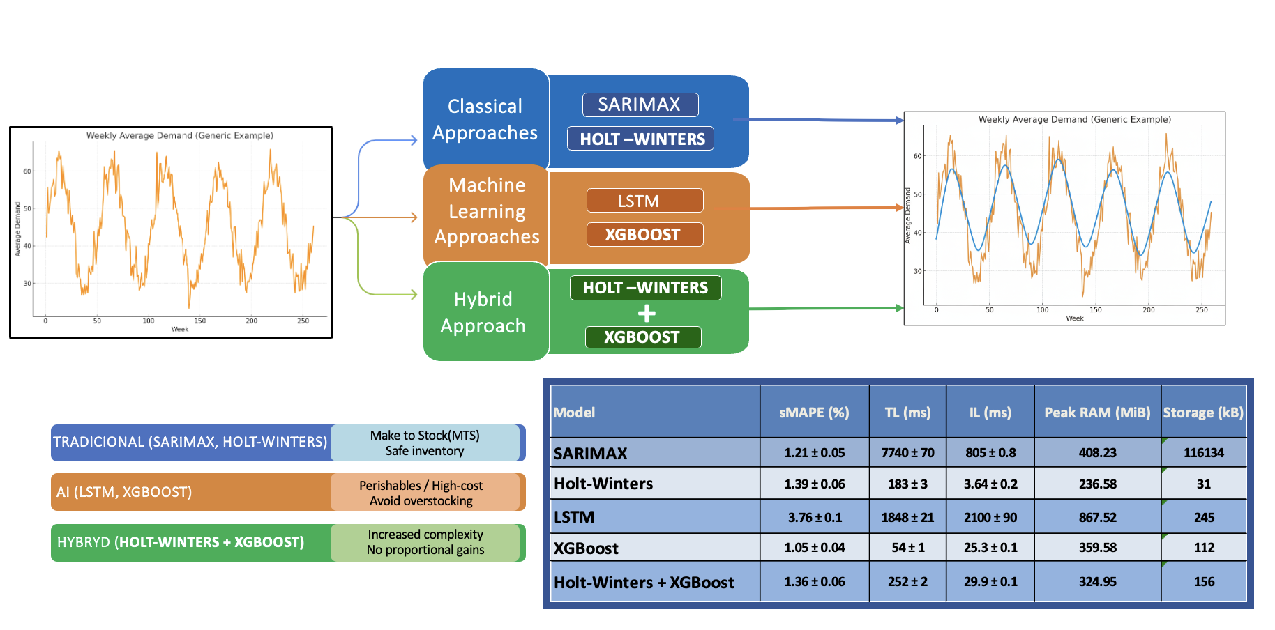
This case study analyzes a range of demand forecasting models, including classical statistical methods, machine learning algorithms, and a hybrid approach. The evaluation was conducted using a retail chain dataset, applying metrics such as predictive accuracy (sMAPE), processing latency, and memory consumption. The objective is to compare the performance of traditional models against recent machine learning and hybrid schemes within this practical context.
By integrating predictive performance with operational considerations, this study provides practical insights into the selection of forecasting techniques. The contribution lies in demonstrating under which conditions, for this particular case, traditional models can remain competitive, and in identifying which types of products or production strategies may benefit from either statistical, AI-based, or hybrid approaches.
2. Materials and Methods
This applied research with a quantitative approach uses open data from a Kaggle dataset [13], containing daily demand records for 50 different products across 10 stores over a five-year period from a retail chain. For simplification purposes, the demand of all products was aggregated weekly using the mean, resulting in a single time series representative of the overall demand. Analyses were conducted using Python with the support of the libraries pandas [14], numpy [15], matplotlib [16], seaborn [17], statsmodels [18], scikit-learn [19], and tensorflow [20].
A total of five distinct models were employed, selected to represent classical statistical algorithms, AI-based algorithms, and hybrid methods, following common practices identified in the literature for problems of this nature [7,21,22,23,24]. The performance of each model was evaluated using the symmetric mean absolute percentage error (sMAPE), training latency, prediction latency, model file size, and peak RAM usage. This approach aims to provide a comprehensive view on the trade-offs of each strategy in terms of predictive performance and computational costs.
2.1. Data Preprocessing
A logarithmic transformation was initially applied to adjust the data scale and improve visualization. The time series was then decomposed to explore its individual components: trend, seasonality, and residuals. Stationarity was formally assessed using the augmented Dickey-Fuller (ADF) test with Ȧutocorrelation (ACF) and partial autocorrelation (PACF) plots were also inspected as diagnostic tools. To verify stationarity, a first-order weekly differencing was applied, which reduced trend components and stabilized the mean of the series. Finally, z-score standardization was applied to the data to ensure that AI models are not affected by differences in feature scale [25,26]. The last year of data, corresponding to 52 weeks, was reserved for testing the fitted models. Forecast accuracy was further evaluated through 1,000 resamplings of rolling time windows with variable lengths.
2.2. Modeling
This subsection aims to describe the selected algorithms and the parameters employed, in order to ensure transparency and replicability of the conducted experiments.
2.2.1. SARIMAX
The Seasonal AutoRegressive Integrated Moving Average with eXogenous variables (SARIMAX) model extends the seasonal ARIMA framework by incorporating external variables (X) to enhance forecasting accuracy and predictive performance [27]. In this study, SARIMAX was selected for its ability to handle seasonality and reduce errors, even when input and output series have similar lengths and directions [28]. The model’s order parameters (p, d, q) and seasonal order parameters (P, D, Q, s) were determined through empirical testing and analysis of the time series behavior, including the examination of ACF and PACF plots. In this context, p represents the number of autoregressive (AR) terms, d is the number of differences applied, and q is the number of moving average (MA) terms, while P is the seasonal AR term, D is the seasonal differencing, Q is the seasonal MA term, and s denotes the seasonal periodicity [29]. The full implementation is presented as follows:
where B is the backshift operator, and are the AR and MA polynomials, and are the seasonal AR and MA polynomials, is the random error, and is the regression with exogenous variables X. Thus, , , and were defined based on the experiments and observations conducted.
2.2.2. Holt-Winters
The Holt-Winters exponential smoothing method was selected for its simplicity and its ability to effectively model data with both trend and seasonal variations [30]. This forecasting approach applies exponential smoothing based on the results of the previous period’s forecast and incorporates a parameter to account for seasonal patterns, capturing repeated variations around the intercept and trend [31]. Accordingly, additive trend and seasonality were adopted, and the seasonal period was again set to 52 weeks (1 year), as observed in the data behavior. The forecast for k steps ahead at time i is calculated as:
where represents the estimated level at time i, is the estimated trend at the same time, denotes the estimated seasonal component considering the seasonal period m, and k is the number of steps ahead for the forecast. This formulation allows the model to simultaneously capture the current level, trend, and seasonality, providing accurate predictions for future periods [32].
2.2.3. LSTM
The Long Short-Term Memory (LSTM) algorithm, widely used in natural language processing and time series forecasting [33,34], consists of a memory cell () that stores information, updated by three special gates: the input gate (), the forget gate (recurrent loop with weight ), and the output gate () [35]. These gates, together with the activation functions (S) and the weight connections (), provide a mechanism to address the vanishing gradient problem observed in recurrent neural networks (RNNs) [36]. Figure 1 illustrates the components described within this algorithm.
LSTM networks are particularly useful in time-series problems for their ability to capture long-term dependencies in sequential and multivariate time-series data, and to directly map input sequences to multi-step output forecasts [37]. Thus, the implemented model consists of two stacked LSTM layers, each with 32 neurons, followed by a dense layer with 64 neurons using the Rectified Linear Unit (ReLU) as the activation function. To improve generalization and prevent overfitting [38], two Dropout layers with a rate of 0.1 were incorporated: one placed between the two LSTM layers and another between the second LSTM layer and the dense layer. The output layer contains a number of neurons equal to the number of steps to be predicted, providing flexibility while maintaining prediction stability [23]. The Adaptive Moment Estimation (ADAM) was employed as the optimizer, and the cost function was calculated using the mean absolute percentage error (MAPE). Again, the previous 52 periods were considered for the prediction. Training was stopped after 27 epochs due to the application of the early stopping technique, which monitors the validation error. The training was interrupted when no improvement greater than 0.001 was observed in the errors over 5 consecutive epochs, thus preventing model overfitting.
2.2.4. XGBoost
The Extreme Gradient Boosting (XGBoost) algorithm is widely used in various data mining tasks and combines multiple weak classifiers into a single strong classifier in a linear manner and performs a second-order Taylor expansion of the cost function to extract richer information [5]. In this study, XGBoost was chosen for its flexibility in modeling complex and nonlinear relationships, robustness to outliers, and ability to automatically capture feature interactions [39]. The regularized objective function minimized by XGBoost is expressed as:
where l is the loss function, and are the actual and predicted values for observation i at iteration , is the newly added tree, and is a regularization term that penalizes the complexity of . Using a second-order Taylor expansion, the objective can be approximated as:
where and are the first and second derivatives of the loss function with respect to the previous prediction. In the present implementation, regression relies on the last 52 periods immediately preceding the target value. Hyperparameters were optimized via grid search to enhance performance: the fraction of columns per tree (colsample_bytree) was set to 0.8, the learning rate (learning_rate) to 0.2, the maximum tree depth (max_depth) to 3, the number of estimators (n_estimators) to 50, and the fraction of samples per tree (subsample) to 0.8.
2.2.5. Hybrid Model
For the hybrid time series model, aspects of traditional trend and seasonality modeling were combined with machine learning methods to capture more complex patterns in the forecast residuals. Initially, the Holt-Winters model with additive trend and seasonality is applied to predict the main demand series. The residuals are then analyzed separately. To model them, lagged features are created, transforming the residual series into a supervised learning problem. An XGBoost model is subsequently trained on these lags to predict future errors. The final forecasts are obtained by adding the predictions from the Holt-Winters model to the residual predictions from XGBoost. This approach aims to leverage the strengths of both strategies, combining the ability to capture linear and seasonal patterns with the capacity to model nonlinear relationships in the errors [31,40,41,42]. For the hybrid implementation, the same parameters as in the individual Holt-Winters and XGBoost models were maintained.
2.3. Experimental procedure
Model performance was evaluated using metrics that capture both predictive accuracy and computational costs. Predictive accuracy was measured using sMAPE, defined as:
where is the actual value at time t, is the predicted value, and n is the total number of observations. Lower sMAPE values indicate better predictive performance. While MAPE is highly sensitive to small actual values (), where even minor absolute deviations can produce disproportionately large percentage errors [43], sMAPE provides a more balanced measure, reducing the impact of small denominators and offering a more reliable assessment of predictive accuracy in time series data [44,45].
The reliability of sMAPE was assessed using a random window resampling procedure. For each iteration, all observations preceding a randomly selected point in the test set were added to the training set, and a prediction window of random length was used to compute the metric.
Computational costs were quantified via model latencies, measured in milliseconds for training (TL) and inference (IL), as well as model file size (kB) and peak RAM usage (MiB), reporting the maximum observed RAM.
Margins of error (ME) for sMAPE, LT, and LI were computed as:
where is the standard deviation across iterations N and z corresponds to the desired confidence level.
The experiments were conducted on a machine equipped with an Intel® Core™ i5-10210U CPU @ 1.60 GHz, 8 GB RAM, running Windows 10 (64-bit). No dedicated GPU was used, and all computations relied solely on the CPU. All metrics, including sMAPE, latency, and peak RAM, were obtained based on 1000 iterations, providing a robust assessment of model performance and variability. A confidence interval of 0.05 was adopted in all evaluations.
3. Results
The five years of product demand were initially inspected visually to identify possible intuitive trends and seasonal patterns in the data. The complete time series is presented in Figure 2.
The preliminary inspection revealed the presence of a slight upward trend over time combined with a well-defined annual seasonality, with demand peaks in the middle of the year and low periods at the beginning and end. This behavior remained consistent throughout the entire available history and is better illustrated through its decomposition into trend, seasonality, and residuals, as shown in Figure 3.
Using the additive model for decomposition, the positively sloped trend line confirms the initial observation of a temporal increase in demand, possibly reflecting the organic growth of the organization. Additionally, the seasonality is emphasized by its cyclical behavior observed over the years, indicating that demand is considerably sensitive to different seasons. The residuals are very close to zero, suggesting a relatively homogeneous distribution with few outliers, although slight signs of heteroscedasticity are present, considering the variation in variance amplitude over time. A more in-depth assessment of data stationarity is illustrated in Figure 4, through the analysis of the ACF and PACF tests.
Despite the p-value of 0.04 obtained from the Augmented Dickey-Fuller (ADF) test, some evidence suggests that the series is not fully stationary. These indicators include the slow decay of the ACF, a pronounced peak at the first lag in the PACF followed by a sharp drop, as well as the presence of trend and seasonality observed visually.
After applying a weekly differencing, the signs of non-stationarity were significantly reduced, and the ADF p-value dropped to 0.0001, increasing the confidence that the transformed series is stationary.
With these adjustments, and ensuring that the model assumptions were properly addressed, the selected algorithms were trained and validated using data from the most recent year available. The performance comparison of each model is presented in Figure 5, where the actual demand is highlighted in blue and the predicted values are shown in red.
The observation of the results indicates that all tested models demonstrated good predictive capability, generating curves that closely follow the actual data. In general, classical statistical models — SARIMAX and Holt-Winters — tended to be more optimistic, often projecting values higher than the original data. In contrast, AI-based models — XGBoost and LSTM — were more conservative, frequently predicting values below the actual observations. The hybrid model — Holt-Winters + XGBoost — closely followed the optimistic trend of the classical models, often producing predictions above the original values.
Table 1 summarizes the results obtained in terms of sMAPE, computational latency, and memory usage for each evaluated model, providing additional guidance for selecting the most appropriate strategy for the specific context under consideration.
XGBoost was the model with the best overall performance, achieving the lowest predictive error (sMAPE = 1.03%) and presenting very low training latency (54 ms) and testing latency (25.3 ms), in addition to a relatively moderate memory consumption (359.58 MiB). Its ability to balance accuracy and speed, even though it was not originally designed for time series tasks, highlights the potential of the model in production environments that require high responsiveness with predictive reliability.
SARIMAX, the second-best in terms of error (sMAPE = 1.21%), reinforces its relevance as an interpretable statistical model. However, its training latency (7.74 s) was significantly higher, as well as memory usage (408.23 MiB) and storage demand (116 MB), which may compromise its application in scenarios requiring scalability or real-time operation. Nevertheless, its ability to incorporate exogenous variables and provide greater transparency in the results can make it attractive in analytical or strategic contexts.
Holt-Winters maintained its appeal due to its computational efficiency, with the lowest training time (183 ms), testing time of only 3.64 ms, and the smallest file size among all models (31 kB). Although it showed a slightly higher error (sMAPE = 1.39%), its overall efficiency positions it as an excellent option for systems that require fast updates and low resource consumption, even with a small loss in accuracy.
In contrast, LSTM presented the worst accuracy (sMAPE = 3.70%) and high computational costs: training time of 19.1 s, testing time of 2.1 s, and peak memory usage of 867.52 MiB. Although it was the model with the greatest theoretical capacity to capture nonlinear patterns, its practical results did not translate into a competitive advantage in this application, limiting its feasibility for productive use.
Finally, the Holt-Winters + XGBoost combination did not outperform the individual models. Despite achieving a relatively low error (sMAPE = 1.36%), the hybrid approach resulted in higher latencies (252 ms for training and 29.9 ms for testing) and increased computational complexity without significant performance gains compared to XGBoost alone. Therefore, the combination strategy was not justified given the additional implementation costs.
4. Discussion
Therefore, the choice of the most appropriate model depends not only on predictive accuracy but also on the computational costs associated with training, inference, and memory usage, which are decisive factors in real-world applications. In this study, statistical models displayed a tendency to overestimate demand, while artificial intelligence models were more conservative, often underestimating it. These forecasting profiles suggest different potential uses: overestimation may be advantageous in make-to-stock (MTS) strategies [46], where anticipating higher demand can help mitigate the risk of stockouts, whereas underestimation may be preferable in demand-following contexts, such as perishable goods, high unit-value products, or items with significant storage and logistics costs, where avoiding excess inventory is critical. Although the computational costs observed in this study are relatively low, the results provide useful indications for larger-scale applications, in which scalability and resource efficiency are likely to become decisive for the feasibility of the solution.
The results of this case study corroborate previous findings, showing that traditional statistical methods can remain competitive with artificial intelligence models in time series with relatively structured patterns. Ref. [21] demonstrated that, although AI models may achieve slightly better performance, accuracy gains are not always statistically significant compared to established solutions, such as linear regression or ARIMA. Ref. [22,47] emphasize the robustness, computational efficiency, and interpretability of traditional methods, in contrast with the higher cost and complexity of implementing deep learning approaches. Even with the growing use of neural networks and hybrid models in high-uncertainty contexts [7,23,48], classical methods continue to offer viable solutions, particularly when computational costs and inference speed are important. Overall, the choice between traditional and AI methods should consider the operational context, as lower predictive error does not always imply a practical advantage. By addressing these complementary dimensions, this research contributes to the development of a framework that can support managers and decision-makers in selecting the most appropriate forecasting model according to specific business contexts.
5. Conclusions
This study analyzed a range of demand forecasting models, including classical statistical methods, machine learning algorithms, and hybrid approaches, evaluating both predictive performance and operational metrics such as training and testing latency, memory usage, and storage requirements. XGBoost achieved the best overall balance, with low sMAPE, minimal latency, and moderate memory usage, making it suitable for responsive production environments. Classical models remained competitive, with SARIMAX providing strong predictive accuracy at higher computational cost and Holt-Winters offering operational efficiency despite slightly higher error. LSTM showed lower accuracy and high computational demands, while the Holt-Winters plus XGBoost hybrid did not outperform the individual models. Overall, the study fulfilled its objective by providing practical insights for choosing forecasting techniques aligned with product characteristics and organizational production strategies. The results obtained on a low-cost machine without a dedicated GPU suggest that the proposed approach may be feasible in real-world scenarios with limited computational resources.
An important limitation of this research is the use of a single dataset from a retail chain, which may restrict the generalizability of the findings to other industries or time series with different demand patterns. Additionally, the analysis did not include exogenous variables, which could affect model performance.
Future studies could replicate this evaluation across multiple sectors and datasets to assess the robustness and scalability of the models. Investigating hybrid and ensemble approaches under varying demand scenarios, incorporating exogenous variables, and considering the computational cost relative to predictive gains would provide further guidance for operational deployment. These directions would help clarify under which conditions AI or classical models offer practical advantages and support more informed decision-making in supply chain management.
Abbreviations
The following abbreviations are used in this manuscript:
| ACF | Autocorrelation function |
| ADAM | Adaptive Moment Estimation |
| ADF | Augmented Dickey-Fuller test |
| AI | Artificial Intelligence |
| ARIMA | AutoRegressive Integrated Moving Average |
| IL | Inference latency |
| kB | Kilobytes |
| LSTM | Long Short-Term Memory |
| MAPE | Mean absolute percentage error |
| ME | Margins of error |
| MiB | Mebibytes |
| MS | Milliseconds |
| MTS | Make-to-stock |
| PACF | Partial autocorrelation function |
| RAM | Random Access Memory |
| ReLU | Rectified Linear Unit |
| SARIMAX | Seasonal AutoRegressive Integrated Moving Average with eXogenous variables |
| sMAPE | Symmetric mean absolute percentage error |
| TL | Training latency |
| XGBoost | Extreme Gradient Boosting |
Author Contributions
Conceptualization, R.A.C.; methodology, R.A.C.; software, R.A.C.; validation, R.A.C.; formal analysis, R.A.C. and E.C.M.S.; investigation, R.A.C.; resources, R.A.C.; data curation, R.A.C.; writing—original draft preparation, R.A.C. and E.C.M.S.; writing—review and editing, R.A.C., E.C.M.S., S.C.M.B., M.C.G. and M.G.M.P.; visualization, R.A.C. and E.C.M.S.; supervision, E.C.M.S., S.C.M.B., M.C.G. and M.G.M.P.; project administration, E.C.M.S.; funding acquisition, S.C.M.B., M.C.G. and M.G.M.P. All authors have read and agreed to the published version of the manuscript.
Funding
This research received no external funding.
Data Availability Statement
Restrictions apply to the availability of these data. Data were obtained from Kaggle and are available at https://www.kaggle.com/competitions/demand-forecasting-kernels-only with the permission of Kaggle.
Acknowledgments
The authors would like to thank the University of Brasilia (UnB) and the Fundação de Apoio à Pesquisa do Distrito Federal (FAPDF) for their institutional support during the development of this research.
Conflicts of Interest
The authors declare no conflicts of interest.
Abbreviations
The following abbreviations are used in this manuscript:
References
- Kumar, R. A Comprehensive Study on Demand Forecasting Methods and Algorithms for Retail Industries. J. Univ. Shanghai Sci. Technol 2021, 23, 409–420. [Google Scholar]
- Ackermann, A.E.; Sellitto, M.A. Métodos de previsão de demanda: uma revisão da literatura. Innovar 2022, 32, 83–99. [Google Scholar] [CrossRef]
- Tanizaki, T.; Hoshino, T.; Shimmura, T.; Takenaka, T. Restaurants store management based on demand forecasting. Procedia CIRP 2020, 88, 580–583. [Google Scholar] [CrossRef]
- Arunkumar, O.; Divya, D. Deep learning techniques for demand forecasting: review and future research opportunities. Information Resources Management Journal (IRMJ) 2022, 35, 1–24. [Google Scholar] [CrossRef]
- Zhang, L.; Bian, W.; Qu, W.; Tuo, L.; Wang, Y. Time series forecast of sales volume based on XGBoost. In Proceedings of the Journal of Physics: Conference Series. IOP Publishing, Vol. 1873; 2021; p. 012067. [Google Scholar]
- Hahn, Y.; Langer, T.; Meyes, R.; Meisen, T. Time series dataset survey for forecasting with deep learning. Forecasting 2023, 5, 315–335. [Google Scholar] [CrossRef]
- Feizabadi, J. Machine learning demand forecasting and supply chain performance. International Journal of Logistics Research and Applications 2022, 25, 119–142. [Google Scholar] [CrossRef]
- Bernal Lara, I.I.; Lorenzo Diaz, R.J.; Sánchez Galván, M.d.l.Á.; Robles García, J.; Badaoui, M.; Romero Romero, D.; Moreno Flores, R.A. Probabilistic Demand Forecasting in the Southeast Region of the Mexican Power System Using Machine Learning Methods. Forecasting 2025, 7, 39. [Google Scholar] [CrossRef]
- Fourkiotis, K.P.; Tsadiras, A. Applying machine learning and statistical forecasting methods for enhancing pharmaceutical sales predictions. Forecasting 2024, 6, 170–186. [Google Scholar] [CrossRef]
- Schmid, L.; Roidl, M.; Kirchheim, A.; Pauly, M. Comparing statistical and machine learning methods for time series forecasting in data-driven logistics—A simulation study. Entropy 2024, 27, 25. [Google Scholar] [CrossRef] [PubMed]
- Wang, X.; Hyndman, R.J.; Li, F.; Kang, Y. Forecast combinations: An over 50-year review. International Journal of Forecasting 2023, 39, 1518–1547. [Google Scholar] [CrossRef]
- Makridakis, S.; Spiliotis, E.; Assimakopoulos, V.; Semenoglou, A.A.; Mulder, G.; Nikolopoulos, K. Statistical, machine learning and deep learning forecasting methods: Comparisons and ways forward. Journal of the Operational Research Society 2023, 74, 840–859. [Google Scholar] [CrossRef]
- Inversion. Store Item Demand Forecasting Challenge. https://kaggle.com/competitions/demand-forecasting-kernels-only, 2018. Kaggle.
- McKinney, W.; et al. Data structures for statistical computing in Python. scipy 2010, 445, 51–56. [Google Scholar]
- Oliphant, T.E. Python for scientific computing. Computing in science & engineering 2007, 9, 10–20. [Google Scholar]
- Hunter, J.D. Matplotlib: A 2D graphics environment. Computing in science & engineering 2007, 9, 90–95. [Google Scholar]
- Waskom, M.L. Seaborn: statistical data visualization. Journal of open source software 2021, 6, 3021. [Google Scholar] [CrossRef]
- Seabold, S.; Perktold, J.; et al. Statsmodels: econometric and statistical modeling with python. SciPy 2010, 7, 92–96. [Google Scholar]
- Pedregosa, F.; Varoquaux, G.; Gramfort, A.; Michel, V.; Thirion, B.; Grisel, O.; Blondel, M.; Prettenhofer, P.; Weiss, R.; Dubourg, V.; et al. Scikit-learn: Machine learning in Python. the Journal of machine Learning research 2011, 12, 2825–2830. [Google Scholar]
- Abadi, M.; Barham, P.; Chen, J.; Chen, Z.; Davis, A.; Dean, J.; Devin, M.; Ghemawat, S.; Irving, G.; Isard, M.; et al. {TensorFlow}: a system for {Large-Scale} machine learning. In Proceedings of the 12th USENIX symposium on operating systems design and implementation (OSDI 16); 2016; pp. 265–283. [Google Scholar]
- Carbonneau, R.; Laframboise, K.; Vahidov, R. Application of machine learning techniques for supply chain demand forecasting. European journal of operational research 2008, 184, 1140–1154. [Google Scholar] [CrossRef]
- Makridakis, S.; Spiliotis, E.; Assimakopoulos, V. Statistical and Machine Learning forecasting methods: Concerns and ways forward. PloS one 2018, 13, e0194889. [Google Scholar] [CrossRef]
- Abbasimehr, H.; Shabani, M.; Yousefi, M. An optimized model using LSTM network for demand forecasting. Computers & industrial engineering 2020, 143, 106435. [Google Scholar]
- Islam, B.u.; Ahmed, S.F. Short-term electrical load demand forecasting based on LSTM and RNN deep neural networks. Mathematical Problems in Engineering 2022, 2022, 2316474. [Google Scholar] [CrossRef]
- Giri, C.; Chen, Y. Deep learning for demand forecasting in the fashion and apparel retail industry. Forecasting 2022, 4, 565–581. [Google Scholar] [CrossRef]
- Cobo, M.; Menéndez Fernández-Miranda, P.; Bastarrika, G.; Lloret Iglesias, L. Enhancing radiomics and Deep Learning systems through the standardization of medical imaging workflows. Scientific data 2023, 10, 732. [Google Scholar] [CrossRef] [PubMed]
- Manigandan, P.; Alam, M.S.; Alharthi, M.; Khan, U.; Alagirisamy, K.; Pachiyappan, D.; Rehman, A. Forecasting natural gas production and consumption in United States-evidence from SARIMA and SARIMAX models. Energies 2021, 14, 6021. [Google Scholar] [CrossRef]
- Alharbi, F.R.; Csala, D. A seasonal autoregressive integrated moving average with exogenous factors (SARIMAX) forecasting model-based time series approach. Inventions 2022, 7, 94. [Google Scholar] [CrossRef]
- Tarsitano, A.; Amerise, I.L. Short-term load forecasting using a two-stage sarimax model. Energy 2017, 133, 108–114. [Google Scholar] [CrossRef]
- Kochetkova, I.; Kushchazli, A.; Burtseva, S.; Gorshenin, A. Short-term mobile network traffic forecasting using seasonal ARIMA and holt-winters models. Future Internet 2023, 15, 290. [Google Scholar] [CrossRef]
- Djakaria, I.; Saleh, S. Covid-19 forecast using Holt-Winters exponential smoothing. In Proceedings of the Journal of physics: conference series. IOP Publishing, Vol. 1882; 2021; p. 012033. [Google Scholar]
- Sawalha, S.; Al-Naymat, G. An Adaptive Holt–Winters Model for Seasonal Forecasting of Internet of Things (IoT) Data Streams. IoT 2025, 6, 39. [Google Scholar] [CrossRef]
- Sundermeyer, M.; Schlüter, R.; Ney, H. Lstm neural networks for language modeling. In Proceedings of the Interspeech, Vol. 2012; pp. 194–197. [Google Scholar]
- Sundermeyer, M.; Ney, H.; Schlüter, R. From feedforward to recurrent LSTM neural networks for language modeling. IEEE/ACM transactions on audio, speech, and language processing 2015, 23, 517–529. [Google Scholar] [CrossRef]
- Cao, J.; Li, Z.; Li, J. Financial time series forecasting model based on CEEMDAN and LSTM. Physica A: Statistical mechanics and its applications 2019, 519, 127–139. [Google Scholar] [CrossRef]
- Hochreiter, S.; Schmidhuber, J. Long short-term memory. Neural computation 1997, 9, 1735–1780. [Google Scholar] [CrossRef]
- Ghanbari, R.; Borna, K. Multivariate time-series prediction using LSTM neural networks. In Proceedings of the 2021 26th International Computer Conference, Computer Society of Iran (CSICC). IEEE; 2021; pp. 1–5. [Google Scholar]
- Xiao, F. Time series forecasting with stacked long short-term memory networks. arXiv preprint arXiv:2011.00697, arXiv:2011.00697 2020.
- Mishra, P.; Al Khatib, A.M.G.; Yadav, S.; Ray, S.; Lama, A.; Kumari, B.; Sharma, D.; Yadav, R. Modeling and forecasting rainfall patterns in India: a time series analysis with XGBoost algorithm. Environmental Earth Sciences 2024, 83, 163. [Google Scholar] [CrossRef]
- Cawood, P.; Van Zyl, T. Evaluating state-of-the-art, forecasting ensembles and meta-learning strategies for model fusion. Forecasting 2022, 4, 732–751. [Google Scholar] [CrossRef]
- Chen, T.; Guestrin, C. system. In Proceedings of the Proceedings of the 22nd acm sigkdd international conference on knowledge discovery and data mining, 2016, pp.
- He, Y.; Tao, L.; Zhang, Z. Enhancing decomposition-based hybrid models for forecasting multivariate and multi-source time series by federated transfer learning. Expert Systems with Applications, 1277. [Google Scholar]
- Makridakis, S. Accuracy measures: theoretical and practical concerns. International journal of forecasting 1993, 9, 527–529. [Google Scholar] [CrossRef]
- Vancsura, L.; Tatay, T.; Bareith, T. Navigating AI-Driven Financial Forecasting: A Systematic Review of Current Status and Critical Research Gaps. Forecasting 2025, 7, 36. [Google Scholar] [CrossRef]
- St-Aubin, P.; Agard, B. Precision and reliability of forecasts performance metrics. Forecasting 2022, 4, 882–903. [Google Scholar] [CrossRef]
- Heizer, J.H.; Render, B. Principles of operations management; Pearson Educación, 2004.
- Hyndman, R.J.; Athanasopoulos, G. Forecasting: principles and practice; OTexts, 2018.
- Yazici, I.; Beyca, O.F.; Delen, D. Deep-learning-based short-term electricity load forecasting: A real case application. Engineering Applications of Artificial Intelligence 2022, 109, 104645. [Google Scholar] [CrossRef]
Figure 1.
LSTM cell diagram showing gates, cell state, outputs, and recurrent connections [36].
Figure 1.
LSTM cell diagram showing gates, cell state, outputs, and recurrent connections [36].
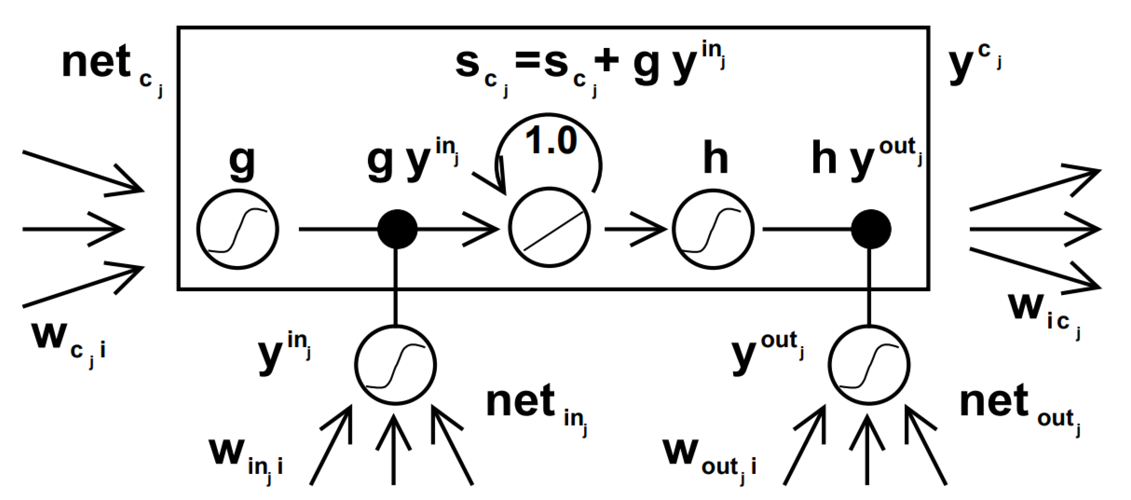
Figure 2.
Weekly average product demand.
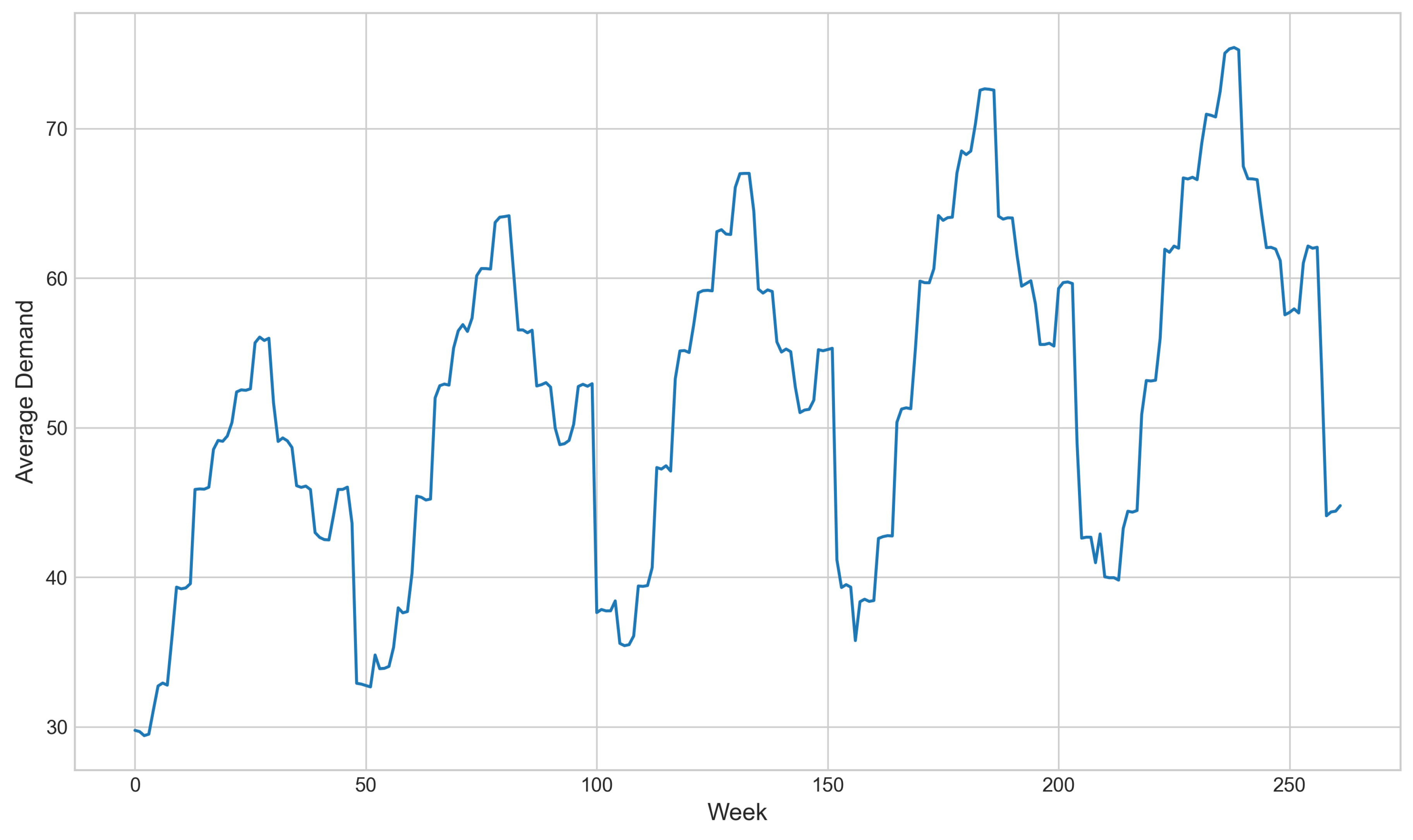
Figure 3.
Demand decomposition.
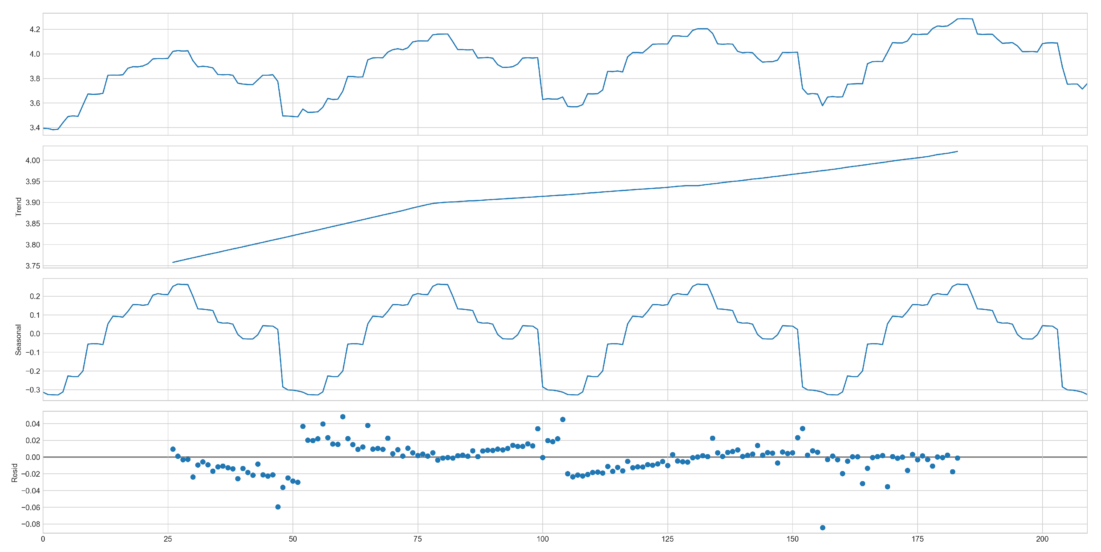
Figure 4.
ACF and PACF tests.
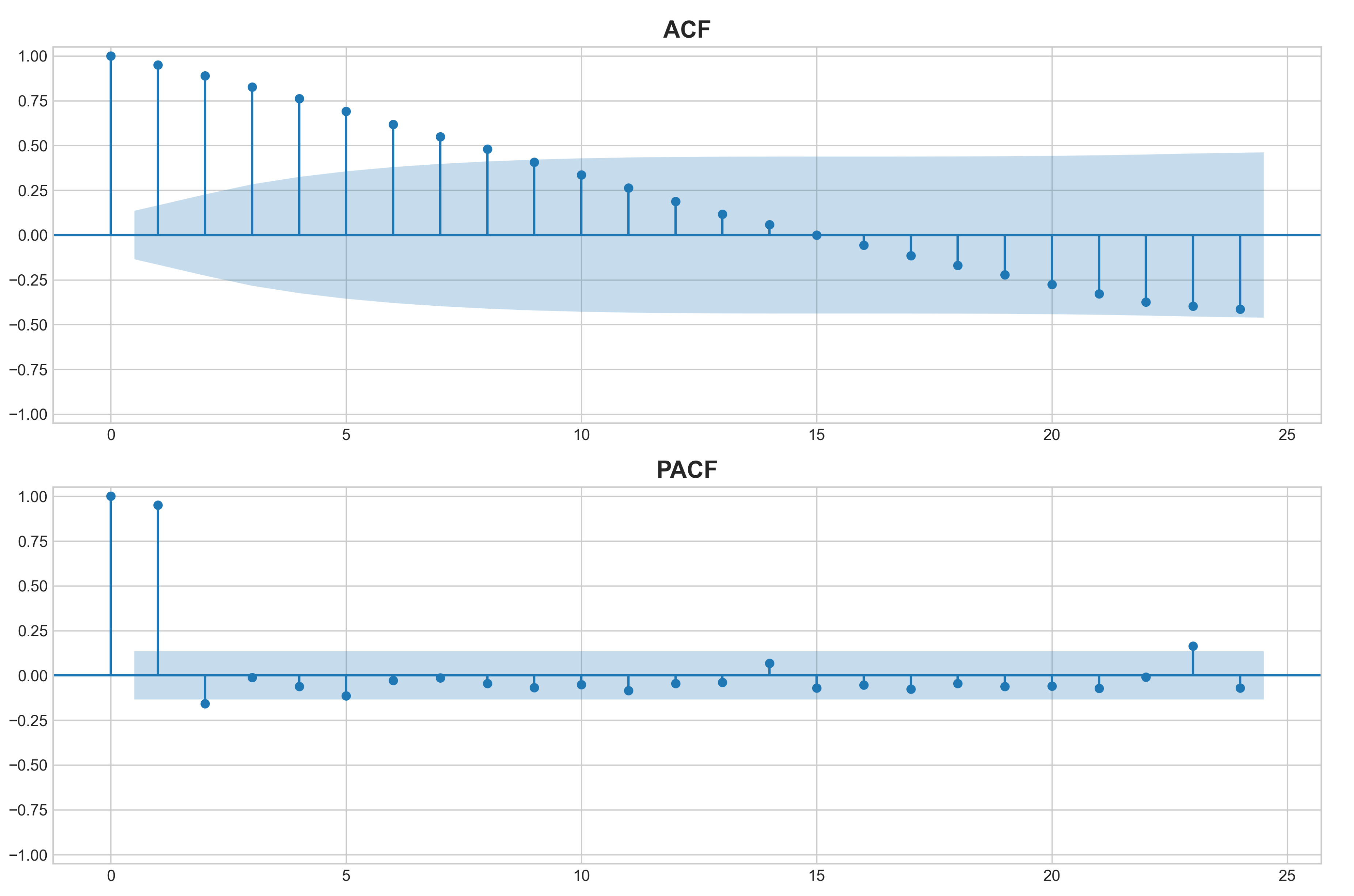
Figure 5.
Actual demand vs. predicted demand.
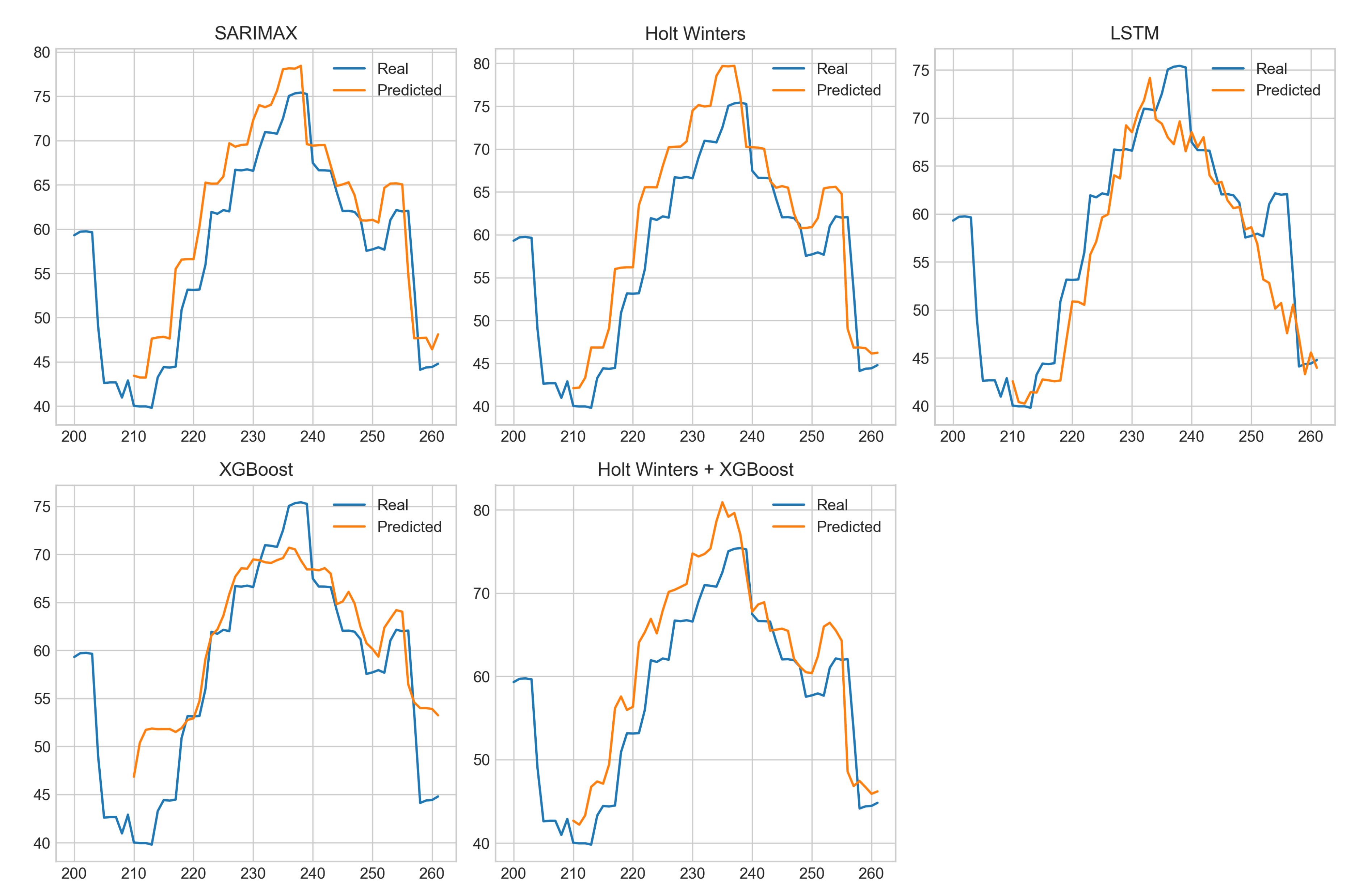

Table 1.
Experimental results of the evaluated models.
| Model | sMAPE (%) | TL (ms) | IL (ms) | Peak RAM (MiB) | Storage (kB) |
|---|---|---|---|---|---|
| SARIMAX | 1.21 ± 0.05 | 7740 ± 70 | 8.05 ± 0.09 | 408.23 | 116134 |
| Holt-Winters | 1.39 ± 0.06 | 183 ± 3 | 3.64 ± 0.08 | 236.58 | 31 |
| LSTM | 3.7 ± 0.1 | 19068 ± 1848 | 2100 ± 90 | 867.52 | 245 |
| XGBoost | 1.03 ± 0.04 | 54 ± 1 | 25.3 ± 0.1 | 359.58 | 112 |
| Holt-Winters + XGBoost | 1.36 ± 0.06 | 252 ± 2 | 29.9 ± 0.1 | 324.95 | 156 |
Disclaimer/Publisher’s Note: The statements, opinions and data contained in all publications are solely those of the individual author(s) and contributor(s) and not of MDPI and/or the editor(s). MDPI and/or the editor(s) disclaim responsibility for any injury to people or property resulting from any ideas, methods, instructions or products referred to in the content. |
© 2025 by the authors. Licensee MDPI, Basel, Switzerland. This article is an open access article distributed under the terms and conditions of the Creative Commons Attribution (CC BY) license (http://creativecommons.org/licenses/by/4.0/).
Copyright: This open access article is published under a Creative Commons CC BY 4.0 license, which permit the free download, distribution, and reuse, provided that the author and preprint are cited in any reuse.


