Submitted:
10 September 2025
Posted:
11 September 2025
You are already at the latest version
Abstract
Efficient simulation of tumor growth using cellular automata (CA) requires high computational power, especially when scaling to large biological systems. In this paper, we present a GPU-accelerated dynamic load balancing strategy for tumor growth simulation, using CUDA to optimize execution and scalability. We compare our approach with traditional CPU implementations and static load balancing methods, and demonstrate significant performance gains. Our results show that the proposed strategy reduces execution time by up to 54% for a 1024×1024 grid of CUDA thread blocks while maintaining accuracy, making it a promising approach for large-scale biomedical simulations.
Keywords:
cellular automata
; tumor growth model
; CUDA
; parallelization
1. Introduction
Tumor growth simulation is a very important field of biomedical research today, as it is an invaluable aid in better understanding cancer progression and can be crucial in the development of personalized cancer treatments. Thus, by modeling tumor growth dynamics using high-performance computing (HPC), researchers can predict the behavior of tumors under certain conditions, optimize medication delivery strategies, and evaluate the efficacy of treatments before conducting clinical trials [1]. The acceleration now provided by GPUs has significantly improved the accuracy and scalability of the aforementioned simulations, enabling large-scale, biologically realistic models that until recently were computationally infeasible [2]. Together with other machine learning techniques, tumor growth simulation is paving the way to precision oncology and better patient outcomes [3].
- Despite extraordinary advances in computational modeling, tumor growth simulations still face significant challenges in terms of improving efficiency and enabling non-hardware-limited scalability. Traditional mathematical models, based on cellular automata (CA) [4] and reaction-diffusion differential equations, require very high computational power, especially to implement realistic biological simulations. Scalability issues arise from the complex interactions between tumor cells, the microenvironment, and responses to cancer treatments, which require models with high spatial and temporal resolution [5]. In addition to all of the above, adapting the above models to modern heterogeneous architectures, such as GPU clusters or distributed HPC systems, remains a challenge for researchers due to inefficient load balancing between processors, memory bottlenecks, and constraints [6] to achieve maximum computational parallelization. Solving all these open problems is currently crucial to achieve real-time simulations that support clinical decision making and personalized treatment strategies.
-
Parallel computing has proven its effectiveness in many application domains related to the simulation of complex processes and is now enhanced by distributed HPC and heterogeneous architectures offered by GPUs. We can mention numerous works that have managed to improve the efficiency of CA implementations [7,8] in the field of tumor growth simulation. Even so, and due to the very process of the restrictions imposed by parallelization, the expected computational efficiency is significantly reduced. This usually occurs because the sharing of data or partial results leads to race conditions between processors, which have to be solved with synchronization between processors, limiting their parallelism potential [9,10]. [11] proposes a tumor growth model using a parallelized CA, which includes a dynamic balancing strategy of cells to be processed among multiple threads in execution and introduces adjustable parameters, depending on the different conditions that arise during the execution of the simulation. Other approaches currently seek to obtain computational dynamic load balancing, which can be found in [12], which presents dynamic load balancing techniques for the efficient parallel execution of a CA in a two-dimensional domain divided into rectangular regions. In [13] the load balancing was achieved on a two-dimensional processor grid as required by the geometry of the problem.The scalability of GPU-based tumor growth simulations is significantly enhanced by avoiding costly synchronization between GPU block threads and maximizing parallel execution efficiency. Unlike the [11] approach, which processes each tumor cell independently and requires synchronization for updates to shared data, we revisit and redefine the [4] model to ensure that each grid cell’s state is updated independently in the next iteration of the algorithm. This method guarantees that each thread processes its own cell without requiring mutual exclusion mechanisms or atomic operations, thus eliminating contention overhead. By structuring the workload efficiently across GPU cores, we fully utilize the computational power of GPU multiprocessors, achieving higher concurrency and better load balancing. This significantly improves execution time and scalability compared to traditional CA-based parallel models.
-
Contributions of this paper:
- –
- A novel dynamic load balancing strategy for GPU-accelerated CA-based tumor simulations.
- –
- A performance comparison against CPU and static GPU approaches.
- –
- Analysis of scalability and efficiency improvements.
2. Related Work
- The modeling of tumor growth has been carried out using cellular automata (CA) due to their capacity to capture very complex biological behavior by defining simple local rules [4]. CAs are discrete computational models whose representation consists of a grid of cells whose state evolves each following a set of rules that determines its state in the next simulation step. CA-based models can be used to simulate tumour growth, the invasion of tissue by tumor cells, and interactions with the surrounding microenvironment. Unlike continuous models, such as reaction-diffusion equations [14] and ordinary differential equations [15,16] with boundary conditions to capture the stochastic nature of interactions between cells, CA-based models offer a very powerful alternative as they explicitly simulate the individual behavior of cells and allow the evolution of tumors to be studied at different scales. The paper [17] provides a comprehensive review of computational models of the cell cycle in tumors, emphasizing the importance of understanding the proliferation of cancer cells. This review discusses various modeling approaches, including CA models, and their application to the simulation of cell life cycle dynamics and their response to different therapeutic interventions. As computational power increases and more biological data becomes available, CA-based models will become the cornerstone of personalized therapies and the development of new cancer treatment strategies.
- Parallelization techniques are fundamental to implement efficient AC model-based simulations. Recently, significant progress has been made in optimizing AC simulations using different computational strategies. For example, in [18] a scalable solver for a personalized breast cancer therapy is developed using a hybrid stochastic CA model. In [19] techniques such as frameworks for stencil computing are explored to optimise CA simulations on GPUs, resulting in significant performance improvements. Similarly, [20] explores parallel CA implementations, demonstrating that leveraging GPUs and multicore CPUs can significantly speed up simulations. All these studies underline the importance of using parallelization methods to improve the efficiency and scalability of CA-based simulations.
- Load balancing plays a critical role in High Performance Computing (HPC) for CA-based simulations, ensuring that computational resources are optimally utilized. Dynamic load balancing (DLB) methods, such as domain decomposition and workload redistribution, are often used to evenly distribute tasks across processors. However, these approaches face inherent limitations, especially in spatially heterogeneous CA-based models where the computational load varies dynamically. [11] propose a parallel CA tumor growth model that integrates dynamic load balancing, significantly reducing execution time compared to sequential implementations. However, their study highlights the synchronization overhead as a major drawback when balancing the load across multiple computational threads. Similarly, [12] develop a closed-form analytical solution for computing optimal workload assignments in distributed memory architectures using MPI-based dynamic load balancing. Their approach improves performance by reducing idle times between nodes, but struggles with communication bottlenecks caused by frequent workload redistribution. In both studies, the trade-off between load balancing frequency and overhead cost remains a key challenge. While dynamic partitioning techniques improve resource utilization, they also introduce significant computational overhead, especially in CA models where local interactions evolve unpredictably over time. Therefore, achieving an optimal balance between computational efficiency and synchronization costs in HPC-driven CA simulations remains an open research problem.
- CUDA and GPU acceleration play a critical role in improving the performance of CA-based tumor growth simulations, enabling large-scale and high-resolution modeling of tumor dynamics. [11] proposed a parallel CA tumor growth model with dynamic load balancing, which significantly reduced execution times compared to sequential implementations. Their work highlights the importance of efficient parallelization strategies to overcome computational bottlenecks in large-scale tumor simulations. Recent developments in GPU-based CA models continue to demonstrate significant improvements in simulation speed and scalability. [21] presented Gell, an open-source, GPU-based 3D hybrid simulator capable of handling tens of millions of cells, achieving a 150-fold speed-up over parallel CPU methods. Similarly, [19] optimized stencil-based CUDA implementations of CA, demonstrating significant performance gains for large-scale simulations. These studies highlight how CUDA-based parallelization and GPU acceleration are reshaping computational oncology by enabling more realistic tumor modeling while reducing computational costs. However, challenges remain in load balancing, memory constraints and inter-thread communication overhead, requiring further advances in hybrid parallelization strategies that leverage multi-GPU architectures and adaptive workload distribution.
3. Methodology
3.1. Tumor Growth Simulation Model
The Cellular Automata (CA) model focuses on the simulation of tumor growth through local rules that govern the behavior of each cell according to its immediate environment. The model can be described by the following triad: (Spatial Representation, Behavioral Rules and Model Assumptions).
-
Spatial representation:
- A discrete 2D grid is used in which each cell represents either a tumor cell or a surrounding tissue element (see Figure 1). The specific type of neighborhood used for interaction (e.g. Moore neighborhood with neighbors or von Neumann neighbourhood with neighbours) determines how each cell is affected by its environment.
- The system evolves in discrete time steps, which means that changes in the state of cells occur synchronously at regular intervals.
-
Behavioral rules. Each cell follows a set of probabilistic rules that influence three main parameters:
- Proliferation capacity ( ): Defines how often a cell can divide.
- Capacity for migration (): Determines the likelihood that a cell will move within the tissue.
- Spontaneous death capacity (): The probability that a cell will die without external intervention.
These parameters differ between cell types, particularly between tumor stem cells and tumor daughter cells. -
Model assumptions. The model assumes that tumor growth is driven by two types of cells:
- Tumor stem cells that are immortal (, ) and can generate both copies of themselves and tumor daughter cells.
- Tumor daughter cells that have limited proliferation () and a non-zero probability of death ()
Competition between cells for space is a key feature: If a cell has no available neighboring spaces, it enters a state of quiescence, i.e. it becomes inactive until conditions change.
This model provides a framework for studying tumour growth dynamics and can be optimized for high performance computing using parallelization techniques on GPU hardware.
3.2. GPU Parallelization Strategy
The CUDA-based implementation uses parallel processing on graphics processing units (GPUs) to accelerate tumor growth simulations. Key aspects of this implementation include addressing the following issues: (a) CUDA threading model and grid structure, (b) memory optimization, (c) synchronization and race condition handling.
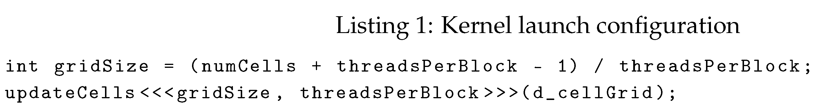
The computational domain is divided into a grid of thread blocks, where each thread is responsible for processing a single cell in the automaton:
- Each block processes a subregion of the grid, with threads assigned to individual cells.
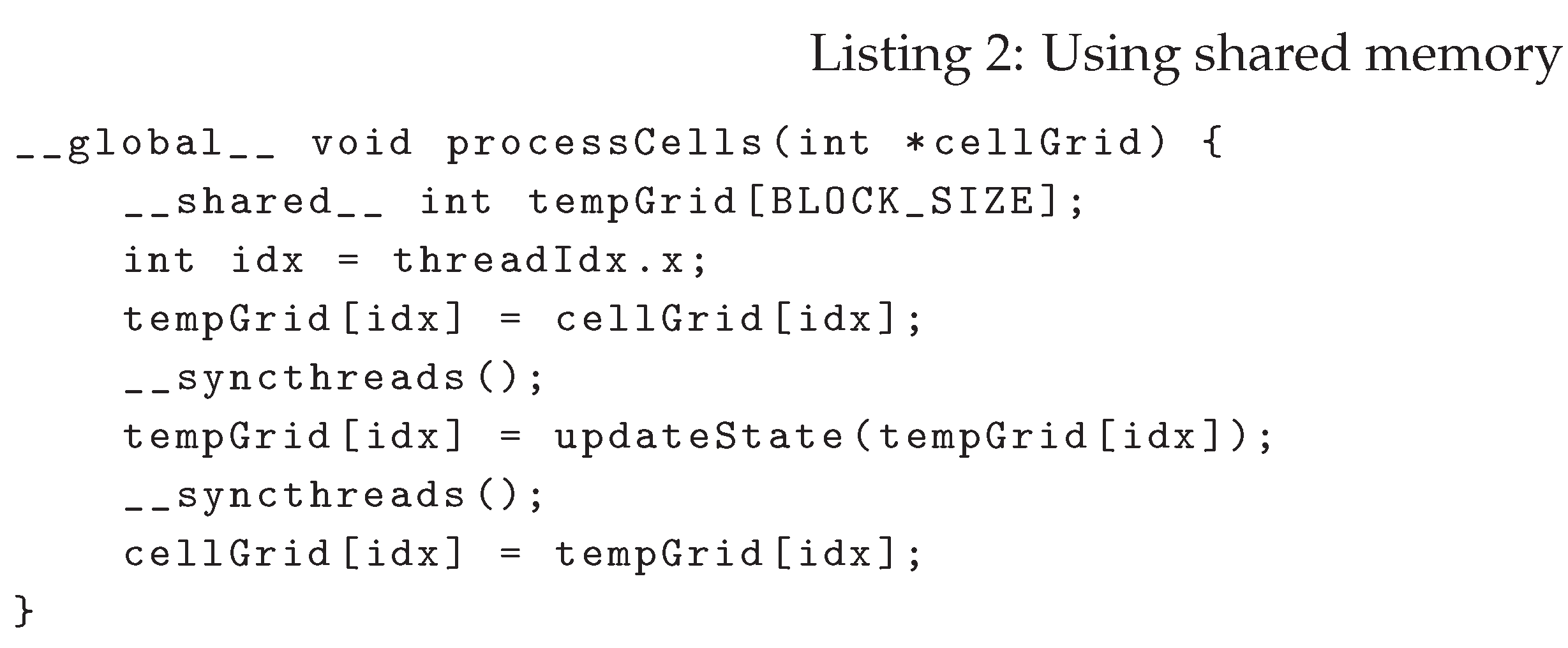
- Shared memory is used within blocks to store intermediate cell state updates, reducing global memory accesses.
- The number of threads per block is optimized for efficient memory access and computational load.
In terms of the memory optimization, the GPU-based implementation employs the following strategies:
- Shared memory: Used to store frequently accessed cell states within thread blocks.
- Global Memory Coalescing: Ensures that memory access patterns are optimized for Warp execution.
- Constant Memory: Stores static model parameters to reduce redundant memory fetches.
Proper synchronization mechanisms are used to maintain correctness and prevent the implementation from poor performance due to race conditions by using the specific constructs of CUDA:
- CUDA provides __syncthreads() to synchronize threads within a block, ensuring correct cell state updates.
- Atomic operations are used to prevent race conditions when multiple threads attempt to update shared memory locations.
- Grid-level synchronization strategies ensure consistent state updates across different blocks.
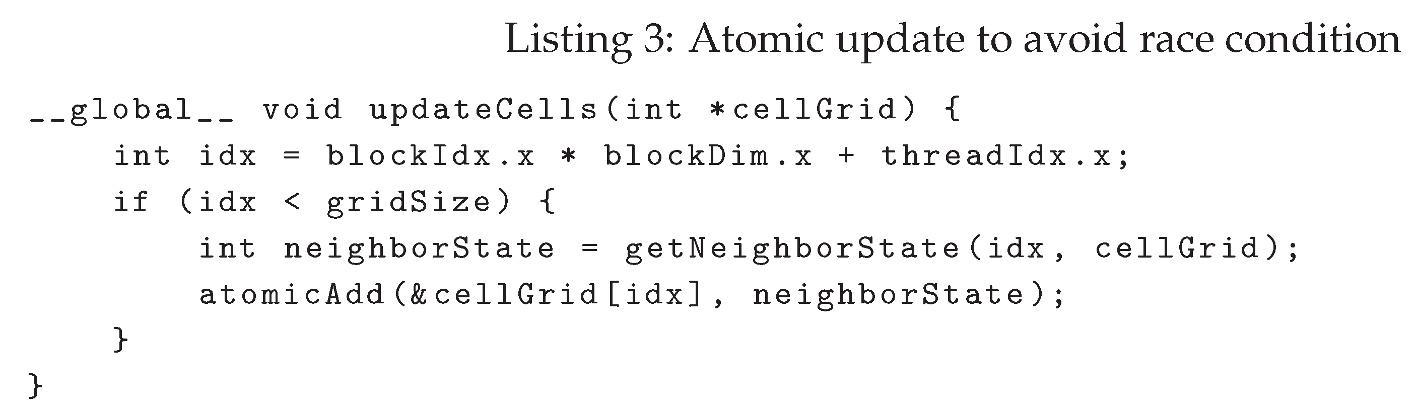
These approaches ensure that data remains consistent across threads while maximizing parallel efficiency. By using atomic operations and synchronization mechanisms, the implementation avoids race conditions and maintains the integrity of cell updates.
CUDA-based implementation of a CA can significantly improves computational efficiency, enabling large-scale tumor growth simulations to be performed in a feasible time frame.
4. Computational Model and Algorithmic Approach
The tumor growth simulation follows a structured computational approach based on cellular automata. The CUDA-based implementation leverages parallelization to efficiently model the stochastic evolution of tumor cells.
4.1. Computational Model
The CUDA implementation follows a parallelized probabilistic approach with the following key optimizations:
- Thread-based Parallel Execution: Each CUDA thread processes a single node in the 2D grid to ensure parallel execution of state updates.
- Double Buffering: Two grid states are maintained—one storing the current state, while the other holds the next iteration’s state—to prevent race conditions.
- Localized Computation: Cancerous transformation probabilities are dynamically computed using the Moore neighborhood.
- Memory Optimization: Random memory accesses are minimized by enforcing ordered neighbor processing.
Each neighbor is indexed systematically, starting from the upper left corner and proceeding clockwise (Figure 2). Neighboring cells containing cancer cells contribute to the probability of the cell transitioning to a cancerous state in the next iteration.
4.2. Demonstration of the -Cell Cancer Cell Generation Probability
This section presents the two cases for calculating the probability that the cell contains a cancer cell in the next iteration:
- -
- Case 1: does not initially contain a cancer cell.
- -
- Case 2: already contains a cancer cell and can either persist or receive a new cancer cell from its neighbors.
4.2.1. Definitions and Notation
Let be a cell in a grid that may or may not contain a cancer cell. We define the following terms:
- : the neighborhood of (typically a Moore neighborhood, consisting of up to 8 adjacent cells in 2D).
- v: the number of neighboring cells of that contain cancer cells.
- : the set of these cancerous neighboring cells.
- : the probability that a neighboring cell generates a cancer cell in , defined as:where is the number of nodes in that do not yet contain cancer cells.
- : the probability that a cancer cell in persists if it is already present.
- : the probability that a cancer cell migrates into from a neighboring cell.
4.2.2. Case 1: Probability of Cancer Cell Generation in
To compute the probability that at least one of the neighbors of will generates a cancer cell in , given that does not initially contain one, we consider all possible permutations of the set V. For a neighbor occupying position n in the ordering , the probability that it is the first to generate a cancer cell in is:
Probability of the first neighbour generating a cancer cell in .
Summing over all possible positions n where can generate the cell in , we obtain the total probability:
Final probability of cancerous transition in .
This equation expresses the probability that a cancer cell arises in due to the influence of its cancerous neighbors.
4.2.3. Case 2: Probability of Cancer Cell Persistence in
If already contains a cancer cell, the probability that it will persist in the next iteration or receive a new cancer cell is:
Probability of remaining cancerous or receiving a new cancer cell.
Here, represents the probability that the neighbor a generates a cancer cell in at position n:
Final probability contribution from all neighbouring cells.
Here, represents the probability of migration and reproduction from neighbour . All possible cases where is accessed after in the ordering are summed.
Finally, summing over all probabilities from each neighbor, we obtain the total probability formula:
Final probability of cancerous transition in .
This equation accounts for all possible contributions from neighbors, considering the order in which they are evaluated, ensuring the correct dynamics for persistence and generation of new cancer cells in .
4.3. Algorithm Description
The tumor growth simulation follows these key steps:
- Grid Initialization: Define the 2D grid with initial tumor cells and surrounding tissue.
-
State Update Rules:
- Proliferation: A tumor cell divides with probability if space is available.
- Migration: A tumor cell moves with probability .
- Apoptosis: A tumor cell undergoes programmed death with probability .
- Parallel Processing: Each cell is updated concurrently using CUDA kernels.
- Synchronization: Ensure proper data consistency across threads.
- Iteration Until Convergence: The simulation runs until steady-state tumor growth is achieved.
This optimized CUDA-based implementation significantly enhances computational efficiency and enables large-scale tumor growth simulations with high accuracy and performance.
4.4. Implemented CUDA Kernels
The simulation employs three specialized CUDA kernels for efficient parallel execution:
- Neighborhood Update Kernel: Scans the Moore neighborhood of each cell to compute the number of cancerous neighbors.
- Transition Function Kernel: Determines state transitions based on computed probabilities.
- Cancer Stem Cell Persistence Kernel: Ensures that cancer stem cells remain persistent throughout the simulation.
| Algorithm 1 Transition Function for Tumor Growth Simulation with CUDA |
|
The function calcProbabilities() in Algorithm 1 returns the probability of each neighboring tumor cell generating a cancer cell in , stored in a vector. The neighboring cell responsible for generating a cancer cell in is then accessed based on its probability. This sequence is further explained in Procedure 4, where the algorithms in Algorithm 2 or Algorithm 3 are invoked. These recursive algorithms compute the summation in Equation 4, adding one summand at each recursive call.
| Algorithm 2 Combinations of Probabilities if the Cell is Not Cancerous |
|
| Algorithm 3 Combinations of Probabilities if the Cell is Cancerous |
|
| Algorithm 4 Procedure for Probability Calculation in Cancerous Transition |
|
4.5. Algorithmic Complexity Analysis
The probability calculation procedure for cancerous transition involves nested loops, recursive function calls, and combinatorial operations that contribute to its overall computational complexity. Below, we analyze its complexity in detail.
4.5.1. Loop Complexity
The procedure consists of two primary loops:
- The first loop iterates over the variable from 0 to v, leading to a complexity of .
- The second loop iterates over the variable i from 0 to v, also contributing complexity.
4.5.2. Recursive Probability Computation
The probability calculations involve recursive functions, such as (Algorithm 2) and (Algorithm 3), which perform combinatorial operations. The worst-case scenario involves iterating over all subsets of v, leading to a complexity of:
Additionally, factorial terms appear in probability computations, suggesting that in the worst case, the complexity can reach:
4.5.3. Overall Complexity
Combining the loop and recursive components, the worst-case time complexity of the algorithm is:
However, in practical implementations, optimization techniques such as memorization or pruning redundant calculations can reduce the complexity to:
4.5.4. Parallel Execution Considerations
The CUDA-based implementation significantly improves performance by executing computations in parallel. Each CUDA thread processes a single grid cell, reducing the effective complexity per thread to:
Thus, leveraging GPU acceleration allows large-scale tumor growth simulations to be executed efficiently, even when handling complex probabilistic transitions.
4.6. Experimental Setup
The simulations were performed on an NVIDIA GeForce GTX 1650 with Max-Q design, using CUDA for parallel execution. The implementation used a dual-grid memory model to optimize GPU memory access and avoid race conditions by storing the state of the next iteration separately. The input dataset consisted of a structured 2D grid-based tumor growth model, with grid sizes of 512×512 and 1024×1024 nodes used for 25-day and 50-day simulations, respectively. A single stem cell was placed at the center of the grid as the initial condition, with each simulation step representing one hour, resulting in 600 steps for 25-day simulations and 1200 steps for 50-day simulations. The algorithm followed the Polesczuk-Enderling model [4], where tumor cell state transitions were governed by probabilistic rules based on neighborhood influence, including migration and reproduction probabilities. The performance evaluation focused on three key metrics: execution time, measuring the computational time required for each iteration; speedup, assessing the performance improvement of the GPU implementation over a sequential execution; and load balancing efficiency, analyzing the workload distribution across CUDA thread blocks. The execution strategy mapped each GPU thread block to a column of the grid, ensuring efficient parallel processing. The results showed a significant speedup over sequential approaches, although further optimizations in thread scheduling and workload balancing could improve performance even further.
5. Experimental Results
Since tumor growth simulations require a high resolution, we have chosen a grid to represent the tumor tissue. This grid size limits the tumor to 1,048,576 cells, which are initially empty (non-cancerous tissue) at the beginning of the simulation and can be progressively occupied by tumor cells. A grid of this size provides sufficient spatial resolution for meaningful biological modeling by ensuring that tumor progression, diffusion, and cellular behavior can be accurately simulated by the program. In addition, modern GPUs have multiple streaming multiprocessors (SMs) that can simultaneously process multiple blocks of 1024 threads, ensuring full utilization of all GPU cores across multiple SMs.
In our model, each thread processes a cell represented by a grid point. Since the grid is stored in a 2D array, the matrix can allow us to perform efficient memory access due to merged global memory read/write operations, row-major order access optimization since memory loads are sequential, and better cache locality since each warp processes a contiguous block of memory.
5.1. Performance Comparison
The performance of the proposed tumor growth simulation was evaluated using various execution parameters and CUDA grid configurations. The total execution time and the number of processed cells per time unit were measured with a grid over 150 simulation days. A comparison with previous work [11] highlights three key points: (a) the proposed algorithm processes a similar number of cells as in [11], demonstrating that the tumor growth model remains consistent. (b) Unlike [11], which used 4000 steps, this work uses 3600 steps to match the 150-day simulation time window, where each day consists of 24 steps, steps. (c) Although the best execution times of the proposed approach are slightly worse that those in [11], the grid cell distribution strategy enhances scalability, which was not achieved in the previous work.
5.1.1. CUDA Grid Size and Speedup Analysis
The speedup achieved when varying the CUDA grid size is detailed in Table 1. The results show a significant speedup compared to single-thread execution.
For small grid sizes, speedup is limited, but as the grid size increases, acceleration improves significantly. The best speedup () is observed at a CUDA grid, where the simulation achieves processed cells/s in only
5.1.2. Execution Time Curve Analysis
The relationship between number of tumor cells and execution time per step is crucial. Ideally, this relationship should be a linear or sub-linear, indicating that each thread runs independently. However, Figure 3a shows a slight curve, suggesting that cells interactions affect execution and the neighboring cells increase computational load.
Similarly, Figure 3b shows that total execution time initially increases rapidly as the tumor grows, but eventually, growth stabilizes and follows an approximately linear trend. This confirms that the probabilistic model remains efficient even for larger simulations.
5.1.3. Kernel Execution Analysis
Kernel execution times and GPU memory usage were analyzed using NvProf and Nsight compute tools. The results in Table 2 show that the most time-consuming processes are: (a) cell state updates and calculations (highest execution time); (b) memory transfers between GPU and CPU (every 5 simulation days); and (c) grid initialization and random number generation.
Regarding the occupancy analysis, Figure 4a shows that the initial kernel execution produces high occupancy, as most threads execute similar tasks. Over time, occupancy drops to 36.28% (Figure 4b), indicating imbalanced workload distribution. This suggests that GPU workload distribution to SMs could be further optimized to reduce occupancy drop and enhance overall efficiency.
5.2. Scalability Analysis
When designing a parallel implementation for GPU tumor growth simulations, the way the grid is partitioned will have a major impact on SM occupancy, memory access patterns, and load balancing. In this research, we explored two main approaches: (a) dividing the grid into 16 full rows or columns, (b) dividing the grid into 64 smaller regions to evaluate the performance of each region with respect to the GPU and to analyze the SM occupancy and cell processing distribution. A hybrid strategy (c) for optimized GPU utilization and memory efficiency is also discussed.
5.2.1. Dividing the grid into 16 rows and columns
The grid is split into 16 rows and columns, with each block processing an entire row or column. This makes it easy to allocate work to different GPU blocks. Memory is stored in a row-major order, so each thread processes a contiguous memory location, making memory accesses faster and more efficient. Threads in warp can also efficiently access contiguous memory locations, reducing memory latency.However, Figure 5 shows a severe SM under-utilization, as some Streaming Multiprocessors (SMs) exhibit minimal activity with only 6.3 million cycles, while others are significantly overloaded. The tumour grows from the centre of the grid outward, so the blocks responsible for the outer edges of the grid will finish their work faster than those processing the centre, causing some SMs to remain idle.The first few SMs process the centre, which is much denser (i.e. they will have a high workload), while other SMs process sparse areas (i.e. low workload), leading to underutilization of the GPU cores.
Figure 5 also shows that there is much lower L1/L2 cache utilization, resulting in a higher number of memory accesses being directed to DRAM rather than being efficiently cached. It also shows lower DRAM activity, but this is probably a result of SM under-utilization rather than an improvement in efficiency.
It is difficult to distribute work dynamically with this grid division strategy because the execution time of each block depends on the tumor density in the row or column assigned to it. This means that some blocks may be finished while others are still heavily processed.
5.2.2. Dividing the grid into 64 smaller regions
In this case, instead of assigning all of a row or column to one block, the grid is split into 64 smaller parts. Each block of threads then processes a part of a row or column spread across these different parts. As shown in Figure 6 using the CUDA Toolkit profiling figures, there is a lot more balanced SM utilization than in Figure 5 because all SMs take part within a narrow range of execution cycles (between 428 million and 443 million).
Dividing the grid into 64 regions is an effective way to improve GPU utilisation, as it makes sure that no SM is inactive. This approach makes it easier to balance the workload across the SMs, as shown in Figure 6. Since each block now processes small parts of cells spread across the grid, the workload is more evenly spread across the SMs. This strategy matches the tumor growth pattern (from the center of the grid to the edges) and is therefore less likely to create an imbalance because each SM receives work from multiple regions.In addition, since all SMs process similar amounts of work per iteration, there are fewer idle SMs, which keeps the GPU fully utilized.
Figure 6 shows that 64 regions is better at using L1/L2 caching, which reduces how long it takes to access global memory. This means that dividing the grid into 64 regions is more effective in keeping frequently accessed data in the cache, reducing DRAM bottlenecks and improving overall memory efficiency. It also means that more SMs are being used, and shows higher DRAM cycles, which indicates that more memory bandwidth is being used in computations. By dividing it into 64 regions, we make sure that the memory bandwidth is used efficiently. On the other hand, dividing it into 16 rows/columns leads to inefficient GPU execution due to idle or underloaded SMs.
This strategy also requires a more sophisticated indexing strategy to allocate blocks and ensure that work is distributed evenly across SMs. This results in more scheduling complexity in the SM schedulers.
5.2.3. Hybrid strategy
Instead of strictly dividing the grid into full rows or small regions, we combine both techniques to balance the memory access efficiency of the 16-row strategy with the load balancing of the 64-region strategy. This hybrid approach optimizes memory contention while ensuring high SM occupancy. The key components of the hybrid strategy are:
- Hierarchical grid partitioning. Each thread block is assigned a set of small contiguous row segments rather than full rows/columns or scattered regions, improving spatial locality.
- Coalesced memory accesses. Threads within a block process contiguous memory regions to enhance memory efficiency.
- Dynamic load balancing. Thread blocks dynamically adapt to workloads from different regions, preventing idle SMs and ensuring even resource utilization.
The hybrid approach ensures even workload distribution across all Streaming Multiprocessors (SMs). Unlike the 16-row division, where some SMs remain underutilized (as low as 6.3 million cycles), the hybrid method prevents imbalances by dynamically redistributing workload. It also outperforms the 64-region strategy by maintaining optimal SM active cycles, leading to near–uniform GPU utilization (Table 3).
Additionally, this approach maintains contiguous memory accesses, preventing excessive DRAM fetches and improving overall memory efficiency. By ensuring more localized memory access patterns, L1 and L2 caches achieve higher hit rates, reducing the need for costly global memory transactions. Compared to the 64-region strategy, which may cause scattered memory accesses and cache thrashing, the hybrid strategy ensures a more localized access pattern, leading to lower memory latency and improved overall performance.
5.3. Energy Efficiency & Resource Utilization
The use of memory for the cell grid division strategies in the GPU showed notable differences in the performance and the balance of the SM load. With the strategy of dividing the cell grid into 16 blocks, each block processes a complete row or column, which allows for the use of unified memory access, as this type of access is aligned with the way data is stored in the global memory of the GPU. Analysis by the CUDA Toolkit indicated that the shared memory usage per block was 48 KB, distributed efficiently among the concurrent threads. The size of the global memory space remained relatively low, as each block of threads operated sequentially on the row or column assigned to it in the distribution, resulting in minimal contention for access to the global memory.
The strategy of distributing the cell grid across 64 regions improved the load balance between the SMs, but increased latency due to access to global memory. This is mainly due to the fact that the thread blocks access the data following a more fragmented access pattern. In this case, the use of shared memory per block increased to 64 KB and, in addition, additional memory buffers were needed to manage the workload distribution. Meanwhile, the use of global memory increased by approximately 20% compared to the 16-block distribution strategy. Each block had to access more dispersed data, which increased cache error rates.
Analysis of the energy consumption of the strategy based on 16 rows and columns and the allocation of 64 regions of grid cells to the GPU’s SMs reveals notable differences in efficiency. Analysis of the CUDA Toolkit indicated that the SMs were not always busy with the first strategy, resulting in lower average energy consumption per execution cycle. Furthermore, this strategy benefits from reduced memory bandwidth usage, which is crucial for efficient GPU consumption.
On the other hand, the 64-region distribution strategy results in higher energy consumption, as it increases SM activity throughout the computation and because the blocks use more fragmented memory access patterns. The measurements show that all the SMs were active for many more cycles and that the lack of contiguous memory access caused higher energy costs per memory transaction, making this strategy less energy efficient compared to the 16-block strategy.
We can conclude that the strategy based on the distribution of 16 blocks was the most energy-efficient option, as it minimized the overhead due to data transfers in memory and optimized the number of execution cycles. The distribution strategy based on 64 blocks provided a much better computational load balance, although it increased energy consumption. Consequently, it seems that future optimizations could focus on hybrid memory allocation strategies to mitigate energy inefficiencies and maintain computational performance.
6. Discussion
The results show that the probabilistic algorithm with different load balancing strategies significantly improves the efficiency of tumor growth simulations using GPUs to achieve greater acceleration. The execution time scales sublinearly with the number of tumor cells in the mesh, so we can say that the implementation efficiently distributes the computational load among the SMs. The execution time per simulation step shows a slight non-linearity due to the interactions between tumor cells during the process, which could cause restrictions in memory access and overloads due to synchronization. The hybrid workload distribution strategy has demonstrated its potential to optimize load balancing and memory access patterns, resulting in a more uniform utilization of GPU resources.
The results obtained with the CUDA Toolkit performance analysis suggest that most of the execution time is spent on cell state transition calculations and neighbor updates, which highlights the importance of optimizing the cooperation between threads, reducing unnecessary accesses to global memory and using shared memory more efficiently.
6.0.1. Strengths and limitations of the proposed approach
The proposed approach has several strengths and limitations. The load balancing strategies between SMs guarantee an even distribution of the computing tasks between the SMs of a GPU and significantly reduce execution time compared to the application of fully static load balancing methods. Furthermore, high scalability can be verified, as large simulation domains (for example, grids) are successfully managed while maintaining overall performance, making it ideal for biomedical applications.
The optimization of memory access achieved through the use of shared memory and unified memory, which enhances the contiguity of accesses, helps to significantly mitigate bottlenecks and improves computational efficiency. In terms of limitations, the proposed approach may result in a drop in SM occupancy in the final stages of tumor growth, in which CUDA SMs are underutilized due to the spatial heterogeneity of tumor growth, resulting in uneven GPU usage. Losses in energy efficiency are also observed, as the second workload-sharing strategy increases in-memory operations and synchronization overhead, resulting in higher energy consumption compared to the other proposed strategies. Finally, the complexity of the probabilistic calculations of the cell state transition function, with a computational cost , poses challenges for extremely large-scale simulations, despite the optimizations made through parallelization on the GPU.
6.0.2. Potential for Generalization to Other Biomedical Simulations
The proposed algorithm and the methodology for load balancing between SMs of a GPU can be generalized to various applications in the fields of medical biology and computational biology. In the simulation of cancer therapies, the proposed tumor growth model can be adapted to incorporate interactions between drugs and immune system responses, allowing predictive simulations for personalized medicine. In the field of regenerative medicine and tissue engineering, similar cellular automata models can be applied to simulate wound healing, tissue regeneration, and stem cell differentiation. Furthermore, in the modeling of epidemics, the framework proposed by the probabilistic cellular automaton can be used to simulate the spread of diseases in heterogeneous populations, which helps to plan the response to a pandemic and to make decisions in the field of public health.
7. Conclusion & Future Work
This paper presents a probabilistic algorithm with dynamic load balancing for GPU-accelerated tumor growth simulations. The proposed method showed significant improvements in execution time, scalability and load balancing efficiency compared to static approaches. By optimizing CUDA memory access patterns and dynamically distributing computational tasks, the algorithm achieved significant speedups while maintaining simulation accuracy. The experimental results highlight the benefits of a hybrid workload distribution strategy that effectively balances GPU utilization and improves computational performance.
Future research could extend this work to multi-GPU or distributed HPC environments, enabling large-scale biomedical simulations across multiple computing nodes. Implementing adaptive load balancing techniques for heterogeneous architectures could further improve performance and scalability. In addition, exploring more efficient CUDA optimizations such as asynchronous memory transfers, kernel fusion and adaptive thread scheduling could reduce execution overhead and improve energy efficiency. These advances would make the proposed methodology even more applicable to complex biomedical simulations and real-time clinical decision support systems.
8. Online Resources
The C++/CUDA implementation of the tumor growth simulation code is available at:
References
- Anderson, A.; Chaplain, M. Continuous and Discrete Mathematical Models of Tumor-Induced Angiogenesis. Bull. Math. Biol. 1998, 60, 857–900. [Google Scholar] [CrossRef] [PubMed]
- Rice, J.R.; al. . Accelerating Multiscale Tumor Growth Simulations Using GPUs. IEEE Trans. Biomed. Eng. 2018, 65, 1525–1536. [Google Scholar]
- Begg, R.; al. . Machine Learning in Cancer Research: Applications and Challenges. Nat. Rev. Cancer 2020, 20, 660–674. [Google Scholar]
- Poleszczuk, J.; Enderling, H. A High-Performance Cellular Automaton Model of Tumor Growth with Dynamically Growing Domains, 2013, [arXiv:q-bio.QM/1309.6015].
- Kim, H.; al. . Computational Challenges in Tumor Growth Modeling and Simulation. IEEE Trans. Biomed. Eng 2021, 68, 1223–1235. [Google Scholar]
- P. Macklin. Key Challenges in Multiscale Modeling of Cancer. Ann. Biomed. Eng. 2019, 47, 2263–2281. [Google Scholar]
- Giordano, A.; Amelia, F.; Gigliotti, S.; Rongo, R.; Spataro, W. Load Balancing of the Parallel Execution of Two Dimensional Partitioned Cellular Automata. 2022 30th Euromicro International Conference on Parallel, Distributed and Network-based Processing (PDP) 2022, pp. 205–210.
- Cicirelli, F.; Forestiero, A.; Giordano, A.; Mastroianni, C. Parallelization of space-aware applications: Modeling and performance analysis. J. Netw. Comput. Appl. 2018, 122, 115–127. [Google Scholar] [CrossRef]
- Gerakakis, I.; Gavriilidis, P.; Dourvas, N.I.; Georgoudas, I.G.; Trunfio, G.A.; Sirakoulis, G.C. Accelerating fuzzy cellular automata for modeling crowd dynamics. J. Comput. Sci. 2019, 32, 125–140. [Google Scholar] [CrossRef]
- Grama, A.Y.; Gupta, A.; Kumar, V. Isoefficiency: measuring the scalability of parallel algorithms and architectures. IEEE Parallel Distributed Technol. Syst. Appl. 1993, 1, 12–21. [Google Scholar] [CrossRef]
- Salguero, A.G.; Capel, M.I.; Tomeu, A.J. Parallel Cellular Automaton Tumor Growth Model. In Proceedings of the Practical Applications of Computational Biology & Bioinformatics; 2018. [Google Scholar]
- Giordano, A.; Rango, A.D.; Rongo, R.; D’Ambrosio, D.; Spataro, W. Dynamic Load Balancing in Parallel Execution of Cellular Automata. IEEE Transactions on Parallel and Distributed Systems 2021, 32, 470–484. [Google Scholar] [CrossRef]
- Rango, A.D.; Giordano, A.; Mendicino, G.; Rongo, R.; Spataro, W. Tailoring load balancing of cellular automata parallel execution to the case of a two-dimensional partitioned domain. The Journal of Supercomputing 2023, 79, 9273–9287. [Google Scholar] [CrossRef]
- Gatenby, R.; Gawlinski, E. A Reaction-diffusion Model of Cancer Invasion. Cancer Research 1996, 56, 5745–5753. [Google Scholar] [PubMed]
- Padder, A.; Shah, T.R.; Afroz, A.; et al. . A mathematical model to study the role of dystrophin protein in tumor micro-environment. Sci. Reports 2024, 14, 1–15. [Google Scholar]
- Yin, A.; Moes, D.; van Hasselt, J.; et al. . A Review of Mathematical Models for Tumor Dynamics and Treatment Resistance Evolution of Solid Tumors. Pharmacometrics & systems Pharmacology 2019, 8, 720–737. [Google Scholar]
- Gérard, C.; Goldbeter, A. Computational Models of the Cell Cycle: Past, Present, and Future. Nature Computational Science 2023, 4, 1–12. [Google Scholar] [CrossRef]
- Lai, X.; Taskén, H.A.; Mo, T.; Funke, S.W.; Frigessi, A.; Rognes, M.E.; Köhn-Luque, A. A scalable solver for a stochastic, hybrid cellular automaton model of personalized breast cancer therapy. International Journal for Numerical Methods in Biomedical Engineering 2021, 38. [Google Scholar] [CrossRef] [PubMed]
- Cagigas-Muñiz, D.; del Rio, F.D.; Sevillano-Ramos, J.L.; Guisado-Lizar, J.L. Efficient simulation execution of cellular automata on GPU. Simulation Modelling Practice and Theory 2022, 118, 102519. [Google Scholar] [CrossRef]
- Marzolla, M. , Parallel Implementations of Cellular Automata for Traffic Models. In Developments in Language Theory; Springer International Publishing, 2018; p. 503–512.
- Du, J.; Zhou, Y.; Jin, L.; Sheng, K. Gell: A GPU-powered 3D hybrid simulator for large-scale multicellular system. PLoS ONE 2023, 18. [Google Scholar] [CrossRef] [PubMed]
Figure 1.
Two-dimensional grids, for the cases where and , the neighbors adjacent to the nodes in yellow are shown in gray.
Figure 1.
Two-dimensional grids, for the cases where and , the neighbors adjacent to the nodes in yellow are shown in gray.
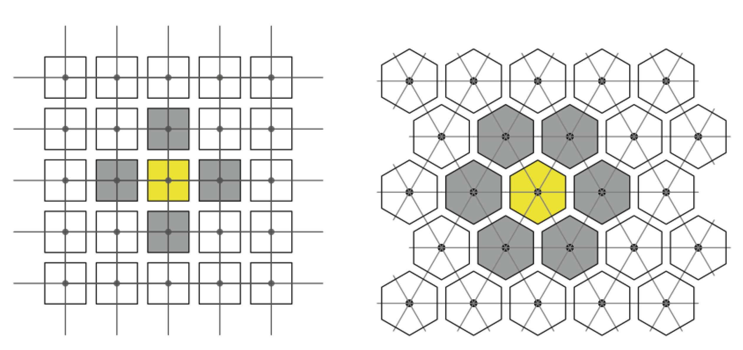
Figure 2.
Indexing of the neighbors of cell in the Moore neighborhood.
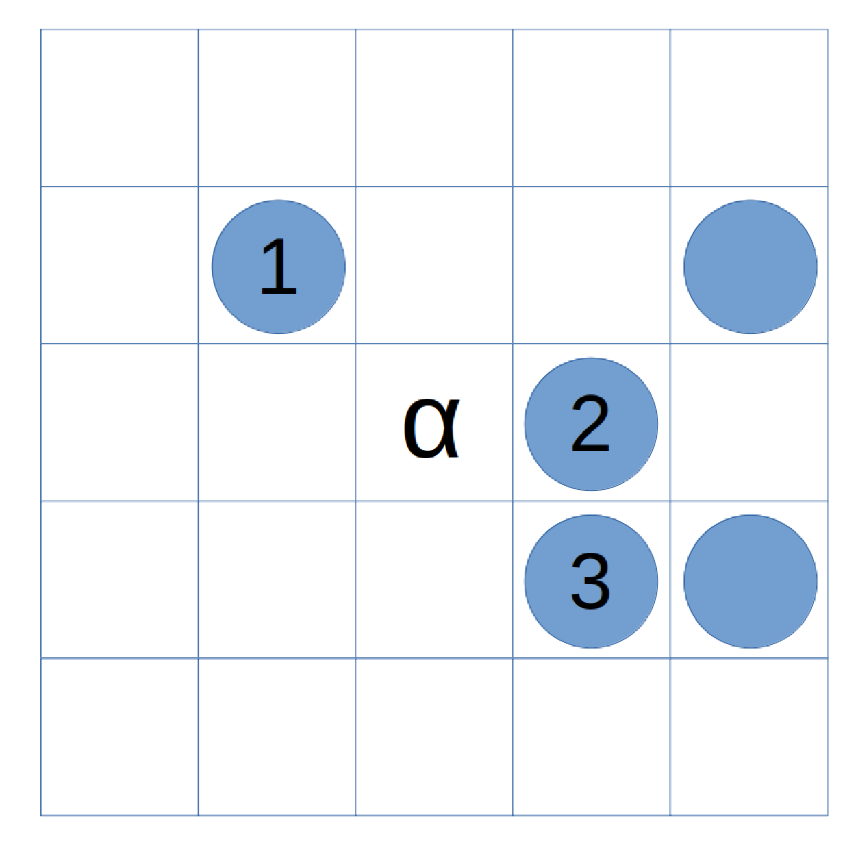
Figure 3.
Comparison between the number of cancer cells and simulation time. (a) Time per simulation step. (b) Total time for simulation.
Figure 3.
Comparison between the number of cancer cells and simulation time. (a) Time per simulation step. (b) Total time for simulation.
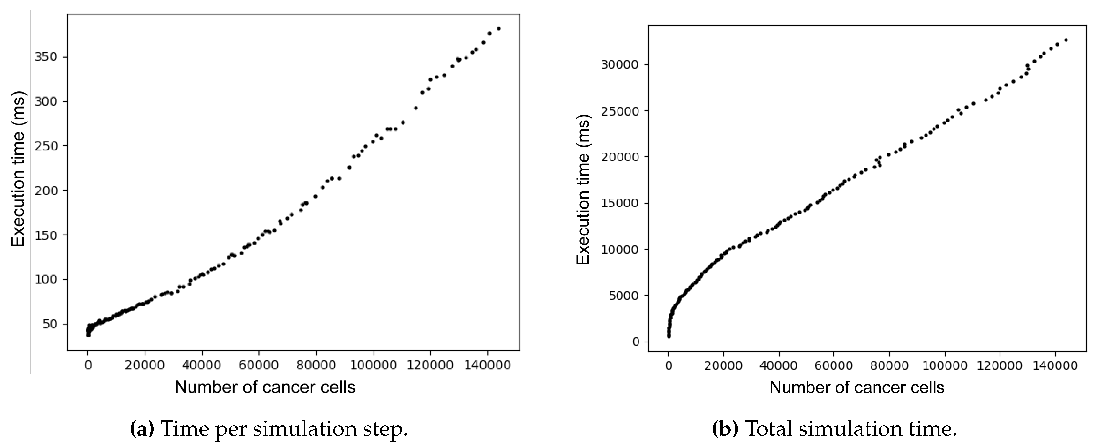
Figure 4.
Result of the analysis of the transition function execution in different iterations. (a) First iteration. (b) Last iteration.
Figure 4.
Result of the analysis of the transition function execution in different iterations. (a) First iteration. (b) Last iteration.
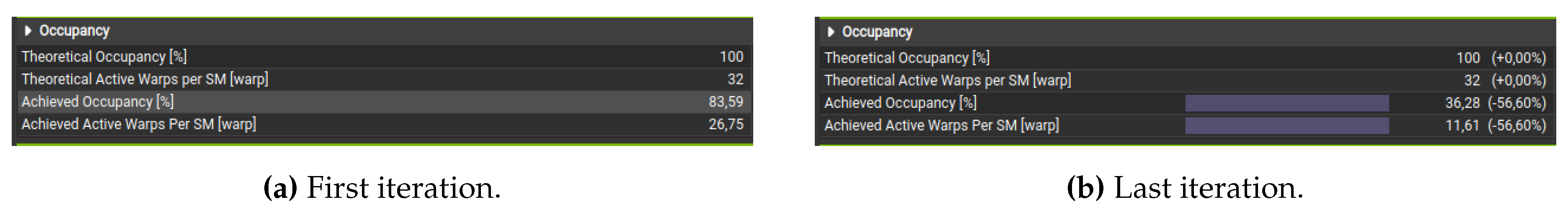
Figure 5.
Load distribution on the different SMs of the GPU for the distribution of the cell grid in 16 rows/columns.
Figure 5.
Load distribution on the different SMs of the GPU for the distribution of the cell grid in 16 rows/columns.
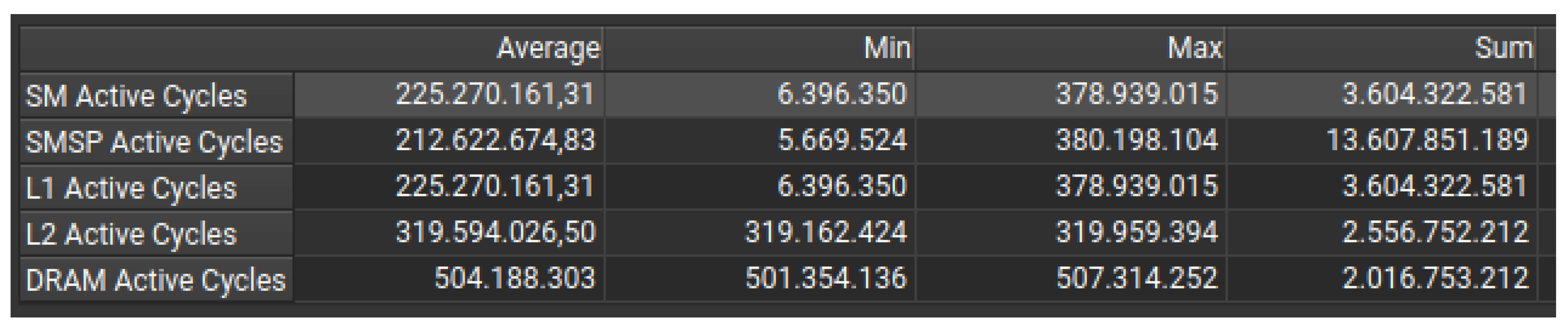
Figure 6.
Load distribution on the different SMs of the GPU for the distribution of the cell grid in 64 regions.
Figure 6.
Load distribution on the different SMs of the GPU for the distribution of the cell grid in 64 regions.
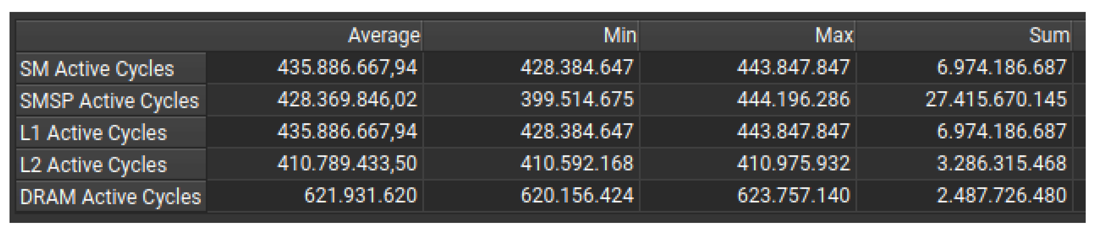

Table 1.
Performance of the simulations carried out with the probabilistic model, varying the size of the CUDA grid.
Table 1.
Performance of the simulations carried out with the probabilistic model, varying the size of the CUDA grid.
| CUDA Grid | Size | Processed | Processed/s | Seconds | Speedup |
|---|---|---|---|---|---|
| 1x64 | 164,401 | 191,918,090 | 40,234.41 | 4769.998 | 1 |
| 2x64 | 136,588 | 146,984,801 | 78,683.08 | 1868.061 | 1.956 |
| 4x64 | 153,697 | 173,264,862 | 84,914.98 | 2040.451 | 2.111 |
| 8x64 | 146,279 | 169,838,837 | 147,932.54 | 1148.083 | 3,677 |
| 16x64 | 146,784 | 160,235,895 | 250,391.66 | 639.941 | 6.223 |
| 16x16 | 147,533 | 176,305,011 | 136,524.60 | 1291.379 | 3.393 |
| 32x64 | 137,424 | 154,349,732 | 498,481.24 | 309.64 | 12.389 |
| 32x32 | 158,803 | 180,625,230 | 262,416.52 | 688.315 | 6.522 |
| 64x64 | 141,702 | 161,861,208 | 908,587.38 | 178.146 | 22.582 |
| 128x128 | 119,016 | 123,115,379 | 2,344,429.65 | 52.514 | 58.269 |
| 256x256 | 139,710 | 147,640,588 | 4,906,306.92 | 30.092 | 121.943 |
| 512x512 | 129,254 | 142,093,466 | 5,581,705.07 | 25.457 | 138.729 |
| 1024x1024 | 134,349 | 151,196,626 | 8,797,150.52 | 17.187 | 218.647 |
Table 2.
Kernel execution times and execution times examined using Nvprof.
| Kernel / Operation | Time (%) | Total Time | Calls | Avg Time | Min Time | Max Time |
|---|---|---|---|---|---|---|
| transitionFunction() | 80.76% | 169.448s | 3600 | 47.069ms | 5.3988ms | 175.90ms |
| updateNeighbors() | 18.41% | 38.6204s | 3600 | 10.728ms | 10.392ms | 11.412ms |
| CUDA memcpy DtoH | 0.77% | 1.61256s | 31 | 52.018ms | 51.493ms | 53.980ms |
| setup_kernel() | 0.03% | 65.804ms | 1 | 65.804ms | 65.804ms | 65.804ms |
| CUDA memcpy HtoD | 0.02% | 51.896ms | 1 | 51.896ms | 51.896ms | 51.896ms |
| stemCellTest(Cel) | 0.01% | 18.802ms | 3600 | 5.2220µs | 2.3040µs | 7.3920µs |
Table 3.
Comparison of Workload Distribution Strategies.
| Factor | Comparison of Workload Distribution Strategies | ||
|---|---|---|---|
| 16 Rows/Columns | 64 Regions | Hybrid Grid (Expected) | |
| SM Utilization | |||
| × Poor | √ Good | √ Best | |
| Some SMs barely active | Better, but some | No idle SMs, | |
| minor imbalances | optimal load balancing | ||
| L1/L2 Cache Usage | |||
| × Lower efficiency | √ Better caching | √ Optimal cache utilization | |
| but could be optimized | reducing DRAM dependence | ||
| DRAM Usage | |||
| × Lower, but inefficient | √ Higher but | √ Balanced memory throughput | |
| SM execution | some contention | and compute execution | |
Disclaimer/Publisher’s Note: The statements, opinions and data contained in all publications are solely those of the individual author(s) and contributor(s) and not of MDPI and/or the editor(s). MDPI and/or the editor(s) disclaim responsibility for any injury to people or property resulting from any ideas, methods, instructions or products referred to in the content. |
© 2025 by the authors. Licensee MDPI, Basel, Switzerland. This article is an open access article distributed under the terms and conditions of the Creative Commons Attribution (CC BY) license (http://creativecommons.org/licenses/by/4.0/).
Copyright: This open access article is published under a Creative Commons CC BY 4.0 license, which permit the free download, distribution, and reuse, provided that the author and preprint are cited in any reuse.


