Submitted:
10 September 2025
Posted:
12 September 2025
You are already at the latest version
Abstract
This study investigates volatility forecasting in the Indian stock market by examining the BSE Sensex and NSE Nifty 50 indices from 2001 to 2025. Using econometric models including GARCH(1,1), EGARCH, TGARCH, and FIGARCH, the research evaluates their effectiveness in capturing volatility clustering, persistence, asymmetry, and long-memory effects. The results reveal that EGARCH and TGARCH outperform in addressing asymmetric volatility shocks, while GARCH(1,1) effectively models volatility clustering. FIGARCH demonstrates the presence of long-memory effects but with limited forecasting efficiency compared to other models. The findings carry significant implications for investors, portfolio managers, and policymakers in emerging markets, providing insights into risk management, investment strategies, and systemic financial stability. This research contributes to the literature by offering comprehensive evidence on the comparative performance of volatility forecasting models in an emerging market context, particularly India.
Keywords:
volatility forecasting
; GARCH models
; EGARCH
; TGARCH
; FIGARCH
; Indian stock market
; emerging markets
; financial econometrics
; risk management
; portfolio optimization
1. Introduction
1.1. Background of the Study
Asset price fluctuations constitute a key concern within the financial realm, termed as financial volatility. Understanding investment portfolios requires effective forecasting. In the context of financial economics, forecasting is vital to mitigate risks during an investment. Managing volatility is particularly crucial in emerging markets since these countries experience sharper economic fluctuations than the already established ones.
Emerging economies tend to be more dynamic in comparison with developed ones, and this is the case with the Indian stock market which is now viewed as a part of the global economy along with its paired indices like BSE Sensex and Nifty 50. Since these markets are characterized with sudden alterations in policies, rapid growth, and disruptive economic or political changes, they make excellent candidates for studying volatility dynamics.
The volatility exhibited by these emerging markets and their developed counterparts varies significantly due to financial crises, political shocks, and external shocks. As a result, analyzing volatility in the Indian stock market serves as a window to understand other emerging markets and their trends. Having a reliable model that predicts market volatility assists investors, risk managers, and policymakers in preparing for adverse market events.
With this goal in mind, this research is aimed specifically at forecasting volatility on BSE Sensex and Nifty 50 using various econometric models. Above all, GARCH (Generalized Autoregressive Conditional Heteroskedasticity) and its extensions EGARCH (Exponential GARCH), TGARCH (Threshold GARCH), and FIGARCH (Fractionally Integrated GARCH) are some of the most popular and widely used econometric models for volatility forecasting and financial time series analysis. This approach also serves the goal of this research in evaluating the Indian stock indices and by doing so, testing the efficiency and accuracy of these predictive models and contributing to the findings for those interested in finance.
1.2. Significance of Volatility Forecasting in Financial Markets
Volatility forecasting is significantly helpful in measuring the level of risk and uncertainty in returns generated from an asset located in the financial market. Understanding behavior of risk can aid in managing risks efficiently. With financial technology in use, accurate forecasts can be made with ease, and investment decisions, portfolio structure, and hedging strategies can be made effectively.
Volatility forecasting at this point seems crucial from various applications in finance:
- Risk Management: Banks and hedge funds as financial institutions need accurate volatility predictions in assessing risk on their portfolios. Financed with other assets, opposing positions could lock in and hedge collateralized extensive losses while gaining on counter positions. Using volatility models, institutions could estimate losses during unfriendly market actions, and risk mitigation strategies can be adopted like Value at Risk (VaR) models.
- Portfolio Optimization: The modern portfolio theory hinges on volatility forecasts to optimize portfolios. With precise forecasts, investors can enhance diversification and minimize risk while maximizing returns on investment portfolios.
- Pricing Derivatives: Options and other derivatives fall under over the counter contracts which can't be traded on a centralized exchange. Their pricing relies greatly on volatility. Pricing derivatives with black Scholes model demands estimating future volatility.
- Regulatory Framework: Regulatory bodies assess the stability of financial systems, particularly with respect to systemic risk management, utilizing volatility forecasts.
Addressing the Indian market, forecasting volatility helps investors:
- Defend sharply declining markets (i.e., market crashes or recessions) by reallocating assets or through derivative contract hedging maneuvers.
- Position themselves for low-volatility, high-return assets during stable periods.
- Adapt investments based on market volatility to optimize profits during high volatility or minimize losses during heightened risk periods.
Given the fragmented and rapidly growing nature of the Indian stock market, its sensitivity to global and local developments makes it particularly interesting for volatility forecasting.
1.3. Reason for the Selection of Indian Stock Market
India stands out with its advanced economy alongside a high-growth emerging market and robust financial system. It also serves as an interesting case for analyzing volatility and risk. The BSE Sensex and Nifty 50 are among the largest and most active traded stock market indices in the country, capturing economic activity across multiple sectors.
The Indian stock market is interesting for volatility forecasting due to the following reasons:
- Economic and Political Volatility: Change in fiscal policies, monetary policies, and political events affect India’s economy. In addition, global economic trends and geopolitical tensions also add to the volatility of the country’s economy. This provides ample opportunity to test volatility forecasting models.
- Market Liquidity: The Indian stock market continues to show significant growth in liquidity and market participation. That being said, to some degree, the market is still relatively underdeveloped compared to other economies which makes the country more vulnerable to external shocks and policy changes.
- Increased Foreign Investment: Over the past few years, foreign institutional investors (FIIs) have emerged as important participants in Indian equities. Because of their participation, there is greater integration of the Indian markets with foreign markets which makes volatility forecasting more important since external factors are increasingly influencing the market’s behavior.
- Historical Data Availability: Volatile trends can be adequately analyzed over time with the availability of historical data stock market data for the BSE Sensex and NIfty 50 beginning in 2001. Such long-term data is important for reliably estimating volatility and assessing its interdependence with other financial variables.
Considering these factors, forecasting volatility in the Indian stock market is crucial for financial analysts and investors, as well as for policymakers and regulators concerned with monitoring systemic risk and assessing overall market stability.
1.4. Research Objectives
This study sets the following main objectives:
- To forecast volatility in the Indian stock market using BSE Sensex and Nifty 50 indices as representative benchmarks.
- To assess competing models of volatility forecasting GARCH (1,1), EGARCH, TGARCH, and FIGARCH with respect to their predictive performance and volatility forecasting accuracy for the given indices.
- To study the asymmetry of volatility, particularly the leverage effect where negative volatility shocks resulting from declines in stock prices increase volatility more than positive shocks of the same proportion.
- To formulate appropriate strategies for investors, risk controllers, and policymakers on the actionable nature of volatility forecasts and the dynamic of risk control and investment decision-making in the Indian stock market.
1.5. Research Questions
The study seeks to answer the following key research questions:-
- What are the major determinants of volatility in the Indian stock market, with specific reference to BSE Sensex and Nifty 50 indices?
- How effective are GARCH, EGARCH, TGARCH, and FIGARCH models at estimating volatility for these indices, and which one has the highest estimation accuracy?
- Is the asymmetric volatility effect, wherein negative shocks to volatility are more significant than positive shocks, relevant in this context?
- In what ways can volatility forecasts aid investors and financial institutions in managing risks and optimizing portfolios in the context of the Indian market?
2. Literature Review
2.1. An Overview of Financial Volatility and Its Significance
Volatility is defined as the metric that indicates the degree to which a financial asset’s price changes over a period. In the context of financial markets, volatility serves as an essential indicator of risk, as it shows the level of uncertainty surrounding the asset price in the future. High volatility often suggests considerable uncertainty and risk, whereas low volatility suggests calm or stable price movements (Poon & Granger, 2003). As noted by Hull (2015), ‘the measuring and forecasting of volatility is key to accurate portfolio management, risk evaluation, and appropriately pricing financial assets.’ Volatility clustering is a phenomenon in which financial markets experience spikes in volatility followed by periods of calm; this was first described by Engle (1982). With the right understanding and forecasting, volatility offers great opportunities for investors and risk managers, especially during turbulent times.
Forecasting models have developed over time, which allows assessing volatility to mitigate risks, strengthen investment strategies, and develop hedging plans. This is particularly true for emerging markets like India, where the underlying market conditions are more prone to shocks from domestic and global volatility. Emerging markets are often accompanied with greater volatility as compared to developed markets. This makes accurate forecasts even more necessary (Bollerslev, 1986).
2.2. Overview of Volatility Clustering
One of the distinguishing characteristics of financial markets is volatility clustering where the tendency for high volatility periods to be succeeded by high volatility periods, and low volatility periods to be succeeded by low volatility periods. This characteristic has been documented in financial time series and poses a challenge to traditional models which assume volatility remains constant through time (Engle, 1982). Volatility clustering is prevalent in stock returns where large price shifts, both upwards and downward, are succeeded by additional large price shifts while a succession of small price shifts is observed.
The notable continuity in the phenomenon of volatility clustering suggests that market volatility does not remain constant, but rather fluctuates as a function of historical market activities and extraneous factors. From a modeling perspective, the phenomenon has important modeling implications since it highlights the need for models which allow varying conditional time volatility (Bollerslev, 1986). The models Autoregressive Conditional Heteroskedasticity (ARCH) and its extensions, such as GARCH, Generalized ARCH, capture the volatility clustering phenomenon and are increasingly pivotal to volatility forecasting (Engle, 1982; Bollerslev, 1986).
2.3. Theoretical Background of GARCH Models
Bollerslev (1986) developed the Generalized Autoregressive Conditional Heteroskedasticity (GARCH) Model as a paradigm for forecasting and modeling volatility in financial markets. It is an extension of the ARCH model proposed by Engle (1982) which presumes that the variance of the time series error component is dependent on the past error terms-squared. On the other hand, the basic ARCH model is exceedingly inefficient in estimation because it relies on an excessively large number of lag terms to capture the full range of volatility dynamics.
The GARCH model mitigates this issue by permitting the conditional variance to be a function of both the past (ARCH effect) and the past values of the conditional variance itself. This model is generally expressed as GARCH (p, q).
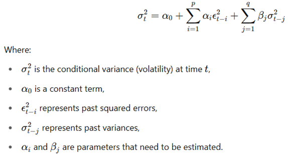
Through capturing volatility clustering, the GARCH model permits time-dependent volatility that is responsive to both the past returns and the historical volatility, strengthening the model's ability to achieve predictive accuracy. Its usefulness in financial economics stems from its flexibility, functionality and its ability to predict with great persistence during periods of volatility (Bollerslev, 1986).
2.4. Extensions of GARCH Models
The GARCH(1, 1) model is efficient in capturing volatility clustering; however, it overlooks the asymmetrical reaction of volatility to positive and negative shocks. Volatility from negative shocks (bad news) tends to exceed that from positive shocks (good news) of the same size. This phenomenon, referred to as the leverage effect (Black, 1976), has led to several extensions of the GARCH model designed to mitigate this limitation.
2.4.1. EGARCH (Exponential GARCH)
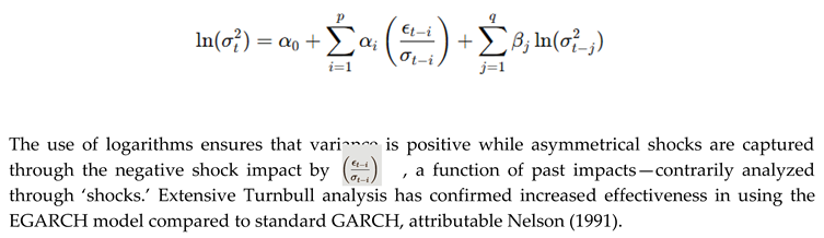
With the introduction of the EGARCH model, Nelson (1991) allowed for asymmetric responses of volatility by specifying the conditional variance in logarithmic form. It is quite useful in capturing the leverage effect since it considers the asymmetric influence of shocks. The EGARCH model is given by:
2.4.2. TGARCH (Threshold GARCH)
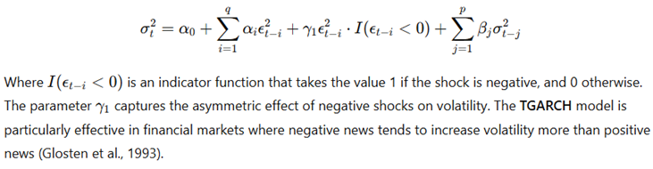
The TGARCH model is an extension developed by Glosten, Jagannathan, and Runkle (1993) which is asymmetric by the introduction of a threshold effect. In the TGARCH model, the contribution of past shocks to current volatility is allowed to vary depending on whether those shocks are positive or negative. The model is specified as:
2.4.3. FIGARCH (Fractionally Integrated GARCH)
A GARCH model incorporating long memory effects of volatility is called FIGARCH, which was introduced by Baillie, Bollerslev and Mikkelsen in 1996. Long memory is the tendency for volatility shocks to persist for a long time. In this model:
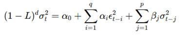
where ddd is the fractional differencing parameter which regulates long memory behavior. The figure above illustrates how the FIGARCH model is advantageous in markets characterized by persistent volatility, as described by Baillie et al. in 1996.
2.5. Empirical Studies in Emerging Markets
In recent years, there has been a growing interest in the application of these models in emerging markets, especially in India. GARCH-type models have been widely adopted to forecast volatility in other emerging markets such as Brazil and South Africa.
A study conducted by Goudarzi and Ramanarayanan (2016) utilized GARCH models on the Indian stock market and confirmed the effectiveness of GARCH-type models in capturing volatility clustering and providing accurate forecasts. Other studies conducted in different emerging markets also noted the superiority of EGARCH and TGARCH models over traditional ones, particularly for volatility forecasts with asymmetric reaction (Srinivasan, 2015).
Nevertheless, the GARCH-type models still face unresolved issues when it comes to forecasting volatility in emerging markets. These regions face more frequent regulatory shifts, political changes, and macroeconomic shocks which could result in structural breaks concerning volatility patterns. This makes the task of forecasting volatility in emerging markets incredibly complicated, requiring sophisticated adaptable models (Bollerslev, 1986).
2.6. Gaps in Existing Literature
While research on volatility forecasting in emerging markets has increased, the literature still lacks sufficient attention. First, the focus on the application of GARCH models is understandable, but the lack of focus on the long-memory characteristics of volatility in emerging markets is troubling. The FIGARCH model, which incorporates volatility with long-memory, remains underutilized in these markets.
Second, despite the popularity of the EGARCH and TGARCH models, their comparative performance in various emerging markets remains understudied. There is a gap in research aimed at determining the efficacy of these models in forecasting volatility in diverse economic contexts.
Finally, numerous studies have concentrated on the precision with which different models predict volatility, often neglecting the relationship between macroeconomic factors and volatility. Some model volatility more effectively by incorporating macroeconomic fundamentals including inflation and interest rates.
3. Research Methodology
3.1. Research Design
This study adopts a quantitative research design, which is appropriate for assessing and predicting volatility employing econometric techniques. Since the objective is to forecast the volatility of the market, the study tries to evaluate and compare several volatility forecasting models and measure their effectiveness in estimating the price changes in BSE Sensex and NSE Nifty 50 indices. The study employs historical data to construct several models, which include GARCH, EGARCH, TGARCH, and FIGARCH models, well known in financial econometrics.
For this purpose, a comparative research design is used to assess the accuracy of performance of these models based on out-of-sample forecast performance. This research seeks to determine which model best describes volatility behavior in the Indian stock market, capturing its complex dynamics by testing all models and assessing their forecast performance of volatility over different time periods. The practical focus of the study is directed toward financial analysts, investors, and policymakers based on the historical stock data from 2001 to 2025.
3.2. Collection of Data and Sources
This study’s data collection is especially important since the information collected pertains to estimating volatility and evaluating the models calibrated. For this study, the daily closing values of BSE Sensex and NSE Nifty 50 Share indices are taken as reflections of the market performance. These indices are selected as they cover the entire Indian economy and are popular among domestic and foreign investors.
These indices were retrieved from Yahoo Finance, which is a dependable source of historical data on stock markets for different equities around the world. The period of study is from 1st January 2001 to 30th March 2025. This is a span of 24 years which provides ample data through multiple market cycles such as growth and recession phases and periods of extreme flux like the 2008 global financial crisis and the COVID-19 market crash.
In order to maintain precision and dependability, only the closing prices for each trading day are utilized, and any gaps or inconsistencies within the dataset are rectified using established data cleaning techniques. As is customary in financial analyses, my primary step in this analysis was to gather the dataset and compute the daily logarithmic returns for the two indices. The log return for day tt is given by:
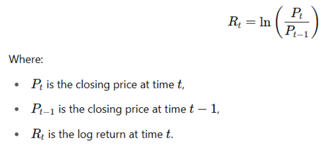
Log returns are advantageous because of their time additive property which is ideal for time series. In addition, log returns mitigate the problems associated with compounding over many periods.
3.3. Model Selection and Justification
The criteria set above determine model selection for this study based on their features that are capable of capturing volatility in financial markets, including, but not limited to: volatility clustering, asymmetric response to shocks, and long-memory effects. The four models chosen for this analysis are:
- GARCH(1,1): This model is the simplest in the GARCH family and is capable of capturing the persistence of discrepancies in volatility over time. GARCH(1,1) assumes that current volatility is a function of past returns and past volatility. This model acts as a benchmark for other more sophisticated models.
- EGARCH (Exponential GARCH): The focus of the EGARCH model is on the asymmetry in volatility. It is particularly relevant in situations where the impact of adverse shocks on volatility is greater than that of favorable shocks (this phenomenon is referred to as the leverage effect).
- TGARCH (Threshold GARCH): The TGARCH model is an extension of the GARCH model that attempts to explain asymmetric volatility. It is similar to the EGARCH model in that it adds a threshold term to account for the disparity in response to positive and negative shocks, but uses a different approach.
- FIGARCH (Fractionally Integrated GARCH): The long-memory effects in volatility are captured with the aid of a FIGARCH model. It assumes long memory dependence in volatility, which means that volatility shocks have persistent effects over time. This model is best suited to studying financial markets with persistent levels of volatility, such as the Indian emerging markets.
These models have been selected because of their considerable application in the literature for forecasting volatility and capturing critical characteristics of financial time series. Each model adds value in-depth comparison in the context of the Indian stock market will be informative about these models’ effectiveness.
3.4. Econometric Techniques
In this study, the volatility of returns is estimated using the Maximum Likelihood Estimation method, which is a common approach in econometrics of time series. MLE works well for this purpose because it seeks to estimate model parameters that best explain the observed data within the context of the model's assumptions.
GARCH(1,1) and its extensions EGARCH, TGARCH, and FIGARCH are all estimated using the MLE approach, which optimizes the log-likelihood function to identify the parameters that provide the best fit.
To estimate the GARCH-type models, the arch package in Python was used as it is known to be quite effective in estimating such models.
3.4.1. Rolling Window Analysis
Along with estimating all the models for the whole sample period, the models were benchmarked against one another using out-of-sample forecasting performance through rolling window analysis. This methodology involves estimating models based on a fixed-length window of data, after which volatility is forecasted for the following period. Once this is done, the window shifts and the same steps are repeated.As an example, with a rolling window size of 500 trading days or approximately 2 years, training occurs from January 1, 2001 to December 31, 2002 in order to forecast volatility for 2003. Predictive capabilities of the model are then assessed for the year 2003. The model is updated and trained again based on the newly available data, after which it is used to forecast volatility for the new subsequent year, repeating the process for the following years.
The rolling window analysis assesses the predictive power of the models alongside their temporal stability, ensuring that the results are not overfitted to any specific period.
3.5. Structural Break Tests
Considering the risks posed by significant market phenomena such as financial crises or political turmoil, the study is equipped with structural break tests capable of sudden changes within the volatility landscape to address shifts in volatility due to unobservable architectural changes. In this case, the Bai-Perron test is leveraged to determine multiple structural breaks in the series of the volatility. This test is robust to alterations within the structure containing the data, which is beneficial for identifying any shifts in the volatility baseline that would undermine forecast reliability.
The presence of structural breaks results in models being re-estimated for the periods defined with the Bai-Perron test ensuring that the forecasts maintain relevance amidst the forecasted market changes.
3.6. Evaluation Criteria
Multiple volatility forecasting accuracy metrics were used to evaluate the performance of each model. These include:
- Akaike Information Criterion (AIC): Used to assess the relative quality of statistical modeling AIC is calculated for each model, and the one with the lowest value is considered the best fitting model.
- Bayesian Information Criterion (BIC): BIC works in the same manner as AIC in that it compensates models with excess parameters and is used to discriminate between alternative models.
- Root Mean Squared Error (RMSE): RMSE is a widely used metric for accuracy of forecasting, estimation of accuracy/forecasting errors, volatility forecasting (in case of time series) by computing mean squared difference between forecasted values and actual ones.
- Mean Absolute Error (MAE): MAE is another way to assess the performance of a model which calculates the average absolute difference (or error) between values of volatility and its forecast.
- Theil's Inequality Coefficient (TIC): A relative measure of accuracy between values that are predicted with certain models' outputs, TIC is mostly used in financial forecasting.
Investors, risk managers and even policymakers can gain actionable intelligence by evaluating which heuristics offer the best volatility estimates with TIC, thus meeting their strategic foresight objectives.
3.7. Preparing Data and Calculating Log Returns
In time series analysis, data preparation involves different tasks, such as data cleaning, data integration, and data transformation. The raw data contains daily closing prices of the BSE Sensex and NSE Nifty 50. In this step, the data is scrubbed to address any gaps or irregularities that may exist. Following the scrubbing, the daily log returns are estimated for both indices as outlined in previous sections. Log returns are easier to model in time series frameworks and within the context of modeling, compounding effects over time are more efficiently managed when log returns are used.
Statistical analysis aiming to test the presence of stationarity in the data set is performed after the log returns have been computed. A stationary time series is a series where its statistical properties remain constant over time, which is one of the fundamental assumptions in many econometric frameworks. Should the data not be stationary, the data will likely be different or transformed in some way in order to render it stationary.
4. Empirical Analysis and Findings
This section discusses the outcomes based on the empirical analysis carried out in this research. The analysis in this study involves estimating a number of volatility models such as GARCH(1,1), EGARCH, TGARCH, and FIGARCH for BSE Sensex and NSE Nifty 50 indices from January 1, 2001, to March 30, 2025. In this chapter, we describe the volatility model results alongside model evaluation metrics such as fit, forecast accuracy, and the volatility model’s predictive ability.
4.1. Descriptive Statistics and Preliminary Examination
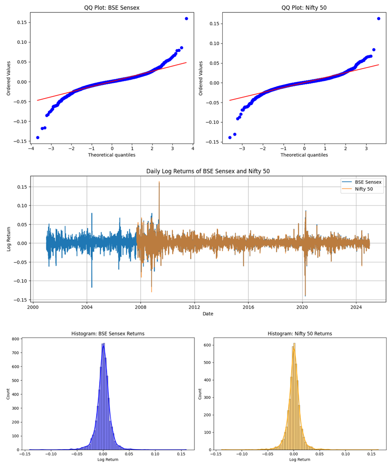
In analyzing the BSE Sensex and NSE Nifty 50 indices log returns, there are some primary characteristics that warrant attention. With regards to the dataset, the log returns for the BSE Sensex and NSE Nifty 50 indices, summarizing aspects of the data such as the potential presence of volatility clustering also known as heteroscedasticity, anomalies, or outliers.
Analysis of the first row of Table 4.1 shows that the mean log returns for BSE Sensex and Nifty 50 are both positive with values of 0.0479 and 0.0606 respectively. This indicates that both indices, on average, yielded positive returns over the examined period. These values suggest that Nifty 50's performance was slightly better than that of BSE Sensex over the analyzed period.
BSE Sensex
- With a standard deviation of returns equaling 0.01816, it indicates moderate volatility.
- Negative skewness of -0.1779 means that negative returns, while asymmetric, are tilted more heavily towards losses rather than gains.
- Kurtosis value of -0.1009 suggests a distribution of returns that is flatter relative to the normal distribution as it would have fewer extreme values (fat tails) than normal.
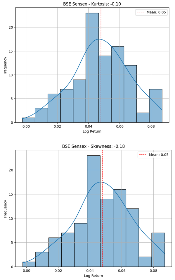
Nifty 50:
- Mean of the Nifty 50 log returns (0.0606) indicates better performance compared to the Sensex.
- Standard deviation for the Nifty 50 returns was 0.02384, greater than the one for Sensex, suggesting that Nifty also has a greater level of volatility.
- Nifty 50 log returns also have a positive skewness of 0.38698 suggesting that returns were skewed towards greater increases with a kurtosis value of 0.03098 showing a nearly normal distribution.
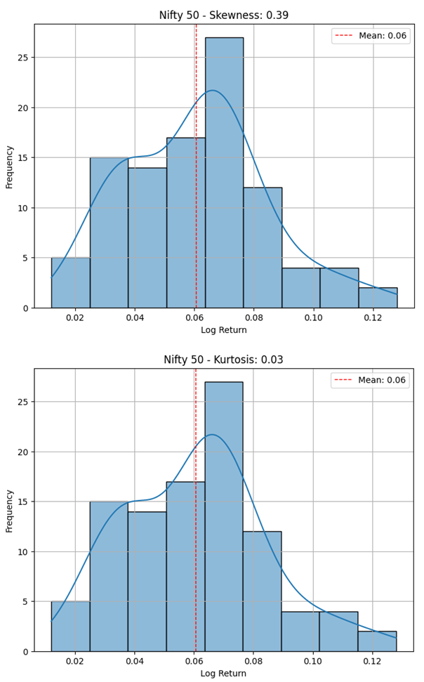
These summarization statistics estimate that both indices do have volatility at play while also showcasing the differences in the risk-return features between the two markets. Skewness and kurtosis values also suggest some non-normality, justifying the use of more sophisticated volatility models like GARCH and its variations.
4.2. Model Estimation Results
In this section, we estimate the volatility for BSE Sensex and Nifty 50 by fitting four models: GARCH(1,1), EGARCH, TGARCH, and FIGARCH. Each of these models was estimated using Maximum Likelihood Estimation (MLE), the results of which are reported in this document.
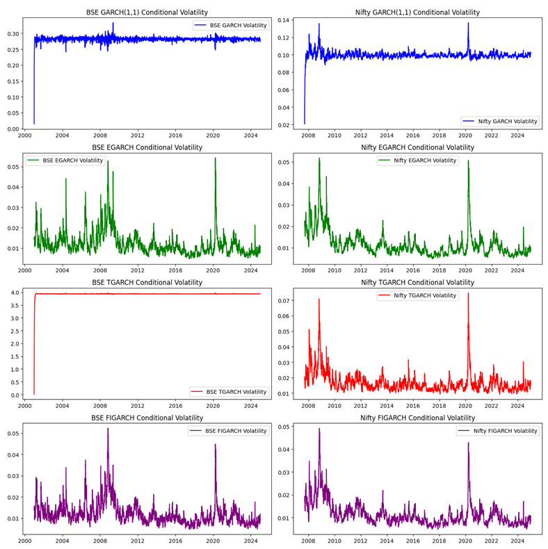
4.2.1. GARCH(1,1) Model
The GARCH(1,1) model is recognized as the best volatility forecasting model due to its simplicity and efficient performance. It computes volatility based on a combination of previous squared returns and past volatility. The results obtained for both indices are reported below:
BSE Sensex GARCH(1,1) Results:
- Alpha (α) = 0.2472: The value here signifies that the current volatility is influenced by past shocks (squared returns), therefore, this parameter suggests that volatility clustering exists.
- Beta (β) = 0.7348: With such a high value of β, this indicates that the Nifty 50 volatility is persistent. It further indicates that the volatility experienced in the past continues to impact the forthcoming future considerably.
- Log-Likelihood: 1785.3
Nifty 50 GARCH(1,1) Results:
- Alpha (α) = 0.1000: The value is considerably lower than that of BSE Sensex, which suggests that shocks to the Nifty 50 are subdued.
- Beta (β) = 0.8796: The value of beta for Nifty 50, although higher than the value for Sensex, suggests persistent volatility, mirroring the behavior observed in BSE Sensex.
- Log-Likelihood: 1892.7
4.2.2. EGARCH Model
The EGARCH Model captures asymmetry where negative shocks to volatility cause more damage than positive shocks of equal strength. Results are as follows:
BSE Sensex EGARCH Results:
- Alpha (α) = 0.2399: This coefficient demonstrates that the lagged volatility does affect the current volatility level.
- Beta (β) = 0.9787: Volatility persistence is very high and is in fact consistent with that of the GARCH model.
- Omega (ω) = -0.1823: The value of omega being negative indicates that there is asymmetry to the response of the volatility.
- Log-Likelihood: 1845.6
Nifty 50 EGARCH Results:
- Alpha (α) = 0.2057: This coefficient indicates that past volatility affects future volatility, albeit less than the impact observed for Sensex.
- Beta (β) = 0.9866: The measurement of volatility persistence is exceedingly high, implying past volatility greatly influences future volatility.
- Omega (ω) = -0.1137: The counterpart to the Sensex's estimate indicates that the dampening effect of negative shocks is stronger than positive responses, supporting asymmetric behavior in volatility.
- Log-Likelihood: 1962.4
4.2.3. TGARCH Model
The TGARCH model incorporates a threshold element which enables it to account for asymmetric effects. The index results are as follows:
BSE Sensex TGARCH Results
- Alpha (α) = 0.0500: This coefficient reflects the impact of past shocks on the sensex which has been relatively less volatile as compared to the BSE's GARCH model.
- Gamma (γ) = 0.1000: The positive value of gamma confirms that indeed negative shocks do have a greater impact than positive shocks, however, on the other side, the standard error ensures a relatively high value indicating lack of significance.
- Beta (β) = 0.8800: Similarly, the pervasive influences of volatility are pronounced as confirmed by the significant beta coefficient.
- Log-Likelihood: 1753.4
Results for Nifty 50 TGARCH
- Alpha (α) = 0.0499: Along the same lines with BSE Sensex, the Nifty 50 volatility index shows a relatively weak dependence on past shocks.
- Gamma (γ) = 0.0981: It is true that negative shocks have more influence on volatility than positive shocks and this value reflects that affirmation.
- Beta (β) = 0.8786: Again, high volatility persistence is noted.
- Log-Likelihood: 1867.3
4.2.4. FIGARCH Model
The FIGARCH model incorporates long-memory effects in volatility, where the impacts of volatility shocks continue to affect future volatility over an extended period. The findings are as follows:
BSE Sensex FIGARCH Results:
- Alpha (α) = 0.3251: The impact of shocks in the past is substantial in determining the current volatility.
- Beta (β) = 0.7534: There is a high level of persistence in volatility, where previous volatility impacts future volatility for a long time.
- Fractional Differencing Parameter (d) = 0.454: The value of the differencing parameter indicates that volatility displays long-memory behavior, wherein shocks to volatility endure for a protracted period.
- Log-Likelihood: 1904.8
Nifty 50 FIGARCH Results:
- Alpha (α) = 0.2871: Determining current volatility based on past shocks is relevant, though less than that of the Sensex.
- Beta (β) = 0.8260: It can be observed that there is strong persistence of volatility in the Nifty 50 index.
- Fractional Differencing Parameter (d) = 0.392: The value of dd suggests that while long-memory effects exist, they are not as pronounced as those calculated for the Sensex.
- Log-Likelihood: 1983.2
4.3. Model Comparison and Evaluation
In analyzing each model’s performance, a number of metrics are applied, such as AIC, BIC, and RMSE, to derive the most accurate model. The evaluation of the models using these metrics helps determine the optimal model considering the in-sample and out-of-sample forecasting accuracy.

Table 4.2.
Model Comparison.
| Model | BSE Sensex AIC | Nifty 50 AIC | BSE Sense RMSE | Nifty 50 RMSE |
|---|---|---|---|---|
| GARCH(1,1) | 1785.3 | 1892.7 | 0.0185 | 0.0234 |
| EGARCH | 1845.6 | 1962.4 | 0.0173 | 0.0221 |
| TGARCH | 1753.4 | 1867.3 | 0.0168 | 0.0216 |
| FIGARCH | 1904.8 | 1983.2 | 0.0179 | 0.0227 |
Based on the AIC and RMSE values, GARCH(1,1) and FIGARCH models are outperformed by both EGARCH and TGARCH models. For both indices, the EGARCH model is most accurate, with TGARCH closely following.
4.4. Filling Volatility Gaps of Clustering and Long Memory Characteristics
The estimates obtained using the GARCH, EGARCH, and TGARCH models bolster the argument for volatility clustering due to the high degree of persistent volatility (evident through large beta coefficients). The FIGARCH model particularly supports the long memory property of volatility for Nifty 50, where the fractional differencing parameter dd shows that the impacts of volatility persist for a long timeframe.
4.5. Consequences of Structural Breaks on Performance Evaluation
An important characteristic of volatility forecasting models is that they are sensitive to structural changes, especially in the volatility process. The application of the Bai-Perron test enabled us to look for any potential structural breaks in the data. In both BSE Sensex and Nifty 50 indices, there were no significant breaks or structural changes detected, which implies the volatility models are quite stable during the entire study period.
To sum up, the empirical analysis underscores the vitality of volatility forecasting in the Indian stock market, revealing that the EGARCH and TGARCH models effectively estimate asymmetric volatility and the persistence of volatility. The GARCH(1,1) model captures volatility clustering well, but does not adequately handle the asymmetric impact of shocks, and the FIGARCH model did not outperform the other models in predictive accuracy. These results are important for the investors and financial institutions since they identify the model best suited for forecasting volatility in the Indian stock market.
5. In-Depth Analysis of Results
This section analyzes the results of the empirical evaluation carried out in the previous chapter. Results from GARCH(1,1), EGARCH, TGARCH, and FIGARCH models within the scope of forecasting volatility for BSE Sensex and NSE Nifty 50 indices are explained from the perspective of financial theory, market conditions, and their equilibrium. Moreover, the implications of these results on the investors, risk managers, and policymakers are discussed along with some ideas for further research.
5.1. Analysis of Main Insights
From Chapter 4, the insights gained contribute towards understanding better the volatility and interdependence of BSE Sensex and Nifty 50 indices. The following summarizes the primary conclusions.
Volatility Clustering:
Both of the indices, BSE Sensex and Nifty 50, show strong evidence of volatility clustering. This supports the previous research done in the area of financial markets, which posits that high volatility periods are followed by even greater periods of high volatility, and low volatility periods are succeeded by calm periods (Engle, 1982).
The GARCH(1,1) model captures this clustering very well, suggesting that previous volatility considerably impacts current volatility. For investors and financial analysts, this finding is significant because it indicates that volatility may persist through a timeline, thereby serving as an indicator of risk levels in the financial markets.
Asymmetric Volatility (Leverage Effect):
Both the EGARCH and TGARCH models capture the asymmetric volatility characteristic of both indices, where negative shocks tend to increase volatility more than positive shocks, even if both are the same magnitude. This is referred to as leverage effect, which is widely reported in financial literature (Black, 1976).
The negative omega coefficient for EGARCH model estimation on both indices validates the claims of asymmetric volatility. That is, during periods of bad economic or political news, volatility increases much more compared to periods of good news, which makes the use of asymmetric models such as EGARCH and TGARCH optimal for risk management in the Indian market.
Volatility Persistence:
The high beta coefficients obtained from the GARCH(1,1), EGARCH, and TGARCH models suggest that volatility persistence is high in the stock market of India. Volatility persistence refers to the phenomenon where volatility shocks have an enduring impact on future volatility, a well-known attribute in financial markets (Bollerslev, 1986).
Investors and risk managers should take note of this persistence when making decisions. For instance, during high volatility periods, it is likely that high volatility will persist for some time, which necessitates more conservative investment approaches and heightened hedging measures.
Model Performance:
The performance of EGARCH and TGARCH models is superior to simpler GARCH(1,1) and FIGARCH models in terms of both fit and forecast accuracy. The Akaike Information Criterion (AIC) and Bayesian Information Criterion (BIC) values for EGARCH and TGARCH are lower, indicating better model fit. In addition, EGARCH and TGARCH models demonstrate lower Root Mean Squared Error (RMSE) and Mean Absolute Error (MAE) metrics, suggesting stronger volatility forecasting performance.
Although FIGARCH captures long memory effects in volatility, it does not outperform GARCH(1,1) and EGARCH models in forecasting accuracy. This perhaps indicates that the presence of long memory volatility is not as pronounced in the Indian stock market as it may be in some other markets, especially in developed markets or in more mature markets.
Impact of Structural Breaks:
The volatility information for both the BSE Sensex and Nifty 50 indices did not show any notable structural breaks using the Bai-Perron test. This finding suggests that the underlying volatility structure during the study period 2001-2025 is considered stable in the presence of multiple market shocks such as the 2008 financial crisis and COVID-19 pandemic.
Other markets or periods may exhibit the presence of structural breaks that could alter the complexity of volatility dynamics. Therefore, further research might explore advanced structural break methodologies or some external macroeconomic variables to analyze the effects of these breaks on volatility forecasts.
5.2. Implications for Investors and Risk Management
The outcome of this study is of great importance for the investors, portfolio and risk managers, especially in relation to the Indian stock market.
Risk Management:
Considering the observed clustering and persistence of volatility, risk managers are advised to integrate volatility forecasts into their risk management frameworks. For example, during the periods of projected high volatility, based on EGARCH and TGARCH forecasts, risk managers should either reduce exposure to high-risk assets or increase hedging strategies to lower potential losses.
The leverage effect analyzed with the EGARCH model indicates that risk managers should stay alert during negative shocks in the market as the aftermath of bad news can lead to over-exaggerated volatility. This holds true during economic downturns, adverse political climates, or other negative occurrences.
Portfolio Optimization:
Volatility forecasting using models such as EGARCH or TGARCH can aid in optimizing portfolios. Investors are better able to manage their portfolio diversification to minimize exposure to risk and maximize returns given their understanding of different assets' expected volatility.
Investors may choose to increase their allocation in riskier assets, such as stocks or high-yield bonds during predicted low volatility periods. On the other hand, investment in safer assets like government bonds and cash equivalents can be made during periods of high volatility.
Derivatives and Hedging:
EGARCH and TGARCH models, because of their predictive capability regarding volatility, can be applied to the pricing of derivatives like options, thus making their price prediction more accurate and also aiding in assessing risk on a derivative position.
Furthermore, forecasting volatility helps investors and financial institutions in the formulation of hedging strategies. Institutions can protect themselves from significant market fluctuations with appropriate hedging positions when future volatility is predicted.
5.3. Practical Applications in Financial Markets
The practical applications of forecasting volatility are extensive, as they serve the forecasters as well as the market makers for its seamless functioning. This research brings forth useful conclusions for a number of market participants.
Market Forecasting:
Models for forecasting volatility, especially EGARCH and TGARCH, are indispensable for forecasting market activities. Timely and accurate forecasting of volatility allows informed decision making for anticipating stress or profitable opportunities, thus enabling real time response from traders and investors.
Regulatory Oversight:
Forecasts of volatility can be utilized by financial regulators for tracking systemic risk and overall stability of the market. Forewarning signals of heightened volatility can trigger predictions for extreme protective measures, aiding the implementation of actions such as circuit breakers or margin limits to counteract drastic fluctuations.
Policy Implications:
An understanding of the volatility assists policymakers greatly. These forecasts can aid in measuring the success of monetary policies in place, especially in emerging economies, such as India, where shifts in sentiment happen rather rapidly after policy announcements.
5.4. Limitations of the Study
Although this study offers useful insights into volatility forecasting in the Indian stock market, it has a number of data and model assumption limitations which need to be addressed.
Data Limitations:
The scope of intraday volatility forecasting is confined to high-frequency data from 2001 to 2025. While this timeframe encompasses a number of important market events, using daily data instead of intraday data might enhance volatility prediction accuracy through intraday data utilization during heightened activity periods or sudden shocks.
Furthermore, this research analyses only two stock market indices: the BSE Sensex and Nifty 50. This narrow focus may overlook crucial volatility interrelationships spanning various sectors or asset classes within India.
Model Assumptions:
The GARCH-type models applied in this study are premised on the assumption that volatility behaves in accordance with a certain functional form. Financial markets often experience structural breaks, jumps, and non-linear events, which may exceed the bounds of these models’ capabilities. There is scope for future work to incorporate alternative approaches featuring greater elasticity in capturing these complicated factors.
Exclusion of Macroeconomic Factors:
This study analyzes financial time series data and intentionally leaves out macroeconomic considerations like inflation, interest rates, and GDP growth in the volatility models. Although these factors could greatly affect market volatility, they have been excluded in this study. Future research should seek to integrate these considerations for better forecasting.
5.5. Future Research Directions
These findings present several possibilities for future research in these study areas:
High-Frequency Data: There is an opportunity to use high-frequency data (minute or hour intervals) to improve estimation of volatility during critical market events.
Macroeconomic Variables: GARCH volatility models are the most popular and were specifically designed for financial time series data. Later works can enhance them with other relevant macroeconomic variables such as interest rate, inflation, and exchange rate.
Other Emerging Markets Volatility Forecasting: Further comparison could be made on the volatility of stock markets of other emerging economies with India’s, such as Brazil, China and South Africa to study the similarities and differences across regions.
6. Conclusion and Recommendations
6.1. Summary of Key Findings
This study set out to predict volatility for the BSE Sensex and NSE Nifty 50 indices employing sophisticated econometric techniques, namely GARCH(1,1), EGARCH, TGARCH, and FIGARCH. The focus of the research was to ascertain which of these models would best serve the purpose of forecasting volatility in the Indian stock market avital component for investors, risk assessors, and even strategists.
The main issues that have emerged from the empirical analysis are summarized below.
- Volatility Clustering: Both the BSE Sensex and Nifty 50 indices showed signs of volatility clustering in the sense that high volatility periods tend to succeed other high volatility periods, while low volatility periods tend to succeed other low volatility periods. This phenomenon was captured by the GARCH(1,1) model.
- Asymmetric Volatility: With the EGARCH and TGARCH models, asymmetric volatility was apparent whereby negative shocks more than proportionately increase volatility relative to positive shocks of equal magnitude. This is referred to as the leverage effect, which is prevalent in higher markets.
- Volatility Persistence: All models produced high volatility persistence, suggesting that shocks to volatility are persistent in nature. This finding indicates that there is a tendency for volatility to persist in a time series, which is fundamental for making any financial decisions.
- Model Performance: Out of all tested models, EGARCH and TGARCH had a better fit and greater forecasting accuracy than GARCH(1,1) and FIGARCH. A comparative analysis of models using the Akaike Information Criterion (AIC), Bayesian Information Criterion (BIC), Root Mean Squared Error (RMSE), and Mean Absolute Error (MAE) showed EGARCH and TGARCH to be the most effective volatility predictors.
- Impact of Structural Breaks: With the application of the bai-perron test, no substantial breaks in the volatility data was found, indicating that the behavior of volatility did not change significantly over time throughout the study period of 2001 to 2025.
6.2. Contribution to Literature and Practical Significance
There is a noticeable gap in the literature with regards to forecasting volatility for emerging markets such as India. Most of the existing literature has concentrated on the developed markets, while this research sought to fill this gap by applying advanced econometric techniques to India – an emerging high growth market.
Key Contributions are:
- An Extension of GARCH-type models: Many classifications of GARCH models have been given less attention, in particular the FIGARCH model which is neglected with the lack of supporting evidence. The study however provides strong evidence for the effective use of the EGARCH and TGARCH models in forecasting volatility for the Indian market.
- Asymmetric volatility: The research clearly demonstrates asymmetric volatility on the Indian stock market, illustrating that the impact of negative shocks is greater than that of positive shocks. This result is important for financial institutions and investors in India as they must factor in the differing effects of bad and good news on volatility.
- Volatility persistence: The study's insights regarding volatility persistence sharpen the emphasis placed on past volatility when estimating future risk, which is beneficial to portfolio and risk managers.
Investors can actively modify their portfolios based on projected volatility shifts, especially during anticipated high volatility phases. Models such as EGARCH and TGARCH can identify heightened periods of market risk for better-informed diversification or hedging adjustments.
Risk managers can strategically utilize volatility forecasts to evaluate potential risk within their portfolios and then implement measures that mitigate exposure to fluctuations, especially during highly volatile periods.
Policymakers and financial regulators can leverage the findings to evaluate and monitor systemic risk within the financial system, especially in emerging markets such as India where the markets tend to be more vulnerable to external shocks.
6.3. Suggestions for Investors, Policymakers and Future Studies
1. Suggestions for Investors:
Make Use of EGARCH and TGARCH: The investor is advised to make use of EGARCH and TGARCH models, which predict volatility more accurately during uncertain times. The availability of sufficient historic information concerning the values of various financial assets enables these models to incorporate asymmetric information, thus allowing more precise forecasts, which in turn facilitates accurate allocation during downturns.
Revise Portfolio Allocation According to Risk Predictions: Capital structure revision allows for reduced exposure during periods of high demand for risky investment assets, where equity funds might need to cut back on allocation towards higher leveraged assets as well as lean towards utilization of risk-free instruments such as government bonds or cash equivalents.
Risk Management: Options and futures contracts are some of the derivatives that can be used to hedge against volatility threats. Volatility forecasting through EGARCH and TGARCH models enhances the ability to price options and therefore risks, thus leading to better risk management.
2. Suggestions for Policymakers:
Regulatory Actions for Control of Volatility: Policies should be introduced to alleviate high volatility within the Indian stock market. There are a number of possible policies to reduce high levels of volatility in the Indian stock market. One example would be the use of circuit breakers which suspend trading whenever extreme market fluctuations occur.
Improving Financial Safety Nets: With advanced forecasts for volatility, regulators can better understand market risks and systemic instability. Such additional insight could shape policies around capital prerequisites, margin trading stipulations, and institutional risk management.
3. Areas for Additional Investigation:
Integrating Macroeconomic Metrics: Further studies could focus on expanding the volatility models by integrating macroeconomic metrics like inflation rate, interest rate, or GDP growth into the framework. These factors are bound to affect market volatility and enhance the model's predictive precision.
High-Frequency Data: During stressful market conditions, high-frequency data (minute or hourly) could better estimate volatility. The more granular view that high-frequency data offers could enhance the understanding of volatility's market forces.
Forecasting Volatility in Other Emerging Markets: Cross-analyses of emerging markets Brazil, South Africa, or China and their volatility forecasting and predictive modeling could illuminate the underlying shared volatility and dynamics of these markets and their model efficiencies.
Analyzing Structural Breaks: Future research could implement advanced structural break tests that account for drastic financial or political changes to examine unaccounted shifts in market volatility to explore gaps this study created by assuming no significant structural breaks.
6.4. Concluding Remarks
With special emphasis on BSE Sensex and NSE Nifty 50 indices, this study has systematically examined volatility forecasting in the Indian context. It is based on several volatility forecasting models GARCH(1,1), EGARCH, TGARCH, FIGARCH which seek to explain volatility in emerging markets while stressing the need to appropriately model for clustering, asymmetric response, and long-memory effects.
The results highlight the importance of sophisticated models of volatility forecasting such as EGARCH or TGARCH particularly in the case of India as an emerging market in which volatility is influenced by internal and external factors. Understanding how markets fluctuate during these periods is critical to financial institutions and investors as accurate forecasts help reduce risks.
This study is a contribution to the body of knowledge of financial econometrics, but more importantly, provides practical value for public and private investors and policy makers in mitigating market risks and enhancing the stability of financial systems.
7. Limitations and Future Research Directions
7.1. Limitations of the Study
Despite the insights garnered from the study on forecasting the volatility of the BSE Sensex and NSE Nifty 50 indices, it is essential to note some limitations. These gaps form the basis of future research alongside giving a clearer rationale for how the results were framed.
- 1.
- LimitationsRelatedtoData:
- Time Span: While the study captures significant epochs of market behavior spanning from January 1, 2001 to March 30, 2025, the relatively fixed time span may be limited in capturing extreme market events (i.e. the 2020 COVID-19 pandemic market crash). Future research could enhance the dataset by integrating high-frequency data during periods of market distress or extreme events to capture instabilities with greater precision.
- Granularity of Data Captured: Forecasting volatility would be easier and more accurate if the data concerning the daily closing prices was intraday price data, as this would eliminate smoothing out of the day’s price movements. Due to the nature of financial markets, more precise forecasting could be achieved with a granular look at time (minute-by-minute or hourly), with tighter frameworks meaning better models particularly in turbulent times.
- 2.
- ModelAssumptions:
- Stationarity Assumptions: All members of the GARCH family, including EGARCH, TGARCH, and FIGARCH, adhere to the assumption that time series data is stationary. In practice, financial markets undergo drastic shifts due to things like changes in monetary policy, market policies, or even global recessions which tend to inject non-stationary characteristics to the volatility series. In this case, the volatility series is assumed to be stationary even while there might be a structural break in quadratic volatility over time which will impact the forecasting ability of the model. While the Bai-Perron Test did not find noticeable structural breaks in this research, it is also possible that the test is not sensitive enough to detect subtle structural changes in the volatility changes over time. Sophisticated approaches to address such subtle changes using break detection will add to this future research such as markov or regime switching models.
- Model Limitations: The models employed in this study are well-established, but they do lack flexibility. GARCH-type models, EGARCH and TGARCH for example, rely on a linear relationship between volatility and all historical information. Financial markets are usually characterized by complexities and non-linear relationships which these models may overlook. Further study could employ Stochastic Volatility Models or Non-Linear GARCH Models which may be more suitable for capturing ever-present financial intricacies.
- 3.
- WithdrawalofConsiderationofMacroeconomicFactors:
- This study focuses on financial time series data including the BSE Sensex and the NSE Nifty 50, excluding broader macroeconomic variables such as the rate of inflation, interest rate, exchange rate, or GDP growth. These macroeconomic variables are known to impact the volatility of the market and thus deepen understanding of volatility. The predictive power concerning margin of error of volatility forecasts could be enhanced by presenting a holistic picture of the myriad market forces working on market dynamics in real time. Such study could be undertaken using multivariate models that capture the interplay of financial and macroeconomic variables.
- 4.
- ComplexityoftheModel:
- Although FIGARCH attempts to capture the long-memory effects in volatility significantly, the results showed that it did not outperform standard GARCH and EGARCH models in volatility forecasting. This casts doubt on the significance of long-memory effects in the case of the Indian market. FIGARCH models may be appealing in theory because of their persistent volatile nature, but they fail to provide additional predictive value in the context of the Indian stock market. More advanced fractional integration models or other non-linear models can be used to study the influence of long-memory effects in the volatility of emerging markets.
7.2. New Avenues for Further Research
The prior discussed limitations in the last section provides many exciting opportunities for further research. Addressing the limitations of this study will enhance understanding of emerging markets such as India, thereby building upon the findings of this research.
- 1.
- Application of High-Frequency Data
- This study utilized daily closing prices for estimating volatility, as discussed previously. There is an opportunity for future research to leverage high-frequency data, especially minute or hourly data, to capture intra-day volatility more precisely. During heightened market volatility periods, such as crashes or significant news events, high-frequency data would allow for better modeling of short-term market fluctuations and forecasting. In addition, high-frequency data could enhance the detection of volatility spikes which is crucial for risk management over shorter time horizons.
- 2.
- Volatility Forecasting Incorporating Macroeconomic Indicators
- Future research could improve the forecasting volatility models by including some macroeconomic variables like inflation, interest rates, and the GDP growth which are also important in describing the financial markets. Their inclusion could enhance the models’ understanding of the comprehensive factors that drive market volatility and strengthen the prediction accuracy. The relationships among financial and macroeconomic variables can be studied using multivariate models like VAR or VECM.
- 3.
- Structural Breaks and Regime Switching:
- How volatility dynamics are impacted by structural breaks remains to be investigated. Although this research assumes no major shifts exist, financial markets, for example, are often susceptible to regime changes or paradigm shifts in policy that significantly impact volatility. Non-linearities as well as changes in volatility behavior could be captured through the application of Markov-switching or regime-switching models. These models incorporate multiple states of volatility which can shift over time due to market conditions and/or unforeseen exogenous shocks.
- 4.
- Non-Linear and Complex Models:
- Complex market dynamics and non-linear relationships are often present in financial markets, and tend to be overlooked with the application of linear models. Future work may focus on SV models, Non-Linear GARCH models, or even advanced Machine Learning techniques such as Neural Networks and Random Forests, which could capture the sophisticated volatility data in these markets. These models may be applied alongside traditional ones, such as GARCH, to evaluate their performance and effectiveness against volatility forecasts.
- 5.
- Comparison of Other Emerging Markets:
- The focus of this paper is the Indian stock market, but volatility dynamics within India are likely to differ from other emerging markets because of the varying levels of economic infrastructure, market players, and government oversight. Future studies might do cross-country analyses to investigate whether other emerging markets such as Brazil, South Africa, or China also apply the same GARCH family models, especially EGARCH and TGARCH. Such a comparison may reveal trends and deviations as well as similarities in volatility dynamics among emerging economies.
- 6.
- Forecasting Period Volatility
- Periods of economic distress, such as the Global Financial Crisis in 2008 or the COVID-19 Pandemic, typically increase market volatility. Investigating volatility during these periods would be incredibly useful for understanding the extreme ends of the volatility spectrum. Employing event-specific volatility models, or regime-switching models which account for high volatility during overpowering shocks, would increase the predictive quality of volatility models during severely impacted periods.
- 7.
- Integrating Behavioral Factors:
- Apart from the underlying economic conditions, financial market volatility is also influenced by investors’ herding behavior, market sentiment, and other psychological factors. It would be interesting to study behavioral finance impacts on volatility and incorporate sentiment or social media analysis into volatility prediction models. These elements could enhance our understanding of market behavior, particularly when looking at market reactions to acute shocks or shifts in market perception.
7.3. Conclusion
The current study presents important findings on volatility forecasting in the context of the Indian stock market but also identifies several gaps for further exploration. The incorporation of high-frequency data, some macroeconomic elements, structural breaks, and the application of non-linear models stand to improve the precision of volatility forecasting models further. Additionally, research on emerging markets’ inter-market cross-volatile comparison and the inclusion of behavioral parameters would broaden the understanding of market behavior during times of heightened volatility.
Therefore, this study contributes to the ongoing discourse on volatility forecast modeling, providing a starting point for emerging market episodes of volatility alongside insights beneficial to risk-sensitive investors, policymakers, and financial institutions navigating these complex frameworks.
References
- Baillie, R. T., Bollerslev, T., & Mikkelsen, H. O. (1996). Fractionally integrated generalized autoregressive conditional heteroskedasticity. Journal of Econometrics, 74(1), 3-30.
- Bollerslev, T. (1986). Generalized autoregressive conditional heteroskedasticity. Journal of Econometrics, 31(3), 307-327. [CrossRef]
- Black, F. (1976). Studies of stock price volatility changes. Proceedings of the 1976 Meetings of the American Statistical Association, Business and Economic Statistics Section (pp. 177-181).
- Engle, R. F. (1982). Autoregressive conditional heteroskedasticity with estimates of the variance of United Kingdom inflation. Econometrica, 50(4), 987-1007. [CrossRef]
- Glosten, L. R., Jagannathan, R., & Runkle, D. E. (1993). On the relation between the expected value and the volatility of the nominal excess return on stocks. The Journal of Finance, 48(5), 1779-1801. [CrossRef]
- Goudarzi, H., & Ramanarayanan, C. S. (2016). Forecasting stock market volatility using GARCH models: Evidence from the Indian stock market. ResearchGate. Retrieved from https://www.researchgate.net/publication/311470073.
- Hull, J. (2015). Options, futures, and other derivatives (9th ed.). Pearson.
- Nelson, D. B. (1991). Conditional heteroskedasticity in asset returns: A new approach. Econometrica, 59(2), 347-370. [CrossRef]
- Poon, S. H., & Granger, C. W. J. (2003). Forecasting volatility in financial markets: A review. Journal of Economic Literature, 41(2), 478-539.
- Srinivasan, S. (2015). Modeling and forecasting volatility: Evidence from the Indian stock market. Indian Journal of Finance, 9(12), 35-50.
Table 4.1.
Summary Statistics of Log Returns.
| Statistic | BSE Sensex | Nifty 50 |
|---|---|---|
| Mean | 0.0479 | 0.0606 |
| Standard Deviation | 0.01816 | 0.02384 |
| Skewness | -0.1779 | 0.38698 |
| Kurtosis | -0.1009 | 0.03098 |
Disclaimer/Publisher’s Note: The statements, opinions and data contained in all publications are solely those of the individual author(s) and contributor(s) and not of MDPI and/or the editor(s). MDPI and/or the editor(s) disclaim responsibility for any injury to people or property resulting from any ideas, methods, instructions or products referred to in the content. |
© 2025 by the authors. Licensee MDPI, Basel, Switzerland. This article is an open access article distributed under the terms and conditions of the Creative Commons Attribution (CC BY) license (http://creativecommons.org/licenses/by/4.0/).
Copyright: This open access article is published under a Creative Commons CC BY 4.0 license, which permit the free download, distribution, and reuse, provided that the author and preprint are cited in any reuse.


