

Submitted:
10 September 2025
Posted:
12 September 2025
Read the latest preprint version here
Abstract
Confounding factors in olfactory aroma data, such as high humidity levels, substantially affect sensor outputs, masking subtle volatile organic compound (VOC) patterns and hindering generalizable machine learning models. Traditional representation learning methods often require large datasets to mitigate confounder-induced variance, a resource unavailable in specialized sensor applications with limited data. This study presents Confounder-Invariant Representation Learning (CIRL), a method designed to mitigate confounding influences in data-scarce settings by leveraging explicit confounder information, such as relative humidity. CIRL enhances learned representations by reducing confounder effects, improving data purity and model robustness. Applied to three breath aroma datasets—acetone, ketosis, and peppermint-oil breath, all affected by high humidity—CIRL was integrated with standard autoencoder models. Evaluated within the same framework, CIRL improved generalization performance by 10–15% in classification accuracy across all three datasets. These results demonstrate CIRL’s potential to advance reliable artificial olfaction for applications like breath-based diagnostics in challenging real-world conditions.
Keywords:
aroma sensors
; aroma data
; confounder invariant learning
; representation learning
; scarce data
; relative humidity
; deep learning
; autoencoders
; generalizability
1. Introduction
Digital Olfaction systems are critical for applications such as environmental monitoring, food quality assessment, and medical diagnostics [1,2]. Typically, Digital Olfaction systems consist of a sophisticated chemical sensor array (aroma chip) which generates a digital fingerprint for any given aroma and machine learning models that are trained to interpret it. Much of the aromatic compounds are made of a mixture of volatile organic compounds (VOCs) and they occur in trace concentrations in real world applications. A major challenge in digitizing aroma is the impact of confounding factors, such as ambient temperature, relative humidity (for e.g.∼30,000–50,000 ppm in breath aroma), and sensor drift, which substantially affect sensor outputs and obscure the volatile organic compound (VOC) fingerprints [3,4]. These aroma fingerprint distortions complicate the development of generalizable machine learning models, particularly in data-scarce settings where collecting large aroma datasets is costly or impractical [5]. Traditional representation learning methods, such as variational autoencoders [6,7] and domain adversarial networks [8], aim to uncover latent factors or achieve domain invariance but often fail to isolate specific confounding factors like humidity, which subtly alter sensor responses across measurements [4]. This limitation reduces model performance and interpretability in digital olfaction applications, where distinguishing task-relevant VOC signals from environmental noise is essential. To address these challenges, this study proposes Confounder-Invariant Representation Learning (CIRL), a novel disentangled autoencoder architecture designed for chemical sensor array data. CIRL leverages adversarial learning to separate task-relevant VOC features (e.g.,concentration) from known confounders, such as humidity, in supervised or semi-supervised settings. By producing robust latent representations, CIRL reduces reliance on large datasets, enabling effective training with limited data. The approach was evaluated on three breath aroma related datasets generated —acetone, ketosis, and peppermint-oil breath—where high breath humidity poses a significant challenge to biomarker VOC detection. This framework enhances the reliability of digital olfaction systems for applications like breath-based diagnostics, where precise VOC analysis is critical [2,9]. By explicitly addressing confounding factors, CIRL offers a flexible solution for diverse chemical sensing modalities, paving the way for more accurate and generalizable artificial olfaction in real-world conditions.
2. Related Work
Hamaguchi et al. [10] propose a disentangled representation learning framework using a similarity loss based on a modified-L2 metric. However, this approach inadequately enforces semantic disentanglement, as noted by Locatello et al. [11], which highlights the limitations of pairwise constraints without inductive biases. Furthermore, their reliance on Gaussian priors fails to capture complex latent distributions, a limitation addressed by Rezende and Mohamed [12] through the introduction of more expressive priors. Our approach resolves these issues by integrating adversarial objectives and disentangled latent spaces, as supported by Ganin et al. [8], ensuring robust separation of task-relevant features and confounders.
Sanchez et al. [13] propose a mutual information-based disentanglement method for paired images, but their reliance on mutual information maximization alone, as in Deep InfoMax’ by Hjelm et al. [14], struggles to disentangle confounders that non-linearly interact with task-relevant features. Additionally, their two-stage training process risks residual confounding in shared representations, an issue addressed by the joint optimization approach in -VAE [15]. Unlike Sanchez et al., our CIRL method simultaneously optimizes reconstruction, task-specific, and adversarial objectives, achieving robust disentanglement across diverse modalities, including sensor data where confounders like humidity are significant, as demonstrated in Ganin et al. [8].
Denton and Birodkar [16] proposed DRNET, which disentangles video frames into time-invariant content and time-varying pose using adversarial training. However, its reliance on adversarial losses exclusively for pose features fails to address entanglement caused by confounders affecting both content and pose, as noted by Villegas et al. [17] and Mathieu et al. [18]. In contrast, CIRL explicitly models and mitigates confounders through structured disentanglement and adversarial debiasing, building on frameworks like Park et al. [19] and Ganin et al. [8], enabling robust task-relevant representations under environmental noise.
The Vector-Decomposed Disentanglement (VDD) method proposed by Wu et al. [20] uses orthogonality constraints to separate domain-invariant (DIR) and domain-specific (DSR) representations, but orthogonality alone, as highlighted by Locatello et al. [11], is insufficient for disentanglement in non-linear feature spaces and can retain confounder artifacts. Additionally, the absence of adversarial mechanisms, emphasized in Do and Tran [21], limits its ability to suppress confounder-specific information effectively. In contrast, our CIRL framework integrates adversarial debiasing and disentangled autoencoders, aligning with approaches like Ganin and Lempitsky [22] and Peng et al. [23], to achieve robust disentanglement and superior domain invariance.
Cheng et al. [24] propose the Disentangled Feature Representation (DFR) framework to decouple class-specific features from excursive variations, achieving strong results on image-based few-shot tasks. However, DFR assumes that class-irrelevant features can be entirely captured by the variation branch, which fails in scenarios where measurable confounders (e.g., humidity in sensor data) are tightly entangled with task-relevant features, as noted by Zhang et al. [25] and Ganin et al. [8]. In contrast, our Confounder-Invariant Representation Learning (CIRL) explicitly integrates adversarial learning to disentangle and neutralize confounder effects, ensuring robust and generalizable representations, particularly in scarce data regimes. Cheng et al. [24]’s DFR decouples class-specific features, but assumes separable variations, failing with entangled confounders like humidity. CIRL’s adversarial learning, inspired by [25], neutralizes such effects. Additionally, Invariant Risk Minimization (IRM) [26] and Domain Separation Networks [27] focus on domain shifts, while Variational Fair Autoencoder [28] addresses fairness, but none target supervised confounder disentanglement in scarce data as CIRL does.
3. Theoretical Foundation
Digital Olfaction systems must operate with scarce aroma data under the influence of confounding factors like humidity, developing a robust representation learning framework requires a solid theoretical foundation. The Confounder-Invariant Representation Learning (CIRL) framework addresses this by learning latent representations that disentangle task-relevant chemical features from environmental noise. This section unfolds the theoretical narrative of CIRL, starting with the core challenge of confounder separation, building through formal definitions and conditions, and culminating in guarantees of identifiability and generalization tailored to small-scale sensor applications.
Consider a aroma dataset where represents time-series inputs (e.g., impedance responses from an aroma chip), denotes task labels (e.g., VOC concentrations), and captures confounders (e.g., relative humidity). The joint distribution often entangles these elements, obscuring the relevant signal from the VOC mixture . Our goal is to learn a latent representation , where isolates task-relevant features and captures confounder effects, enabling robust predictions even with limited data.
To formalize this separation, we first need to define the information-theoretic tools that underpin CIRL. Mutual information quantifies the shared information between variables, while conditional mutual information accounts for dependencies given additional context—both are crucial for disentangling confounders:
Definition 1
(Mutual Information). The mutual information between two random variables A and B measures the reduction in uncertainty about A given knowledge of B, defined as:
or equivalently, , where is the entropy and is the conditional entropy.
Definition 2
(Conditional Mutual Information). The conditional mutual information measures the remaining mutual information between A and B given C, defined as:
or , reflecting the dependence between A and B conditioned on C.
With these tools, we can now define what it means for a representation to be disentangled and identifiable in the context of CIRL:
Definition 3
(Disentangled Representation). A representation isdisentangledwith respect to the task and confounders if (I) is sufficient for predicting y, i.e., , where denotes mutual information. (II) is invariant to C, i.e., . (III) captures the information in C, i.e., .
Definition 4
(Identifiable Representation). A disentangled representation isidentifiableif, given the data distribution , there exists a unique pair of mappings and (up to permutation and scaling) that satisfy the disentanglement conditions.
To achieve this disentanglement and identifiability, certain conditions must hold. We build on prior work [29] and adapt it to aroma data scenarios.
Assumption 1
(Conditional Independence). The task labels y and confounders C are conditionally independent given the input X, i.e., .
Assumption 2
(Sufficient Encoder). The encoder is sufficiently expressive to capture the information in X, i.e., [30].
With these assumptions, we can prove that CIRL learns an identifiable representation:
Theorem 1
(Identifiability of CIRL Representations). Under above Assumptions ( Conditional Independence and Sufficient Encoder), and assuming the confounder predictor is trained to optimality, the CIRL model learns an identifiable representation such that: (I) is invariant to C, i.e., . (II) is sufficient for y, i.e., . (III) captures C, i.e., .
Proof.
The confounder loss
is minimized adversarially by maximizing the error of h. At optimality, h cannot predict C from , implying . This follows from the data processing inequality [31], if contains no information about C, then is independent of C.
The task loss ensures that retains information about y. By Assumption 2, the encoder captures all relevant information in X. Since optimizes c to predict y, and y is conditionally independent of C (Assumption 1), we have . The equality holds when is a minimal sufficient statistic for y [30].
The reconstruction loss ensures that and jointly encode all information in X. Since is invariant to C, the remaining information about C must be encoded in . Thus, [29].
Identifiability follows from the uniqueness of the decomposition under the conditional independence assumption, as shown in [29]. The encoder and decoder are unique up to permutation and scaling, as the loss functions enforce distinct roles for and . □
CIRL achieves this separation through a carefully designed optimization process. The total loss combines multiple objectives:
where the negative enforces adversarial invariance, minimizing . This ensures focuses on task-relevant features, while absorbs confounder effects, aligning with the identifiability proof.
This optimization can be understood through an information-theoretic lens, balancing retention and invariance:
Lemma 1
(Information Trade-Off). The CIRL loss:
implicitly optimizes the objectives, (I) Maximizing via . (II) Maximizing via . (III) Minimizing via .
Proof.
The reconstruction loss minimizes the divergence between X and . For Gaussian noise models, this corresponds to maximizing [6,31]. The task loss optimizes the classifier c, which maximizes the mutual information by ensuring is predictive of y [32]. The adversarial confounder loss minimizes by training h to fail at predicting C, as shown in the proof of Theorem 1 [8]. □
This aligns CIRL with the Information Bottleneck principle [32], where serves as a compressed, confounder-free representation. Finally, we assess CIRL’s generalization to new aroma data, deriving a bound on task error:
Theorem 2
(Generalization Bound). Let be the hypothesis class of the task classifier , and let be a training set of size n. Under Assumptions A1 and A2, the expected task error is bounded as:
with probability at least , where is the empirical task loss, and is the VC-dimension of .
Proof.
Since is invariant to C (Theorem 1), the task classifier c operates on a confounder-free representation. The expected task error depends only on the complexity of and the sample size n. Applying standard VC-dimension bounds [33,34], the generalization gap is:
The conditional independence of y and C given X (Assumption 1) ensures that confounder variations do not inflate the generalization error, completing the proof. □
This bound confirms that CIRL’s invariance to confounders reduces the risk of overfitting to spurious correlations, enhancing robustness across diverse conditions.
4. Methodology
The Confounder-Invariant Representation Learning (CIRL) framework is designed to address the critical challenge of disentangling task-relevant features from confounding factors in scarce aroma data, such as those collected by aroma chip under varying humidity conditions. This section details the methodology, beginning with the architectural design tailored for sensor inputs, followed by the optimization objectives that enforce invariance, and concluding with practical implementation considerations and tuning strategies. Our approach builds on established autoencoder and adversarial learning principles, adapting them to the specific needs of olfactory sensing with limited data.
4.1. Model Architecture
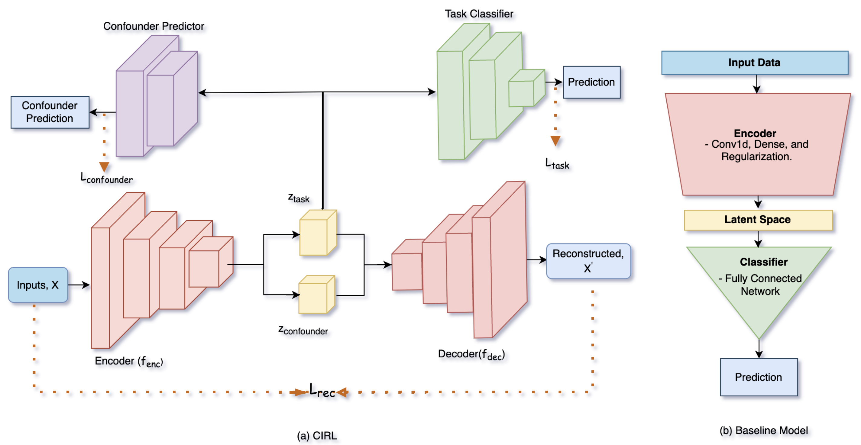
The CIRL model is a disentangled autoencoder that learns two distinct latent representations from input aroma data , where represents the domain of time-series or tabular sensor responses (e.g., 32-channel impedance data from the Noze Aroma Chip). The architecture is structured to separate task-relevant features (e.g., VOC identities) from confounders (e.g., humidity), ensuring robustness in data-scarce regimes.
The encoder, , maps the input data into two latent spaces: , where and denote the dimensions of the task-relevant and confounding latent spaces, respectively. The architecture of adapts based on the data type, for aroma data the temporal convolutional layers or recurrent models encode sequential information.
The decoder, , reconstructs the input data: , with a reconstruction loss ensuring . The decoder typically mirrors the encoder’s structure to ensure symmetry in feature representation.
The confounder predictor enforces invariance by predicting confounding attributes: where C denotes the confounding factors such as environmental variables or demographic attributes. Similarly, the task-specific classifier predicts task labels: where y represents task-specific outcomes.
Figure 1.
(a) Overview of the proposed disentangled autoencoder (CIRL) architecture. The input data X is passed through the encoder , which generates two disentangled latent representations: and . These representations are used by the decoder for reconstruction, on the other had used by the task classifier and confounder predictor for their respective outputs. The overall training is governed by the loss functions , , and , combined into .(b) The architecture of the baseline model we used to compare with, which contains same encoder and classifier as CIRL.
Figure 1.
(a) Overview of the proposed disentangled autoencoder (CIRL) architecture. The input data X is passed through the encoder , which generates two disentangled latent representations: and . These representations are used by the decoder for reconstruction, on the other had used by the task classifier and confounder predictor for their respective outputs. The overall training is governed by the loss functions , , and , combined into .(b) The architecture of the baseline model we used to compare with, which contains same encoder and classifier as CIRL.
4.2. Loss Functions
The CIRL framework optimizes three interdependent loss functions to enforce disentanglement and task performance. These losses—Reconstruction Loss , Task Loss , and Confounder Loss —create a balanced optimization landscape, akin to a minimax game in adversarial training. This interdependence ensures that the model learns representations that are both informative for the task and invariant to confounders, while maintaining fidelity to the input data:
Reconstruction Loss (): Ensures that the decoder accurately reconstructs the input data from the latent representations:
where is a loss function appropriate to the data type, e.g., Mean Squared Error (MSE) for aroma data.
Task Loss (): Ensures that retains the features relevant to the primary task:
e.g. can be binary cross-entropy for classification.
Confounder Loss (): Ensures that is invariant to the confounding attributes:
e.g. using MSE for continuous confounders like humidity.
The Total Loss () combines these components with hyperparameters , , and :
The negative sign on introduces an adversarial dynamic, while the confounder predictor h minimizes to accurately predict C from , the encoder maximizes it to make invariant. This opposes the cooperative minimization of and creating an equilibrium-like balance during training. From an information perspective (aligned with the Information Bottleneck principle), the losses optimize a trade-off: and maximizes mutual information to retain data fidelity and relevance respectively. On the other hand, minimizes mutual information for invariance.
4.3. Hyperparameter Tuning
The hyperparameters , , and govern the balance between reconstruction fidelity, task performance, and confounder invariance in the CIRL framework, critical for robust digital olfaction applications under confounding factors like humidity. Tuning these parameters requires careful consideration of their impact on e-nose datasets where high humidity obscures subtle VOC signals.
- The parameter emphasizes reconstruction fidelity, where a higher weight (e.g., 1.0–2.0) ensures accurate reconstruction of sensor signals. However overemphasis risks retaining humidity information in , reducing humidity-invariance representation.
- The parameter controls the importance of learning task-relevant attributes, and hence underweighting it can lead to poor task performance.
- The parameter encourages learning humidity-invariant attributes alongside retaining task-relevant information, however, setting it to an excessive weight (e.g. ) may disrupt task-relevant attribute encoding.
A hyperparameter search method (e.g. Grid Search, Bayesian Hyperparameter Optimization) is employed to explore the hyperparameter space using an exhaustive search. Dynamic adjustment leverages loss gradients to guide hyperparameter updates, expressed as . Validation-based thresholding ensures that validation metrics determine acceptable ranges for reconstruction fidelity, task performance, and invariance.
4.4. Implementation Considerations
The CIRL architecture is modular, adapting to aroma data types (e.g., time-series) with configurable encoder-decoder pairs. Training stability is ensured with gradient clipping (threshold 1.0) to prevent exploding gradients during adversarial steps. Evaluation metrics include reconstruction accuracy (e.g. root mean squared error, RMSE) and task performance (e.g. F1-score), computed on validation splits.
| Algorithm 1 Training Procedure for CIRL |
|
5. Sensors, Devices and Datasets
The methods presented in this paper are specifically designed to learn confounding invariant representation of data collected for a digital olfaction technology developed at Noze Inc. Noze’s aroma chip has affinity towards water and hence the humidity variations in the introduced aroma sample is a confounding factor for interpreting the aroma. First, the aroma chip was used to build digital nose device prototypes in several form factors which were used to capture (breath) aroma datasets in environments where the induced confounders’ specific variance, particularly humidity, interferes with learning generalizable task-specific patterns over the data. In this section, we introduce the aroma chip, the digital nose prototype devices and the aroma sampling process we used for the data collection. Subsequently we describe an overview of the specific aroma datasets that were used for the machine learning experiments. In the next section, we demonstrate the utility of CIRL in mitigating the generalizability challenges induced by the humidity confounder.
5.1. Aroma Sensor and Digital Nose Prototypes
The Noze aroma chip forms the foundation of the Noze digital olfaction platform. To facilitate the aroma sampling process for a given aroma sensing application, tailor made digital nose prototype devices were developed for (i) capturing the target aroma sample and (ii) introducing the aroma sample to the aroma chip’s headspace. For most applications, the aroma sampling process is an episodic process with 3 phases - phase 1 is introducing the ambient environment onto the aroma chip’s headspace which serves as the baseline. Phase 2 is replacing the baseline sample in the headspace with the aroma sample and during Phase 3 the ambient baseline is once again introduced to replace the aroma sample. During these 3 phases, the changes in aroma composition are recorded as changes in impedance characteristics across the 32 sensing elements.
5.1.1. The Noze Aroma Chip
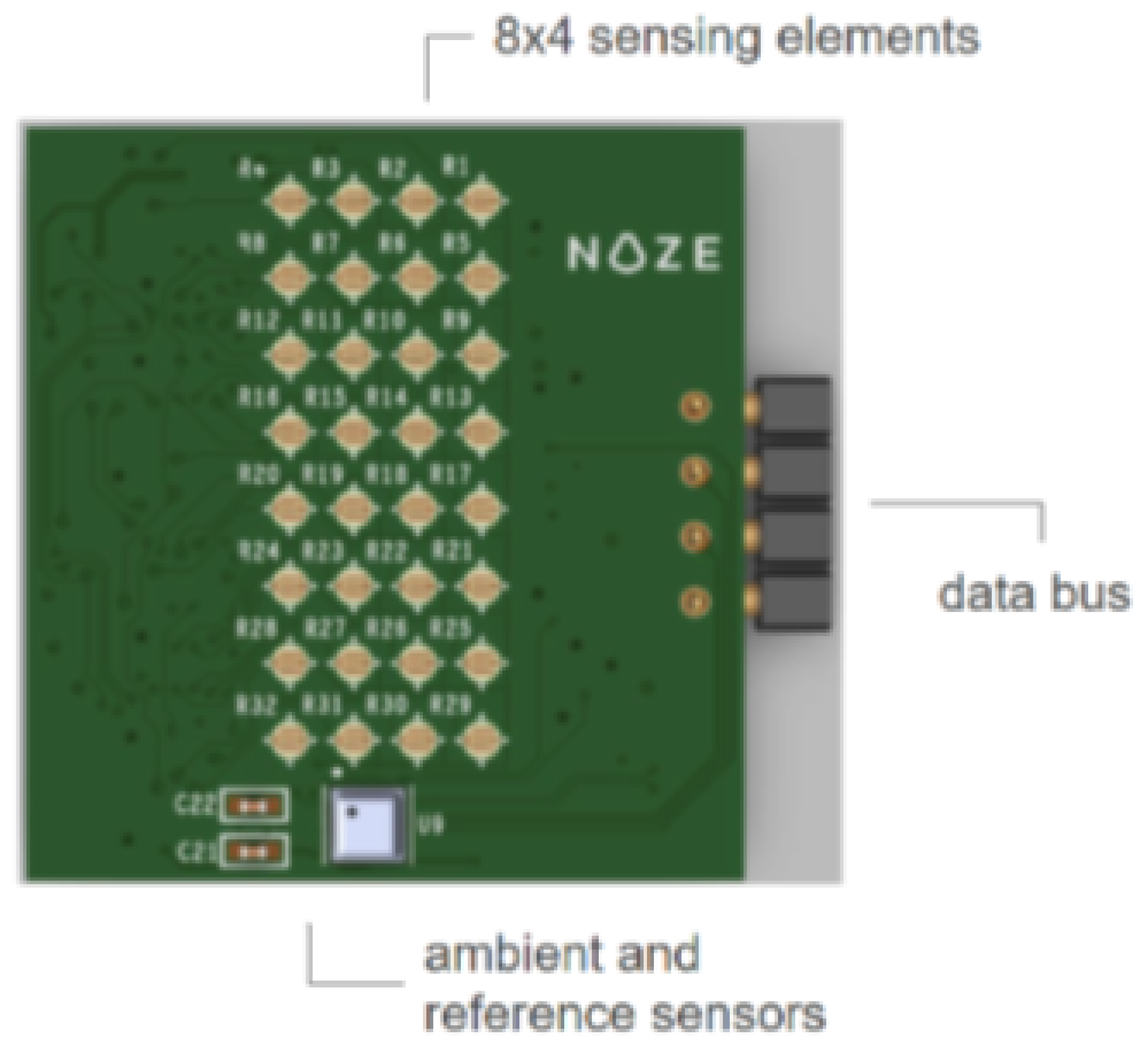
The aroma chip consists of (i) 32 thin film sensing elements, , (ii) reference and ambient sensors, and (iii) a data acquisition mechanism to enable a measurement circuit to read the data.. Each thin film is a unique nanocomposite material designed and characterized for affinity in room temperature towards a certain group of VOCs. Exposure of the thin film array to VOC molecules changes their impedances that are measured digitally. The readout circuit measures the impedance changes at a sampling rate of 1Hz. The engineered semi-selective sensing elements in the thin film array, captures the aroma information via temporal dynamics over the 32 dimensional time-series. For the ambient sensing, we used an off-the-shelf sensor (BME688).
Figure 2.
Noze’s proprietary sensor, featuring an array of 32 sensing elements configured as thin films.
Figure 2.
Noze’s proprietary sensor, featuring an array of 32 sensing elements configured as thin films.
Noze’s digital nose prototype shown below in Figure 3 has three key elements. (1) The aroma chip, (2) the chip enclosure that serves as a headspace and (3) a pump that performs active sampling of the aroma.. The pump pulls the aroma sample into the headspace and lets the sample percolate for the aroma chip to react and generate the fingerprint.
5.1.2. A Vial Based Aroma Sampler
Another device configuration that we developed leverages the digital nose prototype for digitizing the aroma samples prepared in 20mL glass vials. The setup as shown in Figure 4 consists of a digital nose unit on top, pulling the aroma sample from the vial through a 5mm PTFE tube as the sampler’s head. Once the aroma samples are prepared in the vials, the sampler’s head goes inside the vial headspace to sample the aroma. The sampling protocol consists of (i) baseline phase: 30 seconds of sampling air from the ambient as a reference gas, then (ii) aroma introduction phase: 30 seconds of sampling the vial’s headspace, followed by (iii) recovery phase: 50 seconds of sampling air from the ambient again.
5.1.3. The DiagNozeTM Breathalyzer Device
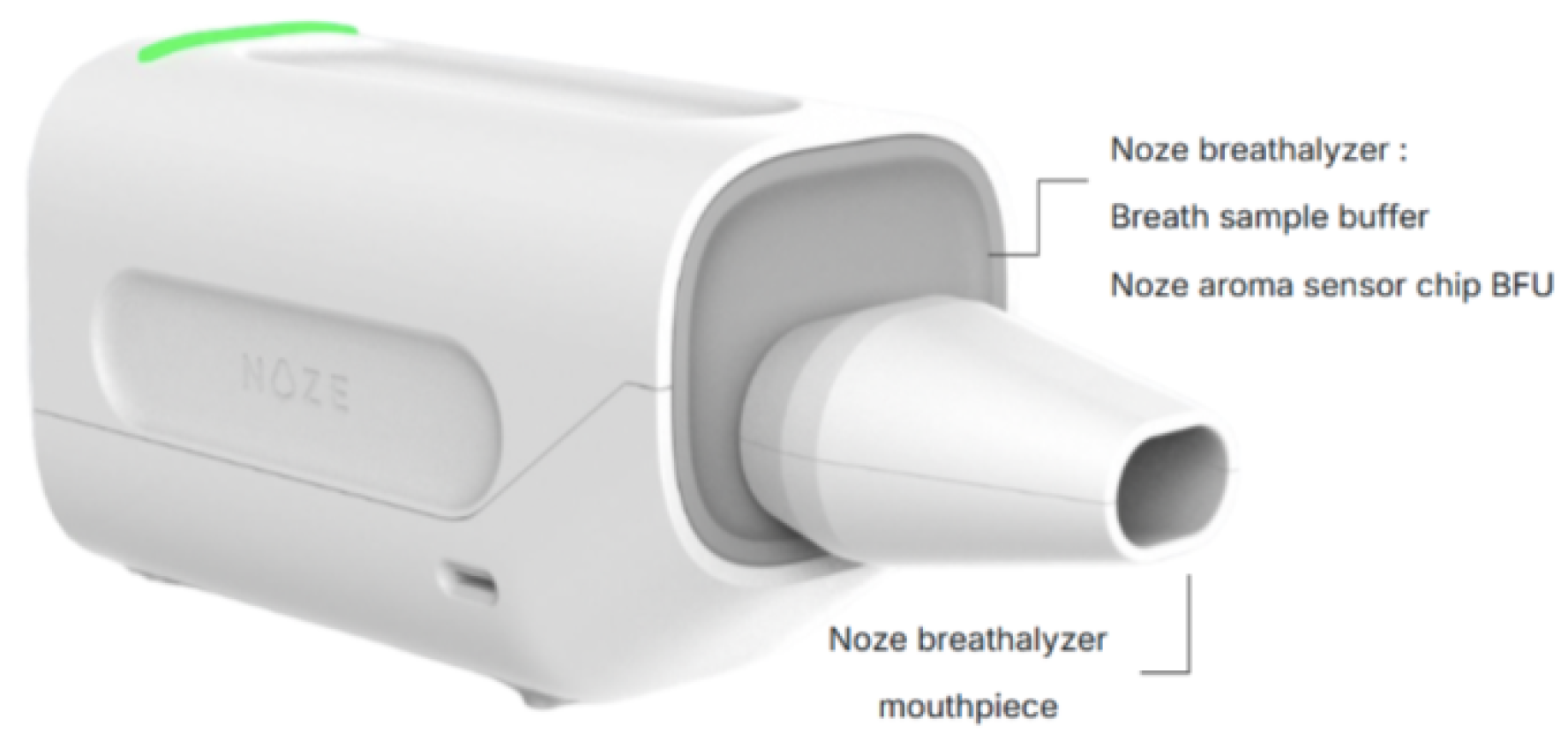
The DiagNozeTM Breathalyzer device integrates the digital nose unit in a breath sampling module to detect VOCs in exhaled breath. Participants exhale into a detachable, single patient use mouthpiece fitted with a microbial filter, humidity filter, and backflow prevention valve for safety. The breath sampling module has a capnography valve which allows only the alveolar portion—enriched with metabolic VOCs—into an internal buffer chamber which is then directed to the digital nose unit for digitization into an aroma fingerprint.
Figure 5.
DiagNozeTM breathalyzer device with the detachable mouthpiece.
5.2. Aroma Digitization Protocols
The aroma digitization protocol includes three steps, for (i) establishing an ambient aroma reference, (ii) the absorption phase, (iii) the desorption phase
- Baseline Phase: Prior to introducing the aroma sample to the sensor, the sensor measures the ambient environment using filtered air to establish a stable reference.
- Aroma Sampling Phase: Aroma sample gets introduced and adsorbed onto the sensing elements.
- Recovery Phase: The aroma molecules desorb from the sensing elements and revert to the baseline state.
The responses of the sensing elements of the aroma chip during each phase is reflective of the sensing elements characteristic and their interaction with the molecular composition they are exposed to.
5.3. Aroma Datasets
To assess the model’s efficacy in real-world scenarios, we assembled three aroma datasets from the aforementioned device prototypes. A prevalent challenge across these datasets is humidity’s confounding effect, as the aroma sensor is sensitive to humidity. Human exhaled breath harbors high humidity levels (∼30,000–50,000 ppm), creating a dominant background signal that obscures trace VOC fingerprints and hinders robust model development for mapping sensor outputs to target compounds.
5.3.1. Acetone Aroma Dataset
This dataset includes 385 digitized aroma samples of acetone at varying concentrations, collected via the Vial Aroma Device. Acetone’s elevated vapor pressure relative to water facilitates rapid volatilization into the humidity-saturated vial headspace. Sensors respond to both acetone and humidity, allowing evaluation of methods for acetone quantification amid confounding water signals. The samples are distributed across six distinct concentration levels—0 µL, 5 µL, 10 µL, 20 µL, 50 µL, and 100 µL of acetone dissolved in 10 mL of water—with approximately 65 samples per level.
5.3.2. Ketosis Breath Aroma Dataset
Comprising 168 digitized breath samples from an individual across four ketogenic diet cycles [35], this dataset categorizes breath ketone levels as low (≤10 ppm; 112 samples) or high (≥20 ppm; 56 samples). In high-ketosis states, breath ketones (20–70 ppm) are dwarfed by water vapor. Distinguishing subtle signal differences amid high background humidity poses a machine learning challenge, exacerbated by dataset imbalance and size.
5.3.3. Peppermint-Oil Breath Aroma Dataset
This dataset encompasses 361 breath samples from 19 participants: 191 pre-ingestion and 170 post-ingestion of a peppermint oil capsule. Post-ingestion, VOCs such as menthone and menthol are exhaled at 10–200 ppb. Detecting these traces is impeded by humidity responses, with dataset variability and size further complicating generalizable model development [36].

Table 1.
Summary of Aroma Datasets Used in the Study.
| Dataset | Total Samples | Classes/Concentrations | Key Challenge | Source Device |
| Acetone Aroma | 385 | 6 levels (0–100 L acetone) | Humidity confounding acetone signals | Vial-based aroma sampler |
| Ketosis Breath Aroma | 168 | Low-ketone (112); High-ketone (56) | Subtle ketone signals vs. high humidity; imbalance | DiagNozeTM Breathalyzer |
| Peppermint-Oil Breath Aroma | 361 | Pre-ingestion (191); Post-ingestion (170) | Trace VOC detection amid humidity; variability | DiagNozeTM Breathalyzer |
6. Experimental Evaluation
Building on the sensors, devices, and datasets described in the previous section, we conducted targeted experiments to quantify CIRL’s effectiveness in disentangling confounders from task-relevant features. Each experiment compares a baseline model—lacking explicit disentanglement mechanisms—against CIRL, which employs structured latent spaces for VOCs and humidity. We simulated realistic confounding scenarios to highlight CIRL’s improvements in reconstruction fidelity, confounder mitigation, and classification accuracy. Training utilized Adam optimization across all models, with hyperparameters tuned for fairness. Performance metrics, including mean squared error (MSE) for reconstruction and binary cross-entropy for classification, were evaluated on held-out test sets to ensure generalizability.
6.1. Acetone Aroma Experiment
This experiment assesses disentanglement in controlled acetone concentration classification amid humidity confounding.The baseline model unifies the encoder and latent space for classification, compressing inputs into a single latent vector fed to a classifier with fully connected and Conv1D layers, batch normalization, and LeakyReLU activation. It minimizes categorical cross-entropy loss without adversarial or reconstruction components (learning rate: , decay: 0.95 every 500 steps). Lacking confounder mitigation, it serves as a reference for entanglement effects.
In contrast, CIRL employs a disentangled autoencoder separating VOC and humidity latent spaces. These spaces support (1) input reconstruction, (2) humidity prediction, and (3) VOC-based classification. The training objective combines weighted reconstruction, classification, and adversarial confounder losses, with feature variances informing reconstruction weights and ensuring VOC representations remain independent of humidity. By enforcing humidity independence in VOC representations, CIRL enhances robustness over the baseline.
6.2. Ketosis Breath Aroma Experiment
Focusing on binary classification of ketone levels in breath samples, this experiment addresses subtle signal detection against high humidity backgrounds. The baseline is a CNN with stacked Conv1D layers, batch normalization, ReLU activation, and pooling, compressing features into a latent vector for classification via binary cross-entropy loss. Without disentangling humidity, it risks feature entanglement. CIRL introduces distinct latent spaces: VOC for classification-relevant features and humidity for confounders. A decoder reconstructs inputs from both, a humidity predictor estimates confounders, and a label predictor classifies via VOC space. Training minimizes reconstruction loss (MSE), classification loss (binary cross-entropy), and adversarial loss for invariance, using Adam optimization. This decoupling yields superior robustness.
6.3. Peppermint-Oil Breath Aroma Experiment
This binary classification task evaluates trace VOC detection pre- and post-peppermint ingestion, complicated by humidity and inter-participant variability.The baseline uses stacked Conv1D layers with batch normalization, ReLU, and pooling for feature extraction into a single latent space, performing classification via binary cross-entropy loss. Confounders remain entangled without isolation mechanisms.
CIRL structures latent spaces for VOC (task-relevant) and humidity (confounding), with a decoder for reconstruction, a humidity predictor, and a VOC-based classifier. Multi-objective training minimizes reconstruction, classification, and adversarial losses (learning rate: , Adam optimizer). Explicit disentanglement improves prediction robustness compared to the baseline.
6.4. Results and Observation
Our proposed method consistently and significantly outperformed the baseline models across all binary classification tasks. As presented in Table 2 and Table 3, a clear and compelling improvement in F1-score is evident for every class. The proposed method demonstrated improvements across all metrics, indicating its ability to effectively disentangle task-relevant features from confounding noise. The improved F1-scores for all classes confirm that the overall accuracy of our proposed method is superior to that of the baseline.
Overall, CIRL demonstrates superior generalization capabilities, with improvements observed across all challenging datasets. We observed gains for traditionally difficult classes within the Acetone Aroma Dataset, such as C2 and C3, as well as better performance on the Ketosis Breath Dataset and Peppermint-Oil Breath Dataset, all of which underscore its exceptional handling of complex tasks and confounding variables.
7. Conclusions
This work introduces a disentangled autoencoder framework that effectively bridges the gap between invariant and disentangled representation learning. Our approach achieves a crucial goal for artificial olfaction: the separation of task-relevant chemical features from confounding factors. Through evaluations on both synthetic and real-world aroma datasets, particularly those influenced by environmental distortions like humidity variations, our proposed architecture demonstrates better performance in generalization, reconstruction fidelity, and task accuracy when compared to standard baseline approaches. The framework yields consistent improvements in both binary and multiclass classification accuracy, along with substantial gains in F1-scores across diverse aroma sensing tasks. Importantly, it exhibits remarkable resilience to prevalent confounders in digital olfaction applications, such as sensor noise, domain shifts, and critical environmental factors like relative humidity. By explicitly modelling these confounding factors and enforcing task-specific invariance through adversarial learning, our model produces interpretable latent representations of chemical signals. This structured disentanglement not only ensures better task performance but also minimizes the influence of spurious correlations introduced by environmental variables. Furthermore, the versatility of our framework is notable. It readily supports the integration of regressors for predicting continuous task-specific outcomes, such as chemical concentrations, alongside or instead of classifiers. This dual capability allows the model to address a broad spectrum of prediction tasks within the same adaptable architecture. The design of this disentangled autoencoder seamlessly integrates with various aroma data modalities, including time-series responses from sensor arrays, making it a powerful tool for real-world digital olfaction applications where confounding influences are prevalent and reliable analysis is paramount. Overall, this work significantly advances the state-of-the-art in feature-invariant representation learning for artificial olfaction. It provides a robust, interpretable, and highly adaptable framework with the strong potential to enhance the reliability and scalability of digital olfaction systems across diverse industrial, environmental, and biomedical domains. Future research will explore further extensions of this framework, including dynamic loss scaling for enhanced training stability, adaptive disentanglement strategies for novel confounder detection, and its deployment in real-time digital olfaction applications within highly challenging and dynamic environments.
8. Future Works
Future research in disentangled representation learning should focus on improving loss balancing, adaptive latent spaces, and broader applicability. A key direction is dynamically adjusting reconstruction, task, and invariance losses during training, ensuring optimal trade-offs. Meta-learning or reinforcement-based optimization could fine-tune loss weights in real time, enhancing stability and performance. Additionally, dynamically scaling latent space dimensionality based on data complexity and confounding strength could improve model flexibility. Neural architecture search or information-theoretic constraints could help optimize representation capacity while maintaining interpretability. Expanding the framework to handle both classification and regression tasks simultaneously would increase its versatility across domains like healthcare, finance, and autonomous systems. Establishing standardized bench-marks using a semi-supervised approach with real-world confounded datasets and robust disentanglement metrics would facilitate fair comparisons and enhance reproducibility. By addressing these challenges, CIRL can evolve into a powerful tool for mitigating confounding influences, improving generalization, and advancing deep learning models in diverse applications.
Author Contributions
Conceptualization, Ashok Prabhu Masilamani, Mojtaba Khomami Abadi and Md Hafizur Rahman.; methodology, Mojtaba Khomami Abadi and Md Hafizur Rahman.; software, Alaa Wardeh. and Jayden K. Hooper; validation, Mojtaba Khomami Abadi. and Md Hafizur Rahman.; formal analysis, Md Hafizur Rahman; investigation, Md Hafizur Rahman.; data curation, Alaa Wardeh.; writing—original draft preparation, Md Hafizur Rahman.; writing—review and editing, Ashok Prabhu Masilamani and Mojtaba Khomami Abadi.; supervision, Mojtaba Khomami Abadi.; project administration, Mojtaba Khomami Abadi.;. All authors have read and agreed to the published version of the manuscript.
Funding
This research received no external funding.
Acknowledgments
During the preparation of this manuscript, the authors used Gemini 2.5 Pro for the purposes of grammar checking and polishing the texts . The authors have reviewed and edited the output of Gemini 2.5 Pro and take full responsibility for the content of this publication
Conflicts of Interest
The authors declare no conflicts of interest.
References
- Loutfi, A.; Coradeschi, S.; Mani, G.K.; Shankar, P.; Rayappan, J.B.B. Electronic noses for food quality: A review. Journal of Food Engineering 2015, 144, 103–111. [Google Scholar] [CrossRef]
- Wilson, A.D. Future Applications of Electronic-Nose Technologies in Healthcare and Biomedicine. In Wide Spectra of Quality Control; Akyar, I., Ed.; IntechOpen: Rijeka, 2011. [Google Scholar] [CrossRef]
- Robbiani, S.; Lotesoriere, B.J.; Dellacà, R.L.; Capelli, L. Physical Confounding Factors Affecting Gas Sensors Response: A Review on Effects and Compensation Strategies for Electronic Nose Applications. Chemosensors 2023, 11. [Google Scholar] [CrossRef]
- Abdullah, A.N.; Kamarudin, K.; Kamarudin, L.M.; Adom, A.H.; Mamduh, S.M.; Mohd Juffry, Z.H.; Bennetts, V.H. Correction Model for Metal Oxide Sensor Drift Caused by Ambient Temperature and Humidity. Sensors 2022, 22. [Google Scholar] [CrossRef]
- Nandy, A.; Duan, C.; Kulik, H.J. Audacity of huge: overcoming challenges of data scarcity and data quality for machine learning in computational materials discovery. Current Opinion in Chemical Engineering 2022, 36, 100778. [Google Scholar] [CrossRef]
- Kingma, D.P.; Welling, M. Auto-Encoding Variational Bayes. 2022, arXiv:stat.ML/1312.6114. [Google Scholar] [PubMed]
- Higgins, I.; Matthey, L.; Pal, A.; Burgess, C.P.; Glorot, X.; Botvinick, M.M.; Mohamed, S.; Lerchner, A. beta-vae: Learning basic visual concepts with a constrained variational framework. ICLR (Poster) 2017, 3. [Google Scholar]
- Ganin, Y.; Ustinova, E.; Ajakan, H.; Germain, P.; Larochelle, H.; Laviolette, F.; March, M.; Lempitsky, V. Domain-adversarial training of neural networks. Journal of machine learning research 2016, 17, 1–35. [Google Scholar]
- Jia, Z.; Patra, A.; Kutty, V.K.; Venkatesan, T. Critical Review of Volatile Organic Compound Analysis in Breath and In Vitro Cell Culture for Detection of Lung Cancer. Metabolites 2019, 9. [Google Scholar] [CrossRef]
- Hamaguchi, R.; Sakurada, K.; Nakamura, R. Rare event detection using disentangled representation learning. In Proceedings of the Proceedings of the IEEE/CVF Conference on Computer Vision and Pattern Recognition, 2019, pp.
- Locatello, F.; Bauer, S.; Lucic, M.; Rätsch, G.; Gelly, S.; Schölkopf, B.; Bachem, O. Challenging Common Assumptions in the Unsupervised Learning of Disentangled Representations. 2019, arXiv:1811.12359. [Google Scholar] [CrossRef]
- Rezende, D.; Mohamed, S. Variational inference with normalizing flows. In Proceedings of the International conference on machine learning. PMLR; 2015; pp. 1530–1538. [Google Scholar]
- Sanchez, E.H.; Serrurier, M.; Ortner, M. Learning disentangled representations via mutual information estimation. In Proceedings of the Computer Vision–ECCV 2020: 16th European Conference, Proceedings, Part XXII 16. Glasgow, UK, August 23–28, 2020; Springer, 2020; pp. 205–221. [Google Scholar]
- Hjelm, R.D.; Fedorov, A.; Lavoie-Marchildon, S.; Grewal, K.; Bachman, P.; Trischler, A.; Bengio, Y. Learning deep representations by mutual information estimation and maximization. 2019, arXiv:1808.06670. [Google Scholar] [CrossRef]
- Higgins, I.; Matthey, L.; Pal, A.; Burgess, C.; Glorot, X.; Botvinick, M.; Mohamed, S.; Lerchner, A. beta-VAE: Learning Basic Visual Concepts with a Constrained Variational Framework. In Proceedings of the International Conference on Learning Representations; 2017. [Google Scholar]
- Denton, E.L.; et al. Unsupervised learning of disentangled representations from video. Advances in neural information processing systems 2017, 30. [Google Scholar]
- Villegas, R.; Yang, J.; Hong, S.; Lin, X.; Lee, H. Decomposing motion and content for natural video sequence prediction. arXiv preprint 2017, arXiv:1706.08033 2017. [Google Scholar]
- Mathieu, M.; Couprie, C.; LeCun, Y. Deep multi-scale video prediction beyond mean square error. 2016, arXiv:1511.05440. [Google Scholar] [CrossRef]
- Park, S.; Kim, D.; Hwang, S.; Byun, H. Readme: Representation learning by fairness-aware disentangling method. arXiv preprint 2020, arXiv:2007.03775 2020. [Google Scholar]
- Wu, A.; Liu, R.; Han, Y.; Zhu, L.; Yang, Y. Vector-decomposed disentanglement for domain-invariant object detection. In Proceedings of the Proceedings of the IEEE/CVF International Conference on Computer Vision; 2021; pp. 9342–9351. [Google Scholar]
- Do, K.; Tran, T. Theory and evaluation metrics for learning disentangled representations. arXiv preprint 2019, arXiv:1908.09961 2019. [Google Scholar]
- Ganin, Y.; Lempitsky, V. Unsupervised domain adaptation by backpropagation. In Proceedings of the International conference on machine learning. PMLR; 2015; pp. 1180–1189. [Google Scholar]
- Peng, X.; Huang, Z.; Sun, X.; Saenko, K. Domain agnostic learning with disentangled representations. In Proceedings of the International conference on machine learning. PMLR; 2019; pp. 5102–5112. [Google Scholar]
- Cheng, H.; Wang, Y.; Li, H.; Kot, A.C.; Wen, B. Disentangled feature representation for few-shot image classification. IEEE transactions on neural networks and learning systems 2023. [Google Scholar] [CrossRef]
- Zhang, B.H.; Lemoine, B.; Mitchell, M. Mitigating unwanted biases with adversarial learning. In Proceedings of the Proceedings of the 2018 AAAI/ACM Conference on AI, Ethics, and Society; 2018; pp. 335–340. [Google Scholar]
- Arjovsky, M.; Bottou, L.; Gulrajani, I.; Lopez-Paz, D. Invariant Risk Minimization. 2020, arXiv:stat.ML/1907.02893. [Google Scholar]
- Bousmalis, K.; Trigeorgis, G.; Silberman, N.; Krishnan, D.; Erhan, D. Domain Separation Networks. 2016, arXiv:1608.06019. [Google Scholar] [CrossRef]
- Louizos, C.; Swersky, K.; Li, Y.; Welling, M.; Zemel, R. The Variational Fair Autoencoder. 2017, arXiv:1511.00830. [Google Scholar] [CrossRef]
- Khemakhem, I.; Kingma, D.; Monti, R.; Hyvarinen, A. Variational Autoencoders and Nonlinear ICA: A Unifying Framework. In Proceedings of the Proceedings of the Twenty Third International Conference on Artificial Intelligence and Statistics, 26–28 Aug 2020; Chiappa, S., Calandra, R., Eds.; PMLR; Vol. 108, Proceedings of Machine Learning Research. pp. 2207–2217. [Google Scholar]
- Achille, A.; Soatto, S. Emergence of invariance and disentanglement in deep representations. The Journal of Machine Learning Research 2018, 19, 1947–1980. [Google Scholar]
- Cover, T.; Thomas, J. Elements of information theory; Wiley-Interscience, 2006. [Google Scholar]
- Tishby, N.; Pereira, F.C.; Bialek, W. The information bottleneck method. 2000, arXiv:physics.data-an/physics/0004057. [Google Scholar] [PubMed]
- Vapnik, V.N. Statistical Learning Theory. Wiley-Interscience, 1998. [Google Scholar]
- Mohri, M.; Rostamizadeh, A.; Talwalkar, A. Foundations of Machine Learning, 2nd ed.; The MIT Press, 2018. [Google Scholar]
- Ketogenic diet. Wikipedia; accessed 02-September-2025.
- Henderson, B.; Ruszkiewicz, D.M.; Wilkinson, M.; Beauchamp, J.D.; Cristescu, S.M.; Fowler, S.J.; Salman, D.; Francesco, F.D.; Koppen, G.; Langejürgen, J.; et al. A benchmarking protocol for breath analysis: the peppermint experiment. Journal of Breath Research 2020, 14, 046008. [Google Scholar] [CrossRef] [PubMed]
Figure 3.
Noze digital nose prototype is designed to control the flow dynamics of the aroma sample over the aroma sensor chip.
Figure 3.
Noze digital nose prototype is designed to control the flow dynamics of the aroma sample over the aroma sensor chip.
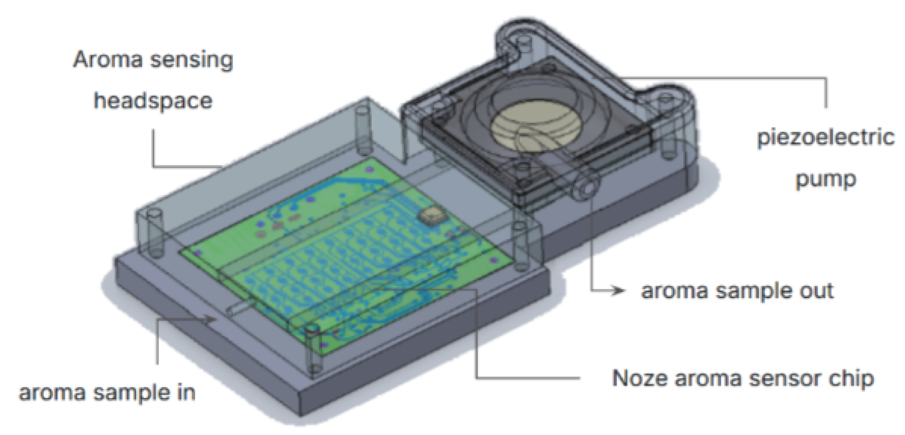
Figure 4.
A vial-based aroma sampler system in which the aroma sensor unit pulls the aroma from an aroma vial sample.
Figure 4.
A vial-based aroma sampler system in which the aroma sensor unit pulls the aroma from an aroma vial sample.
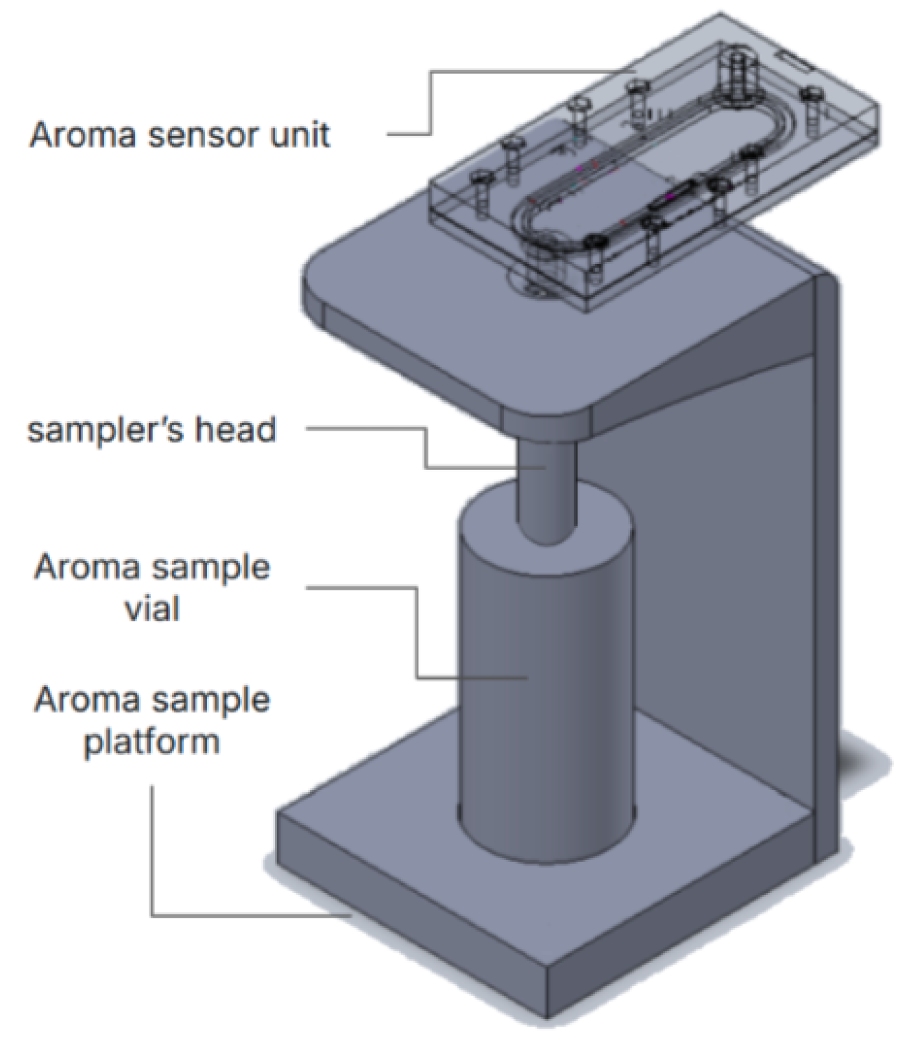
Table 2.
This table compares the class-specific F1-scores of the baseline model and CIRL on the acetone aroma dataset across blind test splits. CIRL achieves an average 15% improvement in F1 scores. Notably, its ability to distinguish water aroma samples from those with low acetone content improves by 24% in class F1-score. Each class corresponds to the injected acetone volume in 10mL of water during aroma digitization.
Table 2.
This table compares the class-specific F1-scores of the baseline model and CIRL on the acetone aroma dataset across blind test splits. CIRL achieves an average 15% improvement in F1 scores. Notably, its ability to distinguish water aroma samples from those with low acetone content improves by 24% in class F1-score. Each class corresponds to the injected acetone volume in 10mL of water during aroma digitization.
| acetone volume | baseline F1-score | CIRL F1-score |
| 0 L | 0.62 | 0.86 |
| 5 L | 0.55 | 0.67 |
| 10 L | 0.47 | 0.63 |
| 20 L | 0.68 | 0.73 |
| 50 L | 0.64 | 0.80 |
| 100 L | 0.58 | 0.82 |
Table 3.
The table compares the baseline model with the CIRL model on the employed breath aroma datasets. For both peppermint-oil breath and ketosis breath datasets, the baseline model struggles to achieve an above-chance F1 score for detecting condition-specific VOCs in alveolar breath. In contrast, CIRL excels in identifying trace VOCs within the complex background of human breath. This advancement paves the way for developing generalizable semantic representations of trace breath VOCs, resilient to known confounding factors.
Table 3.
The table compares the baseline model with the CIRL model on the employed breath aroma datasets. For both peppermint-oil breath and ketosis breath datasets, the baseline model struggles to achieve an above-chance F1 score for detecting condition-specific VOCs in alveolar breath. In contrast, CIRL excels in identifying trace VOCs within the complex background of human breath. This advancement paves the way for developing generalizable semantic representations of trace breath VOCs, resilient to known confounding factors.
| breath aroma classes | baseline vs CIRL F1-score |
| pre peppermint-oil intake | 0.51 vs 0.74 |
| post peppermint-oil intake | 0.38 vs 0.74 |
| low ketosis | 0.78 vs 0.93 |
| high ketosis | 0.42 vs 0.88 |
Disclaimer/Publisher’s Note: The statements, opinions and data contained in all publications are solely those of the individual author(s) and contributor(s) and not of MDPI and/or the editor(s). MDPI and/or the editor(s) disclaim responsibility for any injury to people or property resulting from any ideas, methods, instructions or products referred to in the content. |
© 2025 by the authors. Licensee MDPI, Basel, Switzerland. This article is an open access article distributed under the terms and conditions of the Creative Commons Attribution (CC BY) license (http://creativecommons.org/licenses/by/4.0/).
Copyright: This open access article is published under a Creative Commons CC BY 4.0 license, which permit the free download, distribution, and reuse, provided that the author and preprint are cited in any reuse.