
Submitted:
04 September 2025
Posted:
05 September 2025
You are already at the latest version
Abstract
Time reversal techniques have been investigated for ultrasound and electromagnetic waves. It offers some advantages, particularly in cluttered and inhomogeneous environment, for point-to-point applications. The instrumentation usually employed for electromagnetic time-reversal involves costly vector network analyzers or different interconnected generators and receivers. This article explores the use of a commercial software-defined radio, in frequencies between 700 MHz and 2100 MHz, with indoor tests showing its performance and observed voltage gains for the received pulse.
Keywords:
inverse filtering
; focusing gain
; GNU radio
; software-defined radio
; time reversal
1. Introduction
The time-reversal (TR) technique for propagation was initially proposed for mechanical waves (ultrasound) [1] and later extended for electromagnetic fields [2], having been experimentally demonstrated in a reverberation chamber at the frequency of 2.45 GHz. When subject to a TR filter, waves are focused spatially and temporally on a specific point. Figure 1 shows an example of the complex environment where the TR technique can be of interest. The signal arriving at the receiver is a superposition of several attenuated and filtered copies of the transmitted pulse, in general without a distinct line-of-sight (LOS), with the channel propagation following a Rayleigh model. TR helps focus the waves into the RX point, enabling a higher received amplitude at that specific local. It is, therefore, aimed at point-to-point operations.
The TR consists of basically two stages:
- Training: where a signal occupying the desired bandwidth B is transmitted and captured by the receiver, which in response develops a signal at its input, digitally recorded for the next step.
- TR: the received waveform is phase conjugated in frequency domain, , and retransmitted by the TX antenna. In the receiver, a signal develops on its terminals, which is expected to have a larger energy than the original . The relation between the amplitude of both signals is the gain parameter which expresses the advantage of the TR technique.
The phase conjugate wave is equivalent, in time domain, to a reverse time, flipping the time series that represent the received pulse. That has the effect of focusing the wave into that specific point. It benefits from very complex wireless channels, because all multipath rays contribute to the overall response [3]. Mathematically, the TR operation is equivalent to a pulse compression on the channel impulse response (CIR) , and the TR output resembles the response to an exciting pulse when has a large complexity [4], which in propagation terms implies a inhomogeneous and cluttered scenario. The operation is similar to a matched filter [5], and it is therefore akin to a retro-directive antenna array [6], which retransmits the signal back to the direction where the source is located. Concerning applications involving electromagnetic waves, TR has been reported to be used in communications [7], increasing the efficiency of wireless power transmission [8,9], in Radio-Frequency Identification systems (RFID) [10], ground-penetration radar enhancement [5], radar imaging [11], and also in Ultra-Wideband radar detection [4,12,13]. Specifically for RFID applications, a framework for simulating an environment using a 3D field solver was presented [14], where the whole virtual scenario was taken into account, including the RFID antennas. With the objective of alleviating the inter symbol interference (ISI) problem in a wireless system operating at 2.14 GHz, using a 10-MHz bandwidth and multiple input single output (MISO), a TR technique was used with better results in contrast to single-value decomposition (SVD) [15].
This article describes a TR setup using a software-design radio (SDR) as core instrument. Real-world implementations of TR used vector network analyzers (VNAs) [2,13], where the instrument high sensitivity and large bandwidth were exploited, and the measured signals sampled in the frequency domain were subjected to the TR mathematical operations elsewhere. Besides VNAs, a setup with oscilloscope, arbitrary waveform generator (AWG) and antennas [8,16] was employed. The different instruments demand a unique software control, usually Labview [17], to synchronize their operation and articulate the mathematical processing routines. SDRs, in turn, offer some benefits in relation to the other hardware items:
- Lower costs when compared to complex instrumentation like AWGs and VNAs.
- Open-source solutions to software control and integration.
- The software control interface has several built-in tools that help the TR flow design, such as filters, fast-fourier transform (FFT), decimators, etc.
- Seamless integration of software and hardware that enables a quick deployment of modifications, for instance, testing different frequencies, amplifier gains and transmitted power amplitudes.
- In case SDRs with two MIMO ports are employed, a complex signal is able to be retrieved (IQ samples), with information of phase.
- Lighter and with smaller dimensions.
As a downside, SDRs in general have narrower bandwidths in contrast to VNA’s and AWG’s, which limits the TR pulse width in frequency domain and therefore the overall scheme efficiency. SDRs operating with large instantaneous bandwidths (in excess of 100 MHz) are still costly.
This article describes tests with an SDR performing TR in an indoor environment. The used hardware (Section 2.1) and the software (Section 2.2) are described, with the procedures synthesized in the latter. Section 3 checks if the pulses delivered in time and frequency domains by the SDR are consistent, using a loopback configuration. Two indoor experiments are carried out in Section 4, with the respective gain results achieved by the TR technique.
2. Materials and Methods
2.1. Hardware
The software-defined radio NI USRP B210 [18] was employed for the tests. It covers the frequency range of 70 MHz to 6 GHz, and has four RF ports, which can be configured as multiple-input and multiple-output (MIMO). Each channel has a 12 bits analog-to-digital (ADC) and digital-to-analog converters (DAC), enabling a theoretical 74 dB signal to noise ratio (SNR). An internal Xilinx Spartan 6 XC6SLX150 FPGA controls the RF block, and it communicates with the host PC by means of a USB channel. For the RF part, a 15-cm telescopic-type wire monopole was used for the transmission, and a planar log-periodic antenna (LPDA) as receiver. The latter is directive whereas the former is omnidirectional, this choice justified by the possibility to orient the receiver antenna in directions other than facing the transmitter, so that a more complex propagation channel can be enforced. The SDR always operated with its maximum output power (16 dBm), confirmed after measurements with a spectrum analyzer. The B210, being MIMO-capable, has its ports locked into the same phase reference, making possible an IQ detection, where a complex signal is retrieved. In case one-port only SDR’s were used (e.g., Hack RF One, capable of operating as either transmitter or receiver, but in half-duplex mode), the measured signal would contain both IQ samples, but the phase part would be subjected to variations since the two devices (RX and TX) have their oscillators running freely and independently, without lock. Figure 2 shows the block diagram of the used hardware. Two of the four SDR ports are used, the other ones were left unconnected. The receiving antenna can be placed at distances up to 10 m away from the transmitter, by means of a coaxial cable.
In the USB port the SDR delivers a time-domain stream of complex numbers, occupying the baseband, alternating I and Q samples. The used application interface has to acquire these data and proceed with further tasks such as visualization and signal processing.
2.2. Software
GNU Radio [19] was used to interface with the SDR. It is an open-source framework, operating under the General Public License, and is used for interfacing with the SDR incoming data and performing signal processing and visualization functions. The final application, encapsulated as a Python file, can be run in a stand-alone fashion, or using the GNU Radio Companion, where the programming actually takes place with a block-oriented format. The same control and interface functions hereby used could have been implemented with Matlab [20] ou Labview [17], though they require paid licenses. Using the same B210 SDR with GNU Radio, a Digital TV 3.0-compatible ISDB-TB receiver was implemented, based on resources such as Low-Density Parity check (LDPC) codes, bit interleaving and Layer Division Multiplexing (LDM) [21]. In another reported example, different waveforms, e.g., orthogonal frequency division multiplexing (OFDM), triangular and sawtooth, were tested to check which one gave better performance for wireless power transfer [22].
The block diagram in the Figure 3 shows the final solution employed to integrate all the necessary TR steps. The pulse is formed with a Python application from two user inputs: the SDR sample rate and the desired pulse bandwidth B. A real-valued sequence of numbers, representing the pulse, is then passed to the GNU Radio Companion program, which is then transmitted by the TX antenna and received by the RX port, , after passing by the wireless channel. It is saved as a binary file. Once the training stage is performed, it is followed by the focusing stage. The stored train of received pulses is displayed by a Python code and the user selects two potential candidates to be used as the channel frequency response, based on their shape and amplitude. The Python code then outputs the time-reversal version of the channel response, the so-called pulse, which is radiated by the SDR port. For the sake of future comparisons, the original is also transmitted, so that the processing gain can be measured.
Preliminary tests were performed integrating more tasks in the GNU Radio, instead of using external Python programs. For instance, the pulse was first programmed using a block called Python snippet within the very GNU Radio Companion. However, due to hardware constraints imposed by the available laptop, it was decided to keep the GNU Radio application as lean as possible. Also, the Python offers better possibilities than GNU Radio to extract figures and debug the code. Both flowgraphs are shown in Figure 4, where the training program consists of the USRP reading a vector source and transmitting it, and the receiving channel receives the data from the antenna and saves it in a file (block named File Sink in the flowgraph). For the test, performance evaluations between the pulses is carried out by either transmitting one vector or another, which are input to the USRP sink as a vector source, imported from a Python code.
The pulse to be transmitted occupies a bandwidth B and is subjected to an SDR . It is interesting to note that the variable also describes the RF band centered on the central frequency . The pulse is then formed as:
where h is the Hamming window, the carrier frequency and the variable is defined as function of the SDR internal sample rate:
Following [10], the Hamming window multiplies the sinc function, to limit out-of-band emissions. The SDR operated with a sample rate of 25 MHz, and the pulse bandwidth was chosen to be 5 MHz and 10 MHz. The B210 unit reaches a maximum of 56 MHz, but this data rate has to be divided by two channels, 28 MHz. However, tests showed that a too-fast sample rate produced lost samples in the GNU Radio application, due to hardware (USB ports and processor overload) constraints. The pulse bandwidth B was then set to be slightly smaller than half of the sample rate parameter, so that the pulses can be adequately represented in time domain. Nevertheless, it has been observed in the literature that the TR gain improves with the pulse bandwidth B [23].
Once the pulse is synthesized by the Python code, it is transmitted as a train (every 20 ) and received by the antenna, - process carried out in the Training GNU Radio program. It is recorded and processed to generate the TR response, according to Figure 5. The next steps are followed in the Python code: First, two pulses (named A and B) are manually selected in the pulse train, they allow to choose which one has less noise and better performance. It also allows to compare their frequency domain shape, to see if they are similar. Then, a low-pass filter is applied to both pulses (Butterworth, order 12), to attenuate noise and out-of-band signals. Later, the two time series (Pulse A and B) are flipped and conjugated, to form the TR signal . One of them is chosen to be transmitted, based on its shape, amplitude and SNR.
The sequence of numbers is fed to the transmitter (represented by the USRP Sink in the diagram) by the vector source blocks, they are just copied and pasted from text files saved from the Python program. When they are fed as input to the USRP Sink block (Figure 4, Training), the waveform modulates the RF carrier , set by the user between 900 MHz and 2100 MHz, constraints set by the used antennas. Besides it, in the test program, both TR pulse and the training pulse are output, each one at a time, to evaluate their amplitudes squared on the received channel. It is important to stress that the energy of all pulses are normalized prior to the transmission, to enable fair amplitude comparisons in the receiving end. Its user interface is shown in Figure 6. That helps identify the received responses and measure their respective amplitudes, computing the gain.
Other parameters such as the frequency, the internal amplifier gain and the transmitted power were set by the user within the GNU Radio applications. As a final note, it was observed a better performance running the GNU Radio flowgraphs in an 8-GBytes RAM laptop with Ubuntu operational system (version 20.04.6) in comparison to 16-GBytes RAM laptop with Windows 10 - in terms of stability (GNU Radio crashes in the Win PC, when the program was terminated). More modern and powerful PC hardware would make the operation more stable regardless of GNU Radio parameters and the used operational system.
3. SDR Output Investigation
A preliminary test was carried out to check if the SDR hardware was able to output the desired pulse, since it might be too fast for its circuits and therefore transmitted with a deformed shape. In addition to an isolated pulse, all pulses within the train should maintain the same expected waveform, with a stable and predictable performance. Figure 7 contains the results for two received pulses randomly selected from the sequence, in contrast to the expected computed waveform, in both frequency and time domains. It can be seen that the curves in time comply reasonably well, though their power spectra shows that out-of-band emissions are larger than that expected from the theory. It justifies the use of a low-pass filter as shown in Section 2.2. The inset contains its basic measurement setup, with the SDR operated with its maximum output power and the RF input protected by means of a 30-dB attenuator.
It is interesting to stress that GNU Radio presents the plots in frequency domain with its own unit (dBr - relative dB), and not using the usual dBm, so a calibration is needed if actual quantities are to be shown. This procedure was performed using the SDR and GNU Radio connected to an RF generator and later compared to a spectrum analyzer, so a relation between dBr and dBm could be determined. During these evaluations it was also observed that the SDR internal amplifier gain (LNA) was not constant throughout the used frequency range, so this parameter had to be kept fixed during comparisons with different pulses and conditions.
4. Results
Different sets of experiments were carried out in order to address the effectivity of the TR technique using an SDR. One involved an indoor domestic environment, where other tests took place in a research laboratory, with larger distances.
4.1. Domestic Environment: Sweeping Frequency
The first evaluation was performed in a domestic environment, whose main dimensions are shown in Figure 8, with obstacles from furniture, domestic appliances, desktop computers, etc. The measured processing gain is defined following the model in [8]:
where both and are the time-domain received pulses of the transmitted TR and training signals, respectively, as shown pictorially in Figure 6. The magnitude squared is justified by the presence of complex signals, given the SDR IQ demodulation.
Since the received signal is actually a train of pulses, whose peak amplitudes vary in time, an average is computed in the QT GUI Number sink block, seen in Figure 4, bottom right corner. The test phase analyzes the received signal for both u and , and picks the maximum value after an observation time of 4 seconds.
For the test, both RX and TX antennas were kept fixed at the same positions throughout the whole experiment, while the central frequency was swept to analyze the its effect on the gain. Two different pulse bandwidths were tested, 10 MHz and 5 MHz, using a sample rate of 25 MHz. Each discrete frequency required its own training phase, given the dependency of the channel impulse response on the frequency. Results are shown in Figure 9. It is possible to see that gains are observed in all tested frequencies, with better performance around 1000 to 1200 MHz, for both pulse bandwidths. This peak can be ascribed to a better sensitivity, due to a combination of antennas, SDR frequency response and the channel itself.
To show the channel variation with frequency, it was measured with a vector network analyzer, keeping the same antennas and respective positions, the result is shown in Figure 10. Its frequency response is not flat, with multiple peaks in the S21 parameter, characteristic of multipath environment.
Ambient noise (Figure 11) was picked up in the majority of frequencies used in the test, since it was carried out in an urban area. Analyzing the train of pulses, the 900-MHz case contains a larger noise energy in contrast to 1300 MHz, as well the former peak amplitudes have wider amplitude fluctuation. That means the choice of an adequate pulse within the train is harder, due to the larger SNR.
Concerning output power level and the internal LNA gain, it was observed that for better performance, in terms of stability and repeatability, operating with maximum gain and maximum output power was preferred, otherwise fluctuations observed along the received train amplitude as well as the higher noise content jeopardized computing the gain.
4.2. Laboratory Environment: Computing the Gain for Different Positions
The other tests were carried out in a larger, more cluttered laboratory environment. Figure 12 shows the main dimensions of the area and its overall picture. Measurement results are summarized in Table 1. For each position, the transmitter was kept fixed and the receiving site was varied, and for that the training was performed and later the processing gain computed. The frequency of 1300 MHz was chosen to be used, given its good observed performance in the domestic environment. The sample rate was set to 25 MHz and the pulse bandwidth B to 10 MHz. Points (9) and (10) are in direct line-of-sight, with distances of respectively 5 and 2 meters from the transmitter.
From the results, one can see two interesting points: the largest gain was observed at point (2), where the receiver was placed right below a metallic equipment, in a very complex and harsh channel, as well as (8), where there was a wall between both spaces and a metallic table below the antenna. Also, the two LOS points had the situation of higher gain for the larger distance, where multiple reflections are likely to arise. Figure 13 shows the positions of these aforementioned spots.
The results confirm that the TR performs better when the filter is applied to a highly cluttered environment, with marginal gains for more homogeneous channels.
4.3. Gain for One Position and Addressing the Focusing at Other Untrained Points
The goal of this test was see how good the focusing took place for a specific point in space. This evaluation had the receiving and transmitter antenna trained for one spatial point, named target (chosen to be at position 8, with the metallic shield plates), and then the same gain was computed for untrained receiving positions other than the target. Throughout the whole procedure, the transmitter antenna was kept fixed. The receiving antennas were positioned on the same spots as depicted in Figure 12, and additional points were measured from the target, to see how the focusing behaves near the training spot took place. Also, two linearly spaced LOS spots were used. Results are presented in Table 2.
The results show again that whenever the propagation is clean, TR does not provide relevant advantages. Off-target (i.e., untrained) points provided moderate gains, and as the measured point moved away from the target, its gain has decreased, reaching even situations where the TR provided pulses with less energy than the original u. The target was also compared without the metallic plates, at the same position but in a less-complex propagation environment, and the gain also decreased, indicating that the presence of the obstacles impose a large difference on the channel impulse response, though the relative TX and RX positions were kept the same.
5. Conclusions
Realizing a TR experiment can be an involved task, since it deals with both RF and signal processing, as well as recording received signals to be later post processed. This work presented the use of a commercial software-defined radio with open-source applications, namely Python for signal processing and GNU Radio for hardware control. This combination resulted in a seamless and versatile TR system, easily reconfigured and debugged. Results originated from tests in two different indoor environments proved that the time reversal indeed provided energy gains and focusing, with better results for more complicated and inhomogeneous wireless channels.
Data Availability Statement
All data pertinent to this study is available upon request to the authors.
References
- Fink, M. Time Reversal of Ultrasonic Fields-Part Basic Principles. IEEE Trans. Ultrason., Ferroelectr., Freq. Control, 1992, 39, 555–588. [Google Scholar] [CrossRef] [PubMed]
- Lerosey, G.; de Rosny, J.; Tourin, A; Derode, A.; Montaldo, G.; Fink, M. Time reversal of electromagnetic waves. Phys. Rev. Lett., 2004, 92, 193904.
- Wu, F.; Fink, M. Time reversal of ultrasonic fields Part II: Experimental results. IEEE Trans. Ultrason., Ferroelectr., Freq. Control. 1992, 39, 567–578. [Google Scholar] [CrossRef] [PubMed]
- Sarkar, T. K.; Palma, M. S. Electromagnetic Time Reversal: What does it Imply? In 2016 URSI International Symposium on Electromagnetic Theory (EMTS), Espoo, Finland, 14–18 August 2016.
- Santos, V. R. N.; Teixeira, F. L. Application of time-reversal-based processing techniques to enhance detection of GPR targets. Journal of Applied Geophysics 2017, 146, 80–94. [Google Scholar] [CrossRef]
- Fusco, V.; Buchanan, N. Developments in retrodirective array technology. IET Microwaves, Antennas & Propagation 2013, 7, 131–140. [Google Scholar] [CrossRef]
- Khaleghi, A. Measurement and analysis of ultra-wideband time reversal for indoor propagation channels. Wireless Pers. Commun. 2010, 54, 307–320. [Google Scholar] [CrossRef]
- Ibrahim, R.; Voyer, D.; Bréard, A.; Huillery, J.; Vollaire, C.; Allard, B.; Zaatar, Y. Experiments of Time-Reversed Pulse Waves for Wireless Power Transmission in an Indoor Environment. IEEE Trans. Microw. Theory Techn. 2016, 64, 2159–2170. [Google Scholar] [CrossRef]
- Cangialosi, F.; Grover, T.; Healey, P.; Furman, T.; Simon, A.; Anlage, S. M. Time reversed electromagnetic wave propagation as a novel method of wireless power transfer. In 2016 IEEE Wireless Power Transfer Conference (WPTC), Aveiro, Portugal, 5–6 May 2016.
- Ezzeddine, H.; Merakeb, Y.; Huillery, J.; Bréard, A.; Duroc, Y. Pulsing the Passive RF Identification Technology. IEEE Microw. Magazine 2023, 24, 40–50. [Google Scholar] [CrossRef]
- Moura, J. M. F.; Jin, Y. Time Reversal Imaging by Adaptive Interference Canceling. IEEE Trans. Signal Processing. 2008, 56, 233–247. [Google Scholar] [CrossRef]
- Li, Y.; Xu, L.; Wang, P.; Ding, B.; Zhao, S.; Wang, Z. Ultra-Wideband Radar Detection Based on Target Response and Time Reversal. IEEE Sensors Journal. 2024, 24, 14750–14762. [Google Scholar] [CrossRef]
- Bellomo, L.; Belkebir, K.; Saillard, M.; Pioch, S.; Chaumet, P. Inverse Scattering Using a Time Reversal RADAR. In 2010 URSI International Symposium on Electromagnetic Theory, Berlin, Germany, 16–19 August 2010.
- Ezzedine, H.; Merakeby, Y.; Huillery, J.; Breard, A.; Duroc, Y.; Vollaire, C. Simulation Framework for Studying UHF RFID Systems in Pulse Wave Mode. In 2019 IEEE International Conference on RFID Technology and Applications (RFID-TA), Pisa, Italy, 25–27 September 2019.
- Nguyen, H. T.; Andersen, J. B.; Pedersen, G. F.; Kyritsi, P.; Eggers, P. C. F. Time reversal in wireless communications: a measurement-based investigation. IEEE Transactions on Wireless Communications. 2006, 5, 2242–2252. [Google Scholar] [CrossRef]
- Merakeb, Y.; Ezzeddine, H.; Huillery, J.; Bréard, A.; Touhami, R.; Duroc, Y. Experimental platform for waveform optimization in passive UHF RFID systems. RF and Microwave Computer Aided Engineering. 2020, 1–15. [Google Scholar] [CrossRef]
- https://www.ni.com/en.html. Available online: URL (accessed on 26 August 2025).
- https://www.ettus.com/all-products/ub210-kit/. Available online: URL (accessed on 26 August 2025). (accessed on null).
- http://gnuradio.org Available online: URL (accessed on 26 August 2025).
- https://www.mathworks.com/products/matlab.html Available online: URL (accessed on 26 August 2025).
- Rabaça, R. S.; de Oliveira, G. H. M. G.; Jerji, F.; Akamine, C. Implementation of a real-time ISDB-TB LDM receiver using SDR. In 2019 IEEE International Symposium on Broadband Multimedia Systems and Broadcasting (BMSB), Jeju, South Korea, 5–7 June 2019.
- Gautam, S.; Kumar, S.; Chatzinotas, S.; Ottersten, B. Experimental Evaluation of RF Waveform Designs for Wireless Power Transfer Using Software Defined Radio. IEEE Access. 2021, 9, 132609–132622. [Google Scholar] [CrossRef]
- Derode, A.; Touring, A.; Fink, M. Random multiple scattering of ultrasound. II. Is time reversal a self-averaging process? Phys. Rev. E. 2001, 64. [Google Scholar] [CrossRef] [PubMed]
- Author 1, T. The title of the cited article. Journal Abbreviation 2008, 10, 142–149. [Google Scholar]
- Author 2, L. The title of the cited contribution. In The Book Title; Editor 1, F., Editor 2, A., Eds.; Publishing House: City, Country, 2007; pp. 32–58.
- Author 1, A.; Author 2, B. Book Title, 3rd ed.; Publisher: Publisher Location, Country, 2008; pp. 154–196. [Google Scholar]
- Author 1, A.B.; Author 2, C. Title of Unpublished Work. Abbreviated Journal Name year, phrase indicating stage of publication (submitted; accepted; in press).
- Title of Site. Available online: URL (accessed on Day Month Year).
- Author 1, A.B.; Author 2, C.D.; Author 3, E.F. Title of presentation. In Proceedings of the Name of the Conference, Location of Conference, Country, Date of Conference (Day Month Year); Abstract Number (optional), Pagination (optional).
- Author 1, A.B. Title of Thesis. Level of Thesis, Degree-Granting University, Location of University, Date of Completion.
Figure 1.
Complex environments offer the large potential for the TR technique.
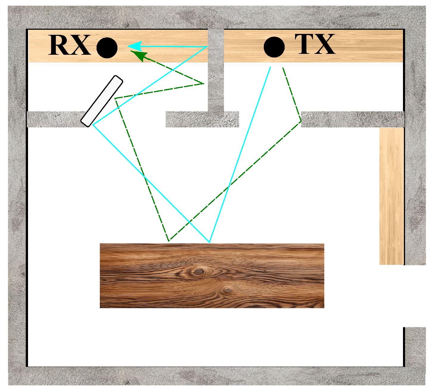
Figure 2.
Block diagram of the hardware.
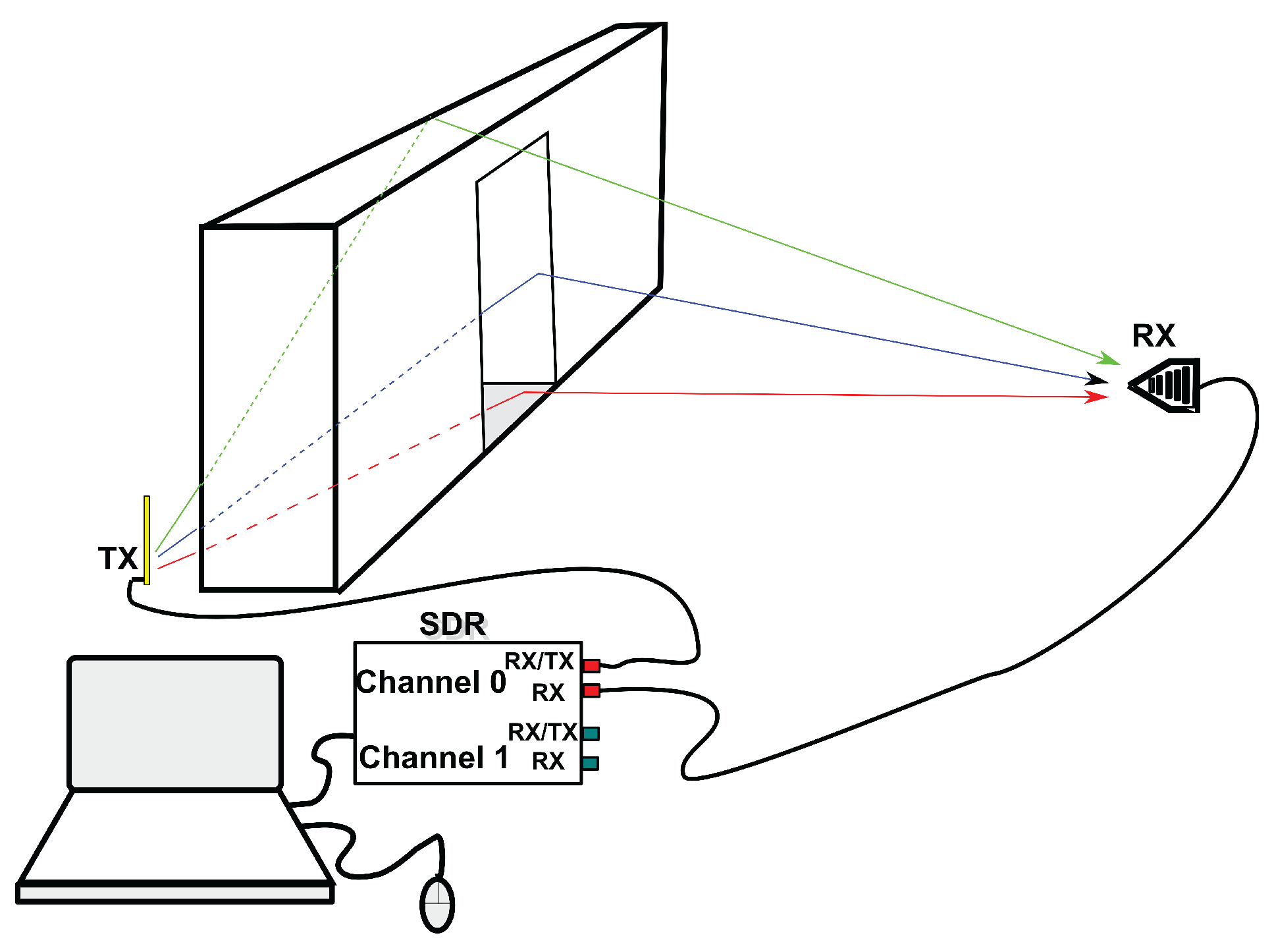
Figure 3.
Block diagram of the software applications and necessary steps.
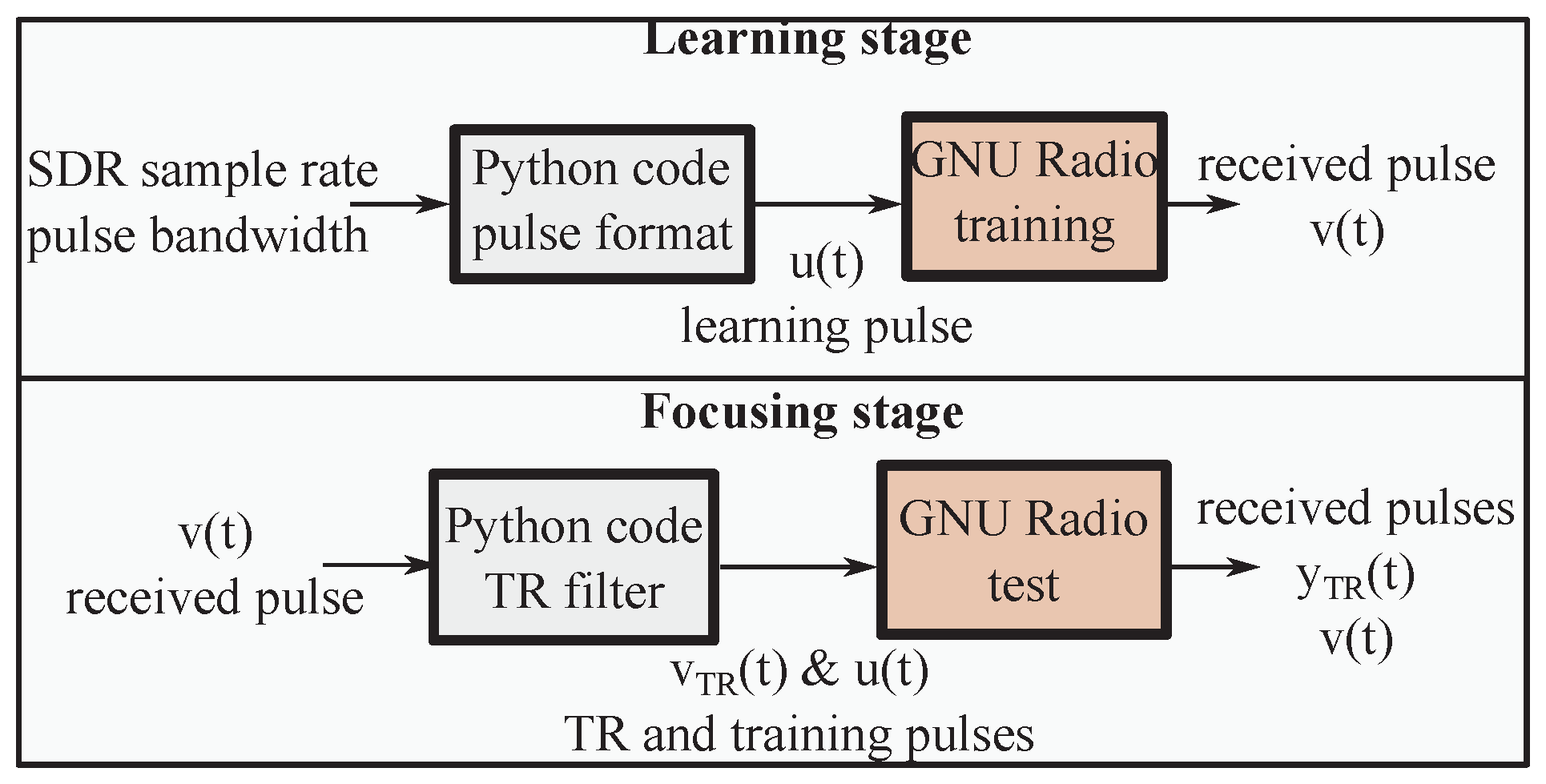
Figure 4.
GNU Radio Companion flowgraphs.
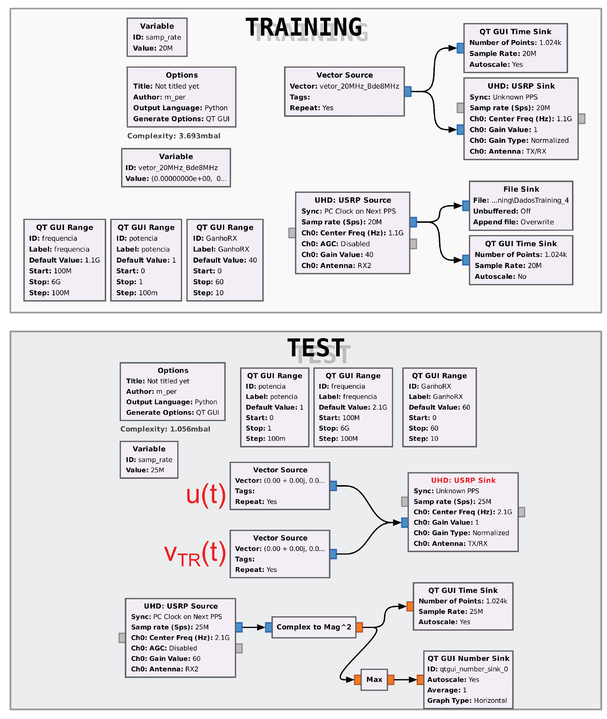
Figure 5.
Training steps. Two potential signals to be used are selected in (a), one of them is actually used. In (c), the power spectrum of the received pulses before and after filtering is shown with the original .
Figure 5.
Training steps. Two potential signals to be used are selected in (a), one of them is actually used. In (c), the power spectrum of the received pulses before and after filtering is shown with the original .
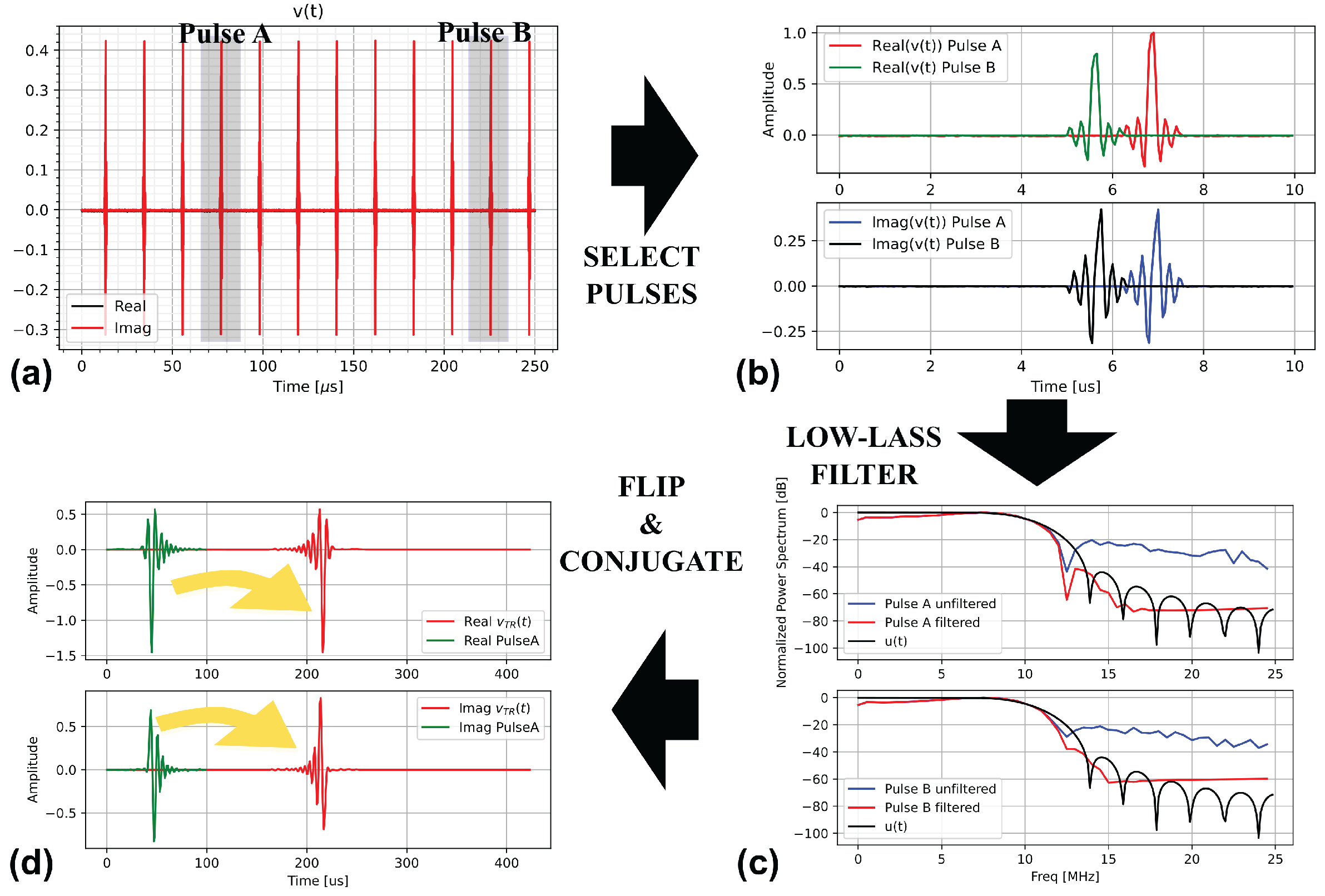
Figure 6.
Interface of the test application running the TR step.
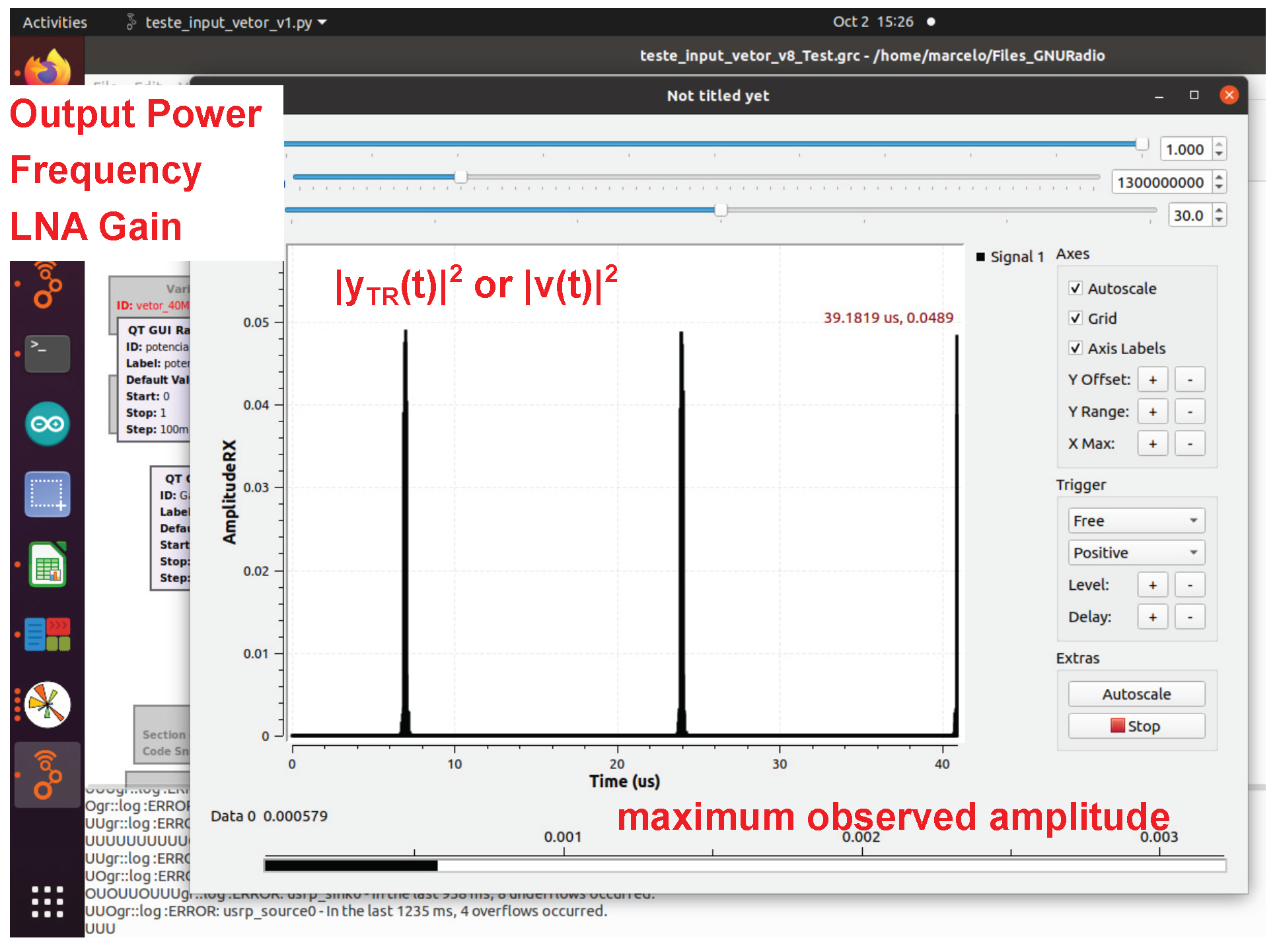
Figure 7.
Transmitted pulses (RX1 and RX2) compared to the mathematical expected shape, in time and frequency domains. Inset picture contains the setup used.
Figure 7.
Transmitted pulses (RX1 and RX2) compared to the mathematical expected shape, in time and frequency domains. Inset picture contains the setup used.
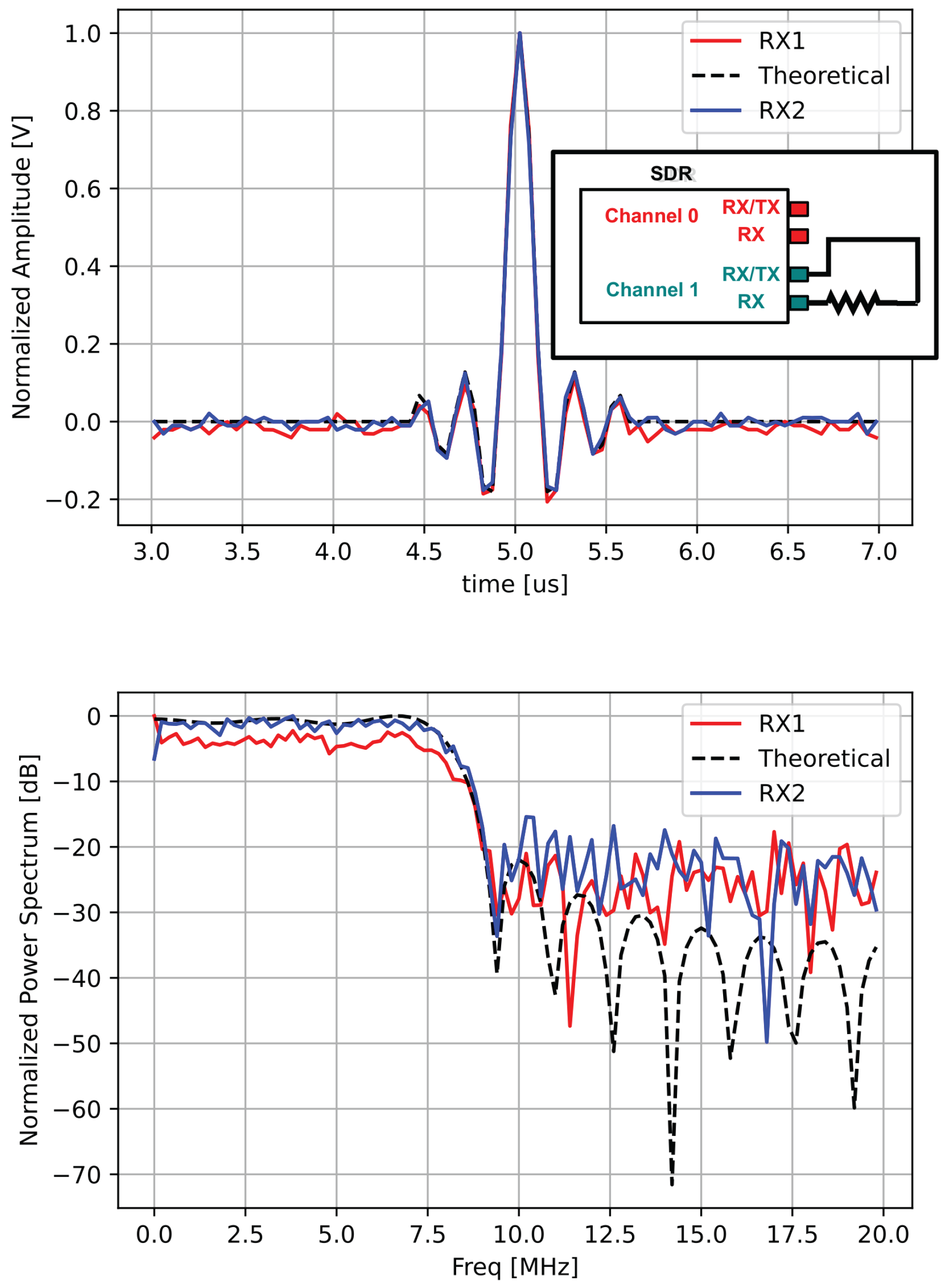
Figure 8.
Main dimensions (meters) of the TR test, domestic indoor environment.
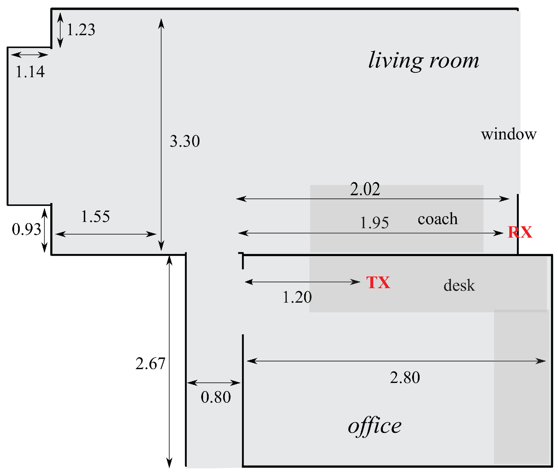
Figure 9.
Gain variation with different frequencies, for two pulse bandwidths.
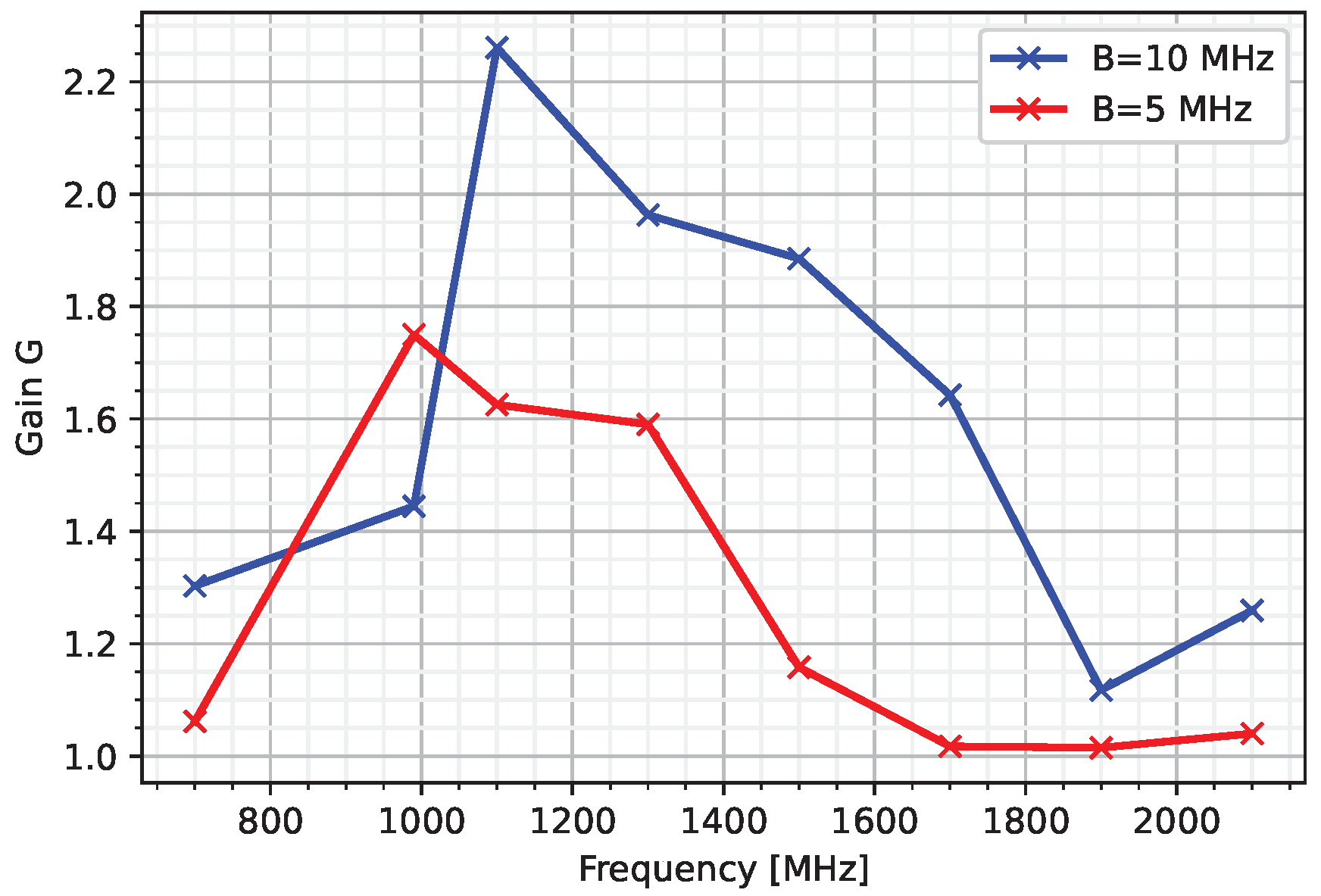
Figure 10.
Domestic channel Transfer function.
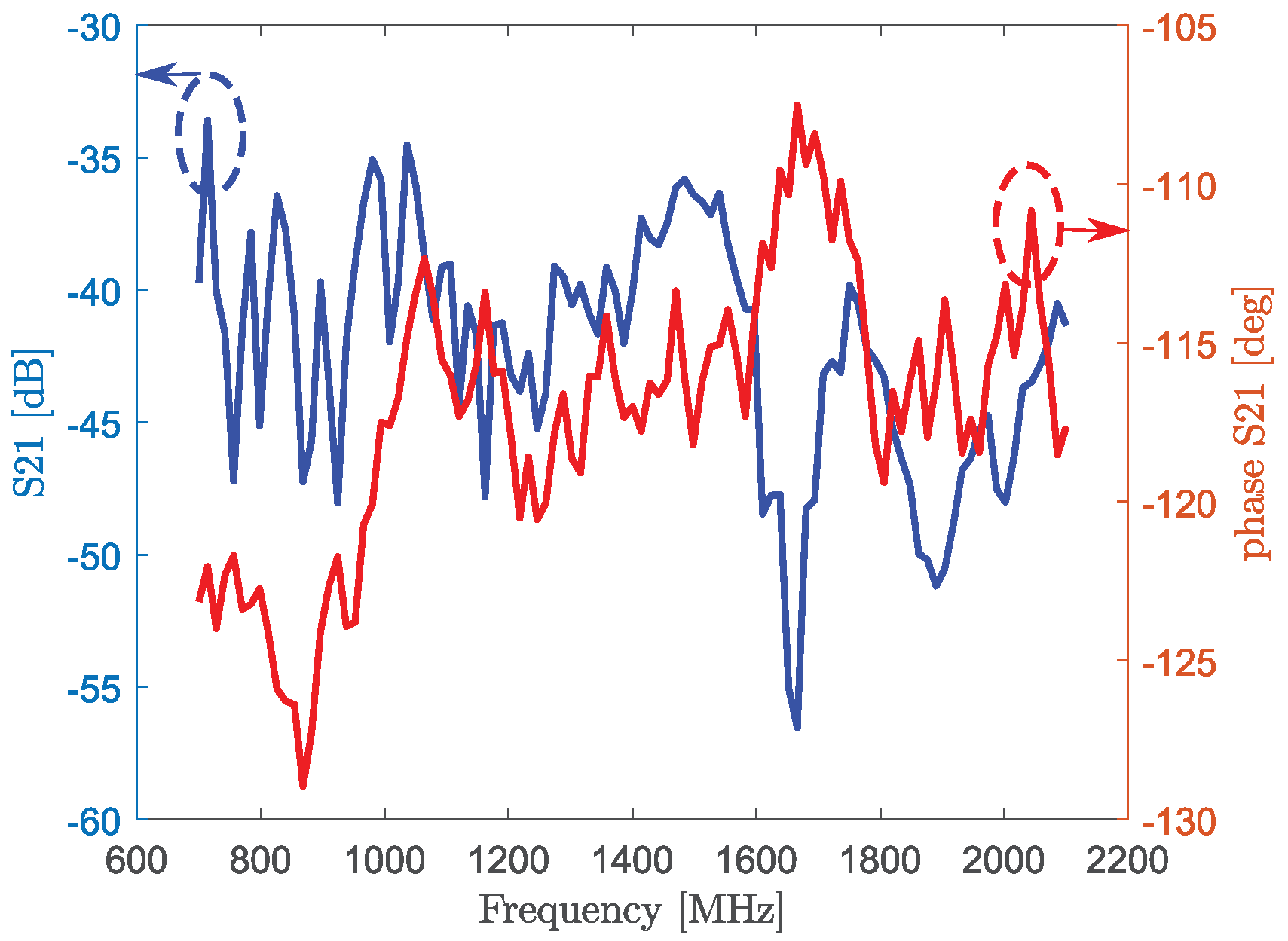
Figure 11.
Train of received pulses, for two different measured center frequencies.
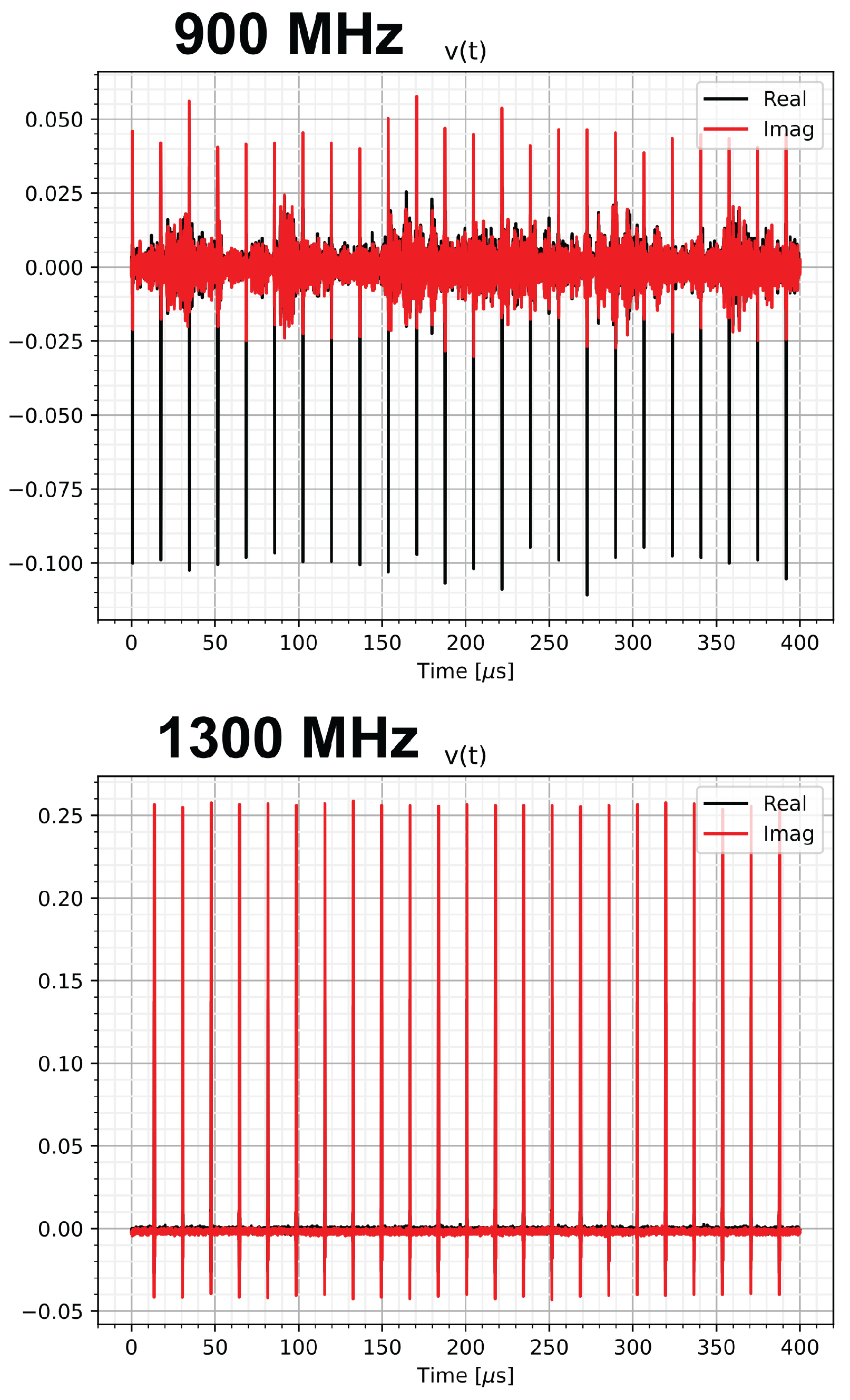
Figure 12.
Indoor dimensions (meters) with the measurement points, along with the actual environment picture.
Figure 12.
Indoor dimensions (meters) with the measurement points, along with the actual environment picture.
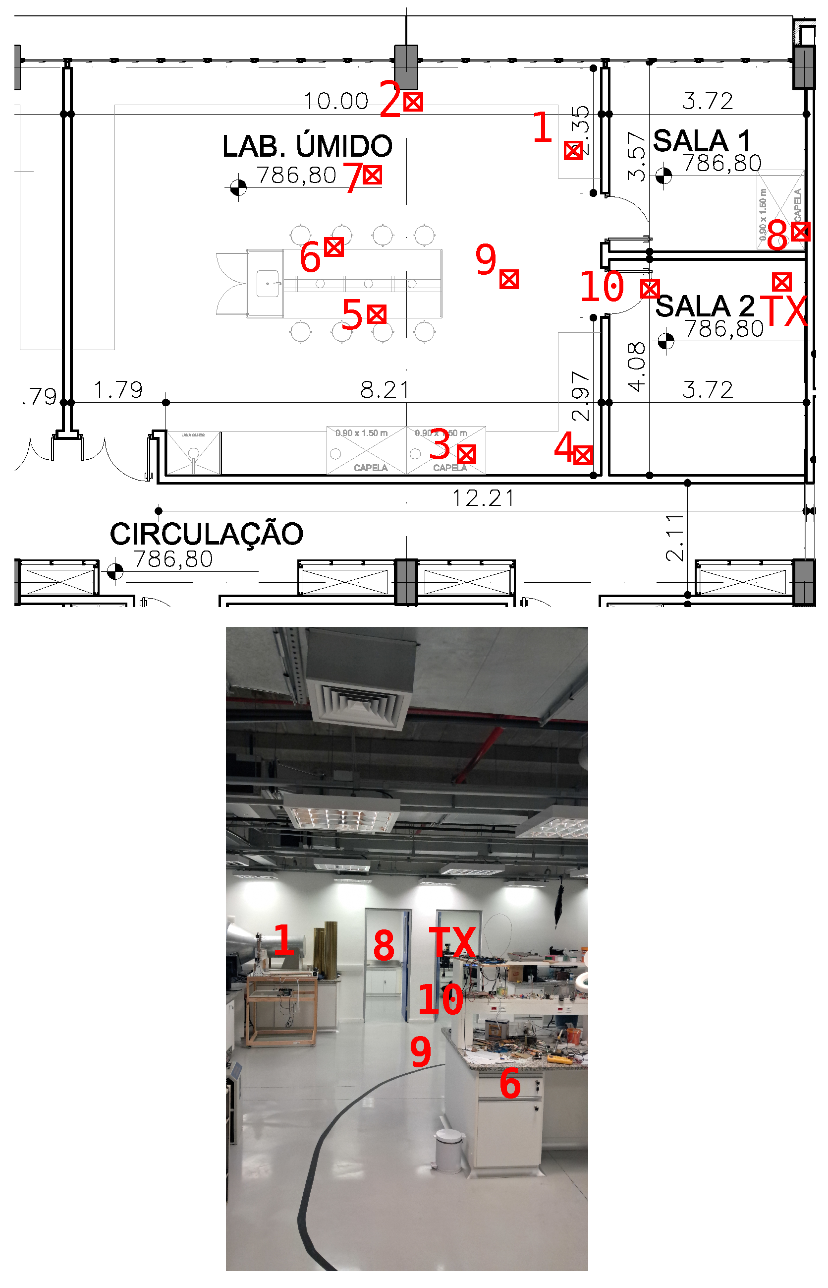
Figure 13.
Two different measured points, the (8) is seen with two metallic plates to create an artificial complex channel whereas the (9) has a LOS characteristics.
Figure 13.
Two different measured points, the (8) is seen with two metallic plates to create an artificial complex channel whereas the (9) has a LOS characteristics.
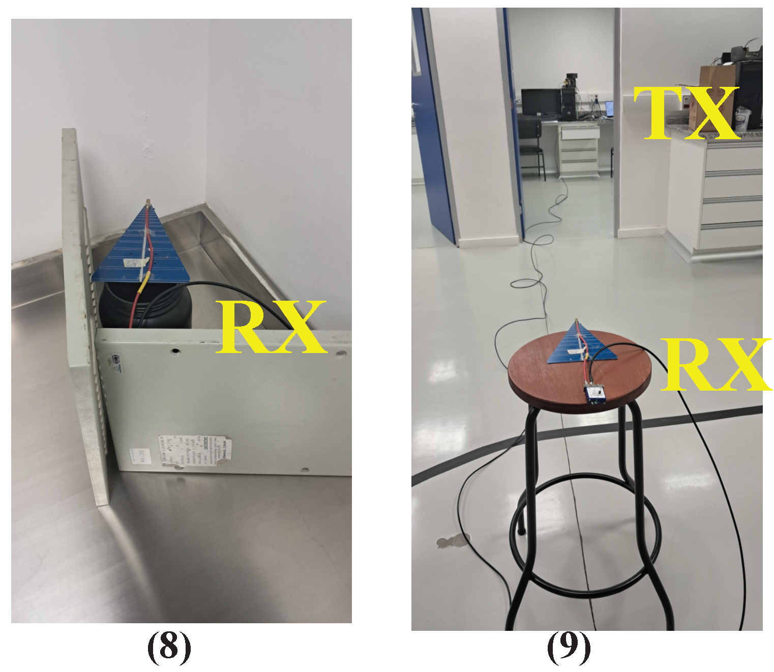

Table 1.
Gain for different positions
| Position | Gain |
|---|---|
| 1 | 2.43 |
| 2 | 3.82 |
| 3 | 2.00 |
| 4 | 1.69 |
| 5 | 1.91 |
| 6 | 2.08 |
| 7 | 2.07 |
| 8 | 2.18 |
| 9 | 3.32 |
| 10 | 2.17 |
Table 2.
Gain for positions other than the target
| Position | Gain |
|---|---|
| 1 | 1.32 |
| 2 | 1.02 |
| 3 | 0.97 |
| 4 | 0.90 |
| 5 | 1.00 |
| 6 | 1.01 |
| 7 | 1.22 |
| 8 (Trained target) | 2.10 |
| 8 (target) but without obstacles | 1.46 |
| 1 meter from 8 (target) | 1.16 |
| 2 meters from 8 (target) | 1.57 |
| LOS 3 m away | 0.49 |
| LOS 5 m away | 1.52 |
Disclaimer/Publisher’s Note: The statements, opinions and data contained in all publications are solely those of the individual author(s) and contributor(s) and not of MDPI and/or the editor(s). MDPI and/or the editor(s) disclaim responsibility for any injury to people or property resulting from any ideas, methods, instructions or products referred to in the content. |
© 2025 by the authors. Licensee MDPI, Basel, Switzerland. This article is an open access article distributed under the terms and conditions of the Creative Commons Attribution (CC BY) license (http://creativecommons.org/licenses/by/4.0/).
Copyright: This open access article is published under a Creative Commons CC BY 4.0 license, which permit the free download, distribution, and reuse, provided that the author and preprint are cited in any reuse.


