Submitted:
03 September 2025
Posted:
04 September 2025
You are already at the latest version
Abstract
The solution of partial differential equations (PDEs) underpins computational modeling across science and engineering, from quantum mechanics to climate dynamics. This review examines the current landscape of PDE solving methods, encompassing both traditional numerical approaches that have been refined over decades and emerging machine learning techniques that fundamentally transform computational paradigms. We systematically analyze classical methods, evaluating their mathematical foundations, computational characteristics, and fundamental limitations. The review then explores eleven major families of machine learning-based approaches: physics-informed neural networks, neural operators, graph neural networks, transformer architectures, generative models, hybrid methods, meta-learning frameworks, physics-enhanced deep surrogates, random feature methods, DeePoly framework, and specialized architectures. Through detailed comparative analysis of over 40 distinct ML methods, we assess performance across multiple dimensions, including computational complexity, accuracy bounds, multiscale capability, uncertainty quantification, and implementation requirements. Our critical evaluation reveals fundamental trade-offs: traditional methods excel in providing provable accuracy guarantees and rigorous error bounds, but face scaling challenges for high-dimensional problems; neural methods, on the other hand, provide unprecedented computational speed and flexibility, but lack rigorous error control and systematic uncertainty quantification. Hybrid approaches that combine physical constraints with learning capabilities are increasingly dominating the accuracy-efficiency frontier. We identify key challenges, including the absence of comprehensive theoretical frameworks for neural methods, limited software maturity, and the need for verification requirements in safety-critical applications. The review concludes by outlining future directions, including foundation models that demonstrate zero-shot generalization across PDE families, as well as quantum and neuromorphic computing paradigms, and automated scientific discovery. Rather than replacement, we advocate for synthesis: leveraging complementary strengths of traditional and machine learning methods to expand the frontier of computationally tractable problems. This integration promises to enable breakthrough capabilities in understanding and controlling complex physical systems, from molecular to planetary scales.
Keywords:
partial differential equations
; physics-informed neural networks
; neural operators
; computational mathematics
; foundation models
; numerical analysis
; scientific machine learning
; hybrid methods
1. Introduction
Partial differential equations (PDEs) constitute one of the most fundamental mathematical frameworks for describing natural phenomena across diverse scientific and engineering disciplines. From the fluid dynamics governing atmospheric circulation patterns [1,2] to the quantum mechanical wave functions describing atomic behavior [3,4], PDEs provide the mathematical language through which we model, understand, and predict complex systems. The ubiquity of PDEs in modern science stems from their ability to capture the spatial and temporal evolution of physical quantities, making them indispensable tools in physics, engineering, biology, finance, and numerous other fields.
The pervasive role of PDEs in scientific modeling cannot be overstated. In fluid dynamics, the Navier-Stokes equations govern the motion of viscous fluids [5,6], enabling the design of aircraft, the prediction of weather patterns, and the understanding of oceanic currents. Electromagnetic phenomena are elegantly described by Maxwell’s equations [7,8], which form the theoretical foundation for technologies ranging from wireless communications to magnetic resonance imaging. In biology, reaction-diffusion equations model pattern formation in developmental biology [9], tumor growth dynamics, and the spread of infectious diseases. Financial mathematics employs the Black-Scholes equation and its generalizations to price derivatives and manage risk in complex financial instruments [10]. Climate modeling relies on coupled systems of PDEs to simulate atmospheric and oceanic dynamics, providing crucial insights into global warming and extreme weather events [1,2].
The computational solution of these equations has become increasingly critical as scientific and engineering challenges grow in complexity and scale [11,12,13]. Modern applications often involve multi-physics phenomena, extreme parameter regimes, and high-dimensional parameter spaces that push traditional numerical methods to their limits [14,15,16]. This has sparked intense interest in developing new computational approaches, including machine learning-based methods that promise to overcome some of the fundamental limitations of classical PDE solving techniques.
The classification of PDEs provides essential insight into their mathematical structure and computational requirements. The fundamental categorization distinguishes between elliptic, parabolic, and hyperbolic equations based on the nature of their characteristic surfaces and the physical phenomena they describe [17,18].
Elliptic equations, exemplified by Laplace’s equation and Poisson’s equation , typically arise in steady-state problems where the solution represents an equilibrium configuration [19,20]. These equations exhibit no preferred direction of information propagation, and boundary conditions influence the solution throughout the entire domain. The canonical example is the electrostatic potential problem, where the potential at any point depends on the charge distribution throughout the entire domain and the boundary conditions [19,20]. Elliptic problems are characterized by smooth solutions in the interior of the domain, provided the boundary data and source terms are sufficiently regular [19,20].
Parabolic equations, with the heat equation serving as the prototypical example, describe diffusive processes evolving in time [21,22]. These equations exhibit a preferred temporal direction, with information propagating from initial conditions forward in time. The smoothing property of parabolic equations means that even discontinuous initial data typically evolve into smooth solutions for positive times [21,22]. Applications include heat conduction, chemical diffusion, and option pricing in mathematical finance. The computational challenge lies in maintaining stability and accuracy over long time intervals while respecting the physical constraint that information cannot propagate faster than the diffusion process allows [23,24,25].
Hyperbolic equations, including the wave equation and systems of conservation laws, govern wave propagation and transport phenomena [26,27]. These equations preserve the regularity of initial data, meaning that discontinuities or sharp gradients present initially will persist and propagate along characteristic curves [26,27]. The finite speed of information propagation in hyperbolic systems reflects fundamental physical principles such as the speed of light in electromagnetic waves or the speed of sound in acoustic phenomena [28,29]. Computational methods must carefully respect these characteristic directions to avoid nonphysical oscillations and maintain solution accuracy.
The distinction between linear and nonlinear PDEs profoundly impacts both their mathematical analysis and computational treatment [30,31]. Linear PDEs satisfy the superposition principle, allowing solutions to be constructed from linear combinations of simpler solutions [32,33]. This property enables powerful analytical techniques such as separation of variables, Green’s functions, and transform methods. Computationally, linear systems typically lead to sparse linear algebraic systems that can be solved efficiently using iterative methods [34].
Nonlinear PDEs, in contrast, exhibit far richer and more complex behavior. Solutions may develop singularities in finite time, multiple solutions may exist for the same boundary conditions, and small changes in parameters can lead to dramatically different solution behavior [30,31]. The Navier-Stokes equations exemplify these challenges, with phenomena such as turbulence representing complex nonlinear dynamics that remain elusive. Computationally, nonlinear PDEs require iterative solution procedures such as Newton’s method, often with sophisticated continuation and adaptive strategies to handle solution branches and bifurcations [30].
The proper specification of auxiliary conditions is crucial for ensuring well-posed PDE problems [17,35]. Boundary value problems involve specifying conditions on the spatial boundary of the domain [36]. Dirichlet boundary conditions prescribe the solution values directly, as in on . Neumann conditions specify the normal derivative, on , representing flux conditions in physical applications. Mixed or Robin boundary conditions combine both types, often arising in heat transfer problems with convective cooling. The choice of boundary conditions must be physically meaningful and mathematically appropriate for the PDE type.
Initial value problems specify the solution and possibly its time derivatives at an initial time. For first-order time-dependent PDEs, specifying suffices, while second-order equations like the wave equation require both and . The compatibility between initial and boundary conditions at corners and edges of the domain can significantly affect solution regularity and computational accuracy [37,38].
The evolution of numerical methods for PDEs reflects a continuous interplay between mathematical understanding, computational capabilities, and application demands. Traditional approaches, rooted in functional analysis and numerical linear algebra, have achieved remarkable success in solving a wide range of PDE problems. These methods, such as finite difference, finite element, and spectral methods, provide rigorous error estimates, conservation properties, and well-understood stability criteria [38,39,40,41]. However, they face significant challenges in high-dimensional problems due to the curse of dimensionality, struggle with complex geometries and moving boundaries, and often require extensive mesh generation and refinement strategies that can dominate the computational cost [42,43,44,45].
The emergence of machine learning approaches to PDE solving represents a paradigm shift in computational mathematics. Neural network-based methods, particularly physics-informed neural networks (PINNs) and deep operator learning frameworks, offer the potential to overcome some traditional limitations [15,45,46,47,48,49]. These approaches can naturally handle high-dimensional problems, provide mesh-free solutions, and learn from data to capture complex solution behaviors. However, they introduce new challenges related to training efficiency, solution accuracy guarantees, and the interpretation of learned representations [15,45,46,47,48,49]. The integration of physical constraints and conservation laws into machine learning architectures [50,51,52] remains an active area of research, with hybrid approaches that combine the strengths of traditional and machine learning methods [53,54,55] showing particular promise.
The present review aims to provide a state-of-the-art assessment of both traditional and machine learning methods for solving PDEs. We systematically examine the theoretical foundations, computational implementations, and practical applications of each approach. Throughout this review, we maintain a critical perspective, highlighting the strengths and limitations of each method and identifying open challenges that overcoming them may lead to more effective and efficient PDE solvers for the increasingly complex problems facing modern science and engineering.
2. Partial Differential Equations
2.1. Definition and Mathematical Formulation
A partial differential equation is a mathematical equation that relates a function of multiple variables to its partial derivatives. Formally, a PDE can be written as
where is the unknown function, represent the independent variables (typically spatial coordinates and time), and the equation involves partial derivatives up to some highest order k. The order of a PDE is determined by the highest-order derivative appearing in the equation.
PDEs can be systematically organized through a hierarchical classification framework. Figure 1 presents this taxonomy, beginning with order-based categorization and proceeding through type classification (elliptic, parabolic, hyperbolic) to linearity distinctions, ultimately connecting mathematical structure to physical applications and solution methodologies. This classification provides essential context for understanding the diverse approaches required across different PDE classes and their respective computational challenges.
PDEs serve as the mathematical language for describing continuous phenomena where quantities vary across space and time. Unlike ordinary differential equations (ODEs) [56] that describe evolution in a single variable, PDEs capture the multidimensional nature of physical fields, encoding local conservation principles and constitutive relations that govern macroscopic behavior. This fundamental capability makes PDEs indispensable for modeling systems where local interactions produce emergent global patterns.
The solution of a PDE is a function (for time-dependent problems) or (for steady-state problems) that satisfies the differential equation throughout a specified domain and meets prescribed auxiliary conditions [17,18]. The well-posedness of a PDE problem, in the sense of Hadamard, requires three fundamental properties [40,57]: existence (at least one solution exists), uniqueness (at most one solution exists), and continuous dependence on data (small perturbations in initial or boundary conditions lead to small changes in the solution). These properties ensure that PDE models provide physically meaningful and computationally stable predictions.
The formulation of mathematical models through PDEs represents a systematic methodology for encoding physical phenomena in mathematical structures. This process entails the identification of fundamental principles governing the system under consideration, followed by their translation into differential relations through appropriate mathematical frameworks. The governing principles emerge from the underlying physics of the problem, while their mathematical representation may be derived through infinitesimal analysis or variational formulations. The resulting differential equations must be complemented by auxiliary conditions that ensure well-posedness and reflect the specific configuration of the problem. This hierarchical construction—from physical principles to differential relations to complete boundary value problems—provides the foundation for both analytical investigation and computational solution of the modeled phenomena.
2.2. Theoretical Foundations
The mathematical theory underlying PDEs provides crucial insights into solution behavior, guiding both analytical understanding and computational methodology. This theoretical framework addresses fundamental questions about solutions’ existence, uniqueness, regularity, and qualitative properties [19,40,57,58].
The theoretical foundation of PDE analysis requires a systematic progression from physical modeling to rigorous mathematical formulation. Figure 2 illustrates this framework, showing how solution concepts generalize from classical to weak to distributional formulations, while the regularity ladder and embedding theorems provide the functional analytic tools necessary for establishing well-posedness and solution properties across different function spaces.
2.2.1. Existence and Uniqueness Theory
The existence of solutions to PDE problems is established through various mathematical frameworks, each suited to different equation types and solution concepts. For linear elliptic equations, the theory of weak solutions [19] has proven particularly powerful. Consider the abstract variational problem: find such that
where V is an appropriate Hilbert space, is a bilinear form, and is a linear functional. The Lax-Milgram theorem guarantees existence and uniqueness when is continuous and coercive, providing the theoretical foundation for finite element methods [59,60].
For evolution equations, semigroup theory offers a comprehensive framework [61,62]. The abstract Cauchy problem [63]
admits a unique solution when A generates a -semigroup on an appropriate Banach space. This approach unifies the treatment of parabolic and hyperbolic equations while providing explicit solution representations through the semigroup operator.
Nonlinear problems require more sophisticated techniques. Fixed-point theorems, including the Banach contraction principle and Schauder’s theorem, establish local existence for many nonlinear PDEs [30,64,65]. The method of characteristics [66] provides explicit solutions for first-order nonlinear equations, while monotone operator theory [67] addresses certain classes of nonlinear elliptic and parabolic problems. Energy methods [68], based on a priori estimates, often extend local solutions globally in time, though this remains challenging for many physically important equations.
2.2.2. Regularity Theory
Regularity theory investigates the smoothness properties of PDE solutions, with profound implications for numerical approximation [58]. The fundamental principle states that solutions often possess more regularity than initially apparent from the problem formulation.
For elliptic equations, the celebrated Schauder estimates provide quantitative bounds on solution derivatives in terms of data regularity [69]. If with L a uniformly elliptic operator with Hölder continuous coefficients, then
for any subdomain . This interior regularity persists even when boundary data is less smooth, though boundary regularity requires compatibility conditions between the operator, domain geometry, and boundary data.
Sobolev space theory [70] provides the natural framework for weak solutions and their regularity. The embedding theorems relate derivatives in norms to pointwise regularity, while interpolation inequalities quantify intermediate regularity. For second-order elliptic operators, the fundamental regularity result states that solving satisfies , with global regularity under appropriate boundary conditions.
Evolution equations exhibit distinct regularity phenomena [71]. Parabolic equations demonstrate instantaneous regularization: even discontinuous initial data evolves into smooth solutions for positive time. This smoothing effect, quantified through estimates like
reflects the dissipative nature of diffusion. Conversely, hyperbolic equations propagate singularities along characteristics, preserving the regularity of initial data. This fundamental difference necessitates distinct computational strategies for each equation class.
2.2.3. Qualitative Properties
Beyond existence and regularity, PDEs exhibit qualitative properties that reflect underlying physical principles and guide numerical method design. Maximum principles for elliptic and parabolic equations ensure that solutions remain bounded by their boundary and initial data [72], providing both physical interpretation and computational stability criteria. For the heat equation, the strong maximum principle states that interior maxima can only occur at initial time or on the boundary [73], reflecting the physical impossibility of spontaneous hot spots.
Conservation laws [26,27] embedded in PDE formulations lead to integral invariants that must be preserved by accurate numerical schemes. The energy method, based on multiplying the PDE by the solution and integrating, yields estimates of the form
for parabolic problems, establishing both stability and decay properties.
Asymptotic behavior of solutions provides crucial validation for long-time simulations. Many dissipative systems approach steady states or periodic orbits, while dispersive equations may exhibit decay through energy spreading. Understanding these limiting behaviors guides the design of efficient time-stepping schemes and provides benchmarks for computational accuracy.
2.3. Fundamental Challenges in PDE Solution
The computational solution of PDEs confronts several fundamental challenges that have driven the development of increasingly sophisticated numerical methods and, later, machine-learning-based methods. These challenges, arising from the mathematical structure of PDEs and the physical phenomena they represent, determine the practical limits of computational approaches and motivate the search for novel solution strategies. Understanding these core difficulties is essential for evaluating both traditional numerical methods and emerging machine learning (ML) approaches, as each methodology offers distinct advantages and limitations in addressing these challenges.
The computational solution of PDEs faces five fundamental challenges that significantly impact algorithm design and implementation strategies. Figure 3 provides an overview of these challenges: the curse of dimensionality with its exponential scaling, nonlinear dynamics leading to complex solution behavior, irregular geometric domains requiring sophisticated meshing strategies, discontinuous solutions demanding specialized numerical schemes, and multiscale phenomena spanning orders of magnitude in space and time.
2.3.1. High Dimensionality and the Curse of Dimensionality
High-dimensional PDEs arise naturally in numerous applications [74,75], from quantum many-body systems where dimensionality scales with particle number [76], to financial mathematics where dimensions correspond to risk factors in portfolio optimization [10]. The curse of dimensionality manifests as exponential growth in computational requirements: for a PDE in d dimensions discretized with N points per dimension, traditional grid-based methods require degrees of freedom, leading to memory requirements of and computational complexity of at least per time step. This exponential scaling renders problems intractable beyond modest dimensions.
In financial mathematics, the multi-asset Black-Scholes equation exemplifies this challenge [10,77]:
where represents the option value depending on d underlying assets. For a modest portfolio with assets and grid points per dimension, storing the solution requires approximately floating-point numbers—far exceeding the capacity of any conceivable computer.
The challenge becomes even more pronounced in quantum mechanics, where the time-dependent Schrödinger equation for N particles [78]:
operates in a -dimensional configuration space, with wave function . The exponential scaling makes direct solution impossible for more than a few particles, necessitating approximate methods such as mean-field theories, tensor decomposition techniques, or Monte Carlo approaches [43,79]. Recent machine learning methods show promise in breaking this curse through implicit representation of high-dimensional functions [43,80].
2.3.2. Nonlinearity and Complex Solution Behavior
Nonlinear PDEs exhibit qualitatively different phenomena from their linear counterparts [30,31,39,65]: solution uniqueness may be lost, finite-time singularities can develop from smooth initial data, and small parameter changes can trigger bifurcations to radically different solution regimes. These behaviors pose fundamental challenges for numerical methods, which must capture complex dynamics while maintaining stability and accuracy.
The incompressible Navier-Stokes equations epitomize these challenges [5,6,15]:
The quadratic nonlinearity generates energy transfer across scales, ultimately producing turbulence—a phenomenon characterized by sensitive dependence on initial conditions, broad spectral content, and inherently statistical behavior. Direct numerical simulation of high Reynolds number turbulence requires resolving scales from the domain size down to the Kolmogorov scale , leading to computational requirements scaling as in three dimensions [81,82].
Wave propagation in nonlinear media presents different but equally challenging phenomena. The focusing nonlinear Schrödinger equation [78]:
admits diverse solution behaviors depending on the nonlinearity exponent and spatial dimension. For critical and supercritical cases, solutions can develop finite-time singularities through wave collapse, requiring adaptive methods that track solution focusing while maintaining conservation laws [83]. The delicate balance between nonlinearity and dispersion that produces soliton solutions demands numerical schemes that preserve these structures over long time scales.
2.3.3. Complex Geometries and Irregular Domains
Real-world applications rarely involve simple rectangular or spherical domains amenable to classical solution techniques. Industrial and biological systems feature intricate three-dimensional geometries with multiple scales, sharp corners, thin layers, and topological complexity. These geometric challenges impact every aspect of numerical solution [84,85,86,87]: mesh generation, discretization accuracy, boundary condition implementation, and solver efficiency.
Computational aerodynamics exemplifies these difficulties, requiring PDE solutions around aircraft with complex surface geometries, control surfaces, and propulsion systems [88,89]. The mesh must resolve thin boundary layers (thickness ) while extending to far-field boundaries, leading to aspect ratios exceeding . Mesh generation for such configurations can consume more human effort than all other simulation aspects combined.
Biomedical applications introduce additional geometric complexity through irregular, patient-specific anatomies [90,91,92]. Consider cardiac electrophysiology, where electrical activation propagates through the heart muscle:
The diffusion tensor encodes the heart’s fibrous architecture, with eigenvalues varying by an order of magnitude between along-fiber and cross-fiber directions. The geometry includes thin atrial walls, trabeculated ventricles, and coronary vessels—features spanning multiple scales that significantly influence electrical propagation. Accurate discretization must respect both the complex geometry and the anisotropic material properties while maintaining computational efficiency.
2.3.4. Discontinuities and Non-Smooth Solutions
Many physically important PDEs develop discontinuous solutions or derivatives, even from smooth initial data. These non-smooth features—shocks, contact discontinuities, material interfaces, and free boundaries—pose fundamental challenges for numerical methods based on smoothness assumptions [93,94,95]. Capturing discontinuities accurately while avoiding spurious oscillations requires specialized techniques that balance competing demands of accuracy, stability, and physical fidelity.
Hyperbolic conservation laws exemplify this challenge through shock wave formation. The Euler equations for compressible flow [96,97]:
develop shock waves where characteristics converge, creating discontinuities in density, velocity, and pressure. Classical numerical methods produce spurious oscillations near shocks (Gibbs phenomenon) [98], while excessive numerical dissipation smears discontinuities over multiple grid cells. Modern high-resolution methods employ nonlinear flux limiters or weighted essentially non-oscillatory (WENO) reconstructions [99], but achieving both sharp shock capture and smooth solution regions remains challenging.
Interface problems present different challenges, involving PDEs with discontinuous coefficients across material boundaries [100,101]. In electromagnetic scattering, Maxwell’s equations must be solved across interfaces between materials with vastly different properties [7]:
where constitutive relations and involve discontinuous permittivity and permeability . While fields satisfy jump conditions across interfaces, their derivatives are typically discontinuous, requiring careful numerical treatment to maintain accuracy and avoid spurious reflections.
Free boundary problems add the complexity of unknown discontinuity locations. The classical Stefan problem for phase change [102]:
couples the temperature field evolution to interface motion through the Stefan condition. Numerical methods must simultaneously track the moving interface and solve the PDE in evolving domains, with accuracy of each component affecting the other.
2.3.5. Multiscale Phenomena
Multiscale PDEs involve processes occurring across vastly separated spatial or temporal scales, where microscale features significantly influence macroscopic behavior [103,104]. Direct numerical resolution of all scales often requires computational resources scaling with the scale separation ratio, making brute-force approaches infeasible for realistic problems. This challenge appears across diverse applications: from climate modeling spanning planetary to turbulent scales, to materials science connecting quantum to continuum descriptions.
Spatial multiscale challenges arise in heterogeneous media, exemplified by the heat equation with rapidly oscillating coefficients [105,106]:
where represents the microscale-to-macroscale ratio. Direct discretization requires mesh spacing to resolve coefficient variations, leading to degrees of freedom in d dimensions. For typical applications with in three dimensions, this yields computationally prohibitive problem sizes. Homogenization theory provides rigorous averaging procedures [107], but practical implementation for complex microstructures remains challenging.
Temporal multiscale phenomena appear in stiff differential equations where fast and slow processes couple [108]. Chemical reaction systems exemplify this challenge:
where fast reactions (rate ) interact with slow diffusive transport. Explicit time integration requires steps for stability, making long-time simulations prohibitively expensive. Implicit methods avoid stability restrictions but require solving nonlinear systems at each time step. Adaptive methods and specialized integrators exploit scale separation, but optimal strategies remain problem-dependent.
These fundamental challenges—dimensionality, nonlinearity, geometric complexity, discontinuities, and multiple scales—are not independent but often occur simultaneously in applications. Porous media reactive flow and transport combine high dimensionality with multiple scales and complex geometry. Turbulent combustion involves nonlinearity, discontinuities (flame fronts), and extreme scale separation. Modern numerical methods increasingly adopt hybrid strategies, combining traditional techniques with machine learning components to address these interlocking challenges.
3. Historical Evolution of Solution Methods
The development of methods for solving PDEs spans nearly three centuries, reflecting a continuous dialogue between mathematical theory, physical understanding, and computational capability. This evolution, marked by conceptual breakthroughs and technological advances, has transformed our ability to model and predict complex phenomena.
The historical development of PDE solution methods spans over three centuries of mathematical and computational innovation. Figure 4 presents this evolution through an integrated timeline, tracing the progression from analytical foundations established by Leibniz, Fourier, and Green, through the numerical revolution initiated by Ritz, Galerkin, and Courant, to the modern computational era dominated by software development and high-performance computing, culminating in the contemporary integration of machine learning and physics-informed approaches that represent the current frontier of the field.
3.1. Analytical Solutions and Classical Methods
The foundations of PDE theory emerged in the 18th century through the work of Euler, d’Alembert, and Fourier, who sought mathematical descriptions of physical phenomena [109]. Their analytical methods, while limited to special cases, established fundamental principles that continue to guide modern approaches.
Fourier’s revolutionary work on heat conduction introduced the method of separation of variables [110], transforming the heat equation into a sequence of eigenvalue problems. For a rectangular domain with homogeneous Dirichlet conditions, the solution takes the form:
where coefficients are determined through orthogonality relations. This approach revealed the fundamental role of eigenfunctions in PDE theory and established the connection between boundary value problems and spectral analysis.
The method of characteristics, developed by Monge and refined by Cauchy, provided geometric insight into hyperbolic PDEs [40,111]. For quasi-linear first-order equations of the form:
the characteristic equations
reduce the PDE to a system of ODEs. This geometric perspective profoundly influenced the development of numerical methods, particularly for hyperbolic conservation laws, where characteristics determine information propagation.
Green’s function methods, pioneered by George Green in 1828, transformed boundary value problems into integral equations [112]. For the Helmholtz equation in a domain , the solution representation:
expresses the solution in terms of the Green’s function satisfying . While explicit Green’s functions exist only for special geometries, the method established reciprocity principles and inspired boundary integral methods [112].
Transform methods emerged as powerful tools for linear PDEs with constant coefficients. The Fourier transform, mapping differentiation to multiplication [113], converts the heat equation on to:
yielding the solution . The convolution theorem then provides:
This fundamental solution, the heat kernel, reveals the diffusive spreading of initial disturbances.
Asymptotic and perturbation methods, developed by Poincaré, provided approximate solutions for problems defying exact analysis [114]. The WKB method for the Schrödinger equation [115], boundary layer theory for singular perturbations [116], and homogenization for multiscale problems exemplify these approaches [107]. These methods not only yield analytical approximations but also guide the development of numerical schemes for challenging parameter regimes.
3.2. Classical Numerical Methods
The transition from analytical to numerical methods accelerated with the advent of electronic computers in the 1940s and 1950s [117]. Early pioneers like Richardson, Courant, and von Neumann established the mathematical foundations for discrete approximations of PDEs [118].
Finite difference methods, among the earliest numerical approaches, approximate derivatives through Taylor series expansions [119]. For the heat equation, the explicit scheme:
requires the stability constraint . Von Neumann stability analysis, employing Fourier modes , yields the amplification factor [120]:
establishing rigorous criteria for numerical stability. Implicit methods, while unconditionally stable, require solving linear systems at each time step, motivating the development of efficient iterative solvers.
The finite element method emerged in the 1960s from structural engineering, providing a systematic framework for complex geometries and rigorous error analysis [121]. The Galerkin formulation seeks satisfying [122]:
where consists of piecewise polynomial basis functions. The resulting linear system has entries:
Céa’s lemma provides the fundamental error estimate [123]:
where M and m are continuity and coercivity constants. This quasi-optimality result, combined with approximation theory, yields convergence rates for specific element choices.
Spectral methods exploit the rapid convergence of smooth functions’ spectral expansions [124,125]. For periodic problems, Fourier spectral methods represent:
The spectral derivative in physical space becomes multiplication in Fourier space:
For non-periodic problems, Chebyshev polynomials provide similar spectral accuracy [125]. The convergence rate for analytic functions is exponential: for some .
Finite volume methods, developed for conservation laws, integrate PDEs over control volumes to ensure discrete conservation [28]. For the conservation law , the semi-discrete scheme:
where is the cell average, is the numerical flux, and is the interface area. Godunov’s theorem established that monotone linear schemes are at most first-order accurate [126], motivating high-resolution methods using flux limiters.
3.3. Modern Computational Developments
The late 20th century witnessed dramatic advances in algorithmic sophistication and computational power, enabling simulations of unprecedented scale and complexity.
Multigrid methods, introduced by Brandt, exploit the multiscale nature of elliptic problems [127]. The key insight is that iterative methods rapidly eliminate high-frequency errors but converge slowly for smooth components. By recursively applying coarse-grid corrections [128]:
where and are restriction and prolongation operators, multigrid achieves optimal complexity for many problems. Algebraic multigrid extends this approach to unstructured problems without geometric information.
Adaptive mesh refinement (AMR) dynamically adjusts grid resolution to track solution features [129]. Error indicators, such as gradient-based criteria or Richardson extrapolation, guide refinement decisions [130]. For hyperbolic conservation laws, block-structured AMR maintains computational efficiency while resolving shocks and discontinuities [131]. The mathematical framework ensures conservation and maintains design accuracy through careful treatment of coarse-fine interfaces.
Domain decomposition methods enable parallel solution of PDEs by partitioning the computational domain [132]. The Schwarz alternating method iteratively solves [133]:
Modern variants employ Robin or optimized transmission conditions to accelerate convergence. Finite Element Tearing and Interconnecting (FETI) [134] and Balancing Domain Decomposition by Constraints (BDDC) [135] methods, based on Lagrange multipliers and primal constraints, provide robust alternatives.
High-order and structure-preserving methods address increasingly sophisticated applications. Discontinuous Galerkin methods combine features of finite volume and finite element approaches [136,137], allowing high-order accuracy with local conservation. The variational formulation for each element K:
employs numerical fluxes to couple elements while maintaining stability.
3.4. Emergence of Machine Learning Approaches
The integration of machine learning with PDE solvers represents a fundamental shift in computational methodology, driven by limitations of traditional approaches and advances in deep learning.
Physics-informed neural networks (PINNs) parameterize solutions using neural networks and minimize a composite loss function [15,46]:
where is the differential operator, enforces boundary conditions, and the third term fits available data. Automatic differentiation enables efficient computation of derivatives, while the mesh-free nature facilitates handling of complex geometries.
Operator learning frameworks learn mappings between function spaces rather than individual solutions. The Deep Operator Network (DeepONet) architecture [48,49]:
where the branch network encodes the input function and the trunk network provides spatial basis functions. Universal approximation theorems guarantee that such architectures can approximate nonlinear operators to arbitrary accuracy.
The Fourier Neural Operator (FNO) leverages spectral methods within neural architectures [138,139]:
where the kernel is parameterized in Fourier space for computational efficiency. This approach achieves resolution-independent learning and superior performance for many PDE families.
Hybrid methods combine traditional numerical schemes with machine learning components [53,55]. Neural network preconditioners accelerate iterative solvers, learned closure models improve subgrid-scale representations, and data-driven discovery identifies governing equations from observations. These approaches leverage the complementary strengths of physics-based and data-driven methodologies [54,55].
4. Advancement of Computational Learning Paradigms
The application of machine learning techniques represents a convergence of multiple scientific disciplines spanning over eight decades of theoretical development and computational innovation. This evolution can be characterized by four distinct epochs, each marked by fundamental conceptual breakthroughs that established the theoretical foundations for contemporary scientific machine learning methodologies.
The historical development of ML approaches demonstrates a clear evolutionary trajectory across four distinct technological epochs. Figure 5 presents a chronological overview of this progression, highlighting the key theoretical breakthroughs, algorithmic innovations, and computational advances that have shaped the field from its mathematical foundations in the 1940s to the current era of physics-informed machine learning. This timeline shows how foundational mathematical concepts evolved into practical algorithms, which subsequently enabled the deep learning revolution, ultimately culminating in the sophisticated physics-aware methodologies that define contemporary scientific machine learning. The temporal distribution of innovations reveals periods of intensive development, particularly the methodological consolidation phase and the recent scientific machine learning era, each characterized by distinct technological paradigms and performance breakthroughs.
4.1. Foundational Era (1943–1970): Theoretical Underpinnings
The mathematical foundations for neural approaches emerged from early cybernetics research. McCulloch and Pitts [140] introduced the first mathematical model of artificial neurons in 1943, establishing the theoretical framework for computational networks capable of universal approximation. This seminal work, concurrent with the development of digital computing, provided the conceptual foundation for representing complex mathematical relationships through interconnected computational units.
The subsequent development of learning algorithms proved crucial for practical implementation. Rosenblatt’s perceptron [141] in 1958 demonstrated the first trainable neural architecture, while Hebb’s learning principles [142] established fundamental concepts of synaptic plasticity that would later inform gradient-based optimization methods. Notably, Ivakhnenko’s Group Method of Data Handling (GMDH) in 1965 achieved the first deep learning implementation with networks containing up to eight layers, representing an early precursor to modern deep neural architectures [143].
The theoretical foundations were further strengthened by Linnainmaa’s development of automatic differentiation in 1970 [144], which provided the computational framework for efficient gradient computation in complex networks.
4.2. Methodological Development (1971–2011): Algorithm Maturation
The intermediate period witnessed the development of specialized neural architectures and learning algorithms that would prove essential for many different computational applications. The introduction of backpropagation for multilayer networks by Rumelhart, Hinton, and Williams [145] in 1986 provided practical training algorithms for deep architectures, while the universal approximation theorem proven by Cybenko [146] and Hornik [147] in 1989 established the theoretical guarantee that neural networks could approximate arbitrary continuous functions to desired accuracy.
Specialized architectures emerged to address temporal dependencies inherent in differential equations. Hochreiter and Schmidhuber’s Long Short-Term Memory (LSTM) networks [148] in 1997 solved the vanishing gradient problem for sequential data, enabling effective modeling of time-dependent phenomena. Concurrently, the development of convolutional neural networks by LeCun and colleagues [149] provided architectures naturally suited to spatial pattern recognition in gridded data common to numerical methods.
The computational infrastructure matured significantly during this period. The release of specialized machine learning libraries, beginning with Torch in 2002, democratized access to neural network implementations. The establishment of standardized benchmarks, particularly the MNIST database [150], provided common evaluation frameworks that would later inform benchmarking practices.
4.3. Deep Learning Renaissance (2012–2016): Computational Breakthroughs
The modern era began with the deep learning revolution initiated by AlexNet’s victory in the ImageNet competition [150]. This breakthrough demonstrated the practical feasibility of training networks with millions of parameters, establishing the computational paradigms necessary for complex scientific applications.
The period witnessed crucial developments in optimization algorithms and regularization techniques. Advanced optimizers such as Adam [151] provided more robust training dynamics, while techniques like dropout [152] and batch normalization [153] enabled stable training of deeper networks. Graphics processing unit (GPU) acceleration became standardized, providing the computational throughput necessary for large-scale scientific computing applications.
Parallel developments in traditional numerical methods during this period established important hybrid approaches. The maturation of finite element software packages and mesh generation algorithms provided high-quality baseline methods for comparison and integration with ML-based approaches. This convergence set the stage for the physics-informed methodologies that would emerge in the subsequent period.
4.4. Scientific Machine Learning Era (2017–Present): Domain-Specific Innovation
The contemporary period represents a fundamental paradigm shift toward physics-aware machine learning architectures. Physics-Informed Neural Networks (PINNs), introduced by Raissi, Perdikaris, and Karniadakis [154], embedded differential equation constraints directly into neural network loss functions, enabling high-accuracy solutions with sparse observational data. This approach demonstrated that physical laws could serve as regularizers, dramatically improving generalization performance on scientific problems.
Neural operators emerged as a transformative concept, shifting focus from solving individual differential equation instances to learning mappings between function spaces. DeepONet [155] and Fourier Neural Operators (FNO) [138] achieved breakthrough performance by parameterizing solution operators directly, enabling zero-shot generalization across problem parameters and achieving computational speedups of four to five orders of magnitude over traditional numerical methods while maintaining comparable accuracy.
Graph Neural Networks found natural application on irregular domains [156], leveraging message-passing architectures to handle complex geometries and adaptive meshes. These methods demonstrated particular effectiveness for problems involving unstructured grids and multi-scale phenomena.
Physics-Enhanced Deep Surrogates (PEDS) [157] achieved documented improvements of 100× in data efficiency and 3× in accuracy through end-to-end training of multi-fidelity models. Meta-learning approaches [158] have enabled rapid adaptation to new differential equation families, while hybrid methods combining traditional numerical solvers with neural network components have achieved the stability and reliability necessary for production deployment.
The emergence of Physics-Informed Kolmogorov-Arnold Networks (PIKANs) in 2024-2025 represents the latest advancement, replacing fixed activation functions with learnable univariate functions to achieve improved parameter efficiency and interpretability [159,160]. Concurrently, foundation model approaches are beginning to demonstrate the potential for universal differential equation solvers capable of handling diverse problem classes within unified frameworks.
Current research directions focus on addressing remaining challenges, including long-term stability for time-dependent problems, multi-scale modeling capabilities, and verification and validation frameworks for safety-critical applications. The convergence of classical numerical methods, modern deep learning architectures, and physics-informed constraints continues to drive innovation toward more robust, efficient, and interpretable approaches to computational science.
This historical progression illustrates the transformation from isolated academic experiments to production-ready technologies that are reshaping computational science practice. The evolution demonstrates how fundamental theoretical insights, algorithmic innovations, and computational advances have converged to create methodologies that achieve previously impossible combinations of speed, accuracy, and efficiency in differential equation solving.
5. Traditional Methods for Solving PDEs
The computational solution of partial differential equations has evolved through decades of mathematical and algorithmic development, yielding a rich ecosystem of numerical methods tailored to different problem classes. This section provides a comprehensive review of traditional approaches, organized by their fundamental discretization philosophies: grid-based methods that leverage structured or unstructured meshes, meshless methods that eliminate connectivity requirements, and specialized techniques addressing specific computational challenges. Each method class offers distinct advantages and faces characteristic limitations, with the optimal choice depending on problem geometry, solution regularity, accuracy requirements, and computational constraints. This section provides essential context for evaluating emerging machine learning methods and hybrid strategies.
The selection of appropriate numerical methods for PDE problems requires careful consideration of multiple competing factors, including accuracy requirements, geometric complexity, conservation properties, and computational constraints. Figure 6 presents a systematic comparison of eight major approaches, highlighting the fundamental trade-offs between accuracy and efficiency, geometric flexibility and implementation complexity, and local versus global conservation properties that guide method selection in practical applications.
5.1. Finite Difference Methods
Finite Difference Methods (FDM) represent the conceptually simplest and historically earliest numerical approach for solving partial differential equations [42,119]. By approximating continuous derivatives with discrete difference quotients at grid points, FDM transforms PDEs into systems of algebraic equations amenable to computational solution [119].
5.1.1. Methodology and Mathematical Foundation
The fundamental principle underlying finite difference methods rests on Taylor series approximations of derivatives using neighboring function values [42,119]. For a smooth function , spatial derivatives are approximated through:
where denotes the discrete approximation at spatial index i and time level n. Higher-order derivatives follow from repeated application or direct Taylor expansion:
Implementation proceeds through domain discretization on a structured grid, systematic replacement of derivatives with difference approximations, and enforcement of boundary conditions. The resulting algebraic system may be solved explicitly (for time-dependent problems with appropriate stability constraints) or implicitly (requiring linear system solution at each time step).
5.1.2. Advanced Finite Difference Schemes
Modern finite difference methods extend beyond classical formulations to achieve higher accuracy and better stability properties. Compact finite difference schemes achieve spectral-like resolution through implicit relations between function values and derivatives [161]:
The coefficients are chosen to maximize accuracy order, with sixth-order schemes achieved using , , . Despite requiring tridiagonal system solutions, compact schemes offer superior resolution properties essential for Direct Numerical Simulation (DNS) and Large Eddy Simulation (LES) applications.
Weighted Essentially Non-Oscillatory (WENO) schemes address the fundamental challenge of maintaining high-order accuracy near discontinuities [162]. The method constructs adaptive stencils through smoothness-weighted combinations:
where represents k-th candidate stencil reconstructions and weights depend on smoothness indicators that measure solution regularity. The nonlinear weighting mechanism automatically reduces to optimal high-order stencils in smooth regions while avoiding oscillations near discontinuities.
5.1.3. Strengths and Advantages
Finite difference methods offer compelling advantages that sustain their widespread adoption. The conceptual simplicity and direct physical interpretation facilitate implementation and debugging, while the structured grid framework enables highly efficient memory access patterns and vectorization on modern architectures. For problems on rectangular domains, FDM achieves optimal computational efficiency with minimal memory overhead.
The mathematical analysis of finite difference schemes benefits from well-established stability theory, particularly von Neumann analysis for linear problems. Explicit schemes provide natural parallelization through domain decomposition, while implicit methods leverage efficient sparse linear solvers. Compact schemes achieve exceptional accuracy per grid point, approaching spectral methods’ resolution while maintaining algorithmic simplicity. WENO schemes successfully balance high-order accuracy with robust shock-capturing capabilities, making them indispensable for compressible flow simulations.
5.1.4. Limitations and Challenges
Despite their advantages, finite difference methods face fundamental limitations. The restriction to structured grids severely constrains geometric flexibility, often requiring complex coordinate transformations or immersed boundary methods for irregular domains. These transformations can introduce metric terms that complicate the discretization and potentially degrade accuracy.
Stability constraints for explicit schemes impose severe time step restrictions for diffusion-dominated problems, where makes fine spatial resolution computationally prohibitive. Higher-order schemes require increasingly wide stencils that complicate boundary treatment and parallel communication patterns. The formal accuracy order may not be realized for problems with limited regularity, while maintaining conservation properties requires careful formulation of the discrete operators.
5.2. Finite Element Methods
The Finite Element Method (FEM) represents a revolutionary approach to PDE discretization through variational principles, offering unparalleled geometric flexibility and rigorous mathematical foundations. By reformulating PDEs in weak form and approximating solutions within finite-dimensional subspaces, FEM naturally handles complex geometries while providing systematic error analysis frameworks [121,163].
5.2.1. Methodology and Variational Foundation
The finite element approach begins with the weak formulation: for , find such that
where and represent bilinear and linear forms derived through integration by parts. The infinite-dimensional space V is approximated by finite-dimensional subspaces constructed from piecewise polynomial basis functions with local support.
The Galerkin approximation seeks satisfying:
yielding the linear system with entries and . The sparse structure of reflects the local support of basis functions, enabling efficient solution strategies.
5.2.2. Higher-Order and Adaptive Methods
Modern finite element methods extend the classical approach through sophisticated approximation strategies [164,165,166]. The p-version FEM increases polynomial degree while maintaining fixed mesh topology, achieving exponential convergence for smooth problems: where depends on solution analyticity. Implementation requires high-order quadrature rules and careful attention to conditioning issues arising from hierarchical basis functions.
The hp-version combines geometric refinement with polynomial enrichment, optimally balancing resolution of singularities (through h-refinement) with efficient approximation in smooth regions (through p-enrichment). Theoretical analysis demonstrates exponential convergence rates even for problems with singularities: where N represents degrees of freedom.
Mixed finite element methods introduce multiple field variables to improve the approximation of derived quantities. For Stokes flow:
The inf-sup stability condition constrains admissible element pairs, with popular choices including Taylor-Hood - and Raviart-Thomas elements ensuring stable approximations.
Discontinuous Galerkin methods employ discontinuous approximation spaces with inter-element coupling through numerical fluxes:
This approach combines finite element flexibility with finite volume conservation properties, enabling robust treatment of advection-dominated problems and simplified hp-adaptivity.
5.2.3. Strengths and Comparative Advantages
Finite element methods offer transformative advantages for complex applications. The variational foundation provides systematic treatment of natural boundary conditions and rigorous error estimation through Céa’s lemma and duality arguments. Unstructured mesh capability enables accurate representation of complex geometries without coordinate transformations, while the local support of basis functions yields sparse matrices amenable to efficient iterative solvers.
Higher-order methods achieve superior accuracy per degree of freedom, with hp-FEM demonstrating exponential convergence that can dramatically reduce computational costs for smooth problems. Mixed formulations provide direct access to physically important derived quantities like stresses and fluxes while maintaining stability for constrained problems. The mathematical framework naturally extends to coupled multiphysics problems through appropriate variational formulations.
The mature software ecosystem, including libraries like deal.II, FEniCS, and MOOSE, provides robust implementations of advanced features including adaptive refinement, parallel solvers, and complex physics modules. This infrastructure enables rapid development of sophisticated applications while maintaining computational efficiency.
5.2.4. Limitations and Implementation Challenges
Despite their versatility, finite element methods face several challenges. The variational formulation may not exist naturally for all PDEs, particularly non-self-adjoint or nonlinear problems. Mesh generation for complex three-dimensional geometries remains time-consuming and often requires manual intervention, potentially introducing geometric approximation errors.
The assembly process introduces computational overhead compared to matrix-free approaches, particularly for explicit time-stepping where mass matrix inversions are required. Higher-order methods suffer from increased cost per degree of freedom and conditioning issues that can limit practical polynomial degrees. The inf-sup condition for mixed methods constrains element selection and complicates implementation.
Conservation properties, while achievable, require careful formulation and may conflict with other desirable properties like monotonicity. For problems with shocks or discontinuities, standard finite elements produce oscillations requiring stabilization techniques that can compromise accuracy. The complexity of modern finite element codes presents barriers to customization and optimization for specific applications.
5.3. Finite Volume and Conservative Methods
Finite Volume Methods (FVM) discretize the integral form of conservation laws, ensuring exact conservation of physical quantities at the discrete level [28,42]. This fundamental property makes FVM indispensable for fluid dynamics, reactive transport, and other applications where conservation errors can accumulate catastrophically.
5.3.1. Methodology and Conservation Principles
The finite volume approach begins with the integral conservation law [167]:
Discretization yields:
where represents cell-averaged values and denotes numerical fluxes across interfaces. The choice of flux function critically determines stability, accuracy, and conservation properties.
5.3.2. Cell-Centered and Vertex-Centered Approaches
Cell-centered schemes store unknowns at cell centers, providing natural conservation and straightforward flux evaluation [168]. High-order reconstruction achieves improved accuracy through polynomial approximations within cells, constrained by monotonicity-preserving limiters to prevent oscillations near discontinuities.
Vertex-centered formulations construct dual control volumes around mesh nodes, offering advantages for certain boundary conditions and compatibility with finite element codes [169]. However, flux computation becomes more complex due to the non-alignment of control volume faces with mesh topology.
5.3.3. Strengths and Conservative Properties
Finite volume methods excel in maintaining exact discrete conservation regardless of mesh quality or solution smoothness. The local conservation property ensures physical consistency, preventing spurious sources or sinks that could corrupt long-time simulations. The method naturally handles discontinuous solutions without special treatment, making it ideal for shock-capturing applications.
Geometric flexibility through unstructured meshes enables treatment of complex domains while maintaining conservation. The compact stencil structure facilitates parallel implementation and adaptive refinement. For hyperbolic problems, upwind flux formulations provide natural stability without artificial dissipation parameters.
5.3.4. Limitations and Implementation Challenges
Achieving high-order accuracy while maintaining monotonicity remains challenging, particularly for multidimensional problems where genuinely multidimensional reconstruction is complex. Diffusion terms require careful discretization to maintain consistency on distorted meshes. The method’s effectiveness diminishes for problems where conservation is less critical than high-order accuracy, such as wave propagation over long distances.
5.4. Spectral and High-Order Methods
Spectral methods achieve exponential convergence for smooth problems through global approximations using orthogonal functions [124,125]. This exceptional accuracy makes them invaluable for problems requiring high precision, including turbulence simulation, wave propagation, and quantum mechanics.
5.4.1. Mathematical Foundation and Implementation
Spectral approximations employ truncated series expansions [124,125]:
where are orthogonal basis functions (Fourier modes, Chebyshev, or Legendre polynomials). Spectral convergence for analytic functions follows: for some .
Implementation leverages fast transforms [170] (FFT for periodic problems, fast polynomial transforms otherwise), achieving complexity. The collocation approach evaluates PDEs at specific points, transforming spatial discretization into ODE systems:
where differentiation matrices or transform methods compute spatial derivatives.
5.4.2. Spectral Element and Advanced Methods
Spectral element methods combine spectral accuracy with geometric flexibility through domain decomposition [171]. Within each element, high-order polynomial approximations on Gauss-Lobatto-Legendre points provide spectral convergence while maintaining continuity across interfaces. The tensor-product basis functions enable efficient matrix-free implementations crucial for large-scale applications.
Chebyshev methods for non-periodic problems exploit the clustering of Chebyshev-Gauss-Lobatto points near boundaries [172,173], naturally resolving boundary layers. The connection to FFT through cosine transforms maintains computational efficiency while accommodating general boundary conditions [113].
5.4.3. Strengths and Superior Accuracy
Spectral methods offer unmatched accuracy for smooth problems, often achieving machine precision with modest resolution. The absence of numerical dispersion makes them ideal for long-time wave propagation simulations. Fast transform algorithms provide exceptional efficiency, while the global nature of approximations facilitates certain analytical manipulations and stability proofs.
For periodic geometries or problems with natural symmetries, spectral methods achieve optimal performance with minimal implementation complexity. The exponential convergence dramatically reduces computational requirements for problems demanding high accuracy.
5.4.4. Limitations and Challenges
The Gibbs phenomenon severely degrades performance for non-smooth solutions, causing global oscillations that corrupt the entire solution. Geometric constraints limit applicability to simple domains unless combined with domain decomposition strategies. Time step restrictions for explicit methods become severe due to the clustering of eigenvalues for high-order discretizations.
Complex boundary condition implementation and the dense matrix structures (for non-periodic problems) compromise efficiency advantages. The sensitivity to solution smoothness makes spectral methods unsuitable for problems with shocks, material interfaces, or other discontinuities without sophisticated filtering or regularization strategies.
5.5. Advanced Computational Strategies
Advanced computational strategies address the efficiency and scalability challenges of traditional methods through hierarchical algorithms, adaptive resolution, and mathematical insights into solution structure.
5.5.1. Adaptive Mesh Refinement
Adaptive Mesh Refinement (AMR) dynamically concentrates computational resources in regions requiring enhanced resolution [129,165]. Error indicators based on solution gradients, truncation errors, or feature detection guide refinement decisions:
Block-structured AMR organizes refinement within rectangular patches, enabling efficient vectorization and cache utilization [174]. Conservative interpolation at refinement boundaries maintains physical conservation:
where r denotes the refinement ratio and d the spatial dimension.
5.5.2. Multigrid Methods
Multigrid methods achieve optimal complexity by exploiting the complementary smoothing properties of relaxation schemes across different scales [127,128]. The two-grid correction scheme:
- Pre-smooth:
- Restrict residual:
- Solve coarse problem:
- Interpolate and correct:
- Post-smooth:
5.5.3. Strengths of Advanced Strategies
Advanced strategies transform the computational feasibility of large-scale simulations. AMR reduces costs by orders of magnitude for problems with localized features, while automatically tracking evolving solution structures. Multigrid methods break the tyranny of iterative solver complexity, enabling solutions of unprecedented scale. The mathematical elegance of these approaches provides deep insights into numerical algorithm design.
5.5.4. Implementation Complexities
The sophisticated algorithms require complex software infrastructure, challenging parallel load balancing, and careful attention to numerical stability. AMR introduces overhead from data structure management and interpolation operations. Multigrid performance depends critically on problem-specific choices of smoothers and transfer operators. These complexities can make advanced strategies less attractive for problems where simpler methods suffice.
5.6. Meshless Methods
Meshless methods eliminate explicit connectivity requirements, constructing approximations using only scattered node distributions [177,178]. This paradigm shift offers significant advantages for problems involving large deformations, crack propagation, or complex evolving geometries.
5.6.1. Fundamental Principles
5.6.2. Specific Meshless Approaches
The Method of Fundamental Solutions employs analytical solutions of the governing operator [179]:
where source points lie outside the domain. This approach achieves exponential convergence while reducing dimensionality to boundary-only discretization.
Radial Basis Function (RBF) methods construct global approximations using radially symmetric functions [180]:
The choice of RBF (multiquadric, Gaussian, thin-plate spline) and shape parameter critically affects accuracy and conditioning.
Smooth Particle Hydrodynamics represents a Lagrangian approach where particles carry field variables [181]:
The kernel function W provides spatial smoothing while maintaining conservation properties through appropriate normalization.
5.6.3. Advantages of Meshless Approaches
Meshless methods excel in handling complex geometries, moving boundaries, and large deformations without remeshing. Node addition/removal for adaptivity becomes trivial compared to mesh-based approaches. Certain methods achieve exponential convergence or exact satisfaction of governing equations. The Lagrangian nature of particle methods eliminates convective terms and their associated numerical difficulties.
5.6.4. Computational and Theoretical Challenges
Shape function evaluation typically requires local system solutions, introducing computational overhead. Essential boundary condition enforcement for non-interpolatory approximations requires special techniques. Numerical integration over irregular supports demands sophisticated quadrature rules. Optimal parameter selection (support sizes, shape parameters) remains problem-dependent and lacks systematic guidelines.
The theoretical framework for stability and convergence analysis is less mature than mesh-based methods. Dense matrix structures and irregular communication patterns complicate parallel implementation. The relative lack of robust software infrastructure compared to FEM limits practical adoption.
5.7. Specialized Classical Methods
Specialized methods address specific limitations of general-purpose approaches, offering unique advantages for particular problem classes through mathematical insights or computational innovations.
5.7.1. Boundary Element Method (BEM)
BEM reformulates PDEs as boundary integral equations [182]:
reducing dimensionality from volume to surface discretization. Fast Multipole acceleration achieves complexity through hierarchical approximations of far-field interactions, enabling large-scale applications previously intractable with dense matrices.
5.7.2. Isogeometric Analysis (IGA)
IGA employs non-uniform rational basis spline (NURBS) basis functions from computer-aided design (CAD) representations directly in analysis [183]:
where are rational B-spline functions. This approach eliminates geometric approximation errors and provides higher continuity across element boundaries, beneficial for higher-order PDEs and shape optimization.
5.7.3. Extended Finite Element Method (XFEM)
XFEM enriches standard FE spaces to capture discontinuities and singularities [184]:
where represents enrichment functions (Heaviside for strong discontinuities, asymptotic fields for crack tips). This enables accurate modeling of evolving discontinuities on fixed meshes.
5.8. Summary and Outlook
Traditional methods for solving PDEs represent decades of mathematical and computational development, each addressing specific challenges while introducing characteristic limitations. Finite difference methods offer simplicity and efficiency on structured grids but struggle with complex geometries. Finite element methods provide geometric flexibility and rigorous mathematics at the cost of implementation complexity. Spectral methods achieve exceptional accuracy for smooth problems but fail catastrophically for discontinuous solutions. Advanced strategies like multigrid and AMR dramatically improve efficiency but require sophisticated implementations.
The diversity of traditional methods reflects the fundamental truth that no single approach dominates all problem classes. Method selection requires careful consideration of problem characteristics, accuracy requirements, and computational resources. Understanding these traditional approaches—their mathematical foundations, computational characteristics, and fundamental limitations—provides essential context for evaluating emerging machine learning methods that promise to transcend some classical limitations while inevitably introducing new challenges.
6. Critical Evaluation of Classical PDE Solvers
The computational solution of PDEs stands at a critical juncture where decades of mathematical innovation meet the practical constraints of modern computing architectures. It reflects a fundamental tension between theoretical elegance and practical utility. While mathematical analysis provides asymptotic complexity bounds and convergence guarantees, real-world performance depends critically on problem-specific characteristics, hardware constraints, and implementation quality. The analysis below examines the intricate trade-offs governing method selection, evaluating computational efficiency, accuracy characteristics, adaptive capabilities, and implementation complexities across the spectrum of classical and multiscale approaches. The systematic comparison presented in Table 1 synthesizes these multifaceted considerations, providing quantitative metrics essential for informed method selection in contemporary scientific computing applications.
6.1. Computational Complexity Analysis: Beyond Asymptotic Bounds
The computational complexity of PDE solvers fundamentally constrains their applicability to large-scale scientific and engineering problems. While asymptotic complexity provides theoretical guidance, practical performance depends on numerous factors, including memory access patterns, vectorization efficiency, and hidden constants that can dominate for realistic problem sizes.
Classical finite difference methods, as detailed in Table 1, exhibit favorable complexity for explicit schemes, making them computationally attractive for hyperbolic problems where time accuracy requirements naturally limit time steps. However, this apparent efficiency masks significant limitations. The Courant-Friedrichs-Lewy stability constraint imposes for hyperbolic equations and the more restrictive for parabolic problems, potentially requiring millions of time steps for fine spatial resolutions. This quadratic scaling effectively transforms the linear per-step complexity into prohibitive total computational costs for diffusion-dominated problems.
Finite element methods demonstrate more nuanced complexity behavior, with standard h-version implementations requiring to operations per solution step. The superlinear scaling arises from multiple sources: sparse matrix assembly overhead, numerical integration costs that scale with element order, and iterative solver complexity that depends on condition number growth. The table reveals that p-version and hp-adaptive methods achieve superior accuracy-per-degree-of-freedom ratios, potentially offsetting their increased per-unknown costs through dramatic reductions in problem size. For smooth solutions, exponential convergence rates enable machine-precision accuracy with orders of magnitude fewer unknowns than low-order methods.
Spectral methods occupy a unique position in the complexity landscape, achieving complexity through fast transform algorithms while delivering exponential convergence for smooth problems. Table 1 indicates error levels of to for global spectral methods, unmatched by other approaches. However, this efficiency comes with stringent requirements: solution smoothness, simple geometries, and specialized boundary treatment. The spectral element method relaxes geometric constraints while maintaining spectral accuracy, though at increased complexity due to inter-element coupling and local-to-global mappings.
The most striking complexity characteristics emerge in multiscale methods, where traditional scaling arguments break down. The Multiscale Finite Element Method exhibits complexity, where coarse-scale costs multiply with fine-scale basis construction expenses. This offline-online decomposition proves transformative for problems with fixed microstructure but becomes prohibitive when material properties evolve dynamically. The Heterogeneous Multiscale Method’s scaling reveals explicit dependence on spatial dimension d, highlighting the curse of dimensionality in microscale sampling.
6.2. Mesh Adaptivity: Intelligence in Computational Resource Allocation
Adaptive mesh refinement represents one of the most significant advances in computational efficiency, enabling orders-of-magnitude performance improvements for problems with localized features. The adaptivity characteristics summarized in Table 1 reveal fundamental differences in how methods allocate computational resources.
Traditional h-refinement, available across finite element and finite volume methods, provides geometric flexibility through element subdivision. The standard FEM and discontinuous Galerkin methods support h-adaptivity with well-established error estimators and refinement strategies. However, implementation complexity increases substantially: adaptive methods require dynamic data structures, load balancing algorithms, and sophisticated error estimators. The "Medium" to "High" implementation difficulty ratings reflect these additional requirements beyond basic method implementation.
The p-refinement strategy, unique to polynomial-based methods, increases approximation order while maintaining fixed mesh topology. The table indicates that p-adaptive methods achieve errors of to , superior to h-refinement for smooth solutions. The spectral element method’s p-adaptivity enables local order variation, concentrating high-order approximation where solution smoothness permits, while maintaining robustness near singularities through lower-order elements.
Block-structured AMR, rated "Very High" in implementation difficulty, provides the most sophisticated adaptivity framework. The Berger-Colella algorithm enables hierarchical refinement with guaranteed conservation through flux correction procedures. The complexity includes overhead from managing refinement hierarchies, computing error indicators, and maintaining conservation at refinement boundaries. Despite implementation challenges, block-structured AMR remains essential for hyperbolic conservation laws where shock-tracking efficiency determines overall feasibility.
Multiscale methods introduce fundamentally different adaptivity concepts focused on basis function selection rather than geometric refinement. The Generalized Multiscale Finite Element Method’s complexity explicitly depends on the number of basis functions k, enabling adaptive enrichment through spectral decomposition of local problems. This approach proves particularly effective for heterogeneous media where traditional refinement would require prohibitive resolution of material interfaces.
6.3. Uncertainty Quantification: From Afterthought to Integral Design
The treatment of uncertainty in PDE solvers has evolved from post-processing add-ons to integral solution components, driven by recognition that deterministic solutions provide incomplete information for engineering decision-making. There is a stark divide between methods with native UQ support and those requiring external uncertainty propagation frameworks.
Classical methods—finite difference, standard finite elements, spectral methods—lack intrinsic uncertainty quantification capabilities, as indicated by "No" or "Limited" UQ support throughout the table. These methods require Monte Carlo sampling or surrogate modeling approaches that multiply baseline computational costs by the number of uncertainty samples. For a method with complexity and M uncertainty samples, total cost scales as , quickly becoming prohibitive for high-dimensional uncertainty spaces.
The Reduced Basis Method stands out with native "Yes" for UQ support, reflecting its fundamental design for parametric problems. The offline-online decomposition enables rapid parameter exploration with online complexity independent of full-model dimension N. This separation proves transformative: uncertainty propagation costs reduce from to where typically . The method’s strong theoretical foundations provide rigorous a posteriori error bounds accounting for both discretization and model reduction errors.
The Heterogeneous Multiscale Method’s "Limited" UQ support reflects emerging capabilities for uncertainty in microscale properties. By treating microscale parameters as random fields, HMM can propagate uncertainty through scale coupling, though theoretical foundations remain less developed than for single-scale methods. Recent advances in multilevel Monte Carlo methods show promise for combining multiscale modeling with efficient uncertainty propagation.
6.4. Nonlinearity Handling: The Persistent Challenge
Nonlinear PDEs expose fundamental differences in solver robustness and efficiency. Newton-Raphson methods, employed by finite element and spectral element approaches, offer quadratic convergence for sufficiently smooth problems with good initial guesses. However, the table’s complexity estimates often increase for nonlinear problems: finite element methods rise from to or higher due to Jacobian assembly and factorization costs. Each Newton iteration requires solving a linear system with complexity comparable to the linear problem, while multiple iterations compound costs. The "Medium" to "High" implementation difficulty reflects additional complexities: Jacobian computation, line search algorithms, and continuation methods for poor initial guesses.
Conservative finite volume methods employ problem-specific approaches like Godunov and MUSCL schemes that build nonlinearity treatment into the discretization. These methods maintain physical properties—positivity, maximum principles, and entropy conditions—that Newton-based approaches may violate during iteration. The trade-off appears in accuracy: finite volume methods typically achieve to errors compared to spectral methods’ to , reflecting the tension between robustness and accuracy.
Explicit time integration, marked throughout the table for hyperbolic problems, sidesteps nonlinear system solution at the cost of stability restrictions. The simplicity of explicit methods—"Low" implementation difficulty for basic finite differences—makes them attractive for problems where time accuracy requirements naturally limit time steps. However, implicit-explicit (IMEX) schemes, not separately listed but increasingly important, combine the advantages of both approaches for problems with multiple time scales.
Multiscale methods face compounded challenges from nonlinearity across scales. The Heterogeneous Multiscale Method’s "Constrained" nonlinearity handling reflects the need to maintain consistency between scales while iterating on nonlinear problems. Variational Multiscale Methods incorporate "Stabilized" formulations that add numerical dissipation scaled by local residuals, automatically adapting to nonlinearity strength.
6.5. Theoretical Foundations: Rigor to Meet Reality
The theoretical underpinnings of numerical methods, captured in the "Theory Bounds" column of Table 1, profoundly influence their reliability and applicability. Methods with "Strong" theoretical foundations provide rigorous error estimates, stability guarantees, and convergence proofs, while those marked "Weak" or "Emerging" require empirical validation and careful application.
Finite element methods universally exhibit "Strong" theoretical foundations, reflecting decades of functional analysis development. The Céa lemma guarantees quasi-optimality in energy norms, while Aubin-Nitsche duality provides improved estimates. These results translate to practical benefits: reliable error indicators for adaptivity, robust convergence for well-posed problems, and systematic treatment of boundary conditions. The theoretical maturity enables confidence in finite element solutions even for complex industrial applications.
Spectral methods similarly benefit from strong theoretical foundations rooted in approximation theory. Exponential convergence for analytic functions follows from classical results on polynomial approximation in the complex plane. The connection between smoothness and convergence rate—explicit in Jackson and Bernstein theorems—guides practical application: spectral methods excel for smooth solutions but fail catastrophically for problems with discontinuities.
The contrast with meshless methods proves instructive. Smooth Particle Hydrodynamics shows "Weak" theoretical support despite widespread application in astrophysics and fluid dynamics. The lack of rigorous convergence theory manifests in practical difficulties: particle clustering, numerical instabilities, and unclear error estimation. The to error ranges reflect these theoretical limitations rather than implementation deficiencies.
Multiscale methods demonstrate varied theoretical maturity. Classical approaches like MsFEM and LOD possess "Strong" foundations based on homogenization theory and functional analysis. These rigorous results enable reliable error estimation and optimal basis construction. Conversely, Equation-Free Methods show "Emerging" theoretical support, reflecting their recent development and the challenges of analyzing methods that bypass explicit macroscale equations.
6.6. Implementation Complexity: The Hidden Cost of Sophistication
The implementation difficulty ratings (Table 1) show a crucial but often overlooked aspect of method selection. While theoretical elegance and computational efficiency dominate academic discussions, implementation complexity frequently determines practical adoption in industrial and research settings.
"Low" difficulty methods—basic finite differences and explicit finite volume schemes—require only fundamental programming skills: array manipulations, loop structures, and basic numerical linear algebra. These methods can be implemented in hundreds of lines of code, debugged readily, and modified for specific applications. Their accessibility explains their persistent popularity despite their theoretical limitations.
"Medium" difficulty encompasses standard finite elements, spectral methods using FFTs, and cell-centered finite volumes. These methods demand understanding of data structures (sparse matrices, element connectivity), numerical integration, and iterative solvers. Modern libraries like FEniCS and deal.II mitigate complexity through high-level interfaces, though customization still requires substantial expertise.
"High" difficulty methods—hp-adaptivity, discontinuous Galerkin, radial basis functions—combine multiple sophisticated components. Implementation requires mastery of advanced data structures, parallel algorithms, and numerical analysis. The hp-FEM’s automatic refinement selection exemplifies this complexity: optimal strategies must balance error estimation, refinement prediction, and load balancing across processors.
"Very High" difficulty ratings correlate with research-frontier methods where standard implementations may not exist. Extended Finite Elements (XFEM) requires level set methods, enrichment functions, and specialized quadrature for discontinuous integrands. Algebraic multigrid demands graph algorithms, strength-of-connection metrics, and sophisticated smoothing strategies. These methods often require team efforts and years of development to achieve production quality.
6.7. Memory Efficiency and Architectural Considerations
Memory requirements often determine practical feasibility, particularly for three-dimensional problems. Memory access patterns, cache efficiency, and data structure choices profoundly impact real-world performance on modern hierarchical memory architectures.
Finite difference methods achieve optimal memory efficiency through their regular grid structure. Explicit schemes require minimal storage—solution arrays and geometric information—enabling solutions to problems limited only by available memory. The regular access patterns enable effective cache utilization and vectorization, explaining their continued competitiveness despite theoretical limitations.
Finite element methods incur substantial memory overhead from storing element connectivity, sparse matrix structures, and quadrature data. A typical tetrahedral mesh requires approximately 20-30 integers per element for connectivity, plus coordinate storage and degree-of-freedom mappings. Sparse matrix storage adds 12-16 bytes per nonzero entry, with bandwidth depending on element order and mesh structure. Higher-order methods exacerbate memory pressure through denser local matrices and increased quadrature requirements.
Spectral methods present contrasting memory characteristics. Global spectral methods require dense matrix storage for non-periodic problems, limiting applicability to moderate problem sizes despite superior accuracy. Spectral element methods balance accuracy with memory efficiency through block-sparse structures, though tensor-product bases still require careful implementation to avoid redundant storage.
Multiscale methods face unique memory challenges from maintaining multiple resolution levels simultaneously. The Multiscale FEM must store both coarse-scale matrices and fine-scale basis functions, potentially multiplying memory requirements. Efficient implementations exploit problem structure: periodic microstructures enable basis reuse, while localization properties permit compression of basis function data.
6.8. Performance Metrics Beyond Convergence Rates
The error ranges provide essential accuracy guidance but are not sufficient to characterize practical performance completely. Real-world applications demand consideration of multiple metrics that theoretical analysis often overlooks. Time-to-solution encompasses the complete computational pipeline: preprocessing (mesh generation, basis construction), solution computation, and post-processing. Spectral methods’ superior accuracy may be offset by complex boundary condition implementation. Finite element methods’ geometric flexibility comes at the cost of mesh generation, often consuming more human time than computation for complex geometries.
Robustness to parameter variations critically impacts industrial applications. Methods with strong theoretical foundations generally demonstrate predictable performance across parameter ranges, while empirical approaches may fail unexpectedly. The table’s error ranges partially capture this: narrow ranges (e.g., to for p-FEM) indicate consistent performance, while wide ranges (e.g., to for RBF) suggest parameter sensitivity.
Scalability on parallel architectures increasingly determines method viability for large-scale problems. Explicit methods’ nearest-neighbor communication patterns enable excellent weak scaling to millions of processors. Implicit methods face stronger scaling challenges from global linear system solutions, though domain decomposition and multigrid approaches partially mitigate these limitations. Spectral methods’ global coupling through transforms creates fundamental scaling barriers, limiting their application to moderate processor counts despite algorithmic advantages.
7. Machine Learning-Based PDE Solvers
Machine learning (ML) approaches for solving PDEs represent a paradigm shift from traditional discretization-based methods, leveraging neural networks’ universal approximation capabilities to learn solution mappings directly from data or physical constraints. These methods are broadly categorized into major families in this section as outlined in Table 2. Unlike conventional numerical methods that discretize domains and solve algebraic systems, ML-based solvers parameterize solutions through neural networks, optimizing network parameters to simultaneously satisfy boundary conditions, initial conditions, and governing equations. This approach offers distinctive advantages, including mesh-free formulations, natural handling of high-dimensional problems, and unified frameworks for both forward and inverse problems, while introducing new challenges in training dynamics, theoretical guarantees, and computational efficiency.
The machine learning approaches for solving PDEs has evolved rapidly, encompassing diverse methodologies from physics-informed neural networks to advanced neural operators and graph-based architectures. Figure 7 provides an overview of this ecosystem, illustrating prominent method families with their respective performance characteristics, computational complexities, and optimal application domains. The categorization indicates the maturation of the field from early hybrid approaches (2016) to cutting-edge frameworks like Physics-Enhanced Deep Surrogates and DeePoly (2024-2025), while highlighting the trade-offs between data requirements, accuracy, and computational efficiency that guide practical method selection.
7.1. Physics-Informed Neural Networks (PINNs)
The Physics-Informed Neural Networks paradigm represents the most prominent and extensively studied approach in machine learning-based PDE solving [43,185]. PINNs embed physical knowledge directly into the neural network training process through composite loss functions that enforce both data constraints and physical laws encoded as differential equations [46,47]. This fundamental principle has spawned a rich ecosystem of variants addressing specific challenges in computational physics.
7.1.1. Core PINN Framework and Variants
Physics-Informed Neural Networks (PINNs)
The original PINN framework employs feedforward neural networks to approximate PDE solutions by minimizing a composite loss function [43,185]. The methodology parameterizes the solution as a neural network with parameters , constructing a loss function comprising multiple components [15,46]:
where enforces boundary conditions, enforces initial conditions, minimizes the PDE residual computed using automatic differentiation, and incorporates available measurements. The PDE residual at collocation points sampled throughout the domain is:
where represents the differential operator. Implementation involves strategic sampling of collocation points, often using Latin hypercube sampling or adaptive strategies based on residual magnitudes.
Variational PINNs (VPINNs)
Variational Physics-Informed Neural Networks extend the classical framework by incorporating variational principles [186,187]. For problems admitting energy formulations, such as elasticity or electromagnetics, VPINNs minimize the variational energy functional:
where is the energy functional and constraints enforce boundary conditions. This approach often exhibits superior convergence properties due to the natural coercivity of energy functionals. Implementation involves numerical integration over the domain using Monte Carlo sampling or quadrature rules.
Conservative PINNs (CPINNs)
Conservative Physics-Informed Neural Networks ensure strict satisfaction of conservation laws through architectural constraints or specialized loss formulations [188]. For conservation laws , CPINNs enforce:
This can be achieved through penalty methods or by parameterizing the solution in terms of stream functions that automatically satisfy conservation.
Deep Ritz Method
The Deep Ritz Method applies variational principles using neural networks as basis functions for elliptic PDEs [189,190]. The approach minimizes the energy functional:
The method naturally handles complex boundaries through penalty methods and achieves high accuracy for problems with smooth solutions.
Weak Adversarial Networks (WANs)
WANs employ adversarial training with generator networks approximating solutions and discriminator networks identifying PDE violations [191,192]. The generator minimizes:
while the discriminator maximizes its ability to detect PDE residuals. This formulation avoids explicit computation of high-order derivatives.
Extended PINNs (XPINNs)
Multi-fidelity PINNs
Adaptive PINNs
Adaptive PINNs incorporate dynamic strategies for network architecture, sampling, and loss weights. Residual-based adaptive sampling redistributes collocation points [197,198]:
where controls the adaptation aggressiveness. Network architecture can grow through progressive training, adding neurons or layers based on convergence metrics.
7.1.2. Strengths and Advantages of PINNs
The PINN framework offers compelling advantages that have driven widespread adoption across scientific computing domains. The mesh-free nature represents a fundamental advantage, eliminating the computational overhead and geometric constraints of mesh generation. This proves particularly valuable for problems involving complex three-dimensional geometries, moving boundaries, or domains with intricate features where traditional meshing becomes prohibitively expensive or technically challenging. The ability to handle free boundary problems, inverse problems, and domains with holes or irregular shapes without specialized treatment provides unprecedented flexibility.
PINNs demonstrate exceptional capability in solving inverse problems where unknown parameters, source terms, or boundary conditions must be inferred from sparse observations. The unified framework treats forward and inverse problems identically, with unknown quantities simply becoming additional trainable parameters. This eliminates the need for adjoint methods or iterative regularization schemes required by traditional approaches. Applications in parameter identification, source localization, and data assimilation have shown PINNs can recover unknown fields from minimal data, even in the presence of noise.
The framework’s ability to naturally incorporate heterogeneous data sources represents a significant practical advantage. PINNs can simultaneously assimilate experimental measurements at arbitrary locations, enforce known boundary conditions, satisfy governing equations, and incorporate prior knowledge through regularization terms. This data fusion capability proves invaluable in real-world applications where information comes from diverse sources with varying reliability and coverage.
For high-dimensional problems, PINNs avoid the exponential scaling curse that plagues grid-based methods. The computational cost scales with the number of collocation points (typically ) rather than the full grid size ( for d dimensions). This makes previously intractable problems computationally feasible, with applications in quantum mechanics (many-body Schrödinger equations), financial mathematics (high-dimensional Black-Scholes equations), and statistical mechanics demonstrating orders of magnitude computational savings.
The continuous representation learned by PINNs provides solutions at arbitrary resolution without interpolation errors. Once trained, the network can be queried at any spatial or temporal location with negligible computational cost, enabling applications requiring variable resolution, real-time evaluation, or repeated queries at non-grid points. This property proves particularly valuable for visualization, design optimization, and control applications.
Automatic differentiation infrastructure provides exact derivatives to machine precision without discretization errors. This eliminates numerical dispersion, dissipation, and truncation errors associated with finite difference approximations, potentially achieving higher accuracy for problems requiring precise gradient computations. The exact enforcement of differential equations at collocation points, rather than approximate satisfaction on grid cells, can lead to superior accuracy for smooth solutions.
7.1.3. Limitations and Challenges of PINNs
Despite their advantages, PINNs face fundamental limitations that may constrain their applicability and effectiveness in many scenarios. Training dynamics represent perhaps the most significant challenge, with the multi-objective nature of the loss function creating complex, often pathological optimization landscapes. The competition between different loss terms frequently leads to poor convergence, with one component dominating others during training. Recent research has identified this as a fundamental issue related to the gradient flow dynamics, where gradients from different loss components can have vastly different magnitudes and conflicting directions.
The spectral bias phenomenon, where neural networks preferentially learn low-frequency components, severely limits PINN performance for solutions containing sharp gradients, boundary layers, or high-frequency oscillations. This bias stems from the neural network architecture and initialization, causing slow convergence or complete failure to capture fine-scale features. Solutions with shocks, discontinuities, or rapid transitions remain particularly challenging, often requiring specialized architectures or training procedures that complicate implementation.
Accuracy limitations become apparent when comparing PINNs to mature traditional methods. For smooth problems where spectral or high-order finite element methods excel, PINNs typically achieve only moderate accuracy, with relative errors of to compared to machine precision () achievable by traditional methods. The stochastic nature of training introduces variability, with different random seeds potentially yielding significantly different solutions. This non-deterministic behavior complicates verification, validation, and uncertainty quantification procedures essential for scientific computing.
Computational efficiency during training poses significant practical challenges. While inference is fast, the training phase often requires to iterations for convergence, with each iteration involving forward passes, automatic differentiation, and evaluation of multiple loss components. For time-dependent problems, the computational cost can exceed that of traditional time-stepping methods, particularly for long-time integration where error accumulation becomes problematic. The global nature of neural network approximations contrasts with the local support of traditional basis functions, potentially limiting parallel scalability.
Theoretical understanding remains limited compared to traditional numerical methods. The lack of rigorous error bounds, stability analysis, and convergence guarantees creates uncertainty about solution reliability. Recent theoretical work has begun establishing approximation results for specific cases, but a comprehensive analysis comparable to finite element or spectral methods remains elusive. The interaction between network architecture, optimization algorithms, and PDE properties lacks systematic understanding, making method design more art than science.
Hyperparameter sensitivity plagues practical implementation, with performance critically dependent on network architecture, activation functions, initialization strategies, optimizer choice, learning rates, and loss weight balancing. The absence of systematic guidelines for these choices necessitates expensive trial-and-error experimentation. The weighting parameters in the loss function require particularly careful tuning, with poor choices leading to training failure or inaccurate solutions.
7.2. Neural Operator Methods
Neural Operator methods represent a paradigm shift from learning individual solutions to learning mappings between function spaces. Unlike PINNs that solve specific PDE instances, neural operators learn the solution operator that maps input functions (initial conditions, boundary conditions, or source terms) to solution functions. This approach enables instant evaluation for new problem instances without retraining, making them particularly powerful for parametric studies, design optimization, and uncertainty quantification.
7.2.1. Principal Neural Operator Architectures
Fourier Neural Operator (FNO)
The Fourier Neural Operator leverages spectral methods within neural architectures, parameterizing integral operators through learnable filters in Fourier space. The key insight is that many differential operators become algebraic in Fourier space, enabling efficient learning. The operator is parameterized as:
where represents learnable Fourier coefficients (typically truncated to lower frequencies), is a pointwise linear transform, and , denote the Fourier transform and its inverse. The complete architecture stacks multiple Fourier layers:
Implementation leverages FFT for complexity, with careful treatment of boundary conditions through padding strategies.
Deep Operator Network (DeepONet)
DeepONet employs a branch-trunk architecture inspired by the universal approximation theorem for operators. The operator is decomposed as:
where the branch network encodes input functions evaluated at sensor locations, and the trunk network provides continuous basis functions. This architecture naturally handles multiple input functions and vector-valued outputs through appropriate modifications.
Graph Neural Operator (GNO)
GNO extends operator learning to irregular domains using graph representations. The methodology leverages message passing on graphs constructed from spatial discretizations:
where is a learned kernel function encoding geometric relationships. The architecture maintains discretization invariance through careful normalization.
Multipole Graph Networks (MGN)
MGN incorporates hierarchical decompositions inspired by fast multipole methods, enabling efficient computation of long-range interactions:
where are multipole expansions and are learned coefficients. This achieves or scaling for problems with global coupling.
Neural Integral Operators
These methods directly parameterize integral operators through neural networks:
where is a neural network taking pairs of coordinates. Implementation uses Monte Carlo integration or quadrature rules, with variance reduction techniques for efficiency.
Wavelet Neural Operator
WNO employs wavelet transforms for multi-resolution operator learning:
where represents wavelet filters at different scales. This naturally captures multiscale features and provides localization in both space and frequency.
Transformer Neural Operator
TNO adapts attention mechanisms for operator learning:
where are attention weights computed from query location y and key locations . This provides adaptive, input-dependent basis functions.
Latent Space Model Neural Operators
LSM-based operators learn in compressed representations:
where and are encoder/decoder networks and operates in low-dimensional latent space, dramatically reducing computational costs.
7.2.2. Strengths and Advantages of Neural Operators
Neural operators offer transformative advantages for parametric PDE problems requiring multiple solutions. The fundamental strength lies in learning solution operators rather than individual solutions, enabling instant evaluation for new parameter configurations without retraining. Once trained, evaluating solutions for new initial conditions, boundary conditions, or PDE parameters requires only a forward pass, taking milliseconds, compared to minutes or hours for traditional solvers. This speedup of to times enables previously infeasible applications like real-time control, interactive design exploration, and large-scale uncertainty quantification.
Resolution invariance represents a unique capability that distinguishes neural operators from both traditional methods and other ML approaches. Models trained on coarse grids can evaluate solutions on fine grids or at arbitrary continuous locations without retraining. This discretization-agnostic property stems from learning in function space rather than on specific discretizations. The ability to train on heterogeneous data sources with varying resolutions proves invaluable for incorporating experimental data, multi-fidelity simulations, and adaptive mesh computations within a unified framework.
The learned operators often capture physically meaningful reduced-order representations, providing insight into dominant solution modes and effective dimensionality. The operator viewpoint naturally handles multiple input-output relationships, learning complex mappings between different physical fields without requiring specialized coupling procedures. This proves particularly valuable for multi-physics problems where traditional methods require sophisticated and problem-specific coupling strategies.
Theoretical foundations for neural operators continue to strengthen, with recent work establishing universal approximation theorems and approximation rates for various architectures. The connection to classical approximation theory through kernel methods and spectral analysis provides a mathematical framework for understanding capabilities and limitations. The operator learning paradigm also enables systematic treatment of inverse problems, where the forward operator is learned from data and then inverted using optimization or sampling techniques.
7.2.3. Limitations and Challenges of Neural Operators
Despite their advantages, neural operators face challenges. Data requirements represent the primary constraint, with training typically requiring thousands to millions of input-output function pairs. Generating this training data through traditional simulations can dominate total computational cost, limiting applicability to problems where data generation is expensive. The quality of learned operators directly depends on training data coverage, with poor generalization to parameter regimes, boundary conditions, or forcing terms outside the training distribution.
Accuracy degradation for complex problems remains problematic. While neural operators excel for smooth solutions and moderate parameter variations, performance deteriorates for problems with sharp interfaces, shocks, or extreme parameter ranges. FNO’s global spectral basis can produce Gibbs phenomena near discontinuities, while DeepONet’s finite basis decomposition may inadequately capture complex solution manifolds. The fixed architecture assumption that works well for one problem class may fail for others, requiring problem-specific architectural choices.
Memory and computational requirements during training can be substantial. FNO requires storing Fourier transforms of all training samples, with memory scaling as . The need to process entire functions rather than local patches limits batch sizes and can necessitate specialized hardware. Training instability, particularly for GNO and attention-based variants, requires careful initialization and learning rate scheduling.
While improving, theoretical understanding remains incomplete. Approximation guarantees typically require strong assumptions about operator regularity that may not hold for practical problems. The effect of discretization on learned operators, optimal architecture choices for different operator classes, and connections to classical numerical analysis remain active research areas. Error propagation in composed operators and long-time integration stability lacks a comprehensive analysis.
7.3. Graph Neural Network Approaches
Graph Neural Network approaches for PDE solving leverage the natural graph structure present in computational meshes, particle systems, and discretized domains. By treating spatial discretizations as graphs with nodes representing solution values and edges encoding connectivity, GNNs learn local interaction patterns that generalize across different mesh topologies and resolutions. This paradigm connects traditional mesh-based methods with modern deep learning, maintaining geometric flexibility while exploiting neural networks’ approximation capabilities.
7.3.1. Key GNN Architectures for PDEs
MeshGraphNets
MeshGraphNets encode mesh-based discretizations using an encoder-processor-decoder architecture tailored for physical simulations. The encoder maps mesh features to latent representations:
The processor applies multiple message-passing steps:
The decoder produces solution updates:
This architecture naturally handles unstructured meshes and supports adaptive refinement.
Neural Mesh Refinement
This approach uses GNNs to predict optimal mesh refinement patterns:
where indicates the refinement needed. The method learns from optimal refinement examples, going beyond traditional error indicators.
Multiscale GNNs
These architectures process information at multiple resolution levels through hierarchical graph structures:
This enables efficient processing of multiscale phenomena.
Physics-Informed GNNs
PI-GNNs incorporate physical constraints into message passing:
where encodes known physical interactions (e.g., inverse distance for gravitational forces).
Geometric Deep Learning for PDEs
This framework ensures equivariance to geometric transformations:
for transformations in the symmetry group. Implementation uses specialized layers respecting geometric structure.
Simplicial Neural Networks
These networks operate on simplicial complexes, generalizing beyond graph edges:
where and denote lower and upper adjacent simplices, enabling representation of higher-order geometric relationships.
7.3.2. Strengths and Advantages of GNN Approaches
GNN methods excel at handling irregular geometries and unstructured meshes without special treatment, providing natural generalization across different mesh topologies. The local message passing mechanism mirrors physical interactions in PDEs, providing a strong inductive bias that improves sample efficiency and generalization. Unlike methods requiring fixed grids, GNNs seamlessly handle adaptive mesh refinement, moving meshes, and topological changes during simulation.
The framework naturally supports multi-physics coupling through heterogeneous node and edge types, enabling unified treatment of coupled PDE systems. Different physical quantities can be represented as node features, while edge types can encode different interaction types. This flexibility extends to multi-scale problems where different regions require different physics models or resolution levels.
Interpretability represents a key advantage, with learned message passing functions often corresponding to discretized differential operators. This connection facilitates validation against traditional methods and provides physical insight into learned representations. The local nature of computations enables efficient parallel implementation with communication patterns similar to traditional domain decomposition methods.
GNNs demonstrate strong generalization to new mesh configurations, learning robust solution operators that transfer across different discretizations. This mesh-agnostic property proves valuable for problems where optimal meshing is unknown or changes during simulation. The ability to incorporate geometric features (angles, areas, curvatures) as edge or node attributes enables learning of geometry-aware solution strategies.
7.3.3. Limitations and Challenges of GNN Approaches
GNN methods struggle with long-range interactions, requiring information propagation through many message-passing steps. Each layer typically aggregates information from immediate neighbors, necessitating deep networks for global dependencies. This can lead to over-smoothing, where node features become indistinguishable, or gradient vanishing/explosion during training. Problems with strong non-local coupling may require specialized architectures or auxiliary global information pathways.
Theoretical understanding remains limited compared to traditional discretization methods. Approximation capabilities, stability properties, and convergence guarantees for GNN-based PDE solvers lack comprehensive analysis. The connection between the number of message passing steps, mesh resolution, and solution accuracy remains poorly understood. Error accumulation in time-dependent problems and long-term stability requires further investigation.
Dependence on mesh quality can significantly impact solution accuracy. While GNNs handle irregular meshes, highly skewed elements or extreme size variations can degrade performance. The implicit discretization learned by the network may not satisfy important properties like conservation or maximum principles without explicit enforcement, leading to unphysical solutions for certain problem classes.
Training requires diverse mesh configurations to ensure generalization, significantly increasing data generation costs. The distribution of training meshes must adequately cover expected test scenarios, including different resolutions, element types, and geometric configurations. Poor coverage leads to degraded performance on novel mesh types.
Implementation complexity exceeds standard neural networks, requiring specialized graph processing libraries and careful handling of variable-size inputs. Batching graphs with different sizes requires padding or specialized data structures. Memory requirements for storing graph connectivity can become substantial for large meshes, potentially limiting scalability.
7.4. Transformer and Attention-Based Methods
Transformer architectures bring the power of attention mechanisms to PDE solving, enabling models to capture long-range dependencies and complex interactions without the architectural constraints of local operations. By treating spatial and temporal coordinates as sequences, these methods can dynamically focus computational resources on relevant features, providing adaptive and interpretable solution strategies.
7.4.1. Transformer Variants for PDEs
Galerkin Transformer
The Galerkin Transformer combines variational methods with transformer architectures, learning optimal basis functions and their interactions through attention mechanisms. The solution is represented as:
where basis functions and coefficients are determined through attention:
The architecture learns to discover problem-specific basis functions that optimally represent solutions.
Factorized FNO
This architecture addresses FNO’s computational limitations through low-rank decompositions:
where the rank is adapted through attention mechanisms:
U-FNO
U-FNO combines U-Net’s multi-scale processing with Fourier transforms:
where attention mechanisms fuse information across scales.
Operator Transformer
This architecture directly learns operator mappings using encoder-decoder attention:
where denotes positional encodings adapted for continuous domains.
PDEformer
PDEformer incorporates domain-specific inductive biases through specialized attention patterns:
where encodes physical priors such as locality, causality, or symmetries. Multi-head attention captures different physical interactions:
with heads specialized for different phenomena (diffusion, advection, reaction).
7.4.2. Strengths and Advantages of Transformer Methods
Transformer-based methods offer unique advantages through their global receptive fields and adaptive computation. Unlike CNNs or GNNs that build global understanding through successive local operations, transformers can capture long-range dependencies from the first layer. This proves particularly valuable for problems with non-local interactions, integral equations, or global constraints that are challenging for local methods.
The attention mechanism provides natural interpretability, revealing which spatial or temporal regions most influence predictions at any point. Attention weights can be visualized and analyzed to understand solution strategies, validate physical consistency, and debug model behavior. This interpretability exceeds that of black-box neural networks, approaching the transparency of traditional numerical methods.
Adaptive computation through attention enables efficient resource allocation, focusing on regions requiring high resolution while spending less computation on smooth areas. This data-dependent processing can outperform fixed discretizations, particularly for problems with localized features or moving fronts. The framework naturally handles variable-length sequences and irregular sampling, accommodating diverse data sources and adaptive discretizations.
The flexibility of transformer architectures enables straightforward incorporation of multiple modalities and auxiliary information. Physical parameters, boundary conditions, and observational data can be encoded as additional tokens, with attention mechanisms learning appropriate interactions. This unified treatment simplifies multi-physics coupling and parameter-dependent problems.
Recent theoretical work has begun establishing transformers’ approximation capabilities for operator learning, showing that they can efficiently approximate certain classes of integral operators. The connection to kernel methods through attention mechanisms provides a mathematical framework for analysis.
7.4.3. Limitations and Challenges of Transformer Methods
The quadratic computational complexity with sequence length represents the primary limitation, restricting applicability to moderate-scale problems. For 3D simulations requiring grid points, storing attention matrices requires prohibitive memory. Various linear attention mechanisms have been proposed, but often sacrifice expressiveness or require problem-specific design.
Transformer-based PDE solvers suffer from training instability, and careful initialization, learning rate scheduling, and architectural choices are required for convergence. The optimization landscape appears more complex than for specialized architectures, and training often requires significantly more iterations. Warm-up schedules, gradient clipping, and specialized optimizers become necessary, increasing implementation complexity.
The global attention mechanism may be inefficient for problems with primarily local interactions, where traditional methods or local architectures excel. The transformer must learn to ignore irrelevant long-range connections, potentially wasting model capacity. Problems well-suited to local discretizations may see limited benefit from global attention.
Position encoding for continuous domains remains an open challenge. Standard sinusoidal encodings from NLP do not naturally extend to irregular domains or account for geometric properties. Learned position encodings can overfit to training configurations, limiting generalization. Recent work on continuous position encodings shows promise but lacks a comprehensive evaluation.
Limited specialized implementations for scientific computing hamper practical adoption. While transformer libraries are mature for NLP and computer vision, adaptations for PDE solving require custom development. Efficient implementations leveraging sparsity patterns or physical structure remain underexplored.
7.5. Generative and Probabilistic Models
Generative and probabilistic models are moving from deterministic point estimates to modeling solution distributions. This approach naturally handles uncertainty from multiple sources—incomplete initial conditions, noisy measurements, uncertain parameters, and inherent stochasticity—providing not just predictions but confidence assessments crucial for decision-making under uncertainty.
7.5.1. Probabilistic PDE Solving Approaches
Score-based PDE Solvers
Score-based methods leverage diffusion models to solve PDEs by learning the score function (gradient of log-probability) of solution distributions. The approach treats PDE solving as a generative process where solutions are sampled from learned distributions. The forward diffusion process gradually corrupts PDE solutions:
The reverse process, guided by the learned score function , generates solutions:
PDE constraints are incorporated through conditional sampling or modified score matching objectives that penalize constraint violations.
Variational Autoencoders (VAEs) for PDEs
VAEs learn compressed probabilistic representations of PDE solutions, enabling efficient sampling and uncertainty quantification. The encoder network maps solutions to latent distributions, while the decoder reconstructs solutions. The training objective combines reconstruction with PDE constraints:
The latent space captures solution variability, enabling interpolation and extrapolation in parameter space.
Normalizing Flows for PDEs
Normalizing flows construct exact probabilistic models through invertible transformations. A sequence of bijective functions transforms simple distributions to complex solution distributions:
The exact likelihood is computed through the change of variables formula:
PDE constraints are enforced through constrained optimization or specialized flow architectures.
Neural Stochastic PDEs
These methods explicitly model stochastic PDEs with random forcing or coefficients:
Neural networks parameterize both drift and diffusion terms. Training uses stochastic trajectory matching:
Bayesian Neural Networks for PDEs
BNNs quantify epistemic uncertainty by placing distributions over network parameters:
Variational inference approximates the posterior by minimizing:
Multiple samples from provide uncertainty estimates.
7.5.2. Strengths and Advantages of Generative Models
Generative and probabilistic models offer advantages for real-world PDE applications where uncertainty is inherent. Natural uncertainty quantification provides confidence intervals and risk assessments crucial for safety-critical applications. Unlike deterministic methods requiring separate uncertainty propagation, these approaches inherently model solution variability, capturing both aleatoric (data) and epistemic (model) uncertainty within a unified framework.
Robust handling of noisy and incomplete data reflects practical measurement scenarios. While traditional methods require complete, clean boundary conditions and initial data, probabilistic approaches naturally accommodate missing information, measurement noise, and sparse observations. The framework can infer likely solutions consistent with both physical laws and partial observations, enabling data assimilation and state estimation applications.
The ability to model multi-modal solution distributions proves valuable for problems with non-unique solutions, bifurcations, or phase transitions. Traditional methods typically find single solutions, potentially missing important alternative states. Generative models can capture and sample from complex solution manifolds, revealing the full range of possible behaviors.
Latent variable models like VAEs provide interpretable low-dimensional representations capturing essential solution features. These compressed representations enable efficient exploration of parameter spaces, sensitivity analysis, and identification of dominant modes. The continuous latent space supports interpolation between solutions and generation of new instances.
These methods provide natural frameworks for stochastic PDEs, avoiding closure approximations or Monte Carlo sampling. Direct modeling of probability distributions enables efficient computation of statistics and rare event probabilities. This principled treatment of randomness benefits applications in turbulence modeling, uncertainty propagation, and risk assessment.
7.5.3. Limitations and Challenges of Generative Models
Computational overhead represents a significant limitation, with training and inference typically requiring more resources than deterministic alternatives. Score-based methods need numerous denoising steps, VAEs require sampling during training, and normalizing flows involve expensive Jacobian computations. The computational cost can exceed traditional uncertainty quantification methods for simple problems.
Many generative approaches suffer from training complexity and instability. Balancing multiple objectives (reconstruction, regularization, PDE constraints) requires careful tuning. Mode collapse in VAEs, training instability in normalizing flows, and convergence issues in score-based methods demand expertise and extensive experimentation. The addition of PDE constraints to already complex training procedures exacerbates these challenges.
Theoretical understanding of uncertainty quality remains limited. While these methods provide uncertainty estimates, their calibration and reliability for PDE applications lack comprehensive analysis. The interaction between approximation errors, discretization effects, and probabilistic modeling can produce overconfident or poorly calibrated uncertainties. Validation requires extensive comparison with ground truth distributions, often unavailable for complex PDEs.
High-dimensional problems present severe scalability challenges. The curse of dimensionality affects all generative models, with VAEs suffering from posterior collapse, normalizing flows requiring extremely deep architectures, and score-based methods needing fine discretization of the diffusion process. Memory requirements for storing and processing distributions can also become prohibitive.
Despite probabilistic frameworks, the interpretability of learned representations may be limited. Understanding why certain solutions are assigned high probability or how physical constraints influence distributions remains challenging. The black-box nature of neural network components obscures the relationship between inputs and probabilistic outputs.
7.6. Hybrid and Multi-Physics Methods
Hybrid methods combine traditional numerical methods with machine learning, creating synergistic approaches that leverage the strengths of both paradigms. By combining the mathematical rigor, conservation properties, and interpretability of classical methods with the flexibility, efficiency, and learning capabilities of neural networks, hybrid approaches address fundamental limitations while maintaining scientific computing standards.
7.6.1. Integration Strategies and Architectures
Neural-FEM Coupling
This approach embeds neural networks within finite element frameworks at multiple levels. At the constitutive level, neural networks replace analytical material models:
where represents material parameters and H denotes history variables. The element stiffness matrix becomes:
At the element level, neural networks enhance shape functions:
providing adaptive basis enrichment. Training minimizes combined FEM residuals and data mismatch.
Multiscale Neural Networks
These architectures explicitly separate scales using neural networks for scale bridging:
The macro-scale evolution follows homogenized equations with neural network closures:
where and are learned from fine-scale simulations.
Neural Homogenization
This method learns effective properties and closure relations for heterogeneous materials:
Training data comes from computational homogenization on representative volume elements. The approach handles nonlinear homogenization where analytical methods fail.
Multi-fidelity Networks
These combine models of varying accuracy and cost:
where learns the correlation between fidelities and captures the discrepancy. Hierarchical training leverages abundant low-fidelity data:
Physics-Guided Networks
These architectures incorporate physical principles directly into network design. Conservation laws are enforced through architectural constraints:
Symmetries are preserved through equivariant layers:
Energy conservation uses Hamiltonian neural networks:
7.6.2. Strengths and Advantages of Hybrid Methods
Hybrid methods bring forward the best aspects of traditional and machine learning approaches. Enhanced interpretability through integration with established numerical frameworks provides confidence in solutions and facilitates debugging. Unlike pure black-box neural networks, hybrid methods maintain clear connections to physical principles and mathematical theory, enabling validation against known solutions and physical intuition.
Leveraging both physics-based modeling and data-driven corrections improves accuracy. Traditional methods provide baseline solutions respecting conservation laws and boundary conditions, while neural networks capture complex phenomena beyond idealized models. This combination often achieves higher accuracy than either approach alone, particularly for problems with well-understood physics and complex empirical behaviors.
Computational efficiency gains arise from using neural networks to accelerate expensive components while maintaining mathematical rigor. Examples include learned preconditioners reducing iteration counts, neural network closures avoiding fine-scale simulations, and surrogate models replacing expensive constitutive evaluations. The selective application of machine learning to computational bottlenecks provides targeted acceleration.
Natural incorporation of domain knowledge through traditional formulations ensures physical consistency. Conservation laws, symmetries, and mathematical properties are exactly satisfied by design rather than approximately learned. This proves crucial for safety-critical applications where violations of physical principles are unacceptable.
The physics-based foundation ensures robustness to limited data. While pure data-driven methods may fail with sparse data, hybrid approaches leverage physical models to constrain the learning problem. The reduced reliance on data enables applications to problems where extensive datasets are unavailable.
7.6.3. Limitations and Challenges of Hybrid Methods
Implementation complexity represents the primary challenge, requiring expertise in both traditional numerical methods and machine learning. Developers must understand finite element formulations, neural network architectures, and their interaction. Software engineering challenges arise from integrating diverse libraries, managing different data structures, and ensuring efficient communication between components.
Balancing different error sources becomes complex with contributions from discretization errors, neural network approximation errors, and potential inconsistencies between components. Error analysis must consider interaction effects, making convergence studies and reliability assessment more challenging than for pure methods. The optimal balance between physics-based and data-driven components often requires extensive experimentation.
Training procedures must coordinate traditional and ML components, leading to complex optimization problems. Sequential training may lead to suboptimal solutions, while joint training faces challenges from different convergence rates and scaling. The need to maintain physical constraints during neural network updates requires specialized optimization techniques.
Theoretical analysis becomes significantly more complex than for pure approaches. Establishing stability, convergence, and error bounds requires considering the interaction between different components. The effect of neural network approximations on overall solution properties remains poorly understood for many hybrid schemes.
Software maintenance and portability challenges arise from dependencies on multiple frameworks. Keeping hybrid codes updated with evolving ML libraries while maintaining numerical stability requires ongoing effort. The specialized nature of hybrid implementations can limit code sharing and community development.
7.7. Meta-Learning and Few-Shot Methods
Meta-learning approaches address the critical challenge of rapid adaptation to new PDE problems with minimal data. By learning to learn from related problems, these methods enable efficient solution of PDE families where traditional approaches would require extensive recomputation or retraining.
7.7.1. Meta-Learning Strategies for PDEs
Model-Agnostic Meta-Learning (MAML) for PDEs
MAML learns initialization parameters, enabling rapid adaptation through a few gradient steps. The bi-level optimization seeks parameters that are sensitive to task-specific updates:
For PDEs, tasks represent different parameter values, boundary conditions, or domain configurations. Implementation requires computing second-order derivatives or using first-order approximations.
Prototypical Networks for PDEs
These learn embeddings where PDE problems cluster by solution characteristics:
where encodes problem specifications and is the prototype for problem class k. New problems are solved by identifying the nearest prototype and applying class-specific solvers.
Neural Processes for PDEs
These provide probabilistic predictions with uncertainty from limited context:
where is the context set. The framework naturally handles sparse observations and provides calibrated uncertainties.
Hypernetworks for PDEs
Hypernetworks generate problem-specific parameters without optimization:
where P encodes problem parameters. This enables instant adaptation through forward passes rather than gradient updates.
7.7.2. Advantages of Meta-Learning
Dramatic reduction in per-problem data requirements enables practical deployment where data is expensive. Adaptation from 5-10 examples compares favorably to thousands required by standard training. This efficiency proves crucial for experimental validation or real-time applications.
Systematic exploitation of problem similarities improves generalization and reduces redundant computation. Learning shared representations across problem families provides insights into underlying structures. The framework naturally supports transfer learning and continual learning scenarios.
Computational efficiency during deployment through few-shot adaptation enables real-time applications. Once meta-trained, solving new instances requires minimal computation compared to training from scratch. This supports interactive design exploration and control applications.
7.7.3. Challenges of Meta-Learning
The requirement for well-defined task distributions limits applicability. The meta-training distribution must adequately cover expected test scenarios. Poor coverage leads to catastrophic failure on out-of-distribution problems. Defining appropriate task families for PDEs requires domain expertise.
Meta-training computational costs can be substantial, requiring diverse problem instances and complex bi-level optimization. The upfront investment may not amortize for small problem families. Training instability and sensitivity to hyperparameters complicate practical implementation.
Limited theoretical understanding of generalization and adaptation capabilities creates uncertainty. The interaction between task diversity, model capacity, and adaptation performance remains unexplored. Validation requires careful experimental design to assess true few-shot capabilities versus memorization.
7.8. Physics-Enhanced Deep Surrogates (PEDS)
Physics-Enhanced Deep Surrogates represent a hybrid paradigm that combines low-fidelity physics solvers with neural network generators to achieve superior data efficiency and physical interpretability compared to black-box neural approaches [157]. Unlike purely data-driven surrogates or physics-agnostic neural networks, PEDS leverages existing simplified physical models as foundational components, using neural networks to bridge the accuracy gap to high-fidelity solutions while maintaining computational tractability.
7.8.1. Core PEDS Framework and Mathematical Formulation
Fundamental Architecture
The PEDS framework operates on a three-component architecture: a neural network generator , a low-fidelity physics solver , and a high-fidelity reference solver . Given input parameters p describing the physical system (geometry, boundary conditions, material properties), the methodology proceeds as follows:
The neural network generator produces a coarsened representation of the input:
This generated coarse geometry is combined with a direct downsampling of the original parameters:
where is a learned weighting parameter that balances the neural-generated geometry with physically-motivated downsampling.
The low-fidelity solver operates on this combined representation:
The PEDS loss function optimizes end-to-end correspondence with high-fidelity solutions:
where represents the parameter distribution and provides regularization.
Multi-fidelity Integration Strategy
PEDS employs sophisticated strategies for combining neural and physics components. The framework can incorporate additional physics constraints through penalty methods:
where represents discretized differential operators enforcing conservation laws or physical principles.
For uncertainty quantification, PEDS can be extended to Bayesian formulations where the neural generator outputs distributional parameters:
with the coarse geometry sampled from , enabling robust uncertainty propagation through the physics solver.
Active Learning Integration
PEDS naturally accommodates active learning strategies for data-efficient training. The acquisition function leverages both epistemic uncertainty from the neural generator and physics-based error estimates:
This hybrid acquisition criterion preferentially samples parameters where neural uncertainty is high or where the physics solver exhibits strong gradients, indicating challenging regions requiring additional training data.
7.8.2. Strengths and Advantages of PEDS
PEDS offers transformative advantages for scientific computing applications requiring both efficiency and physical interpretability. The fundamental strength lies in dramatic data efficiency improvements, with empirical studies demonstrating 10-100× reduction in training data requirements compared to black-box neural networks for equivalent accuracy [157]. This efficiency stems from leveraging existing physical knowledge embodied in simplified solvers, providing strong inductive biases that guide the learning process toward physically plausible solutions.
The interpretability advantage proves invaluable for scientific applications where understanding solution mechanisms matters as much as accuracy. The low-fidelity solver component provides physically meaningful intermediate representations, enabling domain experts to inspect and validate the coarsened problem formulation. The neural generator learns interpretable geometric transformations that often reveal physically relevant feature extractions, such as identifying critical geometric features for electromagnetic scattering or fluid flow separation points.
Computational efficiency during inference represents another key advantage. Once trained, PEDS evaluation requires only a single forward pass through the neural generator followed by low-fidelity solver execution, typically achieving 2-4 orders of magnitude speedup compared to high-fidelity solvers. The low-fidelity component ensures computational scaling that remains manageable even for complex three-dimensional problems, while the neural correction captures fine-scale effects that would require prohibitively expensive mesh refinement in traditional approaches.
The framework demonstrates remarkable robustness to domain transfer and parameter variations. Because the physics solver component embeds fundamental conservation laws and scaling relationships, PEDS surrogates often generalize beyond their training distributions more effectively than purely neural approaches. This proves particularly valuable for design optimization and parametric studies where solutions must be reliable across broad parameter ranges.
7.8.3. Limitations and Challenges of PEDS
Despite compelling advantages, PEDS faces fundamental limitations that constrain its applicability. The framework’s effectiveness critically depends on the availability and quality of suitable low-fidelity solvers. For many physical systems, developing simplified yet meaningful physics models requires substantial domain expertise and may not be straightforward. The low-fidelity solver must capture essential physical mechanisms while remaining computationally tractable—a balance that may be impossible for highly complex systems where simplified models fail to represent dominant physics.
Training complexity presents significant practical challenges. The end-to-end optimization requires careful coordination between neural and physics components, with gradient computation through the physics solver potentially exhibiting numerical instabilities or discontinuities. The weighting parameter w requires problem-specific tuning, and the optimal balance between neural generation and direct downsampling remains unclear a priori. The optimization landscape can exhibit multiple local minima corresponding to different neural-physics coordination strategies.
Accuracy limitations become apparent for problems where low-fidelity solvers fundamentally fail to capture essential physics. While neural corrections can address quantitative errors, they cannot remedy qualitative failures in the underlying physical model. For systems with strong multiscale coupling or emergent phenomena not captured in simplified models, PEDS may fail to achieve desired accuracy regardless of neural network capacity.
The framework assumes the existence of paired training data from high-fidelity solvers, which may be expensive or impossible to generate for some systems. Unlike PINNs that can operate with minimal data through physics constraints, PEDS requires sufficient high-fidelity examples to train the neural-physics coordination. The computational cost of generating training data may exceed the benefits of subsequent inference acceleration, particularly for problems where high-fidelity solutions are already computationally prohibitive.
Theoretical understanding remains limited compared to established numerical methods. While empirical results demonstrate effectiveness, rigorous error bounds, convergence guarantees, and stability analysis for the combined neural-physics system are largely absent. The interaction between neural approximation errors and physics solver discretization errors lacks comprehensive analysis, making it difficult to predict performance for new problem classes or provide reliability guarantees required for critical applications.
7.9. Random Feature Methods (RFM)
Random Feature Methods represent a principled approach that bridges traditional numerical methods and machine learning by employing randomly initialized basis functions within a collocation framework [?]. RFM addresses limitations of both conventional spectral methods, which require problem-specific basis selection, and deep neural networks, which suffer from training complexity and lack theoretical guarantees. The methodology combines the approximation power of neural networks with the computational efficiency and convergence properties of classical numerical schemes.
7.9.1. Mathematical Foundation and Core Algorithm
Random Feature Representation
The RFM approximates PDE solutions using randomly generated basis functions. For a solution defined on domain , the random feature representation takes the form:
where are trainable coefficients, is a nonlinear activation function (typically tanh or ReLU), and are random weights and biases drawn from specified distributions.
The random parameters are sampled according to kernel-specific distributions. For RBF kernels, weights follow:
where controls the bandwidth. For polynomial kernels, the distribution adapts to ensure appropriate scaling and coverage of the approximation space.
Collocation-Based Training
RFM employs collocation methods to enforce PDE constraints and boundary conditions. Given collocation points and boundary points , the method constructs a linear system:
For the PDE residual at interior points:
For boundary conditions using penalty methods:
The combined loss function becomes:
where is a penalty parameter balancing PDE and boundary condition enforcement.
Multi-scale Enhancement
To handle problems with multiple scales, RFM incorporates multi-scale random features:
where represent different frequency scales, enabling capture of both smooth global behavior and sharp local features. The scale parameters are typically chosen geometrically: .
Adaptive Weight Rescaling
RFM employs adaptive strategies for loss weight balancing to address the varying magnitudes of PDE and boundary terms:
This automatic rescaling ensures balanced contribution from all constraint types during optimization.
Linear System Solution
Since random features are fixed, the optimization reduces to solving a linear least-squares problem:
where A contains evaluations of random features and their derivatives at collocation points, b encodes the PDE right-hand side and boundary data, and provides regularization. This linear structure enables efficient solution using standard techniques like QR decomposition or iterative methods.
7.9.2. Strengths and Advantages of RFM
RFM offers compelling advantages that position it as an effective bridge between traditional and machine learning approaches. The method achieves spectral accuracy for smooth solutions, often matching or exceeding the performance of established spectral methods while avoiding their limitation to simple geometries. The random feature approximation provides universal approximation properties similar to neural networks but with significantly reduced computational complexity during training.
Computational efficiency represents a fundamental advantage. Unlike deep neural networks requiring iterative optimization with backpropagation, RFM reduces to solving a single linear system after random feature generation. This eliminates training instabilities, local minima, and convergence issues that plague neural network optimization. The linear system solution scales favorably with problem size and can leverage mature numerical linear algebra implementations.
The method demonstrates remarkable robustness to hyperparameter choices. While the number of features M and regularization parameter require specification, performance remains stable across reasonable ranges. The random feature generation process provides built-in regularization through the stochastic sampling, reducing overfitting compared to deterministic basis selection methods.
RFM naturally handles complex geometries without requiring specialized mesh generation or coordinate transformations. The meshfree nature inherited from the collocation framework enables straightforward application to problems with irregular domains, moving boundaries, or multiscale geometric features. This flexibility proves particularly valuable for problems where traditional finite element meshing becomes prohibitively complex.
The framework provides rigorous theoretical foundations inherited from both random feature theory and collocation methods. Error estimates and convergence analysis from classical approximation theory apply with appropriate modifications, providing confidence in solution reliability. The connection to kernel methods enables leveraging extensive theoretical understanding of reproducing kernel Hilbert spaces.
Implementation simplicity represents a practical advantage often overlooked in method comparisons. RFM requires minimal specialized software infrastructure, depending only on standard random number generation and linear algebra routines. The method avoids the computational overhead of automatic differentiation required by physics-informed neural networks while maintaining comparable flexibility.
7.9.3. Limitations and Challenges of RFM
Despite advantages, RFM faces fundamental limitations that constrain its applicability. The method’s effectiveness critically depends on the choice of activation function and random feature distribution, which must be matched to the problem’s smoothness characteristics. For solutions with sharp gradients, discontinuities, or boundary layers, standard random feature distributions may require prohibitively large numbers of features to achieve adequate resolution.
The curse of dimensionality affects RFM similarly to other meshfree methods. While the approach scales better than grid-based methods, the number of collocation points and random features must grow substantially with spatial dimension to maintain accuracy. For high-dimensional problems, the linear system becomes increasingly ill-conditioned, requiring sophisticated regularization strategies that may compromise solution quality.
The collocation point selection strategy significantly impacts performance but lacks systematic guidelines. Unlike finite element methods with established mesh generation theory, optimal collocation point distribution for RFM remains largely empirical. Poor point selection can lead to singular or near-singular linear systems, particularly near boundaries or in regions with rapid solution variation.
Error analysis and convergence guarantees remain incomplete compared to traditional methods. While random feature theory provides asymptotic results, finite-sample error bounds that account for collocation errors, random sampling effects, and PDE-specific solution properties are largely unavailable. This theoretical gap complicates verification and validation procedures essential for scientific computing applications.
The method struggles with problems exhibiting strong directional anisotropy or boundary layers aligned with coordinate directions. The isotropic nature of standard random feature distributions may inadequately represent solutions with preferred orientations, leading to inefficient approximations that require excessive numbers of features for adequate accuracy.
Boundary condition enforcement through penalty methods introduces additional hyperparameters requiring careful tuning. Unlike variational methods where boundary conditions can be enforced exactly through function space restrictions, the penalty approach may lead to boundary layer effects or insufficient constraint satisfaction depending on parameter choices.
7.10. DeePoly Framework
The DeePoly framework represents a novel two-stage paradigm that synergistically combines deep neural networks with polynomial basis functions to achieve high-order accuracy while maintaining computational efficiency [201]. Unlike traditional approaches that rely solely on neural networks or polynomial approximation, DeePoly strategically leverages the complementary strengths of both methodologies: neural networks excel at capturing complex global features and nonlinear relationships, while polynomial bases provide high-precision local corrections with rigorous convergence guarantees.
7.10.1. Two-Stage Architecture and Mathematical Framework
Stage 1: Spotter Network for Global Feature Extraction
The first stage employs a deep neural network to capture global features and approximate the overall solution structure. The network is trained using standard physics-informed loss functions:
where the individual loss components follow PINN formulations:
Critically, the Spotter network training terminates at moderate accuracy (typically to error) rather than pursuing minimal loss values. This strategy avoids the diminishing returns and potential overfitting associated with extensive neural network optimization while providing sufficient global structure for the subsequent polynomial refinement.
Stage 2: Sniper Polynomial Refinement
The second stage constructs a combined approximation space spanning both neural features and polynomial bases. The neural network features are extracted at the termination point:
where represents the Spotter network parameters at termination.
The polynomial basis is constructed using orthogonal polynomials appropriate for the domain geometry:
where typically consist of Legendre polynomials for rectangular domains or Zernike polynomials for circular domains.
The combined approximation space becomes:
The final solution representation takes the form:
Linear Optimization in Combined Space
The Sniper stage solves a linear least-squares problem to determine optimal coefficients:
where represents the k-th basis function (neural or polynomial) evaluated at collocation points, and encodes the PDE right-hand side and boundary data.
This linear formulation enables efficient solution using QR decomposition or singular value decomposition, avoiding the non-convex optimization challenges inherent in purely neural approaches.
Adaptive Basis Construction
DeePoly incorporates adaptive strategies for polynomial basis selection based on residual analysis. The method iteratively adds polynomial terms based on error indicators:
Terms are added until the residual falls below a specified tolerance or until a maximum polynomial degree is reached. This adaptive construction ensures computational efficiency while maintaining target accuracy.
Time-Dependent Extensions
For time-dependent problems, DeePoly employs a time-stepping strategy where the neural network provides initial approximations and polynomial corrections are computed at each time step:
The polynomial coefficients are determined by minimizing the semi-discrete residual:
This approach enables efficient long-time integration while maintaining high-order accuracy through polynomial refinement.
7.10.2. Strengths and Advantages of DeePoly
DeePoly offers transformative advantages by strategically combining neural and polynomial approximation strengths. The framework achieves high-order convergence rates inherited from polynomial approximation while maintaining the geometric flexibility and nonlinear approximation capabilities of neural networks. Empirical studies demonstrate convergence orders exceeding traditional neural methods, with spectral accuracy achievable for smooth solutions.
Computational efficiency during the refinement stage represents a fundamental advantage. Once the Spotter network reaches moderate accuracy, the Sniper stage requires only linear algebra operations, avoiding the computational expense and convergence difficulties of continued neural network optimization. This hybrid approach often achieves target accuracy in significantly less time than pure neural methods while providing superior accuracy compared to pure polynomial approaches for complex geometries.
The framework provides rigorous convergence guarantees inherited from polynomial approximation theory. Unlike purely neural approaches where theoretical understanding remains limited, the polynomial component ensures well-established error bounds and stability properties. This theoretical foundation proves essential for scientific computing applications requiring reliability guarantees.
DeePoly demonstrates remarkable robustness to solution features that challenge individual methods. The neural component stabilizes polynomial approximation near discontinuities or sharp gradients, preventing the oscillatory behavior (Gibbs phenomenon) characteristic of high-order polynomial methods. Conversely, the polynomial component provides high-precision refinement in smooth regions where neural networks may struggle to achieve spectral accuracy.
The method naturally handles complex geometries through the neural component while maintaining high-order accuracy through polynomial refinement. This combination proves particularly valuable for problems with irregular domains where traditional spectral methods fail but where high accuracy remains essential. The framework avoids the geometric limitations of classical polynomial methods while surpassing the accuracy limitations of purely neural approaches.
Implementation benefits from the modular architecture, enabling straightforward integration with existing PINN codes for the Spotter stage and mature polynomial libraries for the Sniper stage. The framework leverages established software infrastructure rather than requiring specialized implementations, facilitating adoption and reproducibility.
7.10.3. Limitations and Challenges of DeePoly
Despite compelling advantages, DeePoly faces fundamental limitations that constrain applicability. The framework’s effectiveness critically depends on appropriate termination criteria for the Spotter stage. Premature termination may provide insufficient global structure for polynomial refinement, while excessive training may lead to overfitting that interferes with subsequent linear optimization. Determining optimal termination points requires problem-specific tuning that lacks systematic guidelines.
The polynomial basis selection strategy significantly impacts performance but remains largely empirical. While orthogonal polynomials provide theoretical advantages, optimal polynomial types, orders, and construction strategies for different PDE classes lack comprehensive understanding. Poor basis choices can lead to ill-conditioned linear systems or inadequate approximation capabilities, compromising the framework’s effectiveness.
Scalability challenges emerge for high-dimensional problems where polynomial basis size grows exponentially with dimension and order. The curse of dimensionality affects the polynomial component similarly to traditional spectral methods, potentially negating computational advantages for problems with many spatial dimensions. The combined approximation space may become prohibitively large, leading to memory and computational constraints.
The framework assumes that neural networks can provide adequate global approximations that are subsequently refined through polynomial corrections. For problems where neural networks fundamentally struggle—such as those with extreme multiscale behavior or pathological solution features—the Spotter stage may fail to provide sufficient foundation for polynomial enhancement. The method cannot overcome fundamental neural network limitations through polynomial refinement alone.
Error analysis for the combined neural-polynomial approximation remains incomplete. While individual components have established theoretical foundations, their interaction introduces complexities that lack comprehensive understanding. Error propagation from the neural stage to polynomial refinement, optimal coefficient balancing strategies, and stability analysis for the combined system require further theoretical development.
Boundary condition enforcement presents additional complications in the two-stage framework. The neural component may approximately satisfy boundary conditions, while the polynomial refinement must maintain these constraints during linear optimization. Ensuring consistent boundary condition satisfaction across both stages may require specialized constraint formulations that complicate implementation and theoretical analysis.
7.11. Specialized Architectures
Specialized architectures explore novel neural network designs tailored to the unique mathematical properties and computational requirements of PDEs. These approaches go beyond adapting existing architectures. Instead, they develop fundamentally new computational paradigms inspired by the structure of differential equations.
7.11.1. Novel Architectural Approaches
Convolutional Neural Operators
These extend CNNs to function spaces by parameterizing convolutional kernels as continuous functions:
where is a learned kernel function. Implementation discretizes the integral while maintaining translation invariance. The architecture naturally handles periodic boundaries and preserves spatial locality.
Recurrent Neural PDEs
These architectures treat spatial domains as interconnected dynamical systems evolving through recurrent dynamics:
Spatial coupling uses convolutional recurrent units:
This captures temporal dependencies while maintaining spatial structure.
Capsule Networks for PDEs
Capsule networks represent solution features as vector-valued neurons encoding both existence probability and properties:
where routing coefficients are determined by agreement between predictions. For PDEs, capsules can represent different physical modes or solution components.
Neural ODEs for PDEs
This approach parameterizes time evolution through continuous dynamics:
Solutions are obtained by integrating:
Adjoint sensitivity enables memory-efficient backpropagation. The continuous formulation naturally handles irregular time sampling.
Quantum Neural Networks for PDEs
QNNs leverage quantum computing principles for potential exponential speedups:
where are parameterized quantum gates. Variational quantum eigensolvers minimize:
where encodes the PDE as a Hamiltonian.
7.11.2. Strengths and Advantages of Specialized Architectures
Specialized architectures offer advantages through targeted design for PDE characteristics. Inductive biases aligned with problem structure improve sample efficiency and generalization. Convolutional operators naturally preserve translation invariance, recurrent architectures capture temporal dependencies, and quantum networks exploit superposition for high-dimensional problems.
Novel computational paradigms can overcome fundamental limitations of standard architectures. Neural ODEs avoid storing intermediate states, reducing memory requirements for deep networks. Quantum approaches promise exponential speedups for specific problem classes, though practical realization remains challenging. Capsule networks’ vector representations can encode richer information about solution features.
Mathematical elegance often emerges from specialized designs. Neural ODEs connect to dynamical systems theory, enabling analysis through established frameworks. Geometric deep learning provides principled ways to incorporate symmetries and conservation laws. These connections facilitate theoretical analysis and provide design guidelines.
7.11.3. Limitations and Challenges of Specialized Architectures
Limited maturity compared to established architectures creates practical barriers. Software support is minimal, requiring custom implementations. Best practices for training and hyperparameter selection remain underdeveloped. The lack of comprehensive benchmarks makes performance assessment difficult.
Narrow applicability often restricts specialized architectures to specific problem classes. Architectures optimized for particular PDE structures may fail on different equations. The specialization that provides advantages also limits flexibility and transfer learning capabilities.
Implementation complexity exceeds standard networks, requiring specialized knowledge. Quantum networks need quantum hardware or an expensive classical simulation. Neural ODEs require adaptive ODE solvers and careful numerical integration. These requirements limit accessibility and adoption.
Despite mathematical elegance, theoretical understanding remains incomplete. Approximation capabilities, training dynamics, and generalization properties lack a comprehensive analysis. The interaction between architectural choices and PDE properties needs further investigation.
The methodological genealogy of machine learning approaches covered in this section for differential equations reveals a complex network of scientific inheritance spanning several decades of research development. Figure 8 presents this evolutionary landscape as an interconnected system where foundational mathematical concepts propagated through successive generations of algorithmic maturity, ultimately converging into the sophisticated physics-aware methodologies that characterize contemporary scientific machine learning.
The genealogical structure demonstrates how McCulloch-Pitts neural models (1943) served as the primary ancestral framework, spawning multiple lineages including perceptron learning (1957), automatic differentiation (1970), and polynomial networks (1965). These foundational branches underwent methodological diversification during the classical machine learning period (1971-2011), with backpropagation (1986) emerging as a critical junction point that enabled the subsequent deep learning radiation (2012-2016). The network topology reveals convergent evolution patterns where independent research streams—such as optimization theory, statistical learning, and neural architectures—repeatedly merged to produce breakthrough methodologies like physics-informed neural networks (2017) and neural operators (2020). The Figure 8 shows how contemporary methods represent synthetic products of multiple ancestral influences rather than linear descendants of single precursor technologies, with periods of rapid diversification following fundamental algorithmic breakthroughs, as outlined for each method in detail in Table 3.
8. Critical Analysis of Machine Learning-Based PDE Solvers
The emergence of machine learning approaches for solving PDEs challenges the traditional numerical methods while introducing novel capabilities and limitations. Table 3 presents a comprehensive taxonomy of over 40 state-of-the-art neural architectures spanning eight distinct methodological families, each embodying unique philosophical approaches to bridging physics and learning. This critical analysis dissects these methods across multiple performance dimensions, revealing the intricate trade-offs between computational efficiency, accuracy guarantees, implementation complexity, and theoretical foundations that define the current landscape and future trajectory of scientific machine learning (Table 3).
8.1. Architectural Foundations and Computational Complexity
The architectural diversity represented in Table 3 reflects fundamentally different approaches to incorporating physical knowledge into learning frameworks. Physics-Informed Neural Networks embed differential equations directly into loss functions with training complexity ranging from for standard implementations to for adversarial variants. This quadratic scaling in Weak Adversarial Networks arises from the min-max game-theoretic formulation, where discriminator and generator networks engage in competitive optimization—a computational price for improved boundary condition enforcement.
Neural operator methods exhibit more favorable scaling properties, with Fourier Neural Operators achieving complexity through FFT-based convolutions. The Fourier neural operator is up to three orders of magnitude faster compared to traditional PDE solvers, though this dramatic speedup comes with assumptions about periodicity and smooth solutions. DeepONet’s branch-trunk architecture scales as , where sensor placement becomes a critical hyperparameter affecting both accuracy and computational efficiency. The separable architecture allows DeepONet to be applied to new input functions, thus producing new results substantially faster than numerical solvers, enabling real-time applications previously infeasible with traditional methods.
Graph-based approaches demonstrate linear scaling with edge count, , making them particularly efficient for sparse discretizations typical of finite element meshes. MeshGraphNets leverage this efficiency while maintaining the flexibility to handle varying topologies—a capability absent in grid-based neural methods. The message-passing paradigm naturally mirrors local interactions in PDEs, providing a strong inductive bias that improves sample efficiency.
Transformer architectures introduce quadratic complexity through self-attention mechanisms, limiting their applicability to moderate-scale problems despite superior capability in capturing long-range dependencies. The PDEformer’s autoregressive formulation with complexity explicitly models temporal causality but suffers from error accumulation in long-time integration—a fundamental challenge shared with traditional time-stepping methods.
8.2. Accuracy Landscape: From Machine Precision to Approximations
The accuracy ranges reveal a reality: no neural method approaches the machine precision achievable by spectral or high-order finite element methods for smooth problems. Standard PINNs achieve relative errors of to , with performance degrading rapidly for problems exhibiting high-frequency components or sharp gradients. This limitation stems from the well-documented spectral bias of neural networks, which tend to learn the low-frequency solution characteristics, requiring specialized architectures or training strategies to capture fine-scale features.
Variational formulations demonstrate consistent improvements, with both Variational PINNs and the Deep Ritz Method achieving to accuracy through better-conditioned optimization landscapes. The weak formulation’s natural handling of irregular domains and boundary conditions translates to more stable training dynamics and improved convergence properties. However, numerical results indicate that this DNN-based technique is capable of obtaining an error of less than only through specialized architectures combining residual networks with correction iterations—a hybrid approach that begins to resemble traditional iterative solvers.
Neural operators exhibit problem-dependent accuracy variation, with FNO achieving to for general problems but demonstrating superior performance on periodic domains where spectral methods naturally excel. The PINO model can accurately approximate the ground-truth solution operator for many popular PDE families and shows no degradation in accuracy even under zero-shot super-resolution, representing a significant advantage over purely data-driven approaches. This physics-informed enhancement reduces errors by 26.5%–63.1% in training domains according to recent benchmarks.
Specialized architectures show promise in pushing accuracy boundaries, with Wavelet Neural Operators achieving to through multiscale decomposition—a natural match for problems exhibiting scale separation. The PDE-preserved neural network (PPNN), embedding discretized PDEs through convolutional residual networks in a multi-resolution setting, largely improves the generalizability and long-term prediction accuracy, suggesting that architectural encoding of physical structure provides more robust learning than loss-based physics incorporation alone.
8.3. Multiscale Capability: The Persistent Challenge
Multiscale phenomena represent perhaps the most significant challenge for neural PDE solvers, with Table 3 revealing clear stratification in capabilities. Methods rated as "Very Good" in multiscale handling—including Multipole Graph Networks, Wavelet Neural Operators, Neural Mesh Refinement, and hybrid approaches—share common architectural features: hierarchical representations, adaptive resolution, or explicit scale separation.
Standard PINNs demonstrate only moderate multiscale capability, struggling with problems where characteristic scales differ by orders of magnitude. The global nature of neural network approximations conflicts with the local refinement needs of multiscale problems, leading to either over-resolution in smooth regions or under-resolution near fine-scale features. Extended PINNs partially address this through domain decomposition, achieving "Good" multiscale capability by allowing different network capacities in different subdomains.
Neural operators face inherent limitations from their fixed-resolution training, though recent developments show promise. Data-driven machine learning-based methods, such as neural networks, provide a faster, fairly accurate alternative and have certain advantages, such as discretization invariance and resolution invariance. However, this resolution invariance does not automatically translate to multiscale capability. Fourier Neural Operators, limited by global spectral basis functions, achieve only "Limited" multiscale ratings, while graph-based operators leverage hierarchical pooling for superior performance.
Hybrid methods excel in multiscale handling by combining neural flexibility with traditional multiscale frameworks. Neural-FEM Coupling and Multiscale Neural Networks achieve "Very Good" ratings by explicitly separating scales and using neural networks for scale bridging rather than full solution approximation. This architectural choice reflects growing recognition that pure learning approaches cannot efficiently capture the scale separation inherent in many physical systems.
8.4. Nonlinearity Handling: Beyond Linearization
The treatment of nonlinear PDEs reveals fundamental differences in how neural methods approach solution manifolds. The distribution across methods reflects the inherent challenge of learning nonlinear operators from finite data.
Physics-informed methods show particular sensitivity to nonlinearity, with standard PINNs marked as "Sensitive" due to optimization challenges in balancing multiple loss terms. The competition between PDE residuals, boundary conditions, and data fitting creates complex loss landscapes with multiple local minima. Conservative PINNs address this through "Physical" nonlinearity handling—enforcing conservation laws that constrain the solution space and improve optimization conditioning.
Neural operators demonstrate more robust nonlinearity handling through their functional formulation. PIANO achieves superior accuracy and generalization compared to existing methods for solving PDEs with various physical mechanisms, with physics-invariant attention mechanisms adapting to different nonlinear regimes. The attention-based reweighting provides implicit regularization that stabilizes training for strongly nonlinear problems.
Generative models offer unique perspectives on nonlinearity through probabilistic formulations. Score-based solvers and Neural Stochastic PDEs handle "Stochastic" nonlinearity naturally, treating solution uncertainty as intrinsic rather than numerical artifact. This philosophical shift proves particularly valuable for turbulent flows and other chaotic systems where deterministic predictions become meaningless beyond certain time horizons.
8.5. Uncertainty Quantification: The Achilles’ Heel
Perhaps the most glaring deficiency across neural PDE solvers is the lack of systematic uncertainty quantification. Only generative models provide "Native" uncertainty quantification through their probabilistic foundations, while other approaches require post-hoc modifications like ensemble averaging or dropout-based approximations.
This UQ deficit represents a fundamental barrier to adoption in safety-critical applications where solution reliability assessment is mandatory. Traditional numerical methods provide rigorous error bounds through well-established theory—finite element methods offer a priori and a posteriori error estimates, while spectral methods guarantee exponential convergence for smooth problems. Neural methods lack comparable theoretical frameworks, with error behavior remaining largely empirical.
Multi-fidelity approaches offer promising directions, with both Multi-fidelity PINNs and Multi-fidelity Networks providing uncertainty propagation through hierarchical modeling. By quantifying discrepancies between fidelity levels, these methods bound prediction uncertainty more systematically than single-fidelity approaches. However, the computational overhead of maintaining multiple fidelity levels challenges real-time applications.
Bayesian Neural Networks represent the most principled UQ approach, providing full posterior distributions over solutions at the cost of slow inference from Monte Carlo sampling. The trade-off between computational efficiency and uncertainty quality exemplifies broader tensions in neural PDE solving: rigorous uncertainty quantification appears fundamentally at odds with the fast inference that makes neural methods attractive.
8.6. Inference Speed: The Compelling Advantage
The inference speed column in Table 3 reveals the primary motivation for neural approaches: most methods achieve "Fast" (ms) or "Very Fast" (ms) inference after training. This represents speedups of to compared to traditional solvers, enabling real-time applications, design optimization, and uncertainty propagation previously computationally prohibitive.
Convolutional Neural Operators achieve "Very Fast" inference through parameter sharing and local operations optimized for modern hardware. Similarly, standard PINNs, once trained, require only forward passes through relatively small networks. The computation time is less sensitive to the problem size than that of classic iterative methods, providing particular advantages for large-scale problems where traditional solvers suffer from super-linear scaling.
However, several methods sacrifice inference speed for capability. Score-based PDE Solvers require iterative denoising steps, resulting in "Slow" inference that can exceed traditional solver times. Neural ODEs face similar challenges from adaptive time-stepping requirements. Quantum Neural Networks, despite theoretical exponential advantages, currently suffer from "Slow" practical inference due to hardware limitations and simulation overhead.
The inference speed advantage diminishes when considering total solution time, including training. While neural methods excel for many-query scenarios (parametric studies, optimization, control), single-query problems often favor traditional solvers. This fundamental trade-off—expensive offline training for cheap online evaluation—defines the application domain where neural methods provide genuine value.
8.7. Implementation Complexity: The Hidden Cost
While theoretically straightforward, automatic differentiation for PINNs requires careful handling of higher-order derivatives and boundary conditions. FFT-based convolutions in FNO demand specific boundary treatments and anti-aliasing strategies. Message passing in GNNs necessitates sophisticated graph data structures and parallel communication patterns.
This implementation complexity extends beyond coding challenges to fundamental algorithmic choices. Sensor placement in DeepONet, rank selection in Factorized FNO, and attention patterns in transformers represent hyperparameters with limited theoretical guidance. The statement that neural operators directly learn the mapping from any functional parametric dependence to the solution masks the extensive engineering required to achieve stable training and reliable predictions.
Integration with existing workflows poses additional challenges. Unlike traditional solvers with standardized interfaces and decades of software development, neural methods require custom implementations for each problem class. The lack of mature software ecosystems—comparable to FEniCS for finite elements or PETSc for linear algebra—increases development time and reduces reliability.
The comprehensive analysis reveals neural PDE solvers occupying a distinct niche: they excel for many-query problems with moderate accuracy requirements where traditional methods become computationally prohibitive. The current frontier in neural PDE solvers lies in generalizing solvers to different parameters, conditions, or equations, moving toward foundation models that amortize training costs across problem families.
Three critical developments could dramatically expand the applicability of neural methods. First, theoretical frameworks providing rigorous error bounds would address the reliability gap, which would prevent adoption in high-stakes applications. Second, hybrid architectures that seamlessly integrate neural components with traditional solvers could combine reliability with efficiency. Third, uncertainty quantification must become integral rather than auxiliary, requiring fundamental advances in probabilistic neural architectures.
The evidence strongly suggests that neural methods will not replace traditional solvers but rather complement them in an expanded computational ecosystem. Success requires acknowledgment of limitations—neural methods cannot match traditional solver accuracy for smooth problems, struggle with multiscale phenomena, and lack systematic uncertainty quantification. However, their transformative inference speed, handling of high-dimensional problems, and natural integration of data provide capabilities absent in classical approaches.
9. Synthesis and Comparative Framework
The presented examination of traditional and machine learning methods for solving PDEs reveals a rich computational landscape where each approach occupies distinct ecological niches defined by problem characteristics, accuracy requirements, and computational constraints. This synthesis provides a unified framework for understanding the complementary strengths and fundamental trade-offs that guide method selection in contemporary scientific computing.
9.1. Performance Envelopes and Optimal Domains
The performance characteristics of PDE solvers can be visualized as overlapping envelopes in a multi-dimensional space encompassing accuracy, computational efficiency, robustness, and implementation complexity. Traditional methods—finite difference, finite element, spectral, and their variants—have evolved over decades to occupy well-defined regions of this space. Spectral methods dominate for smooth solutions on simple geometries, achieving machine precision with optimal convergence rates. Finite element methods excel for complex geometries and heterogeneous materials, providing rigorous error control and systematic adaptivity. Finite volume methods ensure conservation for hyperbolic systems, while specialized techniques like multigrid and domain decomposition enable scalable solutions for large-scale problems.
Machine learning approaches have rapidly colonized previously unoccupied regions of this performance space. Physics-informed neural networks thrive in high-dimensional settings where grid-based methods face exponential scaling. Neural operators excel for parametric problems requiring thousands of solutions with varying coefficients or boundary conditions. Recent advances in foundation models like Poseidon have demonstrated remarkable zero-shot generalization capabilities across diverse PDE families, achieving superior performance on 15 downstream tasks without task-specific training [199]. Graph neural networks naturally handle irregular, evolving geometries that challenge traditional meshing algorithms. Generative models uniquely provide probabilistic solutions capturing inherent uncertainties in physical systems.
The optimal domain for each method emerges from fundamental mathematical and computational constraints rather than implementation details. Traditional methods leverage decades of numerical analysis providing convergence guarantees, stability conditions, and error bounds—theoretical infrastructure largely absent for neural approaches. Conversely, neural methods exploit automatic differentiation, universal approximation properties, and modern hardware acceleration capabilities that are difficult to retrofit into classical frameworks. The emergence of multi-operator learning frameworks like PROSE-PDE demonstrates the potential for universal PDE solvers that can handle diverse problem classes within unified architectures [200].
9.2. The Accuracy-Efficiency-Robustness Trilemma
A fundamental trilemma governs PDE solver selection: simultaneous optimization of accuracy, computational efficiency, and robustness remains elusive across all methods. Traditional high-order methods achieve exceptional accuracy but require careful mesh generation and suffer from computational scaling. Fast neural inference comes at the cost of extensive training and limited accuracy guarantees. Robust methods ensuring physical consistency often sacrifice efficiency through conservative formulations.
This trilemma manifests differently across problem classes. For elliptic PDEs with smooth solutions, spectral and high-order finite element methods approach theoretical optimality, leaving little room for improvement in neural methods beyond convenience. Time-dependent nonlinear problems reveal greater trade-off flexibility—neural methods can provide adequate accuracy with dramatic speedup for applications tolerating controlled relative errors. Recent benchmarking studies have shown that neural operators can achieve 1000-fold speedup while maintaining comparable accuracy for parametric families of PDEs [138]. Inverse problems and parameter identification favor neural approaches through natural handling of incomplete data and automatic differentiation.
The multiscale nature of many physical systems exacerbates the trilemma. Traditional multiscale methods achieve accuracy through careful scale separation but require problem-specific analysis. Neural approaches have historically struggled with scale disparity, though hybrid methods combining traditional scale decomposition with neural closure models show promise. Recent developments in physics-enhanced deep surrogates (PEDS) have demonstrated 100-fold improvements in data efficiency while maintaining 3-fold accuracy gains [157,201]. No method simultaneously achieves spectral accuracy, linear scaling, and robust handling of arbitrary scale ratios.
9.3. Hybrid Paradigms: The Path to Synthesis
The future of PDE solving lies not in replacement but synthesis. Hybrid paradigms combining traditional and neural methods are emerging as the most promising direction for transcending the limitations of individual methods. These approaches manifest in multiple forms: neural-enhanced traditional solvers using learned preconditioners or closure models; physics-constrained neural architectures embedding discretization schemes; and multi-fidelity frameworks leveraging hierarchies of model complexity.
Successful hybrid methods share common design principles. They preserve mathematical structure—conservation laws, symmetries, invariances—through architectural constraints rather than soft penalties. They utilize neural components for genuinely difficult tasks—constitutive modeling, subgrid closures, and nonlinear mappings, while retaining traditional methods for well-understood components. They maintain interpretability by clearly delineating learned and physics-based elements.
The synthesis extends beyond individual solvers to computational workflows. Neural operators trained offline can accelerate online optimization and control. Traditional solvers generate training data for neural methods, which then enable rapid exploration of parameter spaces. Uncertainty from neural predictions triggers adaptive traditional refinement. This ecosystem view reveals complementary roles rather than competition. Recent advances in foundation models demonstrate the potential for pre-trained systems that can adapt to new PDE families with minimal additional training, similar to the success of large language models in natural language processing [202].
9.4. Theoretical Foundations and Open Questions
The theoretical understanding of neural PDE solvers remains nascent compared to the mature mathematical framework supporting traditional methods. Fundamental questions persist: What function classes can neural networks efficiently approximate for PDE solutions? How do optimization landscapes depend on physics-informed loss formulations? Can we derive approximation rates comparable to traditional convergence analysis? When do physics-informed methods outperform pure data-driven approaches?
Recent theoretical advances provide partial answers. Neural networks exhibit spectral bias toward low-frequency functions, explaining difficulties with fine-scale features [203,204]. Physics-informed training can be viewed as regularization in function space, improving generalization beyond pure data-driven approaches. Operator learning connects to kernel methods and Gaussian processes, enabling some theoretical analysis through the lens of reproducing kernel Hilbert spaces [49,205]. However, a comprehensive theory comparable to finite element analysis remains distant.
The gap between empirical success and theoretical understanding mirrors the early development of traditional methods. Finite elements achieved widespread adoption before rigorous mathematical foundations emerged in the 1970s. Similar maturation may await neural and ML-based methods, though the nonconvex optimization and high-dimensional nature pose unique challenges. Progress requires interdisciplinary collaboration between numerical analysts, machine learning theorists, and domain scientists. Recent efforts to establish systematic verification and validation protocols for neural PDE solvers represent crucial steps toward building the theoretical infrastructure necessary for widespread adoption in safety-critical applications [43].
10. Future Perspectives
The rapidly evolving landscape of PDE solvers stands at an inflection point where transformative advances in multiple directions promise to reshape computational science. These developments span theoretical foundations, algorithmic innovations, computational architectures, and application domains, collectively defining the trajectory of the field for the coming decade.
10.1. Toward Foundation Models for PDEs
The concept of foundation models—large, pre-trained systems adaptable to diverse downstream tasks—has revolutionized natural language processing and computer vision. Analogous developments for PDEs could fundamentally transform scientific computing. Unlike text or images, PDEs exhibit rich mathematical structure: differential operators, conservation laws, symmetries, and multiscale phenomena that must be encoded into model architectures and training procedures.
Recent breakthroughs demonstrate the viability of this approach. Poseidon, introduced in 2024, represents the first successful foundation model for PDE solution operators [199]. Built on a multiscale operator transformer architecture with time-conditioned layer norms, Poseidon achieves remarkable zero-shot generalization across 15 diverse downstream tasks after pretraining on fluid dynamics equations. The model’s ability to learn effective representations from a small set of PDEs during pretraining and generalize to unrelated PDEs downstream demonstrates the potential for universal PDE solvers. Similarly, approaches similar to PROSE-PDE have shown promise in multi-operator learning approaches that can predict future states while concurrently learning governing equations [200].
Promising directions include pre-training on diverse PDE families to learn transferable representations of differential operators, boundary conditions, and solution manifolds. Multi-physics pre-training enables zero-shot or few-shot adaptation to new equation combinations. Architectural innovations like physics-informed transformers and geometric deep learning provide frameworks for encoding mathematical structure. However, fundamental challenges remain: the infinite-dimensional nature of function spaces, the diversity of PDE types and domains, and the need for rigorous accuracy guarantees.
Success requires curated datasets spanning canonical PDEs, systematically varying parameters, geometries, and physical regimes. Training must balance breadth for generalization with depth for accuracy. Evaluation protocols must assess not just pointwise errors but physical consistency, conservation properties, and long-time stability. The computational requirements—potentially exceeding current large language models—demand algorithmic innovations and hardware co-design.
10.2. Quantum Computing and Neuromorphic Architectures
Emerging computational paradigms offer potential breakthroughs for specific PDE classes. Quantum algorithms promise exponential speedup for linear systems arising from PDE discretization, though current hardware limitations restrict practical implementation. Recent benchmarking studies of quantum algorithms for PDEs have shown that Variational Quantum Eigensolver (VQE) approaches can achieve infidelities as low as for small PDE grids, outperforming hardware-deployed quantum dynamics methods [206,207]. Variational quantum eigensolvers could revolutionize eigenvalue problems in quantum mechanics and structural analysis.
The first comparisons of VQE with quantum dynamics algorithms (Trotterization, VarQTE, and AVQDS) for the advection-diffusion equation demonstrate that VQE is viable for small PDE grids and performs comparably or better than existing quantum dynamics methods [206,208]. As hardware matures, combining VQE-like strategies with advanced error mitigation, data compression, and adaptive circuit design could enable quantum advantage in solving PDEs at scale. Quantum machine learning algorithms might enable training neural PDE solvers with exponentially reduced sample complexity.
Neuromorphic computing [209,210], inspired by biological neural networks, provides energy-efficient architectures naturally suited to neural PDE solvers. Spiking neural networks could enable real-time solution of time-dependent PDEs with minimal power consumption [211]. In-memory computing architectures reduce data movement overhead for matrix operations central to both traditional and neural methods [212]. Analog computing elements might directly implement differential operators, blurring boundaries between physics and computation [213].
These paradigms require fundamental rethinking of algorithms and implementations. Quantum noise and limited coherence times necessitate error-resilient formulations. Neuromorphic systems demand event-driven algorithms exploiting sparsity and locality. Hybrid classical-quantum-neuromorphic systems might leverage each paradigm’s strengths, though integration challenges remain formidable.
10.3. Automated Scientific Exploration and Inverse Design
PDE solvers increasingly serve not just for forward simulation but as engines for automated discovery and inverse design. Neural methods excel at inverse problems through differentiable programming and natural handling of partial observations. Combining forward solvers with optimization and generative models enables automated exploration of design spaces previously requiring human intuition.
Applications span materials discovery, where inverse design seeks microstructures producing desired macroscopic properties; aerodynamic optimization, where shapes minimize drag while satisfying constraints; and medical treatment planning, where patient-specific models guide intervention strategies. These applications demand solvers that are differentiable, uncertainty-aware, and efficient across thousands of evaluations.
The integration with machine learning pipelines enables new workflows: reinforcement learning agents using PDE solvers as environments; generative models producing physically consistent designs; and active learning strategies adaptively sampling parameter spaces. Recent developments in PDE-Controller demonstrate how large language models can be employed for autoformalization and reasoning of PDEs, potentially automating the discovery of new mathematical relationships [214,215]. Success requires solvers providing not just solutions but sensitivities, uncertainties, and constraint violations in formats consumable by learning algorithms.
10.4. Extreme-Scale Computing and Algorithmic Resilience
Exascale computing systems demand fundamental algorithmic adaptations [216,217]. Traditional strong scaling—maintaining efficiency as processor counts increase for fixed problems—faces limits from communication overhead and Amdahl’s law [218,219]. Weak scaling—increasing problem size with processor count—better matches hardware trends but requires algorithms exposing massive parallelism [220,221].
Neural methods offer unique advantages: inference parallelizes trivially across samples; training leverages data parallelism natural to modern frameworks; and learned representations might compress communication. However, challenges persist: training requires global synchronization; irregular adaptivity complicates load balancing; and resilience to hardware failures demands checkpointing strategies adapted to neural architectures.
Algorithmic resilience becomes critical as hardware reliability decreases with component counts. Traditional iterative solvers exhibit natural resilience—bit flips cause convergence slowdown rather than catastrophic failure. Neural methods’ resilience remains unexplored: How do network weights respond to corruption? Can physics-informed training provide implicit error correction? These questions gain urgency as systems approach million-processor scales.
The convergence of these technological trends—foundation models, quantum computing, automated discovery, and extreme-scale systems—promises to create computational capabilities that transcend current limitations. However, realizing this potential requires addressing fundamental challenges in theoretical understanding, verification and validation, and integration across disparate computational paradigms. The next decade will determine whether these emerging technologies can deliver on their transformative promise for computational science.
The convergence of these technological trends—foundation models, quantum computing, hybrid integration, and automated discovery—creates a complex landscape of opportunities and challenges that requires systematic analysis for strategic decision-making. Figure 9 provides a comprehensive assessment of the current research landscape, technology maturation pathways, and synthesis opportunities that emerge from this analysis. This multi-dimensional framework integrates the theoretical foundations discussed in previous sections with the future perspectives outlined in this section, offering quantitative metrics for evaluating research priorities, breakthrough probabilities, and integration success factors.
The framework reveals critical insights about the trajectory of PDE solver development: foundation models show the highest near-term breakthrough probability while quantum methods remain in early theoretical development phases, hybrid synthesis approaches occupy the central coordination role for technology integration, and theoretical foundations require sustained investment despite lower short-term breakthrough potential. These findings may provide empirical guidance for research funding allocation, collaborative partnerships, and technology roadmap planning across the computational science community.
Conclusion
This comprehensive review has examined the evolving landscape of methods for solving partial differential equations, from classical numerical approaches refined over decades to emerging machine learning techniques fundamentally transforming computational paradigms. The journey through traditional methods revealed sophisticated mathematical frameworks providing accuracy, stability, and convergence guarantees that remain the gold standard for well-posed problems with smooth solutions. The exploration of machine learning approaches demonstrated transformative capabilities for high-dimensional problems, parametric studies, and scenarios where traditional methods encounter intractable scaling limitations.
The critical analysis revealed fundamental trade-offs governing method selection. No single approach dominates across all metrics: traditional methods excel in accuracy and theoretical guarantees but face scaling challenges; neural methods provide unprecedented speed and flexibility but lack rigorous error control. The multiscale nature of physical phenomena presents universal challenges, though hierarchical and hybrid approaches show increasing promise. Uncertainty quantification remains critically underdeveloped in neural methods, limiting adoption in reliability-critical applications.
The synthesis identified complementary rather than competitive relationships between traditional and machine learning approaches. Hybrid methods combining mathematical structure preservation with learning capability emerge as particularly promising, suggesting the future lies not in replacement but in strategic integration. The path forward requires explicit acknowledgment of each method’s limitations while leveraging unique strengths to expand the frontier of solvable problems.
Key findings from this review include: (1) Traditional methods remain unmatched for problems requiring provable accuracy guarantees and rigorous error bounds; (2) Neural methods excel for many-query scenarios, high dimensions, and problems accepting controlled accuracy trade-offs; (3) Hybrid approaches increasingly dominate the accuracy-efficiency Pareto frontier; (4) Theoretical understanding of neural methods fundamentally lags behind empirical success, demanding sustained fundamental research; (5) Software maturity and implementation complexity significantly impact practical adoption.
The implications extend beyond algorithmic advances. The substantial computational and energy requirements for training large models necessitate consideration of environmental sustainability alongside performance metrics. Integration with emerging paradigms—quantum computing, neuromorphic architectures, automated discovery—promises revolutionary capabilities while posing significant implementation challenges.
Looking ahead, the field stands poised for transformative advances. Foundation models for PDEs demonstrate unprecedented transfer learning capabilities across diverse problem domains. Verifiable neural methods would unlock adoption in critical applications. Real-time multi-physics solvers would transform engineering control and decision-making. These developments require sustained interdisciplinary collaboration, combining mathematical rigor with computational innovation and domain expertise.
The ultimate insight from this review is that the future of PDE solving lies not in choosing between traditional and machine learning methods but in synthesizing their complementary strengths. As computational challenges grow in complexity, our methodological toolkit must evolve correspondingly. The rich ecosystem of methods examined here provides the foundation for tackling grand challenges that will define the progress of computational science in the coming decades.
Acknowledgments
This work was supported by the “Understanding Coupled Mineral Dissolution and Precipitation in Reactive Subsurface Environments” project, funded by the Norwegian Centennial Chair (NOCC) as a transatlantic collaboration between the University of Oslo (Norway) and the University of Minnesota (USA).
References
- Vallis, G.K. Atmospheric and oceanic fluid dynamics; Cambridge University Press, 2017.
- Majda, A. Introduction to PDEs and Waves for the Atmosphere and Ocean; Vol. 9, American Mathematical Soc., 2003.
- Cazorla, C.; Boronat, J. Simulation and understanding of atomic and molecular quantum crystals. Reviews of Modern Physics 2017, 89, 035003. [CrossRef]
- Powell, J.L.; Crasemann, B. Quantum mechanics; Courier Dover Publications, 2015.
- Lemarié-Rieusset, P.G. The Navier-Stokes problem in the 21st century; Chapman and Hall/CRC, 2023.
- Tsai, T.P. Lectures on Navier-Stokes equations; Vol. 192, American Mathematical Soc., 2018.
- Huray, P.G. Maxwell’s equations; John Wiley & Sons, 2009.
- Fitzpatrick, R. Maxwell’s Equations and the Principles of Electromagnetism; Jones & Bartlett Publishers, 2008.
- Kondo, S.; Miura, T. Reaction-diffusion model as a framework for understanding biological pattern formation. science 2010, 329, 1616–1620. [CrossRef]
- Golbabai, A.; Nikan, O.; Nikazad, T. Numerical analysis of time fractional Black–Scholes European option pricing model arising in financial market. Computational and Applied Mathematics 2019, 38, 1–24.
- Rude, U.; Willcox, K.; McInnes, L.C.; Sterck, H.D. Research and education in computational science and engineering. Siam Review 2018, 60, 707–754. [CrossRef]
- Alber, M.; Buganza Tepole, A.; Cannon, W.R.; De, S.; Dura-Bernal, S.; Garikipati, K.; Karniadakis, G.; Lytton, W.W.; Perdikaris, P.; Petzold, L.; et al. Integrating machine learning and multiscale modeling—perspectives, challenges, and opportunities in the biological, biomedical, and behavioral sciences. NPJ digital medicine 2019, 2, 115.
- Downey, A. Think complexity: complexity science and computational modeling; " O’Reilly Media, Inc.", 2018.
- Faroughi, S.A.; Pawar, N.; Fernandes, C.; Raissi, M.; Das, S.; Kalantari, N.K.; Mahjour, S.K. Physics-guided, physics-informed, and physics-encoded neural networks in scientific computing. arXiv preprint arXiv:2211.07377 2022.
- Cai, S.; Mao, Z.; Wang, Z.; Yin, M.; Karniadakis, G.E. Physics-informed neural networks (PINNs) for fluid mechanics: A review. Acta Mechanica Sinica 2021, 37, 1727–1738.
- Zhao, C.; Zhang, F.; Lou, W.; Wang, X.; Yang, J. A comprehensive review of advances in physics-informed neural networks and their applications in complex fluid dynamics. Physics of Fluids 2024, 36. [CrossRef]
- Strauss, W.A. Partial differential equations: An introduction; John Wiley & Sons, 2007.
- Olver, P.J.; et al. Introduction to partial differential equations; Vol. 1, Springer, 2014.
- Dupaigne, L. Stable solutions of elliptic partial differential equations; CRC press, 2011.
- Ponce, A.C. Elliptic PDEs, measures and capacities; 2016.
- Nochetto, R.H.; Otárola, E.; Salgado, A.J. A PDE approach to space-time fractional parabolic problems. SIAM Journal on Numerical Analysis 2016, 54, 848–873.
- Perthame, B.; Perthame, B. Parabolic equations in biology; Springer, 2015.
- El-Farra, N.H.; Armaou, A.; Christofides, P.D. Analysis and control of parabolic PDE systems with input constraints. Automatica 2003, 39, 715–725.
- Munteanu, I. Boundary stabilization of parabolic equations; Springer, 2019.
- Nobile, F.; Tempone, R. Analysis and implementation issues for the numerical approximation of parabolic equations with random coefficients. International journal for numerical methods in engineering 2009, 80, 979–1006. [CrossRef]
- Godlewski, E.; Raviart, P.A. Numerical approximation of hyperbolic systems of conservation laws; Vol. 118, Springer Science & Business Media, 2013.
- LeFloch, P.G. Hyperbolic Systems of Conservation Laws: The theory of classical and nonclassical shock waves; Springer Science & Business Media, 2002.
- LeVeque, R.J. Finite volume methods for hyperbolic problems; Vol. 31, Cambridge university press, 2002.
- Drachev, V.P.; Podolskiy, V.A.; Kildishev, A.V. Hyperbolic metamaterials: new physics behind a classical problem. Optics express 2013, 21, 15048–15064.
- Schneider, G.; Uecker, H. Nonlinear PDEs; Vol. 182, American Mathematical Soc., 2017.
- Logan, J.D. An introduction to nonlinear partial differential equations; John Wiley & Sons, 2008.
- Carinena, J.F.; Grabowski, J.; Marmo, G. Superposition rules, Lie theorem, and partial differential equations. Reports on Mathematical Physics 2007, 60, 237–258. [CrossRef]
- Anderson, R.; Harnad, J.; Winternitz, P. Systems of ordinary differential equations with nonlinear superposition principles. Physica D: Nonlinear Phenomena 1982, 4, 164–182.
- Saad, Y. Iterative methods for sparse linear systems; SIAM, 2003.
- Kabanikhin, S.I. Definitions and examples of inverse and ill-posed problems 2008.
- Okereke, M.; Keates, S.; Okereke, M.; Keates, S. Boundary conditions. Finite Element Applications: A Practical Guide to the FEM Process 2018, pp. 243–297.
- Graham, I.G.; Lechner, P.O.; Scheichl, R. Domain decomposition for multiscale PDEs. Numerische Mathematik 2007, 106, 589–626. [CrossRef]
- Tanaka, M.; Sladek, V.; Sladek, J. Regularization techniques applied to boundary element methods 1994.
- Christofides, P.D.; Chow, J. Nonlinear and robust control of PDE systems: Methods and applications to transport-reaction processes. Appl. Mech. Rev. 2002, 55, B29–B30. [CrossRef]
- Klainerman, S. PDE as a unified subject. In Visions in Mathematics: GAFA 2000 Special Volume, Part I; Springer, 2010; pp. 279–315.
- Öffner, P. Approximation and stability properties of numerical methods for hyperbolic conservation laws; Springer Nature, 2023.
- Mazumder, S. Numerical methods for partial differential equations: finite difference and finite volume methods; Academic Press, 2015.
- Karniadakis, G.E.; Kevrekidis, I.G.; Lu, L.; Perdikaris, P.; Wang, S.; Yang, L. Physics-informed machine learning. Nature Reviews Physics 2021, 3, 422–440.
- Markidis, S. The old and the new: Can physics-informed deep-learning replace traditional linear solvers? Frontiers in big Data 2021, 4, 669097.
- Huang, S.; Feng, W.; Tang, C.; He, Z.; Yu, C.; Lv, J. Partial differential equations meet deep neural networks: A survey. IEEE Transactions on Neural Networks and Learning Systems 2025.
- Lawal, Z.K.; Yassin, H.; Lai, D.T.C.; Che Idris, A. Physics-informed neural network (PINN) evolution and beyond: A systematic literature review and bibliometric analysis. Big Data and Cognitive Computing 2022, 6, 140. [CrossRef]
- Toscano, J.D.; Oommen, V.; Varghese, A.J.; Zou, Z.; Ahmadi Daryakenari, N.; Wu, C.; Karniadakis, G.E. From pinns to pikans: Recent advances in physics-informed machine learning. Machine Learning for Computational Science and Engineering 2025, 1, 1–43. [CrossRef]
- Gonon, L.; Jentzen, A.; Kuckuck, B.; Liang, S.; Riekert, A.; von Wurstemberger, P. An Overview on Machine Learning Methods for Partial Differential Equations: from Physics Informed Neural Networks to Deep Operator Learning. arXiv preprint arXiv:2408.13222 2024.
- Kovachki, N.; Li, Z.; Liu, B.; Azizzadenesheli, K.; Bhattacharya, K.; Stuart, A.; Anandkumar, A. Neural operator: Learning maps between function spaces with applications to pdes. Journal of Machine Learning Research 2023, 24, 1–97.
- Willard, J.; Jia, X.; Xu, S.; Steinbach, M.; Kumar, V. Integrating physics-based modeling with machine learning: A survey. arXiv preprint arXiv:2003.04919 2020, 1, 1–34.
- Muther, T.; Dahaghi, A.K.; Syed, F.I.; Van Pham, V. Physical laws meet machine intelligence: current developments and future directions. Artificial Intelligence Review 2023, 56, 6947–7013.
- Hansen, D.; Maddix, D.C.; Alizadeh, S.; Gupta, G.; Mahoney, M.W. Learning physical models that can respect conservation laws. In Proceedings of the International Conference on Machine Learning. PMLR, 2023, pp. 12469–12510.
- Azevedo, B.F.; Rocha, A.M.A.; Pereira, A.I. Hybrid approaches to optimization and machine learning methods: a systematic literature review. Machine Learning 2024, 113, 4055–4097.
- von Rueden, L.; Mayer, S.; Sifa, R.; Bauckhage, C.; Garcke, J. Combining machine learning and simulation to a hybrid modelling approach: Current and future directions. In Proceedings of the Advances in Intelligent Data Analysis XVIII: 18th International Symposium on Intelligent Data Analysis, IDA 2020, Konstanz, Germany, April 27–29, 2020, Proceedings 18. Springer, 2020, pp. 548–560.
- Rai, R.; Sahu, C.K. Driven by data or derived through physics? a review of hybrid physics guided machine learning techniques with cyber-physical system (cps) focus. IEEe Access 2020, 8, 71050–71073. [CrossRef]
- Mattheij, R.; Molenaar, J. Ordinary differential equations in theory and practice; SIAM, 2002.
- Ashyralyev, A.; Sobolevskii, P.E. Well-posedness of parabolic difference equations; Vol. 69, Birkhäuser, 2012.
- Fernández-Real, X.; Ros-Oton, X. Regularity theory for elliptic PDE; 2022.
- Kozono, H.; Yanagisawa, T. Generalized Lax-Milgram theorem in Banach spaces and its application to the elliptic system of boundary value problems. manuscripta mathematica 2013, 141, 637–662.
- Schneider, C. Theory and Background Material for PDEs. Beyond Sobolev and Besov: Regularity of Solutions of PDEs and Their Traces in Function Spaces 2021, pp. 115–143.
- Mugnolo, D. Semigroup methods for evolution equations on networks; Vol. 20, Springer, 2014.
- Pavel, N.H. Nonlinear evolution operators and semigroups: Applications to partial differential equations; Vol. 1260, Springer, 2006.
- Xiao, T.J.; Liang, J. The Cauchy problem for higher order abstract differential equations; Springer, 2013.
- Pata, V.; et al. Fixed point theorems and applications; Vol. 116, Springer, 2019.
- Fabian, M.; Habala, P.; Hájek, P.; Montesinos, V.; Zizler, V. Banach space theory: The basis for linear and nonlinear analysis; Springer Science & Business Media, 2011.
- Sarra, S.A. The method of characteristics with applications to conservation laws. Journal of Online mathematics and its Applications 2003, 3, 1–16.
- Showalter, R.E. Monotone operators in Banach space and nonlinear partial differential equations; Vol. 49, American Mathematical Soc., 2013.
- Antontsev, S.N.; Díaz, J.I.; Shmarev, S.; Kassab, A. Energy Methods for Free Boundary Problems: Applications to Nonlinear PDEs and Fluid Mechanics. Progress in Nonlinear Differential Equations and Their Applications, Vol 48. Appl. Mech. Rev. 2002, 55, B74–B75.
- Wang, X.J.; et al. Schauder estimates for elliptic and parabolic equations. Chinese Annals of Mathematics-Series B 2006, 27, 637. [CrossRef]
- Brezis, H.; Brézis, H. Functional analysis, Sobolev spaces and partial differential equations; Vol. 2, Springer, 2011.
- Sell, G.R.; You, Y. Dynamics of evolutionary equations; Vol. 143, Springer Science & Business Media, 2013.
- Kresin, G.; Maz_i_a_, V. Maximum principles and sharp constants for solutions of elliptic and parabolic systems; Number 183, American Mathematical Soc., 2012.
- Pucci, P.; Serrin, J. The strong maximum principle revisited. Journal of Differential Equations 2004, 196, 1–66. [CrossRef]
- Han, J.; Jentzen, A.; E, W. Solving high-dimensional partial differential equations using deep learning. Proceedings of the National Academy of Sciences 2018, 115, 8505–8510.
- Schwab, C.; Gittelson, C.J. Sparse tensor discretizations of high-dimensional parametric and stochastic PDEs. Acta Numerica 2011, 20, 291–467.
- Continentino, M. Quantum scaling in many-body systems; Cambridge University Press, 2017.
- Frey, R.; Polte, U. Nonlinear Black–Scholes equations in finance: Associated control problems and properties of solutions. SIAM Journal on Control and Optimization 2011, 49, 185–204.
- Berezin, F.A.; Shubin, M. The Schrödinger Equation; Vol. 66, Springer Science & Business Media, 2012.
- Chen, Y.; Khoo, Y. Combining Monte Carlo and Tensor-network Methods for Partial Differential Equations via Sketching. arXiv preprint arXiv:2305.17884 2023.
- Hu, Z.; Shukla, K.; Karniadakis, G.E.; Kawaguchi, K. Tackling the curse of dimensionality with physics-informed neural networks. Neural Networks 2024, 176, 106369.
- Hunt, J.C.R.; Vassilicos, J. Kolmogorov’s contributions to the physical and geometrical understanding of small-scale turbulence and recent developments. Proceedings of the Royal Society of London. Series A: Mathematical and Physical Sciences 1991, 434, 183–210.
- Klewicki, J.C. Reynolds number dependence, scaling, and dynamics of turbulent boundary layers 2010.
- Sulem, C.; Sulem, P.L. The nonlinear Schrödinger equation: self-focusing and wave collapse; Vol. 139, Springer Science & Business Media, 2007.
- Lim, Y.; Le Lann, J.; Joulia, X. Accuracy, temporal performance and stability comparisons of discretization methods for the numerical solution of Partial Differential Equations (PDEs) in the presence of steep moving fronts. Computers & Chemical Engineering 2001, 25, 1483–1492.
- Babuska, I.; Flaherty, J.E.; Henshaw, W.D.; Hopcroft, J.E.; Oliger, J.E.; Tezduyar, T. Modeling, mesh generation, and adaptive numerical methods for partial differential equations; Vol. 75, Springer Science & Business Media, 2012.
- Hairer, E.; Hochbruck, M.; Iserles, A.; Lubich, C. Geometric numerical integration. Oberwolfach Reports 2006, 3, 805–882.
- Formaggia, L.; Saleri, F.; Veneziani, A. Solving numerical PDEs: problems, applications, exercises; Springer Science & Business Media, 2012.
- Martins, J.R. Aerodynamic design optimization: Challenges and perspectives. Computers & Fluids 2022, 239, 105391.
- Sóbester, A.; Forrester, A.I. Aircraft aerodynamic design: geometry and optimization; John Wiley & Sons, 2014.
- Sikkandar, M.Y.; Sudharsan, N.M.; Begum, S.S.; Ng, E. Computational fluid dynamics: A technique to solve complex biomedical engineering problems-A review. WSEAS Transactions on Biology and Biomedicine 2019, 16, 121–137.
- Kainz, W.; Neufeld, E.; Bolch, W.E.; Graff, C.G.; Kim, C.H.; Kuster, N.; Lloyd, B.; Morrison, T.; Segars, P.; Yeom, Y.S.; et al. Advances in computational human phantoms and their applications in biomedical engineering—a topical review. IEEE transactions on radiation and plasma medical sciences 2018, 3, 1–23.
- Wittek, A.; Grosland, N.M.; Joldes, G.R.; Magnotta, V.; Miller, K. From finite element meshes to clouds of points: a review of methods for generation of computational biomechanics models for patient-specific applications. Annals of biomedical engineering 2016, 44, 3–15.
- Jeffrey, M.R.; et al. Modeling with nonsmooth dynamics; Springer, 2020.
- Keyes, D.E.; McInnes, L.C.; Woodward, C.; Gropp, W.; Myra, E.; Pernice, M.; Bell, J.; Brown, J.; Clo, A.; Connors, J.; et al. Multiphysics simulations: Challenges and opportunities. The International Journal of High Performance Computing Applications 2013, 27, 4–83.
- Abbasi, J.; Jagtap, A.D.; Moseley, B.; Hiorth, A.; Andersen, P.. Challenges and advancements in modeling shock fronts with physics-informed neural networks: A review and benchmarking study. arXiv preprint arXiv:2503.17379 2025. [CrossRef]
- Serre, D. Systems of Conservation Laws 1: Hyperbolicity, entropies, shock waves; Cambridge University Press, 1999.
- Christodoulou, D. The Euler equations of compressible fluid flow. Bulletin of the American Mathematical Society 2007, 44, 581–602. [CrossRef]
- Gottlieb, D.; Shu, C.W. On the Gibbs phenomenon and its resolution. SIAM review 1997, 39, 644–668.
- Shu, C.W. Essentially non-oscillatory and weighted essentially non-oscillatory schemes. Acta Numerica 2020, 29, 701–762. [CrossRef]
- Li, Z.; Ito, K. The immersed interface method: numerical solutions of PDEs involving interfaces and irregular domains; SIAM, 2006.
- De Borst, R. Challenges in computational materials science: Multiple scales, multi-physics and evolving discontinuities. Computational Materials Science 2008, 43, 1–15.
- Gupta, S.C. The classical Stefan problem: basic concepts, modelling and analysis with quasi-analytical solutions and methods; Vol. 45, Elsevier, 2017.
- Weinan, E. Principles of multiscale modeling; Cambridge University Press, 2011.
- Peng, G.C.; Alber, M.; Buganza Tepole, A.; Cannon, W.R.; De, S.; Dura-Bernal, S.; Garikipati, K.; Karniadakis, G.; Lytton, W.W.; Perdikaris, P.; et al. Multiscale modeling meets machine learning: What can we learn? Archives of Computational Methods in Engineering 2021, 28, 1017–1037. [CrossRef]
- Vanden-Eijnden, E. Heterogeneous multiscale methods: a review. Communications in Computational Physics2 (3) 2007, pp. 367–450.
- Huang, J.; Cao, L.; Yang, C. A multiscale algorithm for radiative heat transfer equation with rapidly oscillating coefficients. Applied Mathematics and Computation 2015, 266, 149–168.
- Pavliotis, G.A.; Stuart, A. Multiscale methods: averaging and homogenization; Vol. 53, Springer Science & Business Media, 2008.
- Kuehn, C.; et al. Multiple time scale dynamics; Vol. 191, Springer, 2015.
- Archibald, T.; Fraser, C.; Grattan-Guinness, I. The history of differential equations, 1670–1950. Oberwolfach reports 2005, 1, 2729–2794.
- Narasimhan, T.N. Fourier’s heat conduction equation: History, influence, and connections. Reviews of Geophysics 1999, 37, 151–172. [CrossRef]
- Garabedian, P.R. Partial differential equations; Vol. 325, American Mathematical Society, 2023.
- Duffy, D.G. Green’s functions with applications; Chapman and Hall/CRC, 2015.
- Brigham, E.O. The fast Fourier transform and its applications; Prentice-Hall, Inc., 1988.
- Bender, C.M.; Orszag, S.A. Advanced mathematical methods for scientists and engineers I: Asymptotic methods and perturbation theory; Springer Science & Business Media, 2013.
- Maslov, V.P. The Complex WKB Method for Nonlinear Equations I: Linear Theory; Vol. 16, Birkhäuser, 2012.
- Verhulst, F. Methods and applications of singular perturbations: boundary layers and multiple timescale dynamics; Vol. 50, Springer Science & Business Media, 2006.
- Van den Ende, J.; Kemp, R. Technological transformations in history: how the computer regime grew out of existing computing regimes. Research policy 1999, 28, 833–851.
- Benzi, M. Key moments in the history of numerical analysis. In Proceedings of the SIAM Applied Linear Algebra Conference, 2009, Vol. 5, p. 34.
- Thomas, J.W. Numerical partial differential equations: finite difference methods; Vol. 22, Springer Science & Business Media, 2013.
- Warming, R.F.; Hyett, B.J. The modified equation approach to the stability and accuracy analysis of finite-difference methods. Journal of computational physics 1974, 14, 159–179.
- Fenner, R.T. Finite element methods for engineers; World Scientific Publishing Company, 2013.
- Thomée, V. Galerkin finite element methods for parabolic problems; Vol. 25, Springer Science & Business Media, 2007.
- Grätsch, T.; Bathe, K.J. A posteriori error estimation techniques in practical finite element analysis. Computers & structures 2005, 83, 235–265.
- Guo, B. Spectral methods and their applications; World Scientific, 1998.
- Boyd, J.P. Chebyshev and Fourier spectral methods; Courier Corporation, 2001.
- Guinot, V. Godunov-type schemes: an introduction for engineers; Elsevier, 2003.
- Fulton, S.R.; Ciesielski, P.E.; Schubert, W.H. Multigrid methods for elliptic problems: A review. Monthly Weather Review 1986, 114, 943–959.
- Brandt, A.; Dinar, N. Multigrid solutions to elliptic flow problems. In Numerical methods for partial differential equations; Elsevier, 1979; pp. 53–147.
- Sarris, C.D. Adaptive mesh refinement in time-domain numerical electromagnetics; Morgan & Claypool Publishers, 2006.
- Venditti, D.A.; Darmofal, D.L. Grid adaptation for functional outputs: application to two-dimensional inviscid flows. Journal of Computational Physics 2002, 176, 40–69.
- Zhang, W.; Myers, A.; Gott, K.; Almgren, A.; Bell, J. AMReX: Block-structured adaptive mesh refinement for multiphysics applications. The International Journal of High Performance Computing Applications 2021, 35, 508–526. [CrossRef]
- Mathew, T.P. Domain decomposition methods for the numerical solution of partial differential equations; Springer, 2008.
- Lions, P.L.; et al. On the Schwarz alternating method. I. In Proceedings of the First international symposium on domain decomposition methods for partial differential equations. Paris, France, 1988, Vol. 1, p. 42.
- Pechstein, C. Finite and boundary element tearing and interconnecting solvers for multiscale problems; Vol. 90, Springer Science & Business Media, 2012.
- Badia, S.; Nguyen, H. Balancing domain decomposition by constraints and perturbation. SIAM Journal on Numerical Analysis 2016, 54, 3436–3464.
- Shu, C.W. Discontinuous Galerkin methods: general approach and stability. Numerical solutions of partial differential equations 2009, 201, 1–44.
- Cockburn, B.; Karniadakis, G.E.; Shu, C.W. Discontinuous Galerkin methods: theory, computation and applications; Vol. 11, Springer Science & Business Media, 2012.
- Li, Z.; Kovachki, N.; Azizzadenesheli, K.; Liu, B.; Bhattacharya, K.; Stuart, A.; Anandkumar, A. Fourier neural operator for parametric partial differential equations. arXiv preprint arXiv:2010.08895 2020.
- Li, Z.; Huang, D.Z.; Liu, B.; Anandkumar, A. Fourier neural operator with learned deformations for pdes on general geometries. Journal of Machine Learning Research 2023, 24, 1–26.
- McCulloch, W.S.; Pitts, W. A logical calculus of the ideas immanent in nervous activity. The bulletin of mathematical biophysics 1943, 5, 115–133. [CrossRef]
- Rosenblatt, F. The perceptron: a probabilistic model for information storage and organization in the brain. Psychological review 1958, 65, 386.
- Hebb, D.O. The organization of behavior: A neuropsychological theory; Psychology press, 2005.
- Ivakhnenko, A.G. Polynomial theory of complex systems. IEEE transactions on Systems, Man, and Cybernetics 2007, pp. 364–378.
- Linnainmaa, S. The representation of the cumulative rounding error of an algorithm as a Taylor expansion of the local rounding errors. PhD thesis, Master’s Thesis (in Finnish), Univ. Helsinki, 1970.
- Rumelhart, D.E.; Hinton, G.E.; Williams, R.J. Learning representations by back-propagating errors. nature 1986, 323, 533–536.
- Cybenko, G. Approximation by superpositions of a sigmoidal function. Mathematics of control, signals and systems 1989, 2, 303–314.
- Hornik, K.; Stinchcombe, M.; White, H. Multilayer feedforward networks are universal approximators. Neural networks 1989, 2, 359–366.
- Hochreiter, S.; Schmidhuber, J. Long short-term memory. Neural computation 1997, 9, 1735–1780.
- LeCun, Y.; Boser, B.; Denker, J.S.; Henderson, D.; Howard, R.E.; Hubbard, W.; Jackel, L.D. Backpropagation applied to handwritten zip code recognition. Neural computation 1989, 1, 541–551.
- Krizhevsky, A.; Sutskever, I.; Hinton, G.E. Imagenet classification with deep convolutional neural networks. Advances in neural information processing systems 2012, 25.
- Kingma, D.P.; Ba, J. Adam: A method for stochastic optimization. arXiv preprint arXiv:1412.6980 2014.
- Srivastava, N.; Hinton, G.; Krizhevsky, A.; Sutskever, I.; Salakhutdinov, R. Dropout: a simple way to prevent neural networks from overfitting. The journal of machine learning research 2014, 15, 1929–1958.
- Ioffe, S.; Szegedy, C. Batch normalization: Accelerating deep network training by reducing internal covariate shift. In Proceedings of the International conference on machine learning. pmlr, 2015, pp. 448–456.
- Raissi, M.; Perdikaris, P.; Karniadakis, G.E. Physics-informed neural networks: A deep learning framework for solving forward and inverse problems involving nonlinear partial differential equations. Journal of Computational physics 2019, 378, 686–707. [CrossRef]
- Lu, L.; Jin, P.; Pang, G.; Zhang, Z.; Karniadakis, G.E. Learning nonlinear operators via DeepONet based on the universal approximation theorem of operators. Nature machine intelligence 2021, 3, 218–229.
- Pfaff, T.; Fortunato, M.; Sanchez-Gonzalez, A.; Battaglia, P. Learning mesh-based simulation with graph networks. In Proceedings of the International conference on learning representations, 2020.
- Pestourie, R.; Mroueh, Y.; Rackauckas, C.; Das, P.; Johnson, S.G. Physics-enhanced deep surrogates for partial differential equations. Nature Machine Intelligence 2023, 5, 1458–1465.
- Finn, C.; Abbeel, P.; Levine, S. Model-agnostic meta-learning for fast adaptation of deep networks. In Proceedings of the International conference on machine learning. PMLR, 2017, pp. 1126–1135.
- Rigas, S.; Papachristou, M.; Papadopoulos, T.; Anagnostopoulos, F.; Alexandridis, G. Adaptive training of grid-dependent physics-informed kolmogorov-arnold networks. IEEE Access 2024. [CrossRef]
- Jacob, B.; Howard, A.A.; Stinis, P. Spikans: Separable physics-informed kolmogorov-arnold networks. arXiv preprint arXiv:2411.06286 2024.
- Lele, S.K. Compact finite difference schemes with spectral-like resolution. Journal of computational physics 1992, 103, 16–42. [CrossRef]
- Don, W.S.; Borges, R. Accuracy of the weighted essentially non-oscillatory conservative finite difference schemes. Journal of Computational Physics 2013, 250, 347–372.
- Zienkiewicz, O.C.; Taylor, R.L.; Zhu, J.Z. The finite element method: its basis and fundamentals; Elsevier, 2005.
- Morin, P.; Nochetto, R.H.; Siebert, K.G. Convergence of adaptive finite element methods. SIAM review 2002, 44, 631–658. [CrossRef]
- Bangerth, W.; Rannacher, R. Adaptive finite element methods for differential equations; Springer Science & Business Media, 2003.
- Zeng, W.; Liu, G. Smoothed finite element methods (S-FEM): an overview and recent developments. Archives of Computational Methods in Engineering 2018, 25, 397–435.
- Barth, T.; Herbin, R.; Ohlberger, M. Finite volume methods: foundation and analysis. Encyclopedia of computational mechanics second edition 2018, pp. 1–60.
- Feng, X.; Feng, X. Cell-centered finite volume methods. Magnetohydrodynamic Modeling of the Solar Corona and Heliosphere 2020, pp. 125–337.
- Erath, C.; Praetorius, D. Adaptive vertex-centered finite volume methods with convergence rates. SIAM Journal on Numerical Analysis 2016, 54, 2228–2255.
- Elliott, D.F.; Rao, K.R. Fast transforms algorithms, analyses, applications; Elsevier, 1983.
- Van de Vosse, F.; Minev, P. Spectral element methods: theory and applications 1996.
- Kopriva, D.A. Algorithms for Non-Periodic Functions. In Implementing Spectral Methods for Partial Differential Equations: Algorithms for Scientists and Engineers; Springer, 2009; pp. 59–87.
- Sirca, S.; Horvat, M.; Širca, S.; Horvat, M. Spectral Methods for PDE. Computational Methods for Physicists: Compendium for Students 2012, pp. 575–620.
- Dubey, A.; Almgren, A.; Bell, J.; Berzins, M.; Brandt, S.; Bryan, G.; Colella, P.; Graves, D.; Lijewski, M.; Löffler, F.; et al. A survey of high level frameworks in block-structured adaptive mesh refinement packages. Journal of Parallel and Distributed Computing 2014, 74, 3217–3227.
- Vanek, P.; Mandel, J.; Brezina, M. Algebraic multigrid on unstructured meshes. UCD/CCM Report 1994, 34, 123–146.
- Mavriplis, D.J. Multigrid techniques for unstructured meshes. Technical report, 1995.
- Duarte, C.A.; Oden, J.T. A review of some meshless methods to solve partial differential equations; Texas Institute for Computational and Applied Mathematics Austin, TX, 1995.
- Li, H.; Mulay, S.S. Meshless methods and their numerical properties; CRC press, 2013.
- Alves, C.J. On the choice of source points in the method of fundamental solutions. Engineering analysis with boundary elements 2009, 33, 1348–1361. [CrossRef]
- Fornberg, B.; Flyer, N. Solving PDEs with radial basis functions. Acta Numerica 2015, 24, 215–258.
- Lind, S.J.; Rogers, B.D.; Stansby, P.K. Review of smoothed particle hydrodynamics: towards converged Lagrangian flow modelling. Proceedings of the royal society A 2020, 476, 20190801.
- Katsikadelis, J.T. The boundary element method for engineers and scientists: theory and applications; Academic Press, 2016.
- Agrawal, V.; Gautam, S.S. IGA: a simplified introduction and implementation details for finite element users. Journal of The Institution of Engineers (India): Series C 2019, 100, 561–585.
- Cervera, M.; Barbat, G.; Chiumenti, M.; Wu, J.Y. A comparative review of XFEM, mixed FEM and phase-field models for quasi-brittle cracking. Archives of Computational Methods in Engineering 2022, 29, 1009–1083. [CrossRef]
- Cuomo, S.; Di Cola, V.S.; Giampaolo, F.; Rozza, G.; Raissi, M.; Piccialli, F. Scientific machine learning through physics–informed neural networks: Where we are and what’s next. Journal of Scientific Computing 2022, 92, 88. [CrossRef]
- Kharazmi, E.; Zhang, Z.; Karniadakis, G.E. Variational physics-informed neural networks for solving partial differential equations. arXiv preprint arXiv:1912.00873 2019.
- Rojas, S.; Maczuga, P.; Muñoz-Matute, J.; Pardo, D.; Paszyński, M. Robust variational physics-informed neural networks. Computer Methods in Applied Mechanics and Engineering 2024, 425, 116904.
- Jagtap, A.D.; Kharazmi, E.; Karniadakis, G.E. Conservative physics-informed neural networks on discrete domains for conservation laws: Applications to forward and inverse problems. Computer Methods in Applied Mechanics and Engineering 2020, 365, 113028.
- Ji, X.; Jiao, Y.; Lu, X.; Song, P.; Wang, F. Deep ritz method for elliptical multiple eigenvalue problems. Journal of Scientific Computing 2024, 98, 48.
- Xu, X.; Huang, Z. Refined generalization analysis of the Deep Ritz Method and Physics-Informed Neural Networks. arXiv preprint arXiv:2401.12526 2024.
- Zang, Y.; Bao, G.; Ye, X.; Zhou, H. Weak adversarial networks for high-dimensional partial differential equations. Journal of Computational Physics 2020, 411, 109409.
- Oliva, P.V.; Wu, Y.; He, C.; Ni, H. Towards fast weak adversarial training to solve high dimensional parabolic partial differential equations using XNODE-WAN. Journal of Computational Physics 2022, 463, 111233.
- Jagtap, A.D.; Karniadakis, G.E. Extended physics-informed neural networks (XPINNs): A generalized space-time domain decomposition based deep learning framework for nonlinear partial differential equations. Communications in Computational Physics 2020, 28.
- Hu, Z.; Jagtap, A.D.; Karniadakis, G.E.; Kawaguchi, K. When do extended physics-informed neural networks (XPINNs) improve generalization? arXiv preprint arXiv:2109.09444 2021.
- Meng, X.; Karniadakis, G.E. A composite neural network that learns from multi-fidelity data: Application to function approximation and inverse PDE problems. Journal of Computational Physics 2020, 401, 109020.
- Taghizadeh, M.; Nabian, M.A.; Alemazkoor, N. Multi-fidelity physics-informed generative adversarial network for solving partial differential equations. Journal of Computing and Information Science in Engineering 2024, 24, 111003.
- Wu, C.; Zhu, M.; Tan, Q.; Kartha, Y.; Lu, L. A comprehensive study of non-adaptive and residual-based adaptive sampling for physics-informed neural networks. Computer Methods in Applied Mechanics and Engineering 2023, 403, 115671.
- Torres, E.; Schiefer, J.; Niepert, M. Adaptive Physics-informed Neural Networks: A Survey. arXiv preprint arXiv:2503.18181 2025.
- Herde, M.; Raonic, B.; Rohner, T.; Käppeli, R.; Molinaro, R.; de Bézenac, E.; Mishra, S. Poseidon: Efficient foundation models for pdes. Advances in Neural Information Processing Systems 2024, 37, 72525–72624.
- Sun, J.; Liu, Y.; Zhang, Z.; Schaeffer, H. Towards a foundation model for partial differential equations: Multioperator learning and extrapolation. Physical Review E 2025, 111, 035304.
- Shi, Y.; Wei, P.; Feng, K.; Feng, D.C.; Beer, M. A survey on machine learning approaches for uncertainty quantification of engineering systems. Machine Learning for Computational Science and Engineering 2025, 1, 11.
- Bommasani, R. On the opportunities and risks of foundation models. arXiv preprint arXiv:2108.07258 2021.
- Rahaman, N.; Baratin, A.; Arpit, D.; Draxler, F.; Lin, M.; Hamprecht, F.; Bengio, Y.; Courville, A. On the spectral bias of neural networks. In Proceedings of the International conference on machine learning. PMLR, 2019, pp. 5301–5310.
- Xu, Z.Q.J.; Zhang, Y.; Luo, T. Overview frequency principle/spectral bias in deep learning. Communications on Applied Mathematics and Computation 2024, pp. 1–38. [CrossRef]
- Ghojogh, B.; Ghodsi, A.; Karray, F.; Crowley, M. Reproducing Kernel Hilbert Space, Mercer’s Theorem, Eigenfunctions, Nystr\" om Method, and Use of Kernels in Machine Learning: Tutorial and Survey. arXiv preprint arXiv:2106.08443 2021.
- Özgüler, A.B. Performance Evaluation of Variational Quantum Eigensolver and Quantum Dynamics Algorithms on the Advection-Diffusion Equation. arXiv preprint arXiv:2503.24045 2025.
- Tilly, J.; Chen, H.; Cao, S.; Picozzi, D.; Setia, K.; Li, Y.; Grant, E.; Wossnig, L.; Rungger, I.; Booth, G.H.; et al. The variational quantum eigensolver: a review of methods and best practices. Physics Reports 2022, 986, 1–128. [CrossRef]
- Alipanah, H.; Zhang, F.; Yao, Y.; Thompson, R.; Nguyen, N.; Liu, J.; Givi, P.; McDermott, B.J.; Mendoza-Arenas, J.J. Quantum dynamics simulation of the advection-diffusion equation. arXiv preprint arXiv:2503.13729 2025.
- Marković, D.; Mizrahi, A.; Querlioz, D.; Grollier, J. Physics for neuromorphic computing. Nature Reviews Physics 2020, 2, 499–510.
- Kudithipudi, D.; Schuman, C.; Vineyard, C.M.; Pandit, T.; Merkel, C.; Kubendran, R.; Aimone, J.B.; Orchard, G.; Mayr, C.; Benosman, R.; et al. Neuromorphic computing at scale. Nature 2025, 637, 801–812.
- Tavanaei, A.; Ghodrati, M.; Kheradpisheh, S.R.; Masquelier, T.; Maida, A. Deep learning in spiking neural networks. Neural networks 2019, 111, 47–63.
- Verma, N.; Jia, H.; Valavi, H.; Tang, Y.; Ozatay, M.; Chen, L.Y.; Zhang, B.; Deaville, P. In-memory computing: Advances and prospects. IEEE solid-state circuits magazine 2019, 11, 43–55.
- Haensch, W.; Gokmen, T.; Puri, R. The next generation of deep learning hardware: Analog computing. Proceedings of the IEEE 2018, 107, 108–122. [CrossRef]
- Soroco, M.; Song, J.; Xia, M.; Emond, K.; Sun, W.; Chen, W. PDE-Controller: LLMs for Autoformalization and Reasoning of PDEs. arXiv preprint arXiv:2502.00963 2025.
- Weng, K.; Du, L.; Li, S.; Lu, W.; Sun, H.; Liu, H.; Zhang, T. Autoformalization in the Era of Large Language Models: A Survey. arXiv preprint arXiv:2505.23486 2025.
- Anzt, H.; Boman, E.; Falgout, R.; Ghysels, P.; Heroux, M.; Li, X.; Curfman McInnes, L.; Tran Mills, R.; Rajamanickam, S.; Rupp, K.; et al. Preparing sparse solvers for exascale computing. Philosophical Transactions of the Royal Society A 2020, 378, 20190053. [CrossRef]
- Shalf, J.; Dosanjh, S.; Morrison, J. Exascale computing technology challenges. In Proceedings of the International Conference on High Performance Computing for Computational Science. Springer, 2010, pp. 1–25.
- Al-hayanni, M.A.N.; Xia, F.; Rafiev, A.; Romanovsky, A.; Shafik, R.; Yakovlev, A. Amdahl’s law in the context of heterogeneous many-core systems–a survey. IET Computers & Digital Techniques 2020, 14, 133–148.
- Ivanov, D.; Chezhegov, A.; Kiselev, M.; Grunin, A.; Larionov, D. Neuromorphic artificial intelligence systems. Frontiers in Neuroscience 2022, 16, 959626.
- Muralidhar, R.; Borovica-Gajic, R.; Buyya, R. Energy efficient computing systems: Architectures, abstractions and modeling to techniques and standards. ACM Computing Surveys (CSUR) 2022, 54, 1–37. [CrossRef]
- Heldens, S.; Hijma, P.; Werkhoven, B.V.; Maassen, J.; Belloum, A.S.; Van Nieuwpoort, R.V. The landscape of exascale research: A data-driven literature analysis. ACM Computing Surveys (CSUR) 2020, 53, 1–43.
Figure 1.
Hierarchical taxonomy of partial differential equations (PDEs). The classification proceeds systematically from order-based categorization (first, second, and higher order) to type-based classification for second-order PDEs (elliptic, parabolic, hyperbolic) determined by the discriminant of the characteristic equation. Each type further branches into linear and nonlinear categories, with representative canonical examples showing typical equations, applications, and solution properties. The taxonomy illustrates the mathematical foundation where A is a differential operator, emphasizing the interconnection between mathematical structure, physical phenomena, and computational approaches across different PDE classes.
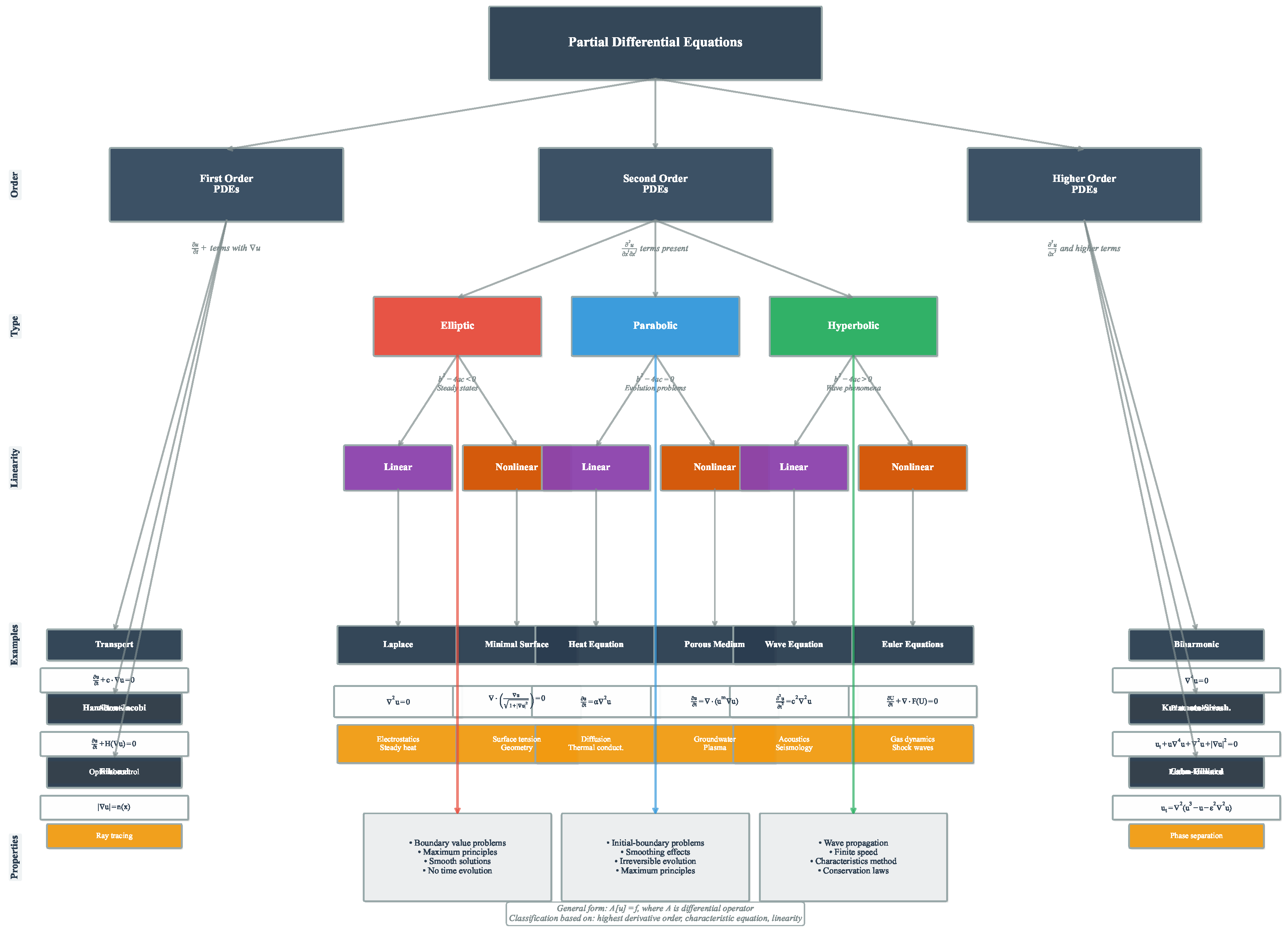
Figure 2.
Mathematical framework illustrating the progression from physical phenomena to PDE analysis. The diagram shows the systematic flow from physical modeling through PDE formulation to theoretical analysis, emphasizing the hierarchical nature of solution concepts. The central pathway demonstrates the generalization from classical solutions (requiring twice differentiability and point-wise satisfaction) through weak solutions (integral formulations with data) to distributional solutions (test function formulations accommodating singular solutions). The regularity ladder displays the progression of function spaces from continuous () to smooth () functions, including Sobolev spaces (, ) that bridge classical and weak formulations. Key embedding theorems (Sobolev, Hölder, Rellich, Gagliardo-Nirenberg) establish critical relationships between function spaces. Well-posedness criteria (existence, uniqueness, stability) and variational formulation procedures provide the theoretical foundation ensuring mathematically sound problem formulation and analysis.
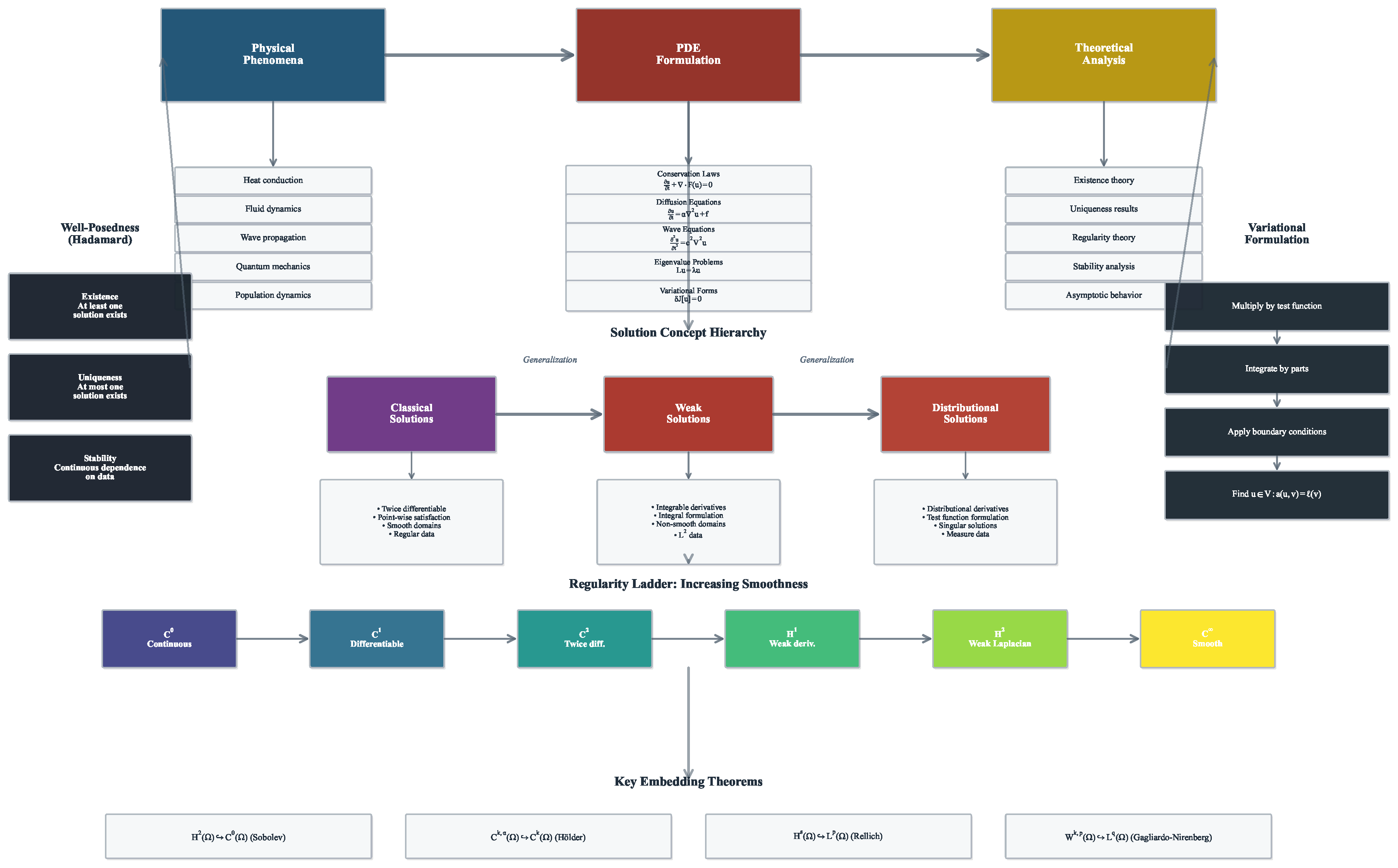
Figure 3.
Overview of the five major computational challenges in PDE analysis. Challenge 1 illustrates the curse of dimensionality, showing exponential growth in computational complexity from N to as dimensions increase, with applications ranging from financial option pricing ( grid points) to quantum many-body systems. Challenge 2 depicts the transition from predictable linear behavior to chaotic nonlinear dynamics, highlighting phenomena such as turbulence, solitons, and bifurcations where small changes produce large effects. Challenge 3 demonstrates geometric complexity progression from simple rectangular domains to extreme multi-scale geometries encountered in aerospace, biomedical, and materials applications. Challenge 4 visualizes discontinuity types including shock waves, material interfaces, and free boundaries, along with associated numerical difficulties such as Gibbs oscillations and spurious reflections. Challenge 5 presents the multiscale hierarchy from molecular ( m) to global ( m) scales, emphasizing the computational burden of direct resolution requiring degrees of freedom and the need for specialized approaches such as homogenization and model reduction techniques.
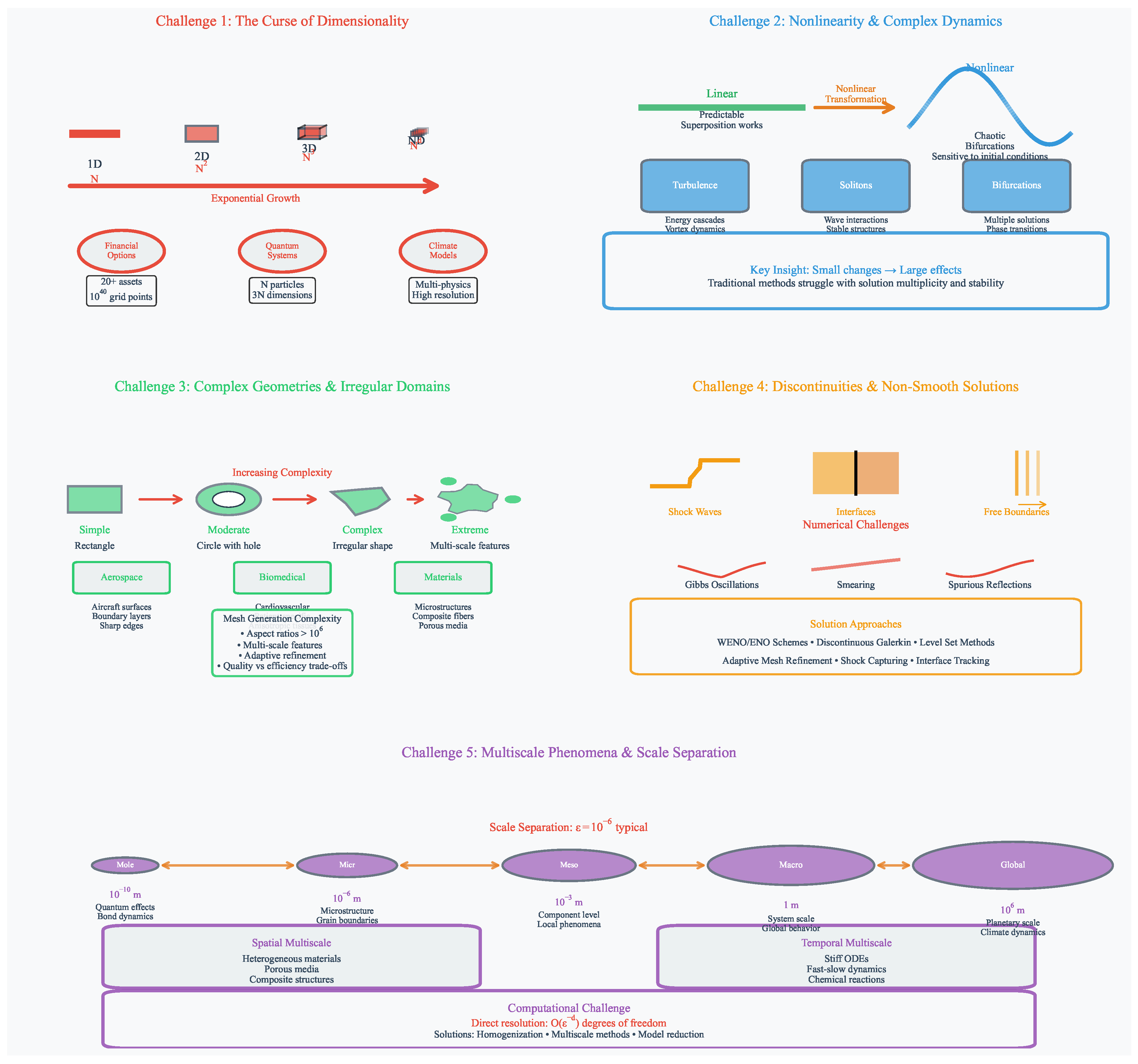
Figure 4.
Historical evolution of PDE solution methods from the 1700s to the 2020s, presented as an integrated timeline. The main flowing timeline traces four major eras: Analytical Foundations (1697-1900) with developments from Leibniz’s first variational methods through Fourier analysis and Green’s functions; Early Numerical Methods (1900-1960) encompassing the Ritz and Galerkin formulations, CFL stability conditions, and Courant’s pioneering finite elements; Modern Computational Era (1960-2010) featuring industrial software development (NASTRAN), spectral methods, multigrid algorithms, and adaptive techniques; and Machine Learning Integration (2010-2025) introducing physics-informed neural networks, neural operators, and hybrid physics-ML approaches. Method evolution trees extend from the main timeline showing the development of analytical methods, finite differences, finite elements, spectral methods, and neural approaches with their respective branches. The computational scale evolution panel displays the progression from hand calculations to parameter models. Century markers at the bottom provide temporal anchoring with visual connections to corresponding timeline positions, while breakthrough achievements are highlighted with distinctive markers. The visualization captures over 3 centuries of method development, demonstrating the acceleration from theoretical foundations through computational revolution to contemporary machine learning integration.
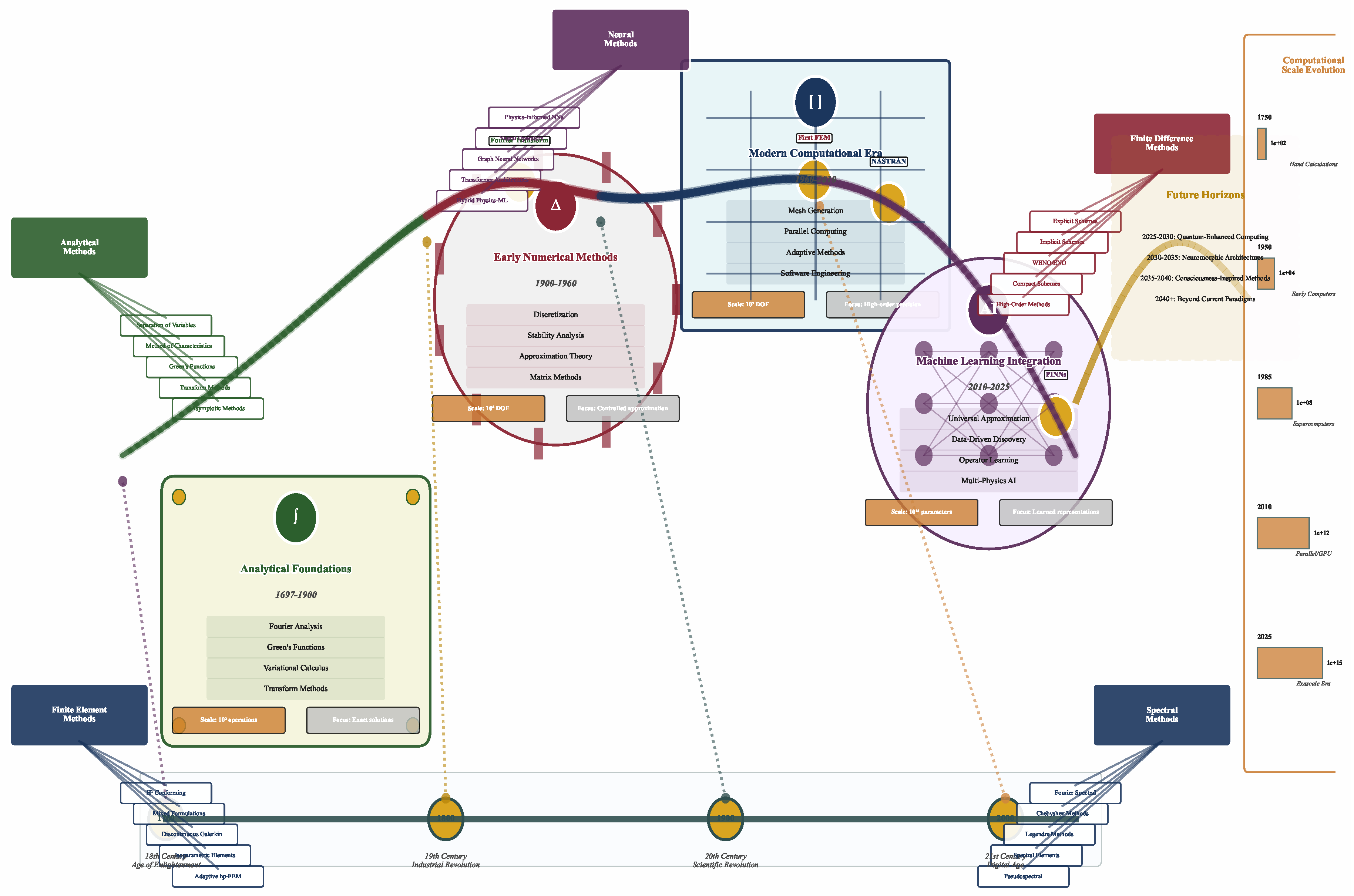
Figure 5.
Historical evolution of machine learning methods (1943-2025). The timeline displays major milestones across four technological epochs: Theoretical Foundations (1943-1970, blue) establishing mathematical frameworks including the McCulloch-Pitts neuron model, perceptron learning, and automatic differentiation; Methodological Development (1971-2011, teal) introducing practical algorithms such as backpropagation, universal approximation theory, and LSTM networks; Deep Learning Renaissance (2012-2016, green) marked by computational breakthroughs including AlexNet, generative adversarial networks, and optimization advances; and Scientific Machine Learning Era (2017-present, red) featuring physics-informed approaches like PINNs, neural operators, and foundation models.
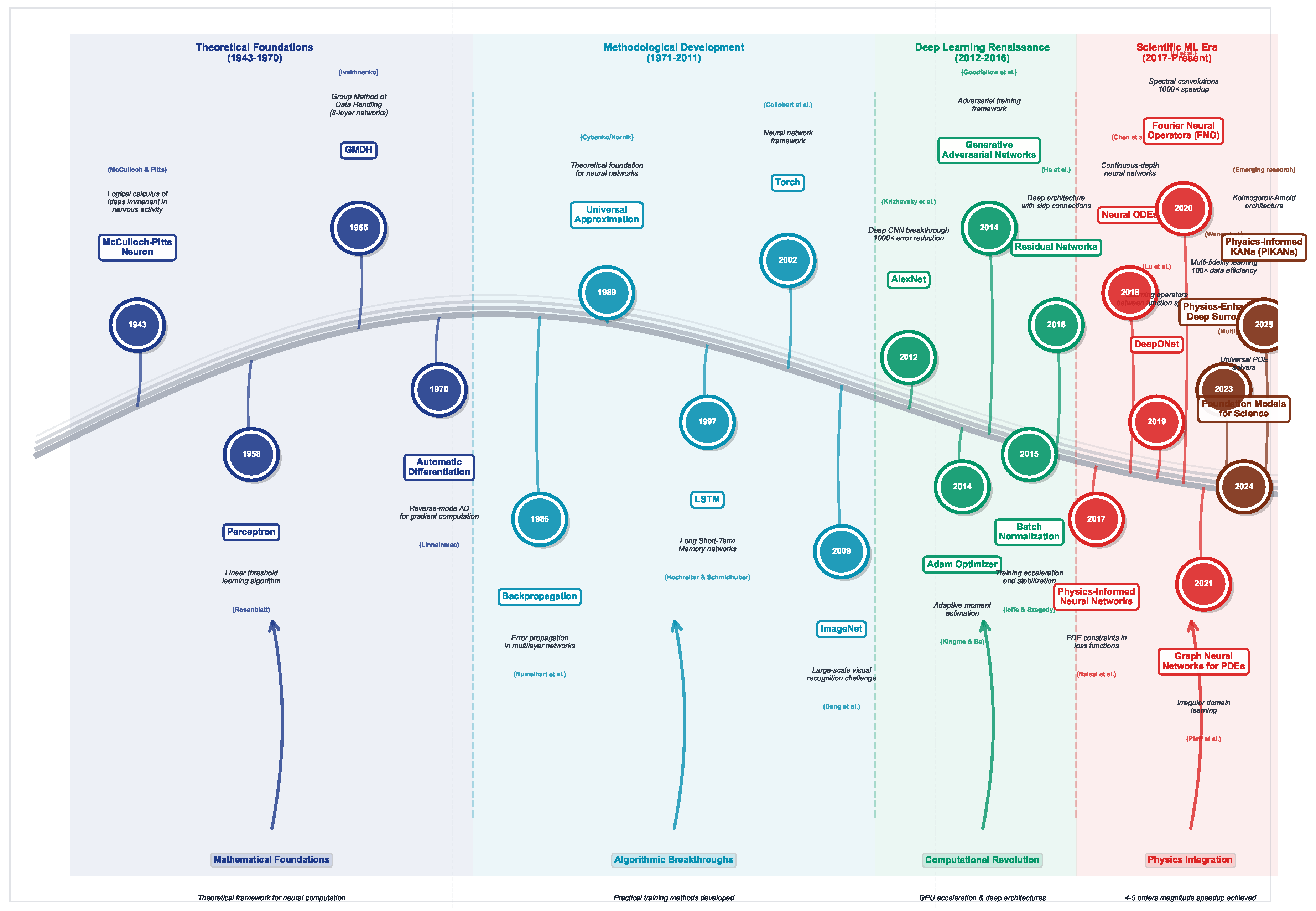
Figure 6.
Comparison matrix of traditional PDE solving methods. The central table provides detailed analysis across nine critical dimensions: discretization approach, accuracy order, geometric flexibility, conservation properties, implementation complexity, computational scaling, memory patterns, and primary applications. Performance ratings use a five-tier scale from excellent to poor, with color coding for visual clarity. Conservation properties distinguish between methods providing exact local conservation (finite volume), global conservation only (finite element), or both local and global conservation (discontinuous Galerkin). Accuracy orders range from for basic finite volume schemes to exponential convergence for spectral methods on smooth solutions. Computational scaling varies from optimal linear scaling for finite differences to cubic scaling for boundary element methods. Four radar charts highlight the performance profiles of key methods across accuracy, geometric flexibility, computational efficiency, and implementation simplicity. The method selection guide provides application-specific recommendations based on problem characteristics such as geometry complexity, conservation requirements, and accuracy demands. Performance indicator bars adjacent to method names provide rapid visual assessment of relative strengths across four key performance indicators (accuracy, flexibility, efficiency, and implementation).
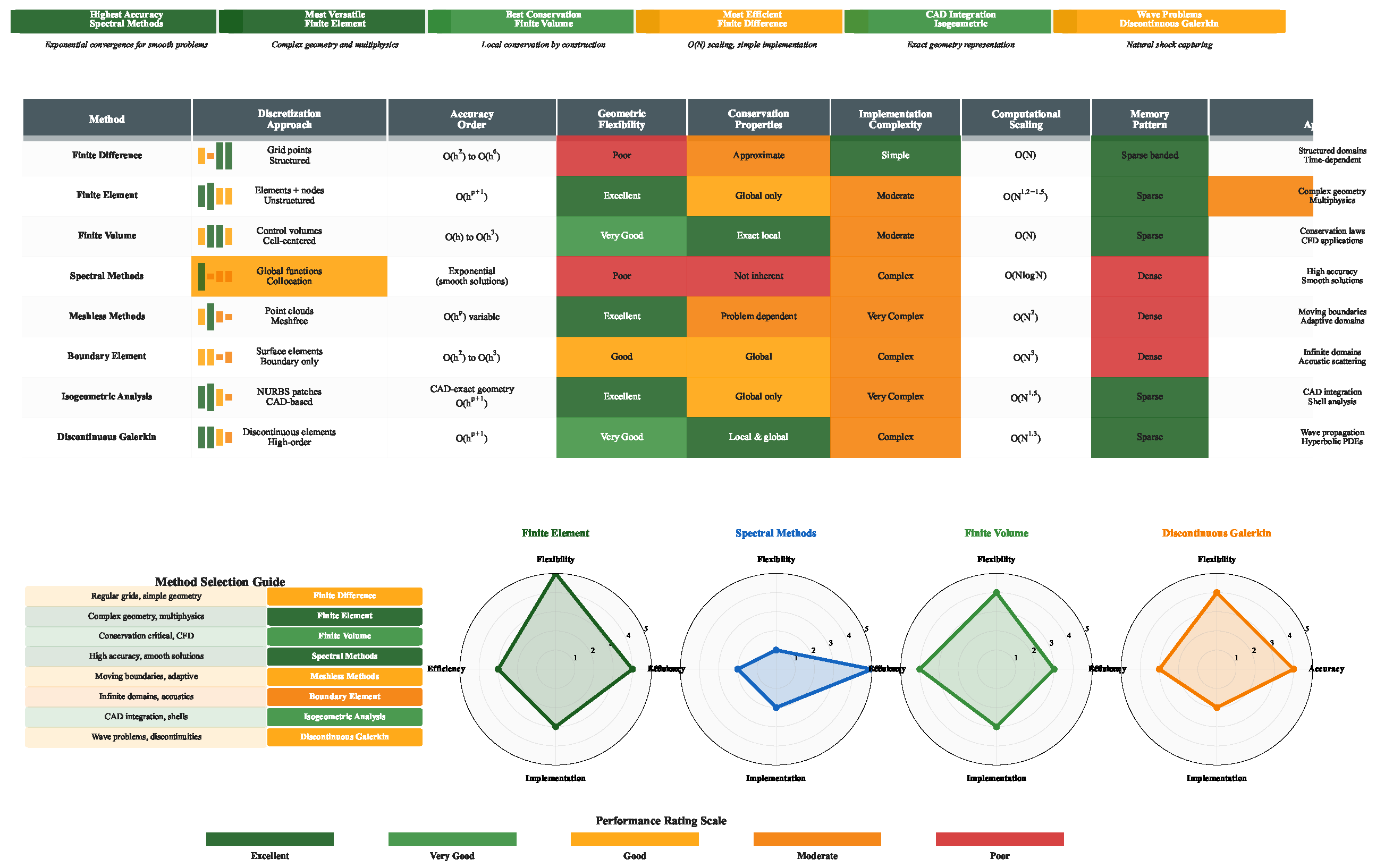
Figure 7.
Machine learning method families for solving PDEs. This visualization presents a systematic overview of major ML-based approaches for PDE solutions, organized by their development timeline (2016-2025) and performance characteristics. Each method card displays: (i) core algorithmic principle and year of introduction, (ii) quantitative performance metrics across four dimensions (accuracy, computational speed, flexibility, and maturity), (iii) computational complexity scaling, (iv) data requirements, and (v) primary application domains. The ecosystem includes established methods such as Physics-Informed Neural Networks (PINNs) for minimal-data scenarios, Neural Operators (FNO/DeepONet) for parametric studies, and Graph Neural Networks (GNNs) for irregular geometries, alongside emerging approaches like Physics-Enhanced Deep Surrogates (PEDS) and the DeePoly framework.

Figure 8.
Evolutionary genealogy of machine learning methods for differential equations. The network diagram displays methodological inheritance patterns across four technological epochs, with nodes representing individual innovations positioned chronologically along the horizontal axis. Node colors distinguish methodological categories: foundations (blue) establishing mathematical frameworks, classical machine learning (cyan) developing practical algorithms, deep learning renaissance (emerald) introducing computational breakthroughs, scientific machine learning (red) integrating physics constraints, neural operators (orange-red) achieving spectral methods, physics-informed approaches (amber) embedding differential equations, hybrid methods (indigo) combining multiple paradigms, and recent advances (purple) representing current developments. Directed arrows show influence relationships, with line thickness and opacity encoding influence strength based on temporal proximity and methodological significance. Solid arrows represent direct algorithmic inheritance, while dashed lines indicate conceptual influences across longer periods. Star markers identify paradigm-shifting breakthroughs that fundamentally altered subsequent research trajectories.
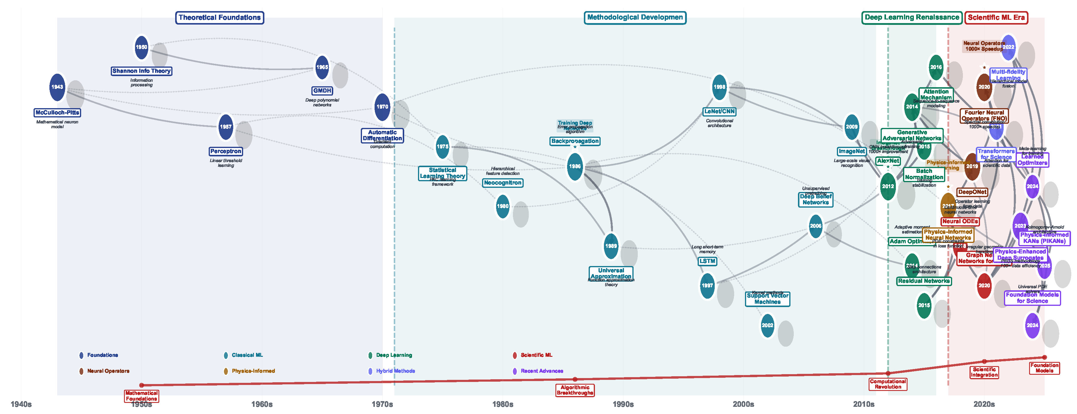
Figure 9.
Synthesis framework for PDE solver development through the next decade. (a) Challenge landscape assessment with bubble sizes indicating timeline complexity and colors representing breakthrough probability, where eight major challenge domains are positioned according to research difficulty and potential impact. (b) Technology synthesis architecture showing integration flows between traditional methods, foundation models, hybrid approaches, quantum computing, verification frameworks, uncertainty quantification systems, real-time deployment capabilities, and multi-domain applications. (c) Technology readiness evolution from the current 2025 status through projected 2030 and 2035 capabilities, subjected to confidence intervals due to complexity, R&D intensity, and funding availability. (d) Theoretical foundation landscapes across six key domains, comparing current understanding levels with research activity intensity and breakthrough potential to identify critical knowledge gaps. (e) Performance trajectory evolution on a logarithmic scale for traditional, neural, hybrid, and quantum methods from 2020 to 2035, with vertical markers indicating breakthrough milestones including foundation model emergence and potential quantum advantage. (f) Synthesis success metrics tracking progress across accuracy improvement, computational speed enhancement, implementation complexity reduction, industrial adoption rates, scientific credibility establishment, and educational integration, with horizontal threshold lines marking acceptable, good, and excellent performance levels.
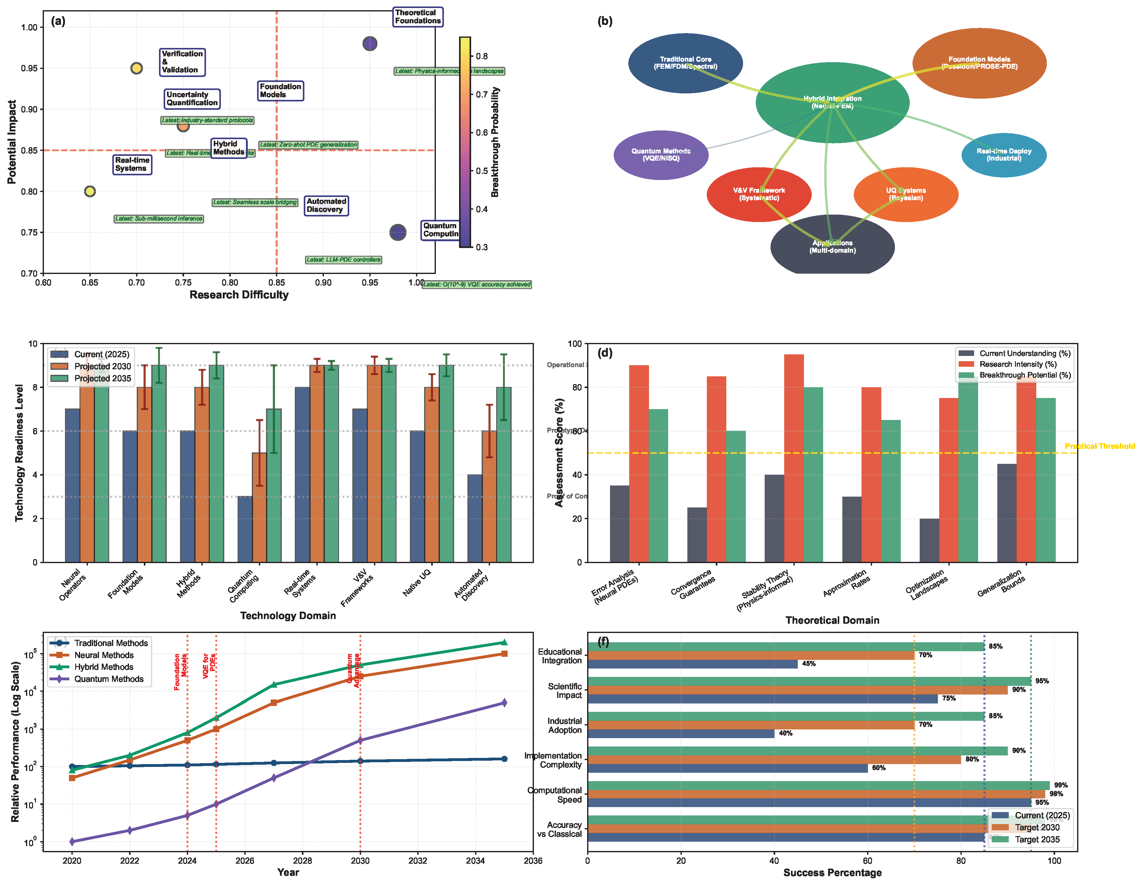

Table 1.
Comparison of classical and multiscale PDE solvers with respect to computational complexity, adaptivity, uncertainty quantification capabilities, and implementation characteristics. This table provides a detailed overview of established mathematical methods for solving PDEs, including their computational scaling behavior, mesh adaptivity features, support for uncertainty quantification (UQ), nonlinearity handling approaches, theoretical error guarantees, implementation complexity, typical error ranges, and key implementation notes.
| Method | Complexity | Mesh | UQ | Nonlinearity | Theory | Impl. | Error | Implementation Notes |
| Adapt. | Handling | Bounds | Diff. | |||||
| Classical Finite Difference Methods | ||||||||
| Finite Difference (FDM) | to | None | No | Explicit/Implicit | Partial | Low | to | Simple stencil operations; CFL stability conditions for explicit schemes |
| Compact FD Schemes | None | No | Implicit | Strong | Medium | to | Higher-order accuracy; tridiagonal systems; Padé approximations | |
| Weighted Essentially Non-Osc. | None | No | Conservative | Strong | High | to | High-order shock capturing; nonlinear weights; TVD property | |
| Classical Finite Element Methods | ||||||||
| Standard FEM (h-version) | to | h-refine | Limited | Newton-Raphson | Strong | Medium | to | Variational formulation; sparse matrix assembly; a priori error estimates |
| p-Finite Element | to | p-refine | Limited | Newton-Raphson | Strong | High | to | High-order polynomials; hierarchical basis; exponential convergence |
| hp-Finite Element | to | hp-adapt | Limited | Newton-Raphson | Strong | Very High | to | Optimal convergence rates; automatic hp-adaptivity algorithms |
| Mixed Finite Element | to | h-adapt | No | Saddle point | Strong | High | to | inf-sup stability; Brezzi conditions; simultaneous approximation |
| Discontinuous Galerkin | to | hp-adapt | No | Explicit/Implicit | Strong | High | to | Local conservation; numerical fluxes; upwinding for hyperbolic PDEs |
| Spectral and High-Order Methods | ||||||||
| Global Spectral Method | None | No | Pseudo-spectral | Strong | Medium | to | FFT-based transforms; exponential accuracy for smooth solutions | |
| Spectral Element Method | p-adapt | No | Newton-Raphson | Strong | High | to | Gauss-Lobatto-Legendre points; tensorized basis functions | |
| Chebyshev Spectral | None | No | Collocation | Strong | Medium | to | Chebyshev polynomials; Clenshaw-Curtis quadrature | |
| Finite Volume and Conservative Methods | ||||||||
| Finite Volume Method | to | r-adapt | No | Godunov/MUSCL | Partial | Medium | to | Conservation laws; Riemann solvers; flux limiters for monotonicity |
| Cell-Centered FV | AMR | No | Conservative | Partial | Medium | to | Dual mesh approach; reconstruction procedures; slope limiters | |
| Vertex-Centered FV | Unstructured | No | Conservative | Partial | High | to | Median dual cells; edge-based data structures | |
| Advanced Grid-Based Methods | ||||||||
| Adaptive Mesh Refinement | to | Dynamic | No | Explicit/Implicit | Partial | High | to | Hierarchical grid structures; error estimation; load balancing |
| Multigrid Method | Limited | No | V/W-cycles | Strong | High | to | Prolongation/restriction operators; coarse grid correction | |
| Algebraic Multigrid | Graph-based | No | Nonlinear | Strong | Very High | to | Strength of connection; coarsening algorithms; smoothing | |
| Block-Structured AMR | Structured | No | Conservative | Partial | Very High | to | Berger-Colella framework; refluxing; subcycling in time | |
| Meshless Methods | ||||||||
| Method of Fundamental Sol. | None | No | Direct solve | Strong | Medium | to | Fundamental solutions; boundary collocation; no mesh required | |
| Radial Basis Functions | None | No | Global interp. | Weak | High | to | Shape parameter selection; ill-conditioning issues | |
| Meshless Local Petrov-Gal. | Nodal | No | Moving LS | Partial | High | to | Local weak forms; weight functions; integration difficulties | |
| Smooth Particle Hydrodynamics | Lagrangian | No | Explicit | Weak | Medium | to | Kernel approximation; artificial viscosity; particle inconsistency | |
| Specialized Classical Methods | ||||||||
| Boundary Element Method | to | Surface | No | Integral eq. | Strong | High | to | Green’s functions; singular integrals; infinite domains |
| Fast Multipole BEM | Surface | No | Hierarchical | Strong | Very High | to | Tree algorithms; multipole expansions; translation operators | |
| Isogeometric Analysis | k-refinement | No | Newton-Raphson | Strong | High | to | NURBS basis functions; exact geometry; higher continuity | |
| eXtended FEM (XFEM) | Enrichment | No | Level sets | Partial | Very High | to | Partition of unity; discontinuities without remeshing | |
| Multiscale Methods | ||||||||
| Multiscale FEM (MsFEM) | Coarse | No | Implicit | Strong | High | to | Offline basis construction; scale separation; periodic microstructure | |
| Generalized MsFEM | Coarse | No | Implicit | Strong | Very High | to | Spectral basis functions; local eigenvalue problems; oversampling | |
| Heterogeneous Multiscale | Macro | Limited | Constrained | Strong | Very High | to | Macro-micro coupling; constrained problems; missing data | |
| Localized Orthogonal Dec. | Local | No | Implicit | Strong | Very High | to | Exponential decay; corrector problems; quasi-local operators | |
| Variational Multiscale | Coarse | No | Stabilized | Strong | High | to | Fine-scale modeling; residual-based stabilization; bubble functions | |
| Equation-Free Methods | Microscopic | No | Projective | Emerging | Very High | to | Coarse projective integration; gap-tooth schemes; patch dynamics | |
| Two-Scale FEM | Hierarchical | No | Computational | Strong | Very High | to | Representative volume elements; computational homogenization | |
| Reduced Basis Method | Parameter | Yes | Affine decomp. | Strong | High | to | Greedy selection; a posteriori error bounds; parametric problems | |
Legend: N = degrees of freedom, = coarse grid size, = fine grid size, = macro scale, = micro scale, = reduced basis dimension, k = number of basis functions, d = spatial dimension. Theory Bounds: Strong = rigorous a priori/posteriori estimates, Partial = limited theoretical results, Weak = heuristic bounds, Emerging = active research area. Implementation Difficulty: Low = basic programming, Medium = moderate expertise, High = advanced knowledge, Very High = specialized expertise required. UQ Support: Limited = can incorporate basic uncertainty through Monte Carlo, Yes = native uncertainty quantification capabilities.
Table 2.
Overview of outlined ML-based PDE Solver families in the section below.
| Method Family | Key Principle | Typical Applications | Computational Scaling | Data Requirements |
|---|---|---|---|---|
| Physics-Informed NNs | Embed PDE in loss function | General PDEs, inverse problems | Minimal | |
| Neural Operators | Learn function-to-function mappings | Parametric PDEs, multi-query | Moderate to High | |
| Graph Neural Networks | Message passing on meshes | Irregular geometries, adaptive | Moderate | |
| Transformer-Based | Attention mechanisms | Long-range dependencies | to | High |
| Generative Models | Probabilistic solutions | Uncertainty quantification | Problem-dependent | Moderate |
| Hybrid Methods | Combine ML with traditional | Multi-physics, multi-scale | Varies | Moderate |
| Meta-Learning | Rapid adaptation | Few-shot problems, families | Low per task | |
| Physics Enhanced Deep Surrogates | Low-fidelity + neural correction | Complex physical systems | ∼10× less | |
| Random Feature Methods | Random feature functions | Bridge traditional/ML | Low to Moderate | |
| DeePoly Framework | Two-stage DNN+polynomial | High-order accuracy | Moderate | |
| Specialized Architectures | Domain-specific designs | Specific PDE classes | Architecture-dependent | Varies |
Table 3.
Comparison of modern machine learning-based PDE solvers: Architecture types, computational complexity, multiscale capabilities, and implementation characteristics. This table provides a detailed analysis of state-of-the-art neural methods for solving PDEs, including their architectural foundations, training complexity, inference speed, multiscale handling, nonlinearity treatment, uncertainty quantification (UQ) capabilities, typical accuracy ranges, and key implementation notes.
| Method | Architecture Type | Training Complex. | UQ | Multiscale Capability | Nonlinearity Handling | Inference Speed | Accuracy Range | Implementation Notes & Key Features |
| Physics-Informed Neural Networks (PINNs) Family | ||||||||
| Physics-Informed NNs | Residual-based | Limited | Moderate | Sensitive | Fast | to | Automatic differentiation for PDE residuals; weak BC enforcement; spectral bias issues | |
| Variational PINNs | Weak formulation | Moderate | Improved | Better | Fast | to | Galerkin projection; better conditioning than PINNs; requires integration | |
| Conservative PINNs | Energy-preserving | No | Moderate | Physical | Fast | to | Hamiltonian structure preservation; symplectic integration principles | |
| Deep Ritz Method | Variational approach | No | Limited | Smooth | Fast | to | Energy minimization; requires known energy functional; high-dimensional problems | |
| Weak Adversarial Networks | Min-max formulation | No | Moderate | Good | Medium | to | Adversarial training; dual formulation; improved boundary handling | |
| Extended PINNs (XPINNs) | Domain decomposition | No | Good | Moderate | Medium | to | Subdomain coupling; interface conditions; parallel training capability | |
| Multi-fidelity PINNs | Hierarchical data | Yes | Good | Moderate | Fast | to | Multiple data fidelities; transfer learning; uncertainty propagation | |
| Adaptive PINNs | Residual-based adapt. | Limited | Good | Moderate | Medium | to | Residual-based point refinement; gradient-enhanced sampling | |
| Neural Operator Methods | ||||||||
| Fourier Neural Operator | Fourier transform | Ensemble | Limited | Periodic | Very Fast | to | FFT-based convolutions; resolution invariance; periodic boundary assumption | |
| DeepONet | Branch-trunk arch. | Dropout | Moderate | Smooth | Fast | to | Universal operator approximation; separable architecture; sensor placement critical | |
| Graph Neural Operator | Graph convolution | Limited | Good | Moderate | Fast | to | Irregular geometries; message passing; edge feature learning | |
| Multipole Graph Networks | Hierarchical graphs | No | Very Good | Good | Fast | to | Fast multipole method inspiration; multiscale graph pooling | |
| Neural Integral Operator | Integral kernels | Limited | Moderate | Good | Medium | to | Learned Green’s functions; non-local operators; memory intensive | |
| Wavelet Neural Operator | Wavelet basis | No | Very Good | Good | Fast | to | Multiscale wavelet decomposition; adaptive resolution; boundary wavelets | |
| Transformer Neural Op. | Self-attention | Attention | Good | Good | Medium | to | Global receptive field; positional encoding for coordinates | |
| LSM-based Neural Op. | Least squares | Variance | Moderate | Linear | Fast | to | Moving least squares kernels; local approximation; meshfree approach | |
| Graph Neural Network Approaches | ||||||||
| MeshGraphNets | Message passing | Limited | Good | Good | Fast | to | Mesh-based GNNs; temporal evolution; learned physics dynamics | |
| Neural Mesh Refinement | Adaptive graphs | No | Very Good | Moderate | Medium | to | Dynamic mesh adaptation; error-driven refinement; graph coarsening | |
| Multiscale GNNs | Hierarchical pooling | Limited | Very Good | Good | Fast | to | Graph U-Net architecture; multiscale feature extraction | |
| Physics-Informed GNNs | Residual constraints | No | Good | Good | Fast | to | PDE residuals as graph losses; physics-constrained message passing | |
| Geometric Deep Learning | Equivariant layers | Limited | Moderate | Good | Fast | to | SE(3) equivariance; geometric priors; irreducible representations | |
| Simplicial Neural Nets | Simplicial complexes | No | Good | Moderate | Medium | to | Higher-order interactions; topological features; persistent homology | |
| Transformer and Attention-Based Methods | ||||||||
| Galerkin Transformer | Spectral attention | Limited | Good | Good | Medium | to | Fourier attention mechanism; spectral bias mitigation | |
| Factorized FNO | Low-rank approx. | No | Moderate | Good | Fast | to | Tucker decomposition; reduced complexity; maintains accuracy | |
| U-FNO | U-Net + FNO | Limited | Very Good | Good | Fast | to | Encoder-decoder structure; multiscale processing; skip connections | |
| Operator Transformer | Cross-attention | Attention | Good | Good | Medium | to | Input-output cross-attention; flexible geometries | |
| PDEformer | Autoregressive | Limited | Moderate | Sequential | Medium | to | Time-stepping transformer; causal attention masks | |
| Generative and Probabilistic Models | ||||||||
| Score-based PDE Solvers | Diffusion models | Native | Limited | Stochastic | Slow | to | Denoising score matching; probabilistic solutions; sampling-based inference | |
| Variational Autoencoders | Latent space | Native | Good | Moderate | Fast | to | Dimensionality reduction; probabilistic encoding; KL regularization | |
| Normalizing Flows | Invertible transforms | Native | Limited | Good | Medium | to | Exact likelihood computation; invertible neural networks | |
| Neural Stochastic PDEs | Stochastic processes | Native | Good | Stochastic | Medium | to | SDE neural networks; path sampling; Wiener process modeling | |
| Bayesian Neural Nets | Posterior sampling | Native | Moderate | Good | Slow | to | Weight uncertainty; Monte Carlo dropout; variational inference | |
| Hybrid and Multi-Physics Methods | ||||||||
| Neural-FEM Coupling | Hybrid discretization | Limited | Very Good | Good | Medium | to | FEM backbone with neural corrections; domain decomposition | |
| Multiscale Neural Nets | Scale separation | Limited | Very Good | Good | Fast | to | Explicit scale separation; homogenization-inspired; scale bridging | |
| Neural Homogenization | Effective properties | Limited | Very Good | Moderate | Fast | to | Representative volume elements; effective medium theory | |
| Multi-fidelity Networks | Data fusion | Good | Good | Moderate | Fast | to | Information fusion; transfer learning; cost-accuracy tradeoffs | |
| Physics-Guided Networks | Domain knowledge | Limited | Good | Physics | Fast | to | Hard constraints; conservation laws; invariance properties | |
| Specialized Architectures | ||||||||
| Convolutional Neural Op. | CNN-based | Limited | Limited | Good | Very Fast | to | Translation equivariance; local receptive fields; parameter sharing | |
| Recurrent Neural PDE | Sequential processing | Limited | Moderate | Temporal | Medium | to | Time-dependent PDEs; memory mechanisms; gradient issues | |
| Capsule Networks | Hierarchical features | No | Good | Moderate | Medium | to | Part-whole relationships; routing algorithms; viewpoint invariance | |
| Neural ODEs for PDEs | Continuous dynamics | Limited | Good | Continuous | Slow | to | Continuous-time modeling; adaptive stepping; memory efficient | |
| Quantum Neural Networks | Quantum computing | Quantum | Limited | Quantum | Slow | to | Quantum advantage potential; NISQ limitations; exponential speedup theory | |
| Meta-Learning and Few-Shot Methods | ||||||||
| MAML for PDEs | Gradient-based | Limited | Moderate | Transfer | Fast | to | Model-agnostic meta-learning; few-shot adaptation; gradient-based | |
| Prototypical Networks | Prototype matching | Limited | Limited | Metric | Fast | to | Metric learning; prototype computation; episodic training | |
| Neural Process for PDEs | Stochastic processes | Native | Good | Contextual | Fast | to | Context-target paradigm; uncertainty quantification; function-space priors | |
| Hypernetworks | Parameter generation | Limited | Good | Adaptive | Fast | to | Weight generation; task conditioning; parameter sharing | |
| Legend:N = problem size, E = graph edges, T = time steps, L = layers, d = dimension, k = polynomial degree, r = rank, h = hidden size, P = parameters. | ||||||||
| Training Complexity: Typical computational cost for training phase; varies significantly with problem size and architecture. | ||||||||
| UQ Capability: Native = built-in uncertainty quantification, Ensemble = multiple model averaging, Limited = requires extensions. | ||||||||
| Inference Speed: Very Fast = ms, Fast = ms, Medium = 100ms-1s, Slow = s for typical problems. | ||||||||
| Accuracy Range: Typical relative error on standard benchmarks; highly problem-dependent. | ||||||||
Disclaimer/Publisher’s Note: The statements, opinions and data contained in all publications are solely those of the individual author(s) and contributor(s) and not of MDPI and/or the editor(s). MDPI and/or the editor(s) disclaim responsibility for any injury to people or property resulting from any ideas, methods, instructions or products referred to in the content. |
© 2025 by the authors. Licensee MDPI, Basel, Switzerland. This article is an open access article distributed under the terms and conditions of the Creative Commons Attribution (CC BY) license (http://creativecommons.org/licenses/by/4.0/).
Copyright: This open access article is published under a Creative Commons CC BY 4.0 license, which permit the free download, distribution, and reuse, provided that the author and preprint are cited in any reuse.


