

Submitted:
21 June 2026
Posted:
22 June 2026
You are already at the latest version
Abstract
Electrochemically induced stress and strain energy are key factors governing mechanical degradation in battery electrodes during repeated ion insertion and extraction. However, their quantitative evaluation remains challenging. In this work, we present theoretical frameworks for describing the evolution of stress, strain energy, and elastic modulus in battery electrodes during electrochemical cycling. First, we discuss the general concepts of chemical strain, stress, and strain energy developed in substrate-bonded thin-film electrodes during ion insertion under the assumptions of elasticity and small deformation. Second, we present a general framework for estimating the apparent Young’s modulus of porous composite electrodes, which also enables inverse identification of the Young’s modulus of active materials when the apparent Young’s modulus of the porous composite electrode is experimentally available. Then, frameworks for estimating mechanical work and elastic strain energy of a substrate-constrained electrode during ion insertion with concentration-dependent thickness and modulus are discussed. Finally, we present inverse chemo-mechanical frameworks for diffusion-induced stress and concentration-dependent modulus in substrate-constrained electrodes under single-step galvanostatic ion insertion/extraction and galvanostatic insertion–extraction cycling. When combined with experimental measurements, these frameworks provide quantitative methods for understanding the evolution of stress, modulus, and strain energy in practical battery electrodes and offer guidance for the mechanical design of high-performance electrode materials.
Keywords:
stress
; strain energy
; chemical strain
; composite electrode
; ion insertion
; modulus
Introduction
Stress and strain energy evolution during battery cycling critically governs electrode degradation and performance decline [1,2]. During electrochemical cycling, ion concentration variations induce dimensional/volume changes in electrodes. These changes generate two distinct stress contributions: (1) diffusion-induced stresses (DIS) arising from concentration gradients within active particles [3,4], and (2) macroscopic electrode level stresses in film-substrate electrode systems caused by constraints from inactive cell components (e.g., current collectors) and geometric limitations [2,5,6,7,8,9]. These stresses trigger mechanical degradation through electrode fracturing, particle disintegration, and contact loss at interfaces, ultimately causing capacity fade and cell failure [6,10,11,12,13]. Meanwhile, the strain energy accumulated during deformation drives crack initiation and propagation as stored energy converts to surface energy during fracture [14]. Notably, cracks could originate at active/inactive material interfaces and within the active particles, emphasizing the necessity to study DIS and strain energy evolution at both electrode and particle levels.
Real-time observation techniques, such as in situ X-ray or electron-based microscopy, reveal atomic-scale deformation mechanisms but lack direct stress/strain quantification in practical porous composite electrodes composed of active particles, binders, and conductive agents [15,16,17]. Such investigations were made possible by the use of digital image correlation (DIC) or laser-based techniques employing Stoney’s equation combined with chemo-mechanical modeling [9,18,19,20,21]. Although theoretical studies have addressed DIS and strain energy at particle scales [14,22,23,24,25], electrode-level investigations remain limited. Bridging this gap is essential to mitigate fracture-related degradation and optimize next-generation batteries through stress-engineered electrode designs.
This work presents a systematic theoretical treatment of the evolution of stress, strain energy, and modulus in practical thin-film composite battery electrodes coated on current collectors during ion insertion and extraction. The proposed frameworks are based on small-deformation elasticity. Section I introduces the general concepts of chemical strain, stress, and strain energy developed in substrate-bonded thin-film electrodes during ion insertion under elastic, small-deformation assumptions. Section II presents a general framework for estimating the apparent Young’s modulus of porous composite electrodes, which also enables inverse identification of the Young’s modulus of active materials when the apparent Young’s modulus of the porous composite electrode is available experimentally. Section III discusses frameworks for estimating the mechanical work and elastic strain energy of a substrate-constrained electrode during ion insertion when both thickness and modulus depend on concentration. Section IV presents a general framework for estimating stress in an active electrode film–current collector bilayer from curvature evolution under the assumption of spatially uniform concentration. Sections V and VI present inverse chemo-mechanical frameworks for determining diffusion-induced stress and concentration-dependent modulus in substrate-constrained electrodes under single-step galvanostatic ion insertion/extraction and galvanostatic insertion–extraction cycling conditions, respectively.
I. General Concepts of Chemical Strain, Stress, and Strain Energy Developed in a Substrate-Bonded Thin Film Electrode During Lithium Insertion Under Linear Elasticity
The theoretical frameworks presented in this work aim to evaluate stress, modulus, and strain energy variation during electrochemical ion insertion and extraction in practical composite battery electrodes bonded to current collector substrates. The practical electrode is generally a porous heterogeneous composite consisting of active materials, conductive additives, binders, and pores. In the present work, the electrode is assumed to be isotropic with respect to its compositional, structural, and mechanical properties, although it may contain anisotropic active particles.
Ion diffusion within the electrode generally gives rise to concentration gradients, the extent of which depends on the magnitude of the ion flux or current densities. In certain limiting cases, a spatially homogeneous ion concentration is assumed within the electrode. This assumption is justified for sufficiently thin electrodes, low current densities, or situations in which solid-state diffusion occurs on time scales much shorter than that of electrochemical cycling. Under these conditions, electrode-scale concentration gradients are negligible, and the electrochemically induced expansion/contraction can be represented by an average concentration-dependent chemical strain.
Because the electrode is bonded to a substrate, free in-plane expansion or contraction of the film is suppressed during ion insertion and extraction. As a result, concentration changes generate a mismatch between the natural chemical swelling strain of the electrode and the actual kinematically admissible deformation, which gives rise to in-plane stress. The top surface of the film is traction-free, so that the out-of-plane normal stress is negligible compared with the in-plane stress. Under these assumptions, the electrode develops an equi-biaxial in-plane stress state,
Because ion insertion induces a stress-free chemical strain of the electrode, the total strain is decomposed into a mechanical strain and a chemical strain as
(1-1)
where , , and denote the total strain, mechanical strain, and chemical strain of the electrode, respectively. The superscript e indicates electrode. Since the chemical strain only occurs in electrode, the superscript e is omitted in .
Only the mechanical strain contributes to stress generation. Under the assumptions of plane stress, small deformation, and linear elasticity, the in-plane stress components are expressed as
(1-2a)
(1-2b)
where and are the apparent or effective Young’s modulus and Poisson’s ratio of the composite electrode, respectively. The superscript e is also omitted since the apparent or effective mechanical properties are only applicable for the composite electrode. , , and denote the total strain and chemical strain of the active electrode film along the xx and yy directions, respectively. These quantities correspond to normal strain components. For simplicity, the subscripts xx and yy are replaced by x and y, respectively.
The corresponding shear stress is given by
, (1-3)
where
(1-4)
is the apparent or effective shear modulus of the composite electrode, and is the mechanical shear strain. For isotropic chemical expansion, . If the in-plane deformation is equi-biaxial and shear deformation is negligible, i.e., and , the in-plane stresses reduce to
(1-5)
This expression shows that stress is generated only when the electrochemically induced chemical expansion is mechanically constrained. For a freestanding electrode, ion insertion produces a stress-free chemical expansion, and the total strain equals the chemical strain, i.e., . Therefore, no macroscopic in-plane stress is generated in the absence of external constraints.
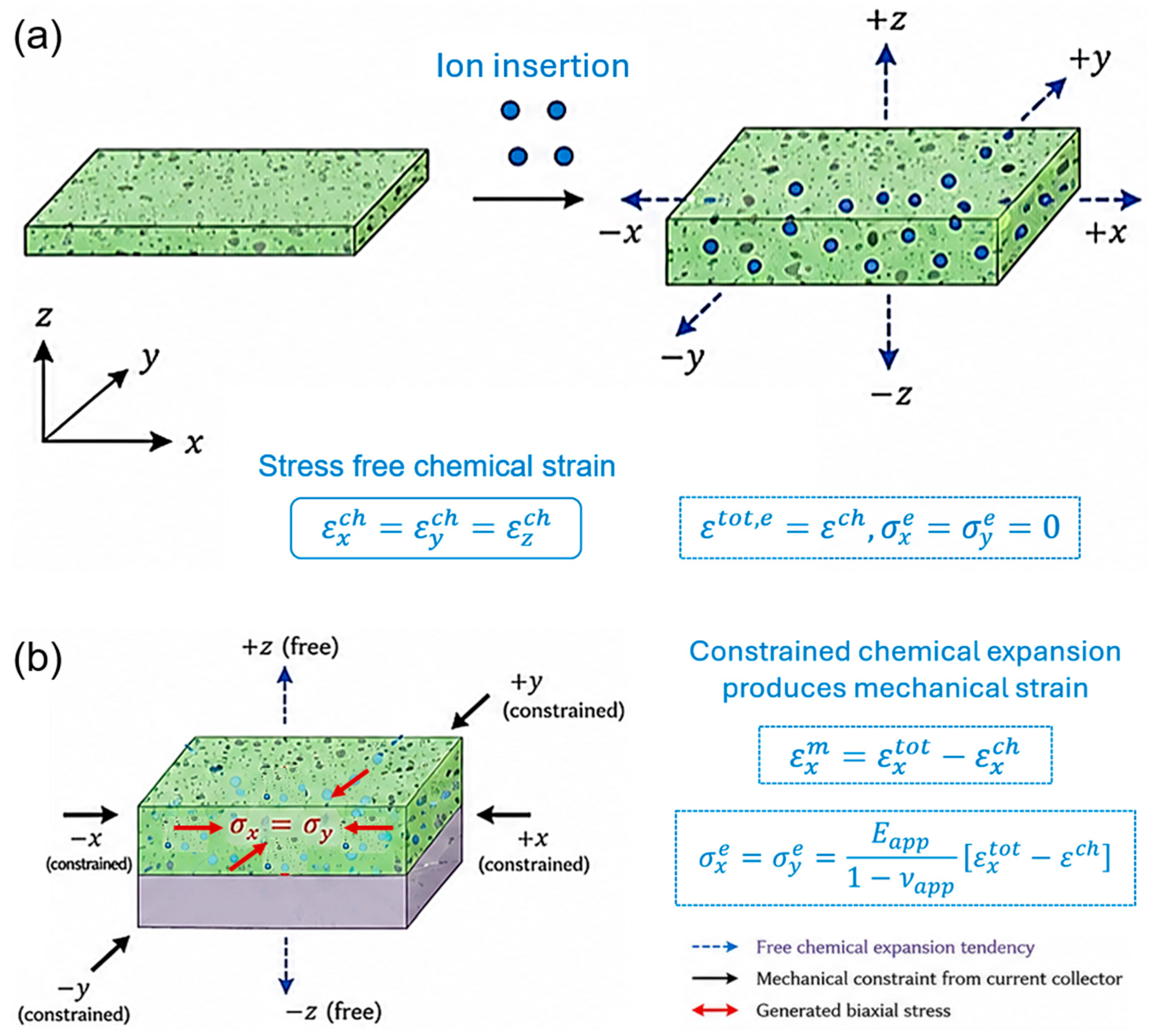
In a freestanding electrode, as shown in Figure 1a, ion insertion induces an unconstrained chemical expansion. For an isotropic electrode, this expansion can be described by equal linear chemical strains in the three principal directions, namely
. (1-6)
The in-plane chemical strain can be experimentally measured using a Digital Image Correlation (DIC)-based approach. In practical electrodes, however, the active composite layer is bonded to a current collector, as illustrated in Figure 1b. The current collector constrains the free in-plane expansion of the electrode, thereby converting part of the chemical strain into mechanical strain and generating biaxial stress within the electrode layer through Equation (1-5). Additional constraints may also arise from stack pressure, cell packaging, or external fixtures, depending on the cell configuration, which are not discussed in present work.
If the electrode/current-collector bilayer is not externally constrained to remain flat, the mismatch strain between the active layer and the current collector may cause bending. In such a bilayer configuration under equi-biaxial deformation assumption, the total in-plane strain at a position through the thickness can be written as
(1-7)
where is the mid-plane or reference-plane strain, is the curvature, and is the coordinate along the thickness direction. The corresponding mechanical strain, , in the electrode is
. (1-8)
Here, the is considered uniform along the z direction and thus not a function of z, as the ion concentration is treated as uniform in the electrode. If the diffusion induced concentration gradient is considered, the should be replaced by , and the concentration profile should be given by solving Fick’s second law.
For isotropic equi-biaxial deformation, the stress in the electrode layer is therefore given by
(1-9)
This formulation provides a direct link between the experimentally measured chemical strain of a freestanding electrode and the stress generated in a practical electrode constrained by a current collector.
It also provides the basis for evaluating the strain energy density of the ion inserted electrode, which can be expressed as
. (1-10)
For the isotropic equi-biaxial case, this becomes
, (1-11)
where . This strain energy represents the elastic mechanical energy stored in the constrained electrode due to electrochemically induced expansion.
Figure 1.
Schematic illustration of (a) stress-free chemical strain generation in a freestanding electrode during ion insertion; (b) stress generation in a practical composite electrode bonded to a current collector, where the electrochemically induced expansion is mechanically constrained.
Figure 1.
Schematic illustration of (a) stress-free chemical strain generation in a freestanding electrode during ion insertion; (b) stress generation in a practical composite electrode bonded to a current collector, where the electrochemically induced expansion is mechanically constrained.
II. A Framework for Estimating the Apparent Young’s Modulus of Composite Electrodes and Inverse Identification of the Young’s Modulus of Active Materials
2.1. Estimation of the Apparent Young’s Modulus of Composite Electrodes Using Hashin-Shtrikman Bounds and Gibson-Ashby Porosity Correction
The porous composite electrode is considered as a two-level heterogeneous material. The first level is a dense solid skeleton composed of active material, conductive additive, and binder, and the second level introduces the porosity into the solid skeleton. The elastic modulus of the dense solid skeleton is estimated using Hashin-Shtrikman (HS) bounds [26], and then, the effect of porosity is delt with a Gibson-Ashby-type relative density correction [27].
The overall procedure can be expressed as
(2-1)
where , , , and are the mass, density, Young’s modulus, and Poisson’s ratio of phase , respectively. The subscripts denote the active material, conductive additive, and binder, respectively. is the volume fraction of each phase. and mean the bulk modulus and shear modulus of phase . and indicate the Hashin-Shtrikman-type estimates for the bulk modulus and shear modulus of the dense solid skeleton, respectively, where means the upper and lower bounds. The quantities denote the upper and lower estimates of the Young’s modulus of the dense solid skeleton, while denote the corresponding apparent modulus of the whole porous electrode.
The true volume of each solid constituent is calculated from its mass and density as
(2-2)
The total volume of the dense solid skeleton phase is therefore
(2-3)
The volume fraction of each phase within the dense solid skeleton, excluding the pore phase, is defined as
(2-4)
and The Hashin-Shtrikman formulation is used to estimate the bounds of the modulus of the dense solid skeleton. The Hashin-Shtrikman bounds provide rigorous variational upper and lower bounds for the effective elastic moduli of statistically isotropic multiphase composites. Compared with the Voigt and Reuss estimates, the Hashin-Shtrikman bounds are generally much narrower and more suitable for estimating the elastic properties of heterogeneous solid electrodes in the absence of detailed microstructural information.
Assuming each solid constituent to be isotropic and linearly elastic, the elastic constants , bulk modulus and shear modulus , of phase are converted according to
(2-5a)
(2-5b)
And then we have
. (2-6)
If the Poisson’s ratios are not experimentally available, reasonable estimates should be adopted. For example, typical values may be 0.2~0.3 for carbonaceous active materials and conductive carbon, and 0.35~0.45 for PVDF-type polymer binders.
For a multiphase isotropic composite, the Hashin-Shtrikman-type estimate for the bulk modulus can be written as 26
(2-7)
where and are the reference bulk and shear moduli. It is clear that is factually only related to .
The corresponding expression for the shear modulus is 26
(2-8)
where
. (2-9)
It can be seen that is related to both and through .
For the upper estimate, the reference phase is selected as the stiffest phase:
(2-10)
Accordingly, the upper Hashin-Shtrikman estimate for the bulk modulus is
(2-11)
and the upper estimate for the shear modulus is
(2-12)
Similarly, for the lower estimate, the reference phase is selected as the most compliant phase:
(2-13)
The lower Hashin-Shtrikman estimate for the bulk modulus is therefore
(2-14)
and the lower estimate for the shear modulus is
(2-15)
The corresponding upper and lower estimates of the Young’s modulus of the dense solid skeleton are calculated by converting and back to Young’s modulus through Equation (2-6), and we have
(2-16a)
(2-16b)
Thus, the Young’s modulus of the dense solid skeleton is bounded by
(2-17)
If a single representative value is required, the arithmetic mean of the two bounds may be used:
(2-18)
After determining the modulus of the dense solid skeleton, the effect of porosity is introduced using a Gibson-Ashby-type scaling relation. The porosity of the porous electrode is defined as the ratio between the pore volume and the total porous electrode volume:
(2-19)
If the total electrode volume is known from the electrode area and thickness ,
(2-20)
then the porosity is calculated as
(2-21)
or explicitly,
(2-22)
Alternatively, if the electrode density is known, the electrode volume can be written as
(2-23)
and the porosity becomes
(2-24)
According to Gibson-Ashby scaling relation, for a porous solid, the apparent Young’s modulus is related to the relative density by 27
(2-25)
where is the apparent modulus of the porous electrode, is the apparent density of the porous electrode, is the density of the dense solid skeleton, is a structural coefficient, and is a porosity-dependent scaling exponent.
Since the relative density of the porous electrode is
(2-26)
the Gibson-Ashby relation becomes
(2-27)
Using the Hashin-Shtrikman upper and lower estimates for , the corresponding bounds of the apparent electrode modulus are
(2-28)
(2-29)
Therefore, the apparent Young’s modulus of the porous composite electrode is estimated as
(2-30)
The parameters, and depend on pore morphology, pore connectivity, calendering history, particle packing, and binder distribution. For quantitative prediction, and should be calibrated using measured moduli of electrodes with different porosities or compaction densities.
When no experimental calibration is available, a common first approximation is to set and to choose For an initial estimate, one may take Then the single-value estimate of the apparent modulus can then be approximated by
(2-31)
More generally, one may use
(2-32)
Combining the Hashin–Shtrikman bounds with the Gibson–Ashby porosity correction gives
(2-33)
Here,
(2-34)
and
(2-35)
For the upper estimate,
(2-36)
whereas for the lower estimate,
(2-37)
The above modeling provides a closed-form framework for estimating the apparent elastic modulus of a porous composite electrode using constituent masses, densities, elastic moduli, Poisson’s ratios, and electrode porosity.
2.2. Inverse Estimation of the Active Particle’s Young’s Modulus from the Apparent Modulus of Porous Composite Electrodes
When the apparent modulus of the porous electrode and the moduli of the conductive agent and binder are known, the Young’s modulus of the active particles can be estimated inversely. This is important when the modulus of the active particles varies with ion concentration and direct measurement is difficult.
Because the electrode is a heterogeneous porous medium and its microstructure is generally not explicitly resolved, the inverse problem is generally not unique. Here, the active particle Young’s modulus is therefore identified as an admissible interval rather than a single deterministic value. The forward model in Section 2.1 combines Hashin–Shtrikman bounds for the dense solid skeleton with a Gibson–Ashby-type porosity correction. The inverse problem is formulated by finding the range of active-particle moduli for which the measured apparent electrode modulus lies within the predicted upper and lower bounds.
The proposed inverse framework can be summarized as
(2-38)
where is the experimentally measured apparent Young’s modulus of the porous electrode, is the equivalent dense-skeleton modulus inferred from the porosity correction, and and are the Hashin–Shtrikman lower and upper estimates of the dense solid skeleton modulus as functions of the unknown active particle modulus . The apparent Young’s modulus of the porous electrode is described by
(2-39)
The active particle modulus is treated as the unknown parameter, while the properties of the conductive additive and binder are assumed to be known.
For the active material, the bulk modulus and shear modulus are functions of the unknown active particle Young’s modulus :
(2-40)
(2-41)
For the conductive additive and binder, the elastic constants are known:
(2-42)
(2-43)
Therefore, the set of phase moduli entering the Hashin–Shtrikman model is
(2-44a)
(2-44b)
The Hashin–Shtrikman bounds provide upper and lower estimates of the effective bulk and shear moduli of a statistically isotropic multiphase composite.
For a given reference phase with bulk modulus and shear modulus , the Hashin–Shtrikman estimate of the bulk modulus is given as
, (2-45)
and the Hashin–Shtrikman estimate of the shear modulus is
(2-46)
For the upper estimate, the stiffest reference phase is used:
(2-47)
(2-48)
where
(2-49)
(2-50)
The upper Hashin–Shtrikman estimate of the bulk modulus is then given by
(2-51)
and the upper Hashin–Shtrikman estimate of the shear modulus is
(2-52)
For the lower estimate, the most compliant reference phase is used:
(2-53)
(2-54)
where
(2-55)
(2-56)
The lower Hashin–Shtrikman estimate of the bulk modulus is given by
(2-57)
and the lower Hashin–Shtrikman estimate of the shear modulus is
(2-58)
The corresponding upper and lower Young’s moduli of the dense solid skeleton are obtained from
(2-59)
(2-60)
Therefore, for a given active particle modulus , the dense solid skeleton modulus satisfies
(2-61)
According to the Gibson–Ashby relation, the measured apparent modulus of the porous electrode follows
(2-62)
Thus, the dense skeleton modulus required to reproduce the measured apparent modulus is
(2-63)
This quantity represents the effective modulus that the dense solid skeleton would need to have in order to produce the measured porous electrode modulus under the assumed Gibson–Ashby porosity correction.
Instead of imposing a single equality between the predicted and measured modulus, the inverse problem is formulated using the Hashin–Shtrikman bounds. For a physically admissible active particle modulus , the target dense skeleton modulus must lie between the lower and upper Hashin–Shtrikman estimates, that is
(2-64)
Substituting
(2-65)
one obtains the inverse admissibility condition:
(2-66)
Equivalently, in terms of the apparent modulus,
(2-67)
Therefore, the admissible active particle modulus set is defined as
(2-68)
If the admissible set is connected, it can be written as
(2-69)
This interval represents the range of active particle Young’s moduli that are consistent with the measured apparent electrode modulus under the assumed Hashin–Shtrikman–Gibson–Ashby framework.
In most practical electrode systems, the predicted skeleton moduli and increase monotonically with the active-particle modulus . Under this monotonicity assumption, the bounds of the admissible active particle modulus interval can be obtained by solving two scalar nonlinear equations.
The lower bound is obtained from the upper Hashin–Shtrikman estimate:
(2-70)
Equivalently,
(2-71)
The upper bound is obtained from the lower Hashin–Shtrikman estimate:
(2-72)
Equivalently,
(2-73)
Thus,
(2-74)
and
(2-75)
Because
(2-76)
the modulus required to match the experimental value is reached at a smaller when the upper Hashin–Shtrikman estimate is used, and at a larger when the lower estimate is used. Therefore,
(2-77)
The final inverse estimate is
(2-78)
with
(2-79)
and
, (2-80)
provided that the inverse functions exist in the considered modulus range .
The two boundary equations can be solved numerically by defining residual functions. For the lower bound of the active particle modulus, the residual is
(2-81)
The root of this equation gives
(2-82)
For the upper bound of the active particle modulus, the residual is
(2-83)
The root of this equation gives
(2-84)
Alternatively, using the target dense skeleton modulus,
(2-85)
(2-86)
The roots are
(2-87)
(2-88)
The use of the target dense skeleton modulus is often numerically convenient because the porosity correction is applied only once. Solving Equations (2-82) and (2-84) or (2-87) and (2-88) gives the and , respectively. The lower bound corresponds to the case where the solid skeleton is assumed to achieve the upper Hashin–Shtrikman estimate. In this case, a smaller active particle modulus is sufficient to reproduce the measured apparent electrode modulus. In contrast, the upper bound corresponds to the case where the solid skeleton follows the lower Hashin–Shtrikman estimate. Because the lower bound predicts a more compliant skeleton, a larger active-particle modulus is required to match the same measured apparent electrode modulus.
A feasible solution exists only if the target dense skeleton modulus lies within the range spanned by the Hashin–Shtrikman bounds over the prescribed search interval. Let the search interval be
(2-89)
A solution for exists if
(2-90)
Similarly, a solution for exists if
(2-91)
If either condition is not satisfied, the corresponding root does not exist within the assumed search interval.
Although the interval-based inverse formulation is more physically appropriate, one may also define a representative skeleton modulus as the arithmetic mean of the Hashin–Shtrikman bounds:
(2-92)
A single equivalent active particle modulus can then be obtained by solving
(2-93)
This value should not be interpreted as the unique intrinsic modulus of the active material. Rather, it should be regarded as a model-calibrated effective modulus.
The inverse estimate is highly sensitive to the porosity correction. Since small changes in , , or may produce large variations in the inferred active-particle modulus. Consequently, if possible, and should be calibrated using experimental modulus data from electrodes with different porosities or compaction densities.
III. Mechanical Work and Elastic Strain Energy of a Substrate-Constrained Electrode During Ion Insertion with Concentration-Dependent Thickness and Modulus
3.1. Mechanical Description of the Constrained Electrode Layer
We first consider a freestanding electrode. The ion insertion induces a stress-free chemical expansion of the electrode film, and ions are treated as uniformly distributed in the active electrode film. The corresponding free linear chemical strain is denoted by
where represents the ion concentration or state of charge.
Since the active electrode film was freestanding, it will expand freely by in all directions under isotropic chemical expansion. However, in a practical electrode, the active layer is bonded to a current collector, and its in-plane expansion is mechanically constrained, which is the situation we considered in the following discussion.
We denote the actual in-plane strain of the active layer of the substrate constrained electrode under equi-biaxial assumption by
For isotropic active electrode layer, we have
The in-plane mechanical strain of the active layer is therefore given by
, (3-1)
where indicates that the active layer is under in-plane compression.
For a sufficiently thick and stiff current collector, the in-plane deformation of the active layer may be approximated as fully constrained:
(3-2)
In this rigid-current-collector limit,
. (3-3)
3.2. Concentration-Dependent Biaxial Modulus of the Active Layer and In-Plane Stress
The active layer is assumed to be isotropic and linearly elastic at each ion concentration. Both Young’s modulus and Poisson’s ratio may depend on concentration, i.e.,
(3-4)
(3-5)
Here, the and are equivalent to the apparent modulus and Poisson’s ratio of the composite electrode. In the following, we use the subscript e to replace the subscript app for simplicity. The concentration-dependent biaxial modulus of the active layer is defined as
. (3-6)
Under plane-stress conditions,
(3-7)
and under equi-biaxial in-plane deformation,
(3-8)
The in-plane stress in the active layer is therefore
(3-9)
or explicitly,
. (3-10)
In the rigid current collector limit, and hence
. (3-11)
The negative sign denotes compressive stress in the active layer during ion insertion.
3.3. Out-of-Plane Strain and Thickness Evolution
Although the active layer is under plane stress, the out-of-plane strain is generally nonzero. The elastic out-of-plane Poisson strain is given by
(3-12)
Since we have
(3-13)
Substituting Equation (3-10) into Equation (3-13) gives
. (3-14)
The total out-of-plane strain of the constrained active layer contains two contributions, i.e., the free chemical expansion strain, , and the elastic Poisson strain, . Therefore,
. (3-15)
The active electrode layer thickness is then written as
. (3-16)
where is the initial active electrode layer thickness.
Substituting Equation (3-15) into Equation (3-16), we have
. (3-17a)
or equivalently,
. (3-17b)
Equation (3-17) shows that the thickness evolution of the electrode layer depends directly on
(3-18)
Since may itself depend on through force balance with the current collector, the thickness can also depend indirectly on .
3.4. Rigid Current Collector Limit
If the current collector is sufficiently thick and stiff, the active layer in-plane strain is approximately zero, i.e.,
(3-19)
Equation (3-15) then becomes
(3-20)
Thus,
, (3-21)
and the active layer thickness becomes
. (3-22)
In this rigid substrate approximation, the thickness variation is governed by and . The modulus does not explicitly enter Equation (3-22), because the in-plane strain has already been prescribed as zero. However, the stress still depends directly on :
. (3-23)
3.5. Finite-Stiffness Current Collector: Coupled Dependence of
onWhen the current collector is not treated as perfectly rigid, the active layer and the current collector deform together. Perfect bonding requires in-plane strain compatibility:
(3-24)
The current collector is assumed to have no lithiation-induced chemical strain. Its stress is therefore
, (3-25)
where
(3-26)
is the biaxial modulus of current collector.
The active electrode layer stress is
. (3-27)
Neglecting bending and assuming no external in-plane force, force balance per unit width gives
, (3-28)
where is the initial thickness of the current collector and is treated as constant. Noting that the variation in induced by the elastic Poisson strain in the current collector is neglected.
Substituting Equations (3-25) and (3-27) into Equation (3-28) yields
(3-29)
Solving Equation (3-29) for gives
(3-30)
Equation (3-30) shows explicitly that the actual in-plane strain depends on the concentration-dependent modulus .
Since is given by Equation (3-17b), Equations (3-17b) and (3-30) form a coupled system:
Therefore, in the finite-stiffness current collector case, the thickness depends on indirectly through .
For compactness, we define in-plane extensional stiffness per unit width of the current collector
, (3-33)
and Poisson coupling factor
. (3-34)
Then, Equation (3-31) can be written as
(3-35)
Substituting Equation (3-30) into Equation (3-35) gives an implicit equation for . This equation can be rearranged into a quadratic form:
. (3-36)
The physically meaningful positive solution is
. (3-36)
Equation (3-36) explicitly shows that, when the current collector has finite stiffness, the active layer thickness depends on the concentration-dependent modulus through . As long as the and are explicitly known, the can be obtained by Equation (3-36).
After obtaining , the in-plane strain is calculated from
(3-37)
and the in-plane stress in the active electrode layer follows from
. (3-38)
On the other hand, if is unknown while can be treated as known and constant, and if and are measured experimentally, then and can be calculated by solving Equations (3-31) and (3-32) simultaneously. This is important for the practical application of the model, as and can be experimentally measured through carefully designed DIC-based in situ electrochemical tests.
3.6. Elastic Strain Energy Density
The elastic strain energy density in the active electrode layer under plane-stress conditions is
. (3-39)
For equi-biaxial deformation, , and therefore
. (3-40)
Using Equation (3-9) or (3-10), we have
, (3-41)
or
. (3-42)
The out-of-plane strain does not appear explicitly in Equation (3-42) because . However, it will affect the total strain energy through the current active layer thickness .
3.7. Elastic Strain Energy of the Active Electrode Layer
The elastic strain energy stored in the active electrode layer can be obtained by integrating the strain energy density over the current volume of the active electrode layer :
. (3-43)
Assuming uniform stress and strain in the active layer, the energy per unit projected electrode area is
, (3-44)
or
. (3-45)
For the rigid current collector case,
and ,
thus, we have
, (3-46a)
or
. (3-46b)
For the finite-stiffness current collector case, should be obtained from Equation (3-36), and then substituted into Equation (3-45).
When the elastic energy stored in the current collector is also included, the total strain energy becomes
. (3-47)
Equation (3-47) accounts for both the compressive elastic energy stored in the active layer and the tensile elastic energy stored in the current collector.
3.8. Mechanical Work Generated During Ion Insertion
The incremental mechanical work associated with the constrained chemical expansion is
. (3-48)
Under equi-biaxial in-plane deformation, , and , then we have
. (3-49a)
For rigid current collector conditions, i.e., , then we have
. (3-49b)
The incremental work per unit projected area is therefore given by
. (3-50)
Integrating from the initial state (e.g., ) to , the total mechanical work per unit projected area is
. (3-51)
Substituting Equation (3-27) into Equation (3-51) gives
(3-52)
or explicitly,
, (3-53)
with
. (3-54)
Equation (3-53) is the recommended general expression for the mechanical work when both and are concentration dependent. This expression should be used when the current collector is much stiffer than the active electrode layer and the active layer thickness variation is non-negligible.
For a current collector with finite stiffness, is generally not zero or constant, thus the mechanical work must be calculated from the general incremental relation
, (3-55)
and
, (3-56)
using .
The total mechanical work is then given by
, (3-57)
or equivalently,
, (3-58)
with . (3-59)
Defining , (3-60)being a dimensionless in-plane strain accommodation factor characterizing the fraction of the chemical expansion strain that is accommodated by the in-plane total deformation of the electrode, then the in-plane total strain can be written compactly as
. (3-61)
Accordingly, the elastic mismatch strain becomes
, (3-62)
and its derivative with respect to concentration is
. (3-63)
Substituting Equations (3-61) and (3-63) into the general work formula (3-58) yields the more explicit form
, (3-64)
where and can be obtained from the coupled equations (3-31) and (3-32)
The rigid current collector case can be recovered automatically as a limiting case of the finite-stiffness formulation. In the limit of infinitely large current collector stiffness,
, (3-65)
we have
(3-66)
Substituting Equations (3-65) and (3-66) into (3-64) gives
, (3-67)
which is exactly the same as the previously derived expression for the rigid current collector case Equation (3-53).
3.9. Difference Between Accumulated Mechanical Work and Final Elastic Strain Energy
When , , and are independent of concentration, the accumulated mechanical work may reduce to the final elastic strain energy. For example, for a rigid current collector, Equation (3-54)
will reduce to Equation (3-46b)
.
However, when , , and are dependent of concentration
and the process work and final stored elastic energy are generally different.
The accumulated work is a path integral,
,
whereas the final elastic energy is a state function,
.
The difference arises because the elastic modulus, Poisson’s ratio, thickness, and constraint state may all evolve during ion insertion.
IV. A General Framework for Estimating Stress in an Active Electrode Film–Current Collector Bilayer from Curvature Evolution Under the Assumption of Spatially Uniform Concentration
During electrochemical cycling, ion insertion and extraction induce volumetric changes in the active electrode film. Because the active film is bonded to the current collector, its free chemical expansion is mechanically constrained by the current collector, resulting in an elastic strain mismatch between the two layers. In the absence of external constraints along the thickness direction, this mismatch can induce bending deformation of the bilayer electrode and lead to curvature evolution during cycling.
To determine the stress and apparent Young’s modulus of the active electrode film during cycling, we develop a mechanical model for a bilayer structure composed of an active electrode film and a current collector. The model couples the evolution of the active electrode thickness with experimentally measured curvature and chemical strain. The following assumptions are adopted: both layers are isotropic and linearly elastic, the in-plane stress state is equi-biaxial, the ion concentration is spatially uniform within the active electrode, and the active layer is perfectly bonded to the current collector so that strain compatibility is maintained at the interface.
The interface between the current collector and the active layer is taken as the reference plane of the bilayer system, with . A Cartesian coordinate system is established with the -axis normal to the electrode plane and the - and -axes lying within the reference plane, as illustrated in Figure 2. The active electrode occupies the region , while the current collector occupies , where is the thickness of the current collector and is the active electrode thickness at ion concentration . The initial active electrode thickness is denoted by .
A positive curvature is defined such that the in-plane total strain increases with increasing . Therefore, according to classical beam or plate theory, the in-plane total strain varies linearly through the thickness as
, (4-1)
where is the in-plane strain at the reference plane . Under the assumption of spatially uniform ion concentration, the intrinsic in-plane chemical strain of the active electrode, , is independent of . The mechanical strain in the active electrode and the strain in the current collector are therefore given by
(4-2)
Here, denotes the elastic or mechanical in-plane strain in the active electrode, namely the difference between the total in-plane strain and the free chemical strain.
For an equi-biaxial plane stress state, the in-plane stresses in the active electrode and current collector are
(4-3)
where
(4-4a)
(4-4b)
Here, and are the concentration-dependent effective Young’s modulus and Poisson’s ratio of the active electrode, respectively, while and are the Young’s modulus and Poisson’s ratio of the current collector.
Although the active electrode is assumed to be under plane stress, its out-of-plane strain is generally nonzero. Under equi-biaxial plane stress, the elastic out-of-plane Poisson strain in the active electrode is
. (4-5)
Substituting Equation (4-3) into Equation (4-5) gives
. (4-6)
Assuming isotropic chemical expansion of the active material, the free out-of-plane chemical strain is equal to the free in-plane chemical strain,
(4-7)
The total out-of-plane strain of the constrained active electrode therefore consists of the free chemical expansion strain and the elastic Poisson strain. Since the elastic Poisson strain varies through the thickness, we approximate the thickness evolution using the thickness-averaged out-of-plane strain. To first order in strain, the average elastic Poisson strain is evaluated over the initial electrode thickness as
. (4-8)
Substituting Equation (4-6) into Equation (4-8) yields
. (4-9)
Therefore, the thickness-averaged total out-of-plane strain of the active electrode is
, (4-10)
or equivalently,
. (4-11)
The active electrode thickness during ion insertion is then estimated as
. (4-12)
Substituting Equation (4-11) into Equation (4-12), we obtain
. (4-13)
As the system is not subjected to any external forces or external bending moments, it must satisfy the conditions of both force and moment equilibrium [28]:
, (4-14)
and
. (4-15)
Substituting Equation (4-3) into Equations (4-14) and (4-15) gives the force equilibrium equation
, (4-16)
and the moment equilibrium equation
. (4-17)
Equations (4-13), (4-16), and (4-17) constitute a coupled system for determining the active electrode thickness, the reference-plane strain, and the concentration-dependent effective modulus of the active electrode. Specifically, if , , , , and are known, and if and are experimentally measured, the unknowns , , and can be determined. Once these quantities are obtained, the stress distributions in both the active electrode and the current collector can be calculated using Equation (4-3).
In practice, can be obtained from in situ curvature measurements, while can be determined from independent chemical strain measurements, for example by digital image correlation or by measurements on unconstrained electrodes.
The framework above is based on elastic deformation. Experimentally, the validity of the elastic assumption can be assessed by comparing the strain paths during ion insertion and extraction. If the deformation is elastic, the strain path during extraction should retrace that during insertion at the same ion concentration. In this case, the absolute strain change rates during insertion and extraction should be identical at a given concentration. Any residual deformation should be attributable only to trapped ions or irreversible compositional changes in the active material.
During the initial cycles of a battery, however, electrolyte decomposition and other irreversible side reactions may occur. These reactions can form by-products such as the solid-electrolyte interphase on the active material surface, leading to inelastic deformation of the electrode. Therefore, for practical stress and modulus estimation, the end state of the first cycle may be used as a reference state, provided that most irreversible side reactions have been completed and the subsequent cycles are dominated by elastic deformation.
For a simplified data-reduction procedure, the reference plane at the current collector/electrode interface may be approximated as the neutral plane if the neutral axis is sufficiently close to the interface. Under this additional approximation,
. (4-18)
This approximation should be used only when justified by the relative stiffnesses and thicknesses of the two layers. With , Equation (4-2) reduces to
(4-19)
The corresponding simplified expression for the active electrode thickness becomes
. (4-20)
The thickness-averaged mechanical strain in the active electrode and the thickness-averaged strain in the current collector are obtained by averaging Equation (4-19) over each layer. Thus, we have
, (4-21a)
and
. (4-21b)
The negative sign in Equation (4-21b) follows directly from the adopted coordinate system, where the current collector lies in the region .
At the end of the first cycle, the electrode generally does not return to its initial stress-free state. Let the residual average stress in the active electrode at this state be denoted by , the corresponding curvature by , and the electrode thickness by . The thickness-averaged stress in the Cu current collector at the end of the first cycle is
. (4-22)
The force balance per unit width requires
. (4-23)
Substituting Equation (4-22) into Equation (4-23) gives
. (4-24)
Therefore, the residual average stress in the active electrode at the end of the first cycle is
. (4-25)
From the second cycle onward, the electrode deformation is assumed to be predominantly elastic. Let the average stress in the active electrode at concentration be denoted by . The force balance becomes
. (4-26)
Using Equation (4-21b), the average stress in the current collector is
. (4-27)
Therefore, Equation (4-26) gives
. (4-28)
If the active electrode thickness remains approximately constant after the first cycle, i.e., , then subtracting Equation (4-24) from Equation (4-28) yields
. (4-29)
Equivalently,
. (4-30)
Equation (4-30) provides a practical means of estimating the average stress in the active electrode during the second and subsequent cycles from the measured curvature change relative to the first-cycle reference state.
The apparent modulus of the active electrode can then be estimated from the relationship between the average stress and the average mechanical strain. Using Equation (4-21a), the average mechanical strain in the active electrode is
. (4-31)
Taking the end of the first cycle as the reference state, the stress increment and mechanical strain increment are defined as
, (4-32)
and
. (4-33)
Because the electrode is a porous composite and its stress–strain response may be nonlinear, an apparent biaxial modulus can be estimated using the chord modulus method:
. (4-34)
The corresponding apparent Young’s modulus is then
. (4-35)
Here, should be interpreted as a concentration-dependent apparent or effective Young’s modulus of the composite active electrode, rather than the intrinsic Young’s modulus of the active material particles.
V. An Inverse Chemo-Mechanical Framework for Diffusion-Induced Stress in Substrate-Constrained Electrodes Under Single-Step Galvanostatic Ion Insertion and Extraction: Independent Inversion of for Ion Insertion and Extraction
5.1. Physical System
We consider a planar film electrode of thickness , perfectly bonded to a current collector/substrate of thickness . A Cartesian coordinate is introduced along the thickness direction, with at the electrode/substrate interface, at the electrochemically active free surface of the electrode, and in the current collector. Since the in-plane dimensions are much larger than the thickness, edge effects are neglected and the problem is treated as one-dimensional in the thickness direction. The film electrode is assumed to deform within the regime of small strains and linear elasticity. For simplicity, the electrode material is taken as isotropic, with isotropic diffusion and isotropic chemical swelling. Meanwhile, the chemical diffusion coefficient and the electrode thickness are assumed to be constant and independent of concentration.
Because the electrode is bonded to a substrate, free in-plane expansion or contraction of the film is suppressed during ion insertion and extraction. As a result, concentration changes generate a mismatch between the natural chemical swelling strain of the electrode and the actual kinematically admissible deformation, which gives rise to in-plane stress. The top surface of the film is traction-free, so that the out-of-plane normal stress is negligible compared with the in-plane stress. Under these assumptions, the electrode develops an equi-biaxial in-plane stress state,
(5-1)
The ion concentration satisfies the one-dimensional Fickian diffusion equation in the active electrode [29],
(5-2)
where is the ion concentration and is the chemical diffusion coefficient.
In the present formulation, ion insertion and ion extraction are analyzed independently. For insertion experiments, all datasets are assumed to start from the same initial concentration . For extraction experiments, all datasets are assumed to start from the same initial concentration . These two initial concentrations may be different, depending on the experimental protocol.
For insertion,
(5-3a)
For extraction,
(5-3b)
Only the outer surface is assumed to be electrochemically active, while the substrate interface is impermeable. Accordingly,
(5-4)
At the active surface, the imposed current density prescribes the ion molar flux. Let denote the applied current density, the number of electrons transferred per ion, and Faraday’s constant. The interfacial molar flux is
(5-5)
In present case, we use lithium as an example, and thus . The ion insertion means lithiation and the ion extraction means delithiation.
The sign convention is chosen such that denotes inward lithium flux into the electrode during charging/lithiation. The electrochemical boundary condition at is therefore
(5-6)
For lithiation,
(5-7a)
whereas for delithiation,
(5-7b)
Side reactions, interfacial kinetic limitations, concentration losses due to parasitic processes, and electrode thickness variation due to lithium insertion/extraction are neglected. Thus, the applied current is assumed to be fully converted into lithium insertion/extraction at the active surface. If both surfaces were electrochemically active, the second boundary condition would have to be modified accordingly; that case is not considered here.
The thickness-averaged concentration is defined as
(5-8)
Integrating the diffusion equation over the film thickness gives
(5-9)
Therefore, for a constant galvanostatic flux,
(5-10)
where for lithiation and for delithiation.
It should be emphasized that Eq. (5-10) gives only the thickness-averaged concentration. Because lithium concentration is generally nonuniform through the electrode thickness, the local concentration may be larger or smaller than the average value, especially at high current density or small diffusivity. Therefore, the concentration interval over which the local modulus function is identified should be determined from the local concentration field rather than from the averaged concentration alone.
Solving the diffusion equation under the above initial and boundary conditions gives
(5-11)
Here should be interpreted as the initial concentration of the independently analyzed experiment group. Specifically, for lithiation datasets and for delithiation datasets.
For subsequent inverse identification, the concentration interval sampled by the experiments must be defined separately for lithiation and delithiation. In lithiation experiments with , the local concentration generally increases with time, and the maximum concentration is typically attained near the end of the experiment and close to the electrochemically active surface. In delithiation experiments with , the local concentration decreases with time, and the minimum concentration is typically attained near the end of the experiment and close to the electrochemically active surface.
5.2. Curvature and Constitutive Relation for Stress
Lithium insertion or extraction produces a local stress-free volumetric expansion or contraction in a freestanding electrode. This response is described by an isotropic chemical strain,
(5-12)
where is the coefficient of compositional expansion, is the reference concentration for the considered experiment group, and is the Kronecker delta. For lithiation, ; for delithiation, . Physically, represents the linear strain per unit change in lithium concentration and can be estimated experimentally from strain measurements during low-rate lithiation/delithiation or after relaxation [30].
In the electrode/substrate bilayer structure, because the electrode film is perfectly bonded to the substrate, in-plane expansion or contraction is constrained. This constraint generates in-plane stress: generally compressive during lithiation and tensile during delithiation. If the bilayer is free to bend, this stress drives curvature evolution.
Within classical beam theory, the in-plane strain varies linearly across the thickness. The in-plane mechanical strains in the active electrode and current collector are written as [31]
(5-13a)
(5-13b)
where is the in-plane strain at the electrode/current collector interface and is the curvature [32]. With the convention , positive means that the in-plane strain increases from the current collector side to the electrode surface side.
The biaxial modulus is defined as
(5-14)
where is Young’s modulus and is Poisson’s ratio.
The current collector is assumed to have a constant biaxial modulus . In contrast, the biaxial modulus of the active electrode, which is factually the apparent biaxial modulus of the active electrode, generally depends on lithium concentration. Thus,
. (5-15)
The equi-biaxial stresses in the active electrode and current collector are therefore [33]
(5-16a)
(5-16b)
In the absence of external mechanical loading, force and moment balance require [28]
(5-17a)
(5-17b)
To express the governing equations compactly, the stiffness moments of the active layer are defined as
(5-18)
and the chemical loading moments as
(5-19)
Substitution into the force and moment balance equations gives
(5-20a)
(5-20b)
Equivalently,
(5-21)
where
(5-22a)
(5-22b)
(5-22c)
Thus, for a prescribed constitutive relation , the curvature predicted by the variable-modulus model is
(5-23)
This equation defines the forward operator that maps the modulus-concentration relation to the curvature response,
(5-24)
Once and are obtained, the local stress distribution follows directly from Eqs. (5-16a) and (5-16b). The average stress in the active electrode is
(5-25)
or equivalently,
(5-26)
The maximum absolute stress in the active electrode is evaluated as
(5-27)
Because varies through the thickness, the maximum stress does not necessarily occur at or .
5.3. Independent Inverse Identification of Modulus from Measured Curvature
In principle, if the curvature history is measured in situ, Eq. (5-23) can be used to identify the unknown modulus-concentration relation . However, direct pointwise recovery of from curvature data is generally ill-posed. The curvature at each time is a scalar quantity, whereas is an unknown continuous function. Moreover, the curvature response depends on through the thickness-weighted integrals , , , , and . Consequently, different functions may produce nearly indistinguishable curvature histories.
To address this non-uniqueness, a two-step inverse identification strategy is adopted. First, an apparent homogeneous modulus is extracted from the experimental curvature data using an effective-constant-modulus approximation. This reduced-order identification provides the magnitude and trend of the modulus evolution. Second, the inferred apparent modulus-concentration trend is used to guide the choice of candidate functional forms for . Finally, the full variable-modulus model is used to identify a more accurate local modulus-concentration relation through parameterized and, when necessary, regularized inverse analysis.
In the present work, lithiation and delithiation experiments are analyzed independently. For lithiation, all experiments are assumed to start from the same initial concentration , and the applied flux satisfies . Multiple lithiation experiments at different current densities are jointly fitted using a common modulus function
(5-28a)
For delithiation, all experiments are assumed to start from the same initial concentration , and the applied flux satisfies . Multiple delithiation experiments are jointly fitted using a separate modulus function
(5-28b)
No constraint is imposed that and must be identical, unless fully reversible elastic behavior without path dependence, hysteresis, damage, or irreversible structural change is assumed.
Step I: Apparent modulus identification using an effective constant modulus
Strictly, because the lithium concentration varies through the electrode thickness, the active-layer modulus should be written as . A fully rigorous treatment therefore requires a specified constitutive relation and solution of the equilibrium equations with variable coefficients. To retain analytical tractability in the first stage, the spatially varying modulus field is approximated by an apparent homogeneous modulus at each time,
(5-29)
The quantity should be interpreted as an apparent or effective biaxial modulus that reproduces the measured curvature within the homogeneous-modulus approximation. It is not, in general, identical to the local material function .
With Eq. (5-29), the force and moment balance equations reduce to
(5-30a)
(5-30b)
where
. (5-31)
The sign of is retained in Eq. (5-31). Thus, the same expression applies to both lithiation and delithiation, provided that is used for lithiation and is used for delithiation.
Given the measured curvature , Eqs. (5-30a) and (5-30b) can be solved at each time for the two unknowns and , under the physical constraint
(5-32)
Data points at very early times may be excluded from Step I because the curvature signal is too small to identify the apparent modulus robustly.
For lithiation datasets, this procedure gives
(5-33a)
and for delithiation datasets, it gives
(5-33b)
Using the thickness-averaged concentration,
(5-34)
the apparent modulus history can be converted into an apparent modulus-concentration relation. For lithiation,
(5-35a)
where .
For delithiation,
(5-35b)
where .
These apparent relations provide useful reduced-order descriptors of the macroscopic modulus evolution. If the apparent modulus-concentration relation is approximately linear, a linear or weakly nonlinear model may be used as the initial candidate. If it decreases monotonically and tends to saturate, a saturating exponential model may be particularly appropriate. Logistic, Hill-type, or monotonic spline representations may also be considered when more complex transitions are observed and sufficient data are available.
The apparent relation is used only to guide the subsequent full inversion. It should not be interpreted as the exact local constitutive relation , because the measured curvature is sensitive to thickness-weighted integrals of , rather than to its pointwise value.
Step II: Parameterized full inversion of
In the second step, the local concentration-dependent modulus is represented by a finite-dimensional parameterization. Since lithiation and delithiation are treated as independent inverse problems, two separate functions are introduced:
(5-36a)
for lithiation, and
(5-36b)
for delithiation.
The choice of parameterization is guided by the apparent trends obtained in Step I.
For example, if the apparent modulus is nearly linear, one may use
(5-37)
where or .
If the modulus evolves in an exponential form, a quadratic exponential model may be adopted,
(5-38)
where
(5-39)
Here is the normalized concentration for the independently analyzed process . The normalization range must be determined separately for lithiation and delithiation from the local concentration fields.
For lithiation, , the normalized concentration is defined as
(5-40)
Because all lithiation experiments start from , the lower bound is taken as
(5-41)
For multiple lithiation experiments, , the local concentration field of the -th experiment is
(5-42)
with
(5-43)
The maximum local concentration sampled by all lithiation experiments is
(5-44)
To avoid numerical extrapolation caused by discretization or series truncation errors, a small safety factor is introduced:
(5-45)
Typically, is chosen between 1.01 and 1.05.
For delithiation, , the normalized concentration is defined as
(5-46)
If all delithiation experiments start from , the upper bound can be taken as
(5-47)
For multiple delithiation experiments, , the local concentration field of the -th experiment is
(5-48)
with
(5-49)
The minimum local concentration sampled by all delithiation experiments is
(5-50)
A safety factor is introduced as
(5-51)
Again, is typically chosen between 1.01 and 1.05.
In addition to the quadratic exponential model, a saturating exponential model may be used when the apparent modulus changes rapidly at low lithium concentration and then approaches a plateau. For either lithiation or delithiation, this model is written as
(5-52)
where is the modulus at , is the saturated modulus at high , and is the transition rate. The superscript denotes either lithiation or delithiation.
To guarantee positivity of the parameters, a logarithmic parameterization can be introduced:
(5-53)
The saturating exponential model then becomes
(5-54)
with
(5-55)
More flexible choices, such as B-splines or monotonic splines, may also be used when sufficient experimental data are available.
For a given parameter vector , where or , the local concentration field is first calculated from the analytical diffusion solution. The stiffness and chemical loading moments are then evaluated as
(5-56)
(5-57)
Here
(5-58)
The corresponding stiffness matrix terms are
(5-59a)
(5-59b)
(5-59c)
The predicted curvature is then computed as
(5-60)
To reduce the influence of initial curvature, residual stress, or mounting errors, curvature increments are used:
(5-61)
(5-62)
For lithiation, the objective function of the inverse problem is formulated as
(5-63)
For delithiation, the objective function of the inverse problem is formulated independently as
(5-64)
is a weighting factor, and a useful weighting choice is
(5-65)
where
(5-66)
This weighting balances the contributions from experiments with different numbers of data points and different curvature magnitudes.
For low-dimensional models, such as the linear model, quadratic exponential model, and saturating exponential model, may be omitted. For spline-based representations, regularization is required to suppress nonphysical oscillations. A typical smoothness penalty is
(5-67)
where controls the strength of regularization.
The inverse problem becomes the optimization of the objective functions. Physical constraints should be imposed during optimization. First, the modulus must remain positive over the fitting interval:
(5-68)
For the linear model,
(5-69)
this positivity condition reduces to the two endpoint constraints:
(5-70a)
(5-70b)
If the electrode is known to soften with increasing lithium concentration, the monotonicity condition is
(5-71)
For the linear model, this becomes
(5-72)
If the electrode is known to harden with increasing lithium concentration, the monotonicity condition is
(5-73)
which gives
(5-74)
For the quadratic exponential model,
(5-75)
positivity is automatically satisfied. Since
(5-76)
monotonic softening with increasing lithium concentration requires
(5-77)
Monotonic hardening with increasing lithium concentration requires
(5-78)
For the saturating exponential model,
(5-79)
the derivative with respect to is
(5-80)
Therefore, if
(5-81)
then
(5-82)
and the modulus decreases monotonically with increasing lithium concentration. Under the logarithmic parameterization,
(5-83)
this softening condition is imposed as
(5-84)
For lithiation-induced hardening,
(5-85)
which corresponds to
(5-86)
Additional bounds may also be imposed:
(5-87)
It should be noted that the monotonicity condition is imposed with respect to lithium concentration , not with respect to time. Therefore, if the electrode softens with increasing lithium concentration, the condition applies to both lithiation and delithiation inverse analyses, even though the concentration decreases with time during delithiation.
After optimization, the quality of the identified lithiation model should be evaluated using the residuals
(5-88a)
where is the optimal lithiation parameter vector. Similarly, for delithiation,
(5-88b)
where is the optimal delithiation parameter vector.
For a given process or , the root-mean-square error for the -th experiment is
(5-89)
The relative root-mean-square error is
(5-90)
A suitable modulus model should reproduce the curvature histories for all experiments within the same process group with small and randomly distributed residuals. Systematic residual trends may indicate that the assumed functional form of is inadequate, or that other parameters such as , , or the mechanical assumptions of the bilayer model require refinement.
After the local constitutive relations and/or have been identified, the stress field can be calculated using Eqs. (5-16a) and (5-16b). The average active-layer stress and maximum absolute active-layer stress are then calculated using Eqs. (5-26) and (5-27), respectively. If only curvature increments are fitted, the resulting stress should be interpreted relative to the chosen initial state of each independently analyzed experiment group. If absolute stress is required, the chemical strain should be referred to a true stress-free reference concentration rather than only to the experimental initial concentration.
5.4. A Further Clarification
With the above formulation, the lithiation and delithiation inverse problems are independent:
(5-91)
and
(5-92)
The two functions may become identical only if one explicitly assumes fully reversible mechanical behavior without path dependence, hysteresis, damage, or irreversible microstructural evolution. Otherwise, the present framework allows lithiation and delithiation to produce distinct effective local modulus-concentration relations while still enabling multi-rate joint fitting within each individual process.
VI. An Inverse Chemo-Mechanical Framework for Diffusion-Induced Stress in Substrate-Constrained Electrodes Under Galvanostatic Lithiation-Delithiation Cycling
6.1. Physical System
The physical system is the same as Section V. We still use lithium as an example. The problem is still treated as one-dimensional in the thickness direction. The chemical diffusion coefficient and the thickness of the electrode are still taken to be constant and independent of concentration. Under the same assumptions as Section V, the active electrode still develops an equi-biaxial in-plane stress state, Equation (5-1), and the one-dimensional Fick’s diffusion equation keeps unchanged as
(6-1)
The initial concentration field at the beginning of the cycling experiment is prescribed as
(6-2)
In many experiments, the electrode is initially equilibrated, in which case
(6-3)
where is a spatially uniform constant. The framework, however, also permits a nonuniform initial concentration field if the cycling experiment starts from a partially relaxed or previously cycled state.
The boundary condition at remains to be
(6-4)
The surface flux is prescribed by the applied galvanostatic current density. Since the protocol may contain several lithiation-delithiation cycles, we let denote the signed current density, the number of electrons transferred per lithium ion, and Faraday's constant. The molar lithium flux is then given by
(6-5)
The sign convention is chosen such that
for inward lithium flux into the electrode during lithiation, whereas
, for outward lithium flux during delithiation.
The electrochemical boundary condition at thus is
(6-6)
This formulation applies to both lithiation-delithiation cycling and delithiation-lithiation cycling. For a lithiation-delithiation cycle, the flux sequence begins with a positive-flux segment followed by a negative-flux segment. For a delithiation-lithiation cycle, the sequence begins with a negative-flux segment followed by a positive-flux segment. The number of cycles may be one or greater than one.
The applied current is assumed to be fully converted into lithium insertion or extraction at the active surface. The thickness-averaged concentration is defined as
(6-7)
Integrating Eq. (6-1) through the film thickness gives
(6-8)
Hence, for an arbitrary galvanostatic cycling protocol,
(6-9)
For a piecewise-constant cycling protocol, if
(6-10)
then within the -th segment,
(6-11)
6.2. Concentration Field Under Galvanostatic Cycling
For a single-step lithiation or delithiation process beginning from a uniform concentration, the diffusion equation admits a closed-form analytical solution Equation (5-11). In cycling, however, the initial concentration field of each half-cycle is generally the nonuniform terminal concentration field inherited from the preceding half-cycle. Therefore, the single-step solution cannot be restarted from a uniform initial condition unless sufficient relaxation is imposed between segments.
To deal with arbitrary one-cycle or multi-cycle galvanostatic protocols, the cycling history is divided into constant-flux segments. The -th segment occupies the time interval
(6-12)
with local time
(6-13)
The imposed flux in this segment is
(6-14)
Here corresponds to lithiation and corresponds to delithiation.
The local concentration field during segment is denoted by
(6-15)
It satisfies
(6-16)
with boundary conditions becoming
(6-17)
(6-18)
The initial condition for segment now is inherited from the previous segment:
(6-19)
For ,
. (6-20)
For ,
(6-21)
where
(6-22)
For a constant flux , the concentration field during the -th segment can be expressed as
(6-23)
The coefficients are determined from the initial concentration field of the segment. Here, we define
(6-24)
Then, we have
(6-25)
and, for ,
(6-26)
Equations (6-23)-(6-26) provide a recursive analytical representation of the concentration field during galvanostatic cycling. They can be applied to lithiation-delithiation cycling, delithiation-lithiation cycling, one-cycle experiments, and multi-cycle experiments.
If each half-cycle is followed by sufficiently long relaxation such that the concentration field becomes uniform before the next galvanostatic segment begins, then the initial condition for each segment may be approximated as
(6-27)
Under this additional relaxation approximation, the single-step uniform-initial-condition solution may be used repeatedly. Without sufficient relaxation, however, the recursive concentration solution in Equations (6-23)-(6-26) should be used.
6.3. Curvature and Constitutive Relation for Stress
For the cycling problem, a single reference concentration is introduced and denoted by The chemical strain is assumed isotropic:
(6-28)
The reference concentration should correspond to the stress-free chemical reference state whenever possible. In practice, it may be chosen as the initial equilibrated concentration, the fully delithiated concentration, or another experimentally justified reference state. If the true stress-free reference state is unknown, may be treated as an additional parameter or absorbed into the interpretation of stress increments.
The in-plane mechanical strain in the active electrode layer is given by
(6-29)
The in-plane strain in the current collector remains
(6-30)
In the present cycling framework, lithiation and delithiation are assumed to share the same concentration-dependent modulus relation, i.e.,
(6-31)
Equivalently, in the inverse problem, we have
(6-32)
where is a single parameter vector used for all lithiation and delithiation segments.
The equi-biaxial stresses are therefore given by
(6-33)
and
(6-34)
In the absence of external mechanical loading, force and moment balance require
(6-35)
(6-36)
The active electrode layer stiffness moments are defined as
(6-37)
and the chemical loading moments are
(6-38)
Substituting Equations (6-33), (6-34), (6-37) and (6-38) into the force and moment balance Equations (6-35) and (6-36) gives
(6-39)
(6-40)
Equivalently, Equations (6-39) and (6-40) can be rewritten as
(6-41)
where
(6-42)
(6-43)
(6-44)
For a prescribed modulus-concentration relation , the predicted curvature can be given by
(6-45)
This equation defines the forward chemo-mechanical operator for galvanostatic cycling, i.e.,
(6-46)
Once and are obtained, the local active electrode layer stress follows from Equation (6-33). The average active electrode layer stress can be given by
(6-47)
or equivalently,
(6-48)
The maximum absolute active-layer stress can be given by
(6-49)
6.4. Inverse Identification of a Common Modulus Function During Cycling
The goal of the present inverse problem is to identify a single concentration-dependent biaxial modulus relation from measured curvature histories during galvanostatic lithiation-delithiation or delithiation-lithiation cycling.
Unlike an independent lithiation or delithiation analysis, the present framework imposes
(6-50)
Therefore, all lithiation segments, all delithiation segments, all cycles, and all current-rate experiments are fitted using one common parameter vector .
This assumption corresponds to reversible elastic behavior with no modulus hysteresis between lithium insertion and extraction. It does not require the curvature response itself to be identical during lithiation and delithiation at the same average concentration, because the through-thickness concentration profile may differ between the two directions. In cycling, different concentration gradients can produce different curvature responses even when the local material function is unique.
To identify the local modulus function during cycling, a two-step inverse identification strategy similar to that used in Section V is adopted.
Step I: Apparent modulus identification using an effective constant modulus for cycling
Although the primary objective of the present framework is to identify a local concentration-dependent modulus , it is useful to introduce an apparent homogeneous electrode modulus as a preliminary diagnostic quantity. This apparent modulus provides a reduced-order description of the overall chemo-mechanical response and can be used to guide the choice of a parametric form for . However, its interpretation in galvanostatic cycling is more subtle than in a single-step lithiation or delithiation experiment, because the curvature depends not only on the thickness-averaged concentration but also on the through-thickness concentration profile inherited from previous cycling segments.
In this apparent-modulus approximation, the spatially varying modulus is replaced by a time-dependent homogeneous modulus,
(6-51)
where is not interpreted as the true local elastic modulus at concentration , but as an effective homogeneous modulus that reproduces the measured curvature at time under the assumed concentration field . In the cycling setting, this quantity is denoted by
(6-52)
The superscript “cyc” emphasizes that the apparent modulus is extracted from cycling data and therefore contains information from both the local concentration distribution and the cycling history.
Under the homogeneous-modulus approximation, the active-layer modulus is independent of at a fixed time. The stiffness moments in the active electrode become
(6-53)
(6-54)
(6-55)
The chemical loading moments reduce to
(6-56)
(6-57)
For compactness, we define the concentration moments as
(6-58)
(6-59)
Then, we have
(6-60)
(6-61)
Similarly, we define the geometric moments of the active layer as
(6-62)
(6-63)
(6-64)
The substrate stiffness moments are defines as
(6-65)
(6-66)
(6-67)
With these definitions, the bilayer stiffness terms become
(6-68)
(6-69)
(6-70)
At each experimental time , the measured curvature may be used to infer . Let the curvature used for apparent-modulus extraction be denoted by
(6-71)
If absolute curvature is reliable and the stress-free reference state is known, one may set
(6-72)
If only curvature increments are meaningful because of residual stress, initial curvature, or mounting offsets, one may instead use
(6-73)
However, when curvature increments are used, the extracted apparent modulus should be interpreted only as an incremental diagnostic quantity rather than an absolute material property.
The curvature predicted by the homogeneous-modulus approximation is
(6-74)
Substituting Equations (6-60)-(6-70) into Eq. (6-74) gives
(6-75)
At a fixed time, all quantities except are known from the substrate properties, film geometry, measured curvature, and computed concentration field. Therefore, can be obtained by solving
(6-76)
Equation (6-76) can be rearranged into a quadratic equation for . For clarity, define
(6-77)
and suppress the explicit time dependence of and . Then Eq. (6-76) becomes
(6-78)
Expanding both sides yields
, (6-79)
where
(6-80)
(6-81)
and
(6-82)
Thus, the apparent homogeneous modulus at time is obtained from
(6-83)
Among the two mathematical roots, the physically admissible one should be selected by requiring
(6-84)
If both roots are positive, the root that lies within a physically reasonable modulus range should be chosen. If no positive real root exists, then the homogeneous-modulus approximation is inconsistent with the measured curvature, the assumed concentration field, or the adopted reference state at that time point. In practice, such points should be excluded from apparent-modulus plotting or treated as indicators of measurement noise, model mismatch, or insufficient identifiability.
When is close to zero, Equation (6-79) becomes nearly linear. In that case, the apparent modulus may be obtained from
(6-85)
The discriminant
(6-86)
also provides a useful diagnostic. A negative discriminant indicates that, at that time point, no real homogeneous modulus can exactly reproduce the measured curvature under the assumed concentration field and reference strain. This may occur when experimental noise is large, when the curvature baseline is uncertain, when , , or is inaccurate, or when the true electrode response cannot be represented by a homogeneous elastic modulus.
After evaluating at all admissible time points, the apparent modulus may be plotted against the average concentration,
(6-87)
This produces the apparent relation
(6-88)
Such a plot can be useful for identifying broad trends. For example, it may suggest whether the modulus decreases, increases, saturates, or varies approximately linearly with lithium content. It may also help determine whether a linear, exponential, saturating exponential, or spline representation should be used for the full local modulus function .
However, the apparent relation in Eq. (6-88) should not be interpreted as the true material function . In cycling, the same average concentration may correspond to different local concentration profiles. For example, during lithiation, a given may be associated with a higher lithium concentration near the active surface and a lower concentration near the substrate. During delithiation, the same may occur with the opposite type of concentration gradient. Therefore,
(6-89)
does not generally imply
(6-90)
Consequently, even if the true local modulus is a single reversible function , the apparent modulus may exhibit different lithiation and delithiation branches when plotted against . This apparent hysteresis can arise solely from diffusion-induced concentration gradients and does not necessarily imply intrinsic modulus hysteresis.
This distinction is particularly important in high-rate cycling. At low current density or after sufficiently long relaxation, the concentration field becomes nearly uniform:
(6-91)
In this limiting case, is more closely related to the local modulus . By contrast, at high current density or for short half-cycles, the concentration profile may be strongly nonuniform, and the apparent modulus becomes a weighted effective quantity influenced by the spatial distribution of lithium, the substrate constraint, and the bending moment generated by the chemical strain gradient.
Therefore, should be regarded as a diagnostic or visualization tool rather than the final identified modulus. It can be used to provide an initial estimate of the modulus magnitude, to reveal approximate softening or hardening trends with lithium content, to guide the choice of a parametric form for , to identify time regions where the data are inconsistent with a simple homogeneous elastic response, and to compare different cycling rates qualitatively before performing the full inversion.
Step II: Parameterized full inversion of
The full inverse identification should be based on the local variable-modulus model,
(6-92)
using the complete through-thickness concentration field generated by the entire cycling history. In the final inversion, all lithiation and delithiation segments should be fitted simultaneously using a single parameter vector , rather than using as the material law directly.
First, we need to define the concentration interval for fitting. The modulus function is identified only over the concentration interval sampled by the experiments. Since the local concentration may differ from the average concentration, the fitting interval must be determined from the local concentration fields over all experiments, all cycles, all times, and all thickness positions.
Suppose there are cycling experiments. For the -th experiment, the imposed flux history is , and the resulting concentration field is
(6-93)
The minimum and maximum local concentrations sampled by all cycling experiments are
(6-94)
(6-95)
To avoid numerical extrapolation caused by discretization, series truncation, or quadrature error, a small safety margin may be introduced:
(6-96)
(6-97)
where is a small concentration margin, which can be set as
(6-98)
where the multiplicative safety factor .
A unified normalized concentration variable is then defined as
(6-99)
This same normalized variable is used for both lithiation and delithiation portions of the cycling experiment.
Second, we need to parameterize the modulus function. The local biaxial modulus is represented by a finite-dimensional function
(6-100)
The choice of parameterization may be guided by the apparent modulus trends, prior mechanical measurements, or model comparison.
A linear model may be written as
(6-101)
where
(6-102)
A quadratic exponential model may be written as
(6-103)
where
(6-104)
This form automatically guarantees positivity.
If the modulus changes rapidly over part of the concentration range and then approaches a plateau, a saturating exponential model may be used:
(6-105)
where is the modulus at , is the saturated modulus at large , and is a transition-rate parameter.
To guarantee parameter positivity, a logarithmic parameterization can be introduced:
(6-106)
Then, we have
(6-107)
with
(6-108)
More flexible representations, such as B-splines or monotonic splines, may also be used if sufficient cycling data are available.
After choosing the modulus function, the forward calculation is conducted. For a given parameter vector , the forward calculation proceeds as follows. First, for each cycling experiment , the concentration field is calculated from the imposed flux history . For a piecewise-constant galvanostatic protocol, the recursive solution in Equations (6-23)-(6-26) is used segment by segment.
Second, at each measurement time , the stiffness moments are evaluated by
(6-109)
The chemical loading moments are evaluated as
(6-110)
The stiffness matrix terms are given by
(6-111)
(6-112)
(6-113)
The predicted curvature is then given by
(6-114)
To reduce the influence of initial curvature, residual stress, and mounting error, curvature increments may be used:
(6-115)
(6-116)
If significant baseline drift occurs during long multi-cycle experiments, curvature increments may instead be defined relative to the beginning of each cycle or half-cycle. Let denote the starting time of the -th cycle segment or half-cycle in experiment . Then
(6-117)
(6-118)
Using segment-wise increments emphasizes the incremental chemo-mechanical response within each cycle or half-cycle, whereas using the global initial increment preserves more information about the accumulated stress evolution.
The inverse problem is formulated as a single joint optimization problem:
(6-119)
For cycling experiments, the objective function may be written as
(6-120)
where is the number of curvature data points in experiment , are weights, and is a regularization term.
A useful weighting choice is
(6-121)
with
(6-122)
This weighting balances experiments with different numbers of data points and different curvature magnitudes.
For multi-cycle experiments, one may also balance the contributions from individual cycles or half-cycles. If indexes the cycle segments or half-cycles in experiment , the objective function may be written as
(6-123)
A corresponding segment-wise weight is
(6-124)
where
(6-125)
For low-dimensional models, such as the linear, quadratic exponential, or saturating exponential forms, regularization may be omitted. For spline-based representations, regularization is generally required to suppress nonphysical oscillations. A typical smoothness penalty is
(6-126)
where controls the strength of regularization.
During the optimization process, several physical constraints should be applied. The modulus must remain positive over the entire fitting interval, i.e.,
(6-127)
Additional bounds may also be imposed:
(6-128)
For the linear model,
(6-129)
the positivity condition reduces to endpoint constraints:
(6-130)
(6-131)
If the active electrode is known to soften with increasing lithium concentration, then
(6-132)
For the linear model, this gives
(6-133)
If the electrode is known to harden with increasing lithium concentration, then
(6-134)
which gives
(6-135)
For the quadratic exponential model,
(6-136)
positivity is automatic. Since
(6-137)
monotonic softening with increasing lithium concentration requires
(6-138)
Monotonic hardening requires
(6-139)
For the saturating exponential model,
(6-140)
the derivative with respect to is
(6-141)
Therefore, if
(6-142)
Then
(6-143)
and the modulus decreases monotonically with increasing lithium concentration. Under logarithmic parameterization, this softening condition is imposed as
(6-144)
If instead the electrode hardens with increasing lithium concentration, then
(6-145)
which corresponds to
(6-146)
The monotonicity condition is always imposed with respect to lithium concentration , not with respect to time. Thus, if the electrode softens with increasing lithium concentration, the modulus decreases during lithiation and increases during delithiation, even though the same function is used in both directions.
After optimization, the residual for the -th experiment is defined as
(6-147)
where is the optimal parameter vector.
The root-mean-square error is
(6-148)
The relative root-mean-square error is
(6-149)
For segment-wise or half-cycle-wise analysis,
(6-150)
(6-151)
and
(6-152)
A suitable common modulus model should reproduce curvature histories over lithiation segments, delithiation segments, and multiple cycles with small and randomly distributed residuals. Systematic residuals that differ between lithiation and delithiation may indicate that the assumption
(6-153)
is inadequate, or that additional physics such as damage, plasticity, hysteresis, stress-dependent diffusion, side reactions, or evolving interfacial conditions must be included.
After the common local modulus relation has been identified, the stress field is calculated using Equation (6-33). The average active-layer stress and maximum absolute active-layer stress are then calculated using Equations (6-47) and (6-49), respectively.
If curvature increments are fitted rather than absolute curvatures, the resulting stresses should be interpreted relative to the chosen reference state. If absolute stresses are required, the chemical strain should be referred to a true stress-free concentration , and any initial residual stress should be included or independently characterized.
Summary
In summary, this work develops theoretical frameworks for quantifying electrochemically induced stress, strain energy, and elastic modulus evolution in battery electrodes during ion insertion and extraction. Based on small-deformation elasticity, the study addresses substrate-bonded thin-film electrodes and porous composite electrodes, including methods to estimate apparent Young’s modulus, identify active-material modulus, and evaluate mechanical work and elastic strain energy with concentration-dependent thickness and modulus. It further presents inverse chemo-mechanical approaches for determining diffusion-induced stress and concentration-dependent modulus under galvanostatic insertion/extraction conditions. These frameworks, when combined with experiments, provide quantitative tools for understanding mechanical degradation and guiding the design of mechanically robust, high-performance battery electrodes.
References
- Verma, M. K. S.; et al. A Strain-Diffusion Coupled Electrochemical Model for Lithium-Ion Battery. J. Electrochem. Soc. 2017, 164, A3426. [Google Scholar] [CrossRef]
- Li, K.; Wang, S.; Shi, X.; Huang, Y. An Analysis of the Chemical Stress Field Under Potentiostatic Intermittent Titration Techniques for Interfacial Reaction-Controlled Systems. Acta Mech. Solida Sin. 2025. [Google Scholar] [CrossRef]
- Verma, A.; Singh, A.; Colclasure, A. On the Impact of Mechanics on Electrochemistry of Lithium-Ion Battery Anodes. JOM 2024, 76, 1171–1179. [Google Scholar] [CrossRef]
- Zhang, X.; Shyy, W.; Marie Sastry, A. Numerical Simulation of Intercalation-Induced Stress in Li-Ion Battery Electrode Particles. J. Electrochem. Soc. 2007, 154, A910. [Google Scholar] [CrossRef]
- Sethuraman, V. A.; Van Winkle, N.; Abraham, D. P.; Bower, A. F.; Guduru, P. R. Real-time stress measurements in lithium-ion battery negative-electrodes. J. Power Sources 2012, 206, 334–342. [Google Scholar] [CrossRef]
- Mukhopadhyay, A.; Tokranov, A.; Xiao, X.; Sheldon, B. W. Stress development due to surface processes in graphite electrodes for Li-ion batteries: A first report. Electrochimica Acta 2012, 66, 28–37. [Google Scholar] [CrossRef]
- Tarascon, J. M.; Armand, M. Issues and challenges facing rechargeable lithium batteries. Nature 2001, 414, 359–367. [Google Scholar] [CrossRef] [PubMed]
- Tokranov, A.; Sheldon, B. W.; Lu, P.; Xiao, X.; Mukhopadhyay, A. The Origin of Stress in the Solid Electrolyte Interphase on Carbon Electrodes for Li Ion Batteries. J. Electrochem. Soc. 2014, 161, A58. [Google Scholar] [CrossRef]
- Mukhopadhyay, A.; Tokranov, A.; Sena, K.; Xiao, X.; Sheldon, B. W. Thin film graphite electrodes with low stress generation during Li-intercalation. Carbon 2011, 49, 2742–2749. [Google Scholar] [CrossRef]
- Zane, D.; Antonini, A.; Pasquali, M. A morphological study of SEI film on graphite electrodes. J. Power Sources 2001, 97-98, 146–150. [Google Scholar] [CrossRef]
- Mukhopadhyay, A.; Sheldon, B. W. Deformation and stress in electrode materials for Li-ion batteries. Prog. Mater. Sci. 2014, 63, 58–116. [Google Scholar] [CrossRef]
- Zhu, Y.; Wang, C. Strain accommodation and potential hysteresis of LiFePO4 cathodes during lithium ion insertion/extraction. J. Power Sources 2011, 196, 1442–1448. [Google Scholar] [CrossRef]
- Sheldon, B. W.; Soni, S. K.; Xiao, X.; Qi, Y. Stress Contributions to Solution Thermodynamics in Li-Si Alloys. Electrochem. Solid-State Lett. 2011, 15, A9. [Google Scholar] [CrossRef]
- Deshpande, R.; Cheng, Y.-T.; Verbrugge, M. W.; Timmons, A. Diffusion Induced Stresses and Strain Energy in a Phase-Transforming Spherical Electrode Particle. J. Electrochem. Soc. 2011, 158, A718. [Google Scholar] [CrossRef]
- Chao, S.-C.; et al. A study on the interior microstructures of working Sn particle electrode of Li-ion batteries by in situ X-ray transmission microscopy. Electrochem. Commun. 2010, 12, 234–237. [Google Scholar] [CrossRef]
- Tian, Y.; Timmons, A.; Dahn, J. R. In Situ AFM Measurements of the Expansion of Nanostructured Sn–Co–C Films Reacting with Lithium. J. Electrochem. Soc. 2009, 156, A187. [Google Scholar] [CrossRef]
- Beaulieu, L. Y.; Eberman, K. W.; Turner, R. L.; Krause, L. J.; Dahn, J. R. Colossal Reversible Volume Changes in Lithium Alloys. Electrochem. Solid-State Lett. 2001, 4, A137. [Google Scholar] [CrossRef]
- Chason, E.; Sheldon, B. W. Monitoring Stress in Thin Films During Processing. Surf. Eng. 2003, 19, 387–391. [Google Scholar] [CrossRef]
- Sethuraman, V. A.; Chon, M. J.; Shimshak, M.; Srinivasan, V.; Guduru, P. R. In situ measurements of stress evolution in silicon thin films during electrochemical lithiation and delithiation. J. Power Sources 2010, 195, 5062–5066. [Google Scholar] [CrossRef]
- Sethuraman, V. A.; Srinivasan, V.; Bower, A. F.; Guduru, P. R. In Situ Measurements of Stress-Potential Coupling in Lithiated Silicon. J. Electrochem. Soc. 2010, 157, A1253. [Google Scholar] [CrossRef]
- Sethuraman, V. A.; Chon, M. J.; Shimshak, M.; Van Winkle, N.; Guduru, P. R. In situ measurement of biaxial modulus of Si anode for Li-ion batteries. Electrochem. Commun. 2010, 12, 1614–1617. [Google Scholar] [CrossRef]
- Cheng, Y.-T.; Verbrugge, M. W. Evolution of stress within a spherical insertion electrode particle under potentiostatic and galvanostatic operation. J. Power Sources 2009, 190, 453–460. [Google Scholar] [CrossRef]
- Hu, Y.; Zhao, X.; Zhigang, S. Averting cracks caused by insertion reaction in lithium–ion batteries. J. Mater. Res. 2010, 25, 1007–1010. [Google Scholar] [CrossRef]
- Shadow Huang, H.-Y.; Wang, Y.-X. Dislocation Based Stress Developments in Lithium-Ion Batteries. J. Electrochem. Soc. 2012, 159, A815. [Google Scholar] [CrossRef]
- Xiao, X.; Liu, P.; Verbrugge, M. W.; Haftbaradaran, H.; Gao, H. Improved cycling stability of silicon thin film electrodes through patterning for high energy density lithium batteries. J. Power Sources 2011, 196, 1409–1416. [Google Scholar] [CrossRef]
- Hashin, Z.; Shtrikman, S. A variational approach to the theory of the elastic behaviour of multiphase materials. J. Mech. Phys. Solids 1963, 11, 127–140. [Google Scholar] [CrossRef]
- Gibson, L. J.; Ashby, M. F. Cellular Solids: Structure and Properties, 2 edn; Cambridge University Press, 1997. [Google Scholar]
- Xie, H.; Kang, Y.; Song, H.; Guo, J.; Zhang, Q. In situ method for stress measurements in film-substrate electrodes during electrochemical processes: key role of softening and stiffening. Acta Mech. Sin. 2020, 36, 1319–1335. [Google Scholar] [CrossRef]
- Li, K.; Wang, S.; Shi, X.; Huang, Y. An Analysis of the Chemical Stress Field Under Potentiostatic Intermittent Titration Techniques for Interfacial Reaction-Controlled Systems. Acta Mech. Solida Sin. 2025, 38, 508–516. [Google Scholar] [CrossRef]
- Shi, X.; et al. Operando chemical strain analysis of CNT/VOOH during zinc insertion in Zn-ion batteries. Energy Environ. Sci. 2023, 16, 4670–4678. [Google Scholar] [CrossRef]
- Li, K. in Preprints (Preprints, 2025).
- Tavassol, H.; Jones, E. M. C.; Sottos, N. R.; Gewirth, A. A. Electrochemical stiffness in lithium-ion batteries. Nat. Mater. 2016, 15, 1182–1187. [Google Scholar] [CrossRef] [PubMed]
- Sun, Y.; Wen, W.; Shi, X.; Md, F.; Li, K. Stress and strain energy dynamics in $\mathrm{Zn}/{\mathrm{VO}}_{2}$ battery electrodes under cyclic electrochemical loading. Phys. Rev. Appl. 2025, 24, 054058. [Google Scholar] [CrossRef]
Figure 2.
Schematic illustration of the bilayer electrode and establishment of the Cartesian coordinate system.
Figure 2.
Schematic illustration of the bilayer electrode and establishment of the Cartesian coordinate system.
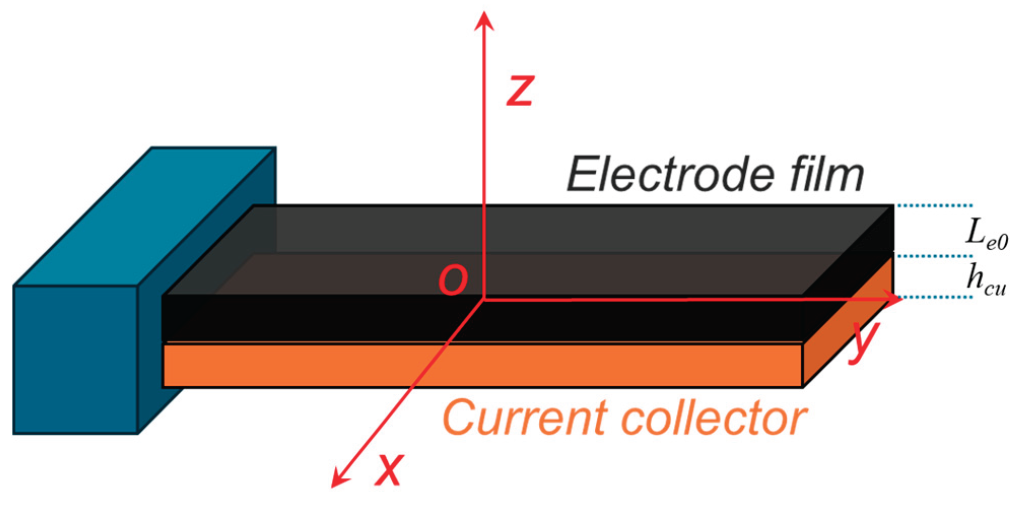
Disclaimer/Publisher’s Note: The statements, opinions and data contained in all publications are solely those of the individual author(s) and contributor(s) and not of MDPI and/or the editor(s). MDPI and/or the editor(s) disclaim responsibility for any injury to people or property resulting from any ideas, methods, instructions or products referred to in the content. |
© 2026 by the authors. Licensee MDPI, Basel, Switzerland. This article is an open access article distributed under the terms and conditions of the Creative Commons Attribution (CC BY) license (http://creativecommons.org/licenses/by/4.0/).
Copyright: This open access article is published under a Creative Commons CC BY 4.0 license, which permit the free download, distribution, and reuse, provided that the author and preprint are cited in any reuse.


