Submitted:
25 August 2025
Posted:
26 August 2025
You are already at the latest version
Abstract
Generalized Age-Period-Cohort (GAPC) models are mortality models incorporates stochasticity which can be represented in generalized linear or non-linear context. By fitting the data to either mortality model, one can make forecasts for the future under the extrapolation framework. Previous research indicates that the machine learning techniques can be applied to improve forecasting ability of such mortality models using different training/testing time periods. However, there is no consensus about generalizing this phenomenon on the improvement of fitted/forecasted mortality rates without depending on particular mortality model or models’ training/testing period. The idea in this study is to re-estimate the mortality rates obtained from each mortality models by applying tree-based machine learning methods within a procedure that creates suitable environment for integrating machine learning models for each GAPC models. This study shows that if the proper procedure is applied, the forecasting ability of each mortality model can be improved.
Keywords:
GAPC
; machine learning
; tree-based algorithms
; mortality forecasting
; stochastic mortality models
1. Introduction
Mortality rates form an important variable of actuarial calculations surrounding the valuation and pricing in life insurance. An actuary uses this parameter in modelling for annuity products where the resulting output is extremely delicate to this particular input. When building the models, stochastic processes are overlaid around the deterministic output to capture the range of expected lifetime uncertainty, and this hybrid output subsequently feeds into both internal economic-capital calculations and the capital frameworks prescribed by regulators [1]. It is crucial that under/over-estimated premiums may cause companies even bankrupt.
Forecasting mortality rates using mortality laws does not provide uncertainty regarding to the advances in mortality, since these models do not include any time component. Ultimately, the lack of an information on future mortality improvement may result in a faulty valuation of life insurance products. In addition, according to the Solvency II Framework Directive, a minimum amount of solvency capital should be maintained to prevent ruin [2]. The capital is associated with the risk of future mortality being significantly different to that implied by life expectancy and thus should be projected stochastically. Therefore, the necessity of stochastic mortality models to quantify the mechanism of mortality progress over the upcoming years and the uncertainty in the forecasts is crucial [3].
Making accurate forecasts of mortality pattern can inform not only demographers, but also researchers, governments and insurance companies about the future population size and longevity. Stochastic mortality modeling has become a pivotal area in current actuarial science and demography, offering valuable tools to predict mortality rates and to understand the complex trends and features behind human longevity. The ultimate goal of such models is to provide a more precise forecast of future mortality rates, for the purpose of allowing a better management of living more than expected of an individual. This exercise is crucial in the context of a number of applications, including the accurate pricing of insurance policies, construction plans of pension schemes, decision making of social security policies, and risk management in financial firms.
The Lee-Carter (LC) [4] model, presented by Ronald Lee and Lawrence Carter in 1992, can be considered as leading among them which has become a benchmark model in mortality forecasting. Together with the original model it’s extensions also have been used by academics, private sector practitioners and several statistics institutes for nearly three decades [5]. The LC model was earliest model taking the increased life expectancy trends into account which is related to the mortality improvement through time and has been used for forecasts of the United States social security system and federal budget [6,7]. In their paper [4], Lee and Carter introduced a stochastic method established on age-specific and time-varying components to capture and forecast the age specific death rates of the US population. Despite its simplicity, the LC model has demonstrated excellent results for fitting mortality for several countries.
Building on this work, several important extensions have been implemented to address Lee-Carter model’s limitations and enhance the predictive power. To handle the fundamental assumption of homoscedasticity of errors, Brouhns et al. [8] used LC model in an embedded Poisson regression framework. The Renshaw-Haberman (RH) [9] improved the LC model accuracy by capturing unique mortality experience influenced by the birth year (cohort) of individuals. Another model is the generalized form of the RH model that is so called age-period-cohort (APC) model, first introduced by Hobcraft et al. [10] and Osmond [11] which became visible in the demographic and actuarial literature by Currie [12]. A popular competitor of LC, a stochastic model to appear was the Cairns-Blake-Dowd (CBD) model [13]. Unlike the logarithmic transformation in the LC model, the CBD model applies a logit transformation to the probability of death, which is captured as linear or quadratic function of age which is also called M7 with an additional cohort effect [14]. Plat [15] combines LC and CBD models to explain the entire age range. The models mentioned above can be classified as Generalized-Age-Period-Cohort (GAPC) models that can be written in generalized linear/non-linear model (glm/gnm) setting [16]. In mortality modeling, glms/gnms are particularly useful for modeling mortality rates as a function of diverse explanatory variables such as age, sex, and cohort. Popular choices for the distribution of the outcome variable within glms include the binomial distribution for binary outcomes (e.g., survival vs. death) and the Poisson distribution for count data (e.g., number of deaths). The reason of choosing these mortality models is these models represent the vast majority of the stochastic mortality models together being a member of GAPC family [17,18]. For an extended overview, we refer Hunt and Blake [19], Haberman and Renshaw [20], Booth and Tickle [21], Pitacco et al. [22], Dowd et al. [23], Zamzuri and Hui [24] and Redzwan and Ramli [25]. The framework of GAPC model is detailly explained in the next section.
Recently, actuarial and demographic research have begun benefit from artificial intelligence, specifically machine learning. Humans and animals, learn from experience, that’s precisely what machine learning methods do, they copy that concept while teaching computers how to use historical data. These teaching methods are the algorithms those provide to learn the information from data which do not need any predetermined equations as a model [26]. Machine learning methods can be advantageous and learn from computations to make reliable and repeatable decisions and outcomes. It is a science not new, but newly invigorated. Stochastic mortality models, provide a parsimonious mechanism to capture systematic patterns in mortality through the scope of the features they contain. A prominent feature of age-period-cohort mortality models is the enforced smoothness and, as an extension, symmetry across age and over time to achieve model interpretability and tractability. However, mortuary dynamics in the real world are often asymmetrical in nature, based on heterogeneous shocks (i.e. pandemics, medical innovation, or region-specific health care reforms) and the nonlinear kinds of interactions that these models may not encapsulate [21]. Tree based machine learning techniques, represent an alternative approach since they are able to flexibly detect local deviations, non-monocities, and symmetry-breaking effects in mortality data [27].
To be able to model the mortality rates (i.e. age specific death rates) at population level which is a numeric outcome, age, period, cohort and gender can be used as features. When there is a response variable (mortality rate) and features as mentioned, the problem can be addressed as a regression which can be used to uncover the underlying pattern of mortality. When it comes to forecasting, mortality models can still produce poor forecasts of mortality rates while fitting almost perfect on training data. Previous research focused on improving mortality rates under this framework and obtained promising results. In addition to the traditional perspective, tree-based algorithms also can be used for regression. When the data has several attributes and the target value is numerical, then using tree-based algorithms for regression is suitable. From this point of view, in this study, supervised learning methods: decision trees (DC), random forest (RF), gradient boosting (GB) and extreme gradient boosting (XGB) which are all tree-based algorithms are used, to re-estimate the age-specific death rates obtained from the generalized age-period-cohort mortality models.
Machine learning has been increasingly used in major fields in science but the demography does not come first. Probably the main reason is researchers find it difficult to interpret the results since machine learning had been still believed as a “black box” [28]. This belief has come to end when Deprez et al. [29] showed that using mortality models can produce improved results together with the machine learning techniques. Deprez et. al. [29] used tree-based machine learning methods in a novel approach and encouraged researchers pondering more about machine learning along with demography. The work was based on improving the stochastic mortality model’s both fitting and forecasting ability by re-estimating the mortality rates using the features age, calendar year, gender and cohort with the help of machine learning techniques. Soon after, Levantesi and Pizzorusso [28] presented a new approach based on the same idea in Deprez et. al. [29] and used three mortality models to re-estimate the mortality rates obtained from the models. For forecasting the mortality rates, they treated the ratio of the observed and modeled number of deaths as mortality rates and used the same procedure of a mortality model. Staying within the context of improving mortality models’ accuracy using tree-based model, the research has gained momentum. Levantesi and Nigri [30] improved the Lee-Carter predictive accuracy by using random forest and p-splines methods. Bjerre [31] used tree-based methods to improve mortality rates using multi population data. Gyamerah et al. [32] developed a hybrid LC+ML (machine learning) model where the Lee–Carter time index is forecast using a stack of learners. Qiao et al. [33] applied a complex boosting/ensemble framework to long-term mortality. Across many countries, their method roughly halved the 20-year-forecast mean absolute percentage error compared to classic models. Finally, Levantesi et al. [34], used contrast trees as a diagnostic tool to identify the regions where the model gives higher error and used Friedman’s [35] boosting technique to improve the mortality model accuracy.
However, the research based on the idea of improving fitting and/or forecasting ability of a mortality model using machine learning techniques heavily depend on the pre-determined fitting and testing periods. Changing these periods mostly results in producing more errors than the original mortality model does. But then, focusing on the improving of fitting ability to rely on making better forecasts of mortality rates may not always a good idea especially when the historical mortality pattern that fitted to the model is not fully representative of the mortality pattern. The idea behind the out-of-sample tests helps solving this problem by determining model performance on unseen data with providing unbiased evaluation of how well the model can predict the future. From this point of view, in this study, we aimed to improve the forecasting ability of any mortality model using tree-based machine learning models by focusing on the out-of-sample testing. To be able to do it, we create a trade-off interval which allow the machine learning integrated model to give better forecasted mortality rates as an output without compromising the fitting quality of the re-estimated mortality rates over the fitting period at the same time. By doing so, using the procedure proposed in this study will enable to improve the mortality rates obtained from any mortality model. With this study, one can see the improved rates on the out-of-sample data without abandoning fitting period of the related mortality model.
The paper is organized as follows: in section 2, we briefly explain the GAPC models and the details of how to improve the forecasting ability of these mortality models. In the next section, we outline the four tree-based machine learning models in a regression setting. In section 4, we propose the procedure step by step and an application is illustrated. Finally, the discussion part is given.
2. Generalized Age-Period-Cohort Models
2.1. Data and Notation
The human mortality and population data at the population level often found in death counts and the exposure to risk (i.e. exposure) covering the ages and the calendar year shown as classical demographic and actuarial notation. The exposure to risk is measured by the person years lived, means that the contribution of an individual to the life line in terms of time. When the exposure is not available, the mid-year population is a good approximation. Stochastic mortality models transform the mortality rates by accounting at several combinations of the terms: age, period and cohort. These mortality rates are the observed series of either age specific death rates; or the probabilities of death; . However, the process underlying the mortality itself is continuous in nature, thus first, we need to make the transition from continuous state to the discrete one to be able to perform the mortality analysis. In a continuous state, the force of mortality shows the instantaneous death rate between t and dt where dt is really small. A single assumption of 0 ≤ s, u < 1, , implies the force of mortality remains constant over each age and calendar year. This assumption results in two important equation:
Let the number of deaths and the exposure to risk . Here is separated as (central exposed to risk) and (initial exposed to risk). which is also called central mortality rate can be easily calculated by dividing to the , while the which is also called initial mortality rate is calculated the same number of deaths divided by . When its absence, initial exposed to risk is approximated by adding the half of the death counts to the central exposed to risk. For practical purposes, the Figure 1 and Figure 2 below show the observed available mortality data for female population of Denmark.
The Figure 2, clearly represents the mortality rates reduction over years at almost each age. This phenomenon usually results in increasing life expectancy of the population over the years.
2.2. Age-Period-Cohort Structure
Generalized age-period-cohort model is a model capable of representing the response variable, a function of any mortality index, using linear or bilinear predictor structure of the features of age, period and cohort for a population [19]. GAPC models provide a powerful, flexible framework for mortality modeling by systematically incorporating these features effect. Their main advantage lies in significantly enhancing the reliability of parameter estimation and contributing to more robust mortality forecasting.
Hunt and Blake [19] discussed the vast majority of the stochastic mortality models are an expression of an age-period-cohort model. Currie [16] showed the form of generalized linear or non-linear model with the components:
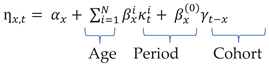
presents the link function of the response variable to the predictor structure. is the static age function, represents the general shape of mortality across the age range and fixed over the time period. is a set of age/period term where states the trend of mortality over time and denotes the pattern of mortality change across the ages. determines the effect of the cohorts through their lifetime and is the coefficient that modifies the [19].
If we treat the as random variables, the assumption can be made as: number of deaths follow either Poisson or Binomial distribution;
Then the link function is shown;
It is worth mentioning that there can be several link functions available, however it is convenient to use canonical link and pair the Poisson distributions with the log link function and the Binomial distributions with the logit link function (see, Villegas et al. [17], Currie [16], McCullagh and Nelder [37]).
The mortality models that can be expressed in glm/gnm form are available to be fitted to the data by using the StMoMo package in R [17,38]. In this study, tree-based algorithms are applied to each model included in the package StMoMo. These mortality models can be summarized into 3 groups: Lee-Carter [4] and its extensions, Cairns-Blake-Dowd (CBD) [13] and its extensions and Plat model [15] which is a hybridized version of classical age-period-cohort [12], LC [4] and CBD [13]. Table 1, shows the formal structure of the stochastic mortality models included in StMoMo.
Since CBD and M7 models’ response variable is , the transformation is done to using the equation 2. In addition to that, forecasting of mortality rates using mortality models is done using “auto.arima” function in R which selects the best Autoregressive Integrated Moving Averages (ARIMA) process of each index.
3. Tree-Based Machine Learning Models
Tree-based models have long been known as fundamental and successful class of machine learning algorithms. These models make predictions by applying a hierarchical, tree structure to the observations that is a unique take on solving problems whether they are classification (predicting categorical values) or regression (predicting numerical values). When it comes to prediction using tree-based methodologies, one basically generates a sequence of if-then rules from an initial root node (at the top) through a sequence of internal decision nodes and finalize in a terminal leaf node. To build this tree-like structure, a set of splitting rules are applied to divide the feature space into smaller groups until the stopping criteria is met. Stopping criteria is based on adjusting the hyperparameters which are non-learnable parameters (i.e. maximum depth of a tree, minimum samples in a node, etc.) that are defined prior to the commencement of the learning process. They serve to control various aspects of the learning algorithm and can significantly influence the model's performance and behavior. The careful tuning of these hyperparameters is paramount for achieving improved model performance and, critically, for mitigating the risk of overfitting.
Tree-based models are non-parametric supervised learning algorithms, known as being incredibly flexible for a variety of predictive tasks. These models' innate ability to capture complex patterns and non-linear interactions in complex datasets is a major advantage over conventional linear models. They are especially effective in real-world applications where relationships between variables are rarely purely linear, in contrast to linear models, which presume a direct, linear relationship between features and outcomes. This ability is useful to use when the mortality itself is considered a non-linear process.
In this study we used four popular types of tree-based algorithms which is believed to reflect the majority of the methods shows a tree structure and we can briefly classify them as [39]:
- Decision tree model, the substructure of tree-based models,
- Random forest model, “ensemble” method constructs more than one decision tree,
- Gradient boosting model, “ensemble” method constructs decision trees sequentially,
- Extreme gradient boosting model, “ensemble” method constructs decision trees in parallel.
In this study, since the response variable is continuous, the tree-based methods are studied in a regression framework.
3.1. Decision Trees
Decision Trees (DT), first introduced by Brieman et al. [40], serve as the foundational element for all tree-based models. Understanding their specific application in regression provides crucial context for the more complex ensemble methods.
To build a decision tree, an information must be defined for splitting the data. For discrete variables, popular choices would be the Gini information or entropy, however when the response variable is continuous, an error-based information is needed. Let S represents total squared errors of the tree T, [41] showed that;
Final prediction is;
The splitting process is stopped by minimizing S with predefined hyperparameters, and the final predictions in each leaf are obtained.
3.2. Random Forest
In 2001, Breiman [42] introduced a powerful tree-based algorithm called Random Forest (RF). In random forest, a bootstrap sample of the data, or n observations chosen with replacement from the initial n rows, is used to calculate each tree. This method is known as "bagging" which is derived from "bootstrap aggregating" [43]. Predictions are found by pooling the predictions of all trees, means majority voting for classification problems and averaging of the predictions from all trees for regression problems.
The progression from single decision trees to ensemble methods like random forests is more than an incremental improvement in accuracy; it represents a fundamental shift in how the bias-variance trade-off is addressed. Single decision trees, by their nature, tend to be high-variance, low-bias models, meaning they can fit the training data very closely but are sensitive to small variations in that data, leading to poor generalization. Bagging, as implemented in random forests, primarily reduces variance by averaging the predictions of multiple independently trained trees, thereby mitigating the overfitting tendency of individual trees.
Final predictions are simply the averages of each prediction of the individual trees.
3.3. Gradient Boosting
Gradient Boosting (GB) algorithm makes accurate predictions with the combination of many decision trees in a single model. It is an algorithmic predictive modeling invented by Friedman [44], that learns from errors to build up predictive strength. Unlike random forest, gradient boosting combines several weak models of prediction into a single ensemble to improve accuracy. Typically, gradient boosting uses decision trees, in an ensemble and are trained sequentially with the idea of minimizing errors [45].
The algorithm fits a decision tree to the residuals of initial model. In this instance “fitting a tree based on the current residuals” means that we are fitting a tree, with the residuals as response values rather than the original outcome. This fitted tree now becomes a part of the fitted function and the residuals are updated. By doing so, f is being improved bit by bit in the regions in which is not performing good. The shrinkage parameter λ also slows down the process, leading to more and differently shaped trees applied to the residuals. In general, slow learners lead to a better overall performance [46,47].
Final predictions are shown as;
where is learning rate, M represents total number of trees, stands for m. regression tree output. Each is trained on the residuals that is shown as;
where L is the loss function aimed to minimize.
3.4. Extreme Gradient Boosting
Extreme gradient boosting (XGB) method developed by Chen and Guestrin [48], is an improved implementation of GB basically with the same framework that combines weak learner trees into strong learning by adjusting the residuals. Unlike gradient boosting method, the trees grown in parallel, not sequentially. Also, extreme gradient boosting method has built-in regularization to prevent overfitting by penalizing model complexity.
Final predictions are estimated similarly but with a more regularized objective function [49];
with trying to the minimize the function:
4. ML Integrated Model Development
4.1. Improving the Accuracy of a GAPC Model
The idea on improving mortality models’ accuracy based on approximating the mortality rates of the final model to the observed ones. If the total error, which is the difference between modeled and observed rates, is reduced, then the proposed model would have improved the original mortality model.
In practice, first the data is fit to each mortality model. Then the number of deaths at age x and year t is able to be extracted from the model (). Here, “mdl” indicates the mortality model in use. Similarly, when of the model is re-estimated using machine learning methods, then the mortality rate is written as . According to the Deprez et. al. [29] and Levantesi and Pizzorusso [28], improved mortality rates can be estimated as:
Here is a ratio between the estimated and the observed death counts. Consider a coefficient that can be multiplied with the number of deaths and rewrite the equation;
With a perfect model, the coefficient would be equal to 1. However, in the real world, there is no model that fits perfectly to any mortality data. Even, that model exists, it would be useless for forecasting since it lacks of generalizing the mortality pattern and overfits the presented data. Therefore, the idea behind improving the accuracy of a mortality model is to calibrate the coefficient by applying the tree-based algorithms under a regression framework with given features. We can illustrate the model as follow;
Here, the = is found as a solution of the equation above by using four types of tree-based algorithms. After estimating for each age and year using the machine learning algorithms, it is applied to the mortality rates obtained from the GAPC models to get the improved mortality rates.
4.2. Evaluating the Forecasting Performance of a Model
While practicing the machine learning techniques, data is split into train and test parts to make a particular model being fit to the data and see how it performs on the data. In-sample test use the same data for evaluating the model and measure how well it fits. However, this type of test lack of generalizing and accommodates risk of overfitting. Out-of-sample test on the other hand, do not use a part of the data in the training process. In addition to these kinds of tests, hold-out test is a type of out-of-sample test which uses separate unseen data used only once at the end for understanding the performance of the model which is reasonably unbiased estimate.
The practice in this study is a combination of out-of-sample tests qualifying the forecasting accuracy on unseen data. But the forecasting evaluation is based on mortality rates which is not used in machine learning process. is the only variable calibrated in a regression framework with tree-based methods and multiplied with the mortality rates of the mortality models. These results are then compared with the observed mortality rates. While k-fold cross-validation is used for calibration of , hold-out test is used for qualifying the forecasting accuracy of tree-based integrated model.
To assess the goodness of fit and forecast of the GAPC and the tree-based improved models, Root Mean Squared Error (RMSE) is used. RMSE is extensively exercised in regression problems as a loss function and in model evaluation, because of its very intuitive interpretation. The RMSE is calculated as follows;
where are predicted, are observed and is the number of observations.
5. A Procedure for Improving the Forecasting Ability
The procedure means applying all methods sequentially to get the results without the need of human interaction. Briefly; after fitting a GAPC model to the data and obtain the mortality rates, is calculated. Then mortality model specific is estimated using tree-based model for both training and hold-out testing period with all possible set of hyperparameters. By multiplying the forecasted (estimated over the hold-out testing period) with which is the mortality rates forecasted using mortality model, machine learning integrated mortality rates () can easily be estimated. After that, for each hyperparameter set, the RMSE of ML integrated mortality rates against observed ones are calculated and lower than the RMSE of mortality models are chosen. For eliminating the randomness of the success of this process, the set of hyperparameters use to calibrate the and give the lower RMSE on the testing period, are checked if they give lower RMSE on the training period as well. Thus, a trade-off interval is created for lowering the error of original mortality model on both periods. The step-by-step explanation and the graphical representation are given below.
The Procedure
- 1.
- Reserve a hold-out testing period,
- 2.
- Fit a mortality model to the training data,
- 3.
- Extract fitted mortality rates,
- 4.
- Calculate for each age and year,
- 5.
- Forecast with same mortality model over the testing period,
- 6.
- Extract forecasted mortality rates and calculate model RMSE,
- 7.
- Calibrate with tree-based methods;
- a.
- Determine lower & upper limits of hyperparameters,
- b.
- Extract re-estimated series calculated with different set of hyperparameters,
- 8.
- Obtain each series using tree-based methods,
- 9.
- Calculate each series of over the testing period,
- 10.
- Identify the series that give less RMSE for testing period,
- 11.
- Find series used to forecast and calculate over training period,
- 12.
- Search for series that also give less RMSE for training period,
- 13.
- Repeat the steps for each mortality model.
By following through the steps, series of improved mortality rates for both training and testing periods will be estimated. Under these circumstances, machine learning techniques can improve the mortality models’ forecasting accuracy without relying on the fixed fitting or testing period. At the end, researcher can make robust and reliable forecasts about future mortality.
The Figure 3, represents the steps in a clear way, make the whole procedure more visible. Additionally, it is important to remember that these values are based on mortality rates either calculated by mortality models or those multiplied with the psi which is calibrated with tree-based models. Mortality rates themselves are not subject to any machine learning process. With the help of this flexible approach, researcher can adjust training and testing period of the preferred mortality model and make improved forecast of future mortality.
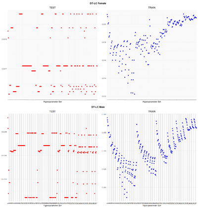
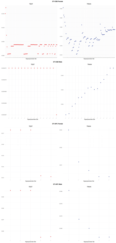
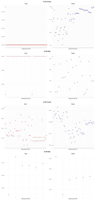
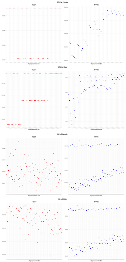
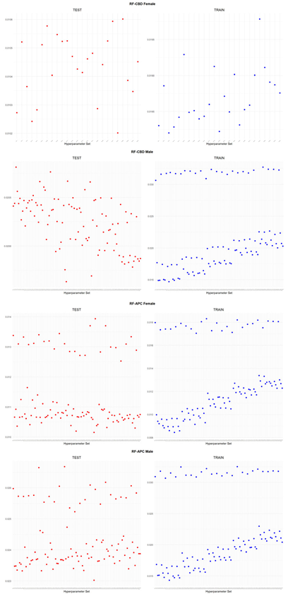
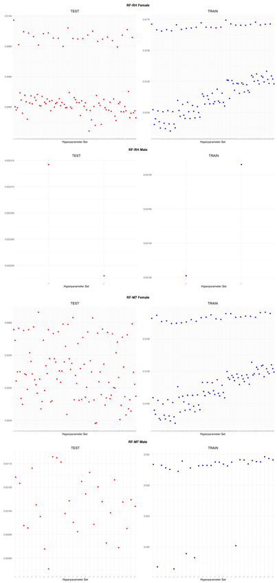
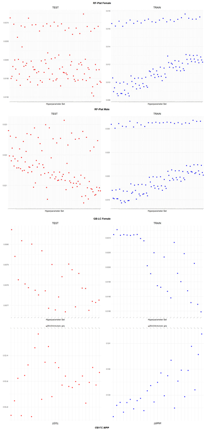
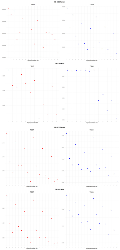
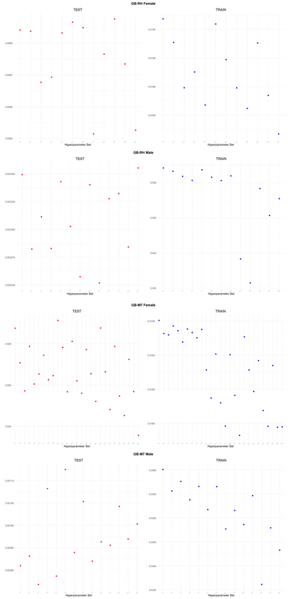
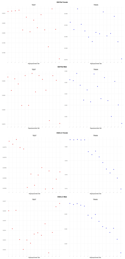
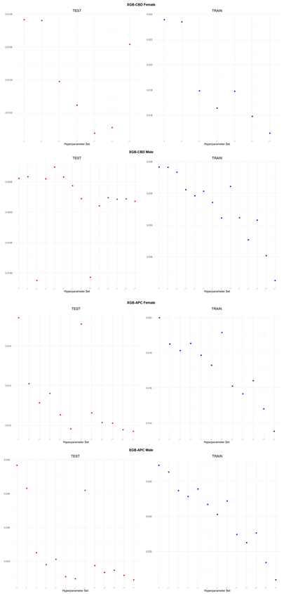
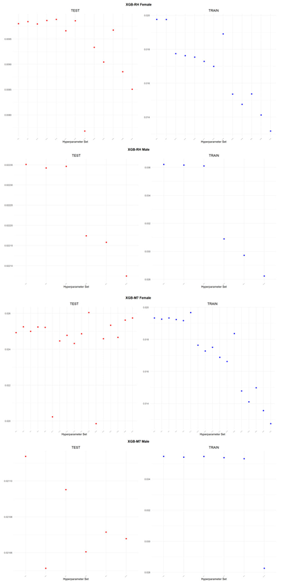
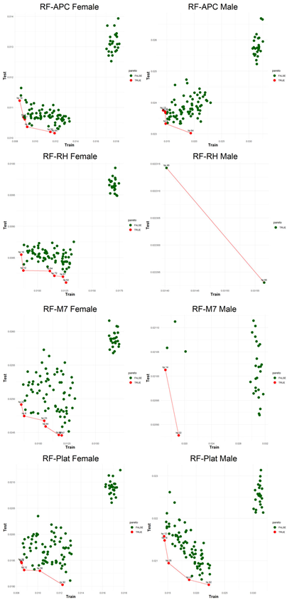
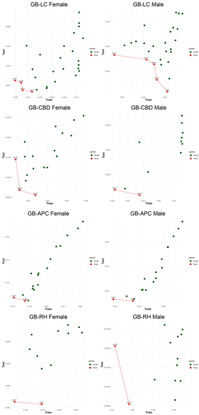
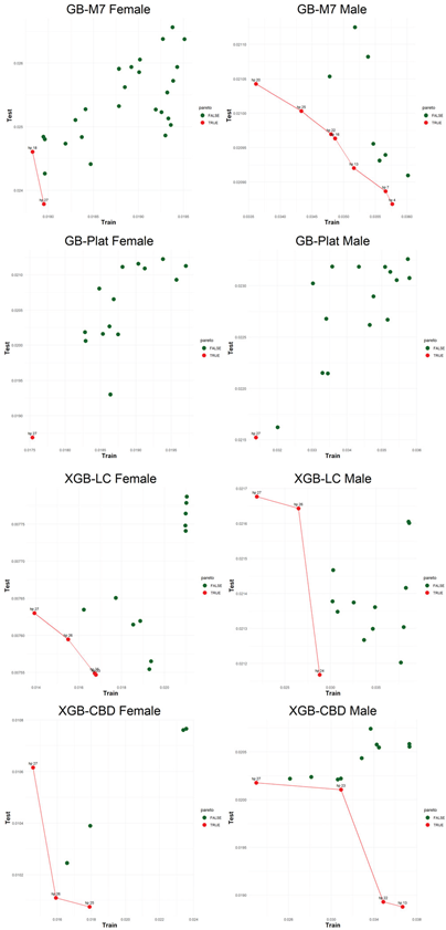
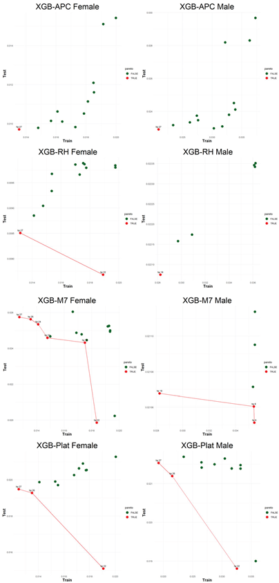
An application is performed for practical representation; the Figure 4, shows only ML integrated model RMSEs by hyperparameter set that is less than pure mortality model’s RMSEs for both periods (figures of the other models are presented in the Appendix A.1.). The procedure finds lower error for testing period first, then obtains the lower errors for training period using same hyperparameter sets against the pure mortality model. As can be seen from the Figure 4, the hyperparameter set that gives the lowest error during the test period may not always be the hyperparameter set that gives the lowest error during the training period. In fact, it may even produce higher errors than the pure mortality model. Therefore, while focusing on achieving lowest error during the testing period, it is also necessary to find the set of hyperparameters that gives lower error than the pure mortality model over the training period.
Table 2, shows minimum values of RMSE over the testing and training period for pure mortality models and ML integrated models (male version of the table 2 is given in the Appendix B.1.). The same data set used as for creating the Figure 4. As it can seen from the table, including all ML integrated methods, using the same hyperparameter set that works best for testing period may produce higher error for the training period while different hyperparameter set give less error over the training period. At the same time, the error should not be higher than the pure mortality model’s error. Although, the users notice this trade-off mechanism, choosing the best combination still be confusing. Hence, we use Pareto [51] optimal method to find the dominant combination of hyperparameter set. In many instances it is said there are conflicting objective functions and that there exist Pareto optimal solutions. A susceptible solution is said to be nondominated if none of the objective functions can take on a new value to improve its value without deteriorating some of the other objective functions. These solutions are referred to as Pareto optimal. When no other preference information is supplied, all Pareto optimal solutions are said to be equally good [52]. In this regard, efficient frontier is constructed which shows the Pareto optimal values and connect them together.
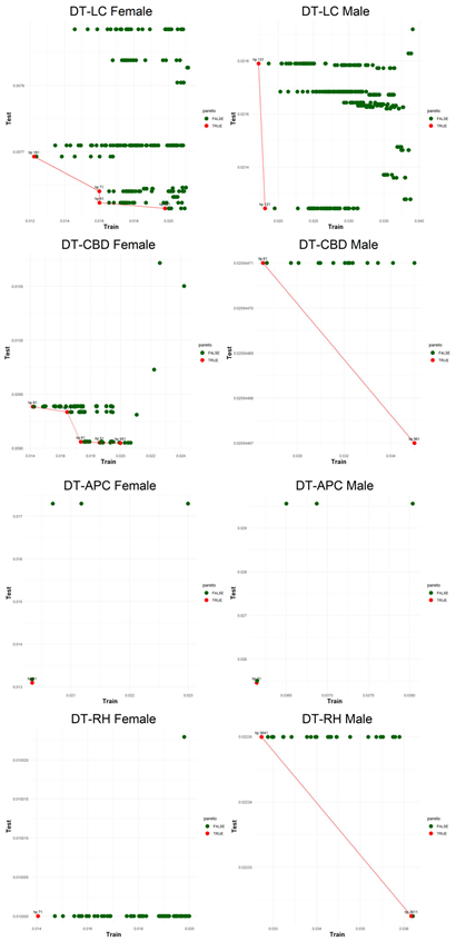
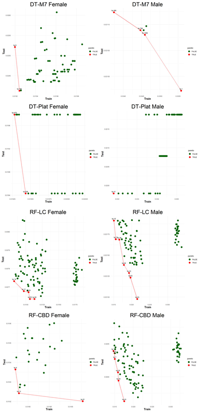
Figure 5, visualizes the Pareto optimal values of the hyperparameter set that gives lower error over both training and testing periods (figures of the other models are presented in the Appendix B.2.). The efficient frontier concept guides users in choosing the best balance of test and train errors.
6. Discussion
Mortality forecasting does not have a long history in the demographic or actuarial literature. Starting with Lee and Carter [4], mortality forecasting has been gaining momentum, with comprehensive studies being conducted frequently. In recent years, researchers have focused their attention on integrating advanced statistical methods into their studies related to the length of human life. These studies show that when this growing interest is combined with demographic models, more robust and consistent results emerge.
Data for each population has its own unique characteristics. Mortality models aim to explain the mortality pattern and make accurate forecasts based on the historical data. In this context, machine learning can help understand the non-linear nature of the mortality rates, which generally tend to decline at almost every age each year. Declining pattern of mortality rates that results in increasing life expectancy pose a significant risk to the sustainability of social security, elderly care and pension systems which implies that we need more precise and robust forecasts of mortality.
This study presents a general procedure for improving the forecasting accuracy of mortality models using most common tree-based machine learning methods, by creating a flexible environment on the train/test data which is critical for measuring the goodness of fit/forecasting. This will enable researchers to choose the most suitable mortality model for population-specific mortality data and perform best practices of forecasts for the future mortality.
This study focuses on facilitating the integration of mortality models into machine learning methods within a general framework and to demonstrate that forecasting accuracy can be improved under specified conditions, rather than taking advantage of analyzing specific periods that increase forecasting accuracy. This study guides researchers in the right direction by offering a flexible structure while choosing the test data, which is one of the most important factors in measuring the quality of the model when using mortality models. We believe, researchers will enable to make more accurate forecasts for the future.
Author Contributions
Conceptualization, Ö.B. and M.B.; methodology, Ö.B.; software, Ö.B.; formal analysis, Ö.B.; writing—original draft preparation, Ö.B.; writing—review and editing, Ö.B. and M.B; visualization, Ö.B.; supervision, M.B. All authors have read and agreed to the published version of the manuscript.
Funding
This research received no funding.
Data Availability Statement
Mortality data can be downloaded free of charge from the website: www.mortality.org.
Acknowledgments
This study is prepared as a part of PhD. project of Özer Bakar under the supervision of Murat Büyükyazıcı, conducted in Hacettepe University, Institute of Science, Türkiye.
Conflicts of Interest
The authors declare no conflict of interest.
Appendix A
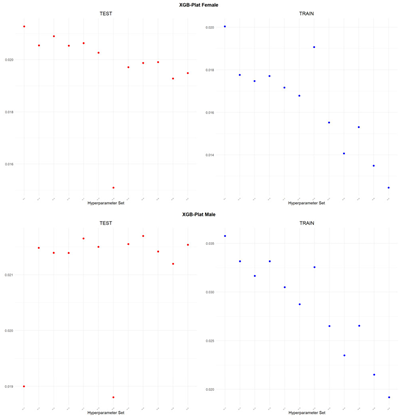
Appendix A.1. Test and Train RMSE of ML Integrated Models Below Pure Mortality Model’s RMSE in Use
The appendix A.1 includes figures of RMSE values lower than the pure mortality model in use for both periods. Data: The ages 65-99 and the years 1960-2010 for training and 2011-2020 for testing (hold-out) periods, female and male population of Denmark.
Appendix A.2. Hyperparameter Set and Limits for Each ML Model
Below, hyperparameters limits are presented. The algorithm uses each combination within the limits and estimates series.

Table 3.
Hyperparameter set of each model.
| Decision Tree | Random Forest | Gradient Boosting | Extreme Gradient Boosting | |||||||
|---|---|---|---|---|---|---|---|---|---|---|
| LC, RH | CBD | APC | M7, Plat | All | All | All | ||||
| cp | 0.001 | 0.001 | 0.01 | 0.001 | mtry | 1:4 | shrinkage | 0.01, 0.05, 0.1 | nrounds | 50, 100, 150 |
| minsplit | 1:10 | 1:10 | 1:10 | 1:5 | num.trees | 50,100,150,200,300 | n.trees | 50, 100, 150 | eta | 0.01, 0.05, 0.1 |
| maxdepth | 1:30 | 1:10 | 1:10 | 1:30 | min.node.size | 1:5 | interaction.depth | 1, 3, 5 | max_depth | 1, 3, 5 |
| minbucket | 1:20 | 1:10 | 1:10 | 10:40 | ||||||
Appendix B.1. Efficient Frontier of the Models
Appendix B.2. Male Version of Table 2.
Table 4.
Minimum RMSE value of the testing period with corresponding RMSE of the training period and minimum RMSE value of the training period*. Data: Denmark male population, years between 1960:2010 (train), 2011:2020 (test), ages between 65:99. .
Table 4.
Minimum RMSE value of the testing period with corresponding RMSE of the training period and minimum RMSE value of the training period*. Data: Denmark male population, years between 1960:2010 (train), 2011:2020 (test), ages between 65:99. .
| Pure | DT | RF | GB | XGB | ||||||||||
|---|---|---|---|---|---|---|---|---|---|---|---|---|---|---|
| Test | Train | Min Test | Train | Min Train |
Min Test | Train | Min Train |
Min Test | Train | Min Train |
Min Test | Train | Min Train |
|
| LC | 2.1922 | 4.0438 | 2.1244 | 1.8127 | 1.7225 | 2.0977 | 2.1543 | 1.5052 | 2.1233 | 3.8256 | 3.3274 | 2.1167 | 2.8815 | 2.1907 |
| CBD | 2.0877 | 3.7642 | 2.0545 | 3.5016 | 2.8520 | 1.9631 | 1.7566 | 1.4695 | 2.0233 | 3.4770 | 3.3159 | 1.8876 | 3.6668 | 2.2994 |
| APC | 2.9781 | 3.9230 | 2.5461 | 3.6140 | 3.6140 | 2.3023 | 1.9350 | 1.4311 | 2.3170 | 3.3490 | 3.1862 | 2.2897 | 2.0956 | 2.0956 |
| RH | 2.2360 | 3.6468 | 2.2323 | 3.6204 | 3.2732 | 2.2293 | 3.1565 | 3.1402 | 2.2252 | 3.3834 | 3.3150 | 2.2074 | 2.8230 | 2.8230 |
| M7 | 2.1140 | 3.6614 | 2.0973 | 3.5582 | 3.3742 | 2.0878 | 1.9122 | 1.7146 | 2.0868 | 3.5766 | 3.3615 | 2.1051 | 3.5421 | 2.8256 |
| Plat | 2.3274 | 3.6173 | 1.9786 | 3.2534 | 3.1819 | 2.0428 | 2.2212 | 1.4345 | 2.1522 | 3.1389 | 3.1389 | 1.8804 | 3.2549 | 1.9184 |
*: Results are multiplied with 102 to make them fit the table.
It is worth mentioning that these results are based on a single application carried out within a limited year and age range in the possible state-space for data of a specific country. Our application aimed to find the improved mortality rates using each tree-based algorithm in a reasonable short amount of time. Users should carefully select the train-test data and specifically determine the hyperparameter limits to avoid possible amount of time to obtain the results. Using additional hyperparameter and extending the limits of the hyperparameters can substantially increase the working time of the algorithms.
References
- Richman, R. AI in Actuarial Science - A Review of Recent Advances - Part 2. Ann. Actuar. Sci. 2021, 15, 230–258. [CrossRef]
- Commentary on Title IV of Directive 2009/138/EC on the Taking up and Pursuit of the Business of Insurance and Reinsurance (Solvency II); 2009.
- Cairns, A.J.G.; Blake, D.; Dowd, K. Modelling and Management of Mortality Risk: A Review. Scand. Actuar. J. 2008, 1238, 79–113. [CrossRef]
- Lee, R.D.; Carter, L.R. Modeling and Forecasting U. S. Mortality. J. Am. Stat. Assoc. 1992, 87, 659. [CrossRef]
- Basellini, U.; Camarda, C.G.; Booth, H. Thirty Years on: A Review of the Lee–Carter Method for Forecasting Mortality. Int. J. Forecast. 2023, 39, 1033–1049. [CrossRef]
- Zeddouk, F.; Devolder, P. Mean Reversion in Stochastic Mortality: Why and How? Eur. Actuar. J. 2020, 10, 499–525. [CrossRef]
- Long-Term Budgetary Pressures and Policy Options; Washington, D.C., 1998.
- Brouhns, N.; Denuit, M.; Vermunt, J.K. A Poisson Log-Bilinear Regression Approach to the Construction of Projected Lifetables. Insur. Math. Econ. 2002, 31, 373–393. [CrossRef]
- Renshaw, A.E.; Haberman, S. A Cohort-Based Extension to the Lee-Carter Model for Mortality Reduction Factors. Insur. Math. Econ. 2006, 38, 556–570. [CrossRef]
- Hobcraft, J.; Menken, J.; Preston, S. Age, Period, and Cohort Effects in Demography: A Review. Popul. Index 1982, 48, 4–43. [CrossRef]
- Osmond, C. Using Age, Period and Cohort Models to Estimate Future Mortality Rates. Int. J. Epidemiol. 1985, 14.
- Currie, I.D. Smoothing and Forecasting Mortality Rates with P-Splines. 2006.
- Cairns, A.J.G.; Blake, D.; Dowd, K. A Two-Factor Model for Stochastic Mortality with Parameter Uncertainty: Theory and Calibration. J. Risk Insur. 2006, 73, 687–718. [CrossRef]
- Cairns, A.J.G.; Blake, D.; Dowd, K.; Coughlan, G.D.; Epstein, D.; Ong, A.; Balevich, I. A Quantitative Comparison of Stochastic Mortality Models Using Data From England and Wales and the United States. North Am. Actuar. J. 2009, 13, 1–35. [CrossRef]
- Plat, R. On Stochastic Mortality Modeling. Insur. Math. Econ. 2009, 45, 393–404. [CrossRef]
- Currie, I.D. On Fitting Generalized Linear and Non-Linear Models of Mortality. Scand. Actuar. J. 2016, 2016, 356–383. [CrossRef]
- Villegas, A.M.; Millossovich, P.; Kaishev, V.K. StMoMo: Stochastic Mortality Modeling in R. J. Stat. Softw. 2018, 84. [CrossRef]
- Hunt, A.; Blake, D. A General Procedure for Constructing Mortality Models. North Am. Actuar. J. 2014, 18, 116–138. [CrossRef]
- Hunt, A.; Blake, D. On the Structure and Classification of Mortality Models. North Am. Actuar. J. 2021, 25, S215–S234. [CrossRef]
- Haberman, S.; Renshaw, A. A Comparative Study of Parametric Mortality Projection Models. Insur. Math. Econ. 2011, 48, 35–55. [CrossRef]
- Booth, H.; Tickle, L. MORTALITY MODELLING AND FORECASTING: A REVIEW OF METHODS By H. Booth and L. Tickle. Ann. Actuar. Sci. H., L. Tickle, ‘MORTALITY Model. Forecast. A Rev. METHODS By H. Booth L. Tickle’, Ann. Actuar. Sci. 3/I/II (2008), 3–43 <https//openresearch-repository.anu.edu.au/bitstream/1885/55237/2/ 2008, 3, 3–43.
- Pitacco, E., Denuit, M., Haberman, S., Olivieri, A. Modelling Longevity Dynamics for Pensions and Annuity Business; Oxford University Press: Okford, 2009.
- Dowd, K.; Cairns, A.J.G.; Blake, D.; Coughlan, G.D.; Epstein, D.; Khalaf-Allah, M. Evaluating the Goodness of Fit of Stochastic Mortality Models. Insur. Math. Econ. 2010, 47, 255–265. [CrossRef]
- Zamzuri, Z.H.; Hui, G.J. Comparing and Forecasting Using Stochastic Mortality Models: A Monte Carlo Simulation. Sains Malaysiana 2020, 49, 2013–2022. [CrossRef]
- Redzwan, N.; Ramli, R. A Bibliometric Analysis of Research on Stochastic Mortality Modelling and Forecasting. Risks 2022, 10. [CrossRef]
- Nithya C; Saravanan V A Study of Machine Learning Techniques in Data Mining. Int. Sci. Ref. Res. J. © 2018 SISRRJ | 2018, 1, 31–34.
- Richman, R.; Wüthrich, M. V. A Neural Network Extension of the Lee-Carter Model to Multiple Populations. Ann. Actuar. Sci. 2021, 15, 346–366. [CrossRef]
- Levantesi, S.; Pizzorusso, V. Application of Machine Learning to Mortality Modeling and Forecasting. Risks 2019, 7, 1–19. [CrossRef]
- Deprez, P.; Shevchenko, P. V.; Wüthrich, M. V. Machine Learning Techniques for Mortality Modeling. Eur. Actuar. J. 2017, 7, 337–352. [CrossRef]
- Levantesi, S.; Nigri, A. A Random Forest Algorithm to Improve the Lee–Carter Mortality Forecasting: Impact on q-Forward. Soft Comput. 2020, 24, 8553–8567. [CrossRef]
- Bjerre, D.S. Tree-Based Machine Learning Methods for Modeling and Forecasting Mortality. ASTIN Bull. 2022, 52, 765–787. [CrossRef]
- Gyamerah, S.A.; Mensah, A.A.; Asare, C.; Dzupire, N. Improving Mortality Forecasting Using a Hybrid of Lee–Carter and Stacking Ensemble Model. Bull. Natl. Res. Cent. 2023, 47. [CrossRef]
- Qiao, Y.; Wang, C.W.; Zhu, W. Machine Learning in Long-Term Mortality Forecasting. Geneva Pap. Risk Insur. Issues Pract. 2024, 49, 340–362. [CrossRef]
- Levantesi, S.; Lizzi, M.; Nigri, A. Enhancing Diagnostic of Stochastic Mortality Models Leveraging Contrast Trees: An Application on Italian Data. Qual. Quant. 2024, 58, 1565–1581. [CrossRef]
- Friedman, J.H. Contrast Trees and Distribution Boosting. Proc. Natl. Acad. Sci. U. S. A. 2020, 117, 21175–21184. [CrossRef]
- Human Mortality Database Available online: www.mortality.org.
- McCullagh P., N.J.A. Generalized Linear Models; 2nd ed.; Chapman and Hall: London, 1989; ISBN 9780128186299.
- RStudio: Integrated Development for R. 2020.
- Gross, K. Tree-Based Models: How They Work in Plain English Available online: https://blog.dataiku.com/tree-based-models-how-they-work-in-plain-english.
- Breiman, L., Friedman, J. H., Olshen, R. A., Stone, C.J. Classification and Regression Trees; Boca Raton: CRC Press, 1984.
- Shalizi, C. Regression Trees; 2006.
- Breiman, L. Random Forests. Mach. Learn. 2001, 45, 32.
- Theobald, O. Machine Learning for Absolute Beginners; 2017; ISBN 1549617214.
- Friedman, J.H. Greedy Function Approximation: A Gradient Boosting Machine. Ann. Stat. 2001, 29, 1189–1232.
- Gradient-Boosting @ Www.Ibm.Com Available online: https://www.ibm.com/think/topics/gradient-boosting.
- Truong, H.P. Predicting Aircraft Availability: A Machine Learning Approach, California State University, 2022.
- James, G.; Witten, D.; Hastie, T.; Tibshirani, R. An Introduction to Statistical Learning; Springer Texts in Statistics, 2023; ISBN 9780387781884.
- Chen, T.; Guestrin, C. XGBoost: A Scalable Tree Boosting System. Proc. ACM SIGKDD Int. Conf. Knowl. Discov. Data Min. 2016, 13-17-Augu, 785–794. [CrossRef]
- Sheridan, R.P.; Wang, W.M.; Liaw, A.; Ma, J.; Gifford, E.M. Extreme Gradient Boosting as a Method for Quantitative Structure-Activity Relationships. J. Chem. Inf. Model. 2016, 56, 2353–2360. [CrossRef]
- Bhuse, P.; Gandhi, A.; Meswani, P.; Muni, R.; Katre, N. Machine Learning Based Telecom-Customer Churn Prediction. Proc. 3rd Int. Conf. Intell. Sustain. Syst. ICISS 2020 2020, 1297–1301. [CrossRef]
- Pareto, V. Cours d’Économie Politique. In; 1986; Vol. 1.
- Chang, K.-H. Multiobjective Optimization and Advanced Topics; 2015; ISBN 9780123820389.
Figure 1.
Death counts (left) and exposure to risk (right) by ages for female population of Denmark in 2024. Source: Authors own elaborations using Human Mortality Database [36].
Figure 1.
Death counts (left) and exposure to risk (right) by ages for female population of Denmark in 2024. Source: Authors own elaborations using Human Mortality Database [36].
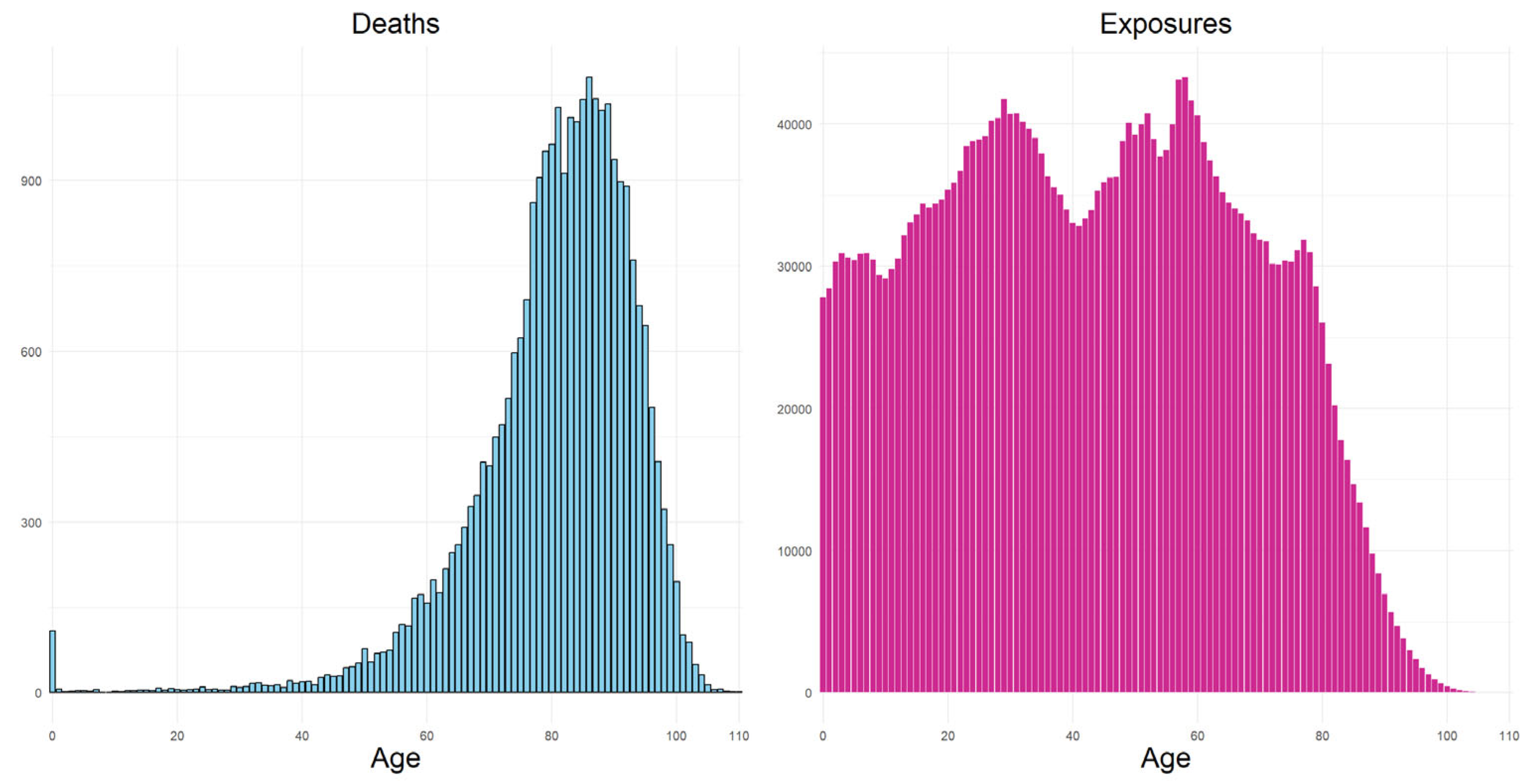
Figure 2.
Evolution of age specific death rates on scale between the years 1950-2024 for female population of Denmark. Source: Authors own elaborations using Human Mortality Database [36].
Figure 2.
Evolution of age specific death rates on scale between the years 1950-2024 for female population of Denmark. Source: Authors own elaborations using Human Mortality Database [36].
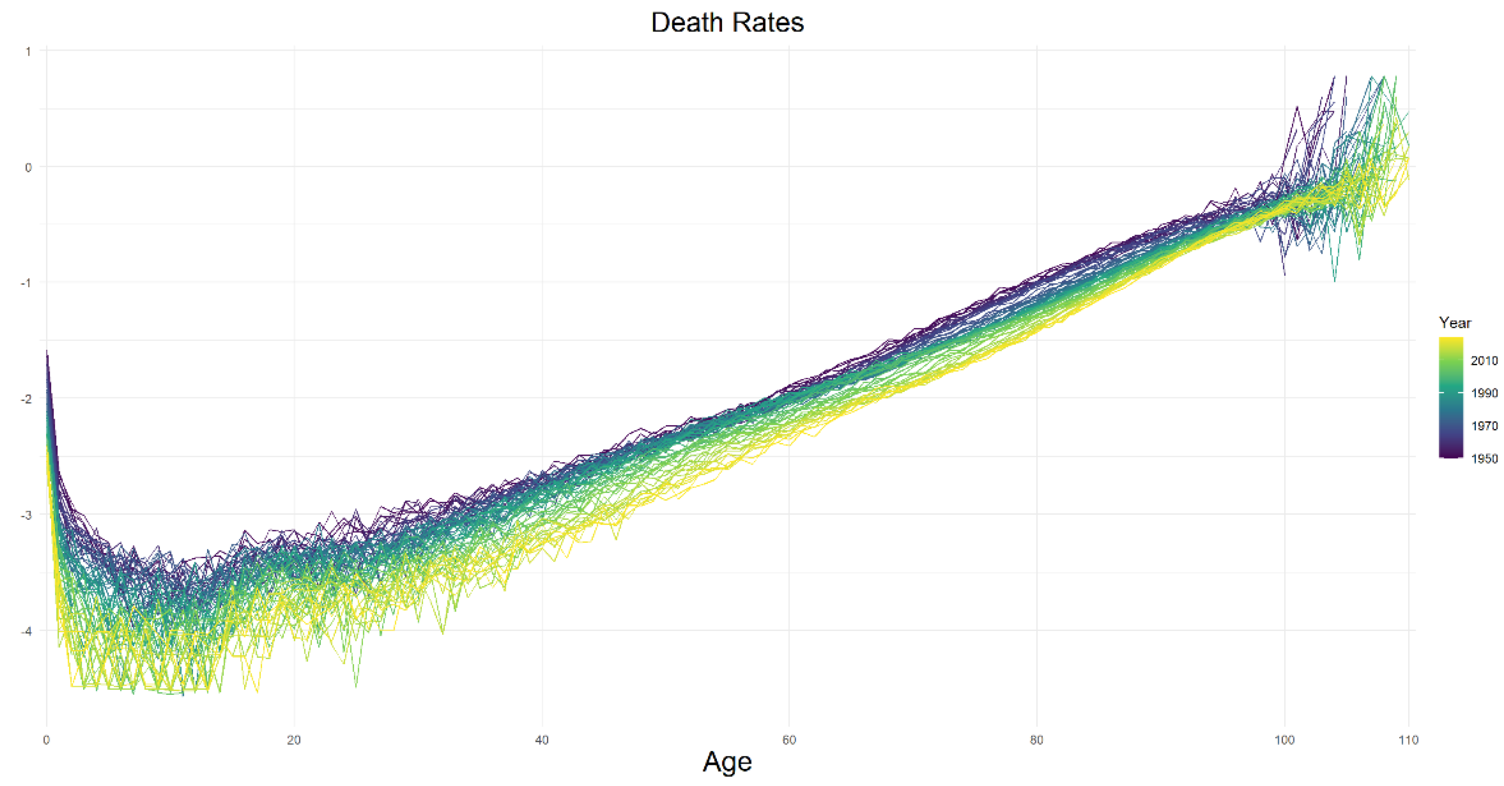
Figure 3.
Graphical illustration of the procedure. Source: Created by the authors using Canva. Calculations on the left side of the graph are based on training period while those on the right side are based on testing period. RMSE values are calculated against observed values of mortality rates. At the end, steps should be repeated for the other mortality models and results should be compared.
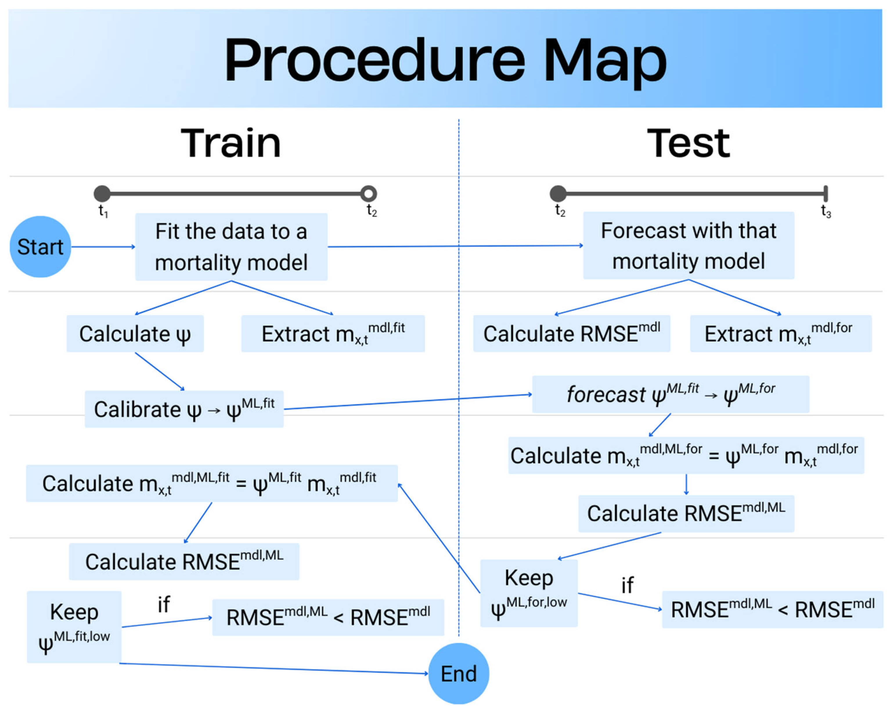
Figure 4.
RMSE values lower than the pure mortality model. Data: The ages 65-99 and the years 1960-2010 for training and 2011-2020 for testing (hold-out) periods, female population of Denmark. Model: RF integrated CBD model (hyperparameters and their limits are given in the Appendix A.2.). The RMSE of the CBD model is 0.010778 for test and 0.026751 for training period.
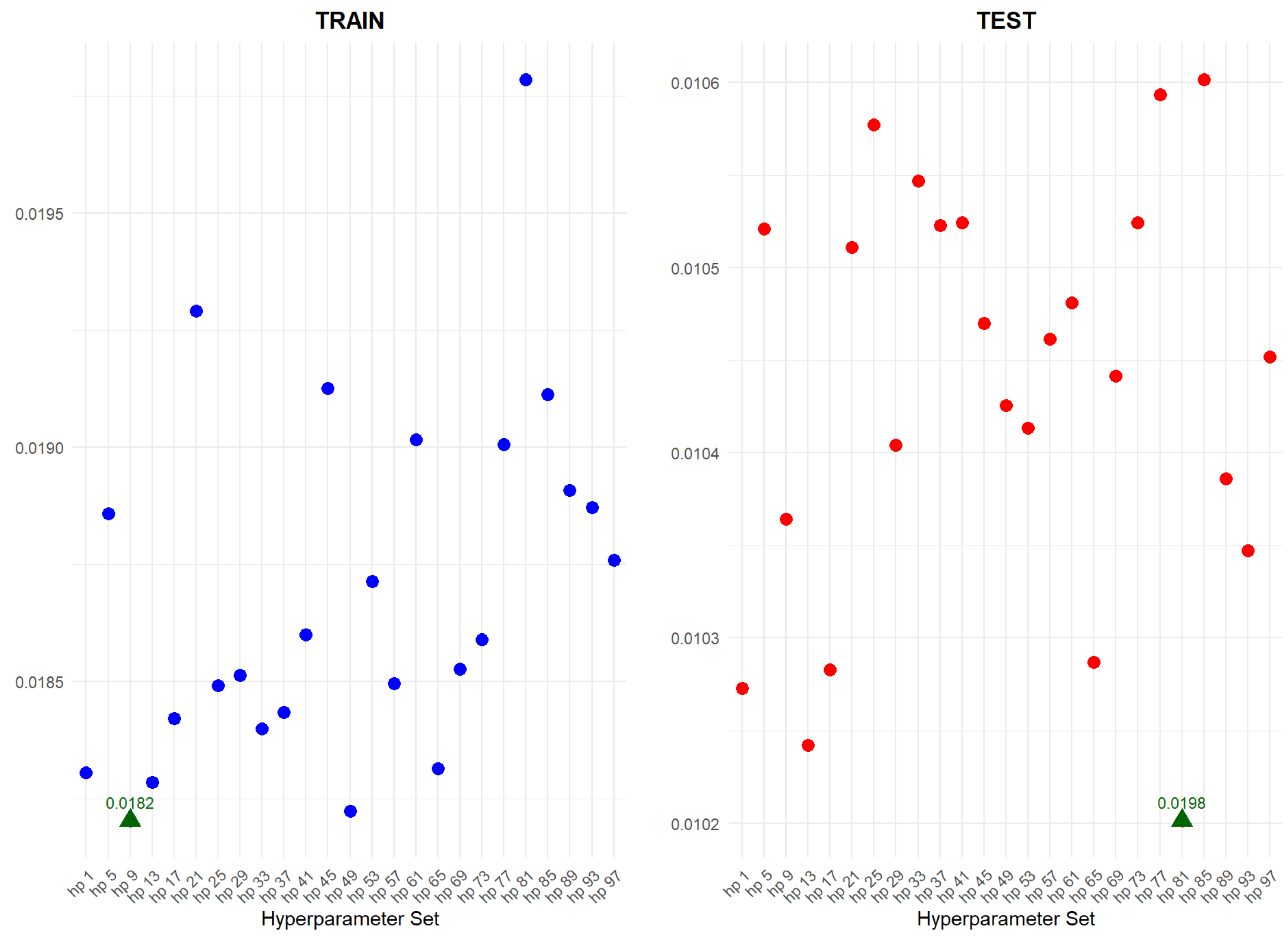
Figure 5.
Efficient Frontier of hyperparameter sets. Model: RF integrated CBD model. Same data set used to in Figure 4.
Figure 5.
Efficient Frontier of hyperparameter sets. Model: RF integrated CBD model. Same data set used to in Figure 4.
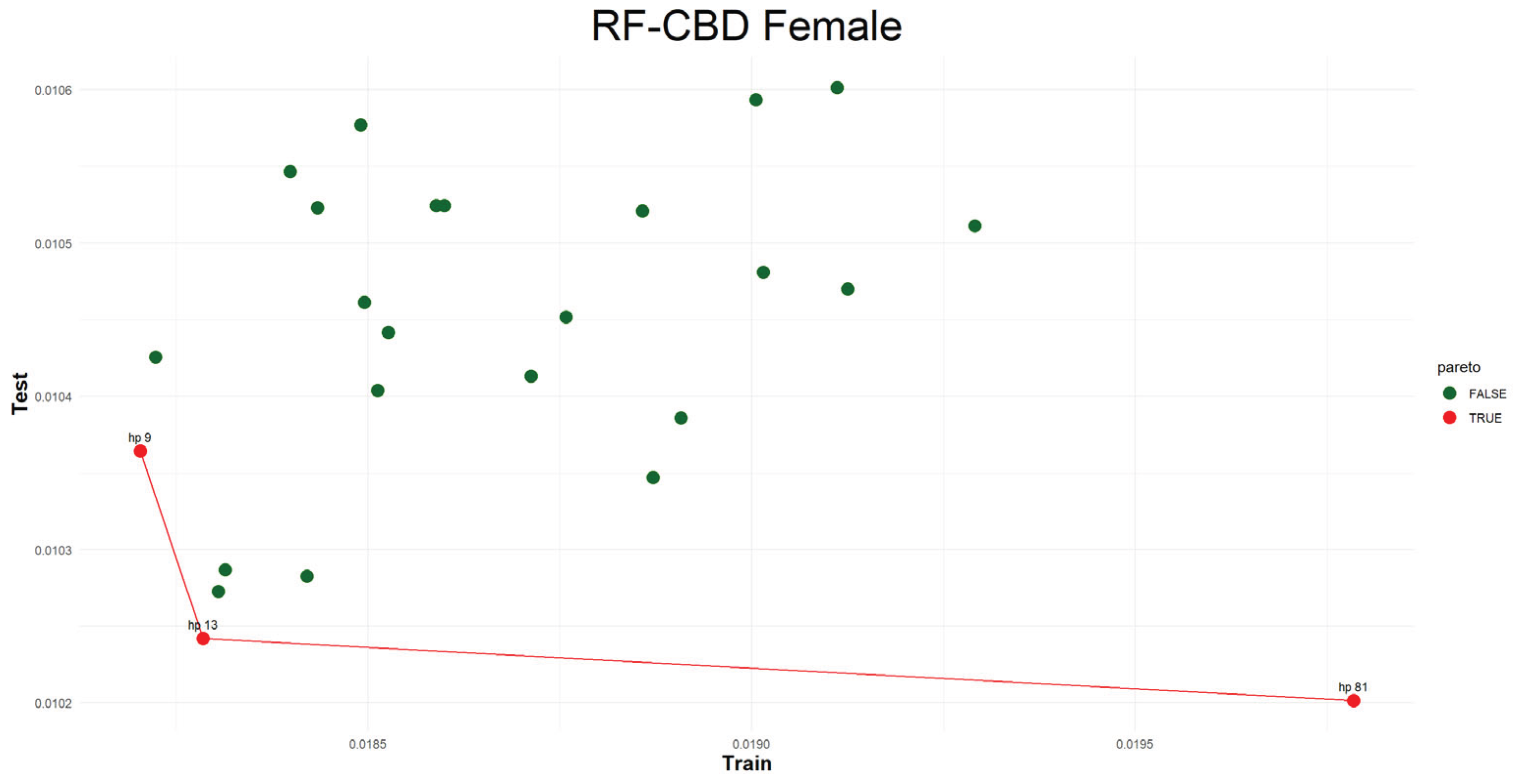
Table 1.
Structure of the stochastic mortality models.
| Mortality Model | Short Definition | Structure |
|---|---|---|
| Lee-Carter (LC) | Static age function, an age-period term, no cohort effect. | |
| Renshaw-Haberman (RH) | Generalizes LC by adding cohort effect. | |
| Age-Period-Cohort (APC) | Basic form of age-period-cohort models. | |
| Cairns-Blake-Dowd (CBD) | Two age-period terms, no static age function, no cohort effect. | |
| M7 | CBD with quadratic age effect and a cohort effect. | |
| Plat | Hybrid version of LC and CBD. |
where, |
Table 2.
Minimum RMSE value of the testing period with corresponding1 RMSE of the training period and minimum RMSE value of the training period*.
Table 2.
Minimum RMSE value of the testing period with corresponding1 RMSE of the training period and minimum RMSE value of the training period*.
| Pure | DT | RF | GB | XGB | ||||||||||
|---|---|---|---|---|---|---|---|---|---|---|---|---|---|---|
| Min Test | Min Train | Min Test | Train | Min Train |
Min Test | Train | Min Train |
Min Test | Train | Min Train |
Min Test | Train | Min Train |
|
| LC | 0.8084 | 2.1349 | 0.7615 | 1.9795 | 1.2229 | 0.7635 | 1.1311 | 0.8207 | 0.7668 | 1.9176 | 1.8477 | 0.7547 | 1.6795 | 1.3928 |
| CBD | 1.0778 | 2.6752 | 0.9048 | 1.9989 | 1.4155 | 1.0201 | 1.9784 | 1.8203 | 0.9776 | 2.0735 | 1.8669 | 1.0075 | 1.7899 | 1.4575 |
| APC | 1.7488 | 2.4273 | 1.3095 | 2.0338 | 2.0338 | 1.0152 | 1.1911 | 0.8452 | 1.0411 | 1.8730 | 1.8061 | 0.9701 | 1.3537 | 1.3537 |
| RH | 1.0053 | 1.9992 | 1.0001 | 1.4051 | 1.4051 | 0.8101 | 1.2610 | 0.8504 | 0.9330 | 1.8479 | 1.7672 | 0.7681 | 1.8907 | 1.3177 |
| M7 | 2.7858 | 1.9877 | 2.4128 | 1.9242 | 1.9198 | 2.4457 | 1.2030 | 0.8489 | 2.3781 | 1.7950 | 1.7824 | 1.9853 | 1.8368 | 1.2736 |
| Plat | 2.1286 | 2.0379 | 1.8430 | 1.9432 | 1.9277 | 1.9029 | 1.2281 | 0.8454 | 1.8686 | 1.7536 | 1.7536 | 1.5092 | 1.9064 | 1.2454 |
*: Results are multiplied with 102 to make them fit the table. 1Train results show the value of the hyperparameter set used over the training period which finds the minimum RMSE over the test period.
Disclaimer/Publisher’s Note: The statements, opinions and data contained in all publications are solely those of the individual author(s) and contributor(s) and not of MDPI and/or the editor(s). MDPI and/or the editor(s) disclaim responsibility for any injury to people or property resulting from any ideas, methods, instructions or products referred to in the content. |
© 2025 by the authors. Licensee MDPI, Basel, Switzerland. This article is an open access article distributed under the terms and conditions of the Creative Commons Attribution (CC BY) license (http://creativecommons.org/licenses/by/4.0/).
Copyright: This open access article is published under a Creative Commons CC BY 4.0 license, which permit the free download, distribution, and reuse, provided that the author and preprint are cited in any reuse.


