Submitted:
25 August 2025
Posted:
27 August 2025
You are already at the latest version
Abstract
This paper will consider the behavior of the velocity obtained from the static spherically symmetric metric resulting from the square lagrangian of f(R) gravity. Metric is given by E. Pachlaner and R. Sexl in their paper [1]. Also It will be shown the expressions for radial and total velocity of cosmos in one and two space dimensions and to discuss their behavior. The metric obtained from the lagrangian which is different from Einstein’s by the square term of the Ricci scalar. The exact equations of fields are too complicated to be solved, it solved in weak field approximation.
Keywords:
relativity and gravitational theory
; equations of motion
; exact solutions
; approximation procedures
; weak fields
1. Introduction
1.1. Equation of Field
In this work has been considered velocity of cosmos in one and two space dimensions and try to find the behavior of radial and total velocity of cosmos. Action integral which proposed by E. Pachlaner and R. Sexl in their paper [1] is:
where k is Einstein gravitation constant. a is constant of dimension of length and R is Ricci scalar. is action integral of matter fields. They calculated the field equations from the variation metric elements in the action integral and solve them for a point mass at rest at the origin. They used the weak field approximation to solve problem and get following equation [1]:
They used centrally symmetric field and introducing polar coordinates to get next equation [1]:
After they had solved equations, they got two solutions [1]: first for
and second for
where is Schwarzschild radius, G is gravitational constant, c is light of velocity and M is mass of center of gravitation and is indefinite constant. For solar system, Schwarzschild radius is 2.95 km and it is much less than distance between Sun and Earth. Because the solution is indefinite and strongly oscillating for , they decided to continue with first solution where .
1.2. Metric
After they had solved equations of field, they got for the line element next static spherically symmetric metric [1]:
where A, B and C are functions of radius r.Metric elements of metric tensor are given [1]:
where are
and
The metric presents a spherically symmetric spacetime in general relativity.
Cristoffel symbols are given by next expression:
where are
Also the following notations are used , , and
The general form of geodesic equations without external field is given by next expression [2]:
Geodesic equations are differential equations for the four space-time components: , where p is affine parameter describing the trajectory. The geodesic equations represent freely moving bodies in spacetime. The equations of field can be derived from the geodesic equation, which is a second-order differential equation. Geodesic equations present the trajectories of bodies moving under the influence of gravity. The form of the geodesic equations will depend on the coordinate system and the metric coefficients , , and . The line element describes a curved spacetime. In general relativity, the motion of objects is generated by the curvature of spacetime which is determined by gravity.
1.3. Gravitation Potential and Fifth Force
In the weak field limit, gravitational potential may be written [2,3]:
where A is 00 component of metric tensor.
In this case gravitation potential has next shape :
and it is a similar with the potential of fifth force [5]. The fifth force was used by Ephraim Fischbach to explain experimental deviations in the theory of gravity. Some scientists consider the fifth force to be a type of fundamental interaction such as the four interactions in nature: gravitational, electromagnetic,strong nuclear, and weak nuclear forces.
The fifth force should explain astronomical observations that predict corrections to the theory of gravity.
The term fifth force was mentioned in a 1986 paper byEphraim Fischbach and coauthors. The paper discussed the results obtained in Eotvos (Eötvös) experiment of Lorand Eotvos (Loránd Eötvös) at the beginning of the 20th century and they presented that we need to modify the gravity inverse square law [6,7].
Fuji considered in his 1971 paper the modification of the gravitational force and proposed that the distance dependence of the force could be corrected by introducing a term similar to the Yukawa potential [8,9].
The magnitude of the strength of the interaction in above equation is given by parameter 1/3 [7].
In the paper of Fischbach presented that the the strength of the interaction is around 1/100 of gravity and the range of the interaction is a few hundred meters [10].
Discreapance between models of general relativity and quantum field theory and between the cosmological constant problem and hierarchy problem led to the introduction of a fifth force [7].
2. Geodesic Equation and Velocity of Cosmos
2.1. Cristoffel Symbols
Cristoffel symbols different from zero for static spherically symmetric metric proposed by E. Pachlaner and R. Sexl are [4]:
2.2. Geodesic Equations in Four Dimensions
2.3. Geodesic Equation in Two Dimensions and Velocity of Cosmos
In one space dimension, geodesic equations are given by following relations.
First equation is:
First equation becomes:
Second equation is:
Second equation becomes:
Velocity in one space dimension is: .
2.4. Geodesic Equation in Three Dimensions and Velocity of Cosmos
In two space dimensions, geodesic equations are:
First and third equation become:
Substitution first and third equations in second equation following expression will be obtained:
where are
Equation becomes:
where are
Substitute first and second derivates in equation we get:
Solving above equation we get:
Substitute functions and , the following expression is obtained for radial velocity
Radial velocity is ,
Transverse velocity: .
3. Results and Discussion
3.1. Radial Velocity in Two Dimensions
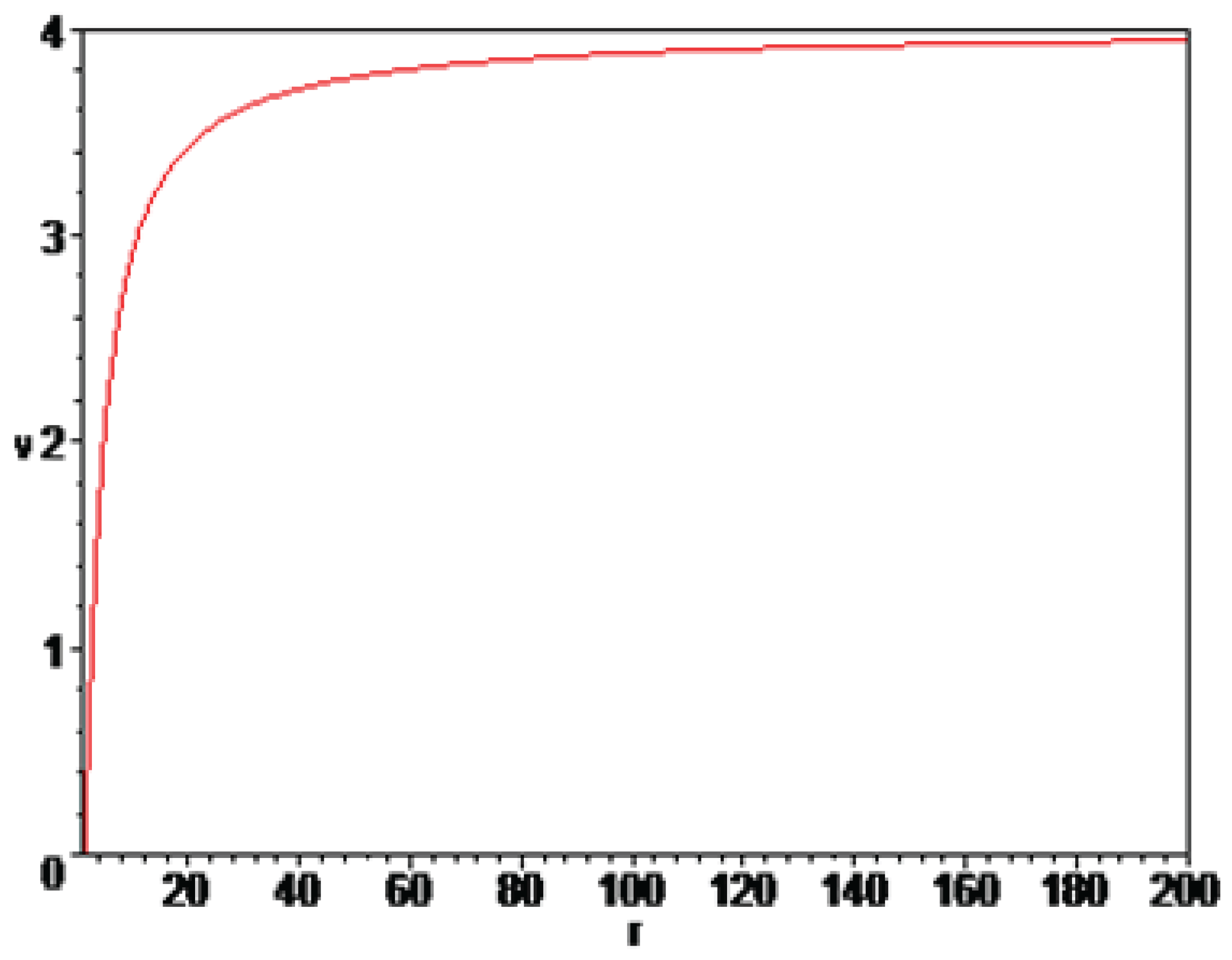
Radial velocity in two dimensions (one space dimension and one time dimension) E. Pachlaner and R. Sexl metric are given by following equation:
On the next two pictures Figure 1 and Figure 2 are shown velocity in two dimensions for different value of parameter K. The first picture are very similar to Newton’s behavior of the galaxy rotation speed curves and the second image is very similar to the behavior of rotational speed curves as proposed by Vera Cooper Rubin. Gravitational law of Newton gives that the stars near galactic center rotate faster than the stars futher from the galactic center as shown on the Figure 1. Meanwhile the observations of galaxy rotation curves predict that the stars in outer shells of galaxies have got constant orbital speed as on Figure 2. The difference between Newton prediction and observations can be explaned by the existence of dark matter and dark energy. Besides dark matter and dark energy there are many theories which proposed to change Newton law of gravitation to explain rotation curves. One of this theories is the introduction of fifth force as mentioned in first section of this paper. It should be mentioned that the velocity results in all four images are normalized to the speed of light.
3.2. Radial and Transverse Velocity in Three Dimensions
Radial velocity in three dimensions (two space dimensions and one time dimension) E. Pachlaner and R. Sexl metric are given by following equation:
where are:
The transverse velocity in three dimensions E. Pachlaner and R. Sexl metric are given by following equation:
As can be seen in Figure 3, the transverse velocity decreases sharply with distance accoording to a hyperbolic law. It can be concluded that transverse velocity does not significantly affect on the total velocity of spread cosmos. As we can see in Figure 4, the radial velocity has a significant value at large distances which is approaching some saturation velocity. It can also conclude that the radial velocity curve has a similar shape as in Figure 2, for the model of one space dimension. The expression for radial velocity in one space dimension is different from the expression in two space dimensions by the term containing and that term is much smaller than others terms. So we can conlude that the correction in the expression for velocity in three dimensions is quite small, and the radial velocity curves are similar in two and three dimensions.
The Figure 5 shows the square value of radial velocity and the Figure 6 shows the sum of square value of the radial velocity and the square value of the of transverse velocity. As can be seen Figure 5 and Figure 6 are similar, that is, the transverse velocity is very small compared to the radial velocity. So we can conclude that the total velocity is equal to the radial velocity in two dimensions of space.
Author Contributions
The paper has one author. In the first section the historical development of the topic is presented. Also it is used AI Assistant for some historical facts as fifth force. The program Maple V Release 5 (from 1996 year) or Maple 2018 used to check expressions for Christopher symbols and geodesic equations in four dimensions and draw images. The section two and section Results and Discussion are the independent work of author.
Funding
This research received no external funding.
Acknowledgments
This work is supported by Ministry of Science, Technological Development and Inovations of the Republic of Serbia Nr. 451-03-136/2025-03/200017
Conflicts of Interest
The author declare no conflict of interest.
Abbreviations
The following abbreviations are used in this manuscript:
| A | A(r) |
| B | B(r) |
| C | C(r) |
Appendix A. Solving the Second Geodesic Equation in Two Space Dimensions
Our goal is to solve next differential equation:
to get expression for velocity in two space dimension cosmos. We need make inverse differential equation to use next substitutions:
and we get next equation:
To solve above equation we will use following calculation steps.
First the equation will be multiple by factor and we get:
i.e.
Then we use substitution , and we get
Then we make new substitution , also
Our equation becomes:
Then we finally get the next expression:
References
- Pechlaner, E..; Sexl, R..; On Quadratic Lagrangians in General Relativity., Commun. math. Phys., 1966, 2, 165–175. 10.1007/BF01773351.
- Lazarov, N. Dj.; Borka Jovanovica, V.; Borka, D.; Jovanovic, P.; Geodesic equations in the weak field limit of general f (R) gravity theory., Filomat, 2023, 37-25, 8575–8581. [CrossRef]
- Lazarov, N. Dj.; Forgiarini, I.; Geodesic equations of Weyl conformal gravity theory in CSS metric., Filomat, 2024, 38-4, 1451–1464. [CrossRef]
- Weinberg, S.; Gravitation and Cosmology; ISBN 0-471-92567-5.; John Wiley and Sons: New York, USA, 1972; pp. 32–58.
- Borka, D.; Borka Jovanovica, V.; Nikolic, V.N.; Lazarov, N. Ð.; Jovanovic, P.; Estimating the Parameters of the Hybrid Palatini Gravity Model th the Schwarzschild Precession of S2, S38 and S55 Stars: Case of Bulk Mass Distribution Universe, 2022, 8, 70. [CrossRef]
- Fischbach, E.; Sudarsky, D.; Szafer, A.; Talmadge, C.; Aronson, S.H.; Reanalysis of the Eötvös experiment., Physical Review Letters, 1986, 56 (1), 3–6. [CrossRef]
- Safronova, M. S.; Budker, D.; DeMille, D.; Kimball, D. F. J.; Derevianko, A.; Clark, C. W.; Search for new physics with atoms and molecules., Reviews of Modern Physics., 2018, 90 (2), 025008. [CrossRef]
- Fujii, Y; Dilaton and Possible Non- Newtonian Gravity., Nature Physical Science., 1971, 234 (44) 5–7. [CrossRef]
- Fischbach, E.; Talmadge, C. L.; Search for Non-Newtonian Gravity; Springer New York: New York, USA, 1999.
- Will, C. M. ; The Confrontation between General Relativity and Experiment;Living Reviews in Relativity., 2014, 17, 4. [CrossRef]
- Cicoli, M.; Pedro, F. G.; Tasinato, G.; Natural quintessence in string theory;Journal of Cosmology and Astroparticle Physics., 2012, 7 44. [CrossRef]
- Dvali, G.; Zaldarriaga, M.; Changing α with time: Implications for Fifth-Force-Type Experiments and Quintessence.Physical Review of Letters., 2002, 88 (9) 091303. [CrossRef]
Figure 1.
Radial velocity as a function of radius in Astronomical Units in two dimensions for , , .
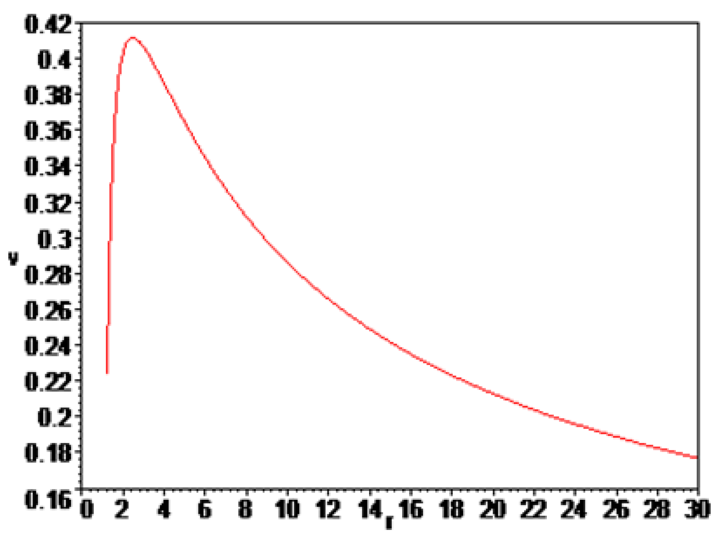
Figure 2.
Radial velocity as a function of radius in Astronomical Units in two dimensions for , , .
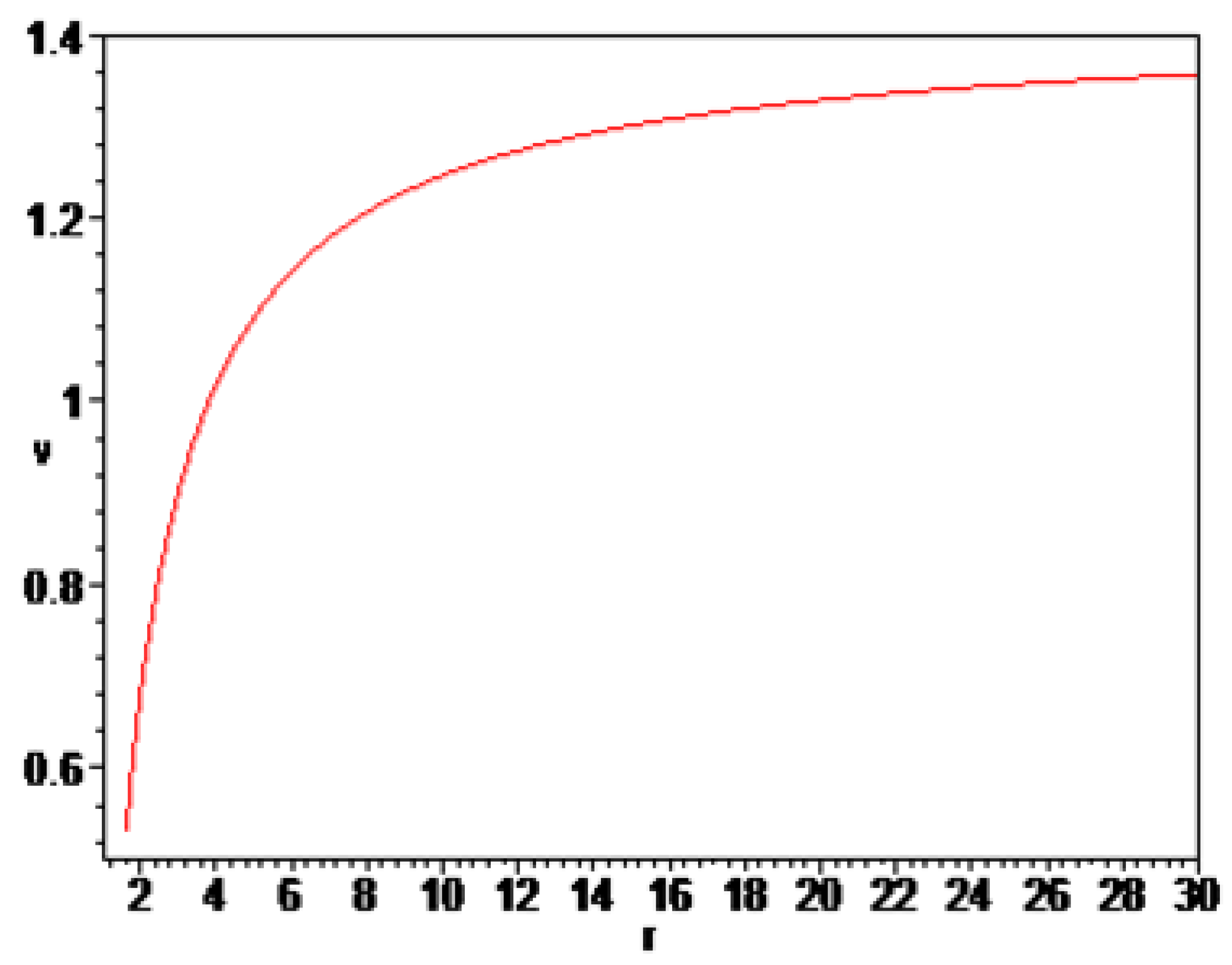
Figure 3.
Transverse velocity as a function of radius in Astronomical Units in three dimensions for , , , .
Figure 3.
Transverse velocity as a function of radius in Astronomical Units in three dimensions for , , , .
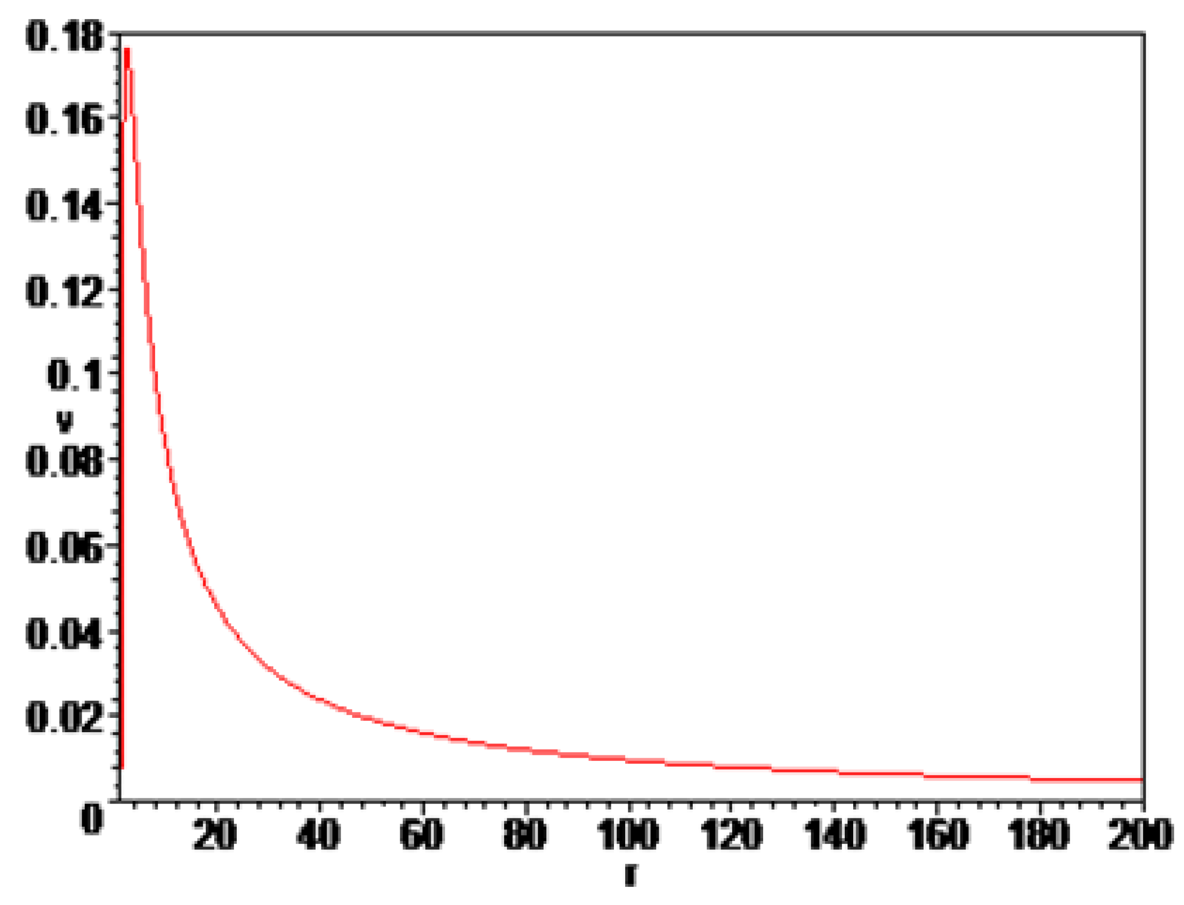
Figure 4.
Radial velocity as a function of radius in Astronomical Units in three dimensions for , , , .
Figure 4.
Radial velocity as a function of radius in Astronomical Units in three dimensions for , , , .
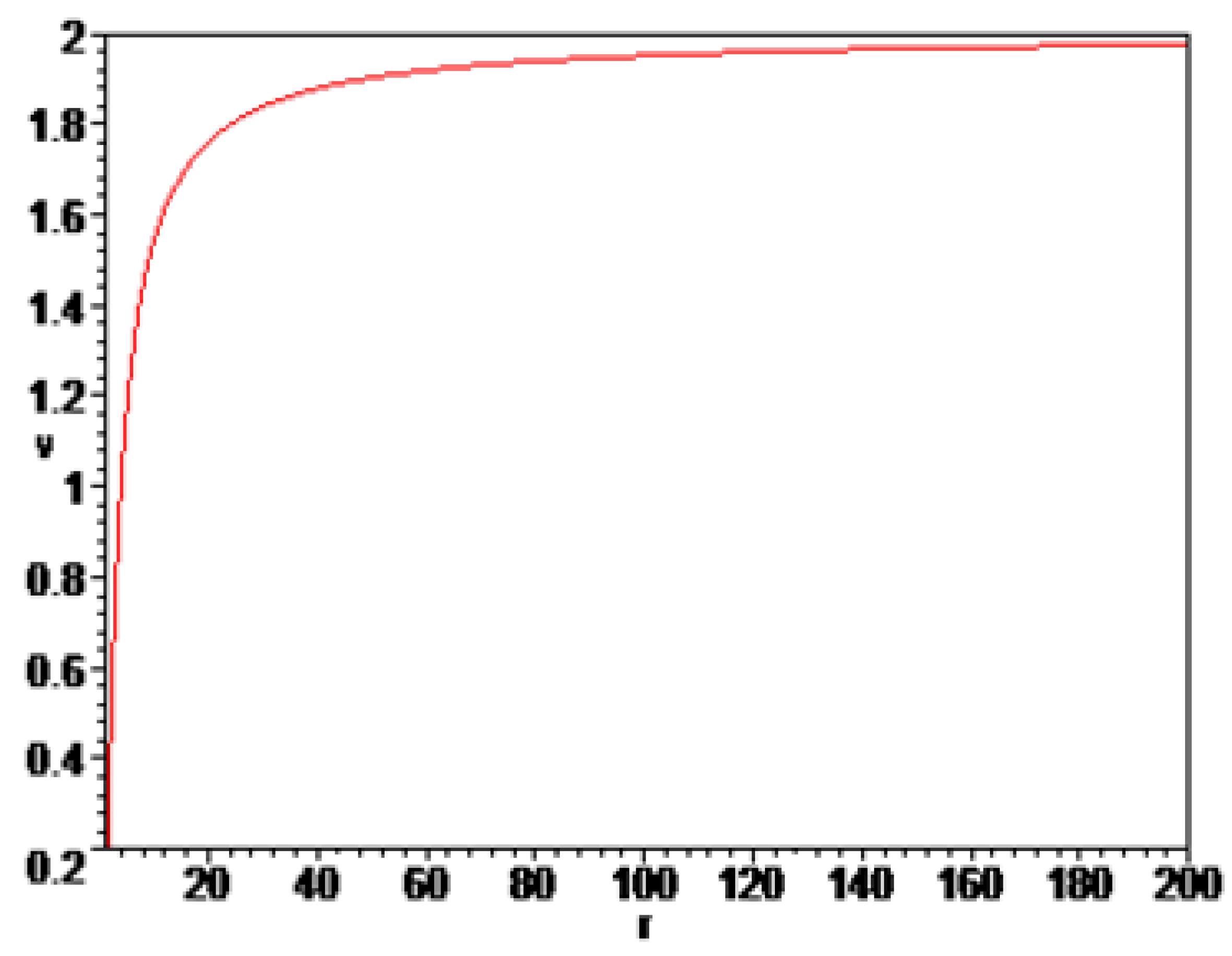
Figure 5.
velocity as a function of radius in Astronomical Units in three dimensions for , , , .
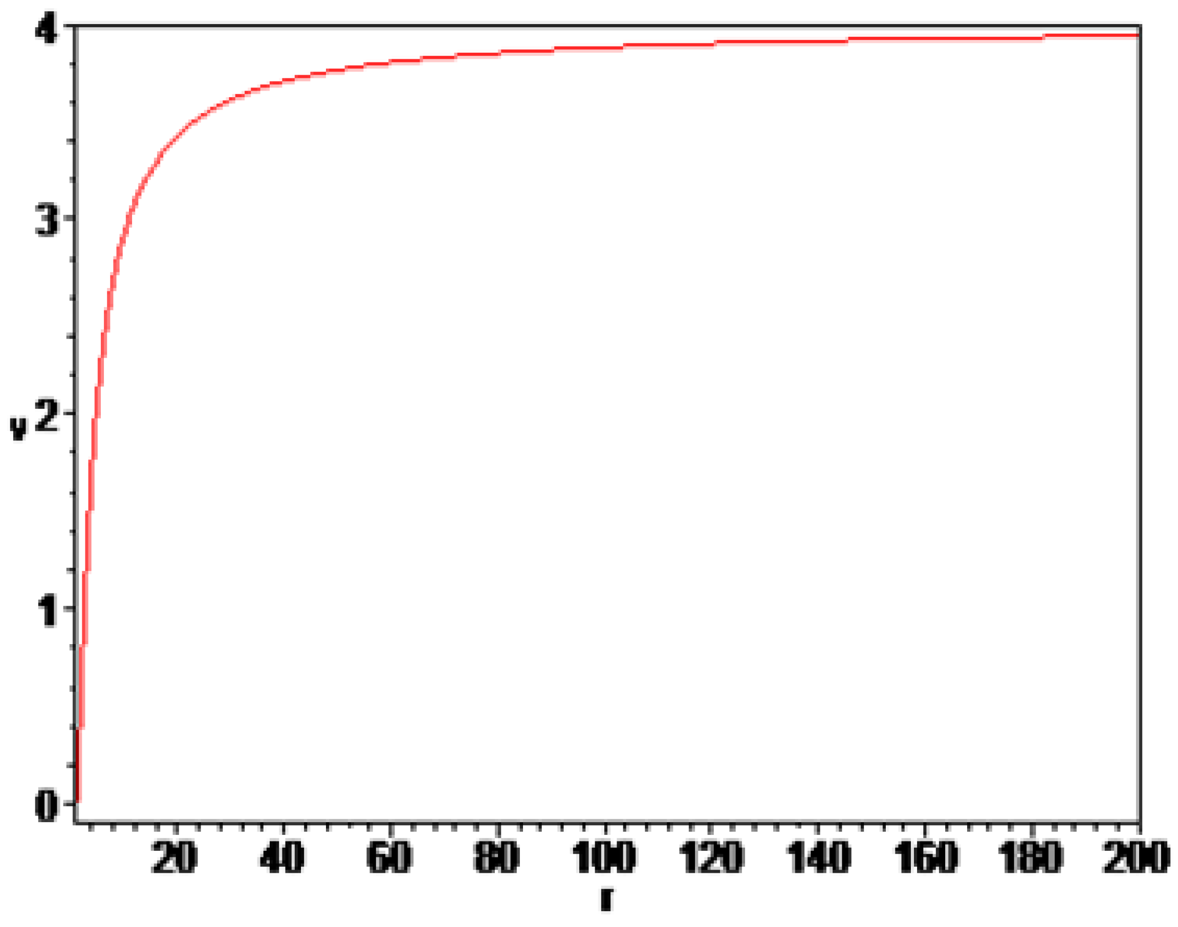
Figure 6.
velocity as a function of radius in Astronomical Units in three dimensions for , , , .
Disclaimer/Publisher’s Note: The statements, opinions and data contained in all publications are solely those of the individual author(s) and contributor(s) and not of MDPI and/or the editor(s). MDPI and/or the editor(s) disclaim responsibility for any injury to people or property resulting from any ideas, methods, instructions or products referred to in the content. |
© 2025 by the authors. Licensee MDPI, Basel, Switzerland. This article is an open access article distributed under the terms and conditions of the Creative Commons Attribution (CC BY) license (http://creativecommons.org/licenses/by/4.0/).
Copyright: This open access article is published under a Creative Commons CC BY 4.0 license, which permit the free download, distribution, and reuse, provided that the author and preprint are cited in any reuse.


