Off-Diagonal Decoupling and Integrability of (Non) Metric Geometric Flow and Finsler-Lagrange-Hamilton Modified Einstein Equations

1. Introduction: Metric and Nonmetric Finsler-Lagrange-Hamilton Geometric Flows, GR and MGTs

The general relativity (GR) theory, i.e. Einstein’s gravity, is considered by the bulk of researchers as the almost standard theory of gravity beginning the end of 1915, when A. Einstein and D. Hilbert completed the formulation of gravitational field equations in certain heuristic and, respectively, variational forms. The monographs [1,2,3,4] contain summaries of results and methods, and the most important cosmological and astrophysical applications of GR before the "accelerating cosmology era". The Einstein gravity theory was formulated axiomatically on Lorentz manifolds defined as relativistic versions of the (pseudo) Riemannian spaces, when various types of metric, tetradic (vierbeind) and spinor variables and 3+1 or 2+2 nonholonomic decompositions were used. The discovery of late-time cosmic acceleration [5,6] resulted in extensive research on modified gravity theories (MGTs) [7,8,9,10,11] and dark energy (DE) and dark matter (DM) physics [12]; and on geometric and quantum information flows [13], see references therein. In this work, we do not cite many works on non-Riemannian geometries and related MGTs and do not discuss certain models if they do not consider nonholonomic or Finsler geometry methods in explicit forms. For reviews of results and geometric methods, readers are recommended to study [14,15,16] and references therein.

Finsler-like generalizations of the Einstein gravity form a special class of MGTs when the geometric and physical objects depend not only on some base manifold coordinates but also on so-called velocity/momenta type coordinates (for different types of models with local anisotropies). We studied such relativistic Finsler-Lagrange-Hamilton (FLH) geometries and MGTs modelled on (co) tangent Lorentz bundles. We also elaborated on higher order tangent bundle, supersymmetric, nonassociative and noncommutative and other type extensions as we reviewed in chronological form in [13,17,18]. Here, we provide and review an extended list of our contributions to both metric-compatible and noncompatible FLH theories and elaborate on new methods of constructing exact solutions for nonmetric MGTs. Many such works were published during 1988-2008 in Eastern Europe [19], being less known and not correspondingly cited in Western countries.

This paper can be considered as a status report and a transfer of knowledge on geometric methods for constructing exact and parametric solutions in FLH theories. It also consists a review and a pedagogical introduction into the anholonomic frame and connection deformation method, AFCDM, formulated for constructing off-diagonal solutions in relativistic Finsler geometric flow and gravity models. This work is different from the nonassociative and noncommutative FLH theories (on eight dimensions, 8-d, tangent and cotangent Lorentz bundles) studied in Part II of [18]. Here we consider real associative and commutative and nonmetric theories on nonholonomic phase spaces involving conventional velocity or momentum like coordinates. It redefines for Finsler theories the 4-d constructions from Part I (and respective Tables) of that review article and of recent published papers on off-diagonal solutions and G. Perelman’s thermodynamics [20,21]. Here we note that a series of early results and geometric methods on constructing off-diagonal solutions in GR and Finsler and non-Finsler MGTs were reviewed in [22,23,24,25,26].

1.1. Historical Remarks on Finsler-like Relativistic Geometric Flow and Gravity Theories

We list and discuss seven most important steps to formulating and further developments of respective directions in FLH geometry and physics, which are important for the objectives of this work:

[1] 

Prehistory and beginning of History (1854-1934): B. Riemann considered in his famous habilitation thesis ([27], 1854) the first example of nonlinear quadratic element $d{s}^2=F^2(x,y),$ where $x=\left\{x^i\right\}$ are coordinated on a base manifold V and $y=\left\{y^a\right\}$ are certain fibler/velocity like coordinates. Such an $F(x,y)$ involving homogeneity conditions on y (when $F(x,\lambda y)=\lambda F(x,y),$ for $\lambda >0$), was later called a Finsler metric, or (equivalently) a Finsler generating function. The Riemannian geometry was formulated and studied by using quadratic elements, $d{s}^2\simeq g_{ij}\left(x\right)y^i{y}^j,$ for $y^a\simeq d{x}^a,$ and a symmetric metric tensor $g_{ij}\left(x\right).$ That was the "prehistory" of Finsler geometry.

− The "Finsler history" began in 1918 due to P. Finsler’s thesis [28], when the term "Finsler geometry" was introduced in E. Cartan’s first monograph on Finsler geometry from 1935 [29]. In that monograph (in coordinate form), the first examples of Finsler nonlinear, $\tilde{\mathbf{N}}=\left\{{\tilde{N}}_i^a(x,y)\right\},$ connection (N-connection) and linear distinguished connection (d-connection) $\tilde{\mathbf{D}}=\left\{{\tilde{\mathbf{D}}}_{\alpha }(x,y)\right\}$ were considered. Such values consist of two other cornerstone geometric objects (the first one is $F(x,y)$). Mathematical details on so-called Riemann-Finsler geometry can be found in monographs [30,31,32]. We consider that E. Cartan’s contributions are also fundamental because without his first use of N- and d-connections and the concept of bundle space, Finsler geometric and physical models are incomplete for elaborating applications in physics. For our purposes to formulate and study relativistic Finsler generalizations of the Einstein gravity theory and to construct exact and parametric solutions in such theories, we follow the system of notations and conventions stated in [13,17,19].1

[2] 

Classical Geometric Ages (1935 - 1955): A series of fundamental geometric papers were published on so-called metric noncompatible Finsler geometry theories due to L. Berwald [33,34] and S. -S. Chern [35] and others. Such Finsler geometric models are different from the Finsler-Cartan theories and involve many conceptual and technical difficulties in elaborating Finsler modifications of GR and standard particle physics because of nontrivial nonmetricity fields, as we criticised in [17,19,36]. For instance, it is a problem how to define Finsler-spinors and Finsler-Dirac equations, conservation laws, and finding exact and parametric solutions of respective locally anisotropic modifications of the Einstein equations. In principle, a cure exists as in the case of metric-affine gravity theories formulated on (co) tangent Lorentz bundles following advanced geometric methods for constructing generic off-diagonal solutions as in [37]. For FLH MGTs, this is a task for a series of future works.

− We also mention certain important works on the geometry of nonholonomic manifolds due to G. Vrǎnceanu and Z. Horak (1926-1955) [38,39,43]; and on the global theory of N-connections and Finsler geometry due to A. Kawaguchi (1937-1952) [40,41] and C. Ehresmann (1955) [42]. Summaries of results and detailed bibliography on the classical period of Finsler geometry and first applications can be found in [17,19,30,31,32].2 We can consider that all FLH models consist of particular examples of nonholonomic manifolds or (co) tangent bundle geometries defined by respective N-connection structures.

[3] 

Early Middle Ages (1950 - 1974): That was the beginning of research on applications of Finsler geometry methods in MGTs and geometric mechanics. For our purposes, we mention the first Finsler modification of the Einstein equations, when instead of the Levi-Civita (LC) connection ∇ the Cartan distinguished (d) connection $\tilde{\mathbf{D}}$ was used (J. I. Horvath, 1950) [44]. We also cite the monograph [45], which contains a rigorous formulation of Finsler geometry as an example of (co) tangent bundle geometry. It is defined by Sasaki lifts of Hessians (vertical quadratic forms $\sim {\partial }^2{F}^2/\partial y^a\partial y^b$), using N-connections, to total metrics $g_{\alpha \beta }$ on $TV.$ In our opinion, such constructions are very important because they result in well-defined geometrically complete d-metrics on (co) tangent Lorentz bundles and allow self-consistent extensions of metrics in GR.

[-$3.1$] Relativistic Lagrange mechanics as a generalized Finsler geometry without homogeneity conditions, on tangent Lorentz bundle. Another very important work was that due to J. Kern (1974) [46] who introduced the concept of Lagrange geometry with nonlinear quadratic element $d{s}^2=L(x,v)$ on a tangent bundle $TM.$ This provides an alternative geometrization of classical mechanics which is different from the standard approach to geometric mechanics (see, for instance, [47]). Finsler geometry is a particular example of homogeneous mechanics, when $L=F^2.$ Such generalizations are very important because Finsler metrics with homogeneity conditions consists of a very special case, which is not motivated for general nonlinear interactions and MDRs in MGTs or GR.

-$[3.2]$ Relativistic Hamilton mechanics as a cotangent Lorentz bundle model of generalized Finsler geometry and equivalent almost (symplectic) Kähler-Lagrange/ Hamilton.Using Legendre transforms, $L(x,v)\to H(x,p),$ the concept of Hamilton geometry, with nonlinear quadratic elements $d{⁤}^{|}{s}^2=H(x,p)$, on cotangent bundle $T^{*}M,$ can be introduced. Such geometries can be constructed on Lorentz manifolds with nontrivial N-connection structures and described equivalently as almost (symplectic) Kähler-Lagrange/ Finsler (or Kähler-Hamilton/geometries, see [31,48,49,50]). Respectively, classical and quantum geometric techniques are important for the deformation quantization for such theories [17,51,52,53,54] (in chronological form, such developments are relevant to the research described for directions 6-7], see below).

[4] 

Middle Ages (1959 - 1995): The period is characterized by many works on Finsler and other types of locally anisotropic field theories and gravity. It begins with the publication of the monograph [30] (H. Rund, 1959). It was translated into Russian by G. Asanov, who developed (together with his postgraduate students, during 1980-1990) in the former USSR some new directions with applications in physics of Finsler geometry [55,56,57]. M. Masumoto’s monograph [31] (1986) played a very important role in the elaboration of various variants of Finsler gravity theories and postulating certain versions of Finsler gravitational field equations [58,59,60,61,62,63,64,65]. At that time, certain methods of constructing solutions of locally anisotropic gravitational field equations were not formulated, but only certain post-Newtonian computations of possible Finsler anisotropy effects.

[5] 

Dark non-standard Ages (1975 - 2011): It was an "Orthodox" period of GR and standard particle physics, when influential authors in gravity and QFT [66,67] concluded that Finsler theories with generic anisotropies had substantial restrictions by experimental and observational data. Their theoretical analysis had not involved nontrivial N-connection structures, which made those conclusions quite uncertain and ambiguous. Unfortunately, because of the mentioned works, tents of Finsler papers (including manuscripts by this author) were rejected from Phys. Rev. Lett. and Phys. Rev. D as "as unphysical". That situation was described in Appendix B of the preprint variant of [17], see also references therein. Nevertheless, many authors in the USA, Japan, Germany, UK, Canada, Greece, Russia, Poland, Romania, R. Moldova, etc., published in other mathematical and theoretical physics journals of number of papers on generalized Finsler gravity theories [17,68,69,70]. Here we note that important works (using the FLH geometric methods) were performed using nonholonomic fibered structures on Lorentz manifolds, in extra-dimension gravity, string theory, noncommutative Finsler gravity, etc. [71,72,73,74,75]. A series of important monographs on nonholonomic manifolds and generalized Finsler gravity and applications were published [19,50,62,64,76,77].

[6] 

Renaissance (1996 - 2011): The period is characterized by a new series of works on modified dispersion relations (MDRs) and local Lorentz invariance violations (LIVs) as attempts to solve certain important problems in QG, string theory and other MGTs [78,79,80]. For additional assumptions on nonholonomic geometric structures, various classes of such theories can be formulated as (generalized) Finsler geometries. This induced in the literature a non-correct opinion that Finsler gravity models are theories with local anisotropies determined by MDRs and LIVs [81,82,83,84].

-$[6.1]$ Elaborating general methods for constructing exact and parametric solutions in FLH MGTs. As we mentioned above, FLH geometric and physical models can be formulated in general self-consistent forms on (co) tangent Lorentz bundles when the postulates of GR theory can be extended from similar ones with Lorentz manifolds [17,19,85]. Using nonholonomic methods as in Finsler geometry, redefined in canonical 2+2 variables on Lorentz spacetimes, we can construct new classes of off-diagonal exact and parametric solutions in GR and MGTs. Extending the constructions to higher dimensions involving nonholonomic dyadic decompositions and distortions of affine (linear) connections, the anholonomic frame and connection deformation method (AFCDM) was formulated [23,24,25,86,87,88]. Perhaps, this is the most general geometric and analytic method which allows us to decouple and integrate in certain general forms the gravitational and matter field equations in FLH and other types of MGTs, and GR, see recent reviews and results [13,17,26]. The ansatz for constructing such solutions is chosen as some generic off-diagonal metrics that depend on the type of distorting relations for connections, and on prescribed generating sources.

-$[6.2]$Problems with the definition of Finsler-spinors and Finsler-Dirac equations. Another fundamental problem for elaborating physically viable FLH is that of formulating Finsler generalizations of the concept of Clifford structures/ spinors adapted to N-connection structures. A related issue is that on how to formulate self-consistent variants of Finsler-Dirac equations, and (in general) to construct FLH modifications of the Einstein-Yang-Mills-Higgs-Dirac (EYMHD) equations. Such research programs were performed for metric compatible Finsler connections (during 1996 - 2012) in our works [19,62,64,89,90,91,92,93,94,95,96,97]. We criticized [17,19,36] the approaches for elaborating nonmetric Finsler gravity theories (involving Chern, Berwald and other type metric noncompatible Finsler connections). That was because of ambiguities with the definition of nonmetric versions of the Finsler-Dirac equations and with the formulation of conservation laws for nonmetric FLH deformed EYMHD systems. Such difficulties do not exist for the case of Finsler-Cartan geometry, and for FLH generalizations with metric-compatible Finsler connections. Recently, we discussed how to find a cure for nonmetric MGTs using physically important solutions as in [37,98]. One of the main purposes of this work is to show how the AFCDM can be applied both to metric and nonmetric FLHs modified Einstein equations with general generating sources. Proofs of the integrability of nonmetric FLH deformed EYMHD equations will be provided in our future works.

-$[6.3]$ FLH MGTs and string gravity, locally anisotropic gauge gravity, supersymmetric and noncommutative Finsler models. The works [13,26,54,62,71,72,73,74,99,100] contain a series of original results on Finsler like (super) string and supergravity theories formulated for extra dimension coordinates being of velocity/ momentum type. The approach was developed for noncommutative Finsler gravity models, Finsler-Hořava-Lifshitz theories, almost Kaehler-Finsler models, deformation and gauge-like quantization of Finsler gauge gravity theories etc. [17,22,101,102,103,104,105]. The AFCDM was correspondingly generalized and applied to constructing physically important solutions in such FLH theories.

-$[6.4]$ Metric and nonmetric nonholonomic and generalized Finsler geometric flows. This direction of our research (see reviews [13,37,106,107]) was inspired by G. Perelman’s preprint [108] on the entropy of Ricci flows and related proof of the Poincaré-Thurston conjecture, see mathematical methods in [109,110,111,112]. Formulatig Finsler generalizations (in a certain unified form of that conjecture) is not possible because of the various types of Finsler geometries. This is different from the case of Riemannian or Kähler geometry. Nevertheless, we can construct abstract geometric and N-adapted variational forms of FLH geometric flow models by using distortions of connections. The most important motivation to formulate such Finsler-like generalizations is that the concepts of G. Perelman W-entropy, and respective statistical and geometric thermodynamic variables, can be computed for any type of FLH geometries and MGTs defined by certain (generalized) Ricci scalar and Ricci tensors. This is enough for analyzing the thermodynamic properties of large classes of exact and parametric solutions in FLH gravity and geometric flow theories. In general, the off-diagonal solutions are not characterized by certain hypersurface, holographic, or duality properties. For such solutions, the Bekenstein-Hawking paradigm [113,114] is not applicable and we have to elaborate on theories of nonholonomic and Finsler geometric flows. Here, we cite our and co-authors’ works beginning 2006, [53,115,116,117,118,119]. Recent results and methods on nonholonomic or nonmetric geometric and quantum information flows and FLH, and other types of MGTs can be found in [13,98,107]. Such works are also related to a series of papers on Finsler-like diffusion, locally anisotropic kinetic processes, locally anisotropic thermodynamics, etc. [17,120,121,122,123,124].

-$[6.5]$ Certain different Renaissance directions were developed by other authors (we reviewed and discussed the most important contributions till 2018 in Appendix B of the preprint variant of [17]). Here we note that those results and methods do not allow for the construction in general forms of certain off-diagonal solutions, depending on the type of Finsler generating functions and prescribed connections. They are different from our approach to FLH and can be incomplete for applying the AFCDM. The fiber (tangent or vector ....) bundle formalism was not applied in elaborating such theories, which put many questions on mathematical rigorous formulation. In many cases, those models and a few found diagonalizable solutions of Finsler-like gravitational equations are with a trivial N-connection structure. Typically, they consist of arbitrary lifts and deformations on y-variables that are not derived as certain exact or parametric solutions involving Sasaki lifts and an axiomatic formulation and self-consistent physical formulation.

[7] 

Nowadays and Future (2012 - ...) After many observational evidences on accelerating cosmology and validating papers of various MGTs and DM and DE physics [5,6,7,8,9,10,11,12], Phys. Rev. D and other influential physical journals began to publish papers on Finsler geometry and applications in modern physics, cosmology and astrophysics [82,125,126,127,128,129,130,131,132,133,134]. New international and multi-disciplinary teams and research groups (originating from Greece, Germany, China, Romania, R. Moldova, Spain, Italy, India, Iran, etc.) have been organized during the last 15 years. We discussed the main developments (till 2018) in Appendix B of the preprint part of [17]. The discovery of late-time cosmic acceleration [5,6] resulted in extensive research on modified gravity theories (MGTs) [7,8,9,10,11] and dark energy (DE) and dark matter (DM) physics [12] Here we analyze in brief some recent results on FLH MGTs and applications, which are relevant to the purposes of this work:

-$[7.1]$ Undetermined concepts of pseudo-Finsler spacetime, causality, and problems with nonmetric Finsler gravitational equations. Such geometric models and possible applications were elaborated in a series of works [125,126,127,133,134,135,136]. This group of authors try to impose a Finsler spacetime standard (publishing in Phys. Rev. D and other influential journals). Former important and more general results and methods (from the periods when Finsler gravity was considered "unphysical") typically are not cited and not discussed, as we described above in 5], and reviewed in [17]). The main idea of the mentioned team of authors was to extend the concept of pseudo-Riemannian geometry in certain causal, with a well-defined theory of observations, and for a concept of pseudo-Finsler spacetime, by postulating a version of locally anisotropic gravitational equations. For instance, such a pseudo-Finsler spacetime can be defined by some data $(V,L=F^2),$ where V is a pseudo-Riemannian manifold and $F(x,v)$ is a Finsler generating function. Additional assumptions are necessary to define certain causality and postulates and to derive in geometric or variational forms some Finsler-like gravitational equations, for instance, of type [125,126], etc. This is not enough for formulating generalizations of Einstein gravity if we do not prescribe some classes of nonlinear and distinguished Finsler d-connections on (co) tangent Lorentz bundles. Well-motivated physical arguments (general theoretic/ phenomenological or observational/experimental one) are necessary for prescribing an F (why it should be homogeneous?) and certain types of N- and d-connections, or to motivate certain very special relativity models. In [127], a procedure on how to make extensions of the Lorentzian spacetime geometry "from Finsler to Cartan can vice versa" is analyzed. Then, in [135], a Birkhoff theorem was proved for Berwald-Finsler spacetimes. Nevertheless, Berwald, Chern or other type of nonmetric d-connections (reviewed in [136]) result in many difficulties in definition of Finsler like versions of the Einstein-Dirac equations, as we explained above in paragraph 6.2] (see also criticisms in [17,19,36]). In principle, a cure can be provided by formulating Finsler methods involving the canonical d-connection $\widehat{\mathbf{D}}$ and distortions of linear connection structures as in [37] (necessary definitions and formulas will be provided in the next section).

- The variant of Finsler geometric extension of GR [125,126] (and related models with metrizability conditions) does not allow construction of exact or parametric solutions [136] in certain general forms with nontrivial N-connection structure and using Sasaki lifts [45]. Such variants of Finsler-like gravitational equations consist just of an example reflecting priorities of a group of authors when other more general approaches were elaborated (as we motivated in [17,19]). Any axiomatic approach for the Finsler gravity theories [125,126] depends on the type of geometric structures, conditions of causality, (homogeneity conditions on $F,$ the types of N- and d-connections) and other assumptions on deriving Finsler modified gravitational equations. Mentioned authors do not cite and do not apply the AFCDM described above in 6.1]. Our main idea was to elaborate on FLH theories in general forms on (co) tangent Lorentz bundles, which allow a straightforward generalization of the axiomatic approach to GR [17]. Then we can apply the AFCDM for respective classes of distortions of connections, Sasaki-type d-metrics with respective gravitational polarizations, and effective sources, and construct very general classes of off-diagonal solutions. After certain classes of physically important solutions have been constructed in some general forms, we can analyze if additional homogeneity conditions on (effective) Finsler-Lagrange, or Cartan-Hamilton, generating functions and generating sources can be imposed. This way, we can extract, for instance, Fisler-Cartan, Finsler-Berwald, or other types of configurations. Certain conditions for generating off-diagonal solutions for a base Lorentz spacetime manifold (as in GR but, for instance, with anisotropic polarizations of physical constants) can also be formulated. We shall provide important examples in Section 5. Such results can’t be obtained if we follow only the geometric approach and methods elaborated in [125,126,127,133,134,135,136] (only certain particular examples of vacuum solutions were found by these authors). More than that, it is not clear how to define self-consistently and solve the respective Finsler deformed EYMHD equations.

-$[7.2]$ Barthel-Randers/-Kropina-type Finsler geometries and cosmological implications. A series of such applications in modern cosmology and DM and DE physics was elaborated recently in [137,138,139]. N-adapted Sasaki-type metrics are used for defining d-metrics on total tangent bundles. In [137], the gravitational field equations are derived using Akbar-Zadeh geometric lifts (Ricci type) tensors [140,141]. Further developments [138,139] involve so-called $(\alpha ,\beta )$ metrics, Kropina metrics, $F={\alpha }^2/\beta ,$ the Barthel connection etc. Such models can be subjected to cosmological tests and may explain certain DE properties. Nevertheless, the simplifications for respective classes of d-metrics and d-connections (and respective osculator constructions) do not have theoretical motivations in the conditions when the AFCDM allows us to construct more general classes of off-diagonal locally anisotropic cosmological solutions. Even if we begin with a variant of Barthel-Randers/ - Kropina-type configuration, the geometric evolution and off-diagonal dynamics transform such Finsler geometric data into another type ones. The issues on constructing Barthel-Randers/-Kropina-type deformations of EYMHD systems and constructing respective classes of solutions have not been analyzed in [137,138,139] and further developments. We analyze how to solve such problems in the next sections.

-$[7.2]$ Fibered structures in (pseudo) Finsler geometry, causality, and variational formalism. A series of such works was published by research groups in mathematics and mathematical physics [142,143,144] (see also references therein). A class of static vacuum solutions of the Einstein equations were extended for a model of Finsler-Berwald spacetimes with vanishing Ricci scalar. For such constructions, a concept of Finsler spacetime was considered for a smooth finite dimensional manifold endowed with a Lorentz-Finsler metric. More general models with the Chern connection and Akbar-Zadeh were also considered, and the conditions for embedding such solutions to solve Rutz’s equations [61] were stated. Then, a metric-affine version of the Finslerian Einstein equations was derived using the Palatini formalism [143]. Such equations depend on the type of N-connection and d-connection structures. Nevertheless, it is not clear how to solve such locally anisotropic gravitational and matter field equations in certain general forms and to find physically important solutions. Physically viable models of anisotropic gravity with a respective action integral for a Finsler gravity theory can be obtained by pulling back and Einstein-Cartan-like Lagrangian from the tangent bundle to the base manifold [144]. To find solutions (vacuum ones and for nontrivial matter field sources) in such an approach is a difficult technical task.

-$[7.4]$ Physically important black hole (BH), wormhole (WH), and cosmological solutions. Such new numeric and graphic methods were elaborated in [145,146,147]. Typically, the Finsler-Runders geometry with the Barthel connection is used for finding solutions of the Finsler-like gravitational equations from [129] and/or using the Akbar-Zadeh definition of Ricci tensors for Finsler spaces [140,141]. Such solutions are not derived in a unique and complete form on tangent Lorentz bundles and consist of arbitrary lifts because certain variants of Sasaki d-metrics are not defined [17,75,86,101,148,149]. In principle, to reconstruct such BH, WH, and locally anisotropic configurations is possible in general and self-consistent forms as in [13,107,150,151,152] (we explain this in Section 5). In our works, we applied the AFCDM in its nonassociative/noncommutative, supersymmetric and other type generalizations. For FLH theories (in general form, not only for certain Finsler-Randers generating functions and Berwald or Barthel connections), we consider different types of nonholonomic structures. This allows us to construct exact and parametric off-diagonal solutions for FLH theories defined on (co) tangent Lorentz bundles.

-$[7.5]$ Finsler-Randers-Sasaki gravity and cosmology. A series of recent works [153,154,155,156,157], see also [128], is devoted to constructing of exact and parametric solutions (and applications in modern cosmology and astrophysics). This direction of research is close to our research programs on FLH MGTs and applications. Our collaboration with Prof. P. Stavrinos and other co-authors in 2000 [19,64] is reviewed [17]. The most common points are those that we elaborate our geometric and physical models on (co) tangent Lorentz bundles, using Sasaki-type d-metrics, metric-compatible Cartan or canonical d-connections, etc. The main difference is that in our works we construct off-diagonal solutions encoding FLH deformations in most general forms (not for any special classes of Finsler generating functions, like Randers types encoding a covector field as a linear y-contributions). Even if we begin with certain particular Finsler configurations (Randers or another type) the geometric evolutions/ dynamics of corresponding Sasaki type d-metrics and distortion of N- and d-connections transform substantially the target d-metrics. To prove this is possible if we apply the AFCDM as in [17,25,26,158] for FLH geometric flow and MGTs. Here we also emphasize that using respective nonholonomic frame transforms, and distortions of connections, we can reproduce as particular cases any class of solutions in Finsler-like theories 7.2-7.5].

For the directions [1-7], we cited certain series of works which resulted in new directions and research programs involving nonholonomic and Finsler geometry methods. The priority was given to the papers which are important for formulating relativistic versions of FLH gravity theories on (co) tangent Lorentz bundles involving modifications of the Einstein equations in GR. We also provided the main references related to geometric and analytic methods for constructing exact and parametric solutions in such theories and performing certain quantum, supersymmetric, nonassocitive and noncommutative generalizations of classical and QG models of FLH gravity models and geometric and quantum information flows. Respective historical remarks and detailed bibliography can be found in [13,17,19,64]. We emphasize that in our approach, we can extend in a natural causal form on (co) tangent Lorentz bundles the general principle of relativity and respective axioms of GR. This allows us to consider any types of frame and coordinate transforms in total (and base or typical fibers and co-fibers) spaces. Arbitrary (nonholonomic) distributions can also be introduced, and they define respective N-connection structures, matter fields, Finsler-Lagrange and/or Finsler-Hamilton generating functions, effective sources, etc. Adapting the geometric constructions to respective classes of nonholonomic distributions, we can model different types of Finsler geometries and MGTs. Then, using nonholonomic dyadic decompositions and distortions of d-connection structures, we can apply the AFCDM and integrate physically important systems of nonlinear partial differential equations, PDEs, in certain general off-diagonal forms. If necessary, we can impose additional nonholonomic constraints, restrict the classes of generating functions and generating sources, and extract, for instance, LC-configurations, define metric or nonmetric Finsler-Cartan structures, or model in equivalent forms certain Finsler-Randers models, etc.

1.2. The Hypotheses, Objectives and Structure of the Review

In many mathematical works, a general S. S. Chern’s definition [159] that the "Finsler geometry is just Riemannian geometry without the quadratic restriction" is used. Such a definition also includes the Lagrange geometry [46] if we drop the condition of homogeneity and the y-variables are considered as velocity-type coordinates on a $TV,$ where V is a Lorentz 4-d manifold of signature $(+++-),$ see above sub-paragraph 3.1]. The Chern definition of d-connection and approach to Finsler geometry are not enough for elaborating self-consistent and physically viable extensions of GR and standard particle physics theories. We need additional assumptions and geometric constructions. For instance, for an $L(x,v)$ or a homogeneous $F(x,v)$, with a nondegenerate Hessian (which allows us to construct a so-called vertical metric, v-metrics), we can construct a geometry of semi-sparays and use them to define certain canonical N-connection and d-connection structures.3 We can define Sasaki lifts [45] of Hessian v-metric and N-connections into d-metrics $\tilde{\mathbf{g}}=\left\{{\tilde{\mathbf{g}}}_{\alpha \beta }(x,v)\right\}$ and elaborate on metric-compatible Lagrange/ Finsler - Cartan geometry models. Such nonholonomic tangent bundle geometries are determined by a triple of fundamental geometric objects ${⁤}_1^3\tilde{L}=(L(x,v):$$\tilde{\mathbf{N}}(x,v),\tilde{\mathbf{g}}(x,v),\tilde{\mathbf{D}}(x,v)\}.$ Here, the left labels "${⁤}_1^3$" state the signature of base spacetime.

In dual form, using conventional Legendre transforms, $L(x,v)⟷H(x,p),$ we can work on $T^{*}V,$ considering a non-degenerate Hamiltonian $H(x,p)$ (in general, without homogeneity conditions) as a Finsler-like generating function4. This results in Hamilton-Cartan geometries determined by corresponding triples of fundamental geometric objects, ${⁤}_1^3\tilde{H}=(H(x,p):{⁤}^{|}\tilde{\mathbf{N}}(x,p),{⁤}^{|}\tilde{\mathbf{g}}(x,p),{⁤}^{⁤}\tilde{\mathbf{D}}(x,p)\}$ (as described in the above sub-paragraph 3.2], see details in [17,19,29,30,50]). The relativistic spaces ${⁤}_1^3\tilde{L}$ and ${⁤}_1^3\tilde{H}$ are metric compatible but involve nontrivial nonholonomically induced torsion structures. Following another geometric principles (see details in [17,19,32,33,34,35]), we can introduce, for instance, the Berwald (or Chern) Finsler-like d-connections, ${⁤}^B\mathbf{D}(x,v)$ (or ${⁤}^C\mathbf{D}(x,v)$). Such d-metrics which are characterized by nontrivial nonmetricity fields ${⁤}^B\mathbf{Q}:={⁤}^B\mathbf{Dg}\ne \mathbf{0}$ (or ${⁤}^C\mathbf{Q}:={⁤}^C\mathbf{Dg}\ne \mathbf{0}$) and used to define respective relativistic models for FLH geometries ${⁤}_1^{3B}L$ and ${⁤}_1^{3B}H,$ or ${⁤}_1^{3C}L$ and ${⁤}_1^{3C}H.$ Different types of Finsler geometries can be mutually related by noholonomic frame transforms and distortion of d-connection structures, for instance, in the form ${⁤}^B\mathbf{D}=\tilde{\mathbf{D}}+{⁤}^B\tilde{\mathbf{Z}},$ where ${⁤}^B\tilde{\mathbf{Z}}(x,v)$ is a respective distortion d-tensor from $\tilde{\mathbf{D}}$ to ${⁤}^B\mathbf{D}$. Corresponding distortions can be defined in abstract geometric forms on $T^{*}V,$ when the geometric d-objects are written with left labels $"{⁤}^{|}"⁤⁤$ (for instance, ${⁤}_{|}^B\mathbf{D}={⁤}^{|}\tilde{\mathbf{D}}+{⁤}_{|}^B\tilde{\mathbf{Z}}).$ We do not provide details on definitions and explicit abstract or coordinate indexes formulas for the Berwald and Chern models of Finsler geometry because we do not use such particular cases of d-connections in this work. In the next sections, we study FLH MGTs for general classes of metric and nonmetric d-connections adapted to general N-connection structures.

Summarizing above ideas, we conclude that FHL modifications on respective relativistic phase spaces, $TV$ and $T^{*}V$, of the pseudo-Riemannian geometric objects $\left(hg\right(x),h\nabla (x\left)\right)$ on a 4-d Lorentzian manifold V are defined by additional assumptions and N-adapted data for fundamental geometric objects on (co) tangent Lorentz bundles which are adapted to respective N-connection structures:

$$\begin{array}{cccccc}⁤& \nearrow & \left\{\begin{array}{c}{⁤}_1^3\tilde{L}=(L:\tilde{\mathbf{N}},\tilde{\mathbf{g}},\tilde{\mathbf{D}}\},\mathrm{see}\left(3\right);\\ {⁤}_1^{3B}L=(L:{⁤}^B\mathbf{N},{⁤}^B\mathbf{g},{⁤}^B\mathbf{D}\};\\ {⁤}_1^{3C}L=(L:{⁤}^C\mathbf{N},{⁤}^C\mathbf{g},{⁤}^C\mathbf{D}\};\end{array}\right.& ⁤& & \left[\mathbf{N}(x,v),\mathbf{g}(x,v),\mathbf{D}(x,v)\right]\\ (hg,h\nabla )& ⁤& \updownarrow \left[\begin{array}{c}\mathrm{Legendre}⁤\mathrm{transforms}⁤\left(5\right);\\ \mathrm{almost}⁤\mathrm{symplectic},\end{array}\right]& \left[\begin{array}{c}\mathrm{frame}\\ \mathrm{transforms};\\ \mathrm{distortions}⁤\mathrm{of}\\ \mathrm{connections};\end{array}\right]& \to & \updownarrow \\ ⁤& \searrow & \left\{\begin{array}{c}{⁤}_1^3\tilde{H}=(H:{⁤}^{|}\tilde{\mathbf{N}},{⁤}^{|}\tilde{\mathbf{g}},{⁤}^{|}\tilde{\mathbf{D}}\},\mathrm{see}\left(4\right);\\ {⁤}_1^{3B}H=(H:{⁤}_{|}^B\mathbf{N}),{⁤}_{|}^B\mathbf{g},{⁤}_{|}^B\mathbf{D}\};\\ {⁤}_1^{3C}H=(H:{⁤}_{|}^C\mathbf{N},{⁤}_{|}^C\mathbf{g},{⁤}_{|}^C\mathbf{D}\};\end{array}\right.& ⁤& & \left[{⁤}^{|}\mathbf{N}(x,p),{⁤}^{|}\mathbf{g}(x,p),{⁤}^{|}\mathbf{D}(x,p)\right]\end{array}$$

(1)

We argue that Chern’s definition of Finsler geometry is not enough for elaborating self-consistent models of FLH modifications of GR and other types of MGTs defined on Lorentz manifolds. We need the concept of nonholonomic metric-affine manifold with extensions to nonholonomic (co) tangent bundles [19], when the geometric objects are adapted to an N-connection structure. This is different from the "not N-adapted" geometric constructions used in [14,16], see critical and non-critical remarks in [17,36]. We can work respectively with the geometric data $\left[\mathbf{N},\mathbf{g},\mathbf{D}\right]$ or $\left[{⁤}^{|}\mathbf{N},{⁤}^{|}\mathbf{g},{⁤}^{|}\mathbf{D}\right]$ as in (1) and such data can be respectively defined even on nonholonomic (pseudo) Riemannian manifolds, Lorentz manifolds, their tangent and cotangent bundles, or on (co) vector bundles of higher order, on Lie algebroids etc. [19,95].

In our approach, any FLH geometry can be considered as an example of nonholonomic geometry constructed on a (co) tangent bundle/ manifold when geometric objects are determined by prescribing respective (Finsler-Lagrange, or Hamilton-Cartan) generating functions as in (1). Using general nonholonomic frame transforms and distortions of linear connections, all fundamental geometric objects (d-metrics, d-connections and respective curvature, torsion and nonmetric d-tensors) can be defined in abstract geometric forms, or in arbitrary frame and coordinate forms (in particular, we can use N-adapted frames and compute respective ). Such geometric and physical FLH models can be elaborated respectively on $TV$ and $T^{*}V,$ when the Einstein gravity theory is included for certain nonholonomic constraints, or in some small parametric limits, in such MGTs [13,14,16,17,19,62,64]. The priorities of such an approach are that: 1) The axiomatic formulation of GR is naturally extended for $\left[\mathbf{N},\mathbf{g},\nabla \left[\mathbf{g}\right]\right]$ or $\left[{⁤}^{|}\mathbf{N},{⁤}^{|}\mathbf{g},{⁤}^{|}\nabla \left[{⁤}^{|}\mathbf{g}\right]\right],$ where $\mathbf{D}=\nabla \left[\mathbf{g}\right]+\mathbf{Z}$ and ${⁤}^{|}\mathbf{D}={⁤}^{|}\nabla \left[{⁤}^{|}\mathbf{g}\right]+{⁤}^{|}\mathbf{Z};$ and 2) there are metric compatible canonical geometric objects $\widehat{\mathbf{D}}\left[\mathbf{g}\right]$ and $\widehat{\mathbf{Z}}\left[\mathbf{g}\right],$ respectively, ${⁤}^{|}\widehat{\mathbf{D}}\left[\mathbf{g}\right]$ and ${⁤}^{|}\widehat{\mathbf{Z}}\left[\mathbf{g}\right],$ which allow us to apply the AFCDM and decouple and integrate in certain general off-diagonal forms FLH modified relativistic geometric flow and generalized Einstein equations; 3) all nonholonomic geometric and physical models can be formulated in a causal and self-consistent physical forms using Lorentz configurations determined by $(\mathbf{g},\nabla [\mathbf{g}\left]\right),$ or $({⁤}^{|}\mathbf{g},{⁤}^{|}\nabla \left[{⁤}^{|}\mathbf{g}\right]);$ nonholonomic frames, distortions of connections and generating functions and generating sources can be prescribed for metric or nonmetric configurations as for FLH modified $f(R,T,Q,...)$ gravity theories but extended on respective (co) tangent bundles.

One of the main tasks for any physical theory is to construct and study physically important solutions of respective systems of fundamental nonlinear PDEs. Such equations and their solutions typically describe certain geometric evolution, dynamical field interactions, kinetic or dynamical classical/ quantum processes. The AFCDM was elaborated in our works as a geometric and analytic method for constructing generic off-diagonal solutions in GR and various types of MGTs, see recent reviews of results in [17,25,26,152]. It uses geometric methods elaborated from Finsler-like geometry theories for conventional nonholonomic 2+2 and (2+2)+(2+2) etc., splitting, respectively, for 4-d GR and MGTs and for 8-d FLH gravity theories. We note that a generic off-diagonal metric can’t be diagonalized by coordinate transforms in a finite spacetime region, and the coefficients of metrics and (non) linear connections may depend, in general, on all spacetime and phase space (fiber or co-fiber) coordinates.

The main reason to study off-diagonal configurations in GR and 2+2 toy models of FLH theories (they can be defined by a formal N-connection splitting) is that, in general, the exact or parametric solutions are described by 6 independent coefficients (from 10 ones for a symmetric metric tensor on a Lorentz manifold). Such configurations are different from the cases of quasi-stationary and cosmological solutions described by a diagonal ansatz with a maximum of 4 independent coefficients of metrics. We argue that two additional degrees of freedom allow us to describe new models of relativistic physics and locally anisotropic cosmology involving nonlinear off-diagonal gravitational and (effective) matter field interactions. This can be used, for instance, for elaborating various models of nonlinear classical and quantum theories, locally anisotropic thermodynamics, diffusion and kinetics, and effective DE and DM physics. We constructed classes of generic off-diagonal solutions involving nontrivial gravitational vacuum and pattern-creating structures (for instance, time quasi-crystal-like), with locally anisotropic polarizations of physical constants; or describing moving BHs, black ellipsoid/ torus (BE and BT) configurations and nonholonomic WHs. Such results are discussed in details in [13,17,18,24,25,26,152,160].

The main goal of this paper is to formulate and analyze general geometric methods of constructing exact and parametric solutions, physical properties and some applications of generic off-diagonal solutions in 8-d relativistic FLH MGTs. The AFCDM is applied for respective nonholonomic dyadic (2+2)+(2+2) decompositions and distortions of d-connections. We shall omit tedious proofs and cumbersome formulas presented in [18,25,26] (those works contain details and various constructions with nonassociative and noncommutative variables, and other examples of MGTs). A generalized abstract geometric and abstract index formalism (which is similar to that in [2]) is used to simplify the formulas and proofs; when necessary, technical results will be summarized in the Appendix. We provide explicit coefficient formulas describing how physically important BH, WH, BT, and cosmological solutions can be constructed in FLH MGTs. Then, we analyze how such solutions are nonholonomically deformed into new classes of off-diagonal solutions in GR and MGTs. Certain models with nontrivial gravitational vacuum, polarization of physical constants, and deformation of horizons (in general, depending also on velocity/ momentum variables) will be elaborated. Because the general off-diagonal solutions in MGTs and GR do not involve, in general, certain horizons, duality, or holographic configurations, the Bekenstein-Hawking thermodynamic paradigm [113,114] is not applicable to characterise such solutions. We argue that other types of thermodynamic variables defined by G. Perelman [108] can be used for characterizing the fundamental properties of off-diagonal solutions corresponding to conventional 2+2+2+... splitting [13,119]. Our models with nonholonomic and FLH generalizations of the Ricci flow theory are formulated in certain forms which allow us to apply the AFCDM for constructing new classes of off-diagonal solutions for nonholonomic and FLH Ricci solitons. Such nonholonomic geometric configurations are equivalent to Finsler modified Einstein equations with nontrivial cosmological constants if certain additional conditions are imposed. For respective classes of solutions, we show how to define and compute the G. Perelman thermodynamic variables for respective classes of physically important solutions.

We generalize for metric and nonmetric FLH theories the main Hypotheses (structured below as sub-paragraphs H1, H2,...) formulated in certain particular cases, or in different forms and for other types of nonholonomic structures, in our partner works [13,17,18,19,25,107,161]:

H1.

The axiomatic formulation of the Einstein gravity theory on Lorentz manifolds can be extended for Finsler-like gravity theories in physically motivated, self-consistent, and mathematically rigorous forms on (co) tangent Lorentz bundles. In general forms, the nonholonomic geometric formulation of such FLH MGTs is similar to metric-affine geometry, when the fundamental geometric objects and physically important systems of nonlinear PDEs can be adapted to a prescribed N-connection structure. The nonmetric generalizations are performed by using distortions of Finsler-like connections used in metric-compatible theories (such constructions may involve, or not, nontrivial torsion structures). Explicit examples of FLH MGTs can be derived by postulating respective classes of Lagrangian or Hamiltonians, or certain almost symplectic structures, and by prescribing corresponding classes of FLH generating functions. Such generating functions and effective sources can be with homogeneity conditions, or with other types of prescribed symmetries, N-connections, and d-connections. General frame/coordinate transforms and distortions of connections on (co) tangent Lorentz bundles (in particular, on base spacetime manifolds), and respective classes of off-diagonal solutions of fundamental systems of nonlinear PDEs, mix the types of FLH theories and may transform them into general nonholonomic MAG theories.

H2.

Considering N-adapted geometric flows on a (temperature-like) $\tau$-parameter involving respective distortions of connections and Sasaky-type d-metrics, we can generalize the theory of Ricci flows for respective nonolonomic geometric flows of FHL theories. In relativistic forms, such FLH-flows are modelled on (co) tangent Lorentz bundles. Considering N-adapted (3+1)+(3+1) splitting, the G. Perelman’s statistical and geometric thermodynamics can be generalized for FLH and various types of MGTs. For such modifications, explicit formulations and proofs of certain generalized Poincaré-Thurston conjectures are not possible because the topological and geometric analysis constructions depend on the types of N- and d-connections and respective distortions. Nevertheless, formal generalizations and respective general decoupling and off-diagonal integration properties of the modified R. Hamilton and D. Friedan geometric flow equations can be proven for general classes of distortion relations, generating functions and sources. This allows us to compute the modified G. Perelman thermodynamic variables for respective classes of FLH theories, and important classes of solutions, and speculate on the physical importance and possible application of such theories or classes of solutions. The dynamical FLH gravitational and (effective) matter field equations stated by H1 can be considered as specific examples of FLH Ricci solutions, which are derived as self-similar nonholonomic geometric flow configurations for a fixed $\tau ={\tau }_0.$

H3.

The fundamental geometric and physically important systems of nonlinear PDEs considered for H1 and H2 (FLH modified geometric flow or gravitational and matter field equations) can be decoupled and integrated in general off-diagonal forms using the AFCDM. Such geometric and analytic methods allow us to generate physically important exact and parametric solutions using respective dyadic variables with conventional nonholonomic (2+2)+(2+2) decompositions. For respective subclasses of generating and integration functions, we can define FLH modifications/ versions of BH, WH and BT solutions. In dual forms, with respective nonlinear symmetries, we can elaborate on locally anisotropic cosmological models with implications in modern DE and DM physics. Typically, the Bekenstein-Hawking paradigm does not apply to characterizing physical properties of such FLH theories and respective classes of solutions. Changing the statistical thermodynamic paradigm to that for G. Perelman’s thermodynamics of Ricci flows, we can investigate in a more general form the physical properties of such nonlinear systems under nonholonomic geometric evolution and/or with dynamical off-diagonal interactions.

H4.

Certain Finsler-like MGTs are used to study new (non) metric and nonlinear physical effects and observational features of accelerating cosmology, DE and DM theories. This involves both conceptual and technical problems if we consider FLH non-standard models of particle physics with nonmetricity fields. In such cases, to define in a unique form Finsler variants of the Dirac operator and respective FLH modifications of the Einstein-Dirac, ED, equations are not possible. For the canonical d-connection, which is metric compatible and can be related via frame transforms to the Cartan-Finsler d-connection, the constructions for Clifford structures are similar to those in GR, but result in ambiguities, for instance, for the Chern-Finsler d-connection (because of nonmetricity). In our approach, we can define FLH-modifications of certain well-defined EYMHD systems possessing physically motivated solutions in nonholonomic dyadic variables and canonically adapted (non) linear connection structures. For such configurations, the AFCDM allows us to decouple and integrate in a certain general off-diagonal form and generate both metric-compatible and nonmetric solutions. Various classes of solutions in GR and MGTs defined on Lorentz spacetime manifolds can be extracted for certain particular parameterizations of general generation and integration data. Using the formalism of N-adapted distortion of linear connections nonholonomic dyadic variables, and canonically adapted (non) linear connection structures, the AFCDM allows decoupling and integrating in a certain general off-diagonal form the nonmetric FLH geometric evolution flow equations and related dynamical (non) metric EYMHD equations. All new classes of off-diagonal solutions for nonmetric FLH geometric flow equations, with nonholonomic Ricci soliton configurations for EYMHD systems, etc., are characterized by generalized G. Perelman thermodynamic variables.

H5.

FLH geometric flow and MGTs can be quantized by using nonholonomic generalized methods of deformation quantization, generalized Batalin-Fradkin-Vilkovisky quantization methods, etc. Generalized QG theories with local anisotropy and modified dispersion relations, for FLH models, can be elaborated in certain compatible forms with the (super) string/ M-theories. In general, they involve nonassociative and noncommutative R-flux modifications and nontrivial Lie-algebroid structures and gerbes. Such constructions result in new types of nonmetric FLH geometric and quantum flow information theories, and locally anisotropic kinetic, diffusion and geometric thermodynamic models.

The goals and structure of the article motivate the hypotheses H1-H3 (further partner works will be devoted to H4 and H5; when [37,51,87,89,96,97,98,100,103,104,160,37] contain necessary geometric methods and a number of preliminary results) as follow:

In Section 2, we outline the nonholonomic geometry of metric and nonmetric FLH MGTs on (co) tangent Lorentz bundles by formulating an abstract geometric approach with metrics and affine connections adapted to N-connection structures (the first aim of this paper, i.e. objective Obj1). This allows us to generalize the axiomatic principles of GR for FLH theories. The second aim (Obj2) of this work is to formulate such MGTs in a generalized form, when using distortions of connections and respective effective sources we can construct nonholonomic geometric and physical models with nontrivial torsion and nonmetricity fields. Such theories include Finsler-like generalizations of $f(R,T,Q,...)$ gravity to physical d-objects depending on both spacetime and velocity/momentum type variables. We also discuss how certain examples of Finsler gravity theories and physically important (in many cases undetermined or incomplete) solutions studied recently in the physical literature can be included as particular cases in our approach.

Two important goals of this article are stated in Section 3. We formulate the theory of nonmetric geometric flows of FLH systems in the first subsection (consisting of the third aim,Obj3). Respective nonmetric deformed G. Perelman functionals and thermodynamic variables are postulated, which allows us to derive both in abstract geometric or N-adapted variational forms, the metric and nonmetric geometric flow equations. This consists of the forth aim (Obj4) of the paper. Here, we emphasize that Perelman’s thermodynamics is different and more general than the constructions based on the Bekenstein-Hawking paradigm. The (non) metric geometric flow approach is important for characterizing off-diagonal solutions in GR and various types of MGTs, including also the FLH models.

In Section 4, we provide details and proofs that nonmetric geometric flow equations of the FLH modified Einstein equations can be decoupled and integrated in general off-diagonal forms. This is possible for various classes of distortions of Finsler-like connections and FLH theories, consisting of particular examples of nonholonomic Finsler-Ricci solitons (the fifth aim,Obj5). We consider examples for toy 2+2 FL and FH models, then extend the constructions for nonholonomic (2+2)+(2+2) splitting using velocity/ momentum-like variables and speculate how the LC configurations or other type Finsler-like structures can be extracted in general forms. As the sixth aim (Obj6), we formulate a method of geometric and analytic computations of G. Perelman thermodynamic variables for nonmetric geometric flows of FLH systems, using new types of nonlinear symmetries relating generating functions and generating sources to certain families of effective running cosmological constants. We discuss some examples of how solutions for Finsler gravity theories constructed by other authors can be introduced in our nonholonomic MAG approach. This is related to the seventh aim(Obj7) to study how the nonholonomic geometric flows and off-diagonal interactions can transform a class of FLH theories into another class, and how this is described by respective sub-classes of general solutions.

The Section 5 is devoted to constructing explicit classes of physically important exact and parametric generic off-diagonal solutions for nonholonomic geometric running of FLH theories. The eighth aim (Obj8) is to apply the AFCDM to generate quasi-stationary solutions describing off-diagonal nonmetric FLH of regular BH solutions in GR to ellipsoidal configurations, in particular, for BE solutions. We state the conditions for generating BH, WH, BT and solitonic wave configurations in FLH gravity. The second class of solutions (with different variables and nonlinear symmetries which are defined in certain time dual forms to quasi-stationary configurations; i.e. the ninth aim, Obj9) is constructed for nonmetric cosmological configurations encoding FLH deformations of the spherical symmetric cosmological systems in GR. As explicit examples, we analyze accelerating models with spheroidal symmetry and voids, with solitonic wave evolution, and small parametric deformations of the FRW metrics to (co) tangent Lorentz bundle configurations. In brief, we speculate on possible applications of such results and methods in DE and DM physics.

In Section 6, we conclude the results of this work and discuss further perspectives. Appendix A contains the technical results and the necessary proofs for the AFCDM generalized for FLH geometric flow and MGTs. We summarize this method in Table A1–Table A3 in Appendix B, which can be used for constructing quasi-stationary and locally anisotropic cosmological solutions in Finsler-like gravity theories. Finally, we note that this review also has a pedagogical character for introducing and abstract geometric formalism of FLH theories. So, we present necessary details for formulations and proofs of formulas on nonholonomic phase spaces modelled as (co) tangent Lorentz bundles (in general, endowed with dyadic splitting, distortions of connections) to familiarize the reader with the formalism. Then, when we consider the provided calculations and examples with conventional indices, coordinate dependencies, etc., are enough for understanding the fundamental ideas and geometric constructions, we omit details and provide the formulas, for instance, only for FL structures and respective nonholonomic Ricci soliton configurations.

2. Nonholonomic Metric or Nonmetric Geometry and FLH-Modified Einstein Gravity

In this section, we show how the Einstein gravity and MGTs formulated (effectively) on Lorentz manifolds can be extended on (co) tangent Lorentz bundles (equivalently, phase spaces) as relativistic FLH theories. In general, such Finsler-like gravity theories involve nontrivial torsion and nonmetricity fields. The gravitational field equations in metric and nonmetric FLH MGTs are introduced in the most general forms with effective sources determined by distortions of linear connection structures and matter field configurations lifted on total phase spaces involving both spacetime and velocity/momentum type coordinates.

We provide six important motivations to elaborate and study physical implications of FLH MGTs theories:

• MDRs and models of locally anisotropic media can be described by nonholonomic or generalized Finsler structures on phase spaces [17,78,79,80,101,131,158].
• A subclass of Finsler geometries and physical models involves LIVs [81,82,84,130], which could define a new physics if such effects were be discovered.
• In MGTs, we can define N-connection structures determined by semi-spray equations, i.e. nonlinear geodesic equations. Such equations are equivalent to the Euler-Lagrange and/or Hamilton equations [32,46,47]. This results into alternative formulations of geometric mechanics, which may involve supersymmetric/ nonassociative and other types nonholonomic variables [19,62].
• Non-geometric star product R-flux deformations in string theory [15,162,163] can be geometrized in nonassociative and nonholonomic forms on 8-d phase spaces involving complex or real momentum variables [13,18,26]. Star product R-flux deformations can be also characterized by MDRs encoding nonassociative and noncommutative data. We also can elaborate on (super) string and supergravity theories when extra dimension coordinates are velocity/momentum type [17,19,71,72,73]. To prove general decoupling and integration properties of physically important systems of nonlinear PDEs in such theories, we have to consider nonholonomic dyadic decompositions and certain classes of generalized metrics and linear connections adapted to N-connection structures. Such geometric methods were elaborated in Finsler geometry.
• New classes of generic off-diagonal solutions with effective sources in MGTs on (nonassociative, noncommutative, supersymetric, etc.) phase spaces, or nonholonomic Lorentz manifolds, are characterized by G. Perelman statistical and geometric thermodynamic models [108] which are generalized for nonassociative Finsler-Lagrange-Hamilton geometric flow and nonholonomic Ricci soliton theories [53,115,116,117,118,119]. We cite [13,98,107] for recent results and methods (which were originally formulated in Finsler geometry) on nonholonomic or nonmetric geometric and quantum information flows and FLH, and other types of MGTs.
• We elaborated the AFCDM as a geometric and analytic method for constructing generic off-diagonal solutions in GR and various types of MGTs by using nonholonomic dyadic frames and certain canonical d-connections defined as in Finsler geometry, see recent reviews of results in [17,18,25,26,152]. Conventional nonholonomic 2+2 and (2+2)+(2+2) etc. splitting (respectively, for 4-d GR and MGTs and for 8-d FLH gravity theories) were used. New classes of Finsler-like solutions were constructed for elaborating various models of nonlinear classical and quantum theories, locally anisotropic thermodynamics, diffusion and kinetics, and effective DE and DM physics.

2.1. E. Cartan’s Approach, Canonical d-Connections, and Relativistic FLH Geometry

2.1.1. Finsler-Cartan Geometry

The first example of Finsler metrics was considered by B. Riemann in 1954 his famous habilitation thesis [27], when the Riemannian geometry was constructed as a particular example of curved space geometry defined by a quadratic line element $d{s}^2=g_{ij}\left(x\right)v^i{v}^j,$ for $v^i\sim d{x}^i.$ More general cases with

$$d{s}^2=F^2(x,v),$$

(2)

where $F(x,v)$ is a general nonlinear function (or a functional on some other tensor, etc. functions, depending on $(x,v))$ had not been studied in that work. In modern literature, a generating function $F(x,v)$ is also called a Finsler metricwhich results in certain ambiguities because a metric tensor is not just a line element and we need additional assumptions to define some (symmetric or nonsymmetric) tensors.5 In standard Finsler models, certain homogeneity conditions, $F(x,\lambda v)=\left|\lambda \right|F(x,v),$ with the module taken for a real constant $\lambda$ (and other geometric or physical conditions) are considered. Contrary to the Riemannian geometry, which is completely defined by a metric tensor $g_{ij}\left(x\right),$ to prescribe a $F(x,v)$ is not enough for constructing geometric or physical models in a rigorous and complete form. Additional assumptions on the properties of geometric objects were used for constructing different types of Finsler geometries.

The monograph [29] contains in coordinate form the definition and first examples of some N-connection and d-connection structures which define in a complete mathematical form the so-called Finsler-Cartan geometry. Here we note that E. Cartan introduced the term Finsler geometry for a class of non-Riemannian spaces defined and studied originally in [28], see historical remarks and details in [17,18,19,30,31,158]. The monographs [164,165] (see references therein) contain in local coordinate forms all necessary concepts and formulas which are necessary for constructing geometric models of gravity and particle field theories on curved pseudo-Riemannian spacetimes and Finsler geometries. Here we note certain definitions of fiber bundles, N- and d-connections, spinors, moving frames, etc. The first example of Finsler-Cartan modified Einstein equations was provided in [44] using the Cartan d-connection (which is metric compatible) for Finsler geometry. That was not yet a generalization of the Einstein gravity theory because $v=\{$$v^i\}$ where treated as velocity-type variables on a Riemannian manifold M with local Euclidean signature, and the concept of tangent Lorentz bundle was not involved. Here we note that certain influential authors [32] use the term Riemann-Finsler geometry because B. Riemann considered Finsler-like nonlinear quadratic elements many years before Finsler’s thesis. In our opinion, this is not quite correct because self-consistent and physically important Finsler-like geometries can be formulated only by introducing different types of Finsler linear connection structures adapted to N-connections, for instance, due to Chern, Berwald, Hashiguchi, etc. For reviews of definitions and necessary coefficient formulas, we cite [30,31,136]) and distortions of connections from (1). Such d-connections may be metric compatible or not compatible, which has different implications for constructing physical theories.

In geometric mechanics, a Finsler generating function $F(x,v)$ can be used as an effective Lagrangian $L(x.v):=F^2(x,v)$ and applied, for instance, for constructing certain models of reonomic mechanics. In such theories, corresponding homogeneity and nonholonomic constraints are introduced. In equivalent form, the terms nonholonomic and anholonomic, i.e. non-integrable constraints, are used in literature on Finsler geometry (by analogy to nonholonomic mechanics [47]). In a more general context, Finsler geometries can be considered as certain examples of nonholonomic geometries originally formulated and studied in detail in [38,39,44,62,64,76,77]. The idea to drop the conditions of homogeneity and consider a Finsler-like generalization of Lagrange mechanics on tangent bundle $TM$, by introducing the concept of Lagrange geometry, also called Lagrange-Finsler geometry, is due to J. Kern [46]. In a rigorous form, such geometries can be defined on the tangent bundle $TM$ and extended on higher order tangent bundles like $TTM,TTTM$ etc., see [19,50]. We cite R. Miron and his co-authors’ works with many reserves and critical remarks on hidden plagiarism, intellectual slavery, and other ethical, political and human rights problems during N. Ceauşescu’s dictatorial regime provided in appendix B of [17].

We emphasize that the geometrization of mechanics and classical field theories using generalized Finsler d-objects is very different from another approaches [47]. Certain authors [55,56,57,125,126,166] constructed Finsler-like theories by dropping the conditions of Euclidean signature for certain effective or background metrics on base manifolds, typical fibers and respective total bundles, but had not elaborated a complete geometric formalism for relativistic Finsler spaces. In our works [17,19,62,71,72], we concluded that we have to consider certain base Lorentz manifolds V of necessary dimension and smooth class, and respective (co) tangent bundles on such manifolds, if we wont to study Finsler-Lagrange, FL, modifications of the GR and modern MGTs in a causal form on $TV$, $TTV,⁤⁤$ etc. This allows us to elaborate in covariant form on physically viable theories with local anisotropy but in certain relativistic forms and causality structure which are similar to those in special relativity and GR theories and in standard particle physics. The Finsler-like generalizations distort such geometric constructions (for instance, for different connection structures), but certain effective metrics of signature $(+,+,...,+,-)$ are supposed to be defined on typical base and fiber spaces. This way we avoid the problem of constructing analyzing properties of a plethora of Finsler-generalized causal structures, which depend on the type of Finsler geometry and fundamental physical equations are postulated for respective theories. In our approach, the main assumption is to begin our research with certain well-defined geometric and physical models (of relativistic mechanics, gravity, standard particle physics, etc.) on a (co) tangent Lorentz bundle, or Lorentz manifold. Then, we can consider additional nonholonomic transforms, nonholonomic distributions and distortions of connections which result in certain generalized metric or nonmetric FL theories, or their dual FH models.

2.1.2. N-Connection Structures for FL and FH Spaces

The GR theory is formulated on a Lorentz manifold $V[g,\nabla ]$ of dimension 4, $dimV=4$ (for the higher dimension theories, we can consider $dimV\ge 4,⁤⁤$ when the manifolds are of necessary smooth class and signature). We follow the conventions from [13,17,18,19,26,158] as (co) tangent Lorentz bundle generalizations of the geometric methods from [1,2,3,4]. A $g=\left\{g_{ij}\left(x\right)\right\}$ a four dimensional, 4-d, pseudo-Riemannian manifold $V={⁤}_1^{3}V$ of signature $(+++-).$ Naturally and minimally, we can elaborate on Finsler-like modifications of GR and MGTs and of the standard particle physics theories on conventional phase spaces modelled as tangent and cotangent Lorentz bundles, $TV$ and $T^{*}V.$6

A relativistic 4-d model of Lagrange geometry [46], i.e. a Lagrange space ${⁤}_1^{3}L=(TV,L(x,v))$, consists a generalization of the concept of Finsler space by dropping the homogeneity conditions for F$(x,v).$ We call it as a Finsler-Lagrange, FL, geometry if it is completed (see below) with additional Finsler-like N-connection and d-connection structures. This is a 8-d phase space $\tilde{\mathcal{M}}$ with velocity type conventional coordinates $y\approx v$ is defined by a fundamental function (equivalently, generating function) $L(x,v)$ subjected to the conditions:1) $TV\ni (x,v)\to L(x,v)\in \mathbb{R},$ which is a real valued function, differentiable on $\widetilde{TV}:=TV/\left\{0\right\},$ for $\left\{0\right\}$ being the null section of $TV,$ and continuous on the null section of $\pi :TV\to V;$ 2) Such a Lagrangian model is regular if the Hessian (v-metric)

$${\tilde{g}}_{ab}(x,v):={\displaystyle \frac{1}{2}}{\displaystyle \frac{{\partial }^{2}L}{\partial v^a\partial v^b}}$$

(3)

is non-degenerate, i.e. $det|{\tilde{g}}_{ab}|\ne 0,$ and of constant signature. In our works, we distinguish the so-called horizontal, h, space coordinate indices ($x^i,$ for $i,j,..=1,2,3,4$) from the vertical, v, ones $(v^a,$ for $a,b,...=5,6,7,8),$ when additional conventions will be considered for certain lifts of geometric objects from the base to the total spaces.

In a similar form, a 4-d relativistic model of Hamilton geometry (space, it includes generalizations of dual Finsler geometries) ${⁤}_1^{3}H=(T^{*}V,H(x,p))$ can be constructed for a fundamental function (equivalently, generating Hamilton function) on a Lorentz manifold $V.$ We call it a Finsler-Hamilton, FH, geometry if it is completed (see below) with additional Finsler-like N-connection and d-connection structures. Such a 8-d phase space${⁤}^{|}\tilde{\mathcal{M}}$ with conventional momentum-like coordinates $p=\left\{p_a\right\}$ is defined by a Hamiltonian $H(x,p)$ subjected to the conditions: 1) $T^{*}V\ni (x,p)\to H(x,p)\in \mathbb{R}$ is defined by a real valued function being differentiable on $\widetilde{T^{*}V}:=T^{*}V/\left\{0^{*}\right\},$ for $\left\{0^{*}\right\}$ being the null section of $T^{*}V,$ and continuous on the null section of ${\pi }^{*}:⁤T^{*}V\to V;$ 2) such a model is regular if the Hessian (cv-metric)

$$⁤{⁤}^{|}{\tilde{g}}^{ab}(x,p):={\displaystyle \frac{1}{2}}{\displaystyle \frac{{\partial }^{2}H}{\partial p_a\partial p_b}}$$

(4)

is non-degenerate, i.e. $det|{⁤}^{|}{\tilde{g}}^{ab}|\ne 0,$ and of constant signature.7

We can elaborate on generalized Finsler theories with Finsler-Lagrange-Hamilton, FLH, geometric objects defined on relativistic phase spaces defined by certain general generating functions $L(x,v)$ on $TV$ or $H(x,p)$ on $T^{*}V.$ For simplicity, we can consider only regular configurations for nonzero Hessians, even though such geometries can be formulated for singular ones as in geometric mechanics involving nonholonomic constraints on generalized coordinates [39,77]. Here, we note that there are Legendre transforms $L\to H,$ with $H(x,p):=p_a{y}^a-L(x,y)$ and $y^a$ determining solutions of the equations $p_a=\partial L(x,y)/\partial y^a.$ In a similar manner, the inverse Legendre transforms can be introduced, $H\to L,$ for

$$L(x,y):=p_a{y}^a-H(x,p)$$

(5)

and $p_a$ determining solutions of the equations $y^a=\partial H(x,p)/\partial p_a.$ For regular configurations, we can work equivalently both with Largange and/or Hamilton spaces. Here we emphasize that, in general, the Lagrange mechanics is not equivalent to the Hamilton mechanics, see details in [19,47,50]. So, corresponding Finsler-like (more exactly, Finsler-Cartan) extensions of GR are different, for instance, for different types of formulated almost symplectic structures and used N- and d-connection structures as we explain in [17].

Using the antisymmetric product ∧ on a Hamiltonian phase space $\tilde{H}$, we can define a canonical symplectic structure $\theta :=d{p}_i\wedge d{x}^i$ and a unique vector filed $⁤{\tilde{X}}_H:={\displaystyle \frac{\partial \tilde{H}}{\partial p_i}}{\displaystyle \frac{\partial }{\partial x^i}}-{\displaystyle \frac{\partial \tilde{H}}{\partial x^i}}{\displaystyle \frac{\partial }{\partial p_i}}$ determined by the equation $i_{{\tilde{X}}_H}\theta =-d\tilde{H},$ where $i_{{\tilde{X}}_H}$ denotes the interior produce defined by ${\tilde{X}}_H.$ This allows to perform a Hamilton calculus for any functions ${⁤}^{1}f(x,p)$ and ${⁤}^{2}f(x,p)$ and respective canonical Poisson structure $\{{⁤}^{1}f,{⁤}^{2}f\}:=\theta ({\tilde{X}}_{{⁤}^{1}f},{\tilde{X}}_{{⁤}^{2}f}).$ For instance, we can construct a structure which is related to respective so-called Hamilton-Jacobi configurations: Let us consider a regular curve $c\left(\zeta \right),$ when $c:\zeta \in [0,1]\to x^i\left(\zeta \right)\subset U\subset V,$ for a real parameter $\zeta .$ It can be lifted to ${\pi }^{-1}\left(U\right)\subset \widetilde{TV}$ defining a curve in the total space, when $\tilde{c}\left(\zeta \right):\zeta \in [0,1]\to \left(x^i\left(\zeta \right),y^i\left(\zeta \right)=d{x}^i/d\zeta \right)$ with a non-vanishing v-vector field $d{x}^i/d\zeta .$ The canonical Hamilton-Jacobi equations for relativistic FH spaces are defined:

$${\displaystyle \frac{d{x}^i}{d\zeta }}=\{\tilde{H},x^i\}⁤\mathrm{and}⁤{\displaystyle \frac{d{p}_a}{d\zeta }}=\{\tilde{H},p_a\}.$$

We can elaborate equivalent Lagrange and Hamilton models of relativistic phase spaces formulated as L-dual effective phase spaces ${\tilde{H}}^{3,1}$ and ${\tilde{L}}^{3,1}$ described by fundamental generating functions $\tilde{H}$ and $\tilde{L}$ which satisfy respectively such important conditions: The Hamilton-Jacobi equations can be written as

$${\displaystyle \frac{d{x}^i}{d\zeta }}={\displaystyle \frac{\partial \tilde{H}}{\partial p_i}}⁤\mathrm{and}⁤{\displaystyle \frac{d{p}_i}{d\zeta }}=-{\displaystyle \frac{\partial \tilde{H}}{\partial x^i}},$$

being equivalent to the Euler-Lagrange equations,

$${\displaystyle \frac{d}{d\zeta }}{\displaystyle \frac{\partial \tilde{L}}{\partial y^i}}-{\displaystyle \frac{\partial \tilde{L}}{\partial x^i}}=0.$$

(6)

The equations (6), in their turn, are equivalent to the nonlinear geodesic (semi-spray) equations

$${\displaystyle \frac{d^2{x}^i}{d{\zeta }^2}}+2{\tilde{G}}^i(x,p)=0,⁤\mathrm{for}⁤{\tilde{G}}^i={\displaystyle \frac{1}{2}}{\tilde{g}}^{ij}({\displaystyle \frac{{\partial }^2\tilde{L}}{\partial y^i}}{y}^k-{\displaystyle \frac{\partial \tilde{L}}{\partial x^i}}),$$

(7)

with ${\tilde{g}}^{ij}$ being inverse to ${\tilde{g}}_{ij}$ (3). These equations state that point-like probing particles move in corresponding phase spaces not along usual geodesics as on Lorentz manifolds, but follow some nonlinear geodesic equations.

Using ${\tilde{G}}^i$ from (7), we can define a canonical N–connection in L–dual form following formulas

$$⁤⁤⁤{⁤}^{|}\tilde{\mathbf{N}}=\left\{{⁤}^{|}{\tilde{N}}_{ij}:={\displaystyle \frac{1}{2}}\left[\{⁤{⁤}^{|}{\tilde{g}}_{ij},\tilde{H}\}-{\displaystyle \frac{{\partial }^2\tilde{H}}{\partial p_k\partial x^i}}{⁤}^{|}{\tilde{g}}_{jk}-{\displaystyle \frac{{\partial }^2\tilde{H}}{\partial p_k\partial x^j}}{⁤}^{|}{\tilde{g}}_{ik}\right]\right\}⁤\mathrm{and}⁤\tilde{\mathbf{N}}=\left\{{\tilde{N}}_i^a:={\displaystyle \frac{\partial \tilde{G}}{\partial y^i}}\right\}.$$

(8)

This is a corn-stone geometric object for defining Finsler-like models on $TV$ or $TV.$ For the Finsler geometry with $L=F^2,$ the N-connections were introduced by E. Cartan in [29]. In rigorous mathematical form, N-connections can be defined as certain C. Ehressmann connection [42]. For our purposes, we can consider them as nonholonomic distributions defining conventional h and v, or c, distributions:

$$\tilde{\mathbf{N}}\left(u\right):TTV=hTV\oplus vTV⁤\mathrm{or}⁤{⁤}^{|}\tilde{\mathbf{N}}\left({⁤}^{|}u\right):T{T}^{*}V=h{T}^{*}V\oplus c{T}^{*}V,$$

(9)

where ⊕ is a direct (Whitney) sum. They define corresponding nonholonomic (4+4) splitting of (co) tangent bundles. In local coordinates $u=$$(x,v)$ or ${⁤}^{|}u=(x,p),$ N-connection are defined in respective coefficient forms as $\tilde{\mathbf{N}}\left(u\right)=\left\{{\tilde{N}}_i^a(x,v)\right\}$ or ${⁤}^{|}\tilde{\mathbf{N}}\left({⁤}^{|}u\right)=\left\{{⁤}^{|}{\tilde{N}}_i^a(x,p)\right\}.$

2.1.3. Canonical d-Metrics in Relativistic FL and FH Geometry

Any "tilde" N-connection ${⁤}^{|}\tilde{\mathbf{N}}$ allows us to define respective systems of canonical N–adapted (co) frames, for instance, when

$$\begin{array}{ccc}\hfill {⁤}^{|}{\tilde{\mathbf{e}}}_{\alpha }& =& ({⁤}^{|}{\tilde{\mathbf{e}}}_i={\displaystyle \frac{\partial }{\partial x^i}}-{⁤}^{|}{\tilde{N}}_{ia}(x,p){\displaystyle \frac{\partial }{\partial p_a}},{⁤}^{|}{e}^b={\displaystyle \frac{\partial }{\partial p_b}}),⁤\mathrm{on}⁤T^{*}V;\hfill \\ \hfill ⁤{⁤}^{|}{\tilde{\mathbf{e}}}^{\alpha }& =& ({⁤}^{⁤}{e}^i=d{x}^i,{⁤}^{|}{\mathbf{e}}_a=d{p}_a+{⁤}^{|}{\tilde{N}}_{ia}(x,p)d{x}^i)⁤\mathrm{on}⁤{\left(T^{*}V\right)}^{*}.\hfill \end{array}$$

(10)

Generalizing the abstract geometric formalism from [2], see details for phase spaces in [13,17,18,62], the formulas (8) and (10) are defined respectively in dual form by L and $\tilde{\mathbf{N}},$ when

$$\begin{array}{ccc}\hfill ⁤{\tilde{\mathbf{e}}}_{\alpha }& =& ({\tilde{\mathbf{e}}}_i={\displaystyle \frac{\partial }{\partial x^i}}-⁤{\tilde{N}}_i^a(x,v){\displaystyle \frac{\partial }{\partial v^a}},e_b={\displaystyle \frac{\partial }{\partial v^b}}),⁤\mathrm{on}⁤TV;\hfill \\ \hfill ⁤{\tilde{\mathbf{e}}}^{\alpha }& =& (e^i=d{x}^i,{\mathbf{e}}^a=d{v}^a+{\tilde{N}}_i^a(x,v)d{x}^i)⁤\mathrm{on}⁤{\left(TV\right)}^{*}.\hfill \end{array}$$

(11)

Above N-adapted frames are, in general, nonholonomic (equivalently, anholonomic, i.e. non-integrable) because they satisfy certain anholonomy conditions. For instance,

$$⁤{⁤}^{|}{\tilde{\mathbf{e}}}_{\beta }{⁤}^{|}{\tilde{\mathbf{e}}}_{\gamma }-{⁤}^{|}{\tilde{\mathbf{e}}}_{\gamma }{⁤}^{|}{\tilde{\mathbf{e}}}_{\beta }={⁤}^{|}{w}_{\beta \gamma }^{\tau }\left[{⁤}^{|}{\tilde{N}}_{ia}\right]⁤{⁤}^{|}{\tilde{\mathbf{e}}}_{\tau },$$

(12)

where the the formulas for the anholonomy coefficients ${⁤}^{⁤}{w}_{\beta \gamma }^{\tau }\left[{⁤}^{|}{\tilde{N}}_{ia}\right]$ on ${⁤}^{|}\mathcal{M}$ can be found by computing the commutators in explicit form. A basis ${⁤}^{|}{\tilde{\mathbf{e}}}_{\alpha }\simeq {⁤}^{|}{\partial }_{\alpha }$ is holonomic and can be transformed into a coordinate one for trivial N-connection structures satisfying the conditions ${⁤}^{|}{w}_{\beta \gamma }^{\tau }\left[{⁤}^{|}{\tilde{N}}_{ia}\right].$ Similar formulas can be defined on $\mathcal{M}$ using geometric objects without label "${⁤}^{|"}$.

The Hessians (3) and (4) define certain v- and c-metric structures but not total metrics. The Sasaki [45] lifts and respective N-adapted frames (11) and (10) allow us to define on total bundles certain canonical distinguished metric, d-metric, structures

$$\begin{array}{ccc}\hfill \tilde{\mathbf{g}}& =& {\tilde{\mathbf{g}}}_{\alpha \beta }(x,y){\tilde{\mathbf{e}}}^{\alpha }\otimes {\tilde{\mathbf{e}}}^{\beta }={\tilde{g}}_{ij}(x,y)e^i\otimes e^j+{\tilde{g}}_{ab}(x,y){\tilde{\mathbf{e}}}^a\otimes {\tilde{\mathbf{e}}}^a⁤\mathrm{and}/\mathrm{or}⁤\hfill \end{array}$$

(13)

$$\begin{array}{ccc}\hfill {⁤}^{|}\tilde{\mathbf{g}}& =& {⁤}^{|}{\tilde{\mathbf{g}}}_{\alpha \beta }(x,p){⁤}^{|}{\tilde{\mathbf{e}}}^{\alpha }\otimes {⁤}^{|}{\tilde{\mathbf{e}}}^{\beta }=⁤{⁤}^{|}{\tilde{g}}_{ij}(x,p)e^i\otimes e^j+{⁤}^{|}{\tilde{g}}^{ab}(x,p){⁤}^{|}{\tilde{\mathbf{e}}}_a\otimes {⁤}^{|}{\tilde{\mathbf{e}}}_b.\hfill \end{array}$$

(14)

Here we not that the terms d-metric, d-tensor, d-connection, d-spinor, d-object etc. are used for all geometric objects which are such way adapted to N-connection structures. The d-tensors $\tilde{\mathbf{g}}$ and ${⁤}^{|}\tilde{\mathbf{g}}$ are completely determined by respective geometric data $(\tilde{L},⁤⁤\tilde{\mathbf{N}};{\tilde{\mathbf{e}}}_{\alpha },{\tilde{\mathbf{e}}}^{\alpha };{\tilde{g}}_{jk},{\tilde{g}}^{jk})$ or $(\tilde{H},{⁤}^{|}\tilde{\mathbf{N}};{⁤}^{|}{\tilde{\mathbf{e}}}_{\alpha },{⁤}^{|}{\tilde{\mathbf{e}}}^{\alpha };⁤{⁤}^{|}{\tilde{g}}^{ab},⁤{⁤}^{|}{\tilde{g}}_{ab}).$ They consist cornerstone geometric structures for defining relativistic FL and FH spaces.

Using frame transforms, the d-metric structures (13) and (14), with tildes, can be written, respectively, in general d-metric forms without tildes. Such vierbein transforms can be parameterized respectively as $e_{\alpha }=e_{⁤\alpha }^{\underline{\alpha }}\left(u\right)\partial /\partial u^{\underline{\alpha }}$ and $e^{\beta }=e_{⁤\underline{\beta }}^{\beta }\left(u\right)d{u}^{\underline{\beta }}$, where the local coordinate indices are underlined in order to distinguish them from arbitrary abstract ones. In respective formulas, the matrix $e_{⁤\underline{\beta }}^{\beta }$ is inverse to $e_{⁤\alpha }^{\underline{\alpha }}$ for orthonormalized bases. For Hamilton like configurations, one writes ${⁤}^{|}{e}_{\alpha }={⁤}^{⁤}{e}_{⁤\alpha }^{\underline{\alpha }}\left({⁤}^{|}u\right)\partial /\partial {⁤}^{|}{u}^{\underline{\alpha }}$ and ${⁤}^{⁤}{e}^{\beta }={⁤}^{|}{e}_{⁤\underline{\beta }}^{\beta }\left({⁤}^{⁤}u\right)d{⁤}^{|}{u}^{\underline{\beta }}.$ If such transforms are adapted to certain N-connection structures, we may use ${\mathbf{e}}_{\alpha }=\left\{{\mathbf{e}}_{⁤\alpha }^{\underline{\alpha }}\right\}$ and ${⁤}^{|}{\mathbf{e}}_{\alpha }=\left\{{⁤}^{|}{\mathbf{e}}_{⁤\alpha }^{\underline{\alpha }}\right\},$ and impose additional conditions to generate orthonormal frames, or to preserve certain h-v, or h-c, nonholonomic splitting for general d-metric structures $\mathbf{g}$ and ${⁤}^{|}\mathbf{g}.$ Tilde labels are appropriate to emphasize that certain d-metrics encode FL or FH data, respectively, ${\tilde{\mathbf{e}}}_{\alpha }=\left\{{\tilde{\mathbf{e}}}_{⁤\alpha }^{\underline{\alpha }}\right\}$ and ${⁤}^{|}{\tilde{\mathbf{e}}}_{\alpha }=\left\{{⁤}^{|}{\tilde{\mathbf{e}}}_{⁤\alpha }^{\underline{\alpha }}\right\}.$ We can prescribe respective generating functions L or H to transform an arbitrary phase space $\mathcal{M}$ or ${⁤}^{|}\mathcal{M}$ into a relativistic FL or FH space, $\tilde{\mathcal{M}}$ or ${⁤}^{|}\tilde{\mathcal{M}}.$ Inversely, arbitrary frame transforms define modifications of the nonholonomic geometric structures, $\tilde{\mathcal{M}}\to \mathcal{M}$ or ${⁤}^{|}\tilde{\mathcal{M}}\to {⁤}^{|}\mathcal{M}$.

With respect to local coordinate frames, any general d–metric structures on $\mathcal{M}$ or ${⁤}^{|}\mathcal{M}$ can be written as

$$\begin{array}{ccc}\hfill \mathbf{g}& =& {\mathbf{g}}_{\alpha \beta }(x,y){\mathbf{e}}^{\alpha }\otimes {\mathbf{e}}^{\beta }=g_{\underline{\alpha }\underline{\beta }}(x,y)d{u}^{\underline{\alpha }}\otimes d{u}^{\underline{\beta }}⁤\mathrm{and}/\mathrm{or}⁤\hfill \\ \hfill {⁤}^{|}\mathbf{g}& =& {⁤}^{|}{\mathbf{g}}_{\alpha \beta }(x,p){⁤}^{|}{\mathbf{e}}^{\alpha }\otimes {⁤}^{|}{\mathbf{e}}^{\beta }={⁤}^{|}{g}_{\underline{\alpha }\underline{\beta }}(x,p)d{⁤}^{|}{u}^{\underline{\alpha }}\otimes d{⁤}^{|}{u}^{\underline{\beta }}.\hfill \end{array}$$

(15)

Using frame transforms, ${\mathbf{g}}_{\alpha \beta }=e_{⁤\alpha }^{\underline{\alpha }}{e}_{⁤\beta }^{\underline{\beta }}{g}_{\underline{\alpha }\underline{\beta }}$ and ${⁤}^{|}{\mathbf{g}}_{\alpha \beta }={⁤}^{|}{e}_{⁤\alpha }^{\underline{\alpha }}{⁤}^{|}{e}_{⁤\beta }^{\underline{\beta }}{⁤}^{|}{g}_{\underline{\alpha }\underline{\beta }},$ corresponding off-diagonal coefficients of these d-metrics are parameterized in the form:

$$\begin{array}{ccc}\hfill g_{\underline{\alpha }\underline{\beta }}& =& \left[\begin{array}{cc}{g}_{ij}\left(x\right)+g_{ab}(x,y)N_i^a(x,y)N_j^b(x,y)& g_{ae}(x,y)N_j^e(x,y)\\ g_{be}(x,y)N_i^e(x,y)& g_{ab}(x,y)\end{array}\right]⁤\mathrm{and}⁤\hfill \\ \hfill {⁤}^{|}{g}_{\underline{\alpha }\underline{\beta }}& =& \left[\begin{array}{cc}{⁤}^{|}{g}_{ij}\left(x\right)+{⁤}^{|}{g}^{ab}(x,p){⁤}^{⁤}{N}_{ia}(x,p){⁤}^{|}{N}_{jb}(x,p)& {⁤}^{|}{g}^{ae}{⁤}^{⁤}{N}_{je}(x,p)\\ {⁤}^{|}{g}^{be}{⁤}^{|}{N}_{ie}(x,p)& {⁤}^{⁤}{g}^{ab}(x,p)⁤\end{array}\right].\hfill \end{array}$$

(16)

Phase space metrics of type (16) are considered, for instance, in the Kaluza–Klein theory and various string theories with extra dimension coordinates [22,55,56,57,62,68,69,73,76,102,103,104]. Such metrics are generic off-diagonal if the corresponding N-adapted structures are nonholonomic, see (12).

To develop and apply the AFCDM in Section 3 and Section 4 and construct exact and parametric solutions in FLH theories, we have to consider conventional (2+2)+(2+2) splitting on respective phase spaces. Such nonholonomic structures can be stated as dyadic (i.e. 2-d) decompositions into four oriented shells $s=1,2,3,4.$ In brief, we write this as s-decompositions and use respective s-labels in abstract form, or we shall use indices and coordinates with additional s-label. Nonholonomic s-splitting is defined by respective N-connection (equivalently, s-connection), structures:

$$\begin{array}{ccc}\hfill {⁤}_s^{|}\mathbf{N}:⁤{⁤}_{s}T{\mathbf{T}}^{*}\mathbf{V}& =& {⁤}^{1}h{T}^{*}V\oplus {⁤}^{2}v{T}^{*}V\oplus {⁤}^{3}c{T}^{*}V\oplus {⁤}^{4}c{T}^{*}V,⁤\mathrm{which}⁤\mathrm{is}⁤\mathrm{dual}⁤\mathrm{to}⁤\hfill \\ \hfill {⁤}_s\mathbf{N}:⁤{⁤}_{s}T\mathbf{TV}& =& {⁤}^{1}hTV\oplus {⁤}^{2}vTV\oplus {⁤}^{3}vTV\oplus {⁤}^{4}vTV,⁤\mathrm{for}⁤s=1,2,3,4.\hfill \end{array}$$

(17)

In (17), ${⁤}^{1}h$ is for a conventional 2-d shell (dyadic) splitting on (co) tangent bundle (for local coordinates $x^{i_1})$ and ${⁤}^{2}v$ is for a 2-d vertical like splitting with $x^{a_2}=y^{a_2}$ coordinates on shell $s=2.$ Then, on (co) fiber shell $s=3,$ the splitting is conventional (co) vertical; we write ${⁤}^{3}v$ (or ${⁤}^{3}c$) and use local coordinates $v^{a_3}$(or $p_{a_3}).$ Similarly, on the 4th shell $s=4,$ we use respective symbols ${⁤}^{4}v$ and $v^{a_4}$ (or ${⁤}^{4}c$ and $p_{a_4}).$ Hereafter, we consider that we can always write necessary formulas of s-geometric objects on s-labelled phase spaces, ${⁤}_s\mathcal{M}=TV$ and ${⁤}_s^{|}\mathcal{M}=T^{*}V,$ when the formulas for velocity and momentum type coordinates can be enabled with necessary shell indices.

Using a set of s-connection coefficients, we can construct N-/ s-adapted bases as linear N-operators:

$$\begin{array}{ccc}\hfill {⁤}^{|}{\mathbf{e}}_{{\alpha }_s}\left[{⁤}^{|}{N}_{⁤i_s{a}_s}\right]& =& ({⁤}^{|}{\mathbf{e}}_{i_s}=⁤{\displaystyle \frac{\partial }{\partial x^{i_s}}}-{⁤}^{|}{N}_{⁤i_s{a}_s}{\displaystyle \frac{\partial }{\partial p_{a_s}}},⁤{⁤}^{|}{e}^{b_s}={\displaystyle \frac{\partial }{\partial p_{b_s}}})⁤\mathrm{on}⁤{⁤}_{s}T{\mathbf{T}}_{|}^{*}\mathbf{V},\hfill \\ \hfill {⁤}^{|}{\mathbf{e}}_{\alpha }\left[{⁤}^{|}{N}_{⁤ia}\right]& =& ({⁤}^{|}{\mathbf{e}}_i=⁤{\displaystyle \frac{\partial }{\partial x^{i_s}}}-{⁤}^{|}{N}_{⁤ia}{\displaystyle \frac{\partial }{\partial p_a}},⁤{⁤}^{|}{e}^b={\displaystyle \frac{\partial }{\partial p_b}})⁤\mathrm{on}⁤⁤T{\mathbf{T}}_{|}^{*}\mathbf{V},\hfill \end{array}$$

(18)

and, dual s-adapted bases, s-cobases,

$$\begin{array}{ccc}\hfill {⁤}^{|}{\mathbf{e}}^{{\alpha }_s}\left[{⁤}^{|}{N}_{⁤i_s{a}_s}\right]& =& ({⁤}^{|}{\mathbf{e}}^{i_s}=d{x}^{i_s},{⁤}^{|}{\mathbf{e}}_{a_s}=d⁤p_{a_s}+{⁤}^{|}{N}_{⁤i_s{a}_s}d{x}^{i_s})⁤\mathrm{on}⁤⁤{⁤}_s{T}^{*}{\mathbf{T}}_{|}^{*}\mathbf{V},\hfill \\ \hfill {⁤}^{|}{\mathbf{e}}^{\alpha }\left[{⁤}^{|}{N}_{⁤ia}\right]& =& ({⁤}^{|}{\mathbf{e}}^i=d{x}^i,{⁤}^{|}{\mathbf{e}}_a=d⁤p_a+{⁤}^{|}{N}_{⁤ia}d{x}^i)⁤\mathrm{on}⁤⁤⁤T^{*}{\mathbf{T}}_{⁤}^{*}\mathbf{V}.\hfill \end{array}$$

(19)

Such s-frames are not integrable because, in general, they satisfy certain anholonomy conditions (12) (in this case, with shell indices).

2.1.4. General Covariance, Modified Dispersion Relations and Nonholonomic FLH Variables

We suppose that MGTs derived in the framework of the M-theory, or string gravity, and for quasi-classical limits of QG, can be characterized by MDRs (22) can be modelled with (small) values of and an indicator $\varpi$ are described by basic Lorentzian and non-Riemannian total phase space.

Dropping the conditions of homogeneity of the generating function, the formula for the relativistic Finsler nonlinear quadratic line elements (2) transform can be written for respective Lagrange and Hamilton spaces:

$$\begin{array}{ccc}\hfill d{s}_L^2& =& L(x,v),⁤\mathrm{for}⁤\mathrm{models}⁤\mathrm{on}⁤TV;⁤\mathrm{and}⁤\hfill \end{array}$$

(20)

$$\begin{array}{ccc}\hfill d{⁤}^{|}{s}_H^2& =& H(x,p),⁤\mathrm{for}⁤\mathrm{models}⁤\mathrm{on}⁤T^{*}V.\hfill \end{array}$$

(21)

Such quadratic elements can be positive or negative. We must consider additional assumptions if our goal is to work with real analysis and geometric models, such as those with fixed local pseudo-Riemannian signatures. As an example, let us explain how such geometries can model modified dispersion relations, MDRs, on a nonholonomic phase space ${⁤}^{|}\mathcal{M}$. In various semi-classical MGTs (in general, they can be nonassociative and noncommutative) and QGs, MDRs, can be parameterized locally in the form

$$c^2{\overrightarrow{\mathbf{p}}}^2-E^2+c^4{m}^2=\varpi (E,\overrightarrow{\mathbf{p}},m;{\ell }_P,\kappa ,...).$$

(22)

An indicator function $\varpi$ in (22) involves dependencies on a conventional energy-momentum $p_a=(p_{\acute{ı}},p_4=E),\overrightarrow{\mathbf{p}}=\left\{p_{\acute{ı}}\right\},$ (for $a=1,2,3,4$). In string gravity MGT, there are dependencies on the Planck length scale ${\ell }_p:=\sqrt{\hslash G/c^3}\sim {10}^{-33}cm$ and $\kappa :={\ell }_s^3/6\hslash$ being a string constant, were ${\ell }_s$ is a length parameter (we can fix the light velocity $c=1$ for a respective system of physical units). An indicator $\varpi (...)$ encodes in a functional form possible contributions of MGTs which, in general, can be with LIVs, generalized Finsler and/or string type contributions, etc. MDRs can be extended to dependencies on 4-d spacetime coordinates $x^i=(x^1,x^2,x^3,x^4=ct),$ or to include higher dimensions and for various phase space models. Indicators $\varpi (...)$ are prescribed to construct certain phenomenological models, or determined experimentally. Such values can be computed in the framework of certain classical or quantum theories of gravity and matter field interactions. For $\varpi =0,$ (22) transforms into a standard quadratic dispersion relation for a relativistic point particle with mass $m,$ energy $E,$ and momentum $p_{\acute{ı}}$ (for $\acute{ı}=1,2,3$); such a particle propagates in a 4-d, flat Minkowski spacetime. We also note that MGTs with MDRs were studied as candidates for explaining acceleration cosmology and applications in DE and DM, physics, see [17,78,79,80,82,131,158] and references therein.

Any MDR (22) can be modeled on a Hamilton space ${⁤}_1^{3}H$ determined by an Hamilton function

$$H\left(p\right):=E=\pm {(c^2{\overrightarrow{\mathbf{p}}}^2+c^4{m}^2-\varpi (E,\overrightarrow{\mathbf{p}},m;{\ell }_P))}^{1/2}.$$

Changing the system of frames/ coordinates on total phase space ${⁤}^{|}\mathcal{M}$, we obtain generating functions $H(x,p)$ depending also on all spacetime and momentum coordinates on $T^{*}V.$ This way, we can define and compute certain Hessian and FH d-metric structures (4) and (14). Applying Legendre transforms (5), $H(x,p)\to L(x,v),$ for a nonlinear quadratic element (20), we can construct an associated FL geometry defined by formulas (3) and (13). So, FLH geometries are characterized by MDRs, which can be used for experimental/ observational verifications of certain models or classes of solutions in the framework of a MGT.

Let us explain how metrics in GR can be extended as d-metrics on phase spaces $\mathcal{M}$ and ${⁤}^{|}\mathcal{M}$. We can follow Assumption 2.1 from [17] that the standard gravity and particle physics theories based on the special relativity and Einstein gravity principles and axioms can be generalized from a 4-d Lorentz spacetime manifold V to (co) tangent bundles $TV$ or $T^{*}V.$ For flat typical (co) fiber spaces, the total phase space metrics can be parameterized in the form:

$$\begin{array}{ccc}\hfill d{s}^2& =& g_{{\alpha }^{\prime }{\beta }^{\prime }}\left(x^{k^{\prime }}\right)d{u}^{{\alpha }^{\prime }}d{u}^{{\beta }^{\prime }}=g_{i^{\prime }{j}^{\prime }}\left(x^{k^{\prime }}\right)d{x}^{i^{\prime }}d{x}^{j^{\prime }}+{\eta }_{a^{\prime }{b}^{\prime }}d{y}^{a^{\prime }}d{y}^{b^{\prime }},⁤\mathrm{for}⁤v^{a^{\prime }}\sim d{x}^{a^{\prime }}/d\zeta ;⁤\mathrm{and}/⁤\mathrm{or}⁤\hfill \end{array}$$

(23)

$$\begin{array}{ccc}\hfill d{⁤}^{|}{s}^2& =& {⁤}^{|}{g}_{{\alpha }^{\prime }{\beta }^{\prime }}\left(x^{k^{\prime }}\right)d{⁤}^{|}{u}^{{\alpha }^{\prime }}d{⁤}^{⁤}{u}^{{\beta }^{\prime }}=g_{i^{\prime }{j}^{\prime }}\left(x^{k^{\prime }}\right)d{x}^{i^{\prime }}d{x}^{j^{\prime }}+{\eta }^{a^{\prime }{b}^{\prime }}d{p}_{a^{\prime }}d{p}_{b^{\prime }},⁤\mathrm{for}⁤p_{a^{\prime }}\sim d{x}_{a^{\prime }}/d\zeta .\hfill \end{array}$$

(24)

In these formulas, curves $x^{a^{\prime }}\left(\zeta \right)$ on V are parameterized by a positive parameter $\zeta .$ A pseudo–Riemannian spacetime metric $g=\left\{g_{i^{\prime }{j}^{\prime }}\left(x\right)\right\}$ can be chosen as a solution of the Einstein equations for the Levi-Civita connection $\nabla .$ In diagonal form, the vertical metric ${\eta }_{a^{\prime }{b}^{\prime }}$ and its dual ${\eta }^{a^{\prime }{b}^{\prime }}$ are standard Minkowski metrics, ${\eta }_{a^{\prime }{b}^{\prime }}=diag[1,1,1,-1].$ The geometric and physical phase space models are elaborated for general frame/ coordinate transforms on the base spacetime and in total spaces when the metric structures can be parameterized equivalently by the same h-components of $g_{{\alpha }^{\prime }{\beta }^{\prime }}\left(x^{k^{\prime }}\right)$ and ${⁤}^{|}{g}_{{\alpha }^{\prime }{\beta }^{\prime }}\left(x^{k^{\prime }}\right)=g_{{\alpha }^{\prime }{\beta }^{\prime }}\left(x^{k^{\prime }}\right)$, respectively, in quadratic elements (23) and (24). FLH gravitational interactions can be modelled by 8-d frame transforms when

$${\mathbf{g}}_{\alpha \beta }(x,v)=e_{⁤\alpha }^{{\alpha }^{\prime }}⁤(x,v)e_{⁤\beta }^{{\beta }^{\prime }}(x,v)⁤g_{{\alpha }^{\prime }{\beta }^{\prime }}\left(x^{k^{\prime }}\right)\mathrm{bad}\mathrm{hbox}{⁤}^{|}{\mathbf{g}}_{\alpha \beta }(x,p)={⁤}^{|}{e}_{⁤\alpha }^{{\alpha }^{\prime }}(x,p){⁤}^{|}{e}_{⁤\beta }^{{\beta }^{\prime }}(x,p){⁤}^{|}{g}_{{\alpha }^{\prime }{\beta }^{\prime }}\left(x^{k^{\prime }}\right),$$

(25)

for $x=\left\{x^k\left(x^{k^{\prime }}\right)\right\},$ where $e_{⁤\alpha }^{{\alpha }^{\prime }}⁤(x,v)$ or ${⁤}^{|}{e}_{⁤\alpha }^{{\alpha }^{\prime }}(x,p)$ can be determined by respective generalized Einstein equations on nonholonomic phase spaces. The frame transforms can be parameterized in a certain N-adapted form if we work with d-objects on respective phase spaces.

The formulas (16), (23) and (24) can be written in "tilde" nonholonomic variables if we prescribe some nonholonomic distributions as $L(x,v)$ or $H(x,p)$ and use them for constructing N-adapted bases (11) or (10). Up to general frame transforms, we model an effective FL phase space $\tilde{\mathcal{M}}$ or an effective FH phase space ${⁤}^{|}\tilde{\mathcal{M}}.$ We can consider also arbitrary frame transforms, ${⁤}^{|}{\tilde{\mathbf{g}}}_{\alpha \beta }={⁤}^{|}{e}_{⁤\alpha }^{\underline{\alpha }}{⁤}^{|}{e}_{⁤\beta }^{\underline{\beta }}{⁤}^{|}{\tilde{g}}_{\underline{\alpha }\underline{\beta }}$ or s-adapted ones, ${⁤}^{|}{\tilde{\mathbf{g}}}_{{\alpha }_s{\beta }_s}={⁤}^{|}{e}_{⁤{\alpha }_s}^{\underline{\alpha }}{⁤}^{⁤}{e}_{⁤{\beta }_s}^{\underline{\beta }}{⁤}^{|}{\tilde{g}}_{\underline{\alpha }\underline{\beta }}.$ For instance, we elaborate a FH model of phase space with equivalent geometric data $({⁤}^{|}\tilde{\mathcal{M}}:{⁤}^{|}\tilde{\mathbf{g}},⁤{⁤}^{|}\tilde{\mathbf{N}})\simeq ({⁤}_s^{|}\tilde{\mathcal{M}}:{⁤}_s^{|}\tilde{\mathbf{g}},{⁤}_s^{|}\tilde{\mathbf{N}}).$ In general, we can omit tilde labels and write $({⁤}_s^{|}\mathcal{M}:{⁤}_s^{|}\mathbf{g},{⁤}_s^{⁤}\mathbf{N}),$ which can be used for applying the AFCDM for constructing off-diagonal physically important solutions in Section 4 and Section 5. In explicit form, such solutions are derived in certain forms encoding also data for generalized affine d-connections, generating and integration functions, and effective sources.

2.1.5. Almost Symplectic Variables in FLH Geometry

Original ideas and constructions on almost Kähler modeling of Finsler geometry were proposed in [31,48,167]. We cite [17,19,50] for further developments of (higher order) Finsler-Lagrange and Hamilton geometries and related almost symplectic approaches to modern geometric mechanics as generalizations of [46]. Respective nonholonomic geometric methods were applied for performing deformation quantization (in an almost Kähler - Fedosov or Gukov - Witten sense) of FLH theories, GR and MGTs on metric-affine spaces, see a series of works [51,52,53,54,101,105].

Let us explain how certain MDRs (22), or FLH generating functions, and related canonical N–connections $\tilde{\mathbf{N}}$ and ${⁤}^{|}\tilde{\mathbf{N}},$ define canonical almost complex structures $\tilde{\mathbf{J}},$ on $\mathbf{TV},$ and ${⁤}^{|}\tilde{\mathbf{J}},$ on ${\mathbf{T}}^{*}\mathbf{V}.$ We introduce the linear operator $\tilde{\mathbf{J}}$ acting as $\tilde{\mathbf{J}}\left({\tilde{\mathbf{e}}}_i\right)=-{\tilde{\mathbf{e}}}_{n+i}$ and $\tilde{\mathbf{J}}\left(e_{n+i}\right)={\tilde{\mathbf{e}}}_i$ for ${\tilde{\mathbf{e}}}_{\alpha }=({\tilde{\mathbf{e}}}_i,e_b)$ (11). This defines on $\mathbf{TV}$ an almost complex structure, when $\tilde{\mathbf{J}}\circ \tilde{\mathbf{J}}=-\mathbf{I}$ for and unity matrix $\mathbf{I}$ determined by a generating function $L(x,v).$ Similar structures can be defined on ${\mathbf{T}}^{*}\mathbf{V}$ by considering a linear operator ${⁤}^{|}\tilde{\mathbf{J}}$ acting on ${⁤}^{|}{\tilde{\mathbf{e}}}_{\alpha }=({⁤}^{|}{\tilde{\mathbf{e}}}_i,{⁤}^{|}{e}^b)$ (10), when ${⁤}^{|}\tilde{\mathbf{J}}\left({⁤}^{|}{\tilde{\mathbf{e}}}_i\right)=-{⁤}^{|}{e}^{n+i}$ and ${⁤}^{|}\tilde{\mathbf{J}}\left({⁤}^{|}{e}^{n+i}\right)={⁤}^{|}{\tilde{\mathbf{e}}}_i$. So, ${⁤}^{|}\tilde{\mathbf{J}}$ also defines an almost complex structure, when ${⁤}^{|}\tilde{\mathbf{J}}⁤\circ {⁤}^{|}\tilde{\mathbf{J}}=-{⁤}^{|}{⁤}^{|}\mathbf{I}$ for the unity matrix ${⁤}^{|}\mathbf{I}$ on ${\mathbf{T}}^{*}\mathbf{V}$ completely determined by a $H(x,p).$ We note that $\tilde{\mathbf{J}}$ and ${⁤}^{|}\tilde{\mathbf{J}}$ are standard almost complex structures only for the Euclidean signatures (for pseudo-Euclidean signatures, we define such operators in abstract geometric forms). Considering arbitrary frame/coordinate transforms, we can write $\mathbf{J}$ and ${⁤}^{|}\mathbf{J}$ but we have to consider that the constructions for general nonholonomic manifolds/ bundles involve, in general, not compatible almost symplectic/ complex/ product structures being different from those on FLH phase spaces. For physical applications, we can prescribe certain well-defined almost symplectic data $(\tilde{\mathbf{N}},\tilde{\mathbf{g}},\tilde{\mathbf{J}}),$ or $({⁤}^{|}\tilde{\mathbf{N}},{⁤}^{|}\tilde{\mathbf{g}},{⁤}^{|}\tilde{\mathbf{J}})$, and then to consider general frame transforms and distortions of d-connections.

Respective canonical Neijenhuis tensor fields on Lagrange and Hamilton phase space can be considered as curvatures of respective N–connections:

$$\begin{array}{ccc}\hfill \tilde{\Omega }(\tilde{\mathbf{X}},\tilde{\mathbf{Y}})& :=& ⁤-[\tilde{\mathbf{X}},\tilde{\mathbf{Y}}]+[\tilde{\mathbf{J}}\tilde{\mathbf{X}},\tilde{\mathbf{J}}\tilde{\mathbf{Y}}]-\tilde{\mathbf{J}}[\tilde{\mathbf{J}}\tilde{\mathbf{X}},\tilde{\mathbf{Y}}]-\tilde{\mathbf{J}}[\tilde{\mathbf{X}},\tilde{\mathbf{J}}\tilde{\mathbf{Y}}]⁤\mathrm{and}/\mathrm{or}⁤\hfill \\ \hfill {⁤}^{|}\tilde{\Omega }({⁤}^{|}\tilde{\mathbf{X}},{⁤}^{|}\tilde{\mathbf{Y}})& :=& ⁤-[{⁤}^{|}\tilde{\mathbf{X}},{⁤}^{|}\tilde{\mathbf{Y}}]+[{⁤}^{|}\tilde{\mathbf{J}}{⁤}^{|}\tilde{\mathbf{X}},{⁤}^{|}\tilde{\mathbf{J}}{⁤}^{|}\tilde{\mathbf{Y}}]-{⁤}^{|}\tilde{\mathbf{J}}[{⁤}^{|}\tilde{\mathbf{J}}{⁤}^{|}\tilde{\mathbf{X}},{⁤}^{|}\tilde{\mathbf{Y}}]-{⁤}^{|}\tilde{\mathbf{J}}[{⁤}^{|}\tilde{\mathbf{X}},{⁤}^{|}\tilde{\mathbf{J}}{⁤}^{|}\tilde{\mathbf{Y}}].\hfill \end{array}$$

(26)

Hereafter, for simplicity, we shall omit tildes or hats for d–vectors and write $\mathbf{X},\mathbf{Y}$ and ${⁤}^{|}\mathbf{X},{⁤}^{|}\mathbf{Y}$ if that does not result in ambiguities. Using general frame/coordinates, the curvatures (26) can be written in general form without tildes or in index form:

$${\Omega }_{ij}^a={\displaystyle \frac{\partial N_i^a}{\partial x^j}}-{\displaystyle \frac{\partial N_j^a}{\partial x^i}}+N_i^b{\displaystyle \frac{\partial N_j^a}{\partial y^b}}-N_j^b{\displaystyle \frac{\partial N_i^a}{\partial y^b}},⁤\mathrm{or}⁤⁤⁤{⁤}^{|}{\Omega }_{ija}={\displaystyle \frac{\partial {⁤}^{|}{N}_{ia}}{\partial x^j}}-{\displaystyle \frac{\partial {⁤}^{|}{N}_{ja}}{\partial x^i}}+{⁤}^{|}{N}_{ib}{\displaystyle \frac{\partial {⁤}^{|}{N}_{ja}}{\partial p_b}}-{⁤}^{|}{N}_{jb}{\displaystyle \frac{\partial {⁤}^{|}{N}_{ia}}{\partial p_b}}.$$

We have the conditions that certain almost complex structures $\mathbf{J}$ and ${⁤}^{|}\mathbf{J}$ transform into standard complex structures if $\Omega =0$ and/or ${⁤}^{|}\Omega =0.$

Almost symplectic structures on $\mathbf{TV}$ and ${\mathbf{T}}^{*}\mathbf{V}$ can be defined by respective nondegenerate N-adapted 2–forms

$$⁤\theta ={\displaystyle \frac{1}{2}}⁤{\theta }_{\alpha \beta }\left(u\right)⁤{\mathbf{e}}^{\alpha }\wedge {\mathbf{e}}^{\beta }⁤\mathrm{and}⁤⁤{⁤}^{|}\theta ={\displaystyle \frac{1}{2}}⁤{⁤}^{|}{\theta }_{\alpha \beta }\left({⁤}^{|}u\right)⁤{⁤}^{|}{\mathbf{e}}^{\alpha }\wedge {⁤}^{|}{\mathbf{e}}^{\beta },$$

when (using h-c components)

$$⁤{⁤}^{|}\theta ={\displaystyle \frac{1}{2}}⁤{⁤}^{⁤}{\theta }_{ij}\left({⁤}^{|}u\right)e^i\wedge e^j+{\displaystyle \frac{1}{2}}⁤{⁤}^{|}{\theta }^{ab}\left({⁤}^{|}u\right){⁤}^{|}{\mathbf{e}}_a\wedge ⁤{⁤}^{|}{\mathbf{e}}_b.$$

(27)

Then, we state that a N–connection ${⁤}^{|}\mathbf{N}$ defines a unique decomposition of a d–vector ${⁤}^{|}\mathbf{X}=⁤X^h+{⁤}^{|}{X}^{cv}$ on $T^{*}\mathbf{V},$ for $X^h=h{⁤}^{|}\mathbf{X}$ and ${⁤}^{|}{X}^{cv}=cv⁤{⁤}^{|}\mathbf{X}.$ Respective projectors h and $cv$ can be related to a dual distribution ${⁤}^{|}\mathbf{N}$ on $\mathbf{V};$ the properties $h+cv=\mathbf{I},h^2=h,{\left(cv\right)}^2=cv,h\circ cv=cv\circ h=0$ are satisfied. We can introduce the almost product operator ${⁤}^{|}\mathbf{P}:=I-2cv=2h-I$ acting on ${⁤}^{|}{\mathbf{e}}_{\alpha }=({⁤}^{|}{\mathbf{e}}_i,{⁤}^{|}{e}^b)$ following formulas

$$⁤{⁤}^{|}\mathbf{P}\left({⁤}^{|}{\mathbf{e}}_i\right)={⁤}^{|}{\mathbf{e}}_i⁤\mathrm{and}⁤{⁤}^{|}\mathbf{P}\left({⁤}^{|}{e}^b\right)=-⁤{⁤}^{|}{e}^b.$$

(28)

Similar formulas can be defined by a N–connection $⁤\mathbf{N}$ inducing an almost product structure $\mathbf{P}$ on $T\mathbf{V}.$

In almost symplectic models of FLH geometry, other important geometric d-operators are used. For instance, the almost tangent (co) ones satisfy the conditions

$$\begin{array}{ccc}\hfill \mathbb{J}\left({\mathbf{e}}_i\right)& =& e_{4+i}⁤\mathrm{and}⁤⁤⁤\mathbb{J}\left(e_a\right)=0,⁤⁤\mathrm{or}⁤⁤\mathbb{J}={\displaystyle \frac{\partial }{\partial y^i}}\otimes d{x}^i;\hfill \\ \hfill {⁤}^{|}\mathbb{J}\left({⁤}^{|}{\mathbf{e}}_i\right)& =& {⁤}^{|}{g}_{ib}{⁤}^{|}{e}^b⁤\mathrm{and}⁤⁤⁤{⁤}^{|}\mathbb{J}\left({⁤}^{⁤}{e}^b\right)=0,⁤⁤\mathrm{or}⁤⁤{⁤}^{|}\mathbb{J}={⁤}^{|}{g}_{ia}{\displaystyle \frac{\partial }{\partial p_a}}\otimes d{x}^i.\hfill \end{array}$$

We can verify by straightforward computations that there are satisfied for pairs of so-called $\mathcal{L}$–dual N–connections $\left(\mathbf{N},⁤{⁤}^{|}\mathbf{N}\right),$ see details in [17,19,50], the properties:

$$\mathbf{J}=-{\delta }_i^a{e}_a\otimes e^i+{\delta }_a^i{\mathbf{e}}_i\otimes {\mathbf{e}}^a⁤\mathrm{and}⁤{⁤}^{|}\mathbf{J}=-{⁤}^{|}{g}_{ia}{⁤}^{|}{e}^a\otimes {⁤}^{|}{e}^i+{⁤}^{|}{g}^{ia}{⁤}^{|}{\mathbf{e}}_i\otimes {⁤}^{|}{\mathbf{e}}_a$$

hold for a $\mathcal{L}$–dual pair of almost complex structures $\left(\mathbf{J},{⁤}^{|}\mathbf{J}\right).$ For such configurations,

$$\mathbf{P}={\mathbf{e}}_i\otimes e^i-e_a\otimes {\mathbf{e}}^a⁤\mathrm{and}⁤{⁤}^{|}\mathbf{P}={⁤}^{|}{\mathbf{e}}_i\otimes {⁤}^{|}{e}^i-{⁤}^{|}{e}^a\otimes {⁤}^{|}{\mathbf{e}}_a$$

correspond to a $\mathcal{L}$–dual pair of almost product structures $\left(\mathbf{P},⁤{⁤}^{|}\mathbf{P}\right).$ This allows us to define respective almost symplectic structures

$$\theta =g_{aj}(x,v){\mathbf{e}}^a\wedge e^i⁤\mathrm{and}⁤{⁤}^{⁤}\theta ={\delta }_i^a{⁤}^{|}{\mathbf{e}}_a(x,p)\wedge {⁤}^{|}{e}^i$$

(29)

Above defined d-operators can be re-written in canonical forms by considering N-adapted bases with tilde. For instance, we can write (29) (using frame transforms) as $\tilde{\theta }={\tilde{g}}_{aj}(x,y){\tilde{\mathbf{e}}}^a\wedge e^i$ and ${⁤}^{|}\tilde{\theta }={\delta }_i^a{⁤}^{|}{\tilde{\mathbf{e}}}_a\wedge {⁤}^{|}{e}^i$ and consider tilde almost symplected data $\left({⁤}^{|}\tilde{\mathbf{J}},{⁤}^{⁤}\tilde{\mathbb{J}},{⁤}^{⁤}\tilde{\mathbf{P}},{⁤}^{|}\tilde{\theta }\right).$ The constructions can encode nonholonomic dyadic splitting of type $\left({⁤}_s^{|}\tilde{\mathbf{J}},{⁤}_s^{|}\tilde{\mathbb{J}},{⁤}_s^{⁤}\tilde{\mathbf{P}},{⁤}_s^{|}\tilde{\theta }\right).$

It should be noted that the phase space nonholonomic geometry can be formulated as an almost Hermitian model of a tangent Lorentz bundle $T\mathbf{V}$ equipped with a N–connection structure $\mathbf{N}.$ For this, we consider a triple ${\mathbf{H}}^8=(T\mathbf{V},\theta ,\mathbf{J}),$ where $\theta (\mathbf{X},\mathbf{Y}):=\mathbf{g}\left(\mathbf{JX},\mathbf{Y}\right).$ Respectively, on a cotangent Lorentz bundle $T^{*}\mathbf{V}$ with a (or ${⁤}^{|}\mathbf{N}),$ we can define a triple ${⁤}^{|}{\mathbf{H}}^8=(T^{*}\mathbf{V},{⁤}^{|}\theta ,{⁤}^{|}\mathbf{J}),$ where ${⁤}^{|}\theta ({⁤}^{|}\mathbf{X},{⁤}^{|}\mathbf{Y}):={⁤}^{|}\mathbf{g}({⁤}^{|}\mathbf{J}{⁤}^{|}\mathbf{X},{⁤}^{|}\mathbf{Y}).$ A space ${\mathbf{H}}^8$ (or ${⁤}^{|}{\mathbf{H}}^8)$ is almost Kähler and denoted ${\mathbf{K}}^8$ if $d⁤\theta =0$ (or ${⁤}^{|}{\mathbf{K}}^8$ if $d{⁤}^{|}\theta =0).$ This property holds true in tilde variables with 1–forms, respectively, defined by a regular Lagrangian L and Hamiltonian H (related by a Legendre transform) when $\tilde{\omega }={\displaystyle \frac{\partial L}{\partial y^i}}{e}^i$ and ${⁤}^{|}\tilde{\omega }=p_{i}d{x}^i,$ for which $\tilde{\theta }=d\tilde{\omega }$ and ${⁤}^{|}\tilde{\theta }=d{⁤}^{|}\tilde{\omega }$. So, we have that $d\tilde{\theta }=0$ and $d{⁤}^{|}\tilde{\theta }=0.$ If such conditions are satisfied, for instance, for ${⁤}^{|}\tilde{\mathbf{N}},$ we can consider arbitrary or nonholonomic dyadic structures with ${⁤}_s^{|}\tilde{\mathbf{N}}$ and $d{⁤}_s\tilde{\theta }=0$ and $d{⁤}_s^{|}\tilde{\theta }=0.$ We emphasize that such properties do not hold for arbitrary ${⁤}^{|}\mathbf{N}$ and ${⁤}^{|}\theta ,$ when, in general, $d{⁤}^{⁤}\theta \ne 0.$ We have to introduce a special nonholonomic distribution ${⁤}^{|}\tilde{\mathbf{N}}$ determined by a H with N-elongated frames ${⁤}^{|}{\tilde{\mathbf{e}}}_{\alpha }=({⁤}^{|}{\tilde{\mathbf{e}}}_i,{⁤}^{|}{e}^b),$ see reviews [17,19].

2.2. General and Canonical FLH d-Connections and Distortion d-Tensors

Many Finsler-like gravity theories were formulated for different types of nonlinear quadratic elements, N-connection and d-connection structures. Self-consistent generalizations of GR as relativistic FLH theories are possible on (co) tangent Lorentz bundles $\mathbf{TV}$ and ${\mathbf{T}}^{*}\mathbf{V}.$ Technically, it is almost impossible to integrate and generate physically important solutions of corresponding systems of nonlinear PDE if we work only with d-metrics determined by nonlinear quadratic forms $L(x,y)$ (20) or $H(x,p)$ (21) (or with arbitrary nonholonomic fibered 4+4 structures (15) and (16)). We have to consider additional nonholonomic dyadic decompositions (17) and corresponding N-adapted distortions of Finsler-like d-connections to be able to decouple and integrate certain general form corresponding geometric flow and gravitational field equations. The goal of this subsection is to define such general and canonical FLH d-connections and distortion d-tensors.

2.2.1. Affine Connections, d- and s-Connections in FLH Geometry

A distinguished connection (d–connection) can be defined as a linear connection $\mathbf{D},$ or ${⁤}^{|}\mathbf{D},$ which is compatible with the almost product structure $\mathbf{DP}=0,$ or ${⁤}^{⁤}\mathbf{D}{⁤}^{|}\mathbf{P}=0,$ see (28). Such a d–connection can be defined to preserve under parallelism a respective N–connection splitting (9), which can be prescribed to be a more special N-connection ${⁤}^{|}\tilde{\mathbf{N}}$ and then related to a nonholonomic dyadic decomposition (17).

On a ${⁤}^{|}\mathcal{M}$, the coefficients of a d–connection ${⁤}^{|}\mathbf{D}$ can be defined with respect to N–adapted frames (18) and (19) as

$$⁤{⁤}^{|}{\mathbf{D}}_{{⁤}^{|}{\mathbf{e}}_k}{⁤}^{|}{\mathbf{e}}_j:={⁤}^{|}{L}_{⁤jk}^i{⁤}^{|}{\mathbf{e}}_i,{⁤}^{|}{\mathbf{D}}_{{\mathbf{e}}_k}{⁤}^{|}{e}^b:=-{⁤}^{⁤}{\acute{L}}_{a⁤k}^{⁤b}{⁤}^{|}{e}^a,{⁤}^{|}{\mathbf{D}}_{{⁤}^{|}{e}^c}{⁤}^{|}{\mathbf{e}}_j:={⁤}^{|}{\acute{C}}_{⁤j}^{i⁤c}{⁤}^{|}{\mathbf{e}}_i,{⁤}^{|}{\mathbf{D}}_{{⁤}^{|}{e}^c}{⁤}^{|}{e}^b:=-{⁤}^{|}{C}_a^{⁤bc}{⁤}^{|}{e}^a.$$

Using respective labeling of h- and v-indices, such equations can be considered for a $\mathbf{D}$ on $\mathcal{M}.$ We parameterize the N-adapted coefficients of respective d-connections in the form

$$\mathbf{D}=\left\{{\Gamma }_{⁤\beta \gamma }^{\alpha }\right\}=\{L_{⁤jk}^i,{\acute{L}}_{⁤bk}^a,{\acute{C}}_{⁤jc}^i,C_{⁤bc}^a\}⁤\mathrm{or}⁤{⁤}^{|}\mathbf{D}=\left\{{⁤}^{|}{\Gamma }_{⁤\beta \gamma }^{\alpha }\right\}=\{{⁤}^{|}{L}_{⁤jk}^i,{⁤}^{|}{\acute{L}}_{a⁤k}^{⁤b},{⁤}^{|}{\acute{C}}_{⁤j}^{i⁤c},{⁤}^{|}{C}_a^{⁤bc}\}.$$

(30)

For explicit abstract or index computations, we can consider corresponding h– and c-splitting of covariant derivatives ${⁤}^{|}\mathbf{D}=\left({⁤}_h^{|}\mathbf{D},{⁤}_v^{|}\mathbf{D}\right),$ where ${⁤}_h\mathbf{D}=\{L_{⁤jk}^i,{\acute{L}}_{⁤bk}^a\},⁤$ and ${⁤}_c^{|}\mathbf{D}=\{{⁤}^{|}{\acute{C}}_{⁤j}^{i⁤c},{⁤}^{|}{C}_a^{⁤bc}\}.$

A d–connection $\mathbf{D}$ (30) is characterized by three fundamental geometric d-objects, which (by definition in abstract forms) are:

$$\begin{array}{ccc}\hfill \mathcal{T}(\mathbf{X},\mathbf{Y})& :=& {\mathbf{D}}_{\mathbf{X}}\mathbf{Y}-{\mathbf{D}}_{\mathbf{Y}}\mathbf{X}-[\mathbf{X},\mathbf{Y}],⁤\mathrm{torsion}⁤\mathrm{d}-\mathrm{tensor},⁤\mathrm{d}-\mathrm{torsion};\hfill \\ \hfill \mathcal{R}(\mathbf{X},\mathbf{Y})& :=& {\mathbf{D}}_{\mathbf{X}}{\mathbf{D}}_{\mathbf{Y}}-{\mathbf{D}}_{\mathbf{Y}}{\mathbf{D}}_{\mathbf{X}}-{\mathbf{D}}_{[\mathbf{X},\mathbf{Y}]},⁤\mathrm{curvature}⁤\mathrm{d}-\mathrm{tensor},⁤\mathrm{d}-\mathrm{curvature};\hfill \\ \hfill \mathcal{Q}\left(\mathbf{X}\right)& :=& {\mathbf{D}}_{\mathbf{X}}\mathbf{g},\mathrm{nonmetricity}⁤\mathrm{d}-\mathrm{fiels},⁤\mathrm{d}-\mathrm{nonmetricity}.\hfill \end{array}$$

(31)

Similar d-objects and formulas can be written for ${⁤}^{|}\mathbf{D},$ for instance, as ${⁤}^{|}\mathbf{X},{⁤}^{|}\mathcal{T},\mathcal{R}$${⁤}^{|}$and ${⁤}^{|}\mathcal{Q}$. For further considerations, we shall omit details on such d-tensors on ${⁤}^{|}\mathcal{M}$ if respective definitions and formulas consist of certain abstract labeling of their analogues on $\mathcal{M}$ and the abstract computations do not involve ambiguities. The N–adapted coefficients of the fundamental geometric d-objects (31) are computed by introducing d-vectors $\mathbf{X}={\mathbf{e}}_{\alpha }$ and $\mathbf{Y}={\mathbf{e}}_{\beta },$ defined by (18) and (19), and considering a h-v-splitting for $\mathbf{D}=\left\{{\Gamma }_{⁤\alpha \beta }^{\gamma }\right\}$ into above formulas, see details in [17,18,26,64],

$$\begin{array}{ccc}\hfill \mathcal{T}& =& \{{\mathbf{T}}_{⁤\alpha \beta }^{\gamma }=\left(T_{⁤jk}^i,T_{⁤ja}^i,T_{⁤ji}^a,T_{⁤bi}^a,T_{⁤bc}^a\right)\};\hfill \\ \hfill \mathcal{R}& =& \{{\mathbf{R}}_{⁤\beta \gamma \delta }^{\alpha }=\left(R_{⁤hjk}^i,R_{⁤bjk}^a,R_{⁤hja}^i,R_{⁤bja}^c,R_{⁤hba}^i,R_{⁤bea}^c\right)\};\hfill \\ \hfill ⁤\mathcal{Q}& =& \{{\mathbf{Q}}_{⁤\alpha \beta }^{\gamma }={\mathbf{D}}^{\gamma }{\mathbf{g}}_{\alpha \beta }=(Q_{⁤ij}^k,Q_{⁤ij}^c,Q_{⁤ab}^k,Q_{⁤ab}^c)\}.\hfill \end{array}$$

(32)

We say that any geometric data $\left(T\mathbf{V},\mathbf{N},\mathbf{g},\mathbf{D}\right)$ define a nonholonomic, i.e. N-adapted, $\mathbf{N}$, metric-affine structure (equivalently, metric-affine d-structure) determined by a d-metric, $\mathbf{g},$ see (15) and (16), and a d-connection $\mathbf{D}$ (30) stated independently, but both in N-adapted form on $\mathbf{V}$. In dual form, we write $\left(T^{*}\mathbf{V},{⁤}^{|}\mathbf{N},{⁤}^{|}\mathbf{g},{⁤}^{|}\mathbf{D}\right),$ when the v-indices are changed into c-indices, for instance, in the form

$${⁤}^{|}\mathcal{Q}=\{{⁤}^{|}{\mathbf{Q}}_{⁤\alpha \beta }^{\gamma }={⁤}^{|}{\mathbf{D}}^{\gamma }{⁤}^{|}{\mathbf{g}}_{\alpha \beta }=({⁤}^{|}{\mathbf{Q}}_{⁤ij}^k,{⁤}^{|}{\mathbf{Q}}_{cij},{⁤}^{⁤}{\mathbf{Q}}_k{⁤}^{ab},{⁤}^{|}{\mathbf{Q}}_{c⁤}^{⁤ab})\}.$$

For dyadic decompositions, the symbols of geometric objects and/or indices of such objects are labelled additionally with a shell label, for instance, ${⁤}_{cs}^{|}\mathbf{D}=\{{⁤}^{|}{\acute{C}}_{⁤j_s}^{i_s⁤c_s},{⁤}^{|}{C}_{a_s}^{⁤b_s{c}_s}\},$ when, for instance, $j_2=1,2,3,4$ and $a_3=5,6.$ In such cases, we use the terms s-connection instead of d-connection (respectively, s-tensor instead of d-tensor) and write in abstract form ${⁤}_s^{|}\mathcal{M}$. Similar decompositions can be performed for a ${⁤}_s\mathbf{D}$ on ${⁤}_s\mathcal{M}$. All formulas on $\mathcal{M}$ and ${⁤}^{|}\mathcal{M}$ can be proven in abstract geometric and s-adapted forms. We omit such details in this work; see [17,18,19] and references therein. The fundamental geometric s-objects can be labeled in the form

$$\begin{array}{ccc}\hfill {⁤}_s\mathcal{T}& =& \{{\mathbf{T}}_{⁤{\alpha }_s{\beta }_s}^{{\gamma }_s}=\left(T_{⁤j_s{k}_s}^{i_s},T_{⁤j_s{a}_s}^{i_s},T_{⁤j_s{i}_s}^{a_s},T_{⁤b_s{i}_s}^{a_s},T_{⁤b_s{c}_s}^{a_s}\right)\};\hfill \\ \hfill {⁤}_s\mathcal{R}& =& \{{\mathbf{R}}_{⁤{\beta }_s{\gamma }_s{\delta }_s}^{{\alpha }_s}=\left(R_{⁤h_s{j}_s{k}_s}^{i_s},R_{⁤b_s{j}_s{k}_s}^{a_s},R_{⁤h_s{j}_s{a}_s}^{i_s},R_{⁤b_s{j}_s{a}_s}^{c_s},R_{⁤h_s{b}_s{a}_s}^{i_s},R_{⁤b_s{e}_s{a}_s}^{c_s}\right)\};\hfill \\ \hfill ⁤{⁤}_s\mathcal{Q}& =& \{{\mathbf{Q}}_{⁤{\alpha }_s{\beta }_s}^{{\gamma }_s}={\mathbf{D}}^{{\gamma }_s}{\mathbf{g}}_{{\alpha }_s{\beta }_s}=(Q_{⁤i_s{j}_s}^{k_s},Q_{⁤i_s{j}_s}^{c_s},Q_{⁤a_s{b}_s}^{k_s},Q_{⁤a_s{b}_s}^{c_s})\}.\hfill \end{array}$$

Similar s-adapted formulas for ${⁤}_s^{|}\mathcal{T}$, ${⁤}_s^{|}\mathcal{R}$, and${⁤}_s^{|}\mathcal{Q}$ involve transforming v-indices into c-indices on cotangent Lorentz bundles, for instance, in the form

$${⁤}_s^{|}\mathcal{T}=\{{⁤}^{|}{\mathbf{T}}_{⁤{\alpha }_s{\beta }_s}^{{\gamma }_s}=\left({⁤}^{|}{T}_{⁤j_s{k}_s}^{i_s},{⁤}^{|}{T}_{⁤j_s}^{i_s⁤a_s},{⁤}^{⁤}{T}_{a_s⁤j_s{i}_s},{⁤}^{|}{T}_{a_s⁤i_s}^{⁤b_s},{⁤}^{|}{T}_{a_s⁤}^{⁤b_s{c}_s}\right)\}.$$

(33)

We con consider on $\mathcal{M}$ and${⁤}^{|}\mathcal{M}$ arbitrary affine connections, denoted in "non-boldface" forms as $D=\left\{{\Gamma }_{⁤\beta \gamma }^{\alpha }\right\}$ and ${⁤}^{|}D=\left\{{⁤}^{|}{\Gamma }_{⁤\beta \gamma }^{\alpha }\right\}.$ If we introduce N-adapted frames and respective d-connection structures, we can consider respective distortion d-tensors (or s-tensors), $\mathbf{Z}=\left\{{\mathbf{Z}}_{⁤\beta \gamma }^{\alpha }\right\}$ (or ${⁤}_s\mathbf{Z}=\left\{{\mathbf{Z}}_{⁤{\beta }_s{\gamma }_s}^{{\alpha }_s}\right\}$) and ${⁤}^{|}\mathbf{Z}=\left\{{⁤}^{|}{\mathbf{Z}}_{⁤\beta \gamma }^{\alpha }\right\}$ (or ${⁤}_s^{|}\mathbf{Z}=\left\{{⁤}^{|}{\mathbf{Z}}_{⁤{\beta }_s{\gamma }_s}^{{\alpha }_s}\right\}),$ when

$$D=\mathbf{D}+\mathbf{Z}⁤\mathrm{and}⁤{⁤}^{|}D={⁤}^{|}\mathbf{D}+{⁤}^{|}\mathbf{Z}.$$

(34)

Any tensor can be transformed into a respective N- or s-tensor and inversely if we define respective adapted frames. But general affine connections are different from some general (or special Finsler-type) d-connections because different geometric principles define them. Nevertheless, all geometric and analytic constructions and respective computations can be related by respective distortions (34).

Certain geometric data $\left(TV,g,D\right)$ define a general metric-affine structureon a tangent Lorentz bundle $TV.$ We use not-boldface symbols because, in general, it is not N-adapted. Such data $\left(T^{*}V,{⁤}^{|}g,{⁤}^{|}D\right)$ can be considered also for cotangent Lorentz bundle $T^{*}V$. For such metric-affine phase spaces, we can also introduce formal h-v, h-c, or diadic splitting but the linear connections D and ${⁤}^{|}D$ are not d-or s-connections. The corresponding formulas for fundamental geometric objects are written with "non-boldface" symbols, for instance, as $\mathcal{T}\left[D\right]=\left\{T_{⁤\alpha \beta }^{\gamma }\left[D\right]\right\},{⁤}^{|}\mathcal{R}\left[{⁤}^{|}D\right]=\left\{{⁤}^{|}{R}_{⁤\beta \gamma \delta }^{\alpha }\left[{⁤}^{|}D\right]\right\}$ etc. To avoid ambiguities, we can emphasize functional dependencies $\left[D\right]$ or $\left[{⁤}^{|}D\right]$, stating that we work with not N-adapted geometric structures. This does not allow us to apply the AFCDM for general decoupling and integrating of fundamental physical systems of nonlinear PDEs. But we can always consider s-adapted frames and distortion of general affine connections to certain classes of s-connections,

$$D={⁤}_s\mathbf{D}+{⁤}_s\mathbf{Z}⁤\mathrm{and}⁤{⁤}^{|}D={⁤}_s^{|}\mathbf{D}+{⁤}_s^{|}\mathbf{Z}.$$

(35)

This allows us to define and computer distortion of fundamental geometric objects in certain canonical forms then to construct generic off-diagonal solutions (see Section 4).

2.2.2. Physically Important and Canonical and Dyadic FLH d-Connections

Various classes of Finsler-like linear connections and d-connections were considered for elaborating classical and quantum FLH and MGTs or for an alternative geometrization of mechanics and nonholonomic geometric flow theories. We reviewed them in chronological form in paragraphs 2-7] of the previous section. In this subsection, we define eight type geometric and physically important linear connections defining LC-configurations, almost Kähler-Lagrange and almost Kähler-Hamilton structures, nonholonomic dyadic decompositions, etc., for relativistic FLH spaces.

On a relativistic phase space $\mathcal{M}$, we can define in abstract and N- or s-adapted forms such eight important linear connection structures:

$$\begin{array}{ccc}\hfill [\mathbf{g},\mathbf{N}]& \simeq & [\tilde{\mathbf{g}},\tilde{\mathbf{N}}]\simeq [\tilde{\theta }:=\tilde{\mathbf{g}}(\tilde{\mathbf{J}}·,·),\tilde{\mathbf{P}},\tilde{\mathbf{J}},\tilde{\mathbb{J}}]\simeq [{⁤}_s\mathbf{g},{⁤}_s\mathbf{N}]\hfill \\ & ⟹& \left\{\begin{array}{ccccc}\nabla :& & \nabla \mathbf{g}=0;⁤\mathcal{T}[\nabla ]=0,& & ⁤\mathrm{LC}--\mathrm{connection};\\ \tilde{\mathbf{D}}:& & \tilde{\mathbf{D}}\tilde{\theta }=0,\tilde{\mathbf{D}}\tilde{g}=0& & \mathrm{almost}⁤\mathrm{symplectic}⁤\mathrm{Lagrange}⁤\mathrm{d}-\mathrm{connection};\\ \widehat{\mathbf{D}}:& & \widehat{\mathbf{D}}⁤\mathbf{g}=0;⁤h\widehat{\mathcal{T}}=0,⁤v\widehat{\mathcal{T}}=0,& & \mathrm{canonical}⁤\mathrm{Lagrange}⁤\mathrm{d}-\mathrm{connection};\\ {⁤}_s\widehat{\mathbf{D}}:& & \begin{array}{c}{⁤}_s\widehat{\mathbf{D}}{⁤}_s\mathbf{g}=0;{⁤}^{s}h\widehat{\mathcal{T}}=0,⁤{⁤}^{s}v\widehat{\mathcal{T}}=0,\\ {⁤}^{s^{\prime }}h{⁤}^{s}v\widehat{\mathcal{T}}\ne 0{⁤}^{s^{\prime }}v{⁤}^{s}v\widehat{\mathcal{T}}\ne 0,s^{\prime }\ne s,\end{array}& & \mathrm{canonical}⁤\mathrm{s}-\mathrm{connection};\\ \begin{array}{c}\mathbf{D}:\\ {⁤}_Q\mathbf{D}:\end{array}& & \begin{array}{c}\mathcal{Q}:=\mathbf{Dg}\ne 0,\mathcal{T}\ne 0;\\ \mathcal{Q}:={⁤}_Q\mathbf{Dg}\ne 0,{⁤}_Q\mathcal{T}=0;\end{array}& & ⁤\mathrm{nonmetric}⁤\mathrm{N}-\mathrm{adapted}⁤\mathrm{phase}⁤\mathrm{spaces}⁤;\\ \begin{array}{c}D:\\ {⁤}_{Q}D:\end{array}& & \begin{array}{c}\mathcal{Q}:=Dg\ne 0,\mathcal{T}\ne 0;\\ \mathcal{Q}:={⁤}_{Q}Dg\ne 0,{⁤}_Q\mathcal{T}=0;\end{array}& & ⁤\mathrm{not}-\mathrm{N}-\mathrm{adapted}⁤\mathrm{nonmetric}⁤\mathrm{phase}⁤\mathrm{spaces}⁤.\end{array}\right.\hfill \end{array}$$

(36)

For ${⁤}^{|}\mathcal{M},$ we can define important (dual) linear connection structures by using respective similar abstract formulas. We emphasize that the geometric constructions can be performed in a dual form to those on $⁤\mathcal{M}.$ It should be noted that, in general, the Lagrange mechanics is not equivalent to Hamilton mechanics. The almost symplectic models are with different types of almost Kähler N-adapted connections if we try to elaborate on models with symplectomorphisms etc, see details and coefficient formulas in [17,19,50]. We outline eight dual d-connections which are not adaptation to general symplectic transforms (such an adapting requests more sophisticated definitions and cumbersome formulas):

$$\begin{array}{ccc}\hfill [{⁤}^{|}\mathbf{g},{⁤}^{|}\mathbf{N}]& \simeq & [{⁤}^{|}\tilde{\mathbf{g}},{⁤}^{|}\tilde{\mathbf{N}}]\simeq [{⁤}^{|}\tilde{\theta }:={⁤}^{|}\tilde{\mathbf{g}}({⁤}^{|}\tilde{\mathbf{J}}·,·),{⁤}^{|}\tilde{\mathbf{P}},{⁤}^{|}\tilde{\mathbf{J}},{⁤}^{|}\tilde{\mathbb{J}}]\simeq [{⁤}_s^{|}\mathbf{g},{⁤}_s^{|}\mathbf{N}]\hfill \\ & ⟹& \left\{\begin{array}{ccccc}{⁤}^{|}\nabla :& & {⁤}^{|}\nabla {⁤}^{|}\mathbf{g}=0;⁤{⁤}^{|}\mathcal{T}[{⁤}^{|}\nabla ]=0,& & ⁤\mathrm{LC}--\mathrm{connection};\\ {⁤}^{|}\tilde{\mathbf{D}}:& & {⁤}^{|}\tilde{\mathbf{D}}{⁤}^{|}\tilde{\theta }=0,{⁤}^{|}\tilde{\mathbf{D}}{⁤}^{|}\tilde{g}=0& & \mathrm{alm}.⁤\mathrm{symple}.⁤\mathrm{Hamilton}⁤\mathrm{d}-\mathrm{connect}.;\\ {⁤}^{|}\widehat{\mathbf{D}}:& & {⁤}^{|}\widehat{\mathbf{D}}⁤\mathbf{g}=0;⁤h{⁤}^{|}\widehat{\mathcal{T}}=0,⁤c{⁤}^{|}\widehat{\mathcal{T}}=0,& & \mathrm{canonical}⁤\mathrm{Hamilton}⁤\mathrm{d}-\mathrm{connection};\\ {⁤}_s^{|}\widehat{\mathbf{D}}:& & \begin{array}{c}{⁤}_s^{|}\widehat{\mathbf{D}}{⁤}_s^{|}\mathbf{g}=0;{⁤}^{s}h{⁤}^{|}\widehat{\mathcal{T}}=0,⁤{⁤}^{s}c{⁤}^{|}\widehat{\mathcal{T}}=0,\\ {⁤}^{s^{\prime }}h{⁤}^{s}v{⁤}^{|}\widehat{\mathcal{T}}\ne 0{⁤}^{s^{\prime }}v{⁤}^{s}v{⁤}^{|}\widehat{\mathcal{T}}\ne 0,s^{\prime }\ne s,\end{array}& & \mathrm{canonical}⁤\mathrm{dual}⁤\mathrm{s}-\mathrm{connection};\\ \begin{array}{c}{⁤}^{|}\mathbf{D}:\\ {⁤}_Q^{|}\mathbf{D}:\end{array}& & \begin{array}{c}{⁤}^{|}\mathcal{Q}:={⁤}^{|}\mathbf{D}{⁤}^{|}\mathbf{g}\ne 0,{⁤}^{|}\mathcal{T}\ne 0;\\ {⁤}^{|}\mathcal{Q}:={⁤}_Q^{|}\mathbf{D}{⁤}^{|}\mathbf{g}\ne 0,{⁤}_Q^{|}\mathcal{T}=0;\end{array}& & ⁤\mathrm{nonmetric}⁤\mathrm{N}-\mathrm{adapted}⁤\mathrm{phase}⁤\mathrm{space};\\ \begin{array}{c}{⁤}^{|}D:\\ {⁤}_Q^{|}D:\end{array}& & \begin{array}{c}{⁤}^{|}\mathcal{Q}:={⁤}^{|}D{⁤}^{|}g\ne 0,{⁤}^{|}\mathcal{T}\ne 0;\\ {⁤}^{|}\mathcal{Q}:={⁤}_Q^{|}D{⁤}^{|}g\ne 0,{⁤}_Q^{|}\mathcal{T}=0;\end{array}& & ⁤\mathrm{not}-\mathrm{N}-\mathrm{adapted}⁤\mathrm{phase}⁤\mathrm{spaces}.\end{array}\right.\hfill \end{array}$$

(37)

Let us explain some very important properties of the linear connections (36) and (37):

[a]

The LC-connections $⁤\nabla$ and ${⁤}^{|}\nabla$ can be defined in standard forms using corresponding d-metrics (13) and (14), or (23) and (24), or (15) and (16), or their off-diagonal representations for coordinate bases on phase spaces. Such linear connections can be used for elaborating FLH models by analogy to higher dimension extensions of the Einstein gravity, when extra-dimension coordinates are velocity or momentum type. We can construct diagonal configurations, for instance, certain BH solutions as in higher dimension gravity, in string gravity theories, etc., see discussions in [17,18,19]. To construct generic off-diagonal solutions using only ∇ or ${⁤}^{⁤}\nabla$ is a very difficult task because we are not able to prove any general decoupling properties. We can encode in such LC-configurations certain FLH data, but in general such theories are not Finsler-like because the LC-connections are not adapted to certain N-connection structures. Here we note that any metric-affine phase space geometry defined by some data $(\mathcal{M},g,D)$ involves bi-connection, $(\nabla [g],D),$ and distortion configurations, $(\mathcal{M},g,D=\nabla +Z).$ If we introduce a N-connection structure $\mathbf{N}$ on $\mathcal{M}$, we can perform N-adapted geometric constructions with $(\mathcal{M},\mathbf{N},\mathbf{g},\mathbf{D})$ as on nonholonomic manifolds and (co) tangent bundles. Corresponding bi-connection, $(⁤\nabla [\mathbf{g}],\mathbf{D}),$ and distortion N-adapted configurations, $(\mathcal{M},\mathbf{N},\mathbf{g},\mathbf{D}=\nabla [\mathbf{g}]+\mathbf{Z})$ can be also defined. To prescribe/ or define an N-connection structure is crucial for constructing FLH theories even, in general, a d-connection $\mathbf{D}$ can be an arbitrary one. A distortion d-tensor $\mathbf{Z}$ can be determined from certain fundamental geometric of modified gravitational field equations for a postulated FLH or other type MGT. Here we note that N- and d-connections can also be introduced in GR and "non-Finsler" gravity theories if we prescribe a N-connection as nonholonomic distribution on a V and, respectively, $TV$. For non-FLH theories, the N-connection structure is not obligatory of type (8) but can be a general one (17). Nevertheless, nonholonomic dyadic splitting and distortion of connection formalism are important for all MAG theories because they allow applications of the AFCDM for constructing off-diagonal solutions. For dual phase spaces, the above formulas are determined by a distortion relation of type $({⁤}^{|}\mathcal{M},{⁤}^{|}\mathbf{N},{⁤}^{|}\mathbf{g},{⁤}^{|}\mathbf{D}={⁤}^{|}\nabla \left[{⁤}^{|}\mathbf{g}\right]+{⁤}^{|}\mathbf{Z}).$

[b]

The almost symplectic d-connections $⁤\tilde{\mathbf{D}}$ and ${⁤}^{|}\tilde{\mathbf{D}}$ (respectively on $\tilde{\mathcal{M}}$ and ${⁤}^{|}\tilde{\mathcal{M}}$) are very important because they are also equivalent to the Cartan d-connection in Finsler geometry, see details and index formulas in [17,19,29,30,127]. In abstract geometric form, such nonholonomic geometries are determined, respectively, by $(\tilde{\mathcal{M}},\tilde{\mathbf{N}},\tilde{\mathbf{g}},\tilde{\mathbf{D}}=\nabla \left[\tilde{\mathbf{g}}\right]+\tilde{\mathbf{Z}})$ and $({⁤}^{|}\tilde{\mathcal{M}},{⁤}^{|}\tilde{\mathbf{N}},{⁤}^{|}\tilde{\mathbf{g}},{⁤}^{|}\tilde{\mathbf{D}}={⁤}^{|}\nabla \left[{⁤}^{|}\tilde{\mathbf{g}}\right]+{⁤}^{|}\tilde{\mathbf{Z}}).$ The corresponding phase space gravitational field equations possess very special integration properties [22,75,101] but not general ones. The main priority of such d-connections defined for Finsler-like variables is that we can perform DQ of FLH MGTs and GR [18,51,52,53,54,105]. Nevertheless, to prove certain general off-diagonal decoupling properties of corresponding dynamical or geometric flow equations is not possible if we work only with the LC-connection.

[c]

The almost symplectic d-connections $⁤\tilde{\mathbf{D}}$ and ${⁤}^{|}\tilde{\mathbf{D}}$ (respectively on $\tilde{\mathcal{M}}$ and ${⁤}^{|}\tilde{\mathcal{M}}$) are very important because they are also equivalent to the Cartan d-connection in Finsler geometry, see details and index formulas in [17,19,29,30,127]. In abstract geometric form, such nonholonomic geometries are determined, respectively, by $(\tilde{\mathcal{M}},\tilde{\mathbf{N}},\tilde{\mathbf{g}},\tilde{\mathbf{D}}=\nabla \left[\tilde{\mathbf{g}}\right]+\tilde{\mathbf{Z}})$ and $({⁤}^{|}\tilde{\mathcal{M}},{⁤}^{|}\tilde{\mathbf{N}},{⁤}^{|}\tilde{\mathbf{g}},{⁤}^{|}\tilde{\mathbf{D}}={⁤}^{|}\nabla \left[{⁤}^{|}\tilde{\mathbf{g}}\right]+{⁤}^{|}\tilde{\mathbf{Z}}).$ The corresponding phase space gravitational field equations possess very special integration properties [22,75,101] but not general ones. The main priority of such d-connections defined for Finsler-like variables is that we can perform DQ of FLH MGTs and GR [51,52,53,54,105]. Nevertheless, to prove certain general off-diagonal decoupling properties of corresponding dynamical or geometric flow equations is not possible if we work only with the LC-connection.

[d]

The main goal of this work is to study nonholonomic metric-affine FLH theories adapted to N-adapted structures determined by respective geometric data $(\mathcal{M},\mathbf{g},\mathbf{N},\mathbf{D})$ and $({⁤}^{⁤}\mathcal{M},{⁤}^{|}\mathbf{g},{⁤}^{|}\mathbf{N},{⁤}^{|}\mathbf{D})$ and show how the AFCDM can be applied in such a case. We can consider theories when, for instance, ${⁤}_Q\mathbf{D}$ (see definition in (36)) is a d-connection with nontrivial nonmetricity but with zero torsion. This provides a tangent Lorentz bundle generalization of MAG theories [14,19], in particular, of $f\left(Q\right)$ gravity [16,37]. The AFCDM can be generalized for such 4-d and 8-d theories (or other dimensions), which allows us to construct generic off-diagonal solutions for nonmetric FLH theories (see Section 4 and Section 5). Finsler-like theories with nonmetricity were criticised in [17,19,36] because of the problems with definitions of general nonmetric spinors and the Dirac equation. Nevertheless, we can elaborate on nonmetric FLH modifications of ED systems using the same nonholonomic methods as in [37] (using velocity/ momentum variables, we shall study this problem in our further partner works).

[e]

We can consider metric-affine structures $(g,D)$ or $({⁤}^{|}g,{⁤}^{|}D)$ on respective (co) tangent Lorentz bundles and postulate certain types of generalized gravitational field equations with nontrivial torsion and nonmetricity fields. Such phase space MGTs can’t be integrated in general forms if certain special diagonal ansatz are not considered. It is not clear how to define a self-consistent metric-affine geometric flow models and respective nonmetric generalizations of EYMHD systems etc. Introducing formal s-connection structures (17), with respective distortions and s-adapted frames, we can generate solutions for physically important systems of nonlinear PDEs. We can speculate when such MGTs can be related to certain FLH configurations if certain effective backgrounds are determined by velocity/ momentum - like variables. This can be performed for respective nonholonomic dyadic splitting when, for instance, $(g,D)\to ({⁤}_s\mathbf{g},{⁤}_{\mathbf{s}}\mathbf{N},D={⁤}_s\widehat{\mathbf{D}}+{⁤}_s\widehat{\mathbf{Z}}),$ see also distortions (35).

FLH theories on (co) tangent Lorentz bundles (or other types of nonholonomic bundle/ manifolds) have been modeled by different authors using different types of d-metric and d-connection structures as we outlined in paragraphs 1-7] of Section 1. We provided explicit examples and discussions related to formulas (1), (34) and (35). Above defined affine connections and d- or s-connections (36) and (37) can be re-defined into each other, or related to other types of ones using distortion formulas. We can fix ${⁤}^F\mathbf{D}={⁤}^B\mathbf{D},$ or ${⁤}^F\mathbf{D}={⁤}^C\mathbf{D},$ or ${⁤}^F\mathbf{D}=⁤\tilde{\mathbf{D}},$ and any other type of (generalized) Finsler-Lagrange d-connection encoding velocity type variables. On dual phase spaces with momentum like variables $({⁤}^{⁤}\mathcal{M},{⁤}^{|}\mathbf{g},{⁤}^{|}\mathbf{N}),$ the respective linear connection/ d-connection structures are labeled, for instance, as ${⁤}^{|}\tilde{\mathbf{D}},{⁤}_H^{|}\mathbf{D}$, etc., encoding some effective Hamilton structures. The geometric objects $(\mathbf{g},\mathbf{N})$ or $({⁤}^{|}\mathbf{g},{⁤}^{|}\mathbf{N})$ can be arbitrary ones, or related via frame transforms to other ones with (or not) adapted N-or s-adapted structures, for instance,

$$\begin{array}{ccc}\hfill (\mathbf{g}& \simeq & {⁤}^F\mathbf{g}\simeq {⁤}^L\mathbf{g}\simeq {⁤}_s\mathbf{g}\simeq ⁤\left\{g_{\alpha \beta }\right\}\simeq ⁤\left\{g_{{\alpha }_s{\beta }_s}\right\},\mathbf{N}\simeq {⁤}^F\mathbf{N}\simeq {⁤}^L\mathbf{N}\simeq {⁤}_s\mathbf{N}\simeq ⁤\left\{N_i^a\right\}\simeq ⁤\left\{N_{i_{s-1}}^{a_s}\right\}),⁤\mathrm{or}⁤\hfill \\ \hfill ({⁤}^{|}\mathbf{g}& \simeq & ⁤{⁤}_{|}^H\mathbf{g}\simeq {⁤}_s^{|}\mathbf{g}\simeq ⁤\left\{{⁤}^{⁤}{g}_{\alpha \beta }\right\}\simeq ⁤\left\{{⁤}^{|}{g}_{{\alpha }_s{\beta }_s}\right\},{⁤}^{|}\mathbf{N}\simeq ⁤{⁤}_{⁤}^H\mathbf{N}\simeq {⁤}_s^{|}\mathbf{N}\simeq ⁤\left\{{⁤}^{|}{N}_{ia}\right\}\simeq ⁤\left\{{⁤}^{|}{N}_{i_{s-1}{a}_s}\right\}).\hfill \end{array}$$

For such geometric data, we can postulate different types of such FLH-modified Einstein equations, but there are both conceptual and technical difficulties and constructing physically important solutions of corresponding systems of nonlinear PDEs.

To apply the AFCDM we can use necessary types of distortion relations:

$$\begin{array}{ccc}\hfill \widehat{\mathbf{D}}& =& \nabla +\widehat{\mathbf{Z}},\tilde{\mathbf{D}}=\nabla +\tilde{\mathbf{Z}},⁤\mathrm{and}⁤\widehat{\mathbf{D}}=\tilde{\mathbf{D}}+\mathbf{Z},⁤\mathrm{determined}⁤\mathrm{by}⁤(\mathbf{g},\mathbf{N});\hfill \\ \hfill {⁤}^L\widehat{\mathbf{D}}& =& {⁤}^L\nabla +{⁤}^L\widehat{\mathbf{Z}},{⁤}^L\tilde{\mathbf{D}}={⁤}^L\nabla +{⁤}^L\tilde{\mathbf{Z}},⁤\mathrm{and}⁤{⁤}^L\widehat{\mathbf{D}}={⁤}^L\mathbf{D}+{⁤}^L\mathbf{Z},⁤\mathrm{determined}⁤\mathrm{by}⁤({⁤}^L\mathbf{g},{⁤}^L\mathbf{N});\hfill \\ \hfill {⁤}_s\widehat{\mathbf{D}}& =& \tilde{\mathbf{D}}+{⁤}_s\mathbf{Z},{⁤}_s^L\widehat{\mathbf{D}}={⁤}^L\mathbf{D}+{⁤}_s^L\mathbf{Z},⁤\mathrm{determined}⁤\mathrm{by}⁤({⁤}_s\mathbf{g}\simeq {⁤}^L\mathbf{g},{⁤}_{\mathbf{s}}\mathbf{N}\simeq {⁤}^L\mathbf{N});\hfill \\ \hfill {⁤}_s\widehat{\mathbf{D}}& =& ⁤\mathbf{D}+{⁤}_s\mathbf{Z}⁤\mathrm{or}⁤{⁤}_s^Q\widehat{\mathbf{D}}={⁤}_Q\mathbf{D}+{⁤}_s^Q\mathbf{Z}⁤\mathrm{for}⁤\mathrm{nonmetric}⁤\mathrm{affine}⁤\mathrm{connections}⁤,\hfill \\ \hfill {⁤}_s\widehat{\mathbf{D}}& =& ⁤D+{⁤}_s\mathbf{Z}⁤\mathrm{or}⁤{⁤}_s^Q\widehat{\mathbf{D}}={⁤}_{Q}D+{⁤}_s^Q\mathbf{Z}⁤\mathrm{for}⁤\mathrm{nonmetric}⁤\mathrm{affine}⁤\mathrm{connections}⁤.\hfill \end{array}$$

(38)

Similar formulas can be defined for distortions on dual phase space ${⁤}^{|}\mathcal{M}$ enabled if necessary with nonholonomic dyadic structures. For instance, we can write:

$$\begin{array}{ccc}& & ...\hfill \\ \hfill {⁤}_s^{|}\widehat{\mathbf{D}}& =& {⁤}^{|}\tilde{\mathbf{D}}+{⁤}_s^{|}\mathbf{Z},{⁤}_s^H\widehat{\mathbf{D}}={⁤}^H\mathbf{D}+{⁤}_s^H\mathbf{Z},\mathrm{determined}⁤\mathrm{by}⁤({⁤}_s^{|}\mathbf{g}\simeq {⁤}^H\mathbf{g},{⁤}_{\mathbf{s}}^{|}\mathbf{N}\simeq {⁤}^H\mathbf{N});\hfill \\ & & ....\hfill \end{array}$$

(39)

Additionally to (38), we can consider various types of known FLH and other types linear connection structures and relate them via corresponding distortion relations. The priority of "hat" connections is that $\widehat{\mathbf{D}}$ can be used for general decoupling of gravitational field equations in 2+2 dimensional MGTs; and ${⁤}_s\widehat{\mathbf{D}}$ allows a general decoupling of conventional 2(3)+2+2+2 FLH theories. If certain MGTs are formulated in non-hat geometric variables, we can consider respective nonholonomic frame transforms and distortion relations to certain canonical data which allows a general decoupling of necessary systems of nonlinear PDEs. Using hat variables, various terms defined by distortion d- and s-tensors (for instance, $\widehat{\mathbf{Z}},\tilde{\mathbf{Z}}$ or $\mathbf{Z}$) are conventionally encoded into (effective) generating sources, which are determined both by energy-momentum tensors of matter field but also by distortions of connections (resulting in effective sources). This allow us to find very general classes of off-diagonal solutions which may have, or not, certain physical importance. To extract LC-configurations for ∇ or ${⁤}^{|}\nabla$ is possible if additional nonholonomic constraints are imposed on integrating and generating functions defining phase space configurations with vanishing distortions. In a similar form but for another types of nonholonomic distortions constraints, we can extract Finsler-like configurations with ${⁤}^B\mathbf{D},$ or ${⁤}^C\mathbf{D}.$

2.2.3. Distorting Curvature, Torsion, Nonmetricity and Ricci s-Tensors

Introducing distortions of linear (d/s-) connections (38) or (39) into formulas (31), we can compute in abstract geometric form the respective curvature, torsion and nonmetricity d/s-tensors and their distortions. For instance, we can compute the canonical curvature d-tensors and distortion d-tensors on $\mathcal{M}$ and ${⁤}^{|}\mathcal{M}$,

$$\begin{array}{ccc}\hfill \widehat{\mathcal{R}}[\mathbf{g},\widehat{\mathbf{D}}& =& \nabla +\widehat{\mathbf{Z}}]=\mathcal{R}[\mathbf{g},\nabla ]+\widehat{\mathcal{Z}}[\mathbf{g},\widehat{\mathbf{Z}}]⁤\mathrm{and}⁤\hfill \\ \hfill {⁤}^{|}\widehat{\mathcal{R}}[{⁤}^{|}\mathbf{g},{⁤}^{⁤}\widehat{\mathbf{D}}& =& {⁤}^{|}\nabla +{⁤}^{|}\widehat{\mathbf{Z}}]={⁤}^{|}\mathcal{R}[{⁤}^{|}\mathbf{g},{⁤}^{|}\nabla ]+{⁤}^{|}\widehat{\mathcal{Z}}[{⁤}^{|}\mathbf{g},{⁤}^{|}\widehat{\mathbf{Z}}].\hfill \end{array}$$

Contracting the first and third indices (we can consider distortions of coefficient formulas (32)), we obtain such formulas for the canonical Ricci d-tensors,

$$\begin{array}{ccc}\hfill \widehat{R}ic[\mathbf{g},\widehat{\mathbf{D}}& =& \nabla +\widehat{\mathbf{Z}}]=Ric[\mathbf{g},\nabla ]+\widehat{Z}ic[\mathbf{g},\widehat{\mathbf{Z}}]⁤\mathrm{and}⁤\hfill \\ \hfill {⁤}^{|}\widehat{R}ic[{⁤}^{|}\mathbf{g},{⁤}^{|}\widehat{\mathbf{D}}& =& {⁤}^{|}\nabla +{⁤}^{|}\widehat{\mathbf{Z}}]={⁤}^{|}Ric[{⁤}^{|}\mathbf{g},{⁤}^{⁤}\nabla ]+{⁤}^{|}\widehat{Z}ic[{⁤}^{|}\mathbf{g},{⁤}^{|}\widehat{\mathbf{Z}}].\hfill \end{array}$$

In dyadic form, above formulas can be re-written, for instance, for the curvature s-tensor:

$$\begin{array}{ccc}\hfill {⁤}_s^{|}\widehat{R}[\mathbf{g},\widehat{\mathbf{D}}& =& \nabla +\widehat{\mathbf{Z}}]=\mathcal{R}[\mathbf{g},\nabla ]+{⁤}_s\widehat{Z}[\mathbf{g},\widehat{\mathbf{Z}}]⁤\mathrm{and}⁤\hfill \\ \hfill {⁤}_s^{|}\widehat{R}[{⁤}^{|}\mathbf{g},{⁤}^{|}\widehat{\mathbf{D}}& =& {⁤}^{|}\nabla +{⁤}^{|}\widehat{\mathbf{Z}}]={⁤}_s^{|}R[{⁤}^{|}\mathbf{g},{⁤}^{⁤}\nabla ]+{⁤}_s^{|}\widehat{Z}[{⁤}^{|}\mathbf{g},{⁤}^{|}\widehat{\mathbf{Z}}].\hfill \end{array}$$

Using the almost symplectic (i.e. the Finsler-Cartan) d-connection, the curvature and distortion d-tensors can be computed for the almost symplectic Lagrange-Hamilton spaces as we defined in subSection 2.1.5,

$$\begin{array}{ccc}\hfill \tilde{\mathcal{R}}[\tilde{\mathbf{g}}& \simeq & \tilde{\theta },\tilde{\mathbf{D}}=\nabla +\tilde{\mathbf{Z}}]=\mathcal{R}[\tilde{\mathbf{g}}\simeq \tilde{\theta },\nabla ]+\tilde{\mathcal{Z}}[\tilde{\mathbf{g}}\simeq \tilde{\theta },\tilde{\mathbf{Z}}]⁤\mathrm{and}⁤\hfill \\ \hfill {⁤}^{|}\tilde{\mathcal{R}}[{⁤}^{|}\tilde{\mathbf{g}}& \simeq & {⁤}^{|}\tilde{\theta },{⁤}^{|}\tilde{\mathbf{D}}={⁤}^{|}\nabla +{⁤}^{|}\tilde{\mathbf{Z}}]={⁤}^{|}\mathcal{R}[{⁤}^{|}\tilde{\mathbf{g}}\simeq {⁤}^{|}\tilde{\theta },{⁤}^{|}\nabla ]+{⁤}^{|}\tilde{\mathcal{Z}}[{⁤}^{|}\mathbf{g}\simeq {⁤}^{|}\tilde{\theta },{⁤}^{|}\tilde{\mathbf{Z}}].\hfill \end{array}$$

To elaborate on the AFCDM for generating solutions of FLH gravitational equations, we have to consider N– and s-adapted formulas of fundamental geometric objects, see (31). The d-tensors (32) of a general metric-affine d-connection$⁤\mathbf{D}$ (30) on $\mathcal{M}$ are defined by such coefficient formulas:

(40)

(41)

(42)

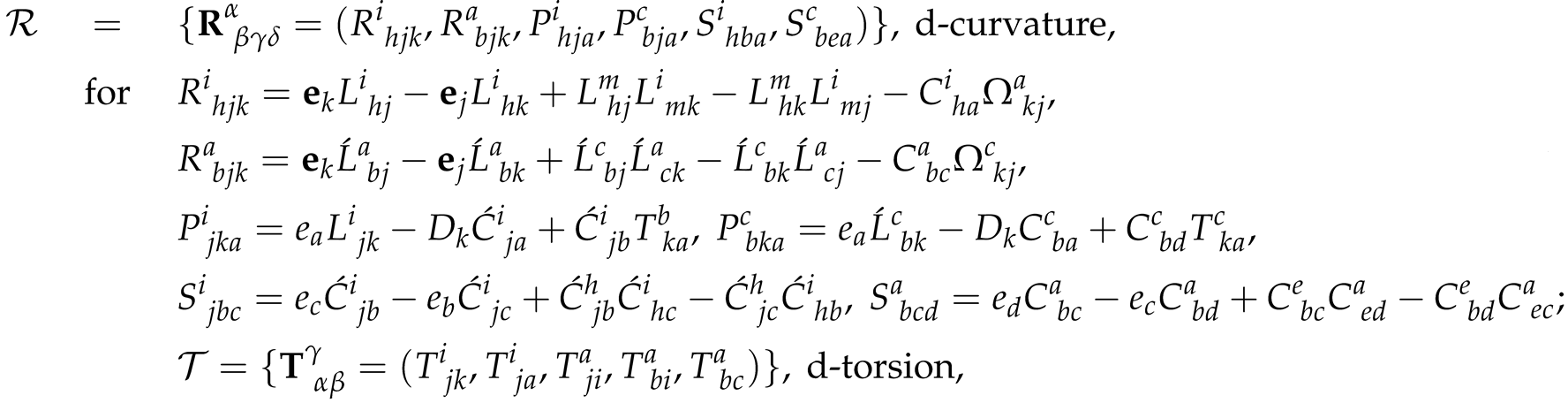
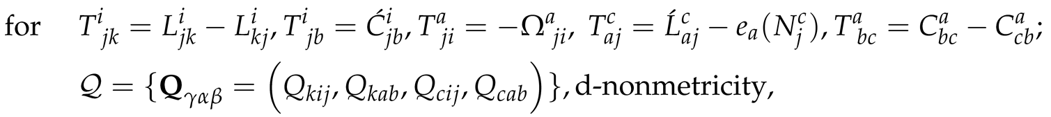
Contracting the first and forth d-indices in (40), the h-v-coefficients of the Ricci d-tensor on $\mathcal{M}$, $\mathbf{R}ic=\{{\mathbf{R}}_{⁤\beta \gamma }:={\mathbf{R}}_{⁤\beta \gamma \alpha }^{\alpha }\},$ split into four groups of coefficients,

$${\mathbf{R}}_{\alpha \beta }=\{R_{ij}:=R_{⁤ijk}^k,⁤R_{ia}:=-R_{⁤ika}^k,⁤R_{ai}:=R_{⁤aib}^b,⁤R_{ab}:=R_{⁤abc}^c\}.$$

(43)

Using the inverse d-tensor of a d-metric (15), we can compute the scalar curvature ${⁤}^{sc}R$ of $⁤\mathbf{D}$ is by definition

$$Rsc:={\mathbf{g}}^{\alpha \beta }{\mathbf{R}}_{⁤\alpha \beta }=g^{ij}{R}_{ij}+g^{ab}{R}_{ab}.$$

(44)

On a phase space ${⁤}^{|}\mathcal{M}$ with momentum variables, the formulas (40), (41) and (42) can be written for respective labels " ${⁤}^{|}$". For instance, the analogs of formulas (43) and (44) can be written in the form:

$$\begin{array}{ccc}\hfill {⁤}^{|}{\mathbf{R}}_{\alpha \beta }& =& \{{⁤}^{|}{R}_{ij}:={⁤}^{|}{R}_{⁤ijk}^k,{⁤}^{|}{R}_i^{⁤a}:=-{⁤}^{|}{R}_{⁤ik}^{k⁤a},{⁤}^{|}{R}_{⁤i}^a:={⁤}^{|}{R}_{b⁤i}^{⁤a⁤b},{⁤}^{|}{R}^{ab}:={⁤}^{|}{R}_{⁤c⁤⁤c}^{⁤ab}\}⁤\mathrm{and}⁤\hfill \\ \hfill {⁤}^{|}Rsc& =& {⁤}^{|}{\mathbf{g}}^{\alpha \beta }{⁤}^{⁤}{\mathbf{R}}_{⁤\alpha \beta }={⁤}^{|}{g}^{ij}{⁤}^{|}{R}_{ij}+{⁤}^{|}{g}_{ab}{⁤}^{|}{R}^{ab}.\hfill \end{array}$$

(45)

The formulas (40)–(45) can be written also with dyadic coefficients for any type of linear connections and d-/ s-connections (38) or (39). For canonical s-variables, such details are provided in [17,18,26].

Let us consider an important example for the canonical d-connection $\widehat{\mathbf{D}}=\{{\widehat{\Gamma }}_{⁤\alpha \beta }^{\gamma }=({\widehat{L}}_{jk}^i,{\widehat{L}}_{bk}^a,{\widehat{C}}_{jc}^i,{\widehat{C}}_{bc}^a)\}$ defined by N-adapted coefficients

$$\begin{array}{ccc}\hfill {\widehat{L}}_{jk}^i& =& {\displaystyle \frac{1}{2}}{g}^{ir}({\mathbf{e}}_k{g}_{jr}+{\mathbf{e}}_j{g}_{kr}-{\mathbf{e}}_r{g}_{jk}),\hfill \\ \hfill {\widehat{L}}_{bk}^a& =& e_b\left(N_k^a\right)+{\displaystyle \frac{1}{2}}{g}^{ac}({\mathbf{e}}_k{g}_{bc}-g_{dc}⁤e_b{N}_k^d-g_{db}⁤e_c{N}_k^d),\hfill \\ \hfill {\widehat{C}}_{jc}^i& =& {\displaystyle \frac{1}{2}}{g}^{ik}{e}_c{g}_{jk},⁤{\widehat{C}}_{bc}^a={\displaystyle \frac{1}{2}}{g}^{ad}(e_c{g}_{bd}+e_b{g}_{cd}-e_d{g}_{bc}).\hfill \end{array}$$

(46)

Such coefficients are computed for a general d–metric $\mathbf{g}=[g_{ij},g_{ab}]$ (15) with respect to N–adapted frames. Such coefficients are different from those of the LC-connection $\nabla =\left\{{\Gamma }_{⁤\alpha \beta }^{\gamma }\right\}$ computed with respect to the same system of reference. The N-adapted coefficients of the canonical distortion d-tensor in (38) can be computed as $\widehat{\mathbf{Z}}=\{{\widehat{\mathbf{Z}}}_{⁤\alpha \beta }^{\gamma }={\widehat{\Gamma }}_{⁤\alpha \beta }^{\gamma }-{\Gamma }_{⁤\alpha \beta }^{\gamma }\}.$ Introducing ${\widehat{\Gamma }}_{⁤\alpha \beta }^{\gamma }$ (46) into (40)–(44) (instead of the coefficients of a general d-connection ${\Gamma }_{⁤\alpha \beta }^{\gamma })$, we can compute the N-adapted coefficients of canonical fundamental d–objects. Such coefficients are labelled, for instance, as $\widehat{\mathcal{R}}=\{{\widehat{\mathbf{R}}}_{⁤\beta \gamma \delta }^{\alpha }=({\widehat{R}}_{⁤hjk}^i,{\widehat{R}}_{⁤bjk}^a,...)\},⁤\widehat{\mathcal{T}}=\{{\widehat{\mathbf{T}}}_{⁤\alpha \beta }^{\gamma }=({\widehat{T}}_{⁤jk}^i,{\widehat{T}}_{⁤ja}^i,...)\},$ for $\widehat{\mathcal{Q}}=\{{\widehat{\mathbf{Q}}}_{\gamma \alpha \beta }=({\widehat{Q}}_{kij}=0,{\widehat{Q}}_{kab}=0)=0,$ and similarly for ${\widehat{\mathbf{R}}}_{\alpha \beta }=\{{\widehat{R}}_{ij}:={\widehat{R}}_{⁤ijk}^k,⁤...\}$ and $\widehat{R}sc:={\mathbf{g}}^{\alpha \beta }{\widehat{\mathbf{R}}}_{⁤\alpha \beta }=g^{ij}{\widehat{R}}_{ij}+g^{ab}{\widehat{R}}_{ab}.$ Such formulas (in general, with additional nonholonomic dyadic splitting) will be used in Section 4 to prove important general decoupling and integration properties of FLH and geometric flow modified Einstein equations.

2.3. Metric and Nonmetric FLH-Deformed Einstein Equations

Finsler-like gravity theories can be formulated for two classes of d-connection structures: metric-compatible d-connections (for instance, using the Cartan or the canonical ones) or noncompatible, for instance, using the Chern or Berwald d-connections. Many variants of modified gravitational field equations were postulated by different authors as we discussed in paragraphs 3-7] of Section 1. In our approach, we argue that all FLH theories can be elaborated in a unified form as nonholonomic metric-affine theories constructed on but on relativistic phase spaces $\mathcal{M}$ and ${⁤}^{|}\mathcal{M}$ as in [13,14,16,17,18,19,26]. Explicit cases of physically important systems of nonlinear PDEs for FLH MGTs and certain classes of solutions can be distinguished by respective types of distortions, generating functions and effective sources, as we motivated in detail in [37,107,161] (see proofs in the next section).

2.3.1. Canonical Nonholonomic Metric Affine Structures in FLH Gravity

Any geometric and gravity model for nonholonomic metric-affine generalizations of FLH theories can be formulated in N-adapted form using the geometric objects (36) and (37) and respective fundamental geometric d-objects (40) - (44). The formulations in canonical nonholonomic variables (with hat-symbols) are important for decoupling and integrating corresponding modified gravitational and geometric flow equations using the AFCDM.

In metric compatible form, we shall work with the canonical d-connection $\widehat{\mathbf{D}}=\left\{{\widehat{\Gamma }}_{\beta \gamma }^{\sigma }\right\}$ (46) with the nonholonomically induced d-torsion (it can be considered as an auxiliary one to other types of torsion and nonmetricity structures on $\mathcal{M}$):

$$\widehat{\mathcal{T}}=\{{\widehat{\mathbf{T}}}_{\beta \gamma }^{\alpha }={\widehat{\Gamma }}_{\beta \gamma }^{\sigma }-{\widehat{\Gamma }}_{\gamma \beta }^{\sigma }+w_{\beta \gamma }^{\sigma }\}.$$

This canonical d-torsion which is completely determined by the coefficients of $⁤\mathbf{g}$ and $\mathbf{N}$ and anholonomy coefficients $w_{\beta \gamma }^{\sigma }$ (for Cartan-Finsler configurations, see (12)). The contortion s-tensor is defined

$$⁤{\widehat{\mathbf{K}}}_{\beta \gamma \sigma }={\widehat{\mathbf{T}}}_{\beta \gamma \sigma }+{\widehat{\mathbf{T}}}_{\gamma \sigma \beta }+{\widehat{\mathbf{T}}}_{\sigma \gamma \beta }.$$

(47)

Such values with "hats" are induced by an N-connection structure and written in N-adapted forms.8

Using the canonical distortion relations (38) can be redefined in the form

$$\mathbf{D}=\nabla +\mathbf{L}=\widehat{\mathbf{D}}+\widehat{\mathbf{L}},⁤\mathrm{where}⁤\widehat{\mathbf{L}}=\mathbf{L}-\widehat{\mathbf{Z}},$$

(48)

for an additional disformation d-tensor $\mathbf{L}=\{{\mathbf{L}}_{⁤\beta \lambda }^{\alpha }={\displaystyle \frac{1}{2}}({\mathbf{Q}}_{⁤\beta \lambda }^{\alpha }-{\mathbf{Q}}_{⁤\beta ⁤\lambda }^{⁤\alpha }-{\mathbf{Q}}_{⁤\lambda ⁤\beta }^{⁤\alpha })\},$ with ${\mathbf{Q}}_{\alpha \beta \lambda }:={\mathbf{D}}_{\alpha }{\mathbf{g}}_{\beta \lambda },$ for ${\widehat{\mathbf{Q}}}_{\alpha \beta \lambda }={\widehat{\mathbf{D}}}_{\alpha }{\mathbf{g}}_{\beta \lambda }=0.$ For nonmetric geometric constructions with disformations (48), we can use respective nonmetricity d-vectors and vectors:

$${\mathbf{Q}}_{\alpha }={\mathbf{g}}^{\beta \lambda }{\mathbf{Q}}_{\alpha \beta \lambda }={\mathbf{Q}}_{\alpha ⁤\lambda }^{⁤\lambda },{⁤}^{⊺}{\mathbf{Q}}_{\beta }={\mathbf{g}}^{\alpha \lambda }{\mathbf{Q}}_{\alpha \beta \lambda }={\mathbf{Q}}_{\alpha \beta }^{⁤\alpha }.$$

In our works, we shall use also such geometric d-objects: the nonmetricity conjugate d-tensor and tensor,

$${\widehat{\mathbf{P}}}_{⁤⁤\alpha \beta }^{\gamma }={\displaystyle \frac{1}{4}}(-2{\widehat{\mathbf{L}}}_{⁤\alpha \beta }^{\gamma }+{\mathbf{Q}}^{\gamma }{\mathbf{g}}_{\alpha \beta }-{⁤}^{⊺}{\mathbf{Q}}^{\gamma }{\mathbf{g}}_{\alpha \beta }-{\displaystyle \frac{1}{2}}{\delta }_{\alpha }^{\gamma }{\mathbf{Q}}_{\beta }-{\displaystyle \frac{1}{2}}{\delta }_{\beta }^{\gamma }{\mathbf{Q}}_{\alpha }),$$

(49)

and the nonmetricity scalar for respective d-connections and LC-connection,

$$\widehat{\mathbf{Q}}=-Q_{\alpha \beta \lambda }{\widehat{\mathbf{P}}}^{\alpha \beta \lambda },Q=-Q_{\alpha \beta \lambda }{\mathbf{P}}^{\alpha \beta \lambda }⁤\mathrm{and}⁤Q=-Q_{\alpha \beta \lambda }{P}^{\alpha \beta \lambda }.$$

(50)

Considering distortion relations (38) and (48) relating certain $\nabla =\left\{{\breve{\Gamma }}_{⁤\beta \gamma }^{\alpha }\left(u\right)\right\},$ $\mathbf{D}=\left\{{\Gamma }_{⁤\alpha \beta }^{\gamma }\right\},\widehat{\mathbf{D}}=\left\{{\Gamma }_{⁤\alpha \beta }^{\gamma }\right\}$ and $D=\left\{{\Gamma }_{⁤\alpha \beta }^{\gamma }\right\},$ we can compute corresponding distortion relations for fundamental d-tensors (40)–(45). For convenience, we provide here respective parameterizations for distortions of the Ricci d-tensor and respective Ricci scalars:

$$\begin{array}{cc}\hfill \mathbf{R}ic& =\breve{R}ic+\breve{Z}ic=\widehat{\mathbf{R}}ic+\widehat{\mathbf{Z}}ic,⁤\mathrm{for}⁤\mathrm{respective}⁤\mathrm{coefficients}⁤\hfill \\ \hfill ⁤& \mathbf{R}ic=\{{\mathbf{R}}_{\beta \gamma }={\mathbf{R}}_{⁤\beta \gamma \alpha }^{\alpha }\};\breve{R}ic=\{{\breve{R}}_{\beta \gamma }={\breve{R}}_{⁤\beta \gamma \alpha }^{\alpha }\},\breve{Z}ic=\{{\breve{Z}}_{\beta \gamma }={\breve{Z}}_{⁤\beta \gamma \alpha }^{\alpha }\};\hfill \\ \hfill ⁤& \widehat{\mathbf{R}}ic=\{{\widehat{\mathbf{R}}}_{\beta \gamma }={\widehat{\mathbf{R}}}_{⁤\beta \gamma \alpha }^{\alpha }\},\widehat{\mathbf{Z}}ic=\{{\widehat{\mathbf{Z}}}_{\beta \gamma }:={\widehat{\mathbf{Z}}}_{⁤\beta \gamma \alpha }^{\alpha }\};⁤\mathrm{and}⁤\hfill \\ \hfill \mathbf{R}sc& ={\mathbf{g}}^{\alpha \beta }{\mathbf{R}}_{⁤\alpha \beta }=\breve{R}sc+\breve{Z}sc=\widehat{\mathbf{R}}sc+\widehat{\mathbf{Z}}sc,\mathrm{where}⁤\hfill \\ \hfill ⁤& \breve{R}sc=g^{\beta \gamma }{\breve{R}}_{\beta \gamma },\breve{Z}sc=g^{\beta \gamma }{\breve{Z}}_{\beta \gamma };\widehat{\mathbf{R}}sc={\mathbf{g}}^{\alpha \beta }{\widehat{\mathbf{R}}}_{\alpha \beta },\widehat{\mathbf{Z}}sc={\mathbf{g}}^{\alpha \beta }{\widehat{\mathbf{Z}}}_{\alpha \beta }.\hfill \end{array}$$

(51)

Above geometric d-objects and objects can be used for elaborating and analyzing physical properties of various models of nonmetric geometric flows and MGTs. The motivation and priority of the canonical "hat" variables is that they allow to decouple and integrate in certain general off-diagonal forms corresponding physically important systems of nonlinear PDEs. The Greeck indices in (51) run values $\alpha ,\beta ,...=1,2,....,8.$ For dyadic decompositions, $\alpha ,\beta ,...\to {\alpha }_s,{\beta }_s,...⁤$for $s=1,2,3,4,$ etc.

2.3.2. FL Deformed Nonmetric f(Q) Gravity and Modified Einstein Equations

We can formulate on $\mathcal{M}$ a model of nonmetric Finsler-Lagrange gravity using a gravitational Lagrange density ${⁤}^g\widehat{\mathcal{L}}={\displaystyle \frac{1}{2\kappa }}\widehat{f}\left(\widehat{\mathbf{Q}}\right),$ with $\widehat{\mathbf{Q}}$ defined by formulas (50), and for the matter fields ${⁤}^m\widehat{\mathcal{L}}$ defined in "hat" variables. The total relativistic phase space action is postulated in the form:

$$\widehat{\mathcal{S}}=\int \sqrt{|{\mathbf{g}}_{\alpha \beta }|}{\delta }^{8}u({⁤}^g\widehat{\mathcal{L}}+{⁤}^m\widehat{\mathcal{L}}).$$

(52)

In this formula, hat-labels state that all Lagrange densities and geometric objects are written in nonholonomic dyadic form, with boldface indices; using $\widehat{\mathbf{D}}$ and disformations (48) and the measure $\sqrt{|{\mathbf{g}}_{\alpha \beta }|}{\delta }^{8}u,$ for ${\delta }^{8}u=d{u}^{1}d{u}^2\delta u^3\delta u^4\delta u^5\delta u^6\delta u^7\delta u^8$ with $\delta u^{a_s}={\mathbf{e}}^{a_s}$ (for $s=2,3,4$) as in formulas (18) and (19) but considered with velocity type variables.

In N-adapted variational form (see similar 4-d and 8-d constructions in [37,107,161]), or applying "pure" nonholonomic geometric methods as in [2], we can derive such nonmetric gravitational field equations:

$$\begin{array}{cc}\hfill {\displaystyle \frac{2}{\sqrt{\left|\mathbf{g}\right|}}}{\widehat{\mathbf{D}}}_{\gamma }\left(\sqrt{\left|\mathbf{g}\right|}\widehat{f_Q}{\widehat{\mathbf{P}}}_{⁤⁤\alpha \beta }^{\gamma }\right)+{\displaystyle \frac{1}{2}}\widehat{f}{\mathbf{g}}_{\alpha \beta }+\widehat{f_Q}({\widehat{\mathbf{P}}}_{\beta \mu \nu }{\mathbf{Q}}_{\alpha }^{⁤\mu \nu }-2{\widehat{\mathbf{P}}}_{\alpha \mu \nu }{\mathbf{Q}}_{⁤\beta }^{\mu \nu })& =\kappa {\widehat{\mathbf{T}}}_{\alpha \beta }\hfill \end{array}$$

(53)

$$\begin{array}{cc}\hfill ⁤\mathrm{and}⁤{\widehat{\mathbf{D}}}_{\alpha }{\widehat{\mathbf{D}}}_{\beta }\left(\sqrt{\left|\mathbf{g}\right|}\widehat{f_Q}{\widehat{\mathbf{P}}}_{⁤⁤\gamma }^{\alpha \beta }\right)& =0.\hfill \end{array}$$

(54)

In these formulas, for $\widehat{f_Q}:=\partial \widehat{f}/\partial \widehat{Q};$ with ${\widehat{\mathbf{P}}}_{⁤⁤\alpha \beta }^{\gamma }$ and ${\mathbf{Q}}_{⁤⁤\alpha \beta }^{\gamma }$ defined as in formulas (49) and (50); the energy-momentum d-tensor ${\widehat{\mathbf{T}}}_{\alpha \beta }$ is defined by N-adapted variations for ${⁤}^m\widehat{\mathcal{L}}$ on the d-metric; and all equations being written for N-elongated frames.

Using distortion relations (51), we can write the system (53) in a form provided in [168] for the Einstein tensor, $\breve{E}:=\breve{R}ic-{\displaystyle \frac{1}{2}}g\breve{R}sc$, computed for ∇ on 4-d pseudo-Riemannian manifolds, and nonmetric generalizations, with applications in DE physics [168,169].9 Such effective gravitational field equations can be generalized to 8-d phase spaces $\mathcal{M}$ in the form

$$\begin{array}{cc}\hfill {\breve{E}}_{\alpha \beta }& ={\displaystyle \frac{\kappa }{f_Q}}{⁤}^m{T}_{\alpha \beta }+{⁤}^Q{T}_{\alpha \beta }+{⁤}^z{T}_{\alpha \beta }=\kappa {\breve{T}}_{\alpha \beta },⁤\mathrm{or}⁤\hfill \end{array}$$

(55)

$$\begin{array}{cc}\hfill {\breve{R}}_{\alpha \beta }& ={\breve{{\rm Y}}}_{\alpha \beta },⁤\mathrm{where}⁤{\breve{{\rm Y}}}_{\alpha \beta }=\kappa ({\breve{T}}_{\alpha \beta }-{\displaystyle \frac{1}{2}}{g}_{\alpha \beta }\breve{T}),⁤\mathrm{for}⁤\breve{T}=g^{\alpha \beta }{\breve{T}}_{\alpha \beta },\hfill \end{array}$$

(56)

$$\begin{array}{cc}\hfill {⁤}^Q{T}_{\alpha \beta }& ={\displaystyle \frac{1}{2}}{g}_{\alpha \beta }({\displaystyle \frac{f}{f_Q}}-Q)+2{\displaystyle \frac{f_{QQ}}{f_Q}}{\nabla }_{\gamma }\left(Q{P}_{⁤⁤\alpha \beta }^{\gamma }\right),\hfill \end{array}$$

(57)

$$\begin{array}{cc}\hfill {⁤}^m{T}_{\alpha \beta }& =-{\displaystyle \frac{2}{\sqrt{\left|g\right|}}}{\displaystyle \frac{\delta \left(\sqrt{\left|g\right|}{⁤}^m\mathcal{L}\right)}{\delta g^{\alpha \beta }}}={⁤}^m\mathcal{L}{g}_{\alpha \beta }+2{\displaystyle \frac{\delta \left({⁤}^m\mathcal{L}\right)}{\delta g^{\alpha \beta }}}\hfill \end{array}$$

(58)

$$\begin{array}{cc}\hfill {⁤}^z{T}_{\alpha \beta }& =⁤[\mathrm{computed}⁤\mathrm{by}⁤\mathrm{respective}⁤\mathrm{distortion}⁤\mathrm{relations}]⁤\left(51\right).\hfill \end{array}$$

(59)

The formula (58) holds if ${⁤}^m\mathcal{L}$ does not depend in explicit form on ${\Gamma }_{⁤\alpha \beta }^{\gamma }$ (it has to be modified, for instance, for spinor fields). The nonmetric modifications of GR (with trivial extensions on velocity variables) are encoded into the effective energy-momentum tensor ${⁤}^Q{T}_{\alpha \beta }$ (57).

FL configurations can be modeled by systems of nonlinear PDEs (53), or (55), or (56) if we prescribe "tilde" N-connection and d-metric structures of type (8) and (13) for some geometric data $(\tilde{L},⁤⁤\tilde{\mathbf{N}};{\tilde{\mathbf{e}}}_{\alpha },{\tilde{\mathbf{e}}}^{\alpha };{\tilde{g}}_{jk},{\tilde{g}}^{jk}).$ Such geometric data can be subjected to general frame transforms with re-definition of frame structure and distortions of d-connections (51), for instance, choosing the variants

$$\begin{array}{ccc}\hfill {⁤}^L\widehat{\mathbf{D}}& =& {⁤}^L\nabla +{⁤}^L\widehat{\mathbf{Z}},{⁤}^L\tilde{\mathbf{D}}={⁤}^L\nabla +{⁤}^L\tilde{\mathbf{Z}},⁤\mathrm{and}⁤{⁤}^L\widehat{\mathbf{D}}={⁤}^L\mathbf{D}+{⁤}^L\mathbf{Z},⁤\mathrm{determined}⁤\mathrm{by}⁤({⁤}^L\mathbf{g},{⁤}^L\mathbf{N});\hfill \\ \hfill {⁤}_s\widehat{\mathbf{D}}& =& \tilde{\mathbf{D}}+{⁤}_s\mathbf{Z},{⁤}_s^L\widehat{\mathbf{D}}={⁤}^L\mathbf{D}+{⁤}_s^L\mathbf{Z},⁤\mathrm{determined}⁤\mathrm{by}⁤({⁤}_s\mathbf{g}\simeq {⁤}^L\mathbf{g},{⁤}_{\mathbf{s}}\mathbf{N}\simeq {⁤}^L\mathbf{N}),\hfill \end{array}$$

The nonholonomic distorted data $({⁤}^L\mathbf{N};{⁤}^L{\mathbf{e}}_{{\alpha }_s},{⁤}^L{\mathbf{e}}^{{\alpha }_s};{⁤}^L{\mathbf{g}}_{{\alpha }_s{\beta }_s},{⁤}_s^L\widehat{\mathbf{D}}),$ when a L-label is kept if $\tilde{L}\to L$ for some general frame/coordinate frame transforms on $\mathcal{M}$, can be used for applying the AFCDM.

2.3.3. FH Deformed Nonmetric f(${⁤}^{|}$Q) Gravity and Modified Einstein Equations

In similar forms, we can define nonmetric gravity models on dual phase space ${⁤}^{|}\mathcal{M}$ enabled with Hamilton generating functions. Using a gravitational Lagrange density ${⁤}_{|}^g\widehat{\mathcal{L}}={\displaystyle \frac{1}{2\kappa }}{⁤}^{|}\widehat{f}\left({⁤}^{|}\widehat{\mathbf{Q}}\right),$ with ${⁤}^{|}\widehat{\mathbf{Q}}$ defined by formulas which are conventionally dual to (50) and for the matter fields ${⁤}_{|}^m\widehat{\mathcal{L}}$ defined in "hat" variables involving Legendre transforms and respective co-fiber coordinates. The total relativistic phase space action is postulated (if necessary, related to (52)) as

$${⁤}^{|}\widehat{\mathcal{S}}=\int \sqrt{|{⁤}^{|}{\mathbf{g}}_{\alpha \beta }|}{\delta }^8{⁤}^{|}u({⁤}_{{⁤}^{|}}^g\widehat{\mathcal{L}}+{⁤}_{{⁤}^{|}}^m\widehat{\mathcal{L}}).$$

In this formula, hat-labels state that all Lagrange densities and geometric objects are written in nonholonomic dyadic form, with boldface indices; using $\widehat{\mathbf{D}}$ and disformations (48) and the measure $\sqrt{|{⁤}^{|}{\mathbf{g}}_{\alpha \beta }|}{\delta }^8{⁤}^{⁤}u,$ for ${\delta }^8{⁤}^{|}u=d{u}^{1}d{u}^2\delta u^3\delta u^4\delta {⁤}^{|}{u}^5\delta {⁤}^{⁤}{u}^6\delta {⁤}^{|}{u}^7\delta {⁤}^{|}{u}^8$ with $\delta {⁤}^{|}{u}^{a_s}={⁤}^{|}{\mathbf{e}}^{a_s},$ (for $s=2,3,4$) as in (18) and (19) using momentum type variables ${⁤}^{|}{u}^{a_s}=(p_{a_3},p_{a_4}),$ for $s=3,4.$ We can consider three variants to derive respective nonmetric phase space gravitational equations: 1) to perform a N-adapted variational form for ${⁤}^{|}\widehat{\mathcal{S}};$ 2) or to apply geometric methods as in [2]; or 3) to take dual formulas for (53) and (54). We obtain such nonmetric gravitational field equations on ${⁤}^{|}\mathcal{M}$:

$$\begin{array}{cc}\hfill {\displaystyle \frac{2}{\sqrt{|{⁤}^{|}\mathbf{g}|}}}{⁤}^{|}{\widehat{\mathbf{D}}}_{\gamma }\left(\sqrt{|{⁤}^{|}\mathbf{g}|}{⁤}^{|}\widehat{f_Q}{⁤}^{|}{\widehat{\mathbf{P}}}_{⁤⁤\alpha \beta }^{\gamma }\right)+{\displaystyle \frac{1}{2}}{⁤}^{|}\widehat{f}{⁤}^{|}{\mathbf{g}}_{\alpha \beta }+{⁤}^{|}\widehat{f_Q}({⁤}^{|}{\widehat{\mathbf{P}}}_{\beta \mu \nu }{⁤}^{|}{\mathbf{Q}}_{\alpha }^{⁤\mu \nu }-2{⁤}^{|}{\widehat{\mathbf{P}}}_{\alpha \mu \nu }{⁤}^{|}{\mathbf{Q}}_{⁤\beta }^{\mu \nu })& =\kappa {⁤}^{|}{\widehat{\mathbf{T}}}_{\alpha \beta }\hfill \end{array}$$

(60)

$$\begin{array}{cc}\hfill ⁤\mathrm{and}⁤{⁤}^{|}{\widehat{\mathbf{D}}}_{\alpha }{⁤}^{|}{\widehat{\mathbf{D}}}_{\beta }\left(\sqrt{|{⁤}^{|}\mathbf{g}|}{⁤}^{|}\widehat{f_Q}{⁤}^{|}{\widehat{\mathbf{P}}}_{⁤⁤\gamma }^{\alpha \beta }\right)& =0.\hfill \end{array}$$

(61)

In these formulas, for ${⁤}^{|}\widehat{f_Q}:=\partial {⁤}^{|}\widehat{f}/\partial {⁤}^{|}\widehat{Q};$ with ${⁤}^{|}{\widehat{\mathbf{P}}}_{⁤⁤\alpha \beta }^{\gamma }$ and ${⁤}^{|}{\mathbf{Q}}_{⁤⁤\alpha \beta }^{\gamma }$ defined in dual form to formulas (49) and (50); the energy-momentum d-tensor ${⁤}^{|}{\widehat{\mathbf{T}}}_{\alpha \beta }$ is defined by N-adapted variations for ${⁤}_{⁤}^m\widehat{\mathcal{L}}$ on the d-metric; and all equations involve N-elongated frames.

FH configurations are modeled in canonical form by systems of nonlinear PDEs (60) and (61) if we prescribe "tilde" N-connection and d-metric structures of type (8), (37) and (14) for the nonholonomic geometric data $(\tilde{H},{⁤}^{|}\tilde{\mathbf{N}};{⁤}^{|}{\tilde{\mathbf{e}}}_{\alpha },{⁤}^{|}{\tilde{\mathbf{e}}}^{\alpha };⁤{⁤}^{|}{\tilde{g}}^{ab},⁤{⁤}^{|}{\tilde{g}}_{ab}).$ Such geometric data can be subjected to general frame transforms with re-definition of frame structure and distortions of d-connections (39), for instance, choosing the variants

$$\begin{array}{ccc}\hfill {⁤}_{|}^H\widehat{\mathbf{D}}& =& {⁤}_{|}^H\nabla +{⁤}_{|}^H\widehat{\mathbf{Z}},{⁤}_{|}^H\tilde{\mathbf{D}}={⁤}_{|}^H\nabla +{⁤}_{|}^H\tilde{\mathbf{Z}},⁤\mathrm{and}⁤{⁤}_{|}^H\widehat{\mathbf{D}}={⁤}_{|}^H\mathbf{D}+{⁤}_{|}^H\mathbf{Z},⁤\mathrm{determined}⁤\mathrm{by}⁤({⁤}_{|}^H\mathbf{g},{⁤}_{|}^H\mathbf{N});\hfill \\ \hfill {⁤}_s^{|}\widehat{\mathbf{D}}& =& {⁤}^{|}\tilde{\mathbf{D}}+{⁤}_s^{|}\mathbf{Z},{⁤}_s^H\widehat{\mathbf{D}}={⁤}_{|}^H\mathbf{D}+{⁤}_s^H\mathbf{Z},⁤\mathrm{determined}⁤\mathrm{by}⁤({⁤}_s^{|}\mathbf{g}\simeq {⁤}_{|}^H\mathbf{g},{⁤}_s^{|}\mathbf{N}\simeq {⁤}_{|}^H\mathbf{N}),\hfill \end{array}$$

The nonholonomic distorted data $({⁤}_{|}^H\mathbf{N};{⁤}_{|}^H{\mathbf{e}}_{{\alpha }_s},{⁤}_{|}^H{\mathbf{e}}^{{\alpha }_s};{⁤}_{|}^H{\mathbf{g}}_{{\alpha }_s{\beta }_s},{⁤}_{s|}^H\widehat{\mathbf{D}}),$ when a H-label is kept if $\tilde{H}\to H$ for some general frame/coordinate frame transforms on ${⁤}^{|}\mathcal{M}$, can be used for applying the AFCDM.

In general, Hamiltonian mechanics is not equivalent to Lagrangian mechanics. For instance, in the first case, we consider symplectomorphisms as specific symmetries related to almost symplectic and almost complex structures studied in [17,19,50,51,52,53,107,167]. In this work, we do not study Hamilton and almost symplectic models of (dual) Finsler-Lagrange geometry and respective nonholonomic d-connection structures. The system of nonlinear PDEs (60) can be written in equivalent form by using the LC-connection ${⁤}^{|}{\nabla }_{\gamma }$ with respective dual equations to (55), or (59). Such equations can be reduced in nonholonomic and parametric form to the Einstein equations in GR if ${⁤}^{|}{\nabla }_{\gamma }\to ⁤({\nabla }_{i_1},{\nabla }_{a_2})$ and the d-metric structure is transformed into (24).

2.3.4. Canonical Integrable Nonmetric FLH Deformed Gravitational Phase Space Equations

To decouple and solve in certain general off-diagonal forms systems of nonlinear PDEs (53) and (60) is not possible because of various nonholonomic constraints and coupling conditions like (54) or, respectively, (61). We have to re-define such FLH-modified gravitational field equations in corresponding nonholonomic s-variables which allows us to apply the AFCDM. Let us explain how such nonholonomic transforms can be performed in explicit form:

On $\mathcal{M}$, we can use distortions (51) and write (55) in the form

$$\begin{array}{cc}\hfill {\widehat{\mathbf{R}}}_{\alpha \beta }& ={⁤}_Q{\widehat{⁤}}_{\alpha \beta },⁤\mathrm{for}⁤\hfill \end{array}$$

(62)

$$\begin{array}{cc}\hfill {⁤}_Q{\widehat{⁤}}_{\alpha \beta }& ={⁤}^e{\widehat{\mathbf{Y}}}_{\alpha \beta }+{⁤}^m{\widehat{\mathbf{Y}}}_{\alpha \beta }.\hfill \end{array}$$

(63)

The source ${⁤}_Q{\widehat{⁤}}_{\alpha \beta }$ (63) for (62) is defined by two d-tensors: the first one with effective source (e), ${⁤}^e{\widehat{\mathbf{Y}}}_{\alpha \beta }=\breve{Z}i{c}_{\alpha \beta }-\widehat{\mathbf{Z}}i{c}_{\alpha \beta }$, is of geometric distorting nature, which can be computed in explicit form using (51). The second one is the energy-momentum d-tensor ${⁤}^m{\widehat{\mathbf{Y}}}_{\alpha \beta }$ of the matter fields ${\breve{{\rm Y}}}_{\alpha \beta }$ encoding also contributions of the nonmetricity scalar $\widehat{\mathbf{Q}}$ and d-tensor ${\widehat{\mathbf{P}}}_{⁤⁤\alpha \beta }^{\gamma }$ defined respectively by formulas (50), (49) and (50). For the effective and matter field sources in above system of nonlinear PDEs, we can consider any type nonholonomic transforms of d-metrics (${\mathbf{g}}_{\alpha \beta }=e_{⁤\alpha }^{\underline{\alpha }}⁤e_{⁤\beta }^{\underline{\beta }}⁤g_{\underline{\alpha }\underline{\beta }}$ or s-adapted ones,$⁤{\mathbf{g}}_{{\alpha }_s{\beta }_s}=e_{⁤{\alpha }_s}^{\underline{\alpha }}⁤e_{⁤{\beta }_s}^{\underline{\beta }}⁤g_{\underline{\alpha }\underline{\beta }})$ and respective re-distributions of distortions, when the s-adapted form of sources (63) is parameterized

$${⁤}_Q{\widehat{⁤}}_{⁤⁤{\beta }_s}^{{\alpha }_s}=[{⁤}_1{\rm Y}\left(x^{k_1}\right){\delta }_{⁤⁤j_1}^{i_1},{⁤}_2{\rm Y}(x^{k_1},y^{c_2}){\delta }_{⁤⁤b_2}^{a_2},{⁤}_3{\rm Y}(x^{k_1},y^{c_2},v^{c_3}){\delta }_{⁤⁤b_3}^{a_3},{⁤}_4{\rm Y}(x^{k_1},y^{c_2},v^{c_3},v^{c_4}){\delta }_{⁤⁤b_4}^{a_4}],$$

(64)

where the effective sources can be parameterized in conventional oriented forms ${⁤}_s{\rm Y}(x^{k_{s-1}},v^{a_s}).$ Such s-adapted parameterizations of ${\widehat{\mathbf{R}}}_{{\alpha }_s{\beta }_s}$ and ${⁤}_Q{\widehat{⁤}}_{{\alpha }_s{\beta }_s}$ are important for explicit integrations of nonmetric FLH gravitational equations. For $\widehat{\mathbf{Q}}\to 0,$ we shall be able to generate solutions with nontrivial $\widehat{\mathcal{T}}=\left\{{\widehat{\mathbf{T}}}_{⁤\alpha \beta }^{\gamma }\right\},$ and then to extract LC-configurations ∇ (as we prove in the next section and Appendix).

We can define canonical d-equations on dual phase space ${⁤}^{|}\mathcal{M}$ encoding Hamilton generating functions and respective nonmetric distortions:

$$\begin{array}{cc}\hfill {⁤}^{|}{\widehat{\mathbf{R}}}_{\alpha \beta }& ={⁤}_Q^{|}{\widehat{⁤}}_{\alpha \beta },⁤\mathrm{for}⁤\hfill \end{array}$$

(65)

$$\begin{array}{cc}\hfill {⁤}_Q^{|}{\widehat{⁤}}_{\alpha \beta }& ={⁤}_{|}^e{\widehat{\mathbf{Y}}}_{\alpha \beta }+{⁤}_{|}^m{\widehat{\mathbf{Y}}}_{\alpha \beta },\hfill \end{array}$$

(66)

when the nonholonomic s-adapted parametrization of the sources is stated in the form

$${⁤}_Q^{|}{\widehat{⁤}}_{⁤⁤{\beta }_s}^{{\alpha }_s}=[{⁤}_1^{|}{\rm Y}\left(x^{k_1}\right){\delta }_{⁤⁤j_1}^{i_1},{⁤}_2^{|}{\rm Y}(x^{k_1},y^{c_2}){\delta }_{⁤⁤b_2}^{a_2},{⁤}_3^{|}{\rm Y}(x^{k_1},y^{c_2},p_{c_3}){\delta }_{a_3}^{⁤b_3},{⁤}_4^{|}{\rm Y}(x^{k_1},y^{c_2},p_{c_3},p_{c_4}){\delta }_{a_4}^{⁤b_4}].$$

(67)

2.3.5. Modelling, Distorting, or Extracting Gravitational Field Equations in GR and FLH MGTs

The systems of FLH equations (62) and (65) with respective sources ${⁤}_Q{\widehat{⁤}}_{⁤⁤{\beta }_s}^{{\alpha }_s}$ (64) and ${⁤}_Q{\widehat{⁤}}_{\alpha \beta }$ (67) can be integrated in general forms as we shall prove in Section 4. In abstract geometric forms, the corresponding FLH MGTs can be stated by such data:

$$\begin{array}{ccc}\hfill (⁤\tilde{\mathcal{M}}& :& F⁤\mathrm{or}⁤L;\tilde{\mathbf{g}}\simeq {⁤}_s\tilde{\mathbf{g}},⁤\tilde{\mathbf{N}}\simeq {⁤}_s⁤\tilde{\mathbf{N}},{⁤}_s\widehat{\mathbf{D}}=\tilde{\mathbf{D}}+{⁤}_s\mathbf{Z},{⁤}_{⁤}^g\widehat{\mathcal{L}}+{⁤}_{⁤}^m\widehat{\mathcal{L}},{⁤}_Q{\widehat{⁤}}_{\alpha \beta },\widehat{\mathbf{Q}}\simeq \tilde{\mathbf{Q}}=0,\hfill \\ & & ⁤\mathrm{for}⁤\mathrm{Lagrange}⁤-⁤\mathrm{Finsler}⁤-⁤\mathrm{Cartan}⁤\mathrm{configurations});\hfill \\ \hfill (⁤{⁤}^C\mathcal{M}& :& F⁤\mathrm{or}⁤L;\mathbf{g}\simeq {⁤}_s\mathbf{g},⁤{⁤}^C\mathbf{N}\simeq {⁤}_s^C\mathbf{N},{⁤}_s^C\widehat{\mathbf{D}}={⁤}^C\mathbf{D}+{⁤}_s^C\mathbf{Z},{⁤}_{{⁤}^C}^g\widehat{\mathcal{L}}+{⁤}_{{⁤}^C}^m\widehat{\mathcal{L}},{⁤}_Q^C{\widehat{⁤}}_{\alpha \beta },{⁤}^C\widehat{\mathbf{Q}}\simeq {⁤}^C\mathbf{Q}=0,\hfill \\ & & ⁤\mathrm{for}⁤\mathrm{Lagrange}⁤-⁤\mathrm{Finsler}⁤-⁤\mathrm{Chern}⁤\mathrm{configurations});\hfill \\ \hfill ({⁤}^B\mathcal{M}& :& F⁤\mathrm{or}⁤L;\mathbf{g}\simeq {⁤}_s\mathbf{g},⁤{⁤}^B\mathbf{N}\simeq {⁤}_s^B⁤\mathbf{N},{⁤}_s^B\widehat{\mathbf{D}}={⁤}^B\mathbf{D}+{⁤}_s^B\mathbf{Z},{⁤}_{{⁤}^B}^g\widehat{\mathcal{L}}+{⁤}_{{⁤}^B}^m\widehat{\mathcal{L}},{⁤}_Q^B{\widehat{⁤}}_{\alpha \beta },{⁤}^B\widehat{\mathbf{Q}}\simeq {⁤}^B\mathbf{Q}=0,\hfill \\ & & ⁤\mathrm{for}⁤\mathrm{Lagrange}⁤-⁤\mathrm{Finsler}⁤-⁤\mathrm{Berwald}⁤\mathrm{configurations});\hfill \\ \hfill (⁤\widehat{\mathcal{M}}& :& ⁤\mathrm{we}⁤\mathrm{can}⁤\mathrm{prescribe}⁤L;\mathbf{g}\simeq {⁤}_s\mathbf{g},⁤\mathbf{N}\simeq {⁤}_s⁤\mathbf{N},{⁤}_s\widehat{\mathbf{D}}=⁤\nabla +{⁤}_s\mathbf{Z},{⁤}_{⁤}^g\widehat{\mathcal{L}}+{⁤}_{⁤}^m\widehat{\mathcal{L}},{⁤}_Q{\widehat{⁤}}_{\alpha \beta },⁤\widehat{\mathbf{Q}}=0,⁤\widehat{\mathbf{T}}\ne 0,\hfill \\ & & ⁤\mathrm{for}⁤\mathrm{phase}⁤\mathrm{space}⁤\mathrm{canonical}⁤\mathrm{configurations});\hfill \\ \hfill ({⁤}_{\nabla }⁤\widehat{\mathcal{M}}& :& \mathbf{g}\simeq {⁤}_s\mathbf{g},⁤\mathbf{N}\simeq {⁤}_s⁤\mathbf{N},{⁤}_s\widehat{\mathbf{D}}=⁤\nabla +{⁤}_s\mathbf{Z},{⁤}_{⁤}^g\widehat{\mathcal{L}}+{⁤}_{⁤}^m\widehat{\mathcal{L}},{⁤}_Q{\widehat{⁤}}_{\alpha \beta },⁤\widehat{\mathbf{Q}}=0,⁤\widehat{\mathbf{T}}=0,{\widehat{\mathbf{D}}}_{|\mathcal{T}=0}=\nabla \hfill \\ & & ⁤\mathrm{extracting}⁤\mathrm{phase}⁤\mathrm{space}⁤\mathrm{LC}-\mathrm{configurations});\hfill \\ \hfill (\mathcal{M}& :& \mathbf{g}\simeq {⁤}_s\mathbf{g},⁤\mathbf{N}\simeq {⁤}_s⁤\mathbf{N},{⁤}_s\widehat{\mathbf{D}}=⁤\mathbf{D}+{⁤}_s\mathbf{Z},{⁤}_{⁤}^g\widehat{\mathcal{L}}+{⁤}_{⁤}^m\widehat{\mathcal{L}},{⁤}_Q{\widehat{⁤}}_{\alpha \beta },⁤\widehat{\mathbf{Q}}\simeq \mathbf{Q}\ne 0,⁤\widehat{\mathbf{T}}\simeq \mathbf{T}\ne 0),\hfill \\ & & ⁤\mathrm{nonholonomic}⁤\mathrm{metric}-\mathrm{affine}⁤\mathrm{phase}⁤\mathrm{spaces};\hfill \\ \hfill ({⁤}_{\mathbf{Q}}\mathcal{M}& :& \mathbf{g}\simeq {⁤}_s\mathbf{g},⁤\mathbf{N}\simeq {⁤}_s⁤\mathbf{N},{⁤}_s\widehat{\mathbf{D}}=⁤\mathbf{D}+{⁤}_s\mathbf{Z},{⁤}_{⁤}^g\widehat{\mathcal{L}}+{⁤}_{⁤}^m\widehat{\mathcal{L}},{⁤}_Q{\widehat{⁤}}_{\alpha \beta },⁤\widehat{\mathbf{Q}}\simeq \mathbf{Q}\ne 0,⁤\widehat{\mathbf{T}}\ne 0,\mathcal{T}[\nabla ]=\mathbf{0}),\hfill \\ & & ⁤\mathrm{nonmetric}⁤\mathrm{phase}⁤\mathrm{space}⁤\widehat{f}\left(\widehat{\mathbf{Q}}\right)⁤\mathrm{gravity}⁤.\hfill \end{array}$$

(68)

In the above formulas, we use "≃" to state equivalence up to a certain frame and distortion of connections transforms.

The MGT theories defined above for $\mathcal{M}$ can be formulated in similar forms on ${⁤}^{|}\mathcal{M}$ using momentum-like variables and geometric objects and (effective) Lagrangians and sources labelled by "${⁤}^{|}$".

Let us discuss how various types of FLH theories analyzed in paragraphs 1-7] of Section 1 can be included, modelled, or generalized to MGTs on (co) tangent Lorentz bundles classified in (68):

Perhaps, the simplest analysis concerns the class of models and solutions for Finsler-Randers-Sasaki theories studied in [153,154,155,156,157] using Sasaki d-metrics of type ${\tilde{\mathbf{g}}}_{\alpha \beta }(x,y)$ (13) and (typically) certain metric compatible Finsler d-connections ${⁤}^F\mathbf{D}$. Performing respective s-adapted frame transforms with ${\mathbf{g}}_{{\alpha }_s{\beta }_s}=e_{⁤{\alpha }_s}^{\alpha }⁤e_{⁤{\beta }_s}^{\beta }⁤{\tilde{\mathbf{g}}}_{\alpha \beta }$ and distortion ${⁤}_s\widehat{\mathbf{D}}={⁤}^F\mathbf{D}+{⁤}_s^F\mathbf{X}$ and parameterizations of sources ${⁤}_Q{\widehat{⁤}}_{⁤⁤{\beta }_s}^{{\alpha }_s}$ (64) (if necessary, we consider $Q=0$), we can impose the conditions that ${\mathbf{g}}_{{\alpha }_s{\beta }_s}$ is determined by a solution of (62). For such constructions, we can embed respective Finsler-Randers configurations into more general classes of FLH theories discussed above.

Considering models on $\mathcal{M},$ with respective Sasaki d-metrics, effective sources and d-connections, we can model Barthel-Randers/ - Koropina models [137,138,139] as some sub-classes of solutions of (62). Of course, we have to adapt respectively to the N-connection structures and restrict the classes of generating and integration functions.

Then, we can model in our approach certain alternative variants and extensions of the works [125,126,127,131,134,135,136] which are not necessarily formulated on (co) tangent Lorentz bundles and may involve (nonmetric) Berwald d-connection, or metric Cartan d-connections, respective sources, etc. The main assumption for such solutions is that we do not enter into "exotic" locally anisotropic causality scenarios, but perform all constructions on $\mathcal{M}$. The N-adapted variational calculus and effective sources can be chosen as, for instance, in [125,126]. Furthermore, noholonomic s-adapted frame transforms and distortions of connections enable us to speculate on metric and nonmetric FLH theories with EYMHD configurations, which can be defined and studied if we follow only the original Pfeifer- Wohlarth particular model. The variants with modified Einstein equations (62) and (65) offer such possibilities even for some particular cases of effective sources ${⁤}_Q{\widehat{⁤}}_{⁤⁤{\beta }_s}^{{\alpha }_s}$ (64) and ${⁤}_Q{\widehat{⁤}}_{\alpha \beta }$ (67).

Finally, in this subsection, we briefly discuss how we can reproduce in a relativistic and self-consistent form the results and (numerical and graphic) methods from [145,146,147]. In those works, the lifts and deformations from a base spacetimes with extensions to certain y-variables are performed using Akbar-Zadekh constructions [140,141] or the version of Finsler modified Einstein equations from [129]. In principle, such models are incomplete and undetermined if we do not introduce Sasaki-like lifts on total spaces, and do not perform a (co) tangent Lorentz bundle formulation. We can construct arbitrary y-deformations and speculate on any types of local anisotropy and y-deformations as mentioned in 7.4] of Section 1. Nevertheless, we can consider similar models with Sasaki lifts to d-metrics, when solutions of systems (62) and (65) (for certain subclasses of generating functions and sources will reproduce BH, WH and cosmological scenarios proposed in certain phenomenological and numerical forms in the mentioned works). They consist of particular cases, or nonholonomic deformations and distortion of the d-metrics studied and reviewed in [13,17,18,148,149,150,151,152,158].

3. Metric and Nonmetric Geometric FLH-Flows and Ricci Solitons

The systems of nonlinear PDE equations (62) and (65) consist examples of associative and commutative nonholonomic Ricci solitons defined as particular cases of self-similar nonassociative geometric flows on metric compatible 8-d phase spaces in our recent works [13,17,18,158,170,171]. Such constructions of generic off-diagonal solutions encoding nonmetricity were also performed in [37,107,161]. We shall consider applications of the AFCDM and explicit 8-d examples encoding nonmetric FLH configurations in Section 4 and Section 5.

The generic off-diagonal solutions constructed and studied in various MGTs (including FLH models) are not characterized, in general, by certain hypersurface or holographic conditions. As we explained in paragraph 6.4] of Section 1, the Bekenstein–Hawking BH thermodynamic paradigm [113,114] does not apply even to off-diagonal classes of quasi-stationary and regular BH solutions in GR [20]. In the case of FLH deformations of the Einstein equations, similar issues exist and this motivates the elaboration of corresponding models of nonholonomic and Finsler-like geometric flows. The goal of this section is to formulate and study such metric and nonmetric FLH geometric flow theories and related statistical thermodynamic models as generalizations of the results and methods from a series of works on Riemannian geometric flows and various relativistic and non-Riemannian modifications [53,106,108,109,110,111,112,115,116,117,118,119].

3.1. Metric Compatible FL and FH Deformed Geometric Flows

We note that in our works on nonholonomic relativistic and/or FLH (non) metric geometric flows generalizations of the famous Poincaré–Thurston conjecture are not formulated/ proved. This is a very difficult mathematical problem which depends on the types of metric and N- and d-connection structures, i.e. can’t be formulated and proven in some general nonholonomic metric-affine forms. Nevertheless, we use the concept of W-entropy [108], which is useful for formulating statistical and geometric thermodynamic models characterizing physical properties of FLH theories and respective classes of nonholonomic geometric evolutions or dynamical equations. Corresponding thermodynamic variables involve families of distorted Ricci tensors and respective Ricci scalars defined typically by $\tau$-families of metrics $g_{\alpha \beta }\left(\tau \right):=g_{\alpha \beta }(\tau ,u^{\gamma })$ and linear connections ${\Gamma }_{⁤\alpha \beta }^{\gamma }\left(\tau \right):={\Gamma }_{⁤\alpha \beta }^{\gamma }(\tau ,u^{\gamma })$, where $\tau$ is a positive flow parameter (treated as a conventional temperature). Typically, we shall write for the geometric objects only the $\tau$-parametric dependencies if that will not result in ambiguities, for instance, ${⁤}_s\widehat{\mathbf{D}}\left(\tau \right),{⁤}^F\mathbf{D}\left(\tau \right),\tilde{\mathbf{g}}\left(\tau \right)=\left\{{\tilde{\mathbf{g}}}_{\alpha \beta }\left(\tau \right)\right\},$ etc. The priority of our nonholonomic approach is that we apply the AFCDM to decouple and solve in general off-diagonal forms respective systems of nonlinear PDEs, which define FLH geometric flow evolution models or, for fixed $\tau ={\tau }_0,$ nonholonomic Ricci soliton configurations which are equivalent to certain classes of FLH gravity theories.

3.1.1. F- and W-Functionals for FL and FH Flows

Let us consider a FL phase space $\tilde{\mathcal{M}}$ and FH phase space ${⁤}^{|}\tilde{\mathcal{M}}$ which admit respective re-definitions in canonical 4+4 or nonholonomic dyadic variables as in (68), with respective classes of nonholonomic equivalence, $\tilde{\mathcal{M}}\simeq \widehat{\mathcal{M}}\simeq {⁤}_s\widehat{\mathcal{M}}$ and ${⁤}^{|}\tilde{\mathcal{M}}\simeq {⁤}^{|}\widehat{\mathcal{M}}\simeq {⁤}_s^{|}\widehat{\mathcal{M}}$. For simplicity, in this subsection (with metric-compatible geometric constructions), we consider only "tilde" geometric objects. The models with "hat" connections can be formulated in similar forms, when the s-adapted variants result in respective FL and FH geometric flow equations, which can be integrated in general off-diagonal form (we prove it in Section 4 in certain general forms with nonmetricity).

We consider FL and FH flows on temperature like parameter $\tau$ (when $0\le \tau \le {\tau }_0$) of d-objects on, respective, $\tilde{\mathcal{M}}$ and ${⁤}^{|}\tilde{\mathcal{M}},$ by using $\tau$-flows of volume elements

$$d⁤⁤\tilde{\mathcal{V}}ol\left(\tau \right)=\sqrt{|⁤{\tilde{\mathbf{g}}}_{\alpha \beta }⁤\left(\tau \right)|}⁤{\tilde{\delta }}^8⁤u^{{\gamma }_s}\left(\tau \right)⁤\mathrm{and}⁤d⁤{⁤}^{|}\tilde{\mathcal{V}}ol\left(\tau \right)=\sqrt{|⁤{⁤}^{|}{\tilde{\mathbf{g}}}_{\alpha \beta }⁤\left(\tau \right)|}⁤{⁤}^{|}{\tilde{\delta }}^8{⁤}^{|}{u}^{{\gamma }_s}\left(\tau \right).$$

(69)

Such a value is computed using N-elongated s-differentials, for instance, ${⁤}^{|}{\tilde{\delta }}^8{⁤}^{|}{u}^{{\gamma }_s}\left(\tau \right),$ which are linear on ${⁤}^{|}{\tilde{N}}_{⁤i_s{a}_s}⁤\left(\tau \right)$ as in ${⁤}^{|}{\tilde{\mathbf{e}}}_{{\alpha }_s}\left(\tau \right),$ see formulas (19) and (18). Nonholonomic geometric flow theories can be formulated for the geometric data $[\tilde{\mathbf{g}}\left(\tau \right),\tilde{\mathbf{D}}\left(\tau \right)]$ and $[{⁤}^{|}\tilde{\mathbf{g}}\left(\tau \right),{⁤}^{|}\tilde{\mathbf{D}}\left(\tau \right)],$ when the Perelman type functionals are respectively postulated:

$$\begin{array}{ccc}\hfill ⁤\tilde{\mathcal{F}}\left(\tau \right)& =& {\int }_{⁤\tilde{\Xi }}(\tilde{\mathbf{R}}sc+|\tilde{\mathbf{D}}\tilde{f}{|}^2)e^{-⁤\tilde{f}}⁤d\tilde{\mathcal{V}}ol\left(\tau \right),\hfill \end{array}$$

(70)

$$\begin{array}{ccc}\hfill ⁤\tilde{\mathcal{W}}\left(\tau \right)& =& {\int }_{⁤\tilde{\Xi }}{\left(4\pi \tau \right)}^{-4}⁤\left[\tau \right(\tilde{\mathbf{R}}sc+|\tilde{\mathbf{D}}\tilde{f}{\left|\right)}^2+\tilde{f}-8]e^{-⁤\tilde{f}}⁤d⁤\tilde{\mathcal{V}}ol\left(\tau \right);\hfill \\ & & ⁤\mathrm{and}⁤\hfill \end{array}$$

(71)

$$\begin{array}{ccc}\hfill {⁤}^{|}\tilde{\mathcal{F}}\left(\tau \right)& =& {\int }_{{⁤}^{|}\tilde{\Xi }}({⁤}^{|}\tilde{\mathbf{R}}sc+|{⁤}^{|}\tilde{\mathbf{D}}{⁤}^{|}\tilde{f}{|}^2)e^{-{⁤}^{|}\tilde{f}}⁤d{⁤}^{|}\tilde{\mathcal{V}}ol\left(\tau \right),\hfill \\ \hfill {⁤}^{|}\tilde{\mathcal{W}}\left(\tau \right)& =& {\int }_{{⁤}^{|}\tilde{\Xi }}{\left(4\pi \tau \right)}^{-4}⁤\left[\tau \right({⁤}^{|}\tilde{\mathbf{R}}sc+|{⁤}^{|}\tilde{\mathbf{D}}{⁤}^{⁤}\tilde{f}{\left|\right)}^2+{⁤}^{|}\tilde{f}-8]e^{-⁤{⁤}^{|}\tilde{f}}⁤d{⁤}^{|}\tilde{\mathcal{V}}ol\left(\tau \right).\hfill \end{array}$$

The 8-d hypersurfrace integrals $⁤\tilde{\Xi }$ and for ${⁤}^{|}\tilde{\Xi }$, such F- and W-functionals are determined by volume elements (69). For instance, a h-c-normalizing function ${⁤}^{|}\tilde{f}(\tau ,{⁤}^{|}u)$ can be stated to satisfy the condition

$${\int }_{{⁤}^{|}\tilde{\Xi }}{⁤}^{|}\tilde{\nu }⁤⁤d{⁤}^{|}\tilde{\mathcal{V}}ol\left(\tau \right):={\int }_{t_1}^{t_2}{\int }_{{\tilde{\Xi }}_t}⁤{\int }_{{⁤}^{|}{\tilde{\Xi }}_E}{⁤}^{|}\tilde{\nu }⁤⁤d{⁤}^{|}\tilde{\mathcal{V}}ol\left(\tau \right)=1.$$

(72)

In these formulas, where the integration measures $⁤{⁤}^{|}\tilde{\nu }={\left(4\pi \tau \right)}^{-4}{e}^{-{⁤}^{|}\tilde{f}}$ are parameterized for the h- and c-components, with shell further parameterizations if necessary. For general topological considerations, such conditions may not be considered. We can also choose certain variants of $\tilde{f}$ or ${⁤}^{|}\tilde{f}$ to simplify certain formulas and computations.

The FL and FH geometric flow evolution equations are postulated in the form

$$\begin{array}{ccc}\hfill {\partial }_{\tau }{\tilde{\mathbf{g}}}_{\alpha \beta }\left(\tau \right)& =& -2{\tilde{\mathbf{R}}}_{⁤\alpha \beta }\left(\tau \right),\hfill \\ \hfill {\partial }_{\tau }\tilde{f}\left(\tau \right)& =& \tilde{\mathbf{R}}sc\left(\tau \right)-⁤\widetilde{△}\left(\tau \right)\tilde{f}\left(\tau \right)+{\left(\tilde{\mathbf{D}}\left(\tau \right)\tilde{f}\left(\tau \right)\right)}^2\hfill \end{array}$$

(73)

and

$$\begin{array}{ccc}\hfill {\partial }_{\tau }{⁤}^{|}{\tilde{\mathbf{g}}}_{\alpha \beta }\left(\tau \right)& =& -2{⁤}^{|}{\tilde{\mathbf{R}}}_{⁤\alpha \beta }\left(\tau \right),\hfill \\ \hfill {\partial }_{\tau }{⁤}^{|}\tilde{f}\left(\tau \right)& =& {⁤}^{|}\tilde{\mathbf{R}}sc\left(\tau \right)-{⁤}^{|}\widetilde{△}\left(\tau \right){⁤}^{|}\tilde{f}\left(\tau \right)+{\left({⁤}^{|}\tilde{\mathbf{D}}\left(\tau \right){⁤}^{|}\tilde{f}\left(\tau \right)\right)}^2.\hfill \end{array}$$

For instance, ${⁤}^{|}\widetilde{△}\left(\tau \right)={\left[{⁤}^{|}\tilde{\mathbf{D}}\left(\tau \right)\right]}^2$ in (73) are families of the Laplace d-operators computed for ${⁤}^{|}{\tilde{\mathbf{g}}}_{\alpha \beta }\left(\tau \right).$ Such nonlinear PDEs can be derived in variational forms from the F- and W-potentials, respectively, (70) and (71) generalizing the proofs provided in [108], see details in monographs [110,111,112], and, for various nonassociative or nonholonomic non-Riemannian generalizations, [13,17,18,37,107,158,161,170,171].

Nonholonomic Ricci solitons for the FH Cartan d-connection ${⁤}^{|}\tilde{\mathbf{D}}$ are defined as self-similar configurations of (dual) gradient geometric flows (73) for a fixed parameter ${\tau }_0.$ So, on ${⁤}^{|}\tilde{\mathcal{M}},$ the FH-Ricci soliton d-equations are of type

$${⁤}^{|}{\tilde{\mathbf{R}}}_{⁤\alpha \beta }+{⁤}^{|}{\tilde{\mathbf{D}}}_{\alpha }{⁤}^{|}{\tilde{\mathbf{D}}}_{\beta }{⁤}^{|}\tilde{\varpi }\left({⁤}^{|}u\right)={⁤}^{|}\lambda ⁤⁤{⁤}^{|}{\tilde{\mathbf{g}}}_{\alpha \beta },$$

(74)

where ${⁤}^{|}\tilde{\varpi }$ is a smooth potential function and ${⁤}^{|}\lambda =const.$ The FH-modified Einstein equations involving the Cartan d-connection consists of an example of nonholonomic Ricci soliton ones (74). Even in abstract geometric form of F- and W-functional and nonholononmic geometric flow equations are very similar on $⁤\tilde{\mathcal{M}}$ and ${⁤}^{|}\tilde{\mathcal{M}}$, in general, they may involve different almost symplectic formulations because the Lagrange and Hamilton approaches to mechanical and classical and quantum field theories may be not equivalent.

The nonlinear systems of PDEs (73) or (74) written for the respective Cartan d-connections $⁤{\tilde{\mathbf{D}}}_{\alpha }$ and ${⁤}^{|}{\tilde{\mathbf{D}}}_{\alpha }$ can’t be decoupled and integrated in general off-diagonal forms. To apply the AFCDM, we have to distort such systems, for instance, $⁤{\tilde{\mathbf{D}}}_{\alpha }\to ⁤{\widehat{\mathbf{D}}}_{{\alpha }_s}.$ Then, imposing additional nonholonomic constraints on a found class of solutions, we can extract FL or FH Cartan configurations.

3.1.2. Thermodynamic Models for FL and FH Flows

Let us consider such $\tau$-families of respective geometric data: $\left[{\tilde{\mathbf{g}}}_{\alpha \beta }⁤\left(\tau \right),\tilde{\mathbf{D}}\left(\tau \right)\right]$ and $\left[{⁤}^{|}{\tilde{\mathbf{g}}}_{\alpha \beta }⁤\left(\tau \right),{⁤}^{|}\tilde{\mathbf{D}}\left(\tau \right)\right],$ used for nonholonomic deformations with respective closed hypersurface $\tilde{\Xi }\subset \tilde{\mathcal{M}}$ and ${⁤}^{|}\tilde{\Xi }$$\subset {⁤}^{|}\tilde{\mathcal{M}};$ and the corresponding volume forms (69). We can introduce respective partition functions for FL and FH phase spaces of dimension $n=8$,

$$\begin{array}{ccc}\hfill ⁤\tilde{\mathcal{Z}}\left(\tau \right)& =& exp[{\int }_{\tilde{\Xi }}[-\tilde{f}+4]⁤{\left(4\pi \tau \right)}^{-4}{e}^{-⁤\tilde{f}}⁤d⁤\tilde{\mathcal{V}}ol\left(\tau \right)⁤\mathrm{and}⁤\hfill \\ \hfill {⁤}^{|}\tilde{\mathcal{Z}}\left(\tau \right)& =& exp[{\int }_{{⁤}^{|}\tilde{\Xi }}[-{⁤}^{|}\tilde{f}+4]⁤{\left(4\pi \tau \right)}^{-4}{e}^{-{⁤}^{|}\tilde{f}}⁤d{⁤}^{|}\tilde{\mathcal{V}}ol\left(\tau \right).\hfill \end{array}$$

(75)

Using standard statistical and geometric mechanics computations [53,106,108,110,111,112,115,116,117,118,119] (or abstract geometric methods), we can define and compute such thermodynamic variables:

$$\begin{array}{ccc}\hfill ⁤\mathrm{average}⁤\mathrm{energy}⁤,⁤\tilde{\mathcal{E}}\left(\tau \right)⁤& =& -{\tau }^2{\int }_{\tilde{\Xi }}⁤{\left(4\pi \tau \right)}^{-4}\left(⁤\tilde{\mathbf{R}}sc+{|⁤\tilde{\mathbf{D}}⁤\tilde{f}|}^2-{\displaystyle \frac{4}{\tau }}\right)e^{-⁤\tilde{f}}⁤d\tilde{\mathcal{V}}ol\left(\tau \right);\hfill \\ \hfill ⁤\mathrm{entropy}⁤,⁤\tilde{\mathcal{S}}\left(\tau \right)⁤& =& -{\int }_{\tilde{\Xi }}{\left(4\pi \tau \right)}^{-4}\left(\tau (⁤\tilde{\mathbf{R}}sc+|\tilde{\mathbf{D}}\tilde{f}{|}^2)+\tilde{f}-8\right)e^{-⁤\tilde{f}}⁤d\tilde{\mathcal{V}}ol\left(\tau \right);\hfill \\ \hfill ⁤\mathrm{fluctuation}⁤,\tilde{\sigma }\left(\tau \right)& =& 2⁤{\tau }^4{\int }_{\tilde{\Xi }}{\left(4\pi \tau \right)}^{-4}{|⁤{\tilde{\mathbf{R}}}_{\alpha \beta }+{\tilde{\mathbf{D}}}_{\alpha }⁤{\tilde{\mathbf{D}}}_{\beta }⁤\tilde{f}-{\displaystyle \frac{1}{2\tau }}{\tilde{\mathbf{g}}}_{\alpha \beta }|}^2{e}^{-⁤\tilde{f}}⁤d⁤\tilde{\mathcal{V}}ol\left(\tau \right);\hfill \end{array}$$

(76)

and

$$\begin{array}{ccc}\hfill {⁤}^{|}\tilde{\mathcal{E}}\left(\tau \right)⁤& =& -{\tau }^2{\int }_{{⁤}^{|}\tilde{\Xi }}⁤{\left(4\pi \tau \right)}^{-4}\left({⁤}^{|}\tilde{\mathbf{R}}sc+{\left|{⁤}^{|}\tilde{\mathbf{D}}{⁤}^{|}\tilde{f}\right|}^2-{\displaystyle \frac{4}{\tau }}\right)e^{-{⁤}^{|}\tilde{f}}⁤d{⁤}^{|}\tilde{\mathcal{V}}ol\left(\tau \right);\hfill \\ \hfill {⁤}^{|}\tilde{\mathcal{S}}\left(\tau \right)⁤& =& -{\int }_{{⁤}^{|}\tilde{\Xi }}{\left(4\pi \tau \right)}^{-4}\left(\tau ({⁤}^{|}\tilde{\mathbf{R}}sc+|{⁤}^{|}\tilde{\mathbf{D}}{⁤}^{⁤}\tilde{f}{|}^2)+{⁤}^{|}\tilde{f}-8\right)e^{-{⁤}^{|}\tilde{f}}⁤d{⁤}^{|}\tilde{\mathcal{V}}ol\left(\tau \right);\hfill \\ \hfill {⁤}^{|}\tilde{\sigma }\left(\tau \right)& =& 2⁤{\tau }^4{\int }_{{⁤}^{|}\tilde{\Xi }}{\left(4\pi \tau \right)}^{-4}{|⁤{⁤}^{|}{\tilde{\mathbf{R}}}_{\alpha \beta }+{⁤}^{|}{\tilde{\mathbf{D}}}_{\alpha }{⁤}^{|}{\tilde{\mathbf{D}}}_{\beta }{⁤}^{|}\tilde{f}-{\displaystyle \frac{1}{2\tau }}{⁤}^{|}{\tilde{\mathbf{g}}}_{\alpha \beta }|}^2{e}^{-{⁤}^{|}\tilde{f}}⁤d{⁤}^{|}\tilde{\mathcal{V}}ol\left(\tau \right).\hfill \end{array}$$

We note that, for instance, ${⁤}^{|}\tilde{\mathcal{W}}\left(\tau \right)=-{⁤}^{|}\tilde{\mathcal{S}}\left(\tau \right)$ (71). The formulas allow us to compare and select thermodynamically different FL and FH theories (76).

3.2. Nonmetric Geometric Flow Equations in Canonical Dyadic Variables

We elaborate on the theory of nonmetric FLH geometric flows in canonical dyadic variables and families of geometric and physical data

$$(⁤\widehat{\mathcal{M}},\mathbf{N}\left(\tau \right),\mathbf{g}\left(\tau \right),\mathbf{D}\left(\tau \right)=\nabla \left(\tau \right)+\mathbf{L}\left(\tau \right)=\widehat{\mathbf{D}}\left(\tau \right)+\widehat{\mathbf{L}}\left(\tau \right),{⁤}^g\widehat{\mathcal{L}}\left(\tau \right)+{⁤}^m\widehat{\mathcal{L}}\left(\tau \right))$$

(77)

parameterized by a real parameter $\tau ,0\le \tau \le {\tau }_1.$ The distortion relations for any fixed ${\tau }_0$ are defined by formulas (48) and (51), when the conventional actions ${⁤}^g\widehat{\mathcal{L}}\left(\tau \right)$ and ${⁤}^m\widehat{\mathcal{L}}\left(\tau \right)$ for phase space interactions are stated as in (52). We also consider the classification (68) and the possibility of defining dual N- and s-adapted geometric models on ${⁤}^{|}\widehat{\mathcal{M}}$.

3.2.1. Q-Distorted R. Hamilton and D. Friedan Equations

Natural $\tau$-flows with 4+4 respective h- and v-splitting exist on $\widehat{\mathcal{M}},$ when $\mathbf{g}\left(\tau \right)=[g_{ij}\left(\tau \right),g_{ab}\left(\tau \right)]$ for respective $\tau$-families of $\mathbf{N}\left(\tau \right)=\left\{N_i^a\left(\tau \right)\right\}.$ We can consider similar dyadic s-decompositions with 4 shells, $s=1,2,3,4$ and respective splitting of indices ${\alpha }_s=(i_{s-1},a_s).$ In such cases, we write ${⁤}_s\widehat{\mathcal{M}}$ with $\mathbf{g}\left(\tau \right)\simeq {⁤}_s\mathbf{g}\left(\tau \right)=[g_{i_{s-1}{j}_{s-1}}\left(\tau \right),g_{a_s{b}_s}\left(\tau \right)].$ The nonholonomic and distortion of d-connection structures can be prescribed in such forms that for any $\tau ={\tau }_0$ the canonical modified Einstein equations (62) hold. The nonmetric geometric flow evolution equations can be postulated:

$$\begin{array}{cc}\hfill {\partial }_{\tau }{g}_{ij}\left(\tau \right)& =-2[{\widehat{\mathbf{R}}}_{ij}\left(\tau \right)-{⁤}_Q{\widehat{⁤}}_{ij}\left(\tau \right)];⁤\hfill \\ \hfill {\partial }_{\tau }{g}_{ab}\left(\tau \right)& =-2[{\widehat{\mathbf{R}}}_{ab}\left(\tau \right)-{⁤}_Q{\widehat{⁤}}_{ab}\left(\tau \right)];\hfill \\ \hfill {\widehat{\mathbf{R}}}_{ia}\left(\tau \right)& ={\widehat{\mathbf{R}}}_{ai}\left(\tau \right)=0;{\widehat{\mathbf{R}}}_{ij}\left(\tau \right)={\widehat{\mathbf{R}}}_{ji}\left(\tau \right);{\widehat{\mathbf{R}}}_{ab}\left(\tau \right)={\widehat{\mathbf{R}}}_{ba}\left(\tau \right),⁤\hfill \end{array}$$

(78)

where the h- and v-components of sources ${⁤}_Q{\widehat{⁤}}_{\alpha \beta }=[{⁤}_Q{\widehat{⁤}}_{ij}\left(\tau \right),{⁤}_Q{\widehat{⁤}}_{ab}\left(\tau \right)]$ (64) can be written in s-adapted forms. In (78), ${\widehat{\mathbf{R}}}_{\alpha \beta }\left(\tau \right)$ is equivalent to $\widehat{\square }\left(\tau \right)={\widehat{\mathbf{D}}}^{\alpha }\left(\tau \right){\widehat{\mathbf{D}}}_{\alpha }\left(\tau \right)$ (the canonical d’Alambert operator, or phase space wave operator) for small perturbations of the standard Minkowski tangent bundle. The conditions ${\widehat{\mathbf{R}}}_{ia}\left(\tau \right)={\widehat{\mathbf{R}}}_{ai}\left(\tau \right)=0$ have to be imposed for any fixed ${\tau }_0,$$\widehat{R}ic\left[\widehat{\mathbf{D}}\right]=\{{\widehat{\mathbf{R}}}_{\alpha \beta }=[{\widehat{R}}_{ij},{\widehat{R}}_{ia},{\widehat{R}}_{ai},{\widehat{R}}_{ab}]\}$ if we elaborate on a phase space theory with symmetric d-metrics evolving under nonmetric nonholonomic Ricci flows.

On dual phase spaces ${⁤}^{|}\widehat{\mathcal{M}}$, the nonmetric geometric flow evolution equations can be written in the form

$$\begin{array}{cc}\hfill {\partial }_{\tau }{g}_{ij}\left(\tau \right)& =-2[{\widehat{\mathbf{R}}}_{ij}\left(\tau \right)-{⁤}_Q{\widehat{⁤}}_{ij}\left(\tau \right)];⁤\hfill \\ \hfill {\partial }_{\tau }{⁤}^{|}{g}^{ab}\left(\tau \right)& =-2[{⁤}^{|}{\widehat{\mathbf{R}}}^{ab}\left(\tau \right)-{⁤}_Q^{|}{\widehat{⁤}}^{ab}\left(\tau \right)];\hfill \\ \hfill {⁤}^{|}{\widehat{\mathbf{R}}}_i^{⁤a}\left(\tau \right)& ={⁤}^{|}{\widehat{\mathbf{R}}}_{⁤i}^a\left(\tau \right)=0;{\widehat{\mathbf{R}}}_{ij}\left(\tau \right)={\widehat{\mathbf{R}}}_{ji}\left(\tau \right);{⁤}^{|}{\widehat{\mathbf{R}}}^{ab}\left(\tau \right)={⁤}^{|}{\widehat{\mathbf{R}}}^{ab}\left(\tau \right),⁤\hfill \end{array}$$

(79)

for respective h- and c-sources ${⁤}_Q{\widehat{⁤}}_{\alpha \beta }=[{⁤}_Q{\widehat{⁤}}_{ij}\left(\tau \right),{⁤}_Q{\widehat{⁤}}_{ab}\left(\tau \right)].$

The geometric flow equations (78), involving flows on velocity type variables and (79), involving momentum type variables, consist of certain generalizations of the R. Hamilton equations [109] postulated for $\nabla .$ We note that equivalent equations were considered a few years before the mentioned mathematical works D. Friedan was inspired to introduce geometric flow evolution equations for research on string theory and condensed matter physics [172,173]. Considering respective distortion relations, the above nonholonomic geometric flow equations can be transformed into respective tilde ones (for the Cartan d-connection) (73). We can derive nonmetric variants of geometric flow equations considering an approach, which is similar to the abstract geometric method from [2], when certain $\tau$-running fundamental geometric objects Ricci tensors and generalized sources are distorted to canonical nonholonomic data (77).

3.2.2. $\tau$-Running Nonmetric Einstein Equations for $f\left(Q\right)$ Nonmetric Geometric Flows

We can consider the terms ${\partial }_{\tau }{\mathbf{g}}_{{\mu }^{\prime }{\nu }^{\prime }}\left(\tau \right)$ in (78) as additional effective sources determined by $\tau$-running of geometric flows of the canonical Ricci d-tensors. Using $\tau$-families of vierbein transforms ${\mathbf{e}}_{⁤{\mu }^{\prime }}^{\mu }\left(\tau \right)={\mathbf{e}}_{⁤{\mu }^{\prime }}^{\mu }(\tau ,u^{\gamma })$ and their dual transform ${\mathbf{e}}_{\nu }^{⁤{\nu }^{\prime }}(\tau ,u^{\gamma })$ with ${\mathbf{e}}_{⁤}^{\mu }\left(\tau \right)={\mathbf{e}}_{⁤{\mu }^{\prime }}^{\mu }\left(\tau \right)d{u}^{{\mu }^{\prime }},$ we can introduce N-adapted effective sources

$$⁤⁤{⁤}_Q{\mathbf{J}}_{⁤\nu }^{\mu }\left(\tau \right)={\mathbf{e}}_{⁤\mu }^{{\mu }^{\prime }}\left(\tau \right){\mathbf{e}}_{\nu }^{⁤{\nu }^{\prime }}\left(\tau \right)[⁤{⁤}_Q{\mu }^{\prime }{\nu }^{\prime }\left(\tau \right)-{\displaystyle \frac{1}{2}}⁤{\partial }_{\tau }{\mathbf{g}}_{{\mu }^{\prime }{\nu }^{\prime }}\left(\tau \right)]=[{⁤}_Q^{h}J(\tau ,x^k){\delta }_j^i,⁤⁤{⁤}_Q^{v}J(\tau ,x^k,y^a){\delta }_b^a].$$

(80)

The data ${⁤}_Q{\mathbf{J}}_{⁤\nu }^{\mu }\left(\tau \right)=[{⁤}_Q^{h}J\left(\tau \right),{⁤}_Q^{v}J\left(\tau \right)]$ can be fixed as some generating functions for effective matter sources encoding also contributions from Q-deformations. Prescribing explicit values of ${⁤}_Q^{h}J\left(\tau \right)$ and ${⁤}_Q^{v}J\left(\tau \right),$ we impose certain nonholonomic constraints on the noncommutative geometric flow scenarios. If $Q=0,$ such sources encode nonholonomic distortions of $⁤\nabla \left(\tau \right)$ to $\widehat{\mathbf{D}}\left(\tau \right).$

Considering nonholonomic dyadic s-frames and respective generating sources ${⁤}_Q{\mathbf{J}}_{⁤\nu }^{\mu }\left(\tau \right)$ (80) $\to {⁤}_Q{\mathbf{J}}_{⁤{\nu }_s}^{{\mu }_s}\left(\tau \right)$, we can write the nonmetric geometric flow equations (78) as $\tau$-running and Q-deformed Einstein equations for ${\widehat{\mathbf{D}}}_{{\alpha }_s}\left(\tau \right),$

$${\widehat{\mathbf{R}}}_{⁤⁤{\beta }_s}^{{\alpha }_s}\left(\tau \right)=⁤{⁤}_Q{\mathbf{J}}_{⁤⁤{\beta }_s}^{{\alpha }_s}\left(\tau \right),⁤\mathrm{i}.\mathrm{e}.⁤⁤{\widehat{\mathbf{R}}}_{⁤⁤{\gamma }_s}^{{\beta }_s}\left(\tau \right)={\delta }_{⁤⁤{\gamma }_s}^{{\beta }_s}⁤{⁤}_Q^s\mathbf{J}\left(\tau \right),$$

(81)

with s-adapting of sources as in (67). Such systems of nonlinear PDEs can be decoupled and integrated in very general forms by applying the AFCDM as we show in the next section. Constraining nonholonomically the $\tau$-parametric equations (81) system for zero canonical d-connections, we model nonmetric $\tau$-evolution scenarios in terms of LC-connections:

$$\begin{array}{cc}\hfill {\widehat{\mathbf{T}}}_{⁤{\alpha }_s{\beta }_s}^{{\gamma }_s}\left(\tau \right)& =0,⁤\mathrm{for}⁤{⁤}^s{\widehat{\mathbf{D}}}_{|\widehat{\mathcal{T}}=0}\left(\tau \right)={⁤}^s\nabla \left(\tau \right),⁤\mathrm{when}⁤\hfill \end{array}$$

(82)

$$\begin{array}{cc}\hfill {\breve{R}}_{{\beta }_s{\gamma }_s}\left(\tau \right)& =⁤⁤⁤{\breve{J}}_{{\beta }_s{\gamma }_s}\left(\tau \right),⁤\mathrm{when}{⁤}_Q{\mathbf{J}}_{{\beta }_s{\gamma }_s}\left(\tau \right)\to ⁤{\breve{J}}_{{\beta }_s{\gamma }_s}\left(\tau \right),⁤{⁤}^s\widehat{\mathbf{Q}}=0⁤\mathrm{for}⁤{⁤}^s\widehat{\mathcal{T}}=0.\hfill \end{array}$$

(83)

We emphasize that to model metric or nonmetric FL geometric flows, the nonholonomic LC-constraints (82) or (83) are not appropriate. For instance, we have to consider a nontrivial Cartan d-connection $\tilde{\mathcal{T}}\ne 0$ for ${⁤}^s\widehat{\mathbf{D}}\to \tilde{\mathbf{D}}.$

If we work on dual phase spaces $⁤{⁤}_s^{|}\widehat{\mathcal{M}}$, a similar abstract s-adapted geometric formalism allows to re-write the nonmetric geometric flow equations (79) into

$${⁤}^{|}{\widehat{\mathbf{R}}}_{⁤⁤{\beta }_s}^{{\alpha }_s}\left(\tau \right)={⁤}_Q^{|}{\mathbf{J}}_{⁤⁤{\beta }_s}^{{\alpha }_s}\left(\tau \right)⁤\mathrm{i}.\mathrm{e}.⁤{⁤}^{|}{\widehat{\mathbf{R}}}_{⁤⁤{\gamma }_s}^{{\beta }_s}\left(\tau \right)={\delta }_{⁤⁤{\gamma }_s}^{{\beta }_s}{⁤}_Q^{s|}\mathbf{J}\left(\tau \right).$$

(84)

Such systems of nonlinear PDEs involve momentum-like variables in a form dual to (81). The respective N-adapted dyadic configurations can be stated in certain forms when respective classes of generic off-diagonal solutions are also dual. If necessary, we can impose on ${⁤}_s^{|}\widehat{\mathcal{M}}$ nonholonomic constraints of type (82) or (83).

In [107,161], the nonholonomic and nonmetric Ricci soliton configurations were defined as self-similar ones for the corresponding nonmetric geometric flow equations. Such constructions can be performed on $\widehat{\mathcal{M}}.$ Fixing $\tau ={\tau }_0$ in (78), we obtain the equations for the $\widehat{f}\left(\widehat{Q}\right)$ Ricci solitons:

$$\begin{array}{cc}\hfill {\widehat{\mathbf{R}}}_{ij}& ={⁤}_Q{\widehat{⁤}}_{ij},⁤{\widehat{\mathbf{R}}}_{ab}={⁤}_Q{\widehat{⁤}}_{ab},\hfill \\ \hfill {\widehat{\mathbf{R}}}_{ia}& ={\widehat{\mathbf{R}}}_{ai}=0;{\widehat{\mathbf{R}}}_{ij}={\widehat{\mathbf{R}}}_{ji};{\widehat{\mathbf{R}}}_{ab}={\widehat{\mathbf{R}}}_{ba}.\hfill \end{array}$$

(85)

The nonholonomic variables can be chosen in such forms that (85) are equivalent to $\tau$-families of nonmetric modified Einstein equations (81) for ${⁤}^s{\widehat{\mathbf{D}}}^{\alpha }\left({\tau }_0\right)$. For additional nonholonomic constraints (82) or (83), such equations define solutions of the nonmetric phase space Einstein equations for $\nabla \left({\tau }_0\right).$ On ${⁤}^{|}\widehat{\mathcal{M}}$, we can define nonmetric canonical Ricci solitons as solutions of a nonlinear system of PDEs which are dual to (85).

Finally, in this subsection, we discuss the problem of formulating conservation laws for Q-deformed systems. Using the canonical d-connection, we can check that for systems of type (85), and related nonholonomic modified Einstein equations, the conditions

$${\widehat{\mathbf{D}}}^{\beta }{\widehat{\mathbf{E}}}_{⁤⁤\beta }^{\alpha }=\widehat{\mathbf{D}}({\widehat{\mathbf{R}}}_{⁤⁤\beta }^{\alpha }-{\displaystyle \frac{1}{2}}{⁤}^s\widehat{R}{\delta }_{⁤⁤\beta }^{\alpha })\ne 0⁤\mathrm{and}⁤{\widehat{\mathbf{D}}}^{\beta }{⁤}_Q{⁤⁤\beta }^{\alpha }\ne 0,$$

are satisfied. This is typical for nonholonomic systems with non-integrable constraints, which requests additional geometric constructions and restrictions on classes of generating functions and effective sources. The issue of formulating conservation laws on $⁤\widehat{\mathcal{M}}$ becomes more sophisticate because of nonmetricities. Similar problems exist also in nonholonomic mechanics and various versions of FLH geometries, when the conservation laws are formulated by solving nonholonomic constraints or introducing some Lagrange multipliers associated with certain classes of nonholonomic constraints. In certain cases, we can solve the constraint equations (they may depend on local coordinates, velocities or momentum variables); in such cases, we can redefine the variables and formulate conservation laws in some explicit or non-explicit forms. Such nonholonomic variables allow us to introduce new effective (mechanical) Lagrangians and Hamiltonians. This allows us to define conservation laws in certain standard forms only if ${\mathbf{Q}}_{\alpha \beta \gamma }=0$ and nonholonomically induced, or vanishing, torsions.

3.3. Statistical Geometric Thermodynamics for $f\left(Q\right)$ Geometric Flows

G. Perelman [108] introduced the so-called F-and W-functionals as certain Lyapunov-type functionals, $\breve{F}(\tau ,g,\nabla ,\breve{R}sc)$ and $\breve{W}(\tau ,g,\nabla ,\breve{R}sc)$ depending on a temperature like parameter $\tau$ and fundamental geometric objects when $\breve{W}$ have properties of "minus entropy". Using $\breve{F}$ or $\breve{W},$ he elaborated a variational proof for geometric flow equations of Riemannian metrics, which was applied to developing a strategy for proving the Poincaré–Thorston conjecture. Respective details are provided in mathematical monographs [110,111,112]. It is not possible to formulate and prove in some general form such conjectures for non-Riemannian geometries, including FLH theories. More than that, it is not clear how, in a general form, we could define general metric-affine (with nontrivial nonmetricity) generalizations of GR and standard particle theories (with nonmetric variants of Dirac equations) [17,19,36]. Nevertheless, nonmetric geometric flow (including certain Finsler-like variables) where studied in a series of works [18,23,37,53,106,117]. In such works, the main goals are to consider modifications of G. Perelman’s Ricci flows thermodynamics and applications in modern gravity and cosmology.

3.3.1. Nonholonomic F-/ W-Functionals for Q-Deformed Geometric Flows and Gravity

Considering $\tau$-families of distortions (19), resulting in respective changing of geometric data $[\tilde{\mathbf{g}}\left(\tau \right),\tilde{\mathbf{D}}\left(\tau \right)]\to [\mathbf{g}\left(\tau \right),\widehat{\mathbf{D}}\left(\tau \right)],$ we can distort (70) and (71) to

$$\begin{array}{ccc}\hfill ⁤\widehat{\mathcal{F}}\left(\tau \right)& =& {\int }_{⁤\widehat{\Xi }}(\widehat{\mathbf{R}}sc+|\widehat{\mathbf{D}}\widehat{f}{|}^2)e^{-⁤\widehat{f}}⁤d\widehat{\mathcal{V}}ol\left(\tau \right),\hfill \end{array}$$

(86)

$$\begin{array}{ccc}\hfill ⁤\widehat{\mathcal{W}}\left(\tau \right)& =& {\int }_{⁤\widehat{\Xi }}{\left(4\pi \tau \right)}^{-4}⁤\left[\tau \right(\widehat{\mathbf{R}}sc+|\widehat{\mathbf{D}}\widehat{f}{\left|\right)}^2+\widehat{f}-8]e^{-⁤\widehat{f}}⁤d⁤\widehat{\mathcal{V}}ol\left(\tau \right).\hfill \end{array}$$

(87)

The 8-d hypersurfrace integrals on $\widehat{\Xi }$ for F- and W-functionals are determined corresponding by volume elements (69) redefined for respective transforms of $\tau$-families of d-metrics, ${\tilde{\mathbf{g}}}_{\alpha \beta }⁤\left(\tau \right)$ (13) to ${\mathbf{g}}_{\alpha \beta }⁤\left(\tau \right)$ (15), when

$$d⁤⁤\widehat{\mathcal{V}}ol\left(\tau \right)=\sqrt{|⁤{\widehat{\mathbf{g}}}_{\alpha \beta }⁤\left(\tau \right)|}⁤{\widehat{\delta }}^8⁤u^{\gamma }\left(\tau \right).$$

(88)

Such transforms can be adapted to a canonical normalizing function $\widehat{f}(\tau ,u)$ which, for instance, can be stated to satisfy the condition

$${\int }_{⁤\widehat{\Xi }}\widehat{\nu }⁤⁤d⁤\widehat{\mathcal{V}}ol\left(\tau \right):={\int }_{t_1}^{t_2}{\int }_{{\widehat{\Xi }}_t}⁤{\int }_{⁤{\widehat{\Xi }}_E}\widehat{\nu }⁤⁤d⁤\widehat{\mathcal{V}}ol\left(\tau \right)=1.$$

(89)

In these formulas, where the integration measures $⁤⁤\widehat{\nu }={\left(4\pi \tau \right)}^{-4}{e}^{-⁤\widehat{f}}$ are parameterized for the h- and v-components (or with shell further parameterizations if necessary). For general topological considerations, such conditions may not be considered. We can also choose certain variants of $\widehat{f}$ to simplify certain formulas and computations. The formulas (86) - (89) are defined for canonical nonholonomical variables on $⁤\widehat{\mathcal{M}}.$ Using corresponding abstract labels and nonholonomic geometric objects, we can redefine them for canonical geometric flows on ${⁤}^{|}\widehat{\mathcal{M}}⁤.$

To introduce in explicit form certain terms with $\tau$-flows of matter and effective (encoding distortions and nonmetricity) Lagrangians, we can re-define correspondingly the normalizing function $⁤\widehat{f}\left(\tau \right)\to \zeta \left(\tau \right),$ when

$${\partial }_{\tau }\zeta \left(\tau \right)=-\widehat{\square }\left(\tau \right)\left[\zeta \left(\tau \right)\right]+{\left|\widehat{\mathbf{D}}⁤\zeta \left(\tau \right)\right|}^2-\widehat{f}\left(\widehat{\mathbf{R}}sc\left(\tau \right)\right)-{⁤}^e\mathcal{L}\left(\tau \right)-{⁤}^m\widehat{\mathcal{L}}\left(\tau \right).$$

(90)

This equation for $\zeta \left(\tau \right)$ can be N- and s-adapted in such forms when the nonlinear partial differential operators of first and second order on $⁤\widehat{\mathcal{M}}$ relate $\tau$-families of canonical Ricci scalars $⁤\widehat{\mathbf{R}}sc\left(\tau \right)$ and nonmetric sources (63) for (62), for certain fixed ${\tau }_0,$ or with general sources (80) for (81). The nonholonomic variables can be considered in any form as stated in (68). Such a nonlinear PDE can’t be solved in a general form which do not allow us to study in general forms models of flow evolution of FLH and topological configurations determined by arbitrary nonmetric structures and distributions of effective and real matter fields. We can prescribe a topological structure for an off-diagonal metric constructed as an exact/ parametric solution of nonholonomic system of nonlinear PDEs (78). Or we can use transforms (72) for (86), or (87), to perform formal variational N-adapted or s-adapted proofs of the canonical nonholonomic geometric flow equations. We can choose a convenient $\zeta \left(\tau \right)$ (it can be prescribed to be a constant, or zero) which states certain constraints on nonmetric geometric evolution but allows to simplify certain formulas, or to generate some classes of solutions. Alternatively, we can solve the equation (72) in certain parametric forms and then to redefine the constructions for arbitrary systems of reference.

3.3.2. Canonical Thermodynamic Variables for $f\left(Q\right)$ Theories

For nonmetric FL geometric flow models defined by $\tau$-families of nonholonomic data ${⁤}_{\mathbf{Q}}\mathcal{M}:\mathbf{g}\simeq {⁤}_s\mathbf{g},⁤\mathbf{N}\simeq {⁤}_s⁤\mathbf{N},{⁤}_s\widehat{\mathbf{D}}=⁤\mathbf{D}+{⁤}_s\mathbf{Z},{⁤}_{⁤}^g\widehat{\mathcal{L}}+{⁤}_{⁤}^m\widehat{\mathcal{L}},{⁤}_Q{\widehat{⁤}}_{\alpha \beta },⁤\widehat{\mathbf{Q}}\simeq \mathbf{Q}\ne 0,⁤\widehat{\mathbf{T}}\ne 0,\mathcal{T}[\nabla ]=\mathbf{0}),$ when contributions for $\widehat{f}\left(\widehat{\mathbf{Q}}\right)$ are encoded into $\zeta \left(\tau \right)\to {⁤}_{\mathbf{Q}}\zeta \left(\tau \right)$ as in (72), when ${⁤}^e\mathcal{L}\left(\tau \right)\to {⁤}_Q^e\mathcal{L}\left(\tau \right)$ is determined by distortions of nonmetricity fields. Conventionally we consider $\tau$-families of geometric data: $[{\mathbf{g}}_{\alpha \beta }⁤\left(\tau \right),\widehat{\mathbf{D}}\left(\tau \right)=⁤\mathbf{D}\left(\tau \right)+\mathbf{Z}\left(\tau \right)]$ and $[{⁤}^{|}{\mathbf{g}}_{\alpha \beta }⁤\left(\tau \right),{⁤}^{|}\widehat{\mathbf{D}}\left(\tau \right)=⁤{⁤}^{|}\mathbf{D}\left(\tau \right)+{⁤}^{|}\mathbf{Z}\left(\tau \right)].$ Nonholonomic dyadic s-adapted canonical variables can also be introduced for characterizing respective classes of off-diagonal solutions, when $\widehat{\Xi }\subset {⁤}_{\mathbf{Q}}\mathcal{M}$ and ${⁤}^{|}\widehat{\Xi }\subset {⁤}_{\mathbf{Q}}^{|}\mathcal{M};$ and the corresponding volume forms of type (89). We can introduce respective partition functions for nonmetric deformed FL and FH phase spaces of dimension $n=8$,

$$\begin{array}{ccc}\hfill ⁤{⁤}_{\mathbf{Q}}\widehat{\mathcal{Z}}\left(\tau \right)& =& exp[{\int }_{\widehat{\Xi }}[-⁤{⁤}_{\mathbf{Q}}\widehat{\zeta }+4]⁤{\left(4\pi \tau \right)}^{-4}{e}^{-⁤⁤{⁤}_{\mathbf{Q}}\widehat{⁤\zeta }}⁤d\widehat{\mathcal{V}}ol\left(\tau \right)⁤\mathrm{and}⁤\hfill \\ \hfill {⁤}_{\mathbf{Q}}^{|}\widehat{\mathcal{Z}}\left(\tau \right)& =& exp[{\int }_{{⁤}^{|}\widehat{\Xi }}[-{⁤}_{\mathbf{Q}}^{|}\widehat{\zeta }+4]⁤{\left(4\pi \tau \right)}^{-4}{e}^{-{⁤}_{\mathbf{Q}}^{|}\widehat{\zeta }}⁤d{⁤}^{|}\tilde{\mathcal{V}}ol\left(\tau \right).\hfill \end{array}$$

(91)

Similarly to (91) and (76), for respective distortions. Using standard statisical and geometric mechanics computations [53,106,108,110,111,112,115,116,117,118,119] (or applying the abstract geometric methods) we can define and compute such thermodynamic variables:

$$\begin{array}{ccc}\hfill {⁤}_{\mathbf{Q}}\widehat{\mathcal{E}}\left(\tau \right)⁤& =& -{\tau }^2{\int }_{\widehat{\Xi }}⁤{\left(4\pi \tau \right)}^{-4}\left(⁤\widehat{\mathbf{R}}sc+{|⁤\widehat{\mathbf{D}}{⁤}_{\mathbf{Q}}\widehat{\zeta }|}^2-{\displaystyle \frac{4}{\tau }}\right)e^{-{⁤}_{\mathbf{Q}}\widehat{\zeta }}⁤d\widehat{\mathcal{V}}ol\left(\tau \right);\hfill \\ \hfill {⁤}_{\mathbf{Q}}\widehat{\mathcal{S}}\left(\tau \right)⁤& =& -{\int }_{\widehat{\Xi }}{\left(4\pi \tau \right)}^{-4}\left(\tau (⁤\widehat{\mathbf{R}}sc+|\widehat{\mathbf{D}}{⁤}_{\mathbf{Q}}\widehat{\zeta }{|}^2)+{⁤}_{\mathbf{Q}}\widehat{\zeta }-8\right)e^{-{⁤}_{\mathbf{Q}}\widehat{\zeta }}⁤d\widehat{\mathcal{V}}ol\left(\tau \right);\hfill \\ \hfill {⁤}_{\mathbf{Q}}\widehat{\sigma }\left(\tau \right)& =& 2⁤{\tau }^4{\int }_{\widehat{\Xi }}{\left(4\pi \tau \right)}^{-4}{|⁤{\widehat{\mathbf{R}}}_{\alpha \beta }+{\widehat{\mathbf{D}}}_{\alpha }⁤{\widehat{\mathbf{D}}}_{\beta }{⁤}_{\mathbf{Q}}\widehat{\zeta }-{\displaystyle \frac{1}{2\tau }}{\mathbf{g}}_{\alpha \beta }|}^2{e}^{-{⁤}_{\mathbf{Q}}\widehat{\zeta }}⁤d\widehat{\mathcal{V}}ol\left(\tau \right);\hfill \end{array}$$

(92)

and

$$\begin{array}{ccc}\hfill {⁤}_{\mathbf{Q}}^{|}\widehat{\mathcal{E}}\left(\tau \right)⁤& =& -{\tau }^2{\int }_{{⁤}^{|}\widehat{\Xi }}⁤{\left(4\pi \tau \right)}^{-4}\left({⁤}^{|}\widehat{\mathbf{R}}sc+{\left|{⁤}^{|}\widehat{\mathbf{D}}{⁤}_Q^{|}\widehat{\zeta }\right|}^2-{\displaystyle \frac{4}{\tau }}\right)e^{-{⁤}_Q^{|}\widehat{\zeta }}⁤d{⁤}^{|}\widehat{\mathcal{V}}ol\left(\tau \right);\hfill \\ \hfill {⁤}_{\mathbf{Q}}^{|}\widehat{\mathcal{S}}\left(\tau \right)⁤& =& -{\int }_{{⁤}^{|}\widehat{\Xi }}{\left(4\pi \tau \right)}^{-4}\left(\tau ({⁤}^{|}\widehat{\mathbf{R}}sc+|{⁤}^{|}\widehat{\mathbf{D}}{⁤}_Q^{|}\widehat{\zeta }{|}^2)+{⁤}_Q^{|}\widehat{\zeta }-8\right)e^{-{⁤}_Q^{|}\widehat{\zeta }}⁤d{⁤}^{|}\widehat{\mathcal{V}}ol\left(\tau \right);\hfill \\ \hfill {⁤}_{\mathbf{Q}}^{|}\widehat{\sigma }\left(\tau \right)& =& 2⁤{\tau }^4{\int }_{{⁤}^{|}\widehat{\Xi }}{\left(4\pi \tau \right)}^{-4}{|⁤{⁤}^{|}{\widehat{\mathbf{R}}}_{\alpha \beta }+{⁤}^{|}{\widehat{\mathbf{D}}}_{\alpha }{⁤}^{|}{\widehat{\mathbf{D}}}_{\beta }{⁤}_Q^{|}\widehat{\zeta }-{\displaystyle \frac{1}{2\tau }}{⁤}^{|}{\tilde{\mathbf{g}}}_{\alpha \beta }|}^2{e}^{-{⁤}_Q^{|}\widehat{\zeta }}⁤d{⁤}^{|}\widehat{\mathcal{V}}ol\left(\tau \right).\hfill \end{array}$$

In a similar form, we can compute, compare and select thermodynamically different nonmetric FL and FH theories.

3.4. Different Thermodynamic Formulations of (Non) Metric FLH Theories

The formulas (91) and (92) written in hat geometric data allows to compute respective thermodynamic variables directly for any class of solutions of $⁤Q$-deformed Einstein equations (81) or (84). Such thermodynamic values can be defined in similar forms for any d-connections, d-metrics and respective distortions of type (1), (36), and (68).

For instance, can consider the Berwald, ${⁤}^B\mathbf{D},$ d-connection from (1) and compute respectively

$$\begin{array}{ccc}\hfill {⁤}_{\mathbf{Q}}^B\mathcal{E}\left(\tau \right)⁤& =& -{\tau }^2{\int }_{\Xi }⁤{\left(4\pi \tau \right)}^{-4}\left(⁤{⁤}^B\mathbf{R}sc+{|⁤{⁤}^B\mathbf{D}{⁤}_{\mathbf{Q}}^{{⁤}^B}\zeta |}^2-{\displaystyle \frac{4}{\tau }}\right)e^{-{⁤}_{\mathbf{Q}}^{{⁤}^B}\zeta }⁤d{⁤}^B\mathcal{V}ol\left(\tau \right);\hfill \\ \hfill {⁤}_{\mathbf{Q}}^B\mathcal{S}\left(\tau \right)⁤& =& -{\int }_{\Xi }{\left(4\pi \tau \right)}^{-4}\left(\tau (⁤⁤{⁤}^B\mathbf{R}sc+|⁤{⁤}^B\mathbf{D}{⁤}_{\mathbf{Q}}^B\zeta {|}^2)+{⁤}_{\mathbf{Q}}^B\zeta -8\right)e^{-{⁤}_{\mathbf{Q}}^B\zeta }⁤d{⁤}^B\mathcal{V}ol\left(\tau \right);\hfill \\ & & ...,\hfill \end{array}$$

(93)

Such formulas are determined by corresponding geometric d-objects with abstract left label B introduced in (92) and can be defined for any $\tau$-family of Berwald-Finsler geometries $\left(\mathbf{g}\left(\tau \right)\simeq {⁤}^F\mathbf{g}\left(\tau \right),{⁤}^B\mathbf{D}\left(\tau \right)\right)$ on ${⁤}_{\mathbf{Q}}^B\mathcal{M}$. In non-explicit form, such nonholonomic geometric thermodynamic configurations are characterized by generalized R. Hamilton and D. Friedan equations of type

$$\begin{array}{ccc}\hfill {\partial }_{\tau }{\mathbf{g}}_{\alpha \beta }\left(\tau \right)& =& -2{⁤}^B{\mathbf{R}}_{⁤\alpha \beta }\left(\tau \right),\hfill \\ \hfill {\partial }_{\tau }{⁤}^{B}f\left(\tau \right)& =& {⁤}^B\mathbf{R}sc\left(\tau \right)-{⁤}^B△\left(\tau \right){⁤}^{B}f\left(\tau \right)+{\left({⁤}^B\mathbf{D}\left(\tau \right){⁤}^{B}f\left(\tau \right)\right)}^2,\hfill \end{array}$$

(94)

where ${⁤}^B△\left(\tau \right)={[⁤{⁤}^B\mathbf{D}\left(\tau \right)]}^2$ are families of the Laplace d-operators computed for $⁤{\mathbf{g}}_{\alpha \beta }\left(\tau \right).$ Such nonlinear PDEs can be derived in N-adapted variational forms from the corresponding F- and W-potentials, when ${⁤}_{\mathbf{Q}}^B\mathcal{W}\left(\tau \right)⁤=-{⁤}_{\mathbf{Q}}^B\mathcal{S}\left(\tau \right)$ as it was explained for (73). In equivalent form, such proofs can be performed in abstract geometric form using respective distortions of the results and methods from [108], see details in monographs [110,111,112]. We have to consider nonholonomic s-adapted hat variables and respective additional distortions with re-definition of normalizing functions if we want to compute (93) for explicit solutions of (94). Such systems of nonlinear PDEs can be written in the form (81) for $\mathbf{g}\simeq {⁤}^F\mathbf{g}\simeq {⁤}_s\mathbf{g}\simeq ⁤\left\{g_{\alpha \beta }\right\}\simeq ⁤\left\{g_{{\alpha }_s{\beta }_s}\right\}.$ In the next section, we shall prove that such equations can be decoupled and integrated in explicit forms. For a class of solutions for Berwald-Finsler geometric flows, $\left({⁤}_s\mathbf{g}\left(\tau \right)\simeq {⁤}_s^F\mathbf{g}\left(\tau \right),{⁤}_s^B\widehat{\mathbf{D}}\left(\tau \right)\right)$ written in canonical s-variables, we can compute:

$$\begin{array}{ccc}\hfill {⁤}_{\mathbf{Q}}^B\widehat{\mathcal{E}}\left(\tau \right)⁤& =& -{\tau }^2{\int }_{\widehat{\Xi }}⁤{\left(4\pi \tau \right)}^{-4}\left(⁤{⁤}_s^B\widehat{\mathbf{R}}sc+{|⁤{⁤}_s^B\widehat{\mathbf{D}}{⁤}_{\mathbf{Q}}^s\widehat{\zeta }|}^2-{\displaystyle \frac{4}{\tau }}\right)e^{-{⁤}_{\mathbf{Q}}^s\widehat{\zeta }}⁤d{⁤}_s\widehat{\mathcal{V}}ol\left(\tau \right);\hfill \\ \hfill {⁤}_{\mathbf{Q}}^B\widehat{\mathcal{S}}\left(\tau \right)⁤& =& -{\int }_{\widehat{\Xi }}{\left(4\pi \tau \right)}^{-4}\left(\tau (⁤⁤{⁤}_s^B\widehat{\mathbf{R}}sc+|⁤{⁤}_s^B\mathbf{D}{⁤}_{\mathbf{Q}}^s\zeta {|}^2)+{⁤}_{\mathbf{Q}}^s\zeta -8\right)e^{-{⁤}_{\mathbf{Q}}^s\zeta }⁤d⁤{⁤}_s\widehat{\mathcal{V}}ol\left(\tau \right);\hfill \\ & & .....\hfill \end{array}$$

(95)

Alternatively, we can consider the Chern, ${⁤}^C\mathbf{D},$ d-connection stated in (1) and compute above thermodynamic variables, labeled and defined in functional forms as

$$\begin{array}{ccc}\hfill {⁤}_{\mathbf{Q}}^C\mathcal{E}\left(\tau \right)& =& {⁤}_{\mathbf{Q}}^C\mathcal{E}\left[\tau ,{⁤}^C\mathbf{D}\left(\tau \right),{⁤}_{\mathbf{Q}}^{{⁤}^C}\zeta \left(\tau \right),{⁤}^C\mathcal{V}ol\left(\tau \right)\right],{⁤}_{\mathbf{Q}}^C\mathcal{S}\left(\tau \right)={⁤}_{\mathbf{Q}}^C\mathcal{S}\left[\tau ,{⁤}^C\mathbf{D}\left(\tau \right),{⁤}_{\mathbf{Q}}^{{⁤}^C}\zeta \left(\tau \right),{⁤}^C\mathcal{V}ol\left(\tau \right)\right];\hfill \\ \hfill {⁤}_{\mathbf{Q}}^C\widehat{\mathcal{E}}\left(\tau \right)& =& {⁤}_{\mathbf{Q}}^C\widehat{\mathcal{E}}\left[\tau ,{⁤}_s^C\widehat{\mathbf{D}}\left(\tau \right),{⁤}_{\mathbf{Q}}^{{⁤}^C}\zeta \left(\tau \right),{⁤}_s^C\mathcal{V}ol\left(\tau \right)\right],{⁤}_{\mathbf{Q}}^C\widehat{\mathcal{S}}\left(\tau \right)={⁤}_{\mathbf{Q}}^C\widehat{\mathcal{S}}\left[\tau ,{⁤}_s^C\widehat{\mathbf{D}}\left(\tau \right),{⁤}_{\mathbf{Q}}^{{⁤}^C}\zeta \left(\tau \right),{⁤}_s^C\mathcal{V}ol\left(\tau \right)\right];\hfill \\ & & .....\hfill \end{array}$$

(96)

The above thermodynamic FLH geometric flow variables are very important for characterizing physical properties of certain models of Finsler-like gravity and respective classes of exact/parametric solutions. For instance, if ${⁤}_{\mathbf{Q}}^B\widehat{\mathcal{S}}\left(\tau \right)⁤<{⁤}_{\mathbf{Q}}^C\widehat{\mathcal{S}}\left(\tau \right)$ for certain prescribed common nonholonomic data, we can conclude that such a Berwald-Finsler geometry is for a more probable relativistic phase space theory than another Chern-Finsler geometry. Perhaps, such an analysis should involve computations of analogous values for the Cartan-Finsler geometry $\tilde{\mathcal{S}}\left(\tau \right)$ (76). Formulas (93) can be used for computing G. Perelman thermodynamic values for respective classes of exact/parametric solutions (in Section 5, we shall provide explicit examples for physically important solutions).

The FH thermodynamic variables for Berwald-like, Chern-like or other types configurations on dual phase spaces ${⁤}_{\mathbf{Q}}^{B|}\mathcal{M}$ can be defined and computed in similar form by using geometric data labeled additionally by "${⁤}^{|}".$ Finally, we note that the abstract energy characteristics are computed and analyzed for certain functionals ${⁤}_{\mathbf{Q}}^{B|}\widehat{\mathcal{E}}\left(\tau \right)⁤<{⁤}_{\mathbf{Q}}^{B|}\widehat{\mathcal{E}}\left(\tau \right).$ Certain relativistic FLH spaces, or FLH configurations (determined by a class of solutions) can be energetically more convenient for a realization of DE or DM model.

4. Decoupling and Integration of (Non) Metric FLH-Flows and Modified Einstein Equations

In this section, we show how the FLH-fow canonically distorted Einstein equations can be decoupled and integrated in general forms using the AFCDM. We provide necessary N- and s-adapted coefficient formulas, analyse respective nonlinear and dual symmetries and discuss the most important parameterizations of such solutions. Proofs and technical results are provided in Appendix A. Table A1–Table A3 from Appendix B consist of a summary of the AFCDM for constructing exact and parametric solutions on nonmetric FLH deformed geometric flows and modified Einstein equations.

4.1. Off-Diagonal and s-Adapted Ansatz for Metrics and Canonical d-Connections

Using general frame and coordinate transforms, ${\mathbf{g}}_{{\alpha }_s{\beta }_s}=e_{⁤{\alpha }_s}^{\alpha }{e}_{⁤{\beta }_s}^{\beta }{\mathring{\mathbf{g}}}_{\alpha \beta }$ and ${⁤}^{|}{\mathbf{g}}_{{\alpha }_s{\beta }_s}={⁤}^{|}{e}_{⁤{\alpha }_s}^{\alpha }{⁤}^{|}{e}_{⁤{\beta }_s}^{\beta }{⁤}^{|}{\mathring{\mathbf{g}}}_{\alpha \beta },$ any d-metric structure (15) can be transformed, respectively, into a canonical type ansatz of s-metrics defined canonically in s-adapted frames (18) or (19). The prime d-metrics ${\mathring{\mathbf{g}}}_{\alpha \beta }$ or ${⁤}^{|}{\mathring{\mathbf{g}}}_{\alpha \beta }$ up to frame transforms can be any FL or FH d-metrics (Sasaki type or other ones which are well-defined on respective total phase spaces). Here, we note that if necessary we can consider $\tau$-families of respective target s- or d-metrics written as ${\mathbf{g}}_{{\alpha }_s{\beta }_s}\left(\tau \right)$ and ${⁤}^{|}{\mathbf{g}}_{{\alpha }_s{\beta }_s}\left(\tau \right).$ We can also use left labels (for Berwald, Chern, or Cartan configurations) as in (1) to emphasize that we investigate some classes of solutions of respective type. For instance, we can write ${⁤}^B{\mathring{\mathbf{g}}}_{\alpha \beta },{⁤}^C{\mathring{\mathbf{g}}}_{\alpha \beta },{\widetilde{\mathring{\mathbf{g}}}}_{\alpha \beta }....$ and to put such labels for the target configurations ${⁤}^B{\mathbf{g}}_{{\alpha }_s{\beta }_s}\left(\tau \right),$${⁤}^C{\mathbf{g}}_{{\alpha }_s{\beta }_s}\left(\tau \right),{\tilde{\mathbf{g}}}_{{\alpha }_s{\beta }_s}\left(\tau \right)...$. This emphasizes that the target s-metrics are subjected to the conditions to satisfy a $\tau$-family of FL modified relativistic flow equations (62) and "keeps in memory" the data of a prime FL-configuration. For simplicity, we shall omit labels of type ${⁤}_s^B\mathbf{g}\left(\tau \right)=\left\{{⁤}^B{\mathbf{g}}_{{\alpha }_s{\beta }_s}\left(\tau \right)\right\}$ and, for deriving exact and parametric solutions, write only ${⁤}_s\mathbf{g}\left(\tau \right)=\{⁤{\mathbf{g}}_{{\alpha }_s{\beta }_s}\left(\tau \right)\},$ etc. if that will not result in ambiguities. The main conventions are those that we can always fix a $\tau ={\tau }_0$ and relate the constructions to respective classes of nonholonomic Ricci solitons and generalized Einstein equations in an MGT. For constructions of dual phase spaces, we can put an abstract label "${⁤}^{|}$".

In the simplest form, we can prove the decoupling properties of physically important systems of nonlinear PDEs for off-diagonal anstatz with one Killing space or time symmetry for $s=2;$ then on one phase velocity/momentum coordinate symmetry for $s=3;$ and another forth velocity/ energy coordinate symmetry for $s=4.$ In correspondingly s-adapted forms of reference, such canonical d-metrics are of type

$$\begin{array}{ccc}\hfill d{\widehat{s}}^2\left(\tau \right)& =& g_{i_1}\left(\tau \right){\left(d{x}^{i_1}\right)}^2+g_{a_2}\left(\tau \right){\left({\mathbf{e}}^{a_2}\left(\tau \right)\right)}^2+⁤g_{a_3}\left(\tau \right){\left({\mathbf{e}}^{a_3}\left(\tau \right)\right)}^2+g_{a_4}\left(\tau \right){\left({\mathbf{e}}^{a_4}\left(\tau \right)\right)}^2,\mathrm{where}⁤\hfill \\ \hfill {\mathbf{e}}^{a_2}\left(\tau \right)& =& d{y}^{a_2}+N_{k_1}^{a_2}\left(\tau \right)d{x}^{k_1},⁤{\mathbf{e}}^{a_3}\left(\tau \right)=d{v}^{a_3}+⁤N_{k_2}^{a_3}\left(\tau \right)d{x}^{k_2},{\mathbf{e}}^{a_4}\left(\tau \right)=d{v}^{a_4}+N_{k_3}^{a_4}\left(\tau \right)d⁤x^{k_3},⁤\mathrm{or}⁤⁤\hfill \end{array}$$

(97)

$$\begin{array}{ccc}\hfill d{⁤}^{|}{\widehat{s}}^2\left(\tau \right)& =& g_{i_1}\left(\tau \right){\left(d{x}^{i_1}\right)}^2+g_{a_2}\left(\tau \right){\left({\mathbf{e}}^{a_2}\left(\tau \right)\right)}^2+{⁤}^{|}{g}^{a_3}\left(\tau \right){\left({⁤}^{|}{\mathbf{e}}_{a_3}\left(\tau \right)\right)}^2+{⁤}^{|}{g}^{a_4}\left(\tau \right){\left({⁤}^{|}{\mathbf{e}}_{a_4}\left(\tau \right)\right)}^2,\mathrm{where}⁤\hfill \\ \hfill {\mathbf{e}}^{a_2}\left(\tau \right)& =& d{y}^{a_2}+N_{k_1}^{a_2}\left(\tau \right)d{x}^{k_1},{⁤}^{|}{\mathbf{e}}_{a_3}\left(\tau \right)=d{p}_{a_3}+{⁤}^{⁤}{N}_{a_3{k}_2}\left(\tau \right)d{x}^{k_2},{⁤}^{|}{\mathbf{e}}_{a_4}\left(\tau \right)=d{p}_{a_4}+{⁤}^{|}{N}_{a_4{k}_3}\left(\tau \right)d{⁤}^{|}{x}^{k_3}.⁤\hfill \end{array}$$

(98)

For instance, the s-metric and N-connection coefficients of (98) are parameterized in the form

$$\begin{array}{ccccc}\begin{array}{c}{⁤g}_{i_1}{⁤(\tau ,x}^{k_1})\\ {⁤=e}^{\psi (\hslash ,\kappa ;\tau ,x^{k_1})}\end{array}⁤& \begin{array}{cc}\begin{array}{c}\begin{array}{c}{g}_{a_2}{(\tau ,x}^{i_1},y^3)\\ N_{k_1}^{a_2}{(\tau ,x}^{i_1},y^3)\end{array}\end{array}⁤& \begin{array}{c}\mathrm{quasi}-\\ \mathrm{stationary}\end{array}\\ \begin{array}{c}\begin{array}{c}{g}_{a_2}(\tau ,x^{i_1},t)\\ N_{k_1}^{a_2}(\tau ,x^{i_1},t)\end{array}\end{array}⁤& \begin{array}{c}\mathrm{locally}⁤\mathrm{anisotropic}\\ \cos \mathrm{mology}\end{array}\end{array}⁤& \begin{array}{c}\begin{array}{c}{⁤}^{|}{⁤g}^{a_3}(\tau ,x^{i_2},p_5)\\ {⁤}^{|}{N}_{a_3{k}_2}(\tau ,x^{i_2},p_5)\end{array}\\ \\ \begin{array}{c}{⁤}^{|}{g}^{a_3}(\tau ,x^{i_2},p_6)\\ {⁤}^{|}{N}_{a_3{k}_2}(\tau ,x^{i_2},p_6)\end{array}\end{array}⁤& \begin{array}{c}{⁤}^{|}{g}^{a_4}(\tau ,{⁤}^{|}{x}^{i_3},p_7)\\ {⁤}^{|}{N}_{a_4{k}_3}(\tau ,{⁤}^{|}{x}^{i_3},p_7)\end{array}⁤& \begin{array}{c}\mathrm{fixed}\\ p_8=E_0\end{array}\\ \begin{array}{c}\tau -\mathrm{flows}⁤\mathrm{of}⁤2-\mathrm{d}\\ \mathrm{Poisson}⁤\mathrm{eqs}\\ {\partial }_{11}^2{\psi +\partial }_{22}^2\psi =\\ {2⁤{⁤}_1^{|}{\rm Y}(\tau ,x}^{k_1})\end{array}⁤& \begin{array}{cc}\begin{array}{c}\begin{array}{c}{g}_{a_2}(\tau ,x^{i_1},y^3)\\ N_{k_1}^{a_2}(\tau ,x^{i_1},y^3)\end{array}\end{array}⁤& \begin{array}{c}\mathrm{quasi}-\\ \mathrm{stationary}\end{array}\\ \begin{array}{c}\begin{array}{c}{g}_{a_2}(\tau ,x^{i_1},t)\\ N_{k_1}^{a_2}(\tau ,x^{i_1},t)\end{array}\end{array}⁤& \begin{array}{c}\mathrm{locally}⁤\mathrm{anisotropic}\\ \cos \mathrm{mology}\end{array}\end{array}⁤& \begin{array}{c}\begin{array}{c}\\ {⁤}^{|}{g}^{a_3}(\tau ,x^{i_2},p_5)\\ {⁤}^{|}{N}_{a_3{k}_2}(\tau ,x^{i_2},p_5)\end{array}\\ \\ \begin{array}{c}{⁤}^{|}{g}^{a_3}(\tau ,x^{i_2},p_6)\\ {⁤}^{|}{N}_{a_3{k}_2}(\tau ,x^{i_2},p_6)\end{array}\end{array}⁤& \begin{array}{c}{⁤}^{|}{g}^{a_4}(\tau ,{⁤}^{|}{x}^{i_3},E)\\ {⁤}^{|}{N}_{a_4{k}_3}(\tau ,{⁤}^{|}{x}^{i_3},E)\end{array}⁤& \begin{array}{c}\mathrm{rainbow}\\ \mathrm{s}-\mathrm{metrics}\\ \mathrm{variable}⁤\\ p_8=E\end{array}\end{array}.$$

Similar s-parameterizations can be written for $\tau$-families of s-metrics (97) by changing momenta into velocities for respective labels and s-indices.

The AFCDM method for ansatz of type (97) and (98) is summarized in Tabels 1-13 from Appendix B.

4.2. Decoupling of Nonmetric FLH Geometric Flow and Modified Einstein Equations

For a quasi-stationary ansatz (A1) on ${⁤}_{\mathbf{Q}}^s\mathcal{M}$ with a respectively computed canonical Ricci s-tensor ${\widehat{R}}_{⁤{\beta }_s}^{{\alpha }_s}$ with coefficients (A12), (A14), (A15) and (A16), the system (81) of $\tau$-running and Q-deformed Einstein equations for ${\widehat{\mathbf{D}}}_{{\alpha }_s}\left(\tau \right)$ decouples in such a general s-adapted form:

$$\begin{array}{ccc}\hfill {\psi }^{••}+{\psi }^{\prime \prime }& =& 2{⁤}_Q^1\mathbf{J}\left(\tau \right),\hfill \end{array}$$

(99)

$$\begin{array}{ccc}\hfill {\left(\varpi \right)}^{*}{h}_4^{*}& =& 2h_3{h}_4⁤{⁤}_Q^2\mathbf{J}\left(\tau \right),\hfill \end{array}$$

(100)

$$\begin{array}{ccc}\hfill \beta w_j-{\alpha }_j& =& 0,\hfill \end{array}$$

(101)

$$\begin{array}{ccc}\hfill ⁤n_k^{**}+\gamma n_k^{*}& =& 0;\hfill \end{array}$$

(102)

and extending on shells $s=3$,4, we obtain similar systems of nonlinear PDEs involving additional coordinates $v^{a_3},v^{a_3}:$

$$\begin{array}{ccc}\hfill {\left({⁤}^3\varpi \right)}^{{*}_3}{h}_6^{{*}_3}& =& 2h_5{h}_6⁤{⁤}_Q^3\mathbf{J}\left(\tau \right),\hfill \end{array}$$

(103)

$$\begin{array}{ccc}\hfill {⁤}^3\beta w_{j_2}-{\alpha }_{j_2}& =& 0,\hfill \end{array}$$

(104)

$$\begin{array}{ccc}\hfill ⁤n_{k_2}^{{*}_3{*}_3}+{⁤}^3\gamma n_{k_2}^{{*}_3}& =& 0;\hfill \end{array}$$

(105)

$$\begin{array}{ccc}\hfill {\left({⁤}^4\varpi \right)}^{{*}_4}{h}_8^{{*}_4}& =& 2h_7{h}_8⁤{⁤}_Q^4\mathbf{J}\left(\tau \right),\hfill \end{array}$$

(106)

$$\begin{array}{ccc}\hfill {⁤}^4\beta w_{j_3}-{\alpha }_{j_3}& =& 0,\hfill \end{array}$$

(107)

$$\begin{array}{ccc}\hfill ⁤n_{k_3}^{{*}_4{*}_4}+{⁤}^4\gamma n_{k_3}^{{*}_4}& =& 0.\hfill \end{array}$$

(108)

To emphasize how the abstract geometric calculus can be used for extending such equations from the shell $s=2$ to $s=3$ and $s=4,$ we introduced certain additional notations for some partial derivatives, for instance, $h_6^{{*}_3}={\partial }_5{h}_6$ and $h_8^{{*}_4}={\partial }_7{h}_8.$ We can write conventionally $h_4^{*}=h_4^{{*}_2}={\partial }_3{h}_4$ to show certain compatibility with the notations in our former works on 4-d nonholonomic manifolds. Such notations allow to understand in the simplified form how to define certain important systems of equations with coefficients on $s=1,2$ (using $*,$ omitting some labels if that does not result in ambiguities) and then to extend the constructions in abstract symbolic form for $s=3,4$ (using ${*}_3$ and ${*}_4$). In the above system of nonlinear PDEs, we introduced, respectively, such coefficients and generating functions:

$$\begin{array}{ccc}\hfill g_i\left(\tau \right)& =& g_{i_1}\left(\tau \right)=e^{\psi (\tau ,x^k)},⁤\mathrm{in}⁤\left(99\right)⁤\mathrm{such}⁤\mathrm{a}⁤\mathrm{generating}⁤\mathrm{function}⁤\mathrm{is}⁤\mathrm{determined}⁤\mathrm{by}⁤\mathrm{Poisson}⁤\mathrm{equations}⁤\mathrm{on}⁤s=1;\hfill \\ \hfill {\alpha }_i& =& h_4^{{*}_2}{\partial }_i\left(\varpi \right),\beta =h_4^{{*}_2}{\left(\varpi \right)}^{{*}_2},⁤\mathrm{equivalently}⁤{\alpha }_{i_1}=h_4^{{*}_2}{\partial }_{i_1}\left(\varpi \right),⁤\mathrm{in}⁤\left(103\right)-\left(102\right),\hfill \\ \hfill \beta & =& {⁤}^2\beta =h_4^{{*}_2}{\left(\varpi \right)}^{{*}_2}⁤\mathrm{and}⁤\gamma ={(ln{\displaystyle \frac{|h_4{|}^{3/2}}{|h_3|}})}^{{*}_2},⁤\mathrm{for}⁤\varpi ={⁤}^2\varpi =ln\left|{\displaystyle \frac{h_4^{{*}_2}}{\sqrt{|h_3{h}_4}}}\right|,\hfill \\ & & ⁤\mathrm{where}⁤\Psi ={⁤}^2\Psi =exp\left(\varpi \right)⁤\mathrm{is}⁤\mathrm{a}⁤\mathrm{generating}⁤\mathrm{function}⁤\mathrm{on}⁤s=2;\hfill \end{array}$$

(109)

$$\begin{array}{ccc}\hfill {\alpha }_{i_2}& =& h_6^{{*}_3}{\partial }_{i_2}\left({⁤}^3\varpi \right),⁤\mathrm{in}⁤\left(100\right)-\left(105\right),\hfill \\ \hfill {⁤}^3\beta & =& h_6^{{*}_3}{\left({⁤}^3\varpi \right)}^{{*}_3}⁤\mathrm{and}⁤{⁤}^3\gamma ={(ln{\displaystyle \frac{|h_6{|}^{3/2}}{|h_5|}})}^{{*}_3},⁤\mathrm{for}⁤{⁤}^3\varpi =ln\left|{\displaystyle \frac{h_6^{{*}_3}}{\sqrt{|h_5{h}_6}}}\right|,\hfill \\ & & ⁤\mathrm{where}⁤{⁤}^3\Psi =exp\left({⁤}^3\varpi \right)⁤\mathrm{is}⁤\mathrm{a}⁤\mathrm{generating}⁤\mathrm{function}⁤\mathrm{on}⁤s=3;\hfill \end{array}$$

$$\begin{array}{ccc}\hfill {\alpha }_{i_3}& =& h_8^{{*}_4}{\partial }_{i_3}\left({⁤}^4\varpi \right),⁤\mathrm{in}⁤\left(106\right)-\left(108\right),\hfill \\ \hfill {⁤}^4\beta & =& h_8^{{*}_4}{\left({⁤}^4\varpi \right)}^{{*}_4}⁤\mathrm{and}⁤{⁤}^4\gamma ={(ln{\displaystyle \frac{|h_8{|}^{3/2}}{|h_7|}})}^{{*}_4},⁤\mathrm{for}⁤{⁤}^4\varpi =ln\left|{\displaystyle \frac{h_8^{{*}_4}}{\sqrt{|h_7{h}_8}}}\right|,\hfill \\ & & ⁤\mathrm{where}⁤{⁤}^4\Psi =exp\left({⁤}^4\varpi \right)⁤\mathrm{is}⁤\mathrm{a}⁤\mathrm{generating}⁤\mathrm{function}⁤\mathrm{on}⁤s=4.\hfill \end{array}$$

Such coefficients (109) are related respectively to $\tau$-families of generating sources (80) with additional shell spitting. We note that all such coefficients are for nonmetric geometric flows (for instance, we can write ${\alpha }_{i_s}\left(\tau \right),{⁤}^s\beta \left(\tau \right)$, etc.). For a fixed $\tau ={\tau }_0,$ the system (99) - (108) for decoupling the nonmetric Ricci soliton configurations and related FL modified Einstein equations.

Let us explain the general decoupling property of the above systems of equations for quasi-stationary configurations. For simplicity, explain this for the shells $s=1,2$ because the same properties hold true for higher shells: The equation (99) is a standard 2-d Poisson equation with source $\tau$-parametric source $2{⁤}_Q^1\mathbf{J}\left(\tau \right).$ It can be a $\tau$-family of 2-d wave equation if we consider h-metrics with signature, for instance, $(+,-).$ Prescribing any data $(h_3\left(\tau \right),{⁤}_Q^2\mathbf{J}\left(\tau \right)),$ we can search $h_4\left(\tau \right)$ as a $\tau$-family of solutions of second order on ${\partial }_3$ nonlinear PDEs (100). Contrary, we can consider an inverse problem with prescribed data $(h_4\left(\tau \right),{⁤}_Q^2\mathbf{J}\left(\tau \right))$ when $h_3\left(\tau \right)$ are solutions of a corresponding $\tau$-family of first-order nonlinear PDE. Having defined in some general forms $h_3(\tau ,x^k,y^3)$ and $h_4(\tau ,x^k,y^3),$ we can compute respective coefficients ${\alpha }_{i_1}\left(\tau \right)$ and ${⁤}^2\beta \left(\tau \right)$ for (101). Such $\tau$-families of linear equations for $w_j(\tau ,x^k,y^3)$ can be solved in general form. So, we can conclude that such equations and respective unknown functions are decoupled from the rest of the system of equations. Then, we can solve (102) and find $n_k(\tau ,x^k,y^3).$ Then, we can perform two general integrations on $y^3$ for any $\gamma (\tau ,x^k,y^3)$ determined by $h_3(\tau ,x^k,y^3)$ and $h_4(\tau ,x^k,y^3).$ So, we can generate off-diagonal solutions of (modified) Einstein equations written in canonical d-connection variables by solving step-by-step four equations (99) - (102).

Above formulas with decoupling were stated for the quasi-stationary off-diagonal metric ansatz (A1) and respective generating sources. In a similar form, we can prove general decoupling properties for locally anisotropic cosmological d-metrics (A2). In generic form, respective coefficients depend on $y^4=t$ and respective symbols are underlined, for instance, in the form $({\underline{h}}_3(\tau ,x^k,t),⁤{⁤}_Q^2\underline{\mathbf{J}}\left(\tau \right)(\tau ,x^k,t))$ for ${⁤}^2\underline{\Psi }(\tau ,x^k,t);{\underline{\alpha }}_{i_{s-1}}$ and ${⁤}^s\underline{\beta },$ etc., where we underline certain symbols to emphasize that they are considered for locally anisotropic cosmological configurations with generic dependence on t-coordinate. Using duality transforms and abstract geometric computations, the above system of equations can be defined for $\tau$-families of quasi-stationary or locally anisotropic configurations on ${⁤}_s^{|}\mathcal{M}.$

4.3. Integration of Nonmetric FLH Geometric Flow Equations

The geometric constructions provided in Appendix A.2 consist of examples of extension of the AFCDM for FLH geometric flow and MGTs. They allow us to generate exact and parametric solutions of the nonlinear systems of PDEs (81). In this subsection, we provide and discuss the main properties of such generic off-diagonal solutions defining quasi-stationary configurations with s-metrics (97).

4.3.1. Different Forms of Quasi-Stationary Solutions and Their Nonlinear Symmetries

Taking the values of s-adapted coefficients (A28), we construct d-metrics (A1) as general quasi-stationary solutions of the $\tau$-parametric FL-modified Einstein equations (81). The corresponding quadratic element can be written in the form

$$\begin{array}{ccc}\hfill d{\widehat{s}}^2\left(\tau \right)& =& e^{\psi (\tau ,x^k,⁤⁤{⁤}_Q^1\mathbf{J})}[{\left(d{x}^1\right)}^2+{\left(d{x}^2\right)}^2]+\hfill \\ & & {\sum }_{s=2}^{s=4}[{\displaystyle \frac{{\left[{\left({⁤}^s\Psi \right)}^{{*}_s}\right]}^2}{4{\left({⁤}_Q^s\mathbf{J}\right)}^2\{g_{2s}^{\left[0\right]}-\int d{u}^{2s-1}{\left[{\left({⁤}^s\Psi \right)}^2\right]}^{{*}_s}/4\left({⁤}_Q^s\mathbf{J}\right)\}}}{[d{u}^{2s-1}+{\displaystyle \frac{{\partial }_{i_s}\left({⁤}^s\Psi \right)}{{\left({⁤}^s\Psi \right)}^{{*}_s}}}d{x}^{i_s}]}^2+\hfill \end{array}$$

(110)

$$\{g_{2s}^{\left[0\right]}-\int d{u}^{2s-1}{\displaystyle \frac{{\left[{\left({⁤}^s\Psi \right)}^2\right]}^{{*}_s}}{4\left({⁤}_Q^s\mathbf{J}\right)}}\}\{d{u}^{2s}+[{⁤}_1{n}_{k_s}+{⁤}_2{n}_{k_s}\int d{u}^{2s-1}{\displaystyle \frac{{\left[{\left({⁤}^s\Psi \right)}^2\right]}^{{*}_s}}{4{\left({⁤}_Q^s\mathbf{J}\right)}^2{|g_{2s}^{\left[0\right]}-\int d{u}^{2s-1}{\left[{\left({⁤}^s\Psi \right)}^2\right]}^{{*}_s}/4\left({⁤}_Q^s\mathbf{J}\right)|}^{5/2}}}]d{x}^{k_s}\}].$$

In these formulas, we use:

$$\begin{array}{ccc}\hfill \mathrm{generating}⁤\mathrm{functions}\text{:}⁤& & \psi \left(\tau \right)\simeq \psi (\tau ,x^{k_1});{⁤}_s\Psi \left(\tau \right)\simeq {⁤}_s\Psi (\tau ,x^{k_s},y^{s+1});\hfill \\ \hfill \mathrm{generating}⁤\mathrm{sources}\text{:}⁤& & ⁤{⁤}_Q^1\mathbf{J}\left(\tau \right)\simeq {⁤}_Q^1\mathbf{J}(\tau ,x^{k_1});⁤{⁤}_Q^s\mathbf{J}\left(\tau \right)\simeq {⁤}_Q^s\mathbf{J}(\tau ,x^{k_s},y^{s+1});\hfill \\ \hfill \mathrm{integrating}⁤\mathrm{functions}\text{:}⁤& & ⁤g_{2s}^{\left[0\right]}\left(\tau \right)\simeq g_{2s}^{\left[0\right]}(\tau ,x^{k_s}),{⁤}_1{n}_{k_s}\left(\tau \right)\simeq {⁤}_1{n}_{k_s}(\tau ,x^{j_s}),{⁤}_2{n}_{k_s}\left(\tau \right)\simeq {⁤}_2{n}_{k_s}(\tau ,x^{j_s}).\hfill \end{array}$$

(111)

• Above classes of such solutions are with nontrivial geometric flows of nonholonomic torsion, which is not zero for hat variables. We can define certain classes of nonholonomic frame transforms and distortions of the canonical s-variables when the FL geometric evolution is described by families of LC-connections ${⁤}_s\nabla \left(\tau \right).$
• We can compute necessary thermodynamic variables (92) associated with canonical quasi-stationary solutions, or their time dual ones defined as locally anisotropic cosmological solutions with additional cosmological flow. In the next section, we shall provide such examples for nonassociative BH and WH configurations.
• The solutions for FL Ricci soliton equations (85) consist self-similar configurations of (81) with $\tau ={\tau }_0.$ We can construct such quasi-stationary solutions directly or after a class of generic off-diagonal solutions was constructed for FL geometric evolution flows. Such nonholonomic Ricci soliton configurations can be generated equivalently by solutions constructed using the AFCDM as it is outlined in Appendix B.
• Finally, we note that $\tau$-families of nonholonomic FLH quasi-stationary solutions can be generated using Table A5, Table A6, Table A10 and Table A11 (see respective ansatz (A31), (A32), (A34) and (A35)) when the s- and N-coefficients are considered with additional $\tau$-dependence and the generating sources (111) are correspondingly redefined for FH distortions and ${⁤}_Q^{s|}\mathbf{J}$.

Nonlinear Symmetries of Quasi-Stationary Configurations

The off-diagonal solutions (110) are described by some nonlinear symmetries which allow us to transform different classes of generating functions and effective sources into other types of generating functions with effective cosmological constants. By tedious computations (see similar details in [17,18,24,25]), we can prove that such solutions admit a change of the generating data, $({⁤}^s\Psi ,⁤⁤{⁤}_Q^s\mathbf{J})\leftrightarrow ({⁤}^s\Phi ,{⁤}^s\Lambda =const\ne 0)$ on ${⁤}_s^Q\mathcal{M}.$ The quasi-stationary configurations can be modelled for $\tau$-families of generating data when $({⁤}^s\Psi \left(\tau \right),{⁤}_Q^s\mathbf{J}\left(\tau \right))\leftrightarrow ({⁤}^s\Phi \left(\tau \right),{⁤}^s\Lambda \left(\tau \right)).$ For such transforms, we can consider different shell cosmological constants ${⁤}^s\Lambda$ which may be different from a h-cosmological constant ${⁤}^h\Lambda .$ For projections or nonholonomic constraints, or small parametric limits to GR, we can consider ${⁤}^h\Lambda ={⁤}^v\Lambda =\Lambda ,$ and ${⁤}^s\Lambda =\Lambda .$ For such nonlinear transforms, the quasi-stationary solutions ${⁤}^s\widehat{\mathbf{g}}\left[{⁤}^s\Psi \right]$ (110) of ${\widehat{\mathbf{R}}}_{⁤⁤{\beta }_s}^{{\alpha }_s}\left[{⁤}^s\Psi \right]={⁤}_Q{\mathbf{J}}_{⁤⁤{\beta }_s}^{{\alpha }_s}$ (81) can be expressed in an equivalent class of solutions of

$${\widehat{\mathbf{R}}}_{⁤⁤{\beta }_s}^{{\alpha }_s}\left[{⁤}^s\Phi \left(\tau \right)\right]={⁤}^s\Lambda \left(\tau \right){\delta }_{⁤⁤{\beta }_s}^{{\alpha }_s}.$$

(112)

Such equivalent systems of nonlinear PDEs involve effective cosmological constants ${⁤}^s\Lambda$ and possible (temperature like) $\tau$-running. The generating data $({⁤}^s\Phi \left(\tau \right),{⁤}^s\Lambda \left(\tau \right)),$ or $({⁤}^s\Psi \left(\tau \right),⁤⁤{⁤}_Q^s\mathbf{J}\left(\tau \right))$ can be chosen, for instance, to describe DE and DM configurations in accelerating cosmology and study of possible astrophysical effects (we provide examples in the next section).

The quasi-stationary configurations (110) transform into certain quasi-stationary solutions of (112) if there are satisfied such differential or integral equations (for simplicity, we do not write in the formulas below, in this subsection, the dependence on $\tau$-parameter):

$$\begin{array}{ccc}\hfill {\displaystyle \frac{{\left[{⁤}^s{\Psi }^2\right]}^{{*}_s}}{{⁤}_Q^s\mathbf{J}}}& =& {\displaystyle \frac{{\left[{⁤}^s{\Phi }^2\right]}^{{*}_s}}{{⁤}^s\Lambda }},⁤\mathrm{which}⁤\mathrm{can}⁤\mathrm{be}⁤\mathrm{integrated}⁤\mathrm{as}⁤\hfill \end{array}$$

(113)

$$\begin{array}{ccc}\hfill {⁤}^s{\Phi }^2& =& ⁤{⁤}^s\Lambda \int d{u}^{s+1}{\left({⁤}_Q^s\mathbf{J}\right)}^{-1}{\left[{⁤}^s{\Psi }^2\right]}^{{*}_s}⁤\mathrm{and}/\mathrm{or}⁤{⁤}^s{\Psi }^2={⁤}^s{\Lambda }^{-1}\int d{u}^{s+1}\left({⁤}_Q^s\mathbf{J}\right){\left[{⁤}^s{\Phi }^2\right]}^{{*}_s}.\hfill \end{array}$$

(114)

Using (113), we can simplify the formula (A10) and extend it for $s=3,4:$

$$h_4=h_4^{\left[0\right]}-{\displaystyle \frac{{⁤}^2{\Phi }^2}{4{⁤}^2\Lambda }},h_6=h_6^{\left[0\right]}-{\displaystyle \frac{{⁤}^3{\Phi }^2}{4{⁤}^3\Lambda }},h_8=h_8^{\left[0\right]}-{\displaystyle \frac{{⁤}^4{\Phi }^2}{4{⁤}^4\Lambda }}⁤\mathrm{i}.⁤\mathrm{e}.⁤h_{2s}=h_{2s}^{\left[0\right]}-{\displaystyle \frac{{⁤}^s{\Phi }^2}{4{⁤}^s\Lambda }}.$$

This allows us to express the formulas (A25) and (A26) in terms of new generating data and extend on (co) fiber shells. For such transforms, we can write ${\left({⁤}^s\Psi \right)}^{{*}_s}/⁤{⁤}_Q^s\mathbf{J}$ in terms of such $({⁤}^s\Phi ,{⁤}^s\Lambda )$ and write (113) and (114) in the form:

$${\displaystyle \frac{{⁤}^s\Psi {(⁤{⁤}^s\Psi )}^{{*}_s}}{{⁤}_Q^s\mathbf{J}}}={\displaystyle \frac{{\left({⁤}^s{\Phi }^2\right)}^{{*}_s}}{2{⁤}^s\Lambda }}⁤\mathrm{and}⁤⁤{⁤}^s\Psi ={\left|{⁤}^s\Lambda \right|}^{-1/2}\sqrt{|\int d{u}^{s+1}⁤{⁤}_Q^s\mathbf{J}⁤{\left({⁤}^s{\Phi }^2\right)}^{{*}_s}|}.$$

Introducing ${⁤}^s\Psi$ from the above second equation in the first equation, we redefine ${⁤}^s{\Psi }^{{*}_s}$ in terms of generating data $({⁤}_Q^s\mathbf{J},{⁤}^s\Phi ,{⁤}^s\Lambda )$ on respective shells, when

$${\displaystyle \frac{{⁤}^s{\Psi }^{{*}_s}}{{⁤}_Q^s\mathbf{J}}}={\displaystyle \frac{{\left[{⁤}^s{\Phi }^2\right]}^{{*}_s}}{2\sqrt{|⁤{⁤}^s\Lambda \int d{u}^{s+1}\left({⁤}_Q^s\mathbf{J}\right){\left[{⁤}^s{\Phi }^2\right]}^{{*}_s}|}}}.$$

We conclude that any quasi-stationary solution (110) possess important nonlinear symmetries of type (113) and (114) which are trivial or do not exist for diagonal ansatz.

Similar nonlinear symmetries can be defined for quasi-stationary solutions on ${⁤}_s^{|Q}\mathcal{M}.$ Using an abstract geometric calculus, we write the formulas for such nonlinear transforms $({⁤}_{⁤}^s\Psi ,{⁤}_Q^{s|}\mathbf{J})\leftrightarrow ({⁤}_{⁤}^s\Phi ,{⁤}_{|}^s\Lambda =const\ne 0)$ and respective nonlinear symmetries, for instance,

$${⁤}_{|}^s{\Phi }^2=⁤{⁤}_{|}^s\Lambda \int d{⁤}^{|}{u}^{s+1}{\left({⁤}_Q^{s|}\mathbf{J}\right)}^{-1}{\left[{⁤}_{⁤}^s{\Psi }^2\right]}^{{*}_s}.$$

Such formulas involve momentum like variables $p_5,p_6,p_7$ for fixed $p_8=E_{\left(0\right)}$. In abstract geometric form, similar quasi-stationary solutions (110) and nonlinear symmetries can be generated on ${⁤}_s^{|Q}\mathcal{M}$ for the conventional momentum variables ($p_5,p_6,p_7=p_{7\left(0\right)},E),$ when the h-part coefficients do not depend on $y^4=t.$

4.3.1.2. Quasi-Stationary Solutions with Effective Cosmological Constants

Using above-stated nonlinear symmetries, the quadratic element for quasi-stationary solutions (110) can be written in an equivalent form for generating data $({⁤}_Q^s\mathbf{J}\left(\tau \right),{⁤}^s\Phi \left(\tau \right),{⁤}^s\Lambda \left(\tau \right)),$

$$d{\widehat{s}}^2\left(\tau \right)={\widehat{g}}_{{\alpha }_s{\beta }_s}(\tau ,{⁤}_Q^s\mathbf{J},{⁤}^s\Phi ,{⁤}^s\Lambda )d{u}^{{\alpha }_s}d{u}^{{\beta }_s}=e^{\psi (\tau ,x^k,⁤⁤{⁤}_Q^1\mathbf{J})}[{\left(d{x}^1\right)}^2+{\left(d{x}^2\right)}^2]+$$

(115)

$$\begin{array}{ccc}& & {\sum }_{s=2}^{s=4}[-{\displaystyle \frac{{⁤}^s{\Phi }^2{\left[{⁤}^s{\Phi }^{{*}_s}\right]}^2}{|{⁤}^s\Lambda \left(\tau \right)\int d{u}^{2s-1}⁤{⁤}_Q^s\mathbf{J}{\left[{⁤}^s{\Phi }^2\right]}^{{*}_s}|[h_{2s}^{\left[0\right]}-{⁤}^s{\Phi }^2/4{⁤}^s\Lambda \left(\tau \right)]}}{\{d{u}^{2s-1}+{\displaystyle \frac{{\partial }_{i_s}⁤\int d{u}^{2s-1}⁤{⁤}_Q^s\mathbf{J}⁤{\left[{⁤}^s{\Phi }^2\right]}^{{*}_s}}{{⁤}_Q^s\mathbf{J}⁤{\left[{\left({⁤}^s\Phi \right)}^2\right]}^{{*}_s}}}d{x}^{i_s}\}}^2+\hfill \\ & & \{h_{2s}^{\left[0\right]}-{\displaystyle \frac{{⁤}^s{\Phi }^2}{4{⁤}^s\Lambda \left(\tau \right)}}\}\{d{u}^{2s-1}+[{⁤}_1{n}_{k_s}+{⁤}_2{n}_{k_s}\int {\displaystyle \frac{d{u}^{2s-1}{⁤}^s{\Phi }^2{\left[{⁤}^s{\Phi }^{{*}_s}\right]}^2}{|{⁤}^s\Lambda \left(\tau \right)\int d{u}^{2s-1}⁤{⁤}_Q^s\mathbf{J}{\left[{⁤}^s{\Phi }^2\right]}^{{*}_s}|{[h_{2s}^{\left[0\right]}-{⁤}^s{\Phi }^2/4{⁤}^s\Lambda \left(\tau \right)]}^{5/2}}}]d{x}^{k_s}\}].\hfill \end{array}$$

We emphasize that the quasi-stationary solutions represented in the form (115) "disperse" into respective off-diagonal forms the prescribed generating data $({⁤}^s\Psi \left(\tau \right),{⁤}_Q^s\mathbf{J}\left(\tau \right))$ transforming them into another type ones $({⁤}^s\Phi \left(\tau \right),{⁤}^s\Lambda \left(\tau \right)),$ with effective cosmological constants. The contributions of generating sources (for effective and matter fields on phase space) ${⁤}_Q^s\mathbf{J}$ are not completely transformed into $\tau$-running cosmological constants ${⁤}^s\Lambda \left(\tau \right).$ The coefficients of d-metrics (115) keep certain memory about the sources ${⁤}_Q^s\mathbf{J}\left(\tau \right)⁤⁤$ stated in (110). Considering effective ${⁤}^s\Lambda \left(\tau \right),$ we can simplify the method of computing G. Perelman thermodynamic variables as we show in the next section.

4.3.1.3. Solutions When Some D-metric Coefficients are Used as Generating Functions

Taking the partial derivative on $y^3$ of formula (A10) and acting similarly on fiber shells allows us to write

$$h_{2s}^{{*}_s}\left(\tau \right)=-{\left[{⁤}^s{\Psi }^2\left(\tau \right)\right]}^{{*}_s}/4{⁤}_Q^s\mathbf{J}\left(\tau \right).$$

Prescribing data for $h_{2s}(\tau ,x^{i_s},u^{i_s+1})$ and ${⁤}_Q^s\mathbf{J}(\tau ,x^{i_s},u^{i_s+1})$ , we can compute (up to an integration function) a generating function ${⁤}^s\Psi \left(\tau \right)$ which satisfies ${\left[{⁤}^s{\Psi }^2\right]}^{{*}_s}=\int d{u}^{s+1}{⁤}_Q^s\mathbf{J}⁤h_{2s}^{{*}_s}$ and define off-diagonal solutions of type (110). So, considering the generating data $(h_{2s}\left(\tau \right),{⁤}_Q^s\mathbf{J}\left(\tau \right)),$ we can re-write the quadratic elements for a quasi-stationary d-metric (110) as

$$d{\widehat{s}}^2\left(\tau \right)={\widehat{g}}_{{\alpha }_s{\beta }_s}(\tau ,x^{i_s},u^{i_s+1},{⁤}_Q^s\mathbf{J},⁤h_{2s})d{u}^{{\alpha }_s}d{u}^{{\beta }_s}=e^{\psi (\tau ,x^k,{⁤}_Q^1\mathbf{J})}[{\left(d{x}^1\right)}^2+{\left(d{x}^2\right)}^2]+$$

(116)

$$\begin{array}{ccc}& & {\sum }_{s=2}^{s=4}[-{\displaystyle \frac{{\left(h_{2s}^{{*}_s}\right)}^2}{|\int d{u}^{2s-1}{[⁤{⁤}_Q^s\mathbf{J}{h}_{2s}]}^{{*}_s}|⁤h_{2s}}}{\{d{u}^{2s-1}+{\displaystyle \frac{{\partial }_{i_s}[\int d{u}^{2s-1}\left({⁤}_Q^s\mathbf{J}\right)⁤h_{2s}^{{*}_s}]}{{⁤}_Q^s\mathbf{J}⁤h_{2s}^{{*}_s}}}d{x}^{i_s}\}}^2+\hfill \\ & & h_{2s}\{d{u}^{2s}+[{⁤}_1{n}_{k_s}+{⁤}_2{n}_{k_s}\int d{u}^{2s-1}{\displaystyle \frac{{\left(h_{2s}^{{*}_s}\right)}^2}{|\int d{u}^{2s-1}{[⁤{⁤}_Q^s\mathbf{J}{h}_{2s}]}^{{*}_s}|⁤{\left(h_{2s}\right)}^{5/2}}}]d{x}^{k_s}\}].\hfill \end{array}$$

The nonlinear symmetries (113) and (114) allow us to perform similar computations related to (115). Expressing ${⁤}^s{\Phi }^2=-4⁤{⁤}^s\Lambda h_{2s},$ we can eliminate ${⁤}^s\Phi$ from the nonlinear element and generate solutions of type (116) which are determined by the generating data $(h_{2s};{⁤}^s\Lambda ,{⁤}_Q^s\mathbf{J}).$

4.3.1.4. Quasi-Stationary Gravitational Polarizations of Prime S-Metrics

The above-generated off-diagonal solutions and their nonlinear symmetries can be parameterized in certain forms that describe nonholonomic deformations of certain FL prime metrics (which may be, or not, solutions of other or the same nonholonomic geometric flow or modified gravitational field equations). The main condition is that the target s-metrics define quasi-stationary configurations as solutions of (81).

We denote a $\tau$-family of prime s-metric as

$${⁤}^s\mathring{\mathbf{g}}\left(\tau \right)=[{\mathring{g}}_{{\alpha }_s}\left(\tau \right),{\mathring{N}}_{i_{s-1}}^{a_s}\left(\tau \right)]$$

(117)

and transform it into a $\tau$-family of target s-metrics ${⁤}^s\mathbf{g},$

$${⁤}^s\mathring{\mathbf{g}}\left(\tau \right)\to {⁤}^s\mathbf{g}\left(\tau \right)=[g_{{\alpha }_s}\left(\tau \right)={\eta }_{{\alpha }_s}\left(\tau \right){\mathring{g}}_{{\alpha }_s}\left(\tau \right),N_{i_{s-1}}^{a_s}\left(\tau \right)={\eta }_{i_{s-1}}^{a_s}\left(\tau \right)⁤{\mathring{N}}_{i_{s-1}}^{a_s}\left(\tau \right)].$$

(118)

${⁤}^s\mathbf{g}\left(\tau \right)$ are quasi-stationary s-metrics of type (110) (which can be also formulated in equivalent forms as (115) or (116)). The functions ${\eta }_{{\alpha }_s}(\tau ,x^{k_{s-1}},v^{k_{s-1}+1})$ and ${\eta }_{i_{s-1}}^{a_s}(\tau ,x^{k_{s-1}},v^{k_{s-1}+1})$ from (118) are called phase space gravitational polarization (in brief, $\eta$-polarization) functions. To generate exact or parametric solutions we can consider that the nonlinear symmetries (113) are parameterized in the form (in general, we can consider $\tau$-running ${⁤}^s\Lambda \left(\tau \right),$ ${⁤}^s\Psi \left(\tau \right),$ etc.)

$$\begin{array}{ccc}\hfill ({⁤}^s\Psi ,{⁤}_Q^s\mathbf{J})& \leftrightarrow & ({⁤}^s\mathbf{g},{⁤}_Q^s\mathbf{J})\leftrightarrow ({\eta }_{{\alpha }_s}⁤{\mathring{g}}_{{\alpha }_s}\sim ({\zeta }_{{\alpha }_s}(1+ϵ{\chi }_{{\alpha }_s}){\mathring{g}}_{{\alpha }_s},{⁤}_Q^s\mathbf{J})\leftrightarrow \hfill \\ \hfill ({⁤}^s\Phi ,⁤{⁤}^s\Lambda )& \leftrightarrow & ({⁤}^s\mathbf{g},⁤{⁤}^s\Lambda )\leftrightarrow ({\eta }_{{\alpha }_s}⁤{\mathring{g}}_{{\alpha }_s}\sim ({\zeta }_{{\alpha }_s}(1+ϵ{\chi }_{{\alpha }_s}){\mathring{g}}_{{\alpha }_s},⁤{⁤}^s\Lambda ),\hfill \end{array}$$

(119)

where ${⁤}^s\Lambda$ are effective shell cosmological constants and $ϵ$ is a small parameter satisfying the condition: $0\le ϵ<1;$${\zeta }_{{\alpha }_s}(x^{k_{s-1}},v^{k_{s-1}+1})$ and ${\chi }_{{\alpha }_s}(x^{k_{s-1}},v^{k_{s-1}+1})$ are respective polarization functions. Such nonholonomic transforms have to result in a target metric ${⁤}^s\mathbf{g}$ defined as a solution of type (110) or, equivalently, (115), if the $\eta$- and/or $\chi$-polarizations are subjected to the conditions (114) written in the form:

$$\begin{array}{ccc}\hfill {\partial }_{2s-1}\left[{⁤}^s{\Psi }^2\right]& =& -\int d{u}^{2s-1}⁤{⁤}_Q^s\mathbf{J}⁤{\partial }_{2s-1}{h}_{2s}\simeq -\int d{u}^{2s-1}⁤{⁤}_Q^s\mathbf{J}⁤{\partial }_{2s-1}({\eta }_{2s}⁤{\mathring{g}}_{2s})\simeq \hfill \\ & & -\int \int d{u}^{2s-1}⁤{⁤}_Q^s\mathbf{J}⁤{\partial }_{2s-1}[{\zeta }_{2s}(1+ϵ{\chi }_{2s})⁤{\mathring{g}}_{2s}],\hfill \\ \hfill {⁤}^s{\Phi }^2& =& -4⁤{⁤}^s\Lambda h_{2s}\simeq -4{⁤}^s\Lambda {\eta }_{2s}⁤{\mathring{g}}_{2s}\simeq -4{⁤}^s\Lambda ⁤{\zeta }_{2s}(1+ϵ{\chi }_{2s})⁤{\mathring{g}}_{2s}.\hfill \end{array}$$

(120)

Off-diagonal $\eta$-transforms resulting in d-metrics (118) can be parameterized to be generated for $\psi$- and $\eta$-polarizations,

$$\psi \left(\tau \right)\simeq \psi (\tau ,x^{k_1}),{\eta }_4\left(\tau \right)⁤\simeq {\eta }_4(\tau ,x^{k_1},y^3),{\eta }_6\left(\tau \right)\simeq {\eta }_6(\tau ,x^{k_2},v^5),{\eta }_8\left(\tau \right)\simeq {\eta }_8(\tau ,x^{k_3},v^7),$$

(121)

in a form equivalent to (116) if the quasi-stationary quadratic element can be written in the form

$$d{\widehat{s}}^2\left(\tau \right)={\widehat{g}}_{{\alpha }_s{\beta }_s}(\tau ,{\mathring{g}}_{{\alpha }_s};\psi ,{\eta }_{2s};⁤{⁤}^s\Lambda ,{⁤}_Q^s\mathbf{J})d{u}^{{\alpha }_s}d{u}^{{\beta }_s}=e^{\psi }[{\left(d{x}^1\right)}^2+{\left(d{x}^2\right)}^2]+$$

(122)

$$\begin{array}{ccc}& & {\sum }_{s=2}^{s=4}[-{\displaystyle \frac{{\left[{\partial }_{2s-1}({\eta }_{2s}⁤{\mathring{g}}_{2s})\right]}^2}{|\int d{u}^{2s-1}⁤{⁤}_Q^s\mathbf{J}⁤{\partial }_{2s-1}({\eta }_{2s}⁤{\mathring{g}}_{2s})|⁤({\eta }_{2s}⁤{\mathring{g}}_{2s})}}{\{d{u}^{2s-1}+{\displaystyle \frac{{\partial }_{i_s}[\int d{u}^{2s-1}⁤{⁤}_Q^s\mathbf{J}⁤{\partial }_{2s-1}({\eta }_{2s}⁤{\mathring{g}}_{2s})]}{{⁤}_Q^s\mathbf{J}⁤{\partial }_{2s-1}({\eta }_{2s}⁤{\mathring{g}}_{2s})}}d{x}^{i_s}\}}^2\hfill \\ & & +{\eta }_{2s}⁤{\mathring{g}}_{2s}{\{d{u}^{2s}+[{⁤}_1{n}_{k_s}+{⁤}_2{n}_{k_s}\int d{u}^{2s-1}{\displaystyle \frac{{\left[{\partial }_{2s-1}({\eta }_{2s}⁤{\mathring{g}}_{2s})\right]}^2}{|\int d{u}^{2s-1}⁤{⁤}_Q^s\mathbf{J}⁤{\partial }_{2s-1}({\eta }_{2s}⁤{\mathring{g}}_{2s})|⁤{({\eta }_{2s}⁤{\mathring{g}}_{2s})}^{5/2}}}]d{x}^{k_s}\}}^2].\hfill \end{array}$$

We can relate a solution of type (115) to an another one in the form (122) if ${⁤}^s{\Phi }^2=-4⁤{⁤}^s\Lambda h_{2s}$ and the $\eta$-polarizations are determined by the generating data $(h_{2s}={\eta }_{2s}⁤{\mathring{g}}_{2s};{⁤}^s\Lambda ,{⁤}_Q^s\mathbf{J}).$

Many important applications can be considered for solutions of type (122) with small $\chi ⁤$-polarizations (120) used instead of generating functions (121). They allow to study, for instance, small deformations of BHs in GR into BE configurations in FLH theories and other types of physically important solutions. The $ϵ$-deformations consist of a more special case when physically important solutions in GR and MGTs can be transformed into FLH configurations with almost similar, but locally anisotropic, properties. In Appendix A.3, the off-diagonal quasi-stationary solutions are provided in terms of $\chi$-polarization functions.

4.3.2. Dualities of Space and Time, and Space Momenta and Energy, for Off-Diagonal Solutions

We mentioned above the existence of a specific space and time duality between ansatz ansatz of type (97) and (98). A corresponding duality principle can be formulated for generic off-diagonal solutions. It allows us to not repeat all computations presented for quasi-stationary metrics with nontrivial partial derivatives ${\partial }_3$ for locally anisotropic cosmological solutions with nontrivial partial derivatives ${\partial }_4={\partial }_t$. For (co) tangent Lorentz bundles, similar properties exist for the duality of partial derivatives ${\partial }_7$ and ${\partial }_8,$ or ${⁤}^{|}{\partial }^7$ and ${⁤}^{|}{\partial }^8={\partial }_E.$ All formulas for quasi-stationary solutions from the previous subsection and Appendices Appendix A.2 and Appendix A.3 can be re-defined by constructing locally anisotropic cosmological solutions.

In abstract symbolic form, the principle of space and time duality of generic off-diagonal configurations with one Killing symmetry on a space-like ${\partial }_3$ or time-like ${\partial }_t$ on a Lorentz base spacetime manifold is formulated:

$$\begin{array}{ccc}\hfill y^3& ⟷& y^4=t,h_3(\tau ,x^{k_1},y^3)⟷{\underline{h}}_4(\tau ,x^{k_1},t),h_4(\tau ,x^{k_1},y^3)⟷{\underline{h}}_3(\tau ,x^{k_1},t),\hfill \\ \hfill N_{i_1}^3& =& w_{i_1}(\tau ,x^{k_1},y^3)⟷N_{i_1}^4={\underline{n}}_{i_1}(\tau ,x^{k_1},t),N_{i_1}^4=n_{i_1}(\tau ,x^{k_1},y^3)⟷N_{i_1}^3={\underline{w}}_{i_1}(\tau ,x^{k_1},t).\hfill \end{array}$$

Such duality principles can be extended for phase space extensions of Lorentz manifolds. For constructing explicit classes of solutions, the above duality conditions have to be stated also for prime d-metrics, and extensions to s-metrics, and respective generating functions, generating sources and gravitational polarization functions (and in certain cases, for the integration functions). Such details on the duality of the generic off-diagonal solutions are given by 4-d configurations: ${⁤}_Q{\mathbf{J}}_{⁤\nu }^{\mu }\left(\tau \right)$ (80)$\to {⁤}_Q{\mathbf{J}}_{⁤{\nu }_s}^{{\mu }_s}\left(\tau \right)$

$${⁤}_Q{\mathbf{J}}_{⁤3}^3={⁤}_Q{\mathbf{J}}_{⁤4}^4={⁤}_Q^2\mathbf{J}(x^{k_1},y^3)⟷{⁤}_Q{\underline{\mathbf{J}}}_{⁤4}^4={⁤}_Q{\underline{\mathbf{J}}}_{⁤3}^3={⁤}_Q^2\underline{\mathbf{J}}(x^k,t),⁤\mathrm{see}⁤{⁤}_Q{\mathbf{J}}_{⁤\nu }^{\mu }\left(\tau \right)⁤\left(80\right)\to {⁤}_Q{\mathbf{J}}_{⁤{\nu }_s}^{{\mu }_s}\left(\tau \right);$$

$$\begin{array}{ccc}\begin{array}{c}(⁤{⁤}^s\Psi ,{⁤}_Q^s\mathbf{J})\leftrightarrow ({⁤}^s\mathbf{g},{⁤}_Q^s\mathbf{J})\leftrightarrow \\ ({\eta }_{{\alpha }_s}⁤{\mathring{g}}_{{\alpha }_s}\sim ({\zeta }_{{\alpha }_s}(1+ϵ{\chi }_{{\alpha }_s}){\mathring{g}}_{{\alpha }_s},{⁤}_Q^s\mathbf{J})\leftrightarrow \end{array}⁤& ⟺& \begin{array}{c}({⁤}^s\underline{\Psi },⁤{⁤}_Q^s\underline{\mathbf{J}})\leftrightarrow ({⁤}^s\underline{\mathbf{g}},{⁤}_Q^s\underline{\mathbf{J}})\leftrightarrow \\ ({\underline{\eta }}_{{\alpha }_s}⁤{\underline{\mathring{g}}}_{{\alpha }_s}\sim ({\underline{\zeta }}_{{\alpha }_s}(1+ϵ{\underline{\chi }}_{{\alpha }_s}){\underline{\mathring{g}}}_{{\alpha }_s},{⁤}_Q^s\underline{\mathbf{J}})\leftrightarrow \end{array}\\ \begin{array}{c}({⁤}^s\Phi ,{⁤}^s\Lambda )\leftrightarrow ({⁤}^s\mathbf{g},{⁤}^s\Lambda )\leftrightarrow \\ ({\eta }_{{\alpha }_s}⁤{\mathring{g}}_{{\alpha }_s}\sim ({\zeta }_{{\alpha }_s}(1+ϵ{\chi }_{{\alpha }_s}){\mathring{g}}_{{\alpha }_s},{⁤}^s\Lambda ),\end{array}⁤& ⟺& \begin{array}{c}({⁤}^s\underline{\Phi },{⁤}^s\underline{\Lambda })\leftrightarrow ({⁤}^s\underline{\mathbf{g}},{⁤}^s\underline{\Lambda })\leftrightarrow \\ ({\underline{\eta }}_{{\alpha }_s}⁤{\underline{\mathring{g}}}_{{\alpha }_s}\sim ({\underline{\zeta }}_{{\alpha }_s}(1+ϵ{\underline{\chi }}_{{\alpha }_s}){\underline{\mathring{g}}}_{{\alpha }_s},{⁤}^s\underline{\Lambda }).\end{array}\end{array}$$

(123)

The duality conditions are extended also to the corresponding systems of nonlinear PDE with decoupling (see (99) - (102) and respective coefficients):

$$\begin{array}{ccc}{⁤}^s{\Psi }^{{*}_s}{h}_{2s}^{{*}_s}=2h_{2s-1}{h}_{2s}⁤{⁤}_Q^s\mathbf{J}{⁤}^s\Psi ,& ⟷& \sqrt{|{\underline{h}}_{2s-1}{\underline{h}}_{2s}|}{⁤}^s\underline{\Psi }={\underline{h}}_{2s-1}^{{\diamond }_s},\\ \sqrt{|h_{2s-1}{h}_{2s}|}{⁤}^s\Psi =h_{2s}^{{*}_s},& ⟷⁤& {⁤}^s{\underline{\Psi }}^{{\diamond }_s}{\underline{h}}_{2s-1}^{{\diamond }_s}=2{\underline{h}}_{2s-1}{\underline{h}}_{2s}⁤⁤{⁤}_Q^s\underline{\mathbf{J}}{⁤}^s\underline{\Psi },\\ {⁤}^s{\Psi }^{{*}_s}{w}_{i_s}-{\partial }_{i_s}{⁤}^s\Psi =⁤0,& ⟷& {\underline{n}}_{i_s}^{{\diamond }_s{\diamond }_s}+{\left(ln{\displaystyle \frac{|{\underline{h}}_{2s-1}{|}^{3/2}}{|{\underline{h}}_{2s}|}}\right)}^{{\diamond }_s}{\underline{n}}_{i_s}^{{\diamond }_2}=0,\\ ⁤n_{i_s}^{{*}_s{*}_s}+{\left(ln{\displaystyle \frac{|h_{2s}{|}^{3/2}}{|h_{2s-1}|}}\right)}^{{*}_s}{n}_{i_s}^{{*}_s}=0& ⟷& {⁤}^s{\underline{\Psi }}^{{\diamond }_s}{\underline{w}}_{i_s}-{\partial }_{i_s}{⁤}^s\underline{\Psi }=⁤0,\end{array}⁤\mathrm{see}⁤(A17)-(A20).$$

(124)

In these formulas on ${⁤}_Q^s\mathcal{M}$, ${⁤}^s{\underline{\Psi }}^{{\diamond }_s}={\partial }_{2s}{⁤}^s\underline{\Psi },$${⁤}^s{\Psi }^{{*}_s}={\partial }_{2s-1}{⁤}^s\Psi ,$ etc., for $s=2,3,4.$ These formulas may involve a $\tau$-parameter. Using abstract geometric notations, we can write the formulas (124) on ${⁤}_Q^{|s}\mathcal{M}$ in the form:

$$\begin{array}{ccc}{⁤}_{|}^s{\Psi }^{{*}_s}{⁤}^{|}{h}_{2s}^{{*}_s}=2{⁤}^{|}{h}_{2s-1}{⁤}^{|}{h}_{2s}⁤{⁤}_Q^{⁤|s}\mathbf{J}{⁤}_{|}^s\Psi ,& ⟷& \sqrt{|{⁤}^{|}{\underline{h}}_{2s-1}{⁤}^{|}{\underline{h}}_{2s}|}{⁤}_{|}^s\underline{\Psi }={⁤}^{|}{\underline{h}}_{2s-1}^{{\diamond }_s},\\ \sqrt{|{⁤}^{|}{h}_{2s-1}{⁤}^{|}{h}_{2s}|}{⁤}_{|}^s\Psi ={⁤}^{|}{h}_{2s}^{{*}_s},& ⟷& {⁤}_{⁤}^s{\underline{\Psi }}^{{\diamond }_s}{⁤}^{|}{\underline{h}}_{2s-1}^{{\diamond }_s}=2{⁤}^{|}{\underline{h}}_{2s-1}{⁤}^{|}{\underline{h}}_{2s}⁤⁤{⁤}_Q^s\underline{\mathbf{J}}{⁤}_{|}^s\underline{\Psi },\\ {⁤}_{|}^s{\Psi }^{{*}_s}{⁤}^{|}{w}_{i_s}-{⁤}^{⁤}{\partial }_{i_s}{⁤}_{|}^s\Psi =⁤0,& ⟷& {⁤}^{|}{\underline{n}}_{i_s}^{{\diamond }_s{\diamond }_s}+{\left(ln{\displaystyle \frac{|{⁤}^{|}{\underline{h}}_{2s-1}{|}^{3/2}}{|{⁤}^{|}{\underline{h}}_{2s}|}}\right)}^{{\diamond }_s}{⁤}^{|}{\underline{n}}_{i_s}^{\diamond }=0,\\ ⁤{⁤}^{|}{n}_{i_s}^{{*}_s{*}_s}+{\left(ln{\displaystyle \frac{|{⁤}^{|}{h}_{2s}{|}^{3/2}}{|{⁤}^{|}{h}_{2s-1}|}}\right)}^{{*}_s}{⁤}^{|}{n}_{i_s}^{{*}_s}=0& ⟷& {⁤}_{⁤}^s{\underline{\Psi }}^{{\diamond }_s}{⁤}^{|}{\underline{w}}_{i_s}-{⁤}^{|}{\partial }_{i_s}{⁤}_{⁤|}^s\underline{\Psi }=⁤0.\end{array}.$$

(125)

We note that (124) and (125) are not completely dual if we introduces symplectomorphisms on ${⁤}_Q^{|s}\mathcal{M}$. This is because the FL and FH geometries are not completely equivalent/ dual in such cases (similarly to the fact that the Lagrange mechanics is not completely equivalent to the Hamilton mechanics and respective almost symplectic generalizations).

The nonlinear symmetries (113) and (114) are written in respective dual forms for locally anisotropic cosmological solutions ${⁤}_Q^{|s}\mathcal{M}$. For instance:

$$\begin{array}{ccc}\hfill {\displaystyle \frac{{\left[{⁤}^s{\underline{\Psi }}^2\right]}^{{\diamond }_s}}{⁤{⁤}_Q^s\underline{\mathbf{J}}}}& =& {\displaystyle \frac{{\left[{⁤}^s{\underline{\Phi }}^2\right]}^{{\diamond }_s}}{{⁤}^s\underline{\Lambda }}},⁤\mathrm{which}⁤\mathrm{can}⁤\mathrm{be}⁤\mathrm{integrated}⁤\mathrm{as}⁤\hfill \\ \hfill {⁤}^s{\underline{\Phi }}^2& =& ⁤{⁤}^s\underline{\Lambda }\int d{u}^{2s}{\left({⁤}_Q^s\underline{\mathbf{J}}\right)}^{-1}{\left[{⁤}^s{\underline{\Psi }}^2\right]}^{{\diamond }_s}⁤\mathrm{and}/\mathrm{or}⁤{⁤}^s{\underline{\Psi }}^2={\left({⁤}^s\underline{\Lambda }\right)}^{-1}\int d{u}^{2s}(⁤{⁤}_Q^s\underline{\mathbf{J}}){\left[{⁤}^s{\underline{\Phi }}^2\right]}^{{\diamond }_s}.\hfill \end{array}$$

These nonlinear symmetries allow us to redefine for different types of cosmological models the quasi-stationary d-metrics (110), (115), (116), (122) and (A29). The corresponding locally anisotropic cosmological analogues also define exact or parametric solutions of the FLH geometric flow deformed Einstein equations (81) or, respectively, (84). As an example of applications of such an abstract symbolic calculus for deriving off-diagonal solutions, we provide the formula for the dualized s-metric (110):

$$d{\underline{s}}^2\left(\tau \right)=e^{\psi (\tau ,x^{k_1})}[{\left(d{x}^1\right)}^2+{\left(d{x}^2\right)}^2]+$$

(126)

$$\begin{array}{ccc}& & {\sum }_{s=2}^{s=4}[\{g_{2s+1}^{\left[0\right]}-\int d{u}^{2s}{\displaystyle \frac{{\left[{⁤}^s{\underline{\Psi }}^2\right]}^{{\diamond }_s}}{4⁤\left({⁤}_Q^s\underline{\mathbf{J}}\right)}}\}\{d{u}^{2s+1}+[{⁤}_1{n}_{k_s}+{⁤}_2{n}_{k_s}\int {\displaystyle \frac{d{u}^{2s}{\left[{\left({⁤}^s\underline{\Psi }\right)}^2\right]}^{{\diamond }_s}}{4{\left({⁤}_Q^s\underline{\mathbf{J}}\right)}^2{|g_{2s+1}^{\left[0\right]}-\int dt{\left[{\underline{\Psi }}^2\right]}^{{\diamond }_s}/4⁤\left({⁤}_Q^s\underline{\mathbf{J}}\right)|}^{5/2}}}]d{x}^{k_s}\}\hfill \\ & & +{\displaystyle \frac{{\left[{⁤}^s{\underline{\Psi }}^{{\diamond }_s}\right]}^2}{4{\left({⁤}_Q^s\underline{\mathbf{J}}\right)}^2\{g_{2s+1}^{\left[0\right]}-\int d{u}^{2s}{\left[{⁤}^s{\underline{\Psi }}^2\right]}^{{\diamond }_s}/4⁤\left({⁤}_Q^s\underline{\mathbf{J}}\right)\}}}{(d{u}^{2s}+{\displaystyle \frac{{\partial }_{i_s}{⁤}^s\underline{\Psi }}{{⁤}^s{\underline{\Psi }}^{{\diamond }_s}}}d{x}^{i_s})}^2].\hfill \end{array}$$

Using (125), the solutions (126) can be re-defined on ${⁤}_Q^{|s}\mathcal{M}$.

Let us conclude the constructions related to the above-stated space and time duality principles: locally anisotropic cosmological s-metrics can be derived in abstract dual form using some quasi-stationary solutions by changing corresponding indices 3 into 4, 4 into 3. We correspondingly underline the cosmological generating functions, effective sources and gravitational polarizations for dependencies on $(x^i,t);$ the v-partial derivatives are changed in the form: $*\to \diamond$, i.e. ${\partial }_3\to {\partial }_4$. Such abstract index transforms can be performed on all shells for respective velocity/ momentum-like variables.

4.3.3. Constraints on Generating Functions and Sources for Extracting LC Configurations

The generic off–diagonal solutions from the previous subsections are constructed for auxiliary canonical d–connections $\widehat{\mathbf{D}},{⁤}^s\widehat{\mathbf{D}},{⁤}_{|}^s\widehat{\mathbf{D}},$ etc. In general, such solutions are characterized by nonholonomically induced d–torsion coefficients ${\widehat{\mathbf{T}}}_{⁤\alpha \beta }^{\gamma }$ (A8) completely defined by the N–connection and s–metric structures. To generate exact and parametric solutions on base spacetime as in GR we have to solve additional anholonomic constraints of type (82). Here we emphasize that FLH theories can be described in terms of LC-connections on phase spaces, but the formulas for the geometric objects and geometric/ physically important systems of nonlinear PDEs are not adapted to N- and s-connections structures.

We can extract zero torsion LC configurations in explicit form if we impose additionally zero conditions (82) after we constructed a class of quasi-stationary (110) or locally anisotropic cosmological solutions (115). Corresponding computations for quasi-stationary configurations state that all d-torsion coefficients vanish if the coefficients of the N–adapted frames and the components of s–metrics are subjected to the conditions:

$$\begin{array}{ccc}\hfill ⁤w_{i_1}^{{*}_2}(x^{k_1},y^3)& =& {\mathbf{e}}_{i_1}ln\sqrt{|⁤h_3(x^{k_1},y^3)|},{\mathbf{e}}_{i_1}ln\sqrt{|⁤h_4(x^{k_1},y^3)|}=0,{\partial }_{i_1}{w}_{j_1}={\partial }_{j_1}{w}_{i_{⁤}}⁤\mathrm{and}⁤n_{i_1}^{{*}_2}=0;\hfill \\ \hfill n_{k_1}\left(x^{i_1}\right)& =& 0⁤\mathrm{and}⁤{\partial }_{i_1}{n}_{j_1}\left(x^{k_1}\right)={\partial }_{j_1}{n}_{i_1}\left(x_1^k\right);\hfill \\ \hfill ⁤w_{i_2}^{{*}_3}(x^{k_2},v^5)& =& {\mathbf{e}}_{i_2}ln\sqrt{|⁤h_5(x^{k_2},y^5)|},{\mathbf{e}}_{i_2}ln\sqrt{|⁤h_6(x^{k_2},y^5)|}=0,{\partial }_{i_2}{w}_{j_2}={\partial }_{j_2}{w}_{i_2}⁤\mathrm{and}⁤n_{i_2}^{{*}_3}=0;\hfill \\ \hfill n_{k_2}\left(x^{i_2}\right)& =& 0⁤\mathrm{and}⁤{\partial }_{i_2}{n}_{j_2}\left(x^{k_2}\right)={\partial }_{j_2}{n}_{i_2}\left(x^{k_2}\right);\hfill \\ \hfill w_{i_3}^{{*}_4}(x^{k_3},v^7)& =& {\mathbf{e}}_{i_3}ln\sqrt{|⁤h_7(x^{k_3},y^7)|},{\mathbf{e}}_{i_s}ln\sqrt{|⁤h_8(x^{k_3},y^7)|}=0,{\partial }_{i_3}{w}_{j_3}={\partial }_{j_3}{w}_{i_3}⁤\mathrm{and}⁤n_{i_3}^{{*}_4}=0.\hfill \end{array}$$

(127)

The solutions for such w- and n-functions depend on the class of vacuum or non–vacuum metrics which we aim to generate. To solve this problem, we can follow such steps:

Let us consider how we can solve the equations (127) for $s=2.$ If we prescribe a generating function ${⁤}^2\Psi ={⁤}^2\check{\Psi }(x^{i_1},y^3)$ for which ${\left[{\partial }_{i_1}\left({⁤}^2\check{\Psi }\right)\right]}^{{*}_2}={\partial }_{i_1}{(⁤{⁤}^2\check{\Psi })}^{{*}_2},$ we can solve the equations for $w_{j_1}$ from (127). This is possible in explicit form if ${⁤}_Q^2\mathbf{J}=const,$ or if the effective source is expressed as a functional ${⁤}_Q^2\mathbf{J}(x^{i_1},y^3)={⁤}_Q^2\mathbf{J}\left[{⁤}^2\check{\Psi }\right].$ Then, we can solve the third conditions ${\partial }_{i_1}{w}_{j_1}={\partial }_{j_1}{w}_{i_1}$ if we chose a generating function $⁤{⁤}^2\check{A}={⁤}^2\check{A}(x^{k_1},y^3)$ and define

$$w_{i_1}(x^{k_1},y^3)={\check{w}}_{i_1}(x^{k_1},y^3)={\partial }_{i_1}{⁤}^2\check{\Psi }/{\left({⁤}^2\check{\Psi }\right)}^{{*}_2}={\partial }_{i_1}{⁤}^2\check{A}(x^k,y^3).$$

The equations for n-functions in (127) are solved by any $n_{i_1}\left(x^{k_1}\right)={\partial }_{i_1}\left[{⁤}^{2}n\left(x^{k_1}\right)\right].$

The above formulas allow us to write the quadratic element for quasi-stationary solutions with zero canonical d-torsion in a form similar to (110),

$$\begin{array}{ccc}\hfill d{\check{s}}^2\left(\tau \right)& =& {\check{g}}_{{\alpha }_s{\beta }_s}(x^{k_s},v^{k_s+1})d{u}^{{\alpha }_s}d{u}^{{\beta }_s}=e^{\psi }[{\left(d{x}^1\right)}^2+{\left(d{x}^2\right)}^2]+\hfill \\ & & {\sum }_{s=2}^{s=4}[{\displaystyle \frac{{\left[{⁤}^s{\check{\Psi }}^{{*}_s}\right]}^2}{4{\left({⁤}_Q^s\mathbf{J}\left[\check{\Psi }\right]\right)}^2\{h_4^{\left[0\right]}-\int d{u}^{2s-1}{\left[{⁤}^s\check{\Psi }\right]}^{{*}_s}/4⁤{⁤}_Q^s\mathbf{J}\left[{⁤}^s\check{\Psi }\right]\}}}{\{d{u}^{2s-1}+\left[{\partial }_{i_s}\left({⁤}^s\check{A}\right)\right]d{x}^{i_s}\}}^2\hfill \\ & & +\{h_4^{\left[0\right]}-\int d{u}^{2s-1}{\displaystyle \frac{{\left[{⁤}^s{\check{\Psi }}^2\right]}^{{*}_s}}{4(⁤⁤{⁤}_Q^s\mathbf{J}\left[{⁤}^s\check{\Psi }\right])}}\}{\{d{u}^{2s-1}+{\partial }_{i_s}\left[{⁤}^{s}n\right]d{x}^{i_s}\}}^2].\hfill \end{array}$$

(128)

Similar constraints on generation functions as in (127), with re-defined nonlinear symmetries, allow us to extract LC configurations for all classes of quasi-stationary or locally anisotropic cosmological models with FLH geometric flows and off-diagonal deformations. This is always possible if for some generic off-diagonal metrics with nontrivial canonical d-torsion we chose respective (more special) conditions for generating data, for instance, of type $({⁤}^s\check{\Psi }(x^{i_s},v^{i_s+1}),{⁤}_Q^s\mathbf{J}\left[{⁤}^s\check{\Psi }\right],{⁤}^s\check{A}(x^{i_s},v^{i_s+1})).$ Dualizing the coefficient formulas as in (124), we transform (128) into locally anisotropic cosmological solutions of the FLH geometric flow and off-diagonal modifications of the Einstein equations in GR.

4.4. Mutual Transforms of FLH Geometric Flow and MGTs and Their Classes of Solutions

Off-diagonal geometric flows and (or) nonholonomic interactions and distortion of connections result in such new nonlinear geometric effects:

• Certain FLH models may transform equivalently, or partially, in other types of FLH theories (which can be metric compatible or not).
• A class of off-diagonal exact/parametric solutions can be transformed in another class of off-diagonal solutions of the same FLH MGT model. In particular, we can chose a prime s-metric which is not a solution of some FLH-modified Einstein equation and transform it in a target s-metric which is a solution of FLH geometric flow, or nonholonomic Ricci soliton, equations.

Any transform 1 or 2 can be characterized by respective nonlinear symmetries (119) and (120) and modified G. Perelman thermodynamic variables (92).

4.4.1. Thermodynamic Variables for FLH Geometric Flows of Nonmetric Quasi-Stationary Configurations

Let us consider a $\tau$-family of quasi-stationary s-metrics ${\widehat{\mathbf{g}}}_{{\alpha }_s}\left[{⁤}_Q^s\Phi \left(\tau \right)\right]$ (115) as solutions of (112) and respective nonlinear symmetries (113) and (114). For such nonholonomic canonical geometric data on ${⁤}_Q^s\mathcal{M}$, we can compute the canonical thermodynamic variables (91) and (92) by expressing

$${⁤}_Q^s\widehat{\mathbf{R}}sc\left(\tau \right)=8({⁤}_Q^h\Lambda \left(\tau \right)+{⁤}_Q^v\Lambda \left(\tau \right)),$$

where different $\tau$-running of cosmological constant are considered on the typical base and fiber spaces for ${⁤}_Q^h\Lambda \left(\tau \right)={⁤}^1\Lambda \left(\tau \right)={⁤}^2\Lambda \left(\tau \right)$ and ${⁤}_Q^v\Lambda \left(\tau \right)={⁤}^3\Lambda \left(\tau \right)={⁤}^4\Lambda \left(\tau \right)$. We do not present in this work more cumbersome technical results for computing $\widehat{\sigma }\left(\tau \right)$ involving the canonical Ricci s-tensors ${⁤}_Q^s\widehat{\mathbf{R}}c\left(\tau \right)$. Here we note that introducing effective cosmological constants we simplify the procedure of computing thermodynamic variables, when the contributions of $Q⁤$-fields are encoded into nonlinear symmetries and respective volume forms.

Such assumptions allow us to write the phase space statistical partition function and thermodynamic variables in the form:

$$\begin{array}{ccc}\hfill ⁤{⁤}_Q^s\widehat{Z}\left(\tau \right)& =& exp[{\int }_{\widehat{\Xi }}{\displaystyle \frac{1}{{\left(4\pi \tau \right)}^4}}⁤\delta ⁤{⁤}_Q^s\mathcal{V}\left(\tau \right)],⁤⁤\hfill \\ \hfill {⁤}_Q^s\widehat{\mathcal{E}}⁤\left(\tau \right)& =& -{\tau }^2{\int }_{\widehat{\Xi }}⁤{\displaystyle \frac{8}{{\left(4\pi \tau \right)}^4}}[{⁤}_Q^h\Lambda \left(\tau \right)+{⁤}_Q^v\Lambda \left(\tau \right)-{\displaystyle \frac{1}{2\tau }}]⁤\delta ⁤{⁤}_Q^s\mathcal{V}\left(\tau \right),\hfill \\ \hfill ⁤{⁤}_Q^s\widehat{S}\left(\tau \right)& =& -⁤⁤{⁤}_Q^s\widehat{W}\left(\tau \right)=-{\int }_{\widehat{\Xi }}{\displaystyle \frac{8}{{\left(4\pi \tau \right)}^2}}[\tau ({⁤}_Q^h\Lambda \left(\tau \right)+{⁤}_Q^v\Lambda \left(\tau \right))-{\displaystyle \frac{1}{2}}]\delta ⁤{⁤}_Q^s\mathcal{V}\left(\tau \right).\hfill \end{array}$$

(129)

To simplify the computations, we have stated that the normalizing function is subjected to the conditions: $-{⁤}_{\mathbf{Q}}\widehat{\zeta }+4=1,{⁤}^s\widehat{\mathbf{D}}{⁤}_{\mathbf{Q}}\widehat{\zeta }=0$ and omit the constant multiple $e^{-{⁤}_{\mathbf{Q}}\widehat{⁤\zeta }}.$ Such conditions prescribe a "scale" for the nonholonomic FL evolution, which allows us to study certain thermodynamic properties for a class of topological configurations. We can consider arbitrary frame and coordinate transforms and recompute the geometric/ physical variables for arbitrary normalizing functions after the models have been elaborated.

Here we note that in (129) the the information about a quasi-stationary solution (the label q is used for quasi-stationary $\tau$-running configurations) is embed into the volume element (88)

$$\delta {⁤}_Q^q\mathcal{V}\left(\tau \right)=\sqrt{|⁤{⁤}_Q^q\mathbf{g}\left(\tau \right)|}⁤d{x}^{1}d{x}^2\delta y^3\delta y^4\delta v^5\delta v^6\delta v^7\delta v^8.$$

To simplify further computations awe can consider trivial integration functions ${⁤}_1{n}_k=0$ and ${⁤}_2{n}_k=0$ (such conditions change for arbitrary frame and coordinate transforms). Using the formulas (120), we compute and write

$$\begin{array}{ccc}\hfill ⁤\delta ⁤{⁤}_Q^q\mathcal{V}& =& \delta \mathcal{V}[\tau ,⁤\widehat{\mathbf{J}}\left(\tau \right),⁤{⁤}_Q^h\Lambda \left(\tau \right),{⁤}_Q^v\Lambda \left(\tau \right);\psi \left(\tau \right),⁤g_{2s}\left(\tau \right)={\eta }_{2s}\left(\tau \right)⁤{\mathring{g}}_{2s}]\hfill \\ & =& {\displaystyle \frac{1}{|⁤{⁤}_Q^h\Lambda \left(\tau \right)\times {⁤}_Q^v\Lambda \left(\tau \right)|}}⁤\delta {⁤}_{\eta }^Q\mathcal{V},⁤\mathrm{where}⁤⁤\delta {⁤}_{\eta }\mathcal{V}=⁤\delta {⁤}_{\eta }^1\mathcal{V}\times \delta {⁤}_{\eta }^2\mathcal{V}\times \delta {⁤}_{\eta }^3\mathcal{V}\times \delta {⁤}_{\eta }^4\mathcal{V},⁤\mathrm{for}⁤\hfill \end{array}$$

$$\begin{array}{ccc}\hfill \delta {⁤}_{\eta }^1\mathcal{V}& =& \delta {⁤}_{\eta }^1\mathcal{V}[{⁤}_Q^1\widehat{\mathbf{J}}\left(\tau \right),{\eta }_1\left(\tau \right)⁤{\mathring{g}}_1]\hfill \\ & =& e^{\tilde{\psi }\left(\tau \right)}d{x}^{1}d{x}^2=\sqrt{|{⁤}_Q^1\widehat{\mathbf{J}}\left(\tau \right)|}{e}^{\psi \left(\tau \right)}d{x}^{1}d{x}^2,⁤\mathrm{for}⁤\psi \left(\tau \right)⁤\mathrm{being}⁤\mathrm{a}⁤\mathrm{solution}⁤\mathrm{of}⁤\left(99\right),⁤\mathrm{with}⁤\mathrm{sources}⁤{⁤}_Q^1\widehat{\mathbf{J}}\left(\tau \right);\hfill \\ \hfill \delta {⁤}_{\eta }^s\mathcal{V}& =& \delta {⁤}_{\eta }^s\mathcal{V}[{⁤}_Q^s\widehat{\mathbf{J}}\left(\tau \right),{\eta }_{2s}\left(\tau \right),⁤{\mathring{g}}_{2s}]\hfill \\ & =& {\displaystyle \frac{{\partial }_{2s-1}{|⁤{\eta }_{2s}\left(\tau \right)⁤{\mathring{g}}_{2s}|}^{3/2}}{⁤\sqrt{|\int d{u}^{2s-1}⁤{⁤}_Q^2\widehat{\mathbf{J}}\left(\tau \right)\{{\partial }_{2s-1}|⁤{\eta }_{2s}\left(\tau \right)⁤{\mathring{g}}_{2s}{\left|\right\}}^2|}}}\hfill \\ & & [d{u}^{2s-1}+{\displaystyle \frac{{\partial }_{i_{s-1}}\left(\int d{u}^{2s-1}{⁤}_Q^s\widehat{\mathbf{J}}\left(\tau \right){\partial }_{2s-1}|⁤{\eta }_{2s}\left(\tau \right)⁤{\mathring{g}}_{2s}|\right)d{x}^{i_s-1}}{⁤⁤{⁤}_Q^s\widehat{\mathbf{J}}\left(\tau \right){\partial }_3|⁤{\eta }_4\left(\tau \right){\mathring{g}}_4|}}d{u}^{2s}].\hfill \end{array}$$

(130)

Integrating such products of forms from (130) on a closed hypersurface $\widehat{\Xi }\subset {⁤}_s^Q\mathcal{M},$ we obtain a running phase space volume functional

$${⁤}_{\eta }^{\mathbf{J}}\mathcal{V}\left[{⁤}_Q^q\mathbf{g}\left(\tau \right)\right]={\int }_{⁤\widehat{\Xi }}\delta {⁤}_{\eta }^Q\mathcal{V}({⁤}_s^s\widehat{\mathbf{J}}\left(\tau \right),⁤{\eta }_{{\alpha }_s}\left(\tau \right),{\mathring{g}}_{{\alpha }_s}).$$

(131)

Using the volume functional (131), we obtain such formulas for nonholonomic thermodynamic variables (129):

$$\begin{array}{ccc}\hfill {⁤}_Q^q\widehat{Z}\left(\tau \right)& =& exp\left[{\displaystyle \frac{1}{{\left(4\pi \tau \right)}^4}}⁤{⁤}_{\eta }^{\mathbf{J}}\mathcal{V}\left[{⁤}_Q^q\mathbf{g}\left(\tau \right)\right]\right],\hfill \\ \hfill {⁤}_Q^q\widehat{\mathcal{E}}⁤\left(\tau \right)& =& {\displaystyle \frac{1}{64{\pi }^4{\tau }^3}}⁤\left(1-2\tau ({⁤}_Q^h\Lambda \left(\tau \right)+{⁤}_Q^v\Lambda \left(\tau \right))\right)⁤⁤{⁤}_{\eta }^{\mathbf{J}}\mathcal{V}\left[{⁤}_Q^q\mathbf{g}\left(\tau \right)\right],\hfill \\ \hfill ⁤⁤⁤{⁤}_Q^q\widehat{S}\left(\tau \right)& =& -{⁤}_Q^q\widehat{W}\left(\tau \right)={\displaystyle \frac{2}{{\left(4\pi \tau \right)}^4}}(1-4({⁤}_Q^h\Lambda \left(\tau \right)+{⁤}_Q^v\Lambda \left(\tau \right)))⁤{⁤}_{\eta }^{\mathbf{J}}\mathcal{V}\left[{⁤}_Q^q\mathbf{g}\left(\tau \right)\right].\hfill \end{array}$$

(132)

The formulas (132) can be used for defining thermodynamic characteristics of FL Ricci soliton quasi-stationary configurations for $\tau ={\tau }_0.$ This is for off-diagonal quasi-stationary solutions of nonmetric FL deformed Einstein equations.

4.4.2. Nonholonomic Distortions and Equivalence of FLH Theories

Let us consider on a phase space ${⁤}_s\mathcal{M}$ two classes of nonmetric FL geometric flow theories, for instance, given by prime geometric data $\left({⁤}_s^B\mathring{\mathbf{g}}\left(\tau \right)\simeq {⁤}_s^{\mathring{F}}\mathring{\mathbf{g}}\left(\tau \right),{⁤}_s^B\widehat{\mathring{\mathbf{D}}}\left(\tau \right)\right),$ of Berwald-Finsler type, and target geometric data $⁤\left({⁤}_s^C\mathbf{g}\left(\tau \right)\simeq {⁤}_s^F\mathbf{g}\left(\tau \right),{⁤}_s^C\widehat{\mathbf{D}}\left(\tau \right)\right),$ of Chern-Finsler type. We can chose ${⁤}_s\mathring{\mathbf{g}}\left(\tau \right)\simeq {⁤}^s\widehat{\mathbf{g}}\left[{⁤}^s\mathring{\Psi }\right]$ to be of type (110) as a solution of ${\widehat{\mathring{\mathbf{R}}}}_{⁤⁤{\beta }_s}^{{\alpha }_s}\left[{⁤}^s\mathring{\Psi }\right]={⁤}_Q{\mathring{\mathbf{J}}}_{⁤⁤{\beta }_s}^{{\alpha }_s}$ (as for (81)), or of ${\widehat{\mathring{\mathbf{R}}}}_{⁤⁤{\beta }_s}^{{\alpha }_s}\left[{⁤}^s\mathring{\Phi }\left(\tau \right)\right]={⁤}^s\mathring{\Lambda }\left(\tau \right){\delta }_{⁤⁤{\beta }_s}^{{\alpha }_s}$(112). Such prime nonmetric FL configurations are characterized by respective nonlinear symmetries (113), (114) and (119), (120) with a corresponding labelling of geometric objects by a circle symbol. Similar formulas, with different effective sources ${⁤}_Q{\mathbf{J}}_{⁤⁤{\beta }_s}^{{\alpha }_s}\left(\tau \right)$ and $\tau$-running effective cosmological constants ${⁤}^s\Lambda \left(\tau \right),$ hold true for the Finsler-Chern data.

Using gravitational polarization functions as in (118), we can define nonholonomic transforms and distortions

$$\begin{array}{ccc}\hfill {⁤}_s^B\mathring{\mathbf{g}}\left(\tau \right)& \to & {⁤}_s^C\mathbf{g}\left(\tau \right)=[g_{{\alpha }_s}\left(\tau \right)={\eta }_{{\alpha }_s}\left(\tau \right){\mathring{g}}_{{\alpha }_s}\left(\tau \right),N_{i_{s-1}}^{a_s}\left(\tau \right)={\eta }_{i_{s-1}}^{a_s}\left(\tau \right)⁤{\mathring{N}}_{i_{s-1}}^{a_s}\left(\tau \right)],⁤\mathrm{and}⁤⁤\hfill \\ \hfill {⁤}_s^C\widehat{\mathbf{D}}\left(\tau \right)& =& {⁤}_s^B\widehat{\mathring{\mathbf{D}}}\left(\tau \right)+{⁤}_s^{BC}\widehat{\mathbf{Z}}\left(\tau \right),\hfill \end{array}$$

(133)

where ${⁤}_s^{BC}\widehat{\mathbf{Z}}\left(\tau \right)$ is used for a family of distortions s-tensors from ${⁤}_s^B\widehat{\mathring{\mathbf{D}}}\left(\tau \right)$ to ${⁤}_s^C\widehat{\mathbf{D}}\left(\tau \right).$ The $\eta$-polarizations are subjected to the conditions that they relate two types of nonmetric FL theories. We can speculate that a Chern-Finsler model is more preferred thermodynamically than a Berwald-Finsler one (or inversely) if, for instance, the generalized G. Perelman entropy from ${⁤}_{\mathbf{Q}}^C\widehat{\mathcal{S}}\left(\tau \right)$ (96) is smaller (bigger) than similar values from ${⁤}_{\mathbf{Q}}^B\widehat{\mathcal{S}}\left(\tau \right)⁤$ (95). In certain cases, some Chern-Finsler configurations can flow geometrically very close to other Berwal-Finsler ones if we consider small $ϵ$-polarizations.

We can consider other types of nonholonomic transforms which are different from (133). For certain nonholonomic configurations, a subclass of equivalent nonmetric FL theories can be modelled as metric ones, for instance, of Cartan-Finsler type. Such geometric evolution scenarios depend on the prescribed generating functions and generating sources, and respective integration data.

4.4.3. Equivalent Modelling and Different Classes of FLH Solutions

Gravitational polarization functions can be defined for a case when both the prime and target s-data are given for the same class of nonmetric FL geometric flow theory, or MGT. Respective nonholonomic transforms and distortions are parameterized in the form (for instance, for Chern-Finsler configurations)

$${⁤}_s^C\mathring{\mathbf{g}}\left(\tau \right)\to {⁤}_s^C\mathbf{g}\left(\tau \right)=[g_{{\alpha }_s}\left(\tau \right)={\eta }_{{\alpha }_s}\left(\tau \right){\mathring{g}}_{{\alpha }_s}\left(\tau \right),N_{i_{s-1}}^{a_s}\left(\tau \right)={\eta }_{i_{s-1}}^{a_s}\left(\tau \right)⁤{\mathring{N}}_{i_{s-1}}^{a_s}\left(\tau \right)].⁤$$

We can chose that ${⁤}_s^C\mathring{\mathbf{g}}\left(\tau \right)$ is a solution of a system of nonlinear PDEs (81), but positively impose that the target configuration ${⁤}_s^C\mathbf{g}\left(\tau \right)$ is defined by a class of solutions of such a system with prescribed effective sources ${⁤}_Q^C{\mathbf{J}}_{⁤⁤{\beta }_s}^{{\alpha }_s}\left(\tau \right)$ and $\tau$-running effective cosmological constants ${⁤}^s\Lambda \left(\tau \right).$ This way, we can state certain nonholonomic conditions when certain arbitrary prime FL data (not defining a geometric flow or a nonholonomic Ricci soliton configuration) transform because of the geometric evolution and/or off-diagonal interactions into FL deformed geometric flows or MGTs. For instance, we can prescribe that the target $\left({⁤}_s^C\mathbf{g}\left(\tau \right)\simeq {⁤}_s^F\mathbf{g}\left(\tau \right),{⁤}_s^C\widehat{\mathbf{D}}\left(\tau \right)\right)$ are solutions of (112).

If both ${⁤}_s^C\mathring{\mathbf{g}}\left(\tau \right)$ and ${⁤}_s^C\mathbf{g}\left(\tau \right)$ are solutions of the same system of nonlinear PDEs, we can analyze which class of such solutions is more convenient thermodynamically. For instance, we compute both ${⁤}_{\mathbf{Q}}^C\widehat{\mathring{\mathcal{S}}}\left(\tau \right)⁤⁤$and ${⁤}_{\mathbf{Q}}^C\widehat{\mathcal{S}}\left(\tau \right)$ for a chosen closed phase space region and say the prime configuration is more probable if ${⁤}_{\mathbf{Q}}^C\widehat{\mathring{\mathcal{S}}}\left(\tau \right)⁤<{⁤}_{\mathbf{Q}}^C\widehat{\mathcal{S}}\left(\tau \right).$

Finally, in this subsection, we note that we can consider $\eta$-polarizations for ${⁤}^B\mathring{\mathbf{g}}\left(\tau \right)\to {⁤}_s^B\mathbf{g}\left(\tau \right),$ or for metric compatible FL models, etc., and analyze which model is more convenient, for instance, energetically or with less quadratic dispersion.

5. Examples of FLH-Modified Off-Diagonal Solutions

In this section, we show how the AFCDM (see reviews [13,17,18,25,26] and generalizations for FLH theories in previous section and Appendices Appendix A and Appendix B) can be applied for constructing four classes of physically important solutions of (81), (84), or (112). The first three are defined by quasi-stationary off-diagonal metrics and may describe FLH geometric flows of solutions in GR and MGTs: 1] nonholonomic BH-like solutions with distortions to BE configurations; 2] locally anisotropic wormhole, WH, FLH solutions; 3] some systems of black torus (BT) FLH solutions. We also provide an example of locally anisotropic cosmological solutions describing FLH geometric evolutions of cosmological solitonic and spheroid deformations involving 2-d vertices.

In this section, we show how to compute in explicit form G. Perelman’s thermodynamic variables for four classes of physically important off-diagonal solutions in nonmetric FLH geometric flow and MGTs. We emphasize that only in a special case of rotoid deformations of KdS BHs (for instance, with an ellipsoid generating function, we can introduce hypersurface (ellipsoid type) configurations. This allows us to apply the Bekenstein-Hawking thermodynamic paradigm [113,114]. Many examples are studied and reviewed in [17,18]. For different types of (nonassociative, noncommutative, supersymmetric, algebroid etc.) off-diagonal deformations of KdS BHs, WHs, BTs and locally anisotropic cosmological solutions, respective thermodynamic characterizations are possible if we consider a relativistic generalization of the concept of W-entropy [17,18,108,117,119].

5.1. FLH Geometric Flows of New Kerr de Sitter BHs to (Double) Spheroidal Configurations

In a series of works on MGTs [13,17,18,25,26], effective contributions from (non) associative/ commutative sources in string theory and geometric information flows), nonholonomic off-diagonal deformations of the Kerr and Schwarzschild - (a) de Sitter, K(a)dS, BH metrics were studied. For spherical rotating configurations of KdS in GR, such metrics can be described by various families of rotating diagonal metrics involving, or not, certain warping effects of curvature [174]. In this subsection, we show how new classes of solutions of FLH geometric flow equations can be constructed as off-diagonal deformations of some primary KdS metrics in GR. Such $\tau$-families of rotating BHs can be deformed to parametric quasi-stationary s-metrics of type (A30). We show how to compute in explicit form spheroidal rotoid deformations.

5.1.1. Prime New KdS Metrics and Gravitational Polarizations

We consider a prime quadratic s-metric (117) involving 4-d spherical coordinates parameterized in the form $x^1=r,x^2=\phi ,y^3=\theta ,y^4=t.$ Such spherical coordinates can be considered for (co) fibers on phase spaces $⁤\mathcal{M}$ or ${⁤}^{|}\mathcal{M}$ for respective velocity or momentum type variables. On the base spacetime Lorentz manifold with shells $s=1$ and $s=2$, the quadratic line element can be written in the form

$$d{\breve{s}}^2={\breve{g}}_{{\alpha }_2}(r,\phi ,\theta ){\left({\breve{\mathbf{e}}}^{{\alpha }_2}\right)}^2.$$

(134)

The corresponding nontrivial coefficients of the prime s-metric and N-connection are

$$\begin{array}{ccc}\hfill {\breve{g}}_1& =& {\displaystyle \frac{{\breve{\rho }}^2}{{▵}_{\Lambda }}},{\breve{g}}_2={\displaystyle \frac{{sin}^2\theta }{{\breve{\rho }}^2}}[{\Sigma }_{\Lambda }-{\displaystyle \frac{{(r^2+a^2-{▵}_{\Lambda })}^2}{a^2{sin}^2\theta -{▵}_{\Lambda }}}],{\breve{g}}_3={\breve{\rho }}^2,{\breve{g}}_4={\displaystyle \frac{a^2{sin}^2\theta -{▵}_{\Lambda }}{{\breve{\rho }}^2}},⁤\mathrm{and}⁤\hfill \\ \hfill {\breve{N}}_2^4& =& {\breve{n}}_2=-asin\theta {\displaystyle \frac{r^2+a^2-{▵}_{\Lambda }}{a^2{sin}^2\theta -{▵}_{\Lambda }}}.\hfill \end{array}$$

(135)

Any (134) can be extended to a 8-d phase space metric of type (23) or (24), see below; and, in more general cases (97) or (98). A new KdS solution in GR (see [174] and references in that work, but we emphasize that we follow a different system of notations) is generated if the functions and parameters are chosen in the form

$$\begin{array}{ccc}\hfill {\Sigma }_{\Lambda }& =& {(r^2+a^2)}^2-{▵}_{\Lambda }{a}^2{sin}^2\theta ,{▵}_{\Lambda }=r^2-2Mr+a^2-{\displaystyle \frac{{\Lambda }_0}{3}}{r}^4,\hfill \\ \hfill {\breve{\rho }}^2& =& r^2+a^2{cos}^2\theta ,⁤\mathrm{for}⁤\mathrm{constants}⁤a=J/M=const.\hfill \end{array}$$

(136)

In these formulas, J is the angular momentum, M is the total mass of the system, and the cosmological constant ${\Lambda }_0>0.$ We emphasize that the solution (134) is different from the standard KdS metrics, defining $\Lambda$-vacuum solutions, because the scalar curvature $R(r,\theta )=4\tilde{\Lambda }(r,\theta )=4{\Lambda }_0{\displaystyle \frac{r^2}{{\breve{\rho }}^2}}\ne 4{\Lambda }_0.$ So, the above formulas define a new KdS solution which possesses a warped effect when the curvature is warped everywhere except the equatorial plane. This is a rotating configuration of a BH with an effective polarization $(r,\theta )$ of a cosmological constant ${\Lambda }_0.$ It shows a rotational effect on the vacuum energy in GR with a cosmological constant. Such an effect disappears for $r\gg a.$ In the next subsections, we prove that different types of polarizations are possible for FLH geometric flows and off-diagonal interactions, in general, involving nonmetricity fields.

A d-metric (134) defines a rotating version of the Schwarzschild de Sitter metric and represents a new solution describing the exterior of a BH with cosmological constant. To get a BH like solution certain bond conditions for $M(a,{\Lambda }_0)$ have to be imposed. Corresponding, the upper, $M_{max}:=M_{+}$ and lower, $M_{min}:=M,$ bounds are computed

$$18{\Lambda }_0{M}_{\pm }^2=1+12{\Lambda }_0{a}^2\pm {(1-4{\Lambda }_0{a}^2)}^{3/2}.$$

(137)

A solution (134) defines a LC-configuration for the Einstein equations in GR with fluid type energy momentum tensor

$${\breve{T}}_{{\alpha }_2{\beta }_2}(r,\theta )=diag[p_r,p_{\phi }=p_{\theta },p_{\theta }=\rho -2{\Lambda }_0{r}^2/{\mathring{\rho }}^2,\rho =-p_r={\tilde{\Lambda }}^2/{\Lambda }_0].$$

(138)

Such primary s-metrics have clear physical interpretations: 1) they are defined as solutions of some vacuum locally anisotropic polarizations on $(r,\theta )$ of the cosmological constant, ${\Lambda }_0\to \tilde{\Lambda }(r,\theta );$ or 2) consist a result of some locally anisotropic energy-momentum tensors of type ${\breve{T}}_{\alpha \beta }(r,\theta )$, or more general (effective) sources. For simplicity, we study in this subsection only a prime s-metric when the target s-metrics are generated as $\tau$-families for nonmetric FLH geometric flow or MGTs.

5.1.2. Nonmetric FLH Geometric Flow Off-Diagonal Deformations of KdS Metrics

In this subsection, we study more general off-diagonal deformations of the standard Kerr solution when there are involved $\tau$-running gravitational polarizations and effective cosmological constants. For $\tau ={\tau }_0,$ such target quasi-stationary s-metric are defined by coefficients depending on all space coordinates $(r,\phi ,\theta )$, not only on $(r,\theta )$ as we considered for above prime s-metrics. The new classes of quasi-stationary FLH deformed spacetimes possess nonlinear symmetries of type (113) and (114), defined by respective classes of distorted s-connections and nonholonomic constraints. So, we generate target solutions of type (97) when $\widehat{\mathbf{g}}(\tau ,r,\phi ,\theta )$ are defined equivalently by generating sources of type ${⁤}_Q{\mathbf{J}}_{⁤\nu }^{\mu }\left(\tau \right)$ (80)$\to {⁤}_Q{\breve{\mathbf{J}}}_{⁤{\nu }_s}^{{\mu }_s}\left(\tau \right)$, when the s-adapted $s=1,2$ components ${⁤}_Q{\breve{\mathbf{J}}}_{⁤{\nu }_2}^{{\mu }_2}\left(\tau \right)$ are related via frame transforms (113),

$$\begin{array}{ccc}\hfill {⁤}_Q{\breve{\mathbf{J}}}_{⁤{\nu }_s}^{{\mu }_s}\left(\tau \right)& =& {⁤}_Q{\breve{\mathbf{J}}}_{⁤{\nu }_s}^{{\mu }_s}(\tau ,u^{{\alpha }_s})\hfill \\ & =& [{⁤}^1\breve{\mathbf{J}}(\tau ,r,\phi ){\delta }_{⁤⁤j_1}^{i_1},{⁤}^2\breve{\mathbf{J}}(\tau ,r,\phi ,\theta ){\delta }_{⁤⁤b_2}^{a_2},{⁤}^3\breve{\mathbf{J}}(\tau ,r,\phi ,\theta ,t,v^{c_3}){\delta }_{⁤⁤b_3}^{a_3},{⁤}^4\breve{\mathbf{J}}(\tau ,r,\phi ,\theta ,t,v^{e_3},v^{c_4}){\delta }_{⁤⁤b_4}^{a_4}],\hfill \end{array}$$

(139)

where $v^{c_3}=v^5,$ or $v^6;$ and $v^{c_4}=v^7,$ or $v^8.$ To generate "pure" quasi-stationary configurations, the sources ${⁤}^3\breve{\mathbf{J}}$ and ${⁤}^4\breve{\mathbf{J}}$ in (139) must be prescribed in some forms not containing dependencies on the time-like variable $t.$

Using Table A4–Table A6 from Appendix B, but for corresponding local coordinates and generating sources ${⁤}_Q{\breve{\mathbf{J}}}_{⁤{\nu }_s}^{{\mu }_s}\left(\tau \right)$ (139), we can construct off-diagonal solutions with $\eta$-polarization functions as in (122),

$$\begin{array}{ccc}\hfill d{\widehat{s}}^2\left(\tau \right)& =& {\widehat{g}}_{\alpha \beta }(\tau ,r,\phi ,y^3=\theta ;{\breve{g}}_{{\alpha }_s};\psi ,{\eta }_{2s};{⁤}^s\Lambda ,{⁤}^s\breve{\mathbf{J}})d{u}^{\alpha }d{u}^{\beta }=e^{\psi (r,\phi )}[{\left(d{x}^1(r,\phi )\right)}^2+{\left(d{x}^2(r,\phi )\right)}^2]\hfill \\ & & -{\displaystyle \frac{{\left[{\partial }_{\theta }({\eta }_4⁤{\breve{g}}_4)\right]}^2}{|\int d\theta {⁤}^2\breve{\mathbf{J}}{\partial }_{\theta }({\eta }_4⁤{\breve{g}}_4)|⁤{\eta }_4{\breve{g}}_4}}{\{d\theta +{\displaystyle \frac{{\partial }_{i_1}[\int d\theta {⁤}^2\breve{\mathbf{J}}⁤{\partial }_{\theta }\left({\eta }_4{\breve{g}}_4\right)]}{⁤{⁤}^2\breve{\mathbf{J}}{\partial }_{\theta }\left({\eta }_4{\breve{g}}_4\right)}}d{x}^{i_1}\}}^2\hfill \\ & & +{\eta }_4{\breve{g}}_4{\{dt+[{⁤}_1{n}_{k_1}(r,\phi )+{⁤}_2{n}_{k_1}(r,\phi )\int d\theta {\displaystyle \frac{{\left[{\partial }_{\theta }\left({\eta }_4{\breve{g}}_4\right)\right]}^2}{|\int d\theta ⁤{⁤}^2\breve{\mathbf{J}}{\partial }_3\left({\eta }_4{\breve{g}}_4\right)|⁤{\left({\eta }_4{\breve{g}}_4\right)}^{5/2}}}]d{x}^{k_1}\}}^2\hfill \\ & & -{\displaystyle \frac{{\left[{\partial }_{2s+1}({\eta }_{2s}⁤{\breve{g}}_{2s})\right]}^2}{|\int d{v}^{2s+1}{⁤}^s\breve{\mathbf{J}}{\partial }_{2s+1}({\eta }_{2s}⁤{\breve{g}}_{2s})|⁤{\eta }_{2s}{\breve{g}}_{2s}}}{\{d{v}^{2s+1}+{\displaystyle \frac{{\partial }_{i_{2s}}[\int d{v}^{2s+1}⁤{⁤}^s\breve{\mathbf{J}}⁤{\partial }_{2s+1}\left({\eta }_{2s}{\breve{g}}_{2s}\right)]}{⁤{⁤}^s\breve{\mathbf{J}}{\partial }_{2s+1}\left({\eta }_{2s}{\breve{g}}_{2s}\right)}}d{x}^{i_{2s}}\}}^2\hfill \\ & & +{\eta }_{2s}{\breve{g}}_{2s}{\{d{v}^{2s+2}+[{⁤}_1{n}_{k_s}\left(v^{i_s}\right)+{⁤}_2{n}_{k_s}\left(v^{i_s}\right)\int d{v}^{2s+1}{\displaystyle \frac{{\left[{\partial }_{2s+1}\left({\eta }_{2s}{\breve{g}}_{2s}\right)\right]}^2}{|\int d{v}^{2s+1}{⁤}^s\breve{\mathbf{J}}{\partial }_{2s+1}\left({\eta }_{2s}{\breve{g}}_{2s}\right)|⁤{\left({\eta }_{2s}{\breve{g}}_{2s}\right)}^{5/2}}}]d{x}^{k_s}\}}^2,\hfill \\ \hfill ⁤\mathrm{for}⁤s& =& 3,4⁤(\mathrm{in}⁤\mathrm{this}⁤\mathrm{subsection}).\hfill \end{array}$$

(140)

The $\tau$-family of off-diagonal solutions ${⁤}_Q^{KdS}\mathbf{g}$ (140) is determined by a generating function ${\eta }_4\left(\tau \right)={\eta }_4(\tau ,r,\phi ,\theta ),$${\eta }_{2s}\left(\tau \right)={\eta }_{2s}(\tau ,r,\phi ,\theta )$ and respective integration functions ${⁤}_1{n}_{k_1}(\tau ,r,\phi ),{⁤}_2{n}_{k_1}(\tau ,r,\phi )$ and ${⁤}_1{n}_{k_{s-1}}(\tau ,r,\phi ,v^{2s-1}),$${⁤}_2{n}_{k_{s-1}}(\tau ,r,\phi ,v^{2s-1}),$ for $s=3,4.$ The locally anisotropic vacuum effects in such a quasi-stationary s-metric are very complex, and it is difficult to state well-defined and general conditions when the solutions define BH configurations. We need additional assumptions to generate BH solutions in a non-trivial gravitational vacuum. A corresponding additional stability analysis and additional nonholonomic constraints are necessary for some explicit generating and integrating data if we try to construct stable configurations. Here we note that non-stable solutions may also have physical importance, for instance, describing some evolution, or structure formation, phase transitions, for a period of time or under certain temperature regimes.

Quasi-stationary s-metric (140) are characterized by nonlinear symmetries of type (120),

$$\begin{array}{ccc}\hfill {\partial }_{\theta }\left[{⁤}^2{\Psi }^2\right]& =& -\int d\theta {⁤}^2\breve{\mathbf{J}}{\partial }_{\theta }{h}_4\simeq -\int d\theta ⁤{⁤}^2\breve{\mathbf{J}}{\partial }_{\theta }({\eta }_4⁤{\breve{g}}_4)\simeq -\int d\theta ⁤{⁤}^2\breve{\mathbf{J}}{\partial }_{\theta }[{\zeta }_4(1+ϵ⁤{\chi }_4)⁤{\breve{g}}_4],\hfill \\ \hfill {⁤}^2\Psi & =& |⁤\tilde{\Lambda }{|}^{-1/2}\sqrt{|\int d\theta {⁤}^2\breve{\mathbf{J}}⁤{\left({⁤}^2{\Phi }^2\right)}^{{*}_2}|},\hfill \\ \hfill {⁤}^2{\Phi }^2& =& -4⁤\tilde{\Lambda }{h}_4\simeq -4⁤⁤\tilde{\Lambda }{\eta }_4{\breve{g}}_4\simeq -4⁤\tilde{\Lambda }⁤{\zeta }_4(1+ϵ{\chi }_4)⁤{\breve{g}}_4,\hfill \\ \hfill {\partial }_{2s+1}\left[{⁤}^s{\Psi }^2\right]& =& -\int d{v}^{2s+1}{⁤}^s\breve{\mathbf{J}}{\partial }_{2s+1}{h}_{2s}\simeq -\int d{v}^{2s+1}{⁤}^s\breve{\mathbf{J}}{\partial }_{2s+1}({\eta }_{2s}⁤{\breve{g}}_{2s})\hfill \\ & \simeq & -\int d{v}^{2s+1}{⁤}^2\breve{\mathbf{J}}{\partial }_{2s+1}[{\zeta }_{2s}(1+ϵ⁤{\chi }_{2s})⁤{\breve{g}}_{2s}],\hfill \\ \hfill {⁤}^s\Psi & =& |{⁤}^s\tilde{\Lambda }{|}^{-1/2}\sqrt{|\int d{v}^{2s+1}{⁤}^s\breve{\mathbf{J}}⁤{\left({⁤}^s{\Phi }^2\right)}^{{*}_s}|},\hfill \\ \hfill {⁤}^s{\Phi }^2& =& -4⁤{⁤}^s\tilde{\Lambda }{h}_{2s}\simeq -4⁤{⁤}^s\tilde{\Lambda }{\eta }_{2s}{\breve{g}}_{2s}\simeq -4{⁤}^s\tilde{\Lambda }⁤{\zeta }_{2s}(1+ϵ{\chi }_{2s})⁤{\breve{g}}_{2s},\hfill \end{array}$$

(141)

where $\tilde{\Lambda }$ is extended to a $\tau$-family ${⁤}^s\tilde{\Lambda }(\tau ,r,\theta )$ on ${⁤}_s\mathcal{M}$. In a next subsection, we shall compute respective G. Perelman’s thermodynamic variables.

We note that in a series of our former works on MGTs [13,17,18,26] K(a)dS and other type BH solutions were nonholonomically deformed for $y^3=\phi .$ In those papers, effective sources are generated by certain extra dimension (super) string contributions, nonassociative and/ or noncommutative terms, metric and nonmetric generalized Finsler or other types of modified dispersion deformations. The AFCDM can be applied in similar forms for FLH theories on (co) tangent Lorentz bundles. In the nonholonomic geometric flow and various types of MGTs and GR, we can state explicit conditions when off-diagonal $\phi$-, or $\theta$-, deformations (with general dependence on velocity/momentum like coordinates) may result in black ellipsoid, BE, configurations.

5.1.3. Off-Diagonal Solutions with Small Parametric Deformations of KdS d-Metrics

Considering small parametric decompositions with $ϵ$-linear terms as in (A29), we can provide a physical interpretation of off-diagonal quasi-stationary solutions (140). We avoid singular off-diagonal frame or coordinate deformations if we use a new system of coordinates with nontrivial terms of a prime N-connection. Respectively, for $a=3,$ with some ${\breve{N}}_i^3={\breve{w}}_i(r,\phi ,\theta ),$ which can be zero in certain rotation frames; and, for $a=4,$${\breve{N}}_i^4={\breve{n}}_i(r,\phi ,\theta )$ which may be with a nontrivial ${\breve{n}}_2=-asin\theta (r^2+a^2-{▵}_{\Lambda })/(a^2{sin}^2\theta -{▵}_{\Lambda }).$ We construct a s-metric of type (A29) determined by $\chi$-generating functions:

$$d⁤{\widehat{s}}^2\left(\tau \right)={\widehat{g}}_{{\alpha }_s{\beta }_s}(r,\phi ,\theta ,u^{2s+1};\psi ,g_{2s};{⁤}^s\breve{\mathbf{J}})d{u}^{{\alpha }_s}d{u}^{{\beta }_s}=e^{{\psi }_0}(1+\kappa {⁤}^{\psi }\chi )[{\left(d{x}^1(r,\phi )\right)}^2+{\left(d{x}^2(r,\phi )\right)}^2]$$

$$\begin{array}{ccc}& & -\{{\displaystyle \frac{4[{\partial }_{\theta }\left(\right|{\zeta }_4{\breve{g}}_4{|}^{1/2}{\left)\right]}^2}{{\breve{g}}_3|\int d\theta \left[{⁤}^2\breve{\mathbf{J}}{\partial }_3\left({\zeta }_4{\breve{g}}_4\right)\right]|}}-ϵ[{\displaystyle \frac{{\partial }_{\theta }({\chi }_4|{\zeta }_4{\breve{g}}_4{|}^{1/2})}{4{\partial }_{\theta }\left(\right|{\zeta }_4{\breve{g}}_4{|}^{1/2})}}-{\displaystyle \frac{\int d\theta \left\{{⁤}^2\breve{\mathbf{J}}{\partial }_{\theta }\left[\left({\zeta }_4{\breve{g}}_4\right){\chi }_4\right]\right\}}{\int d\theta \left[{⁤}^2\breve{\mathbf{J}}{\partial }_{\theta }\left({\zeta }_4{\breve{g}}_4\right)\right]}}]\}{\breve{g}}_3\hfill \\ & & {\{d\theta +[{\displaystyle \frac{{\partial }_{i_1}⁤\int d\theta ⁤{⁤}^2\breve{\mathbf{J}}⁤{\partial }_{\theta }{\zeta }_4}{\left({\breve{N}}_i^3\right)⁤{⁤}^2\breve{\mathbf{J}}{\partial }_{\theta }{\zeta }_4}}+ϵ({\displaystyle \frac{{\partial }_{i_1}[\int d\theta ⁤{⁤}^2\breve{\mathbf{J}}⁤{\partial }_{\theta }\left({\zeta }_4{\chi }_4\right)]}{{\partial }_{i_1}⁤[\int d\theta ⁤{⁤}^2\breve{\mathbf{J}}{\partial }_{\theta }{\zeta }_4]}}-{\displaystyle \frac{{\partial }_{\theta }\left({\zeta }_4{\chi }_4\right)}{{\partial }_{\theta }{\zeta }_4}})]{\breve{N}}_{k_1}^{3}d{x}^{k_1}\}}^2\hfill \end{array}$$

$$\begin{array}{ccc}& & +{\zeta }_4(1+ϵ⁤{\chi }_4)⁤{\breve{g}}_4\{dt+[{\left({\breve{N}}_{k_1}^4\right)}^{-1}[{⁤}_1{n}_{k_1}+16{⁤}_2{n}_{k_1}[\int d\theta {\displaystyle \frac{{\left({\partial }_{\theta }\left[{\left({\zeta }_4{\breve{g}}_4\right)}^{-1/4}\right]\right)}^2}{|\int d\theta {\partial }_{\theta }\left[{⁤}^2\breve{\mathbf{J}}\left({\zeta }_4{\breve{g}}_4\right)\right]|}}]\hfill \\ & & +ϵ{\displaystyle \frac{16{⁤}_2{n}_{k_1}\int d\theta \frac{{\left({\partial }_{\theta }\left[{\left({\zeta }_4{\breve{g}}_4\right)}^{-1/4}\right]\right)}^2}{|\int d\theta {\partial }_{\theta }\left[{⁤}^2\breve{\mathbf{J}}\left({\zeta }_4{\breve{g}}_4\right)\right]|}(\frac{{\partial }_{\theta }\left[{\left({\zeta }_4{\breve{g}}_4\right)}^{-1/4}{\chi }_4\right)]}{2{\partial }_{\theta }\left[{\left({\zeta }_4{\breve{g}}_4\right)}^{-1/4}\right]}+\frac{\int d\theta {\partial }_{\theta }\left[{⁤}^2\breve{\mathbf{J}}\left({\zeta }_4{\chi }_4{\breve{g}}_4\right)\right]}{\int d\theta {\partial }_{\theta }\left[{⁤}^2\breve{\mathbf{J}}\left({\zeta }_4{\breve{g}}_4\right)\right]})}{{⁤}_1{n}_{k_1}+16{⁤}_2{n}_{k_1}[\int d\theta \frac{{\left({\partial }_{\theta }\left[{\left({\zeta }_4{\breve{g}}_4\right)}^{-1/4}\right]\right)}^2}{|\int d\theta {\partial }_{\theta }\left[{⁤}^2\breve{\mathbf{J}}\left({\zeta }_4{\breve{g}}_4\right)\right]|}]}}{\left]{\breve{N}}_{k_1}^{4}d{x}^{k_1}\right\}}^2\hfill \end{array}$$

(142)

$$\begin{array}{ccc}& & +{\zeta }_{2s}(1+ϵ⁤{\chi }_{2s})⁤{\breve{g}}_{2s}\{d{v}^{2s}+\left[{\left({\breve{N}}_{k_2}^{2s}\right)}^{-1}\right[{⁤}_1{n}_{k_{s=1}}+16{⁤}_2{n}_{k_{s-1}}[\int d{v}^{2s+1}{\displaystyle \frac{{\left({\partial }_{2s+1}\left[{\left({\zeta }_{2s}{\breve{g}}_{2s}\right)}^{-1/4}\right]\right)}^2}{|\int d{v}^{2s+1}{\partial }_{2s+1}\left[{⁤}^s\breve{\mathbf{J}}\left({\zeta }_{2s}{\breve{g}}_{2s}\right)\right]|}}]\hfill \\ & & +ϵ{\displaystyle \frac{16{⁤}_2{n}_{k_s}\int d{v}^{2s+1}\frac{{\left({\partial }_{2s+1}\left[{\left({\zeta }_{2s}{\breve{g}}_{2s}\right)}^{-1/4}\right]\right)}^2}{|\int d{v}^{2s+1}{\partial }_{2s+1}\left[{⁤}^s\breve{\mathbf{J}}\left({\zeta }_{2s}{\breve{g}}_{2s}\right)\right]|}(\frac{{\partial }_{2s+1}\left[{\left({\zeta }_{2s}{\breve{g}}_{2s}\right)}^{-1/4}{\chi }_{2s}\right)]}{2{\partial }_{2s+1}\left[{\left({\zeta }_{2s}{\breve{g}}_{2s}\right)}^{-1/4}\right]}+\frac{\int d{v}^{2s+1}{\partial }_{2s+1}\left[{⁤}^s\breve{\mathbf{J}}\left({\zeta }_{2s}{\chi }_{2s}{\breve{g}}_{2s}\right)\right]}{\int d{v}^{2s+1}{\partial }_{2s+1}\left[{⁤}^s\breve{\mathbf{J}}\left({\zeta }_{2s}{\breve{g}}_{2s}\right)\right]})}{{⁤}_1{n}_{k_{s-1}}+16{⁤}_2{n}_{k_{s-1}}[\int d{v}^{2s+1}\frac{{\left({\partial }_{2s+1}\left[{\left({\zeta }_{2s}{\breve{g}}_{2s}\right)}^{-1/4}\right]\right)}^2}{|\int d{v}^{2s+1}{\partial }_{2s+1}\left[{⁤}^s\breve{\mathbf{J}}\left({\zeta }_{2s}{\breve{g}}_{2s}\right)\right]|}]}}{\left]{\breve{N}}_{k_{s-1}}^{a_s}d{x}^{k_{s-1}}\right\}}^2,\hfill \end{array}$$

where $s=3,4.$ The polarization functions ${\zeta }_4(r,\phi ,\theta ),{\zeta }_{2s}(r,\phi ,\theta ,v^{2s-1})$ and ${\chi }_4(r,\phi ,\theta ),{\chi }_{2s}(r,\phi ,\theta ,v^{2s-1})$ in (142) can be prescribed to be of a necessary smooth class. Such a s-metric ${⁤}_{ϵQ}^{KdS}\mathbf{g}$ describes small $ϵ$-parametric deformations of a new KdS d-metric when the coefficients are additionally anisotropic on the $\phi$-coordinate, or on other velocity-type coordinates.

We generate additional ellipsoidal deformations on $\theta ,v^{2s-1}$ using (142) if we chose

$${\chi }_4(r,\phi ,\theta )={\underline{\chi }}_4(r,\phi )sin({\omega }_0\theta +{\theta }_0),⁤\mathrm{and}/\mathrm{or}⁤{\chi }_{2s}(r,\phi ,\theta ,v^{2s-1})={\underline{\chi }}_{2s}(r,\phi ,v^{2s-2})sin({\omega }_{[0,2s-2]}{v}^{2s-1}+{\theta }_{[0,2s-2]}).$$

(143)

In these formulas, ${\underline{\chi }}_4(r,\phi ),{\underline{\chi }}_{2s}(r,\phi ,v^{2s-2})$ are smooth functions and ${\omega }_0,{\omega }_{[0,2s-2]}$ and ${\theta }_0,{\theta }_{[0,2s-2]}$ are some constants. For such generating polarization functions and ${\zeta }_4(r,\phi ,\theta )\ne 0,$ we obtain that

$$(1+ϵ⁤{\chi }_4)⁤{\breve{g}}_4\simeq a^2{sin}^2\theta -{▵}_{\Lambda }+ϵ⁤{\chi }_4=0.$$

For instance, for small a and ${\displaystyle \frac{{\Lambda }_0}{3}},$ we can approximate $r=2M/(1+{\theta }_0⁤{\chi }_4),$ which is a parametric equation for a rotoid configuration. The parameter $ϵ$ can be used as an eccentricity parameter and generating function (143).

We can prescribe polarization functions generating KdS BH embedded into a nontrivial nonholonomic quasi-stationary background for FL MGTs. For small ellipsoidal deformations of type (143), we model black ellipsoid, BE, objects as generic off-diagonal solutions of the Einstein equations (for projections on the base Lorentz manifold), or FLH deformed gravitational field equations.

5.1.4. Double BE Solutions in Nonmetric FLH Geometric Flow and MGTs

We can prescribe the nonholonomic s-structure in (142) to generate double BE solutions (the first BH one being a rotoid configurations on base Lorentz manifold and the second one defined by other constants and prescribing data in the typical fiber/velocity space. The coordinates $v^5={⁤}^{r}v,v^6={⁤}^{\phi }v$ and $v^7={⁤}^{\theta }v$ are considered for respective angular velocities, when the quasi-stationary configurations do not depend on $y^4=t$ and on $v^8=E$.

The primary data for such double phase space BH solutions are prescribed in the form ${\breve{N}}_{i_2}^7={\breve{w}}_i(r,\phi ,\theta ,{⁤}^{\theta }v),$ which can be zero in certain rotation frames; and ${\breve{N}}_{i_3}^8={\breve{n}}_{i_3}(r,\phi ,{⁤}^{\theta }v)$ which may be with a nontrivial

$${\breve{n}}_8=-{⁤}^{v}asin{⁤}^v\theta ({⁤}^v{r}^2+{⁤}^v{a}^2-{⁤}^v{▵}_{\Lambda })/({⁤}^v{a}^2{sin}^2{⁤}^v\theta -{⁤}^v{▵}_{\Lambda }).$$

In such formulas, the left label v states that the variables and constants are considered on a typical fiber space with velocity variables. For such primary double BH configurations and rotoid configurations similar to (143), the target quasi-stationary s-metrics (142) describe double BE configurations.

We extend on phase space the primary metric (134) and KdS BH data (135) and (136), respectively, into

$$\begin{array}{ccc}\hfill d{\breve{s}}^2& =& {\breve{g}}_{\alpha }(r,\phi ,\theta ,{⁤}^{r}v,{⁤}^{\phi }v,{⁤}^{\theta }v){\left({\breve{\mathbf{e}}}^{\alpha }\right)}^2\hfill \\ & =& {\breve{g}}_{{\alpha }_2}(r,\phi ,\theta ){\left({\breve{\mathbf{e}}}^{{\alpha }_2}\right)}^2+{\breve{g}}_{a_3}(r,\phi ,\theta ,{⁤}^{r}v,{⁤}^{\phi }v,{⁤}^{\theta }v){\left({\breve{\mathbf{e}}}^{a_3}\right)}^2+{\breve{g}}_{a_4}(r,\phi ,\theta ,{⁤}^{r}v,{⁤}^{\phi }v,{⁤}^{\theta }v){\left({\breve{\mathbf{e}}}^{a4}\right)}^2,\hfill \end{array}$$

(144)

nontrivial $s=3,4$ coefficients of the prime s-metric and N-connection are

$$\begin{array}{ccc}\hfill {\breve{g}}_5& =& {\displaystyle \frac{{⁤}^v{\breve{\rho }}^2}{{⁤}^v{▵}_{\Lambda }}},{\breve{g}}_6={\displaystyle \frac{{sin}^2{⁤}^v\theta }{{⁤}^v{\breve{\rho }}^2}}[{⁤}^v{\Sigma }_{\Lambda }-{\displaystyle \frac{{({⁤}^v{r}^2+{⁤}^v{a}^2-{⁤}^v{▵}_{\Lambda })}^2}{{⁤}^v{a}^2{sin}^2{⁤}^v\theta -{⁤}^v{▵}_{\Lambda }}}],{\breve{g}}_7={⁤}^v{\breve{\rho }}^2,{\breve{g}}_8={\displaystyle \frac{{⁤}^v{a}^2{sin}^2{⁤}^v\theta -{▵}_{\Lambda }}{{\breve{\rho }}^2}},⁤\mathrm{and}⁤\hfill \\ \hfill {\breve{N}}_6^8& =& {⁤}^4{\breve{n}}_6=-{⁤}^{v}asin{⁤}^v\theta {\displaystyle \frac{{⁤}^v{r}^2+{⁤}^v{a}^2-{⁤}^v{▵}_{\Lambda }}{{⁤}^v{a}^2{sin}^2{⁤}^v\theta -{⁤}^v{▵}_{\Lambda }}},⁤\mathrm{for}⁤\hfill \end{array}$$

$$\begin{array}{ccc}\hfill {⁤}^v{\Sigma }_{\Lambda }& =& {({⁤}^v{r}^2+{⁤}^v{a}^2)}^2-{⁤}^v{▵}_{\Lambda }{⁤}^v{a}^2{sin}^2\theta ,{⁤}^v{▵}_{\Lambda }={⁤}^v{r}^2-2{⁤}^{v}M{⁤}^{v}r+{⁤}^v{a}^2-{\displaystyle \frac{{⁤}^v{\Lambda }_0}{3}}{⁤}^v{r}^4,\hfill \\ \hfill {⁤}^v{\breve{\rho }}^2& =& {⁤}^v{r}^2+{⁤}^v{a}^2{cos}^2{⁤}^v\theta ,⁤\mathrm{for}⁤\mathrm{constants}⁤{⁤}^{v}a={⁤}^{v}J/{⁤}^{v}M=const.\hfill \end{array}$$

In these formulas, we use a left label "v" stating that the constants are respectively stated for a typical fiber space where ${⁤}^{v}J$ is the angular momentum, ${⁤}^{v}M$ is the total mass of the system, and the cosmological constant ${⁤}^v{\Lambda }_0>0.$

In general, a primary s-metric (144) is not a solution of some FL modified Einstein equations even certain phase space gravitational field equations can be postulated in holonomic variables, for which the $s=1,2$ and $s=3,4.$ But introducing above coefficients into (134) with s-adapted rotoid distributions (143), we generate double BE solutions ${⁤}_{ϵQ}^{2BE}\mathbf{g}\left(\tau \right)$ of FL distorted geometric flow equations (81). In a similar form, we can construct $\tau$-families of double BE configurations in the framework of FH theories on ${⁤}^{|}\mathcal{M}$.

5.1.5. Perelman Thermodynamic Variables for General Off-Diagonal Deformed KdS BHs

In general, FLH geometric flow and off-diagonal deformed KdS BH configurations do not possess closed horizons and do not involve any duality/ holographic properties. To characterize the physical properties of the corresponding off-diagonal, we have to change the Bekenstein-Hawking thermodynamic paradigm [113,114] and (for respective quasi-stationary configurations) use FLH geometric flow thermodynamic variables (132). In explicit form, we have to compute the volume forms ${⁤}_{\eta }^{\mathbf{J}}\mathcal{V}\left[{⁤}_Q^q\mathbf{g}\left(\tau \right)\right]$ (131) when ${⁤}_Q^q\mathbf{g}\left(\tau \right)$ is defined by corresponding $\tau$-families of quasi-stationary solutions. We can consider three types of relativistic geometric flow thermodynamic models depending on introducing or not small parameters:

a]

${⁤}_Q^q\mathbf{g}\left(\tau \right)\to {⁤}_Q^{KdS}\mathbf{g}\left(\tau \right)$ (140), when the gravitational $\eta$-polarizations are defined by $\tau$-running s-metrics which allow us to compute the volume functional ${⁤}_{\eta }^J\mathcal{V}[⁤{⁤}^{KdS}\mathbf{g}\left(\tau \right)],$ using formulas (131).

b]

${⁤}_Q^q\mathbf{g}\left(\tau \right)\to {⁤}_{ϵQ}^{KdS}\mathbf{g}\left(\tau \right)$ (142), when the gravitational $\chi$-polarizations are defined by $\tau$-running s-metrics involving a small parameter $ϵ.$ The corresponding volume functional ${⁤}_{\chi }^J\mathcal{V}\left[{⁤}_{ϵQ}^{KdS}\mathbf{g}\left(\tau \right)\right]$ can be computed in $ϵ$-parametric form.

c]

${⁤}_Q^q\mathbf{g}\left(\tau \right)\to {⁤}_{ϵQ}^{BE}\mathbf{g}\left(\tau \right)$ when the prime data (144) are chosen to define double BE configurations. We have possibilities to define and compute a volume functional (131) on the 8-d phase space, ${⁤}_{\chi }^J\mathcal{V}\left[{⁤}_{ϵQ}^{2BE}\mathbf{g}\left(\tau \right)\right],$ and a similar projection for geometric flows on base Lorentz manifold, ${⁤}_{\chi }^J\mathcal{V}\left[{⁤}_{ϵQ}^{2BE}h\mathbf{g}\left(\tau \right)\right],$ where the h-projection is defined by $s=1,2.$ A similar volume form can be computed for the typical fiber ${⁤}_{\chi }^J\mathcal{V}\left[{⁤}_{ϵQ}^{2BE}v\mathbf{g}\left(\tau \right)\right]$ with $s=3,4,$ which may result in a "nonstandard" thermodynamic model for velocity type variables.

For general $\eta$-polarizations as in a], the thermodynamic variables (132) are defined and computed:

$$\begin{array}{ccc}\hfill {⁤}_Q^{KdS}\widehat{Z}\left(\tau \right)& =& exp\left[{\displaystyle \frac{1}{{\left(4\pi \tau \right)}^4}}⁤{⁤}_{\eta }^{\mathbf{J}}\mathcal{V}\left[{⁤}_Q^{KdS}\mathbf{g}\left(\tau \right)\right]\right],\hfill \\ \hfill {⁤}_Q^{KdS}\widehat{\mathcal{E}}⁤\left(\tau \right)& =& {\displaystyle \frac{1}{64{\pi }^4{\tau }^3}}⁤\left(1-2\tau ({⁤}_Q^h\Lambda \left(\tau \right)+{⁤}_Q^v\Lambda \left(\tau \right))\right)⁤{⁤}_{\eta }^{\mathbf{J}}\mathcal{V}\left[{⁤}_Q^{KdS}\mathbf{g}\left(\tau \right)\right],\hfill \\ \hfill ⁤{⁤}_Q^{KdS}\widehat{S}\left(\tau \right)& =& -{⁤}_Q^q\widehat{W}\left(\tau \right)={\displaystyle \frac{2}{{\left(4\pi \tau \right)}^4}}(1-4({⁤}_Q^h\Lambda \left(\tau \right)+{⁤}_Q^v\Lambda \left(\tau \right)))⁤{⁤}_{\eta }^{\mathbf{J}}\mathcal{V}\left[{⁤}_Q^{KdS}\mathbf{g}\left(\tau \right)\right].\hfill \end{array}$$

(145)

Similar values can be computed using ${⁤}_{\chi }^J\mathcal{V}\left[{⁤}_{ϵQ}^{KdS}\mathbf{g}\left(\tau \right)\right]$ or ${⁤}_{\chi }^J\mathcal{V}\left[{⁤}_{ϵQ}^{2BE}\mathbf{g}\left(\tau \right)\right].$

We note that for h-flows defined in paragraph c], we have different formulas as in 4-d MGTs [18,20,108,119,158]:

$$\begin{array}{ccc}\hfill ⁤{⁤}_{⁤⁤\chi }^J\widehat{Z}\left(\tau \right)& =& exp\left[{\displaystyle \frac{1}{8{\pi }^2{\tau }^2}}⁤{⁤}_{\chi }^J\mathcal{V}[⁤⁤{⁤}_{ϵQ}^{2BE}h\mathbf{g}\left(\tau \right)]\right],⁤{⁤}_{\chi }^J\widehat{\mathcal{E}}⁤\left(\tau \right)=⁤{\displaystyle \frac{1-2\tau ⁤{⁤}_Q^h\Lambda \left(\tau \right)}{8{\pi }^2\tau }}⁤{⁤}_{\chi }^J\mathcal{V}[⁤⁤{⁤}_{ϵQ}^{2BE}h\mathbf{g}\left(\tau \right)],\hfill \\ \hfill ⁤⁤⁤⁤{⁤}_{\chi }^J\widehat{S}\left(\tau \right)& =& -⁤{⁤}_{\chi }^J\widehat{W}\left(\tau \right)={\displaystyle \frac{1-{⁤}_Q^h\Lambda \left(\tau \right)}{4{\pi }^2{\tau }^2}}{⁤}_{\chi }^J\mathcal{V}[⁤⁤{⁤}_{ϵQ}^{2BE}h\mathbf{g}\left(\tau \right)]⁤.\hfill \end{array}$$

(146)

The dependencies on temperature-like parameter $\tau$ are different for thermodynamic values (145) and (146). This can be used for distinguishing different BH solutions in different FLH theories.

Both types of quasi-stationary configurations (146) are described by a similar behaviour under a $\tau$-running cosmological constants ${⁤}_Q^h\Lambda \left(\tau \right)$ and${⁤}_Q^v\Lambda \left(\tau \right).$ So, such configurations can exist in an off-diagonal phase space background determined by the FLH distribution with evolution on effective temperature $\tau .$ For a fixed ${\tau }_0,$ we obtain thermodynamic models of certain FLH Ricci soliton configurations. The class a] of thermodynamic models (146) is appropriate for describing general $\eta$-deformations (for instance, for certain nonlinear waves and solitionic hierarchies) of KdS BHs. In such models, a BH can be stable if certain stability conditions are satisfied, see as a review [17], and references therein.

For $ϵ$-parametric deformations of KdS BHs, for instance, as double BE configurations, we can speculate on $\chi$-polarizations of the gravitational vacuum, of some effective parameters, or of certain $\chi$-polarizations of physical constants. In more special cases, we can generate rotoid deformations of horizons (143) and describe such FLH MGTs systems alternatively the Bekenstein-Hawking thermodynamics. The G. Perelman thermodynamic variables can be defined and computed in all cases. This is possible even a KdS BHs can be unstable and "slow dissipate" on spacetime or momentum like coordinates into another types of quasi-stationary solutions with less known physical properties. For certain nonholonomic distributions, the quasi-stationary solutions can be transformed into locally anisotropic cosmological ones, and inversely. In many cases, we can prescribe certain FLH distributions when BHs transform into BEs, with some polarized horizons and effective constants. In such cases, the physical interpretation of off-diagonal target solutions is quite similar to the prime BH ones. Corresponding relativistic FLH geometric flow, or nonholononmic Ricci flow models depend on the type of volume form (131) which can be computed exactly for respective generating and integrating data.

5.1.6. Discussion of Alternative BH Solutions in Finsler-like MGTs

In paragraph 7.4] of Section 1, we discussed the direction related to constructing BH solutions in Finsler-like gravity theories. A series of recent works [145,146,147] contain numeric and graphic results on BH and WH solutions constructed as lifts with dependence on anisotropic y-coordinates using the models of Finsler gravity [129] and the definition of a (incomplete) variant of Finsler-Ricci tensors proposed in [140,141]. Those constructions and found solutions have not generated in a rigorous mathematical form on (co) tangent Lorentz bundles and do not involve Sasaki-type lifts [140,141] to d-metric structures adapted to an N-connection structure. The issues of general covariance and distortions of connections in Finsler gravity theories were not studied in those models, depending on the type of Finsler generating function and Finsler connections. A series of more general former results on nonholonomic off-diagonal and Finsler BH and WH were not cited and not discussed using geometric approaches and the AFCDM [17,19,25,54,75,86,101,119,148,149,150,151]. In priciple, using arbitrary lifts and extensions on y-coordinates we can deform on such variables and solution in GR and model various types of anisotropic cosmological (DM and DE) structures and exotic astrophysical objects.

Nevertheless, the numerical and graphical results from [145,146,147] can be included as certain important physical examples of FLH deformed geometric flow and Einstein equations studied in rigorous mathematical form in this work. For instance, we can prescribe such generating functions and generating sources, and respective integrating functions (111) for s-metrics (110) which reproduce certain formulas and graphs provided by other authors. In our approach, the solutions are for FLH geometric flow and MGTs extending in a self-consistent form certain BH and WH in GR. New classes of generic off-diagonal FLH BH, BE, WH and other type solutions are encoded in nonassociative and noncommutative versions, and nonmetric extensions in our recent works [13,20,37,107,170,171].

5.2. Off-Diagonal FLH Geometric Flow Deformed WHs

Nonholonomic deformations of WH solutions [175,176] to locally anisotropic quasi-stationary configurations were studied in [148,149], with generalizations to MGTs [13,17,18]. In paragraph 7.4] of Section 1, we discussed some new WH solutions in Finsler-like gravity theories [145,146,147]. In this subsection, we generate new classes of off-diagonal quasi-stationary solutions of FL modified geometric flow and Einstein equations (81). For constructing explicit solutions and computing thermodynamic variables, it is convenient to use gravitational polarizations as in (122) (in this case, of some primary WH metrics).

5.2.1. FL Quasi-Stationary Gravitational Polarizations of WHs in GR and Lifts to Phase Spaces

We begin with the main formulas defining the generic Morris-Thorne WH 4-d solution [175]:

$$d{\mathring{s}}^2={(1-{\displaystyle \frac{b\left(r\right)}{r}})}^{-1}d{r}^2+r^{2}d{\theta }^2+r^2{sin}^2\theta d{\phi }^2-e^{2\Phi \left(r\right)}d{t}^2,$$

In this diagonal metric, $e^{2\Phi \left(r\right)}$ is a red-shift function and $b\left(r\right)$ is the shape function defined in spherically polar coordinates $u^{{\alpha }_2}=(r,\theta ,\phi ,t).$ A usual Ellis-Bronnikov, EB, WH is defined for $\Phi \left(r\right)=0$ and $b\left(r\right)={⁤}_0{b}^2/r$ which state a zero tidal WH with ${⁤}_{0}b$ the throat radius. We cite [18,177,178,179] for details and recent reviews, including nonassociative and noncommutative FLH WHs. A generalized EB configuration is characterized by considering even integers $2k$ (with $k=1,2,...$), where $r\left(l\right)={(l^{2k}+{⁤}_0{b}^{2k})}^{1/2k}$ is a proper radial distance (tortoise coordinate) and the cylindrical angular coordinate is $\varphi \in [0,2\pi ).$ In such coordinates, $-\infty <l<\infty$ a prime metric can be written as

$$d{\mathring{s}}^2=d{l}^2+r^2\left(l\right)d{\theta }^2+r^2\left(l\right){sin}^2\theta d{\phi }^2-d{t}^2,$$

when $d{l}^2={(1-{\displaystyle \frac{b\left(r\right)}{r}})}^{-1}d{r}^2$ and $b\left(r\right)=r-r^{3(1-k)}{(r^{2k}-{⁤}_0{b}^{2k})}^{(2-1/k))}.$ We can perform some frame transforms to a parametrization with trivial N-connection coefficients ${\check{N}}_{i_1}^{a_2}=$${\check{N}}_{i_1}^{a_2}\left(u^{{\alpha }_2}(l,\theta ,\phi ,t)\right)$ and ${\check{g}}_{{\beta }_2}(u^j(l,\theta ,\phi ),u^3(l,\theta ,\phi )),$ which allows us to avoid off-diagonal deformations with singularities. On a 4-d base spacetime Lorentz manifold, we can introduce new coordinates $u^1=x^1=l,u^2=\theta ,$ and $u^3=y^3=\phi +{⁤}^{3}B(l,\theta ),u^4=y^4=t+{⁤}^{4}B(l,\theta ),$ when

$$\begin{array}{ccc}\hfill {\check{\mathbf{e}}}^3& =& d\phi =d{u}^3+{\check{N}}_i^3(l,\theta )d{x}^i=d{u}^3+{\check{N}}_1^3(l,\theta )dl+{\check{N}}_2^3(l,\theta )d\theta ,\hfill \\ \hfill {\check{\mathbf{e}}}^4& =& dt=d{u}^4+{\check{N}}_i^4(l,\theta )d{x}^i=d{u}^4+{\check{N}}_1^4(l,\theta )dl+{\check{N}}_2^4(l,\theta )d\theta ,\hfill \end{array}$$

are defined for ${\mathring{N}}_i^3=-\partial {⁤}^{3}B/\partial x^i$ and ${\mathring{N}}_i^4=-\partial {⁤}^{4}B/\partial x^i.$ So, the quadratic line elements for WH solutions can be parameterized as a prime d-metric,

$$d{\mathring{s}}^2={\check{g}}_{{\alpha }_2}(l,\theta ,\phi ){\left[{\check{\mathbf{e}}}^{{\alpha }_2}(l,\theta ,\phi )\right]}^2,$$

(147)

where ${\check{g}}_1=1,{\check{g}}_2=r^2\left(l\right),{\check{g}}_3=r^2\left(l\right){sin}^2\theta$ and ${\check{g}}_4=-1.$

On a nonmetric 8-d phase space ${⁤}_Q^s\mathcal{M}$, a (147) can be extended as

$$\begin{array}{ccc}\hfill d{\mathring{s}}^2& =& {\check{g}}_{{\alpha }_2}(l,\theta ,\phi ){\left[{\check{\mathbf{e}}}^{{\alpha }_2}(l,\theta ,\phi )\right]}^2\hfill \\ & & +{\check{g}}_{a_3}({⁤}^{v}l,{⁤}^v\theta ,{⁤}^v\phi ){\left[{\check{\mathbf{e}}}^{a_3}({⁤}^{v}l,{⁤}^v\theta ,{⁤}^v\phi )\right]}^2+{\check{g}}_{a_4}({⁤}^{v}l,{⁤}^v\theta ,{⁤}^v\phi ){\left[{\check{\mathbf{e}}}^{a_4}({⁤}^{v}l,{⁤}^v\theta ,{⁤}^v\phi )\right]}^2,\hfill \end{array}$$

(148)

where the velocity type coordinates $⁤v^{a_3}=({⁤}^{v}l,{⁤}^v\theta )$ and $⁤v^{a_4}=({⁤}^v\phi ,E).$ We can consider two physically important sets of s-coefficients in (148):

$$\begin{array}{ccc}\hfill \mathrm{horizontal}⁤\mathrm{prime}⁤\mathrm{WH}⁤\mathrm{with}⁤\mathrm{flat}⁤\mathrm{fiber}& :& {\check{g}}_5=1,{\check{g}}_6=1,{\check{g}}_7=1,{\check{g}}_8=-1;\hfill \end{array}$$

(149)

$$\begin{array}{ccc}\hfill \mathrm{prime}⁤\mathrm{h}⁤\mathrm{WH}⁤\mathrm{and}⁤\mathrm{v}⁤\mathrm{WH}& :& {\check{g}}_5=1,{\check{g}}_6={⁤}^v{r}^2\left({⁤}^{v}l\right),{\check{g}}_7={⁤}^v{r}^2\left({⁤}^{v}l\right){sin}^2{⁤}^v\theta ,{\check{g}}_8=-1.\hfill \end{array}$$

(150)

Here we note that such prime s-metrics may be not solutions of (81) if we do not consider phase space LC-configurations.

We can perform geometric flow off-diagonal quasi-stationary deformations of WHs (148) by introducing nontrivial sources ${⁤}_Q^s\mathbf{J}\left(\tau \right)$ (80) with

$$\begin{array}{ccc}\hfill {⁤}_Q^1\mathbf{J}(\tau ,l,\theta )& =& {⁤}_Q^{1wh}\mathbf{J}\left(\tau \right),{⁤}_Q^2\mathbf{J}(\tau ,l,\theta ,\phi )=⁤⁤{⁤}_Q^{2wh}\mathbf{J}\left(\tau \right),\hfill \\ \hfill {⁤}_Q^3\mathbf{J}(\tau ,l,\theta ,\phi ,{⁤}^{v}l,{⁤}^v\theta )& =& ⁤⁤{⁤}_Q^{3wh}\mathbf{J}\left(\tau \right),{⁤}_Q^4\mathbf{J}(\tau ,l,\theta ,\phi ,{⁤}^{v}l,{⁤}^v\theta ,{⁤}^v\phi )=⁤⁤{⁤}_Q^{4wh}\mathbf{J}\left(\tau \right).\hfill \end{array}$$

related via nonlinear symmetries (120) to (effective) $\tau$-running cosmological constants ${⁤}^s\Lambda \left(\tau \right).$ Using gravitational $\eta$-polarization functions, we construct such $\tau$-families of target quasi-stationary metrics ${⁤}_{Q\eta }^{wh}\mathbf{g}\left(\tau \right)$ and respective quadratic elements:

$$\begin{array}{ccc}\hfill d{\widehat{s}}^2\left(\tau \right)& =& {\widehat{g}}_{{\alpha }_s{\beta }_s}(\tau ,l,\theta ,\phi ,{⁤}^{v}l,{⁤}^v\theta ,{⁤}^v\phi ;\psi ,{\eta }_{2s};⁤{⁤}^s\Lambda \left(\tau \right),{⁤}_Q^{swh}\mathbf{J}\left(\tau \right),⁤{\check{g}}_{{\alpha }_s})d{u}^{{\alpha }_s}d{u}^{{\beta }_s}\hfill \\ & =& e^{\psi (\tau ,l,\theta ,{⁤}_Q^{1wh}\mathbf{J}\left(\tau \right))}[{\left(d{x}^1(l,\theta )\right)}^2+{\left(d{x}^2(l,\theta )\right)}^2]\hfill \\ & & -{\displaystyle \frac{{\left[{\partial }_{\phi }({\eta }_4⁤{\check{g}}_4)\right]}^2}{|\int d\phi ⁤{⁤}_Q^{2wh}\mathbf{J}\left(\tau \right){\partial }_{\phi }({\eta }_4⁤{\breve{g}}_4)|⁤{\eta }_4⁤{\check{g}}_4}}{\{d\phi +{\displaystyle \frac{{\partial }_{i_1}[\int d\phi ⁤{⁤}_Q^{2wh}\mathbf{J}\left(\tau \right)⁤{\partial }_{\phi }({\eta }_4⁤{\check{g}}_4)]}{{⁤}_Q^{2wh}\mathbf{J}\left(\tau \right){\partial }_{\phi }({\eta }_4⁤{\check{g}}_4)}}d{x}^{i_1}\}}^2\hfill \\ & & +{\eta }_4{\breve{g}}_4\{dt+[{⁤}_1{n}_{k_1}(l,\theta )+{⁤}_2{n}_{k_1}(l,\theta )\int d\phi {\displaystyle \frac{{\left[{\partial }_{\phi }({\eta }_4⁤{\breve{g}}_4)\right]}^2}{|\int d\phi ⁤{⁤}_Q^{2wh}\mathbf{J}\left(\tau \right){\partial }_{\phi }({\eta }_4⁤{\breve{g}}_4)|⁤{({\eta }_4⁤{\breve{g}}_4)}^{5/2}}}]d{x}^{k_1}\}\hfill \end{array}$$

(151)

$$\begin{array}{ccc}& & -{\displaystyle \frac{{\left[{\partial }_5({\eta }_6⁤{\check{g}}_6)\right]}^2}{|\int d{⁤}^{v}l⁤{⁤}_Q^{3wh}\mathbf{J}\left(\tau \right){\partial }_5({\eta }_6⁤{\breve{g}}_6)|⁤{\eta }_6⁤{\check{g}}_6}}{\{d{⁤}^{v}l+{\displaystyle \frac{{\partial }_{i_2}[\int d{⁤}^{v}l⁤{⁤}_Q^{3wh}\mathbf{J}\left(\tau \right)⁤{\partial }_5({\eta }_6⁤{\check{g}}_6)]}{{⁤}_Q^{3wh}\mathbf{J}\left(\tau \right){\partial }_5({\eta }_6⁤{\check{g}}_6)}}d{x}^{i_2}\}}^2\hfill \\ & & +{\eta }_6{\breve{g}}_6\{d{⁤}^v\theta +[{⁤}_1{n}_{k_2}(\tau ,l,\theta ,\phi )+{⁤}_2{n}_{k_2}(\tau ,l,\theta ,\phi )\int d{⁤}^{v}l{\displaystyle \frac{{\left[{\partial }_5({\eta }_6⁤{\breve{g}}_6)\right]}^2}{|\int d{⁤}^{v}l⁤{⁤}_Q^{3wh}\mathbf{J}\left(\tau \right){\partial }_5({\eta }_6⁤{\breve{g}}_6)|⁤{({\eta }_6⁤{\breve{g}}_6)}^{5/2}}}]d{x}^{k_2}\}\hfill \end{array}$$

$$\begin{array}{ccc}& & -{\displaystyle \frac{{\left[{\partial }_7({\eta }_8⁤{\check{g}}_8)\right]}^2}{|\int d{⁤}^v\phi ⁤{⁤}_Q^{4wh}\mathbf{J}\left(\tau \right){\partial }_7({\eta }_8⁤{\breve{g}}_8)|⁤{\eta }_8⁤{\check{g}}_8}}{\{d{⁤}^v\phi +{\displaystyle \frac{{\partial }_{i_3}[\int d{⁤}^v\phi ⁤{⁤}_Q^{4wh}\mathbf{J}\left(\tau \right)⁤{\partial }_7({\eta }_8⁤{\check{g}}_8)]}{{⁤}_Q^{4wh}\mathbf{J}\left(\tau \right){\partial }_7({\eta }_8⁤{\check{g}}_8)}}d{x}^{i_3}\}}^2+{\eta }_8{\breve{g}}_8\{dE\hfill \\ & & +[{⁤}_1{n}_{k_3}(\tau ,l,\theta ,\phi ,{⁤}^{v}l,{⁤}^v\theta )+{⁤}_2{n}_{k_3}(\tau ,l,\theta ,\phi ,{⁤}^{v}l,{⁤}^v\theta )\int d{⁤}^v\phi {\displaystyle \frac{{\left[{\partial }_7({\eta }_8⁤{\breve{g}}_8)\right]}^2}{|\int d{⁤}^v\phi ⁤{⁤}_Q^{4wh}\mathbf{J}\left(\tau \right){\partial }_7({\eta }_8⁤{\breve{g}}_8)|⁤{({\eta }_8⁤{\breve{g}}_8)}^{5/2}}}]d{x}^{k_3}\}.\hfill \end{array}$$

Such parameterizations can be considered in various FLH-theories and projections to 4-d MGTs and GR, when the physical interpretation is different because of different effective and matter sources. This quasi-stationary solutions (151) are determined by three generating functions ${\eta }_s\left(\tau \right)={\eta }_s(\tau ,l,\theta ,\phi ,{⁤}^{v}l,{⁤}^v\theta ,{⁤}^v\phi )$ and integration functions ${⁤}_1{n}_{k_s}\left(\tau \right)$ and ${⁤}_2{n}_{k_s}\left(\tau \right).$ The functions $\psi (\tau ,l,\theta )$ are defined as solutions of 2-d Poisson equation ${\partial }_{11}^2\psi \left(\tau \right)+{\partial }_{22}^2\psi \left(\tau \right)=2{⁤}_Q^{1wh}\mathbf{J}(\tau ,l,\theta ).$

Finally, we emphasize that the target s-metrics (151) do not describe $\tau$-evolution of exact WH-like s-objects for general FLH deforms and general classes of generating and integrating data. General $\tau$-flows and off-diagonal deformations may "annihilate or dissipate" a WH spacetime object or certain double WH configurations for the base and typical fiber subspaces. The above formulas can be written in corresponding momentum variables on phase spaces ${⁤}_Q^{s|}\mathcal{M}.$

5.2.2. Small Parametric FLH Quasi-Stationary Deformations of WH d-Metrics

We can define locally anisotropic FLH (double) WH configurations encoding nonmetric data if we consider for small parametric geometric flow of off-diagonal deformations of prime metrics of type (148). In terms of $\chi$-polarization functions in ${⁤}_{Q\chi }^{wh}\mathbf{g}\left(\tau \right)$, the quadratic linear elements are computed

$$\begin{array}{ccc}\hfill d⁤{\widehat{s}}^2\left(\tau \right)& =& {\widehat{g}}_{{\alpha }_s{\beta }_s}(\tau ,l,\theta ,\phi ,{⁤}^{v}l,{⁤}^v\theta ,{⁤}^v\phi ;\psi ,{\chi }_{2s};⁤{⁤}^s\Lambda \left(\tau \right),{⁤}_Q^{swh}\mathbf{J}\left(\tau \right),⁤{\check{g}}_{{\alpha }_s})d{u}^{{\alpha }_s}d{u}^{{\beta }_s}\hfill \\ & =& e^{{\psi }_0(\tau ,l,\theta )}[1+ϵ{⁤}^{\psi (\tau ,l,\theta )}\chi (\tau ,l,\theta )][{\left(d{x}^1(l,\theta )\right)}^2+{\left(d{x}^2(l,\theta )\right)}^2]\hfill \end{array}$$

$$\begin{array}{ccc}& & -\{{\displaystyle \frac{4[{\partial }_{\phi }\left(\right|{\zeta }_4⁤{\breve{g}}_4{|}^{1/2}{\left)\right]}^2}{{\breve{g}}_3|\int d\phi \{⁤{⁤}_Q^{2wh}\mathbf{J}\left(\tau \right){\partial }_{\phi }({\zeta }_4⁤{\breve{g}}_4)\}|}}-ϵ[{\displaystyle \frac{{\partial }_{\phi }({\chi }_4|{\zeta }_4{\breve{g}}_4{|}^{1/2})}{4{\partial }_{\phi }\left(\right|{\zeta }_4⁤{\breve{g}}_4{|}^{1/2})}}-{\displaystyle \frac{\int d\phi \{⁤{⁤}_Q^{2wh}\mathbf{J}\left(\tau \right){\partial }_{\phi }\left[({\zeta }_4⁤{\breve{g}}_4){\chi }_4\right]\}}{\int d\phi \{⁤{⁤}_Q^{2wh}\mathbf{J}\left(\tau \right){\partial }_{\phi }({\zeta }_4⁤{\breve{g}}_4)\}}}]\}⁤{\breve{g}}_3\hfill \\ & & {\{d\phi +[{\displaystyle \frac{{\partial }_{i_1}⁤\int d\phi ⁤{⁤}_Q^{2wh}\mathbf{J}\left(\tau \right)⁤{\partial }_{\phi }{\zeta }_4}{\left({\check{N}}_{i_1}^3\right)⁤⁤{⁤}_Q^{2wh}\mathbf{J}\left(\tau \right){\partial }_{\phi }{\zeta }_4}}+ϵ({\displaystyle \frac{{\partial }_{i_1}[\int d\phi ⁤⁤{⁤}_Q^{2wh}\mathbf{J}\left(\tau \right)⁤{\partial }_{\phi }\left({\zeta }_4{\chi }_4\right)]}{{\partial }_{i_1}⁤[\int d\phi ⁤⁤{⁤}_Q^{2wh}\mathbf{J}\left(\tau \right){\partial }_{\phi }{\zeta }_4]}}-{\displaystyle \frac{{\partial }_{\phi }\left({\zeta }_4{\chi }_4\right)}{{\partial }_{\phi }{\zeta }_4}})]{\check{N}}_{i_1}^{3}d{x}^{i_1}\}}^2\hfill \end{array}$$

$$\begin{array}{ccc}& & +{\zeta }_4(1+ϵ⁤{\chi }_4)⁤{\breve{g}}_4\{dt+[{\left({\check{N}}_{k_1}^4\right)}^{-1}[{⁤}_1{n}_{k_1}+16{⁤}_2{n}_{k_1}[\int d\phi {\displaystyle \frac{{\left({\partial }_{\phi }\left[{({\zeta }_4⁤{\breve{g}}_4)}^{-1/4}\right]\right)}^2}{|\int d\phi {\partial }_{\phi }[⁤⁤{⁤}_Q^{2wh}\mathbf{J}\left(\tau \right)({\zeta }_4⁤{\breve{g}}_4)]|}}]\hfill \\ & & +ϵ{\displaystyle \frac{16{⁤}_2{n}_{k_1}\int d\phi \frac{{\left({\partial }_{\phi }\left[{({\zeta }_4⁤{\breve{g}}_4)}^{-1/4}\right]\right)}^2}{|\int d\phi {\partial }_{\phi }[⁤⁤{⁤}_Q^{2wh}\mathbf{J}\left(\tau \right)({\zeta }_4⁤{\breve{g}}_4)]|}(\frac{{\partial }_{\phi }\left[{({\zeta }_4⁤{\breve{g}}_4)}^{-1/4}{\chi }_4\right)]}{2{\partial }_{\phi }\left[{\left({\zeta }_4{⁤}^{cy}g\right)}^{-1/4}\right]}+\frac{\int d\phi {\partial }_{\phi }[⁤{⁤}_Q^{2wh}\mathbf{J}\left(\tau \right)({\zeta }_4{\chi }_4⁤{\breve{g}}_4)]}{\int d\phi {\partial }_{\phi }[⁤{⁤}_Q^{2wh}\mathbf{J}\left(\tau \right)({\zeta }_4⁤{\breve{g}}_4)]})}{{⁤}_1{n}_{k_1}+16{⁤}_2{n}_{k_1}[\int d\phi \frac{{\left({\partial }_{\phi }\left[{({\zeta }_4⁤{\breve{g}}_4)}^{-1/4}\right]\right)}^2}{|\int d\phi {\partial }_{\phi }[⁤⁤{⁤}_Q^{2wh}\mathbf{J}\left(\tau \right)({\zeta }_4⁤{\breve{g}}_4)]|}]}}{\left]{\check{N}}_{k_1}^{4}d{x}^{k_1}\right\}}^2\hfill \end{array}$$

(152)

$$\begin{array}{ccc}& & -\{{\displaystyle \frac{4[{\partial }_5\left(\right|{\zeta }_6⁤{\breve{g}}_6{|}^{1/2}{\left)\right]}^2}{{\breve{g}}_5|\int d{⁤}^{v}l\{⁤{⁤}_Q^{3wh}\mathbf{J}\left(\tau \right){\partial }_5({\zeta }_6⁤{\breve{g}}_6)\}|}}-ϵ[{\displaystyle \frac{{\partial }_5({\chi }_6|{\zeta }_6{\breve{g}}_6{|}^{1/2})}{4{\partial }_5\left(\right|{\zeta }_6⁤{\breve{g}}_6{|}^{1/2})}}-{\displaystyle \frac{\int d{⁤}^{v}l\{⁤{⁤}_Q^{3wh}\mathbf{J}\left(\tau \right){\partial }_5\left[({\zeta }_6⁤{\breve{g}}_6){\chi }_6\right]\}}{\int d{⁤}^{v}l\{⁤{⁤}_Q^{3wh}\mathbf{J}\left(\tau \right){\partial }_5({\zeta }_6⁤{\breve{g}}_6)\}}}]\}⁤{\breve{g}}_5\hfill \\ & & {\{d{⁤}^{v}l+[{\displaystyle \frac{{\partial }_{i_2}⁤\int d{⁤}^{v}l⁤{⁤}_Q^{3wh}\mathbf{J}\left(\tau \right)⁤{\partial }_5{\zeta }_6}{\left({\check{N}}_i^5\right)⁤⁤{⁤}_Q^{3wh}\mathbf{J}\left(\tau \right){\partial }_5{\zeta }_6}}+ϵ({\displaystyle \frac{{\partial }_{i_2}[\int d{⁤}^{v}l⁤⁤{⁤}_Q^{3wh}\mathbf{J}\left(\tau \right)⁤{\partial }_5\left({\zeta }_6{\chi }_6\right)]}{{\partial }_{i_2}⁤[\int d{⁤}^{v}l⁤⁤{⁤}_Q^{3wh}\mathbf{J}\left(\tau \right){\partial }_5{\zeta }_6]}}-{\displaystyle \frac{{\partial }_5\left({\zeta }_6{\chi }_6\right)}{{\partial }_5{\zeta }_6}})]{\check{N}}_{i_2}^{5}d{x}^{i_2}\}}^2\hfill \end{array}$$

$$\begin{array}{ccc}& & +{\zeta }_6(1+ϵ⁤{\chi }_6)⁤{\breve{g}}_6\{d{⁤}^v\theta +\left[{\left({\check{N}}_{k_2}^6\right)}^{-1}\right[{⁤}_1{n}_{k_2}+16{⁤}_2{n}_{k_2}[\int d{⁤}^{v}l{\displaystyle \frac{{\left({\partial }_5\left[{({\zeta }_6⁤{\breve{g}}_6)}^{-1/4}\right]\right)}^2}{|\int d{⁤}^{v}l{\partial }_5[⁤⁤{⁤}_Q^{3wh}\mathbf{J}\left(\tau \right)({\zeta }_6⁤{\breve{g}}_6)]|}}]\hfill \\ & & +ϵ{\displaystyle \frac{16{⁤}_2{n}_{k_2}\int d{⁤}^{v}l\frac{{\left({\partial }_5\left[{({\zeta }_6⁤{\breve{g}}_6)}^{-1/4}\right]\right)}^2}{|\int d{⁤}^{v}l{\partial }_5[⁤⁤{⁤}_Q^{3wh}\mathbf{J}\left(\tau \right)({\zeta }_6⁤{\breve{g}}_6)]|}(\frac{{\partial }_5\left[{({\zeta }_6⁤{\breve{g}}_6)}^{-1/4}{\chi }_6\right)]}{2{\partial }_5\left[{({\zeta }_6⁤⁤{\breve{g}}_6)}^{-1/4}\right]}+\frac{\int d{⁤}^{v}l{\partial }_5[⁤{⁤}_Q^{3wh}\mathbf{J}\left(\tau \right)({\zeta }_6{\chi }_6⁤{\breve{g}}_6)]}{\int d{⁤}^{v}l{\partial }_5[⁤{⁤}_Q^{3wh}\mathbf{J}\left(\tau \right)({\zeta }_6⁤{\breve{g}}_6)]})}{{⁤}_1{n}_{k_2}+16{⁤}_2{n}_{k_2}[\int d{⁤}^{v}l\frac{{\left({\partial }_5\left[{({\zeta }_6⁤{\breve{g}}_6)}^{-1/4}\right]\right)}^2}{|\int d{⁤}^{v}l{\partial }_5[⁤⁤{⁤}_Q^{3wh}\mathbf{J}\left(\tau \right)({\zeta }_6⁤{\breve{g}}_6)]|}]}}{\left]{\check{N}}_{k_2}^{6}d{x}^{k_2}\right\}}^2\hfill \end{array}$$

$$\begin{array}{ccc}& & -\{{\displaystyle \frac{4[{\partial }_7\left(\right|{\zeta }_8⁤{\breve{g}}_8{|}^{1/2}{\left)\right]}^2}{{\breve{g}}_7|\int d{⁤}^v\phi \{⁤{⁤}_Q^{4wh}\mathbf{J}\left(\tau \right){\partial }_7({\zeta }_8⁤{\breve{g}}_8)\}|}}-ϵ[{\displaystyle \frac{{\partial }_7({\chi }_8|{\zeta }_8{\breve{g}}_8{|}^{1/2})}{4{\partial }_7\left(\right|{\zeta }_8⁤{\breve{g}}_8{|}^{1/2})}}-{\displaystyle \frac{\int d{⁤}^v\phi \{⁤{⁤}_Q^{4wh}\mathbf{J}\left(\tau \right){\partial }_7\left[({\zeta }_8⁤{\breve{g}}_8){\chi }_8\right]\}}{\int d{⁤}^v\phi \{⁤{⁤}_Q^{4wh}\mathbf{J}\left(\tau \right){\partial }_7({\zeta }_8⁤{\breve{g}}_8)\}}}]\}⁤{\breve{g}}_7\hfill \\ & & {\{d{⁤}^v\phi +[{\displaystyle \frac{{\partial }_{i_3}⁤\int d{⁤}^v\phi ⁤{⁤}_Q^{4wh}\mathbf{J}\left(\tau \right)⁤{\partial }_7{\zeta }_8}{\left({\check{N}}_i^7\right)⁤⁤{⁤}_Q^{4wh}\mathbf{J}\left(\tau \right){\partial }_7{\zeta }_8}}+ϵ({\displaystyle \frac{{\partial }_{i_3}[\int d{⁤}^v\phi ⁤⁤{⁤}_Q^{4wh}\mathbf{J}\left(\tau \right)⁤{\partial }_7\left({\zeta }_8{\chi }_8\right)]}{{\partial }_{i_3}⁤[\int d{⁤}^v\phi ⁤⁤{⁤}_Q^{4wh}\mathbf{J}\left(\tau \right){\partial }_7{\zeta }_8]}}-{\displaystyle \frac{{\partial }_7\left({\zeta }_8{\chi }_8\right)}{{\partial }_7{\zeta }_8}})]{\check{N}}_{i_3}^{7}d{x}^{i_3}\}}^2\hfill \end{array}$$

$$\begin{array}{ccc}& & +{\zeta }_8(1+ϵ⁤{\chi }_8)⁤{\breve{g}}_8\{dE+[{\left({\check{N}}_{k_3}^8\right)}^{-1}[{⁤}_1{n}_{k_3}+16{⁤}_2{n}_{k_3}[\int d{⁤}^v\phi {\displaystyle \frac{{\left({\partial }_7\left[{({\zeta }_8⁤{\breve{g}}_8)}^{-1/4}\right]\right)}^2}{|\int d{⁤}^v\phi {\partial }_7[⁤⁤{⁤}_Q^{4wh}\mathbf{J}\left(\tau \right)({\zeta }_8⁤{\breve{g}}_8)]|}}]\hfill \\ & & +ϵ{\displaystyle \frac{16{⁤}_2{n}_{k_3}\int d{⁤}^v\phi \frac{{\left({\partial }_7\left[{({\zeta }_8⁤{\breve{g}}_8)}^{-1/4}\right]\right)}^2}{|\int d{⁤}^v\phi {\partial }_7[⁤⁤{⁤}_Q^{4wh}\mathbf{J}\left(\tau \right)({\zeta }_8⁤{\breve{g}}_8)]|}(\frac{{\partial }_7\left[{({\zeta }_8⁤{\breve{g}}_8)}^{-1/4}{\chi }_8\right)]}{2{\partial }_7\left[{({\zeta }_8⁤⁤{\breve{g}}_8)}^{-1/4}\right]}+\frac{\int d{⁤}^v\phi {\partial }_7[⁤{⁤}_Q^{4wh}\mathbf{J}\left(\tau \right)({\zeta }_8{\chi }_8⁤{\breve{g}}_8)]}{\int d{⁤}^v\phi {\partial }_7[⁤{⁤}_Q^{4wh}\mathbf{J}\left(\tau \right)({\zeta }_8⁤{\breve{g}}_8)]})}{{⁤}_1{n}_{k_3}+16{⁤}_2{n}_{k_3}[\int d{⁤}^v\phi \frac{{\left({\partial }_7\left[{({\zeta }_8⁤{\breve{g}}_8)}^{-1/4}\right]\right)}^2}{|\int d{⁤}^v\phi {\partial }_7[⁤⁤{⁤}_Q^{4wh}\mathbf{J}\left(\tau \right)({\zeta }_8⁤{\breve{g}}_8)]|}]}}{\left]{\check{N}}_{k_3}^{8}d{x}^{k_3}\right\}}^2.\hfill \end{array}$$

In detail, analogues of the formula (152) was derived in part I of [18], for 4-d nonholonomic configurations and generalized for nonassociative 8-d FLH WHs in the part II of that work. In this subsection, we analyze 8-d configurations which extend 4-d off-diagonal modifications of GR to phase spaces. We can model elliptic deformations of WHs in GR and 4-d MGTs as particular cases of target d-metrics determined by generating functions of type ${\chi }_4(l,\theta ,\phi )=\underline{\chi }(l,\theta )sin({\omega }_0\phi +{\phi }_0).$ These are cylindric-elliptic configurations with $\phi$-anisotropy. In a similar way, we can generate elliptic configurations on (co) fibers using respective cylindrical variables associated to velocity/momentum coordinates.

In geometric symbolic form, we can generate doulbe 4d+4d FLH WH metics ${⁤}_{Q\chi }^{2wh}\mathbf{g}\left(\tau \right),$ defined by prime s-metric data (150) used in (152). Other types of FLH WH configurations can be generated by (149) when a 4-d spacetime WH is extended to a total 8-d phase space in certain forms when h-projections encode certain nonmetricity FLH data.

5.2.3. G. Perelman Thermodynamic Variables for FLH Off-Diagonal Deformed WHs

For general $\eta$-polarizations, the thermodynamic variables (132) are defined and computed:

$$\begin{array}{ccc}\hfill {⁤}_Q^{wh}\widehat{Z}\left(\tau \right)& =& exp\left[{\displaystyle \frac{1}{{\left(4\pi \tau \right)}^4}}⁤{⁤}_{\eta }^{\mathbf{J}}\mathcal{V}[⁤{⁤}_Q^{wh}\mathbf{g}\left(\tau \right)]\right],\hfill \\ \hfill {⁤}_Q^{wh}\widehat{\mathcal{E}}⁤\left(\tau \right)& =& {\displaystyle \frac{1}{64{\pi }^4{\tau }^3}}⁤\left(1-2\tau ({⁤}_Q^h\Lambda \left(\tau \right)+{⁤}_Q^v\Lambda \left(\tau \right))\right)⁤⁤{⁤}_{\eta }^{\mathbf{J}}\mathcal{V}[⁤{⁤}_Q^{wh}\mathbf{g}\left(\tau \right)],\hfill \\ \hfill ⁤⁤⁤{⁤}_Q^{wh}\widehat{S}\left(\tau \right)& =& -{⁤}_Q^{wh}\widehat{W}\left(\tau \right)={\displaystyle \frac{2}{{\left(4\pi \tau \right)}^4}}(1-4({⁤}_Q^h\Lambda \left(\tau \right)+{⁤}_Q^v\Lambda \left(\tau \right)))⁤{⁤}_{\eta }^{\mathbf{J}}\mathcal{V}[⁤{⁤}_Q^{wh}\mathbf{g}\left(\tau \right)].\hfill \end{array}$$

(153)

Similar values can be computed using ${⁤}_{\chi }^J\mathcal{V}\left[{⁤}_{ϵQ}^{wh}\mathbf{g}\left(\tau \right)\right]$ or ${⁤}_{\chi }^J\mathcal{V}[⁤{⁤}_{ϵQ}^{2wh}\mathbf{g}\left(\tau \right)].$

We note that for h-flows, we have different formulas as in 4-d MGTs [18,20,108,119,158]:

$$\begin{array}{ccc}\hfill ⁤{⁤}_{⁤⁤\chi }^{Jwh}\widehat{Z}\left(\tau \right)& =& exp\left[{\displaystyle \frac{1}{8{\pi }^2{\tau }^2}}⁤{⁤}_{\chi }^J\mathcal{V}\left[{⁤}_{ϵQ}^{2wh}h\mathbf{g}\left(\tau \right)\right]\right],⁤{⁤}_{\chi }^{Jwh}\widehat{\mathcal{E}}⁤\left(\tau \right)=⁤{\displaystyle \frac{1-2\tau ⁤{⁤}_Q^h\Lambda \left(\tau \right)}{8{\pi }^2\tau }}⁤{⁤}_{\chi }^J\mathcal{V}\left[{⁤}_{ϵQ}^{2wh}h\mathbf{g}\left(\tau \right)\right],\hfill \\ \hfill ⁤⁤⁤⁤{⁤}_{\chi }^{Jwh}\widehat{S}\left(\tau \right)& =& -⁤{⁤}_{\chi }^{Jwh}\widehat{W}\left(\tau \right)={\displaystyle \frac{1-{⁤}_Q^h\Lambda \left(\tau \right)}{4{\pi }^2{\tau }^2}}{⁤}_{\chi }^J\mathcal{V}\left[{⁤}_{ϵQ}^{2wh}h\mathbf{g}\left(\tau \right)\right]⁤.\hfill \end{array}$$

(154)

These dependencies on temperature-like parameter $\tau$ are different for respective thermodynamic values computed for FLH BEs and BHs (153) and (154). Such formulas can be used for distinguishing different WH and BH solutions in different FLH theories.

The $ϵ$-parametric models with geometric entropy ${⁤}_{\chi }^{Jwh}\widehat{S}\left(\tau \right)$ (154) allow us to construct off-diagonal quasi-stationary metrics which really describe WH configurations for FLH theories. For instance, such nonholonomic WHs can be with "small" polarization of physical constants (in particular, with rotoid-type throats etc.) in phase spaces. Certain FLH geometric or off-diagonal deformations may open or close certain WH throats. We can impose LC conditions and generate such locally anisotropic WHs in the framework of GR, encoding certain nonmetric data. They can be characterized thermodynamically using G. Perelman’s W-entropy generalized for FLH theories, but not in the frameworks of the Bekenstein-Hawking paradigm.

5.3. Nonholonomic Toroid Configurations and Black Torus, BT

Different classes of black torus, BT, and black ring solutions were constructed in GR and MGTs, see [180,181,182,183] for reviews of results. Nonholonomic off-diagonal deformations of toroidal BHs and double systems of BE and BT configurations were studied in [150,151] using the AFCDM and integration of nonlinear PDEs. Seven years later, another class of so-called black Saturn configurations was constructed [186,187] by transforming (modified) Einstein equations into systems of nonlinear ODEs. We analyze an example when the AFCDM is applied for generating $\tau$-families of quasi-stationary locally anisotropic solutions using prime BT metrics considered in [184]. For simplicity, we provide only the formulas for small parametric deformations when the physical interpretation of new classes of solutions is very similar to some primary holonomic/ diagonalizable metric ansatz. For general nonholonomic deformations, the physical interpretation of such generic off-diagonal solutions remains unclear.

On a 4-d Lorentz manifold, we consider a prime quadratic line element

$$\begin{array}{ccc}\hfill d{\tilde{s}}^2& =& f^{-1}\left(\tilde{r}\right)d{\tilde{r}}^2+{\tilde{r}}^2({\tilde{k}}_1^{2}d{x}^2+{\tilde{k}}_2^{2}d{y}^2)-f\left(\tilde{r}\right)d{\tilde{t}}^2\hfill \\ & =& {\tilde{g}}_{{\alpha }_2}\left({\tilde{x}}^1\right){\left(d{\tilde{u}}^{{\alpha }_2}\right)}^2,⁤\mathrm{for}⁤f\left(\tilde{r}\right)=-{ϵ}^2{b}^2-\tilde{\mu }/\tilde{r}-\Lambda {\tilde{r}}^2/3\hfill \end{array}$$

(155)

constructed and studied in section 3.1 of [184]. The $s=1,2$ coordinates in this diagonal metric are related via the re-scaling parameter ${⁤}^hϵ$ to standard toroid "normalized" coordinates. In the above formulas, r is a radial coordinate, with $\theta =2\pi k_{1}x$ and $\phi =2\pi k_{2}y$ (when $x,y\in [0,1]$) and re-scaling $k_1={⁤}^hϵ{\tilde{k}}_1,k_2={⁤}^hϵ{\tilde{k}}_2,\mu \to {\displaystyle \frac{\mu }{{\left(2\pi \right)}^3}}=\tilde{\mu }/{\left({⁤}^hϵ\right)}^3;$$r\to {\displaystyle \frac{r}{2\pi }}=\tilde{r}/{⁤}^hϵ,$$t\to 2\pi t={⁤}^hϵ\tilde{r}.$ In (155), the parameter b is a coupling constant as in the energy-momentum tensor for the nonlinear SU(2) sigma model,

$$T_{{\mu }_2{\nu }_2}={\displaystyle \frac{b^2{⁤}^h{ϵ}^2}{8\pi G{\tilde{r}}^2}}[f\left(\tilde{r}\right){\delta }_{{\mu }_2}^4{\delta }_{{\nu }_2}^4-f^{-1}\left(\tilde{r}\right){\delta }_{{\mu }_2}^1{\delta }_{{\nu }_2}^1].$$

(156)

In this formula, $\mu$ is an integration constant which can be fixed as a mass parameter. The value ${⁤}^hϵ=0$ allows us to recover in a formal way certain toroid vacuum solutions found in [180,181]. The toroid metric (155) defines an exact static solution of the Einstein equations for the LC connection and energy-momentum tensor (156). We can extend the constructions on phase space ${⁤}_Q^s\mathcal{M}$ if we redefine indices in above formulas as ${\mu }_2\to i_2$ and introduce (co) fiber indices $a_3$ and $a_4,$ or $a=(a_3,a_4).$

Above formulas generate an AdS BH with a toroidal horizon in 4-d Einstein gravity and a corresponding nonlinear $\sigma$-model. For 8-d constructions, we consider a prime s-metric

$$\begin{array}{ccc}\hfill d{\tilde{s}}^2& =& f^{-1}\left(\tilde{r}\right)d{\tilde{r}}^2+{\tilde{r}}^2({\tilde{k}}_1^{2}d{x}^2+{\tilde{k}}_2^{2}d{y}^2)-f\left(\tilde{r}\right)d{\tilde{t}}^2+⁤\hfill \\ & & {⁤}^v{f}^{-1}\left({⁤}^v\tilde{r}\right)d{⁤}^v{\tilde{r}}^2+{⁤}^v{\tilde{r}}^2({⁤}^v{\tilde{k}}_1^{2}d{⁤}^v{x}^2+{⁤}^v{\tilde{k}}_2^{2}d{⁤}^v{y}^2)-{⁤}^{v}f\left({⁤}^v\tilde{r}\right)d{\tilde{E}}^2\hfill \\ & =& {\tilde{g}}_{i_2}\left({\tilde{x}}^1\right){\left(d{\tilde{u}}^{i_2}\right)}^2+{\tilde{g}}_{a_3}\left({⁤}^v{\tilde{x}}^5\right){\left(d{\tilde{u}}^{a_3}\right)}^2+{\tilde{g}}_{a_4}\left({⁤}^v{\tilde{x}}^5\right){\left(d{\tilde{u}}^{a_3}\right)}^2,\hfill \\ & & ⁤\mathrm{for}⁤f\left(\tilde{r}\right)=-{⁤}^h{ϵ}^2{b}^2-\tilde{\mu }/\tilde{r}-{⁤}^h\Lambda {\tilde{r}}^2/3⁤\mathrm{and}⁤{⁤}^{v}f\left({⁤}^v\tilde{r}\right)=-{⁤}^v{ϵ}^2{⁤}^v{b}^2-{⁤}^v\tilde{\mu }/{⁤}^v\tilde{r}-{⁤}^v\Lambda {⁤}^v{\tilde{r}}^2/3;\hfill \\ & & ⁤\mathrm{for}⁤\mathrm{coordinates}⁤u^{{\alpha }_s}=(\tilde{r},x,y,t;{⁤}^v\tilde{r},{⁤}^{v}x,{⁤}^{v}y,E),\hfill \end{array}$$

where the left label "v" is used for dubbing respectively the constants for $s=3,4.$ The matter source (156) is extended on the typical fiber space:

$$\begin{array}{ccc}\hfill T_{a_3{b}_3}& =& -{\displaystyle \frac{{⁤}^v{b}^2{⁤}^v{ϵ}^2}{8\pi {⁤}^{v}G{⁤}^v{\tilde{r}}^2}}{⁤}^v{f}^{-1}\left({⁤}^v\tilde{r}\right){\delta }_{a_3}^5{\delta }_{b_3}^5⁤\mathrm{and}⁤T_{a_4{b}_4}={\displaystyle \frac{{⁤}^v{b}^2{⁤}^v{ϵ}^2}{8\pi {⁤}^{v}G{⁤}^v{\tilde{r}}^2}}{⁤}^{v}f\left({⁤}^v\tilde{r}\right){\delta }_{a_4}^8{\delta }_{a_4}^8,\hfill \\ & & ⁤\mathrm{for}⁤{\mathbf{T}}_{{\alpha }_s{\beta }_s}=\{T_{{\mu }_2{\nu }_2},T_{a_3{b}_3},T_{a_4{b}_4}\}.\hfill \end{array}$$

(157)

To apply the AFCDM without frame and coordinate singularity transforms, we can consider frame transforms to an off-diagonal parametrization of primary d- and s-metrics. For instance, we can transforms (155) to a form with trivial N-connection coefficients ${\tilde{N}}_{i_1}^{a_2}=$${\tilde{N}}_{i_1}^{a_2}\left(u^{{\alpha }_2}(\tilde{r},x,y,t)\right)$ and ${\tilde{g}}_{{\alpha }_1{\beta }_1}(u^{j_1}(\tilde{r},x,y),u^3(\tilde{r},x,y)).$ Such transforms are defined in any form which do not involve singular frame transforms and off-diagonal deformations. This is possible if we introduce new coordinates $u^1=x^1=\tilde{r},u^2=x,$ and $u^3=y^3=y+{⁤}^{3}B(\tilde{r},x),u^4=y^4=t+{⁤}^{4}B(\tilde{r},x),$ when for ${\tilde{N}}_{i_1}^3=-\partial {⁤}^{3}B/\partial x^{i_1}$ and ${\tilde{N}}_{i_1}^4=-\partial {⁤}^{4}B/\partial x^{i_1}:$

$$\begin{array}{ccc}\hfill {\tilde{\mathbf{e}}}^3& =& dy=d{u}^3+{\tilde{N}}_{i_1}^3(\tilde{r},x)d{x}^i=d{u}^3+{\tilde{N}}_1^3(\tilde{r},x)dr+{\tilde{N}}_2^3(\tilde{r},x)dz,\hfill \\ \hfill {\tilde{\mathbf{e}}}^4& =& dt=d{u}^4+{\tilde{N}}_{i_1}^4(\tilde{r},x)d{x}^i=d{u}^4+{\tilde{N}}_1^4(\tilde{r},x)dr+{\tilde{N}}_2^4(\tilde{r},x)dz.\hfill \end{array}$$

In new nonlinear coordinates, the diagonal toroid metric (155) transforms into an off-diagonal toroid s-metric

$$d{\tilde{s}}^2={\tilde{g}}_{{\alpha }_2}(\tilde{r},x,y){\left[{\tilde{\mathbf{e}}}^{{\alpha }_2}(\tilde{r},x,y)\right]}^2,$$

(158)

where ${\tilde{g}}_1=f^{-1}\left(x^1\right),{\tilde{g}}_2={\left(x^1\right)}^2{\tilde{k}}_1^2,{\tilde{g}}_3={\left(x^2\right)}^2{\tilde{k}}_2^2$ and ${\tilde{g}}_4=f\left(x^1\right).$ Extending (158) on total phase space, we define a prime s-metric $\tilde{\mathbf{g}}=\left\{{\tilde{\mathbf{g}}}_{{\alpha }_s{\beta }_s}\right\}$ defines a s-adapted quadratic element:

$$\begin{array}{ccc}\hfill d{\tilde{s}}^2& =& {\tilde{g}}_{{\alpha }_2}(\tilde{r},x,y){\left[{\tilde{\mathbf{e}}}^{{\alpha }_2}(\tilde{r},x,y)\right]}^2\hfill \\ & & +{\tilde{g}}_{a_3}({⁤}^v\tilde{r},{⁤}^{v}x,{⁤}^{v}y){\left[{\tilde{\mathbf{e}}}^{{\alpha }_3}({⁤}^v\tilde{r},{⁤}^{v}x,{⁤}^{v}y)\right]}^2+{\tilde{g}}_{{\alpha }_4}({⁤}^v\tilde{r},{⁤}^{v}x,{⁤}^{v}y){\left[{\tilde{\mathbf{e}}}^{{\alpha }_4}({⁤}^v\tilde{r},{⁤}^{v}x,{⁤}^{v}y)\right]}^2,\hfill \end{array}$$

(159)

where ${\tilde{g}}_5={⁤}^v{f}^{-1}\left({⁤}^v\tilde{r}\right),{\tilde{g}}_6={\left({⁤}^{v}x\right)}^2{⁤}^v{\tilde{k}}_1^2,{\tilde{g}}_7={\left({⁤}^{v}y\right)}^2{⁤}^v{\tilde{k}}_2^2$ and ${\tilde{g}}_4={⁤}^{v}f\left({⁤}^v\tilde{r}\right)$.

At the next step, we can generate new classes of FL toroid solutions if we construct small parametric quasi-stationary deformations of prime metrics (159) defined by an effective source ${⁤}^{tor}\mathbf{Y}[\mathbf{g},\widehat{\mathbf{D}}]\simeq \{-\Lambda {\mathbf{g}}_{{\alpha }_s{\beta }_s}+{\mathbf{T}}_{{\alpha }_s{\beta }_s}\},$ for (157). The left label "tor" is used for toroid configurations when additional Q labels have to be introduced for respective $\tau$-families of nonmetric fields, when

$${⁤}^{tor}{\mathbf{Y}}_{{\alpha }_s{\beta }_s}=-\Lambda {\mathbf{g}}_{{\alpha }_s{\beta }_s}+{\mathbf{T}}_{{\alpha }_s{\beta }_s}+{⁤}^z{\mathbf{T}}_{{\alpha }_s{\beta }_s},$$

where ${⁤}^z{\mathbf{T}}_{{\alpha }_s{\beta }_s}$ is determined by the distortions of the Ricci s-tensor under distortions of a chosen metric-affine s-connection, see formulas (51) and (59). On corresponding shells, we can consider generating sources parameterized in s-adapted form (after a corresponding redefinition of the nonholonomic structure and double toroid coordinates on phase space): ${⁤}_Q^{tor}{\mathbf{Y}}_{{\beta }_s}^{{\alpha }_s}=\left[{⁤}_{1Q}^{tor}{\rm Y}(\tilde{r},x),{⁤}_{2Q}^{tor}{\rm Y}(\tilde{r},x,y),{⁤}_{3Q}^{tor}{\rm Y}({⁤}^v\tilde{r},{⁤}^{v}x),{⁤}_{4Q}^{tor}{\rm Y}({⁤}^v\tilde{r},{⁤}^{v}x,{⁤}^{v}y)\right]$. For target $\tau$-families of distorted toroid s-metrics, we also have to consider the terms ${\partial }_{\tau }{\mathbf{g}}_{{\mu }^{\prime }{\nu }^{\prime }}\left(\tau \right)$ in (78) as additional effective sources determined by $\tau$-running of the canonical Ricci s-tensors, cosmological constant running and FL flows of matter fields (157). This way, we can introduce s-adapted effective sources as in ${⁤}_Q{\mathbf{J}}_{⁤\nu }^{\mu }\left(\tau \right)$ (80) $\to {⁤}_Q{\mathbf{J}}_{⁤{\nu }_s}^{{\mu }_s}\left(\tau \right),$ when

$$\begin{array}{ccc}\hfill ⁤⁤{⁤}_Q^{tor}{\mathbf{J}}_{⁤\nu }^{\mu }\left(\tau \right)& =& {\mathbf{e}}_{⁤}^{\mu {\mu }^{\prime }}\left(\tau \right){\mathbf{e}}_{\nu }^{⁤{\nu }^{\prime }}\left(\tau \right)[⁤{⁤}_Q^{tor}{\mathbf{Y}}_{{\mu }^{\prime }{\nu }^{\prime }}\left(\tau \right)-{\displaystyle \frac{1}{2}}⁤{\partial }_{\tau }{\mathbf{g}}_{{\mu }^{\prime }{\nu }^{\prime }}\left(\tau \right)]\hfill \\ & =& [{⁤}_{1Q}^{tor}J\left(\tau \right){\delta }_{j_1}^{i_1},⁤{⁤}_{2Q}^{tor}J\left(\tau \right){\delta }_{b_2}^{a_2},⁤{⁤}_{3Q}^{tor}J\left(\tau \right){\delta }_{b_3}^{a_3},⁤{⁤}_{4Q}^{tor}J\left(\tau \right){\delta }_{b_4}^{a_4}],\hfill \end{array}$$

(160)

when the toroidal coordinates a correspondingly s-adapted on phase space. We shall define a class of parametric nonmetric geometric flow deformations $\tilde{\mathbf{g}}$ (159) to $\tau$-families of quasi-stationary double FLH deformed toroid configurations ${\mathbf{g}}_{{\mu }_s{\nu }_s}\left(\tau \right).$

The corresponding nonlinear symmetries (120), for the generating sources (160) related to $\tau$-running cosmological constants $[\Lambda \left(\tau \right)+{⁤}_Q^{htor}\Lambda \left(\tau \right),\Lambda \left(\tau \right)+{⁤}_Q^{vtor}\Lambda \left(\tau \right)],$ are written:

$$\begin{array}{ccc}\hfill {\partial }_y\left[{⁤}^2{\Psi }^2(\tau ,\tilde{r},x,y)\right]& =& -\int dy⁤⁤{⁤}_{2Q}^{tor}J\left(\tau \right){\partial }_y{g}_4\simeq -\int dy⁤⁤{⁤}_{2Q}^{tor}J(\tau ,\tilde{r},x,y){\partial }_y[{\eta }_4(\tau ,\tilde{r},x,y)⁤{\tilde{g}}_4\left(\tilde{r}\right)]\hfill \\ & \simeq & -\int dy⁤{⁤}_{2Q}^{tor}J(\tau ,\tilde{r},x,y){\partial }_y[{\zeta }_4(\tau ,\tilde{r},x,y)(1+ϵ⁤{\chi }_4(\tau ,\tilde{r},x,y))⁤{\tilde{g}}_4\left(\tilde{r}\right)],\hfill \\ \hfill {⁤}^2\Psi (\tau ,\tilde{r},x,y)& =& |⁤⁤\Lambda \left(\tau \right)+{⁤}^{htor}{\Lambda \left(\tau \right)|}^{-1/2}\sqrt{|\int dy⁤⁤{⁤}_{2Q}^{tor}J(\tau ,\tilde{r},x,y)⁤{\partial }_y\left({⁤}^2{\Phi }^2\right)|},\hfill \\ \hfill {\left({⁤}^2\Phi (\tau ,\tilde{r},x,y)\right)}^2& =& -4⁤(⁤\Lambda \left(\tau \right)+{⁤}^{htor}\Lambda \left(\tau \right))g_4(\tau ,\tilde{r},x,y)\simeq -4⁤(⁤\Lambda \left(\tau \right)+{⁤}^{htor}\Lambda \left(\tau \right)){\eta }_4(\tau ,\tilde{r},x,y)⁤⁤{\tilde{g}}_4\left(\tilde{r}\right)\hfill \\ & \simeq & -4(⁤\Lambda \left(\tau \right)+{⁤}^{htor}\Lambda \left(\tau \right))⁤{\zeta }_4(\tau ,\tilde{r},x,y)(1+ϵ{\chi }_4(\tau ,\tilde{r},x,y))⁤{\tilde{g}}_4\left(\tilde{r}\right).\hfill \end{array}$$

(161)

$$\begin{array}{ccc}\hfill {\partial }_{{⁤}^v\tilde{r}}\left[{⁤}^3{\Psi }^2(\tilde{r},x,y,{⁤}^v\tilde{r})\right]& =& -\int d{⁤}^v\tilde{r}⁤⁤{⁤}_{3Q}^{tor}J\left(\tau \right){\partial }_{{⁤}^v\tilde{r}}{g}_6\hfill \\ & \simeq & -\int d{⁤}^v\tilde{r}⁤⁤{⁤}_{3Q}^{tor}J(\tau ,\tilde{r},x,y,{⁤}^v\tilde{r}){\partial }_{{⁤}^v\tilde{r}}[{\eta }_6(\tau ,\tilde{r},x,y,{⁤}^v\tilde{r})⁤{\tilde{g}}_6\left({⁤}^v\tilde{r}\right)]\hfill \\ & \simeq & -\int d{⁤}^v\tilde{r}⁤{⁤}_{3Q}^{tor}J(\tau ,\tilde{r},x,y,{⁤}^v\tilde{r}){\partial }_{{⁤}^v\tilde{r}}[{\zeta }_6(\tau ,\tilde{r},x,y,{⁤}^v\tilde{r})(1+ϵ⁤{\chi }_6(\tau ,\tilde{r},x,y,{⁤}^v\tilde{r}))⁤{\tilde{g}}_6\left({⁤}^v\tilde{r}\right)],\hfill \\ \hfill {⁤}^3\Psi (\tau ,\tilde{r},x,y,{⁤}^v\tilde{r})& =& |⁤⁤\Lambda \left(\tau \right)+{⁤}^{vtor}{\Lambda \left(\tau \right)|}^{-1/2}\sqrt{|\int d{⁤}^v\tilde{r}⁤⁤⁤{⁤}_{3Q}^{tor}J(\tau ,\tilde{r},x,y,{⁤}^v\tilde{r})⁤{\partial }_{{⁤}^v\tilde{r}}\left({⁤}^3{\Phi }^2\right)|},\hfill \\ \hfill {\left({⁤}^3\Phi (\tau ,\tilde{r},x,y,{⁤}^v\tilde{r})\right)}^2& =& -4⁤(⁤\Lambda \left(\tau \right)+{⁤}^{vtor}\Lambda \left(\tau \right))g_6(\tau ,\tilde{r},x,y,{⁤}^v\tilde{r})\hfill \\ & \simeq & -4⁤(⁤\Lambda \left(\tau \right)+{⁤}^{vtor}\Lambda \left(\tau \right)){\eta }_6(\tau ,\tilde{r},x,y,{⁤}^v\tilde{r})⁤{\tilde{g}}_6\left({⁤}^v\tilde{r}\right)\hfill \\ & \simeq & -\int d{⁤}^v\tilde{r}⁤{⁤}_{3Q}^{tor}J(\tau ,\tilde{r},x,y,{⁤}^v\tilde{r}){\partial }_{{⁤}^v\tilde{r}}[{\zeta }_6(\tau ,\tilde{r},x,y,{⁤}^v\tilde{r})(1+ϵ⁤{\chi }_6(\tau ,\tilde{r},x,y,{⁤}^v\tilde{r}))⁤{\tilde{g}}_6\left({⁤}^v\tilde{r}\right)],\hfill \end{array}$$

$$\begin{array}{ccc}\hfill {\partial }_{{⁤}^{v}y}\left[{⁤}^4{\Psi }^2(\tilde{r},x,y,{⁤}^v\tilde{r},{⁤}^{v}x,{⁤}^{v}y)\right]& =& -\int d{⁤}^{v}y⁤⁤{⁤}_{4Q}^{tor}J\left(\tau \right){\partial }_{{⁤}^{v}y}{g}_8\hfill \\ & \simeq & -\int d{⁤}^{v}y⁤⁤{⁤}_{4Q}^{tor}J(\tau ,\tilde{r},x,y,{⁤}^v\tilde{r},{⁤}^{v}x,{⁤}^{v}y){\partial }_{{⁤}^{v}y}[{\eta }_8(\tau ,\tilde{r},x,y,{⁤}^v\tilde{r},{⁤}^{v}x,{⁤}^{v}y)⁤{\tilde{g}}_8\left({⁤}^v\tilde{r}\right)]\hfill \\ & \simeq & -\int d{⁤}^{v}y⁤{⁤}_{4Q}^{tor}J(\tau ,\tilde{r},x,y,{⁤}^v\tilde{r},{⁤}^{v}x,{⁤}^{v}y){\partial }_{{⁤}^{v}y}[{\zeta }_8(\tau ,\tilde{r},x,y,{⁤}^v\tilde{r},{⁤}^{v}x,{⁤}^{v}y)\hfill \\ & & (1+ϵ⁤{\chi }_8(\tau ,\tilde{r},x,y,{⁤}^v\tilde{r},{⁤}^{v}x,{⁤}^{v}y))⁤{\tilde{g}}_8\left({⁤}^v\tilde{r}\right)],\hfill \\ \hfill {⁤}^4\Psi (\tau ,\tilde{r},x,y,{⁤}^v\tilde{r},{⁤}^{v}x,{⁤}^{v}y)& =& |⁤⁤\Lambda \left(\tau \right)+{⁤}^{vtor}{\Lambda \left(\tau \right)|}^{-1/2}\sqrt{|\int d{⁤}^{v}y⁤⁤⁤{⁤}_{4Q}^{tor}J(\tau ,\tilde{r},x,y,{⁤}^v\tilde{r},{⁤}^{v}x,{⁤}^{v}y)⁤{\partial }_{{⁤}^{v}y}\left({⁤}^4{\Phi }^2\right)|},\hfill \\ \hfill {\left({⁤}^4\Phi (\tau ,\tilde{r},x,y,{⁤}^v\tilde{r},{⁤}^{v}x,{⁤}^{v}y)\right)}^2& =& -4⁤(⁤\Lambda \left(\tau \right)+{⁤}^{vtor}\Lambda \left(\tau \right))g_8(\tau ,\tilde{r},x,y,{⁤}^v\tilde{r},{⁤}^{v}x,{⁤}^{v}y)\hfill \\ & \simeq & -4⁤(⁤\Lambda \left(\tau \right)+{⁤}^{vtor}\Lambda \left(\tau \right)){\eta }_8(\tau ,\tilde{r},x,y,{⁤}^v\tilde{r},{⁤}^{v}x,{⁤}^{v}y)⁤{\tilde{g}}_8\left({⁤}^v\tilde{r}\right)\hfill \\ & \simeq & -\int d{⁤}^{v}y⁤{⁤}_{4Q}^{tor}J(\tau ,\tilde{r},x,y,{⁤}^v\tilde{r},{⁤}^{v}x,{⁤}^{v}y){\partial }_{{⁤}^{v}y}[{\zeta }_6(\tau ,\tilde{r},x,y,{⁤}^v\tilde{r},{⁤}^{v}x,{⁤}^{v}y)\hfill \\ & & (1+ϵ⁤{\chi }_8(\tau ,\tilde{r},x,y,{⁤}^v\tilde{r},{⁤}^{v}x,{⁤}^{v}y))⁤{\tilde{g}}_8\left({⁤}^v\tilde{r}\right)],\hfill \end{array}$$

In these formulas, we use ${⁤}^{tor}\Lambda \left(\tau \right)=[$${⁤}^{htor}\Lambda \left(\tau \right),{⁤}^{vtor}\Lambda \left(\tau \right)]$ as $\tau$-running effective cosmological constants related via nonlinear symmetries to an energy-momentum tensor (157). Such ${⁤}^{tor}\Lambda \left(\tau \right)$ can be different from a prescribed cosmological constant associated to other types of gravitational and matter interactions. In this subsection, we write $\tilde{\Lambda }\left(\tau \right)=\Lambda \left(\tau \right)+{⁤}^{tor}\Lambda \left(\tau \right).$

For small parametric deformations with $\chi$-polarization functions, the quadratic linear elements for FL toroid solutions ${⁤}_{ϵQ}^{tor}\mathbf{g}\left(\tau \right)$ are computed:

$$\begin{array}{ccc}\hfill d⁤{\widehat{s}}^2\left(\tau \right)& =& {\widehat{g}}_{{\alpha }_s{\beta }_s}(\tau ,\tilde{r},x,y{,}^v\tilde{r},{⁤}^{v}x,{⁤}^{v}y;\psi ,{\eta }_4;\tilde{\Lambda }=\Lambda +{⁤}^{tor}\Lambda ,⁤⁤{⁤}_{sQ}^{tor}J,⁤{\tilde{g}}_{{\alpha }_s})d{u}^{{\alpha }_s}d{u}^{{\beta }_s}\hfill \\ & =& e^{{\psi }_0(\tilde{r},x)}[1+ϵ{⁤}^{\psi (\tilde{r},x)}\chi (\tilde{r},x)][{\left(d{x}^1(\tilde{r},x)\right)}^2+{\left(d{x}^2(\tilde{r},x)\right)}^2]-\hfill \end{array}$$

$$\begin{array}{ccc}& & \{{\displaystyle \frac{4[{\partial }_y\left(\right|{\zeta }_4⁤{\tilde{g}}_4{|}^{1/2}{\left)\right]}^2}{{\tilde{g}}_3|\int dy\left\{{⁤}_{2Q}^{tor}J{\partial }_y({\zeta }_4⁤{\tilde{g}}_4)\right\}|}}-ϵ[{\displaystyle \frac{{\partial }_y({\chi }_4|{\zeta }_4{\tilde{g}}_4{|}^{1/2})}{4{\partial }_y\left(\right|{\zeta }_4{\tilde{g}}_4{|}^{1/2})}}-{\displaystyle \frac{\int dy\left\{{⁤}_{2Q}^{tor}J{\partial }_y\left[({\zeta }_4⁤{\tilde{g}}_4){\chi }_4\right]\right\}}{\int dy\left\{{⁤}_{2Q}^{tor}J{\partial }_y({\zeta }_4⁤{\tilde{g}}_4)\right\}}}]\}⁤{\tilde{g}}_3\hfill \\ & & {\{dy+[{\displaystyle \frac{{\partial }_{i_1}⁤\int dy⁤{⁤}_{2Q}^{tor}J⁤{\partial }_y{\zeta }_4}{\left({\tilde{N}}_{i_1}^3\right)⁤{⁤}_{2Q}^{tor}J{\partial }_y{\zeta }_4}}+ϵ({\displaystyle \frac{{\partial }_{i_1}[\int dy⁤{⁤}_{2Q}^{tor}J⁤{\partial }_y\left({\zeta }_4{\chi }_4\right)]}{{\partial }_{i_1}⁤[\int dy⁤{⁤}_{2Q}^{tor}J{\partial }_y{\zeta }_4]}}-{\displaystyle \frac{{\partial }_y\left({\zeta }_4{\chi }_4\right)}{{\partial }_y{\zeta }_4}})]{\tilde{N}}_{i_1}^{3}d{x}^{i_1}\}}^2+\hfill \end{array}$$

$$\begin{array}{ccc}& & {\zeta }_4(1+ϵ⁤{\chi }_4)⁤{\tilde{g}}_4\{dt+[{\left({\tilde{N}}_{k_1}^4\right)}^{-1}[{⁤}_1{n}_{k_1}+16{⁤}_2{n}_{k_1}[\int dy{\displaystyle \frac{{\left({\partial }_y\left[{({\zeta }_4⁤{\tilde{g}}_4)}^{-1/4}\right]\right)}^2}{|\int dy{\partial }_y[⁤{⁤}_{2Q}^{tor}J({\zeta }_4⁤{\tilde{g}}_4)]|}}]+\hfill \\ & & ϵ{\displaystyle \frac{16{⁤}_2{n}_{k_1}\int dy\frac{{\left({\partial }_y\left[{({\zeta }_4⁤{\tilde{g}}_4)}^{-1/4}\right]\right)}^2}{|\int dy{\partial }_y\left[{⁤}_{2Q}^{tor}J({\zeta }_4⁤{\tilde{g}}_4)\right]|}(\frac{{\partial }_y\left[{({\zeta }_4⁤{\tilde{g}}_4)}^{-1/4}{\chi }_4\right)]}{2{\partial }_y\left[{({\zeta }_4⁤{\tilde{g}}_4)}^{-1/4}\right]}+\frac{\int dy{\partial }_y\left[{⁤}_{2Q}^{tor}J({\zeta }_4{\chi }_4⁤{\tilde{g}}_4)\right]}{\int dy{\partial }_y[⁤{⁤}_{2Q}^{tor}J({\zeta }_4⁤{\tilde{g}}_4)]})}{{⁤}_1{n}_{k_1}+16{⁤}_2{n}_{k_1}[\int dy\frac{{\left({\partial }_y\left[{({\zeta }_4⁤{\tilde{g}}_4)}^{-1/4}\right]\right)}^2}{|\int dy{\partial }_y[⁤{⁤}_{2Q}^{tor}J({\zeta }_4⁤{\tilde{g}}_4)]|}]}}{\left]{\tilde{N}}_{k_1}^{4}d{x}^{k_1}\right\}}^2+\hfill \end{array}$$

(162)

$$\begin{array}{ccc}& & \{{\displaystyle \frac{4[{\partial }_{{⁤}^v\tilde{r}}\left(\right|{\zeta }_6⁤{\tilde{g}}_6{|}^{1/2}{\left)\right]}^2}{{\tilde{g}}_5|\int d{⁤}^v\tilde{r}\left\{{⁤}_{3Q}^{tor}J{\partial }_{{⁤}^v\tilde{r}}({\zeta }_6⁤{\tilde{g}}_6)\right\}|}}-ϵ[{\displaystyle \frac{{\partial }_{{⁤}^v\tilde{r}}({\chi }_6|{\zeta }_6{\tilde{g}}_6{|}^{1/2})}{4{\partial }_{{⁤}^v\tilde{r}}\left(\right|{\zeta }_6{\tilde{g}}_6{|}^{1/2})}}-{\displaystyle \frac{\int d{⁤}^v\tilde{r}\left\{{⁤}_{3Q}^{tor}J{\partial }_{{⁤}^v\tilde{r}}\left[({\zeta }_6⁤{\tilde{g}}_6){\chi }_6\right]\right\}}{\int d{⁤}^v\tilde{r}\left\{{⁤}_{3Q}^{tor}J{\partial }_{{⁤}^v\tilde{r}}({\zeta }_6⁤{\tilde{g}}_6)\right\}}}]\}⁤{\tilde{g}}_5\hfill \\ & & {\{d{⁤}^v\tilde{r}+[{\displaystyle \frac{{\partial }_{i_2}⁤\int d{⁤}^v\tilde{r}⁤{⁤}_{3Q}^{tor}J⁤{\partial }_{{⁤}^v\tilde{r}}{\zeta }_6}{\left({\tilde{N}}_{i_2}^5\right)⁤{⁤}_{3Q}^{tor}J{\partial }_{{⁤}^v\tilde{r}}{\zeta }_6}}+ϵ({\displaystyle \frac{{\partial }_{i_2}[\int d{⁤}^v\tilde{r}⁤{⁤}_{3Q}^{tor}J⁤{\partial }_{{⁤}^v\tilde{r}}\left({\zeta }_6{\chi }_6\right)]}{{\partial }_{i_2}⁤[\int d{⁤}^v\tilde{r}⁤{⁤}_{3Q}^{tor}J{\partial }_{{⁤}^v\tilde{r}}{\zeta }_6]}}-{\displaystyle \frac{{\partial }_{{⁤}^v\tilde{r}}\left({\zeta }_6{\chi }_6\right)}{{\partial }_{{⁤}^v\tilde{r}}{\zeta }_6}})]{\tilde{N}}_{i_2}^{5}d{x}^{i_2}\}}^2+\hfill \end{array}$$

$$\begin{array}{ccc}& & {\zeta }_6(1+ϵ{\chi }_6)⁤{\tilde{g}}_6\{d{⁤}^{v}x+\left[{\left({\tilde{N}}_{k_2}^6\right)}^{-1}\right[{⁤}_1{n}_{k_2}+16{⁤}_2{n}_{k_2}[\int d{⁤}^v\tilde{r}{\displaystyle \frac{{\left({\partial }_{{⁤}^v\tilde{r}}\left[{({\zeta }_6⁤{\tilde{g}}_6)}^{-1/4}\right]\right)}^2}{|\int d{⁤}^v\tilde{r}{\partial }_{{⁤}^v\tilde{r}}[⁤{⁤}_{3Q}^{tor}J({\zeta }_6⁤{\tilde{g}}_6)]|}}]+\hfill \\ & & ϵ{\displaystyle \frac{16{⁤}_2{n}_{k_2}\int d{⁤}^v\tilde{r}\frac{{\left({\partial }_{{⁤}^v\tilde{r}}\left[{({\zeta }_6⁤{\tilde{g}}_6)}^{-1/4}\right]\right)}^2}{|\int d{⁤}^v\tilde{r}{\partial }_{{⁤}^v\tilde{r}}\left[{⁤}_{3Q}^{tor}J({\zeta }_6⁤{\tilde{g}}_6)\right]|}(\frac{{\partial }_{{⁤}^v\tilde{r}}\left[{({\zeta }_6⁤{\tilde{g}}_6)}^{-1/4}{\chi }_6\right)]}{2{\partial }_{{⁤}^v\tilde{r}}\left[{({\zeta }_6⁤{\tilde{g}}_6)}^{-1/4}\right]}+\frac{\int d{⁤}^v\tilde{r}{\partial }_{{⁤}^v\tilde{r}}\left[{⁤}_{3Q}^{tor}J({\zeta }_6{\chi }_6⁤{\tilde{g}}_6)\right]}{\int d{⁤}^v\tilde{r}{\partial }_{{⁤}^v\tilde{r}}[⁤{⁤}_{3Q}^{tor}J({\zeta }_6⁤{\tilde{g}}_6)]})}{{⁤}_1{n}_{k_2}+16{⁤}_2{n}_{k_2}[\int d{⁤}^v\tilde{r}\frac{{\left({\partial }_{{⁤}^v\tilde{r}}\left[{({\zeta }_6⁤{\tilde{g}}_6)}^{-1/4}\right]\right)}^2}{|\int d{⁤}^v\tilde{r}{\partial }_{{⁤}^v\tilde{r}}[⁤{⁤}_{3Q}^{tor}J({\zeta }_6⁤{\tilde{g}}_6)]|}]}}{\left]{\tilde{N}}_{k_2}^{6}d{x}^{k_2}\right\}}^2+\hfill \end{array}$$

$$\begin{array}{ccc}& & \{{\displaystyle \frac{4[{\partial }_{{⁤}^{v}y}\left(\right|{\zeta }_8⁤{\tilde{g}}_8{|}^{1/2}{\left)\right]}^2}{{\tilde{g}}_7|\int d{⁤}^{v}y\left\{{⁤}_{4Q}^{tor}J{\partial }_{{⁤}^{v}y}({\zeta }_8⁤{\tilde{g}}_8)\right\}|}}-ϵ[{\displaystyle \frac{{\partial }_{{⁤}^{v}y}({\chi }_8|{\zeta }_8{\tilde{g}}_8{|}^{1/2})}{4{\partial }_{{⁤}^{v}y}\left(\right|{\zeta }_8{\tilde{g}}_8{|}^{1/2})}}-{\displaystyle \frac{\int d{⁤}^{v}y\left\{{⁤}_{4Q}^{tor}J{\partial }_{{⁤}^{v}y}\left[({\zeta }_8⁤{\tilde{g}}_8){\chi }_8\right]\right\}}{\int d{⁤}^{v}y\left\{{⁤}_{4Q}^{tor}J{\partial }_{{⁤}^{v}y}({\zeta }_8⁤{\tilde{g}}_8)\right\}}}]\}⁤{\tilde{g}}_7\hfill \\ & & {\{d{⁤}^{v}y+[{\displaystyle \frac{{\partial }_{i_3}⁤\int d{⁤}^{v}y⁤{⁤}_{4Q}^{tor}J⁤{\partial }_{{⁤}^{v}y}{\zeta }_8}{\left({\tilde{N}}_{i_3}^7\right)⁤{⁤}_{4Q}^{tor}J{\partial }_{{⁤}^{v}y}{\zeta }_8}}+ϵ({\displaystyle \frac{{\partial }_{i_3}[\int d{⁤}^{v}y⁤{⁤}_{4Q}^{tor}J⁤{\partial }_{{⁤}^{v}y}\left({\zeta }_8{\chi }_8\right)]}{{\partial }_{i_3}⁤[\int d{⁤}^{v}y⁤{⁤}_{4Q}^{tor}J{\partial }_{{⁤}^{v}y}{\zeta }_8]}}-{\displaystyle \frac{{\partial }_{{⁤}^{v}y}\left({\zeta }_8{\chi }_8\right)}{{\partial }_{{⁤}^{v}y}{\zeta }_8}})]{\tilde{N}}_{i_3}^{7}d{x}^{i_3}\}}^2+\hfill \end{array}$$

$$\begin{array}{ccc}& & {\zeta }_8(1+ϵ{\chi }_8)⁤{\tilde{g}}_8\{dE+[{\left({\tilde{N}}_{k_3}^8\right)}^{-1}[{⁤}_1{n}_{k_3}+16{⁤}_2{n}_{k_3}[\int d{⁤}^{v}y{\displaystyle \frac{{\left({\partial }_{{⁤}^{v}y}\left[{({\zeta }_8⁤{\tilde{g}}_8)}^{-1/4}\right]\right)}^2}{|\int d{⁤}^{v}y{\partial }_{{⁤}^{v}y}[⁤{⁤}_{4Q}^{tor}J({\zeta }_8⁤{\tilde{g}}_8)]|}}]+\hfill \\ & & ϵ{\displaystyle \frac{16{⁤}_2{n}_{k_3}\int d{⁤}^{v}y\frac{{\left({\partial }_{{⁤}^{v}y}\left[{({\zeta }_8⁤{\tilde{g}}_8)}^{-1/4}\right]\right)}^2}{|\int d{⁤}^{v}y{\partial }_{{⁤}^{v}y}\left[{⁤}_{4Q}^{tor}J({\zeta }_8⁤{\tilde{g}}_8)\right]|}(\frac{{\partial }_{{⁤}^{v}8}\left[{({\zeta }_8⁤{\tilde{g}}_8)}^{-1/4}{\chi }_8\right)]}{2{\partial }_{{⁤}^{v}y}\left[{({\zeta }_8⁤{\tilde{g}}_8)}^{-1/4}\right]}+\frac{\int d{⁤}^{v}y{\partial }_{{⁤}^{v}y}\left[{⁤}_{4Q}^{tor}J({\zeta }_8{\chi }_8⁤{\tilde{g}}_8)\right]}{\int d{⁤}^{v}y{\partial }_{{⁤}^{v}y}[⁤{⁤}_{4Q}^{tor}J({\zeta }_8⁤{\tilde{g}}_8)]})}{{⁤}_1{n}_{k_3}+16{⁤}_2{n}_{k_3}[\int d{⁤}^{v}y\frac{{\left({\partial }_{{⁤}^{v}y}\left[{({\zeta }_8⁤{\tilde{g}}_8)}^{-1/4}\right]\right)}^2}{|\int d{⁤}^{v}y{\partial }_{{⁤}^{v}y}[⁤{⁤}_{4Q}^{tor}J({\zeta }_8⁤{\tilde{g}}_8)]|}]}}{\left]{\tilde{N}}_{k_3}^{8}d{x}^{k_3}\right\}}^2.\hfill \end{array}$$

The parametric solution (162) describe elliptic deformations if we chose generating functions

$$\begin{array}{ccc}\hfill {\chi }_4(\tau ,\tilde{r},x,y)& =& {\underline{\chi }}_4(\tau ,\tilde{r},x)sin({\omega }_{0}y+y_0),{\chi }_6(\tau ,\tilde{r},x,y,{⁤}^v\tilde{r})={\underline{\chi }}_6(\tau ,\tilde{r},x,y)sin({⁤}^r{\omega }_0{⁤}^v\tilde{r}+{⁤}^v{\tilde{r}}_0),\hfill \\ & & {\chi }_8(\tau ,\tilde{r},x,y,{⁤}^v\tilde{r}{,}^{v}x,{⁤}^{v}y)={\underline{\chi }}_8(\tau ,\tilde{r},x,y{,}^{v}x)sin({⁤}^y{\omega }_0⁤{⁤}^{v}y+{⁤}^v{y}_0).\hfill \end{array}$$

In such cases, we generate a family of toroid configurations with ellipsoidal deformations on y coordinate. Similarly, we can construct solutions with ellipsoidal deformations on other types space and fiber coordinates. Using abstract geometric calculus, the above formulas and solutions can be defined on phase spaces with momentum-like variables.

Finally, we note that we can consider more sophisticated classes of FLH geometric flow deformations which transform a toroid prime s-metric into "spagetti" quasi-stationary configurations. Under nonholonomic geometric evolution and for off-diagonal interactions result in modification of certain sections of geometric configurations, curved and waved, possible interruptions, singularities etc. Such configurations can be embedded into locally anisotropic gravitational vacuum media, which are polarized on velocity/momentum variable. Parametric solutions (162) can be used for modelling DM quasi-stationary FLH configurations. For such solutions and nonlinear symmetries (161), the effective cosmological constant $\tilde{\Lambda }=\Lambda +{⁤}^{tor}\Lambda$ can be considered as a phenomenological sum of parameters, which can be related to DE and encoding toroid configurations. Such parameters for rotoid and toroid configurations may explain certain observational data.

Relativistic Ricci Flow Thermodynamic variables for FLH BTs

The FLH geometric thermodynamic models studied in the previous sections for nonmetric quasi-stationary off-diagonal generalizations of KdS BH and WH solutions can be re-defined respectively in an abstract geometric language which allows us to describe physically important properties of $\tau$-families of nonholonomic BT solutions (162). For off-diagonal solutions with $\chi$-polarizations ${⁤}_{ϵQ}^{tor}\mathbf{g}\left(\tau \right)$ (162), the thermodynamic variables (132) are defined and computed:

$$\begin{array}{ccc}\hfill {⁤}_{ϵQ}^{tor}\widehat{Z}\left(\tau \right)& =& exp\left[{\displaystyle \frac{1}{{\left(4\pi \tau \right)}^4}}⁤{⁤}_{\chi }^{\mathbf{J}}\mathcal{V}[⁤{⁤}_{ϵQ}^{tor}\mathbf{g}\left(\tau \right)]\right],\hfill \\ \hfill ⁤{⁤}_{ϵQ}^{tor}\mathcal{E}⁤\left(\tau \right)& =& {\displaystyle \frac{1}{64{\pi }^4{\tau }^3}}⁤\left(1-2\tau ({⁤}_Q^h\Lambda \left(\tau \right)+{⁤}_Q^v\Lambda \left(\tau \right))\right)⁤⁤{⁤}_{\chi }^{\mathbf{J}}\mathcal{V}[⁤{⁤}_{ϵQ}^{tor}\mathbf{g}\left(\tau \right)],\hfill \\ \hfill ⁤⁤⁤⁤{⁤}_{ϵQ}^{tor}\widehat{S}\left(\tau \right)& =& -⁤{⁤}_{ϵQ}^{tor}\widehat{W}\left(\tau \right)={\displaystyle \frac{2}{{\left(4\pi \tau \right)}^4}}(1-4({⁤}_Q^h\Lambda \left(\tau \right)+{⁤}_Q^v\Lambda \left(\tau \right)))⁤{⁤}_{\chi }^{\mathbf{J}}\mathcal{V}[⁤{⁤}_{ϵQ}^{tor}\mathbf{g}\left(\tau \right)].\hfill \end{array}$$

Similar values can be computed using $⁤{⁤}_{\eta }^J\mathcal{V}\left[{⁤}_Q^{tor}\mathbf{g}\left(\tau \right)\right]$ or ${⁤}_{\eta }^J\mathcal{V}\left[{⁤}_Q^{2tor}\mathbf{g}\left(\tau \right)\right].$

We note that for FL h-flows, we have BT formulas as in 4-d MGTs [18,20,108,119,158]:

$$\begin{array}{ccc}\hfill ⁤{⁤}_{⁤⁤\chi }^{Jtor}\widehat{Z}\left(\tau \right)& =& exp\left[{\displaystyle \frac{1}{8{\pi }^2{\tau }^2}}⁤{⁤}_{\chi }^J\mathcal{V}\left[{⁤}_{ϵQ}^{2tor}h\mathbf{g}\left(\tau \right)\right]\right],⁤{⁤}_{\chi }^{Jtor}\widehat{\mathcal{E}}⁤\left(\tau \right)=⁤{\displaystyle \frac{1-2\tau ⁤{⁤}_Q^h\Lambda \left(\tau \right)}{8{\pi }^2\tau }}⁤{⁤}_{\chi }^J\mathcal{V}\left[{⁤}_{ϵQ}^{2tor}h\mathbf{g}\left(\tau \right)\right],\hfill \\ \hfill ⁤⁤⁤⁤{⁤}_{\chi }^{Jtor}\widehat{S}\left(\tau \right)& =& -⁤{⁤}_{\chi }^{Jtor}\widehat{W}\left(\tau \right)={\displaystyle \frac{1-{⁤}_Q^h\Lambda \left(\tau \right)}{4{\pi }^2{\tau }^2}}{⁤}_{\chi }^J\mathcal{V}\left[{⁤}_{ϵQ}^{2tor}h\mathbf{g}\left(\tau \right)\right]⁤.\hfill \end{array}$$

These dependencies on temperature like parameter $\tau$ are different for respective thermodynamic values computed for FLH BEs and BHs (153) and (154). This can be used for distinguishing different WH and BH solutions in different FLH theories.

5.4. Off-Diagonal 4-d Cosmological Solitonic and Spheroid Cosmological Solutions Involving 2-d Vertices

The goal of this subsection is to study some physically important examples of locally anisotropic cosmological solutions (126) and their equivalents when the gravitational $\eta$- and $\chi$-polarizations depend on a time-like coordinate. Such solutions can be generic off-diagonal and characterized by nonlinear symmetries.

5.4.1. Off-Diagonal Transforms of Cosmological Models with Spheroidal Symmetry and Voids

Let us consider a 4-d Minkowski spacetime endowed with prolate spheroidal coordinates $u^{\alpha }=(r,\theta ,\varphi ,t)$. Respective Cartesian coordinates can be defined in the form $u^{\alpha }=(x=rsin\theta cos\varphi ,y=rsin\theta sin\varphi ,z=\sqrt{r^2+r_{◊}^2}cos\theta ,t)$, where the constant parameter $r_{◊}$ has the meaning of the distance of the foci from the origin of the coordinate system. For any fixed $r={⁤}_{0}r$, we can define a prolate spheroid (i.e. a rotoid, or ellipsoid) with the foci along the z-axis, when

$${\displaystyle \frac{x^2+y^2}{{\left({⁤}_{0}r\right)}^2}}+{\displaystyle \frac{z^2}{{\left({⁤}_{0}r\right)}^2+r_{◊}^2}}=1.$$

Such a ${⁤}_{0}r$ corresponds to the length of its minor radius and the size of its major radius is $\sqrt{{\left({⁤}_{0}r\right)}^2+r_{◊}^2}.$ In prolate coordinates, the flat Minkowski spacetime metric can be written

$$d{s}^2=(r^2+r_{◊}^2{sin}^2\theta )({\displaystyle \frac{d{r}^2}{r^2+r_{◊}^2}}+d{\theta }^2)+r^2{sin}^2\theta d\varphi -d{t}^2.$$

In a similar form, we can introduce oblate coordinates, when $x=\sqrt{r^2+r_{◊}^2}sin\theta cos\varphi ,$

$y=\sqrt{r^2+r_{◊}^2}sin\theta sin\varphi ,z=rcos\theta .$ So, for a fixed $r={⁤}_{0}r,$ an oblate spheroid with a z symmetric axis,

$${\displaystyle \frac{x^2+y^2}{{\left({⁤}_{0}r\right)}^2+r_{◊}^2}}+{\displaystyle \frac{z^2}{{\left({⁤}_{0}r\right)}^2}}=1,$$

can be defined. For such a hypersurface, the value $\sqrt{r^2+r_{◊}^2}$ corresponds to the major radius and ${⁤}_{0}r$ is the minor one. Correspondingly, the flat Minkowki spacetime metric can be written in the form

$$d{s}^2=(r^2+r_{◊}^2{cos}^2\theta )({\displaystyle \frac{d{r}^2}{r^2+r_{◊}^2}}+d{\theta }^2)+r^2{sin}^2\theta d\varphi -d{t}^2.$$

We consider a quadratic element introduced in [188]:

$$\begin{array}{ccc}\hfill d{\underline{s}}^2& =& {\displaystyle \frac{a^2\left(t\right)}{{[1+\frac{\varsigma }{4}(r^2+r_{◊}^2{cos}^2\theta )]}^2}}[(r^2+r_{◊}^2{sin}^2\theta )({\displaystyle \frac{d{r}^2}{r^2-\frac{M\left(r\right)}{r}(r^2+r_{◊}^2{sin}^2\theta )+r_{◊}^2}}+d{\theta }^2)\hfill \\ & & +r^2{sin}^2\theta d\varphi ]-B\left(r\right)d{t}^2,⁤\mathrm{with}⁤\mathrm{prolate}⁤\mathrm{spheroidal}⁤\mathrm{symmetry};\hfill \end{array}$$

(163)

$$\begin{array}{ccc}\hfill d{\underline{s}}^2& =& {\displaystyle \frac{a^2\left(t\right)}{{[1+\frac{\varsigma }{4}(r^2+r_{◊}^2{sin}^2\theta )]}^2}}[(r^2+r_{◊}^2{sin}^2\theta )({\displaystyle \frac{d{r}^2}{r^2-\frac{M\left(r\right)}{r}(r^2+r_{◊}^2{cos}^2\theta )+r_{◊}^2}}+d{\theta }^2)\hfill \\ & & +(r^2+r_{◊}^2){sin}^2\theta d\varphi ]-B\left(r\right)d{t}^2,\mathrm{with}⁤\mathrm{oblate}⁤\mathrm{spheroidal}⁤\mathrm{symmetry}.\hfill \end{array}$$

The conditions For $B\left(r\right)=1$ and $M\left(r\right)=0$ are used if the above formulas define respective FLRW cosmological quadratic line elements, when $\varsigma =1,0,-1$ refer respectively to a positive curved, flat, hyperbolic space geometry.

The mass profile function $M\left(r\right)$ from (163) can be specified as in [189] (for simplicity, we can state $B\left(r\right)=1$),

$$M\left(r\right)=\left\{\begin{array}{cc}{\displaystyle \frac{4\pi }{3}}{\rho }_{int}{r}^3,& ⁤\mathrm{for}⁤r<{⁤}_{v}r;\\ M\left({⁤}_{v}r\right)+{\displaystyle \frac{4\pi }{3}}{\rho }_{bor}(r^3-{⁤}_v{r}^3),& ⁤\mathrm{for}⁤{⁤}_{v}r\le r<{⁤}_{v}r+{⁤}_{w}r;\\ 0& ⁤\mathrm{for}⁤{⁤}_{v}r+{⁤}_{w}r\le r.\end{array}\right.$$

Two important constants have such meaning: ${⁤}_{v}r$ is associated with the radius of the void and ${⁤}_{w}r$ is related to the size of the wall. We can model such a profile in a form that the border compensates for the amount missing in the void (i.e. it models a compensated void) by choosing the spherical symmetry. The internal density of the matter, ${\rho }_{int},$ and border density of matter, ${\rho }_{bor},$ are related to the mean density outside the void, ${\rho }_0$. Using the formulas

$${\rho }_{int}=-{\rho }_0\xi ⁤\mathrm{and}⁤{\rho }_{bor}={\rho }_0\xi /[{(1+{⁤}_{w}r/{⁤}_{v}r)}^3-1],$$

(164)

for a constant parameter $\xi <1$, a cosmological metric (163) is a solution of the Einstein equations in GR if $a\left(t\right)$ is defined by the Friedman equations, ${\displaystyle \frac{3}{a^2\left(t\right)}}[{\displaystyle \frac{da}{dt}}+\varsigma ]=8\pi {\rho }_0.$ Parameterizing $⁤B\left(r\right)=B_0{[B_1+ln\left({\displaystyle \frac{r}{r_{◊}}}\right)]}^2,$ for some constants $B_0$ and $B_1$, we can use such solutions to explain certain phenomenology for astrophysical systems with DM as in [190]. The value of $B_1$ can be fixed in a form that the component $T_r^r=T_1^1$ of the energy-momentum tensor remains of the same order as ${\rho }_0$ (they fix $B_1={10}^7$). Choosing phenomenological parameters ${⁤}_{w}r=0.3{⁤}_{v}r,\xi =0.1,r_{◊}=0.1{⁤}_{v}r$, when a radius ${⁤}_{v}r$ corresponds to a physical size of 22Mpc.

We can re-define (163) using some local coordinates with non-trivial N-connection coefficients ${\underline{\mathring{N}}}_i^a={\underline{\mathring{N}}}_i^a\left(u^{\alpha }(r,\theta ,\varphi ,t)\right)$ and $\mathring{g}$${⁤}_{\alpha \beta }(u^j(r,\theta ,\varphi ,t),u^4(r,\theta ,\varphi ,t))$. Such coordinate transforms can be defined in any form not involving singular frame transforms and off-diagonal deformations. For such conditions, we can apply the AFCDM to generate new classes of locally anisotropic cosmological solutions. Such new coordinates are defined $u^1=x^1=r,u^2=\theta ,$ and $u^3=y^3=y^3(r,\theta ,\varphi )$ and $u^4=y^4=t+{⁤}^{4}B(r,\theta ),$ when (for ${\underline{\mathring{N}}}_i^3=-\partial ⁤y^3/\partial x^i$ and ${\underline{\mathring{N}}}_i^4=-\partial {⁤}^{4}B/\partial x^i):$

$$\begin{array}{ccc}\hfill {\underline{\mathring{\mathbf{e}}}}^3& =& d{u}^3+{\underline{\mathring{N}}}_i^3(r,\theta )d{x}^i=d{u}^3+{\underline{\mathring{N}}}_1^3(r,\theta )dr+{\underline{\mathring{N}}}_2^3(r,\theta )d\theta ,\hfill \\ \hfill {\underline{\mathring{\mathbf{e}}}}^4& =& d{u}^4+{\underline{\mathring{N}}}_i^4(r,\theta )d{x}^i=d{u}^4+{\underline{\mathring{N}}}_1^4(r,\theta )dr+{\underline{\mathring{N}}}_2^4(r,\theta )dz.\hfill \end{array}$$

This way, we obtain an off-diagonal spheroid-type cosmological metric parameterized as a d-metric,

$$\begin{array}{ccc}\hfill d{\underline{\mathring{s}}}^2& =& {\underline{\mathring{g}}}_{\alpha }(r,\theta ,t){\left[{\underline{\mathring{\mathbf{e}}}}^{\alpha }(r,\theta ,t)\right]}^2,\mathrm{where}⁤\mathrm{for}⁤\left\{\begin{array}{c}⁤\mathrm{prolate}⁤:\\ ⁤\mathrm{oblate}⁤:\end{array}\right.\hfill \\ \hfill {\underline{\mathring{g}}}_1(r,\theta ,t)& =& \left\{\begin{array}{c}{\displaystyle \frac{a^2\left(t\right)(r^2+r_{◊}^2{sin}^2\theta )}{{[1+\frac{\varsigma }{4}(r^2+r_{◊}^2{cos}^2\theta )]}^2[r^2-\frac{M\left(r\right)}{r}(r^2+r_{◊}^2{sin}^2\theta )+r_{◊}^2]}}\\ {\displaystyle \frac{a^2\left(t\right)(r^2+r_{◊}^2{sin}^2\theta )}{{[1+\frac{\varsigma }{4}(r^2+r_{◊}^2{sin}^2\theta )]}^2[r^2-\frac{M\left(r\right)}{r}(r^2+r_{◊}^2{cos}^2\theta )+r_{◊}^2]}}\end{array}\right.,\hfill \\ \hfill {\underline{\mathring{g}}}_2(r,\theta ,t)& =& \left\{\begin{array}{c}{\displaystyle \frac{a^2\left(t\right)}{{[1+\frac{\varsigma }{4}(r^2+r_{◊}^2{cos}^2\theta )]}^2}}\\ {\displaystyle \frac{a^2\left(t\right)}{{[1+\frac{\varsigma }{4}(r^2+r_{◊}^2{sin}^2\theta )]}^2}}\end{array}\right.,⁤{\underline{\mathring{g}}}_3(r,\theta ,t)=\left\{\begin{array}{c}{\displaystyle \frac{a^2\left(t\right)r^2{sin}^2\theta }{{[1+\frac{\varsigma }{4}(r^2+r_{◊}^2{cos}^2\theta )]}^2}}\\ {\displaystyle \frac{a^2\left(t\right)(r^2+r_{◊}^2){sin}^2\theta }{{[1+\frac{\varsigma }{4}(r^2+r_{◊}^2{sin}^2\theta )]}^2}}\end{array}\right.,{\underline{⁤\mathring{g}}}_4\left(r\right)=-B\left(r\right).\hfill \end{array}$$

(165)

5.4.2. Off-Diagonal Cosmological Solitonic FLH Evolution Encoding 2-d Vertices

To generate such configurations, we consider nonholonomic deformations of data $({\underline{\mathring{g}}}_{\alpha },{\underline{\mathring{N}}}_i^a)\to ({\underline{g}}_{\alpha }={\underline{\eta }}_{\alpha }{\underline{\mathring{g}}}_{\alpha },$${\underline{N}}_i^a={\underline{\eta }}_i^a{\underline{\mathring{N}}}_i^a)$ using underlined versions of formulas (117), (118) with nonlinear symmetries (123). The gravitational polarizations ${\underline{\eta }}_i(r,\theta ,t)=a^{-2}\left(t\right){\eta }_i(r,\theta ),{\underline{\eta }}_3(r,\theta ,t)=a^{-2}\left(t\right)\underline{\eta }(r,\theta ,t)$ and ${\underline{\eta }}_4(r,\theta ,t)$ will be prescribed or computed in such forms that

$$\begin{array}{ccc}\hfill \underline{\mathbf{g}}& =& (g_i,g_b,{\underline{N}}_i^3={\underline{n}}_i,{\underline{N}}_i^4={\underline{w}}_i)=g_i(r,\theta )d{x}^i\otimes d{x}^i+{\underline{h}}_3(r,\theta ,t){\underline{\mathbf{e}}}^3\otimes {\underline{\mathbf{e}}}^3+{\underline{h}}_4(r,\theta ,t){\underline{\mathbf{e}}}^4\otimes {\underline{\mathbf{e}}}^4,\hfill \\ & & {\underline{\mathbf{e}}}^3=d\varphi +{\underline{n}}_i(r,\theta ,t)d{x}^i,⁤{\underline{\mathbf{e}}}^4=dt+{\underline{w}}_i(r,\theta ,t)d{x}^i,\hfill \end{array}$$

(166)

with Killing symmetry on the angular coordinate $\phi ,$ when ${\partial }_{\phi }$ transforms into zero the N-adapted coefficients of such a d-metric.

In terms of $\eta$-polarization functions, we can consider an off-diagonal cosmological ansatz stated in a t-dual form to (A31), see also Table A3 in the Appendix B, when

$$\begin{array}{ccc}\hfill d{\widehat{\underline{s}}}^2& =& {⁤}^c{\widehat{\underline{g}}}_{\alpha \beta }(r,\theta ,t;{\underline{\mathring{g}}}_{\alpha };\psi ,{\eta }_3;⁤\underline{\Lambda },{⁤}_Q^1\underline{J},{⁤}_Q^2\underline{J})d{u}^{\alpha }d{u}^{\beta }=e^{\psi }[{\left(d{x}^1\right)}^2+{\left(d{x}^2\right)}^2]\hfill \\ & & +\left(\underline{\eta }{\underline{\mathring{g}}}_3\right){\{d\varphi +[{⁤}_1{n}_k+{⁤}_2{n}_k\int dt{\displaystyle \frac{{\left[{\partial }_t\left(\underline{\eta }{\underline{\mathring{g}}}_3\right)\right]}^2}{|\int dt⁤{⁤}_Q^2\underline{J}{\partial }_t\left(\underline{\eta }{\underline{\mathring{g}}}_3\right)|⁤{\left(\underline{\eta }{\underline{\mathring{g}}}_3\right)}^{5/2}}}]d{x}^k\}}^2\hfill \\ & & -{\displaystyle \frac{{\left[{\partial }_t(\underline{\eta }⁤{\underline{\mathring{g}}}_3)\right]}^2}{|\int dt⁤{⁤}_Q^2\underline{J}{\partial }_t\left(\underline{\eta }{\underline{\mathring{g}}}_3\right)|⁤\eta {\mathring{g}}_3}}{\{dt+{\displaystyle \frac{{\partial }_i[\int dt⁤{⁤}_Q^2\underline{J}⁤{\partial }_t\left(\underline{\eta }{\underline{\mathring{g}}}_3\right)]}{{⁤}_Q^2\underline{J}{\partial }_t\left(\underline{\eta }{\underline{\mathring{g}}}_3\right)}}d{x}^i\}}^2.\hfill \end{array}$$

(167)

Using ${\underline{\Phi }}^2=-4⁤\underline{\Lambda }{\underline{g}}_3,$ we can transform (167) in a variant of (126) with underlined $\eta$-polarizations determined by the generating data $({\underline{g}}_3;⁤\underline{\Lambda },{⁤}_Q^2\underline{J}).$ The effective cosmological constant $\underline{\Lambda }$ is chosen as the effective one related via nonlinear symmetries (123) to an energy-momentum tensor (164) in a fluid type form. For such cosmological configurations, the respective generating sources $(⁤{⁤}_Q^1\underline{J},{⁤}_Q^2\underline{J})$ are related to a $T_{\alpha \beta }$ via respective frame or coordinate transforms. Locally anisotropic cosmological scenarios with nonholonomic evolution from a primary void configuration (165) are determined by corresponding classes of generating polarization functions $\psi \simeq \psi \left(x^k\right)$ and $\underline{\eta }⁤\simeq \underline{\eta }(x^k,t).$

Let us consider such an explicit example: We prescribe that the h-part of a s-metric (167) must satisfy the generalized Taubes equation for vortices on a curved background 2-d surface,

$${⁤}_h{\nabla }^2\psi ={\Omega }_0(C_0-C_1{e}^{2\psi }).$$

(168)

In (168), the position-dependent conformal factor ${\Omega }_0$ and the effective source $(C_0-C_1{e}^{2\psi })$ are prescribed as respective generating h-function $\psi \left(x^k\right)$ and generating h-source ${⁤}^h\underline{{\rm Y}}\left(x^k\right).$ We can re-scale both constants $C_0$ and $C_1$ to take standard values $-1,0,$ or 1, but there are only five combinations of these values that allow vortex solutions $\psi \left[vortex\right]$ without singularities [191]. In a different form, the v-part of (167) can be modelled as a solitonic wave when

$$\underline{\eta }⁤\simeq \left\{\begin{array}{ccc}{⁤}_r^{sol}\underline{\eta }(r,t)& ⁤\mathrm{as}⁤\mathrm{a}⁤\mathrm{solution}⁤\mathrm{of}⁤\mathrm{the}⁤\mathrm{modified}⁤\mathrm{KdV}⁤\mathrm{equation}⁤{\displaystyle \frac{\partial \underline{\eta }}{\partial t}}-6{\underline{\eta }}^2{\displaystyle \frac{\partial \underline{\eta }}{\partial r}}+{\displaystyle \frac{{\partial }^3\underline{\eta }}{\partial r^3}}=0,& ⁤\mathrm{radial}⁤\mathrm{solitons};\\ {⁤}_{\theta }^{sol}\underline{\eta }(\theta ,t)& ⁤\mathrm{as}⁤\mathrm{a}⁤\mathrm{solution}⁤\mathrm{of}⁤\mathrm{the}⁤\mathrm{modified}⁤\mathrm{KdV}⁤\mathrm{equation}⁤{\displaystyle \frac{\partial \underline{\eta }}{\partial \theta }}-6{\underline{\eta }}^2{\displaystyle \frac{\partial \underline{\eta }}{\partial \theta }}+{\displaystyle \frac{{\partial }^3\underline{\eta }}{\partial {⁤}^3}}=0,& ⁤\mathrm{angular}⁤\mathrm{solitons}.\end{array}\right.$$

(169)

The references [17,18,192] contains many examples of such solitonic wave equations in MGTs.

So, we conclude that the generic off-diagonal metrics (167) can describe nonholonomic cosmological evolution scenarios with conventional h- and v-splitting for a (2+2)-configuration. In the above example, a primary 2-d metric with prolate/oblate rotoid void transforms into a vertex h-configuration (168). Differently, the v-part is defined by a solitonic wave evolution of type (169). On a base 4-d Lorentz spacetime cosmological manifold, this describes a geometric evolution with gravitational polarizations and for respective generating sources. Such a nonholonomic cosmological evolution results also in solitonic configurations for the N-connection coefficients. Corresponding 4-d spacetime cosmological solitonic waves on t-variable can be with a radial space variable, $r,$ or with an angular variable, $\theta .$ In a series of our and co-authors works, there were constructed more general classes of generic off-diagonal cosmological and quasi-stationary solutions with 3-d solitonic waves and solitonic hierarchies in GR and MGTs, see reviews [13,17]. In [18] such solitionic cosmological solutions are considered for nonassociative Finsler-like MGTs for modelling DM quasi-periodic and pattern-forming structures. In this subsection, those results were modified in such forms that analogous cosmological solutions are constructed in the framework of the Einstein gravity theory.

5.5. Double Off-Diagonal (4+4)-d Cosmological Solitonic and Spheroid Cosmological Involving 2-d Vertices

The d-metrics (165) and (167) can be extended on 8-d phase spaces to describe FLH cosmological configurations involving respectively base spacetime and typical (co) fiber solitons and vertices. In this subsection, we consider respective s-adapted prolate and oblate coordinates for or ${⁤}^{|}{u}^{{\alpha }_s}=(r,\theta ,\varphi ,t,{⁤}^{|}r,{⁤}^{|}\theta ,{⁤}^{|}\varphi ,E)$ on ${⁤}^{|s}\mathcal{M}$ are

$$d{⁤}^{|}{\underline{\mathring{s}}}^2={⁤}^{|}{\underline{\mathring{g}}}_{{\alpha }_s}(r,\theta ,t,{⁤}^{|}r,⁤{⁤}^{⁤}\theta ,⁤{⁤}^{|}\varphi ,⁤E){\left[{\underline{\mathring{\mathbf{e}}}}^{{\alpha }_s}(r,\theta ,t,{⁤}^{|}r,⁤{⁤}^{|}\theta ,⁤{⁤}^{|}\varphi ,⁤E)\right]}^2,\mathrm{where}⁤\mathrm{for}⁤\left\{\begin{array}{c}⁤\mathrm{prolate}⁤:\\ ⁤\mathrm{oblate}⁤:\end{array}\right.,$$

(170)

where

$$\begin{array}{ccc}& & {\underline{\mathring{g}}}_1(r,\theta ,t),{\underline{\mathring{g}}}_2(r,\theta ,t),{\underline{\mathring{g}}}_3(r,\theta ,t),{\underline{⁤\mathring{g}}}_4\left(r\right)⁤\mathrm{as}⁤\mathrm{in}⁤\left(165\right)⁤\mathrm{and}⁤\hfill \\ \hfill {⁤}^{|}{\underline{\mathring{g}}}^5({⁤}^{|}r,⁤{⁤}^{⁤}\theta ,⁤⁤E)& =& \left\{\begin{array}{c}{\displaystyle \frac{{⁤}^{|}{a}^2\left(E\right)({⁤}^{|}{r}^2+{⁤}^{⁤}{r}_{◊}^2{sin}^2{⁤}^{|}\theta )}{{[1+\frac{{⁤}^{⁤}\varsigma }{4}({⁤}^{|}{r}^2+{⁤}^{|}{r}_{◊}^2{cos}^2{⁤}^{|}\theta )]}^2[{⁤}^{|}{r}^2-\frac{{⁤}^{⁤}M\left({⁤}^{|}r\right)}{{⁤}^{|}r}({⁤}^{|}{r}^2+{⁤}^{⁤}{r}_{◊}^2{sin}^2{⁤}^{|}\theta )+{⁤}^{⁤}{r}_{◊}^2]}}\\ {\displaystyle \frac{{⁤}^{|}{a}^2\left(E\right)({⁤}^{|}{r}^2+{⁤}^{⁤}{r}_{◊}^2{sin}^2{⁤}^{|}\theta )}{{[1+\frac{{⁤}^{⁤}\varsigma }{4}({⁤}^{|}{r}^2+{⁤}^{|}{r}_{◊}^2{sin}^2{⁤}^{|}\theta )]}^2[{⁤}^{|}{r}^2-\frac{{⁤}^{⁤}M\left({⁤}^{|}r\right)}{{⁤}^{|}r}({⁤}^{|}{r}^2+{⁤}^{⁤}{r}_{◊}^2{cos}^2{⁤}^{|}\theta )+{⁤}^{⁤}{r}_{◊}^2]}}\end{array}\right.,\hfill \end{array}$$

$${⁤}^{|}{\underline{\mathring{g}}}^6({⁤}^{|}r,{⁤}^{⁤}\theta ,E)=\left\{\begin{array}{c}{\displaystyle \frac{{⁤}^{|}{a}^2\left(t\right)}{{[1+\frac{{⁤}^{|}\varsigma }{4}({⁤}^{|}{r}^2+{⁤}^{|}{r}_{◊}^2{cos}^2{⁤}^{⁤}\theta )]}^2}}\\ {\displaystyle \frac{{⁤}^{|}{a}^2\left(t\right)}{{[1+\frac{{⁤}^{|}\varsigma }{4}({⁤}^{|}{r}^2+{⁤}^{|}{r}_{◊}^2{sin}^2{⁤}^{⁤}\theta )]}^2}}\end{array}\right.,{⁤}^{|}{\underline{\mathring{g}}}^7({⁤}^{|}r,{⁤}^{|}\theta ,E)=\left\{\begin{array}{c}{\displaystyle \frac{{⁤}^{|}{a}^2\left(E\right)r^2{sin}^2{⁤}^{|}\theta }{{[1+\frac{{⁤}^{|}\varsigma }{4}({⁤}^{|}{r}^2+{⁤}^{⁤}{r}_{◊}^2{cos}^2{⁤}^{|}\theta )]}^2}}\\ {\displaystyle \frac{{⁤}^{|}{a}^2\left(E\right)({⁤}^{|}{r}^2+{⁤}^{⁤}{r}_{◊}^2){sin}^2{⁤}^{|}\theta }{{[1+\frac{{⁤}^{⁤}\varsigma }{4}({⁤}^{|}{r}^2+{⁤}^{|}{r}_{◊}^2{sin}^2{⁤}^{|}\theta )]}^2}}\end{array}\right.,{⁤}^{|}{\underline{\mathring{g}}}^8\left({⁤}^{|}r\right)=-{⁤}^{|}B\left({⁤}^{|}r\right).$$

Such a prime s-metric is can be written in a similar form on ${⁤}^s\mathcal{M}$ using analogous velocity variables.

We generate 8-d extensions of (167) using nonholonomic s-adapted deformations

$$({⁤}^{|}{\underline{\mathring{g}}}_{{\alpha }_s},{⁤}^{|}{\underline{\mathring{N}}}_{i_{s-1}}^{a_s})\to ({⁤}^{|}{\underline{g}}_{{\alpha }_s}={⁤}^{|}{\underline{\eta }}_{{\alpha }_s}{⁤}^{|}{\underline{\mathring{g}}}_{{\alpha }_s},{⁤}^{|}{\underline{N}}_{i_{s-1}}^{a_s}={⁤}^{|}{\underline{\eta }}_{i_{s-1}}^{a_s}{⁤}^{|}{\underline{\mathring{N}}}_{i_{s-1}}^{a_s})$$

of prime s-metric (170). The gravitational polarizations in the total phase space are parameterized ${\underline{\eta }}_i(r,\theta ,t)=a^{-2}\left(t\right){\eta }_i(r,\theta ),{\underline{\eta }}_3(r,\theta ,t)=a^{-2}\left(t\right)\underline{\eta }(r,\theta ,t)$ and ${\underline{\eta }}_4(r,\theta ,t);$ and, on co-fiber space,

${⁤}^{|}{\underline{\eta }}^{a_3}({⁤}^{|}r,{⁤}^{⁤}\theta ,⁤⁤E)={⁤}^{|}{a}^{-2}\left(E\right){\eta }^{a_3}(r,\theta ),{\underline{\eta }}^7({⁤}^{|}r,⁤{⁤}^{|}\theta ,⁤⁤E)={⁤}^{⁤}{a}^{-2}\left(E\right){⁤}^{|}\underline{\eta }({⁤}^{|}r,⁤{⁤}^{⁤}\theta ,⁤⁤E)$ and ${⁤}^{|}{\underline{\eta }}^4({⁤}^{⁤}r,⁤{⁤}^{|}\theta ,⁤⁤E).$ The generating functions ${\underline{\eta }}_3(r,\theta ,t),$${⁤}^{|}{\underline{\eta }}^6({⁤}^{|}r,{⁤}^{|}\theta ,⁤⁤E)$ and ${⁤}^{|}{\underline{\eta }}^7({⁤}^{|}r,{⁤}^{|}\theta ,⁤⁤E)$ define cosmological solutions of type (), see Table A13 in the Appendix B. The corresponding off-diagonal nonmetric cosmological rainbow metrics can be written in the form:

$$\begin{array}{ccc}& & d{\widehat{\underline{s}}}_{\left[8d\right]}^2\left(\tau \right)={⁤}^c{\widehat{\underline{g}}}_{{\alpha }_s{\beta }_s}(x^k,t,p_5,E;{\underline{h}}_3,{⁤}^{|}{\underline{g}}^6,{⁤}^{|}{\underline{g}}^7;{⁤}_1^{Q}J,{⁤}_2^Q\underline{J},{⁤}_3^{|Q}J,{⁤}_4^{|Q}\underline{J};{⁤}_1\Lambda ,{⁤}_2\underline{\Lambda },{⁤}_3^{⁤}\Lambda ,{⁤}_4^{|}\underline{\Lambda })d{⁤}^{|}{u}^{{\alpha }_s}d{⁤}^{|}{u}^{{\beta }_s}=\hfill \\ & & e^{\psi (x^k,⁤{⁤}_1^{Q}J)}[{\left(d{x}^1\right)}^2+{\left(d{x}^2\right)}^2]+{\underline{h}}_3[d{y}^3+({⁤}_1{n}_{k_1}+4{⁤}_2{n}_{k_1}\int dt{\displaystyle \frac{{\left(\left(a^{-2}\underline{\eta }{\underline{\mathring{g}}}_3\right){⁤}^{{\diamond }_2}\right)}^2}{|\int dt⁤{⁤}_2^Q\underline{J}\left(a^{-2}\underline{\eta }{\underline{\mathring{g}}}_3\right){⁤}^{{\diamond }_2}|{\left(a^{-2}\underline{\eta }{\underline{\mathring{g}}}_3\right)}^{5/2}}})d{x}^{k_1}]+\hfill \\ & & {\displaystyle \frac{{\left(\left(a^{-2}\underline{\eta }{\underline{\mathring{g}}}_3\right){⁤}^{{\diamond }_2}\right)}^2}{|\int dt⁤{⁤}_2^Q\underline{J}\left(a^{-2}\underline{\eta }{\underline{\mathring{g}}}_3\right){⁤}^{{\diamond }_2}|⁤a^{-2}\underline{\eta }{\underline{\mathring{g}}}_3}}[dt+{\displaystyle \frac{{\partial }_{i_1}(\int dt⁤{⁤}_2^Q\underline{J}⁤\left(a^{-2}\underline{\eta }{\underline{\mathring{g}}}_3\right){⁤}^{{\diamond }_2}])}{⁤⁤{⁤}_2^Q\underline{J}⁤\left(a^{-2}\underline{\eta }{\underline{\mathring{g}}}_3\right){⁤}^{{\diamond }_2}}}d{x}^{i_1}]+\hfill \\ & & {\displaystyle \frac{{\left({⁤}^{|}{\partial }^5\left({⁤}^{|}{a}^{-2}\left(E\right){⁤}^{|}\underline{\eta }{⁤}^{|}{\underline{\mathring{g}}}^6\right)\right)}^2}{|\int d{p}_5{⁤}^{|}{\partial }^5[⁤{⁤}_3^{|Q}J⁤\left({⁤}^{|}{a}^{-2}\left(E\right){⁤}^{|}\underline{\eta }{⁤}^{|}{\underline{\mathring{g}}}^6\right)]|⁤{⁤}^{|}{a}^{-2}\left(E\right){⁤}^{|}\underline{\eta }{⁤}^{|}{\underline{\mathring{g}}}^6}}{\{d{p}_5+{\displaystyle \frac{{\partial }_{i_2}[\int d{p}_5\left({⁤}_3^{|Q}J\right){⁤}^{|}{\partial }^5\left({⁤}^{⁤}{a}^{-2}\left(E\right){⁤}^{|}\underline{\eta }{⁤}^{|}{\underline{\mathring{g}}}^6\right)]}{⁤{⁤}_3^{|Q}J{⁤}^{|}{\partial }^5\left({⁤}^{|}{a}^{-2}\left(E\right){⁤}^{|}\underline{\eta }{⁤}^{|}{\underline{\mathring{g}}}^6\right)}}d{x}^{i_2}\}}^2+\hfill \\ & & ⁤{⁤}^{|}{a}^{-2}\left(E\right){⁤}^{|}\underline{\eta }{⁤}^{|}{\underline{\mathring{g}}}^6\{d{p}_5+[{⁤}_1{n}_{k_2}+{⁤}_2{n}_{k_2}\int d{p}_5{\displaystyle \frac{{({⁤}^{|}{\partial }^5⁤\left({⁤}^{⁤}{a}^{-2}\left(E\right){⁤}^{|}\underline{\eta }{⁤}^{|}{\underline{\mathring{g}}}^6\right))}^2}{|\int d{p}_5{⁤}^{|}{\partial }^5[{⁤}_3^{|Q}J⁤\left({⁤}^{|}{a}^{-2}\left(E\right){⁤}^{|}\underline{\eta }{⁤}^{|}{\underline{\mathring{g}}}^6\right)]|⁤{\left(\left({⁤}^{|}{a}^{-2}\left(E\right){⁤}^{|}\underline{\eta }{⁤}^{|}{\underline{\mathring{g}}}^6\right)\right)}^{5/2}}}]d{x}^{k_2}\}+\hfill \\ & & ⁤{⁤}^{|}{a}^{-2}\left(E\right){⁤}^{|}\underline{\eta }{⁤}^{|}{\underline{\mathring{g}}}^7\{d{p}_7+[{⁤}_1^{|}{\underline{n}}_{k_3}+{⁤}_2^{|}{\underline{n}}_{k_3}\int d{p}_7{\displaystyle \frac{{({⁤}^{|}{\underline{\partial }}^8⁤\left({⁤}^{|}{a}^{-2}\left(E\right){⁤}^{|}\underline{\eta }{⁤}^{|}{\underline{\mathring{g}}}^7\right))}^2}{|\int dE{⁤}^{|}{\underline{\partial }}^8[⁤{⁤}_4^{|Q}\underline{J}⁤\left({⁤}^{|}{a}^{-2}\left(E\right){⁤}^{|}\underline{\eta }{⁤}^{|}{\underline{\mathring{g}}}^7\right)]|⁤{\left({⁤}^{|}{a}^{-2}\left(E\right){⁤}^{|}\underline{\eta }{⁤}^{|}{\underline{\mathring{g}}}^7\right)}^{5/2}}}]d{⁤}^{|}{x}^{k_3}\}+\hfill \\ & & {\displaystyle \frac{{({⁤}^{|}{\underline{\partial }}^8⁤\left({⁤}^{|}{a}^{-2}\left(E\right){⁤}^{|}\underline{\eta }{⁤}^{|}{\underline{\mathring{g}}}^7\right))}^2}{|\int dE{⁤}^{|}{\underline{\partial }}^8[{⁤}_4^{|Q}\underline{J}⁤\left({⁤}^{|}{a}^{-2}\left(E\right){⁤}^{|}\underline{\eta }{⁤}^{|}{\underline{\mathring{g}}}^7\right)]|⁤\left({⁤}^{|}{a}^{-2}\left(E\right){⁤}^{|}\underline{\eta }{⁤}^{|}{\underline{\mathring{g}}}^7\right)}}{\{dE+{\displaystyle \frac{{\partial }_{i_3}[\int dE(⁤{⁤}_4^{|Q}\underline{J})⁤{⁤}^{|}{\underline{\partial }}^8{⁤}^{|}\left({⁤}^{|}{a}^{-2}\left(E\right){⁤}^{|}\underline{\eta }{⁤}^{|}{\underline{\mathring{g}}}^7\right)]}{⁤{⁤}_4^{|Q}\underline{J}⁤{⁤}^{|}{\underline{\partial }}^8⁤\left({⁤}^{⁤}{a}^{-2}\left(E\right){⁤}^{|}\underline{\eta }{⁤}^{|}{\underline{\mathring{g}}}^7\right)}}d{⁤}^{|}{x}^{i_3}\}}^2.\hfill \end{array}$$

(171)

Similar 8-d cosmological configurations can be generated for another sets of phase space local coordinates or in velocity-type variables as in Table A12, Table A8, or Table A7. In (171), the solitonic waves from the v-part of (167) are completed with solitonic distributions on momentum-like variables,

$${⁤}^{|}\underline{\eta }⁤\simeq \left\{\begin{array}{ccc}{⁤}_{{⁤}^{|}r⁤}^{sol}\underline{\eta }({⁤}^{|}r,E)& ⁤\mathrm{as}⁤\mathrm{a}⁤\mathrm{solution}⁤\mathrm{of}⁤\mathrm{the}⁤\mathrm{modified}⁤\mathrm{KdV}⁤\mathrm{equation}⁤{\displaystyle \frac{\partial {⁤}^{|}\underline{\eta }}{\partial E}}-6{⁤}^{|}{\underline{\eta }}^2{\displaystyle \frac{\partial {⁤}^{|}\underline{\eta }}{\partial {⁤}^{|}r}}+{\displaystyle \frac{{\partial }^3{⁤}^{|}\underline{\eta }}{\partial {⁤}^{|}{r}^3}}=0;& \\ {⁤}_{{⁤}^{|}\theta }^{sol}\underline{\eta }({⁤}^{|}\theta ,E)& ⁤\mathrm{as}⁤\mathrm{a}⁤\mathrm{solution}⁤\mathrm{of}⁤\mathrm{the}⁤\mathrm{modified}⁤\mathrm{KdV}⁤\mathrm{equation}⁤{\displaystyle \frac{\partial {⁤}^{|}\underline{\eta }}{\partial E}}-6{⁤}^{|}{\underline{\eta }}^2{\displaystyle \frac{\partial {⁤}^{|}\underline{\eta }}{\partial {⁤}^{|}\theta }}+{\displaystyle \frac{{\partial }^3{⁤}^{|}\underline{\eta }}{\partial {⁤}^3{⁤}^{⁤}\theta }}=0.\end{array}\right.$$

Such cosmological momentum type momentum solutions are different from those studied in [17,18].

Geometric Flow Thermodynamics for Off-Diagonal FLH Cosmological Solutions

Locally anisotropic cosmological solutions on base spacetime Lorentz manifold (which can also be considered in GR) are defined by off-diagonal metrics with conventional underlined coefficients can be generated as we summarized in Table A3 from Appendix B. A typical ansatz of d-metrics (167) in a dual on a time-variant of (126) as stated by formulas (123). For instance, the generating functions are related by formulas ${\underline{\Phi }}^2=-4⁤\underline{\Lambda }{\underline{g}}_3,$ with underlined $\eta$-polarizations determined by the generating data $({⁤}^c{\underline{g}}_3={\underline{\eta }}_3{\underline{\mathring{g}}}_3;⁤\underline{\Lambda },⁤{⁤}_Q{⁤⁤\beta }^{\alpha }),$ see (85). For relativistic geometric flows, such formulas are generalized for $\tau$-families, for instance, written as ${\underline{\Phi }}^2\left(\tau \right)=-4⁤\underline{\Lambda }\left(\tau \right){⁤}^c{\underline{g}}_3\left(\tau \right)$ and $({⁤}^c{\underline{g}}_3\left(\tau \right)={\underline{\eta }}_3\left(\tau \right){\underline{\mathring{g}}}_3;⁤\underline{\Lambda }\left(\tau \right),{⁤}_Q^v\underline{J}\left(\tau \right)),$ see respective systems of PDEs and sources (81) and (84).

For time dual transforms,${⁤}^q\mathbf{g}\left(\tau \right)\to {⁤}^c\underline{\mathbf{g}}\left(\tau \right),$ of (132) and (131), we obtain such formulas for geometric thermodynamic variables of $\tau$-families of locally anisotropic cosmological solutions ${⁤}^c\underline{\mathbf{g}}\left(\tau \right)$ (167):

$$\begin{array}{ccc}\hfill {⁤}^c\widehat{\underline{Z}}\left(\tau \right)& =& exp\left[{\displaystyle \frac{1}{8{\pi }^2{\tau }^2}}⁤{⁤}_{\eta }^{\mathbf{J}}\underline{\mathcal{V}}\left[{⁤}^c\underline{\mathbf{g}}\left(\tau \right)\right]\right],{⁤}^c\widehat{\underline{\mathcal{E}}}⁤\left(\tau \right)=⁤{\displaystyle \frac{1-2\tau ⁤\underline{\Lambda }\left(\tau \right)}{8{\pi }^2\tau }}⁤⁤{⁤}_{\eta }^{\mathbf{J}}\underline{\mathcal{V}}\left[{⁤}^c\underline{\mathbf{g}}\left(\tau \right)\right],\hfill \\ \hfill ⁤⁤⁤{⁤}^c\widehat{\underline{S}}\left(\tau \right)& =& -{⁤}^c\widehat{\underline{W}}\left(\tau \right)={\displaystyle \frac{1-\underline{\Lambda }\left(\tau \right)}{4{\pi }^2{\tau }^2}}⁤{⁤}_{\eta }^{\mathbf{J}}\underline{\mathcal{V}}\left[{⁤}^c\underline{\mathbf{g}}\left(\tau \right)\right],⁤\mathrm{where}⁤\hfill \\ \hfill {⁤}_{\eta }^{\mathbf{J}}\underline{\mathcal{V}}\left[{⁤}^c\underline{\mathbf{g}}\left(\tau \right)\right]& =& {\int }_{⁤\widehat{\Xi }}\delta {⁤}_{\eta }\underline{\mathcal{V}}({⁤}^v\widehat{\underline{\mathbf{J}}}\left(\tau \right),⁤{\underline{\eta }}_{\alpha }\left(\tau \right),{\underline{\mathring{g}}}_{\alpha }).\hfill \end{array}$$

(172)

These formulas can be used for defining and computing the thermodynamic characteristics of nonholonomic Ricci soliton cosmological configurations constructed for $\tau ={\tau }_0$. They encode nonmetric deformations in the effective sources and nonlinear symmetries relating via off-diagonal configurations the generating data $⁤\underline{\Lambda }$ and$⁤{⁤}_Q{⁤⁤\beta }^{\alpha }.$

For general $\eta$-polarizations on a phase space ${⁤}_Q^{|s}\mathcal{M}$ determined by cosmological s-metrics ${⁤}_{sQ}^c\underline{\mathbf{g}}\left(\tau \right)$ (171), the thermodynamic variables (172) are generalized in 8-d form and computed:

$$\begin{array}{ccc}\hfill {⁤}_Q^c\widehat{\underline{Z}}\left(\tau \right)& =& exp\left[{\displaystyle \frac{1}{{\left(4\pi \tau \right)}^4}}⁤{⁤}_{\eta }^{\mathbf{J}}\underline{\mathcal{V}}[⁤{⁤}_{sQ}^c\underline{\mathbf{g}}\left(\tau \right)]\right],\hfill \\ \hfill {⁤}_Q^c\widehat{\underline{\mathcal{E}}}⁤\left(\tau \right)& =& {\displaystyle \frac{1}{64{\pi }^4{\tau }^3}}⁤\left(1-2\tau ({⁤}_Q^h\underline{\Lambda }\left(\tau \right)+{⁤}_Q^v\underline{\Lambda }\left(\tau \right))\right)⁤⁤{⁤}_{\eta }^{\mathbf{J}}\underline{\mathcal{V}}\left[{⁤}_{sQ}^c\underline{\mathbf{g}}\left(\tau \right)\right],\hfill \\ \hfill ⁤⁤⁤{⁤}_Q^c\widehat{\underline{S}}\left(\tau \right)& =& -{⁤}_Q^c\widehat{\underline{W}}\left(\tau \right)={\displaystyle \frac{2}{{\left(4\pi \tau \right)}^4}}(1-4({⁤}_Q^h\underline{\Lambda }\left(\tau \right)+{⁤}_Q^v\underline{\Lambda }\left(\tau \right)))⁤{⁤}_{\eta }^{\mathbf{J}}\underline{\mathcal{V}}[⁤{⁤}_{sQ}^c\underline{\mathbf{g}}\left(\tau \right)].\hfill \end{array}$$

Similar values can be computed using decompositions on a small $\kappa$-parameter, ${⁤}_{\chi }^J\widehat{\underline{Z}}\left[{⁤}_{\kappa Q}^c\underline{\mathbf{g}}\left(\tau \right)\right]$ or ${⁤}_{\chi }^J\underline{\mathcal{V}}[⁤{⁤}_{\kappa Q}^c\underline{\mathbf{g}}\left(\tau \right)].$

6. Conclusions and Perspectives

This is a review article on metric and nonmetric geometric Finsler-Lagrange-Hamilton (FLH) flows and off-diagonal deformations of Einstein gravity, with applications and original results in modified gravity theories (MGTs). Such nonholonomic geometric models are constructed on relativistic phase spaces modelled as (co) tangent Lorentz bundles. We elaborate on natural and physically motivated (non) metric FLH extensions of the general relativity (GR) theory and standard particle physics models using conventional base spacetime and (co) fiber (momentum) velocity variables and coordinates. This work focuses on mathematical gravity and accelerating cosmology, and modern astrophysics of MGTs, developing a new advanced geometric techniques for generating new classes of exact and parametric solutions. It is also a status report on the anholonomic frame and connection deformation method (AFCDM) for constructing generic off-diagonal exact and parametric solutions in FLH MGTs. A series of ideas, methods and results was proposed many years ago beginning in 1986 and was developed by the author and his co-authors (master and postgraduate students) in Eastern Europe. Later, such directions in mathematical physics and geometry were supported by many NATO, CERN, Fulbright and Scholars at Risk research grants beginning in 1999. The main goals of this article ares to summarize transfer of knowledge, with a review and critical discussion of new results on FLH gravity, and to provide detailed proofs and new applications of the AFCDM to FLH geometric flow and MGTs. Substantially new are the results and methods related to nonmetric geometric and gravitational models, generalized G. Perelman thermodynamics for nonmetric theories, and a study of new classes of off-diagonal Finsler-like deformed black hole (BH), wormhole (WH), black torus (BT) and locally anisotropic cosmological solutions. This work complements in nonmetric commutative and associative FLH forms the review [17] (based on metric compatible generalized Finsler theories) and is different from its nonassociative partner article [18], which also allowed to study also nonsymmetric metrics but considering only metric compatible structures. All geometric constructions and off-diagonal solutions are performed for 8-d nonholonomic phase spaces in a form when the projections to base Lorentz spacetime manifolds are related to a series of similar results in GR and possible nonmetric 4-d MGTs, and applications in modern cosmology and classical and quantum information and geometric flow theories [20,21,25,37,158,160,161,170,171].

Let us conclude and discuss the main results solving the aims (in explicit, form the objectives, Obj 1- Obj 9) of this work:

We critically discussed in subsection 1.1 of the Introduction seven most important steps 1-7] in formulating and further developments of nonholonomic FLH geometry and physics, which are important for Finsler-like generalizations of GR, various nonmetric MGTs, and the purposes of this review article. Such a critical analysis is very important because many Finsler gravity theories and applications in modern cosmology and dark energy (DE) and dark matter (DM) physics were elaborated but the methods and results were formulated in a non-rigorous geometric formalism, and using incomplete and not rigorous solutions, or undetermined causal and relativistic physical models. There were proposed many Finsler generalizations of the Einstein equations which are difficult to decouple and solve in general forms, and which numerically/ graphically contain many parameters, etc. Our AFCDM allows us to construct generic off-diagonal solutions in all such metric and nonmetric MGTs, and the approach allows an axiomatic formulation as in [17]. Using respective classes of quasi-stationary or cosmological FLH solutions, and respective generalized G. Perelman thermodynamic variables, we can speculate on the viability of certain MGTs and Finsler-like modifications of physically important solutions.

The first aim, i.e. Obj1, of this work was achieved as a formulation of metric and nonmetric FLH theories as certain nonholonomic metric-affine gravity (MAG) theories constructed on (co) tangent Lorentz bundles. Considering distortions of d- and s-connections (which may result in metric compatible or noncompatible structures, in general with nontrivial s-torsions), we solved Obj2.It allows us to construct FLH modifications of GR in axiomatic form as we stated in section 2 and [17]. All geometric constructions were performed in an abstract geometric language, with necessary s-adapted indices, and adapted to respective N-connection, d-connection and s-connection structures with conventional 2+2 and 2+2+2+2 nonholonomic shell (s) splitting of geometric objects.

The theory of nonmetric FLH geometric flows was first formulated in relativistic form on (co) tangent Lorentz bundles in section 3, when Obj3 was achieved by defining respective nonmetric s-adapted versions of F-and W-functionals, and respective nonmetric FLH geometric flow equations. We solved Obj4 by deriving in abstract geometric and s-adapted variational form, using distortions of s-connections, of nonmetric versions of G. Perelman’s thermodynamic variables. We concluded that nonholonomic geometric and statistical thermodynamic objects allow us to state a new thermodynamic paradigm for general classes of solutions of nonmetric geometric flows and MGTs even in the cases when the Bekenstein-Hawking paradigm is not applicable.

The generalization of the AFCDM for constructing generic off-diagonal solutions in nonmetric FLH geometric flow and MGTs was performed in section 4, and using proofs from Appendix A, for Obj5. This geometric method is summarized in Table A1–Table A3 from Appendix B. Such tables and respective ansatz are different from Tables 1-16 in [18], where the effective sources encode nonassociative and noncommutative geometric data. The generating data and formulas from this work allow us to generate various classes of quasi-stationary and cosmological solutions using generic off-diagonal data and generating functions/ effective sources. For FLH MGTs, such constructing can be used for deriving self-consistent and complete phase space modifications of GR and 4-d nonmetric theories using Finsler-like variables. We proved that such generic off-diagonal solutions are characterized by specific nonlinear symmetries relating effective sources to certain geometric flow running effective cosmological constants. This simplifies substantially the computation of FLH modified G. Perelman thermodynamic variables, which provide a solution for Obj6. Then, a new Obj7 was solved by the formulas, allowing to study how nonholonomic geometric flows and off-diagonal interactions, and distortions of s-connections, may result, and relate, different classes of FLH theories and respective classes of exact/ parametric solutions.

The last two Obj8and Obj9are solved in section 5 by elaborating on respective classes of phase space FLH black hole, wormhole, toroid and cosmological solutions. We note that similar classes of solutions were constructed and analyzed in detail in [18] but for different effective sources (in this work, we consider only commutative and associative FLH data).

The solutions provided for the above-stated main goals (objectives) motivate the hypotheses H1-H3 from the Introduction section of this article. So, this way, we formulated a general mathematical physics approach to (non) metric FLH geometric flows and MGTs, and such theories are generally integrable in off-diagonal forms and provide many applications in modern cosmology and astrophysics and elaborating geometric and quantum information models. Further partner works will be devoted to the objectives related to H4 and H5. Such hypotheses concern the possibility of self-consistent Finsler-like metric and nonmetric generalizations of the theory of EYMHD interactions. And such theories can be quantized using DQ methods and the BFV formalism. We note that [37,51,87,89,96,97,98,100,103,104,160,37] contain necessary geometric methods and a number of preliminary results, see also recent our publications [20,21,25,37,158,160,161,170,171].

Our approach to the theory of relativistic FLH geometric flows (see also a series of previous results in [17,98,117,119]) has both natural and pragmatic motivations in GR and MGTs because it allows us to provide a geometric thermodynamic formalism for all classes of diagonal or off-diagonal solutions. It provides a new paradigm due to G. Perelman’s concept of W-entropy [108] which we extended in nonmetric form on (co) tangent Lorentz bundles. Even though we do not propose in this work to formulate/ prove any FLH versions of the Thorston-Poincaré conjecture, we show that the thermodynamic part of the G. Perelman work [108] can be extended in certain Finsler-relativistic-ways. Applying the AFCDM, the corresponding FLH geometric flow equations (in particular, the generalized Finsler-Ricci soliton equations including the nonmetric FLH modified Einstein equations), can be decoupled and solved in certain general off-diagonal forms. For such models, relativistic FLH extensions of G. Perelman’s thermodynamic variables can be computed in very general forms in terms of effective cosmological constants and respective volume forms.

Finally, we conclude that the results and methods of this work can be used for constructing quasi-stationary and cosmological off-diagonal solutions describing FLH geometric flow and metric or nonmetric EYMHD systems with potential applications for elaborating on DE and DM models, in classical and quantum flow information theories and quantum gravity (we cite relevant partner works [13,18,98,160,98]).

Appendix A.1. Canonical Ricci s-Tensors for Quasi-Stationary Configurations

The main formulas and solutions will be proved for quasi-stationary s-metrics. Time-like and energy-like dual symmetries will be used for deriving off-diagonal cosmological solutions.

Appendix A.1.1. Conventions on Quasi-Stationary Ansatz and their Dualization to Locally Anisotropic Cosmological Configurations

We compute in explicit form the N-adapted coefficients of the quasi-stationary canonical d-connections; N-connection curvature; canonical d-torsion and LC-conditions; and canonical Ricci d-tensor for canonical d-connections. To simplify computations we use brief notations of partial derivatives on phase space ${⁤}_s\mathcal{M}$ : for instance, ${\partial }_{1}q\left(u^{\alpha }\right)=q^{•},$${\partial }_{2}q\left(u^{\alpha }\right)=q^{\prime }$, ${\partial }_{3}q\left(u^{\alpha }\right)=q^{*}$ and ${\partial }_{4}q\left(u^{\alpha }\right)=q^{\diamond };$ on $s=3,$ we use only partial derivatives ${\partial }_{5}q\left(u^{\alpha }\right)$ and ${\partial }_{6}q\left(u^{\alpha }\right);$ on $s=4,$ we use only partial derivatives ${\partial }_{7}q\left(u^{\alpha }\right)$ and ${\partial }_{6}q\left(u^{\alpha }\right),$ for $u^{\alpha }=u^{{\alpha }_4}=(x^{i_1},y^{a_2},v^{a_3},v^{a_4})=(u^{{\alpha }_3}=u^{i_3},v^{a_4})=(u^{{\alpha }_2}=u^{i_2},v^{a_3},v^{a_4}).$ Such notations are slightly modified for $s=3$ and 4 on ${⁤}_s^{⁤}\mathcal{M}$ : on $s=3,$ we use only partial derivatives ${⁤}^{⁤}{\partial }^5{⁤}^{⁤}q\left({⁤}^{⁤}{u}^{\alpha }\right)$ and ${⁤}^{⁤}{\partial }^6{⁤}^{⁤}q\left({⁤}^{⁤}{u}^{\alpha }\right);$ on $s=4,$ we use only partial derivatives ${⁤}^{⁤}{\partial }^7{⁤}^{⁤}q\left({⁤}^{⁤}{u}^{\alpha }\right)$ and ${⁤}^{⁤}{\partial }^8{⁤}^{⁤}q\left({⁤}^{⁤}{u}^{\alpha }\right),$ for ${⁤}^{⁤}{u}^{\alpha }={⁤}^{⁤}{u}^{{\alpha }_4}=(x^{i_1},y^{a_2},p_{a_3},p_{a_4})=({⁤}^{⁤}{u}^{{\alpha }_3}={⁤}^{⁤}{u}^{i_3},p_{a_4}=\{p_7,p_8=E\})=(u^{{\alpha }_2}=u^{i_2},p_3,p_7,E).$

The quasi-stationary configurations determined by s-metrics of type (98) on ${⁤}_s\mathcal{M}$ are described by generic off-diagonal ansatz

$$\begin{array}{ccc}\hfill d{\widehat{s}}_q^2\left(\tau \right)& =& g_{i_1}\left(\tau \right){\left(d{x}^{i_1}\right)}^2+h_{a_2}\left(\tau \right){\left({\mathbf{e}}^{a_2}\left(\tau \right)\right)}^2+⁤h_{a_3}\left(\tau \right){\left({\mathbf{e}}^{a_3}\left(\tau \right)\right)}^2+h_{a_4}\left(\tau \right){\left({\mathbf{e}}^{a_4}\left(\tau \right)\right)}^2,where\hfill \\ \hfill {\mathbf{e}}^{a_2}\left(\tau \right)& =& d{y}^{a_2}+\left[w_{k_1}^{a_2}\left(\tau \right)+n_{k_1}^{a_2}\left(\tau \right)\right]d{x}^{k_1},⁤\hfill \\ \hfill {\mathbf{e}}^{a_3}\left(\tau \right)& =& d{v}^{a_3}+\left[w_{k_2}^{a_3}\left(\tau \right)+n_{k_2}^{a_3}\left(\tau \right)\right]⁤d{x}^{k_2},{\mathbf{e}}^{a_4}\left(\tau \right)=d{v}^{a_4}+\left[w_{k_3}^{a_4}\left(\tau \right)+n_{k_3}^{a_4}\left(\tau \right)\right]d⁤x^{k_3},⁤for\hfill \end{array}$$

(A1)

$$\begin{array}{ccc}\hfill g_{i_1}\left(\tau \right)& =& exp\left[\psi (\tau ,x^{i_1})\right],g_{a_2}\left(\tau \right)=h_{a_2}(\tau ,x^{i_1},y^3),\hfill \\ \hfill g_{a_3}\left(\tau \right)& =& h_{a_3}(\tau ,x^{i_1},y^{a_2},v^5),g_{a_4}\left(\tau \right)=h_{a_4}(\tau ,x^{i_1},y^{a_2},v^{a_3},v^{a_7});\hfill \\ \hfill N_{k_1}^3\left(\tau \right)& =& w_{k_1}(\tau ,x^{i_1},y^3),N_{k_1}^4\left(\tau \right)=n_{k_1}(\tau ,x^{i_1},y^3),N_{k_2}^5\left(\tau \right)=w_{k_2}(\tau ,x^{i_1},y^{a_2},v^5),\hfill \\ \hfill N_{k_2}^6\left(\tau \right)& =& n_{k_2}(\tau ,x^{i_1},y^{a_2},v^5),N_{k_3}^7\left(\tau \right)=w_{k_3}(\tau ,x^{i_2},v^{a_3},v^7),N_{k_2}^8\left(\tau \right)=n_{k_2}(\tau ,x^{i_2},v^{a_3},v^7).\hfill \end{array}$$

The s-coefficients of such an ansatz do not depend on the time like variable $y^4=4$ on $s=2,$ but dependence on t may exist on upper shells $s=3,4;$ the coefficients on $s=3$ do not depend on $v^6,$ but on the upper shell $s=4$ such a dependence on $v^6$ may exist. Then, the coefficients of (174) do not depend on $v^8$ on $s=4.$ Here we emphasize that we can consider other types of s-adapted quasi-stationary dependence if we consider explicit dependencies on $v^6$ (but not on $v^5$), and on $v^8$ but not on $v^7.$ For simplicity, can analyze only s-metrics with Killing symmetry on ${\partial }_8$ (on all shells), when the Killing symmetry on ${\partial }_6$ is for the first three shells $(s=1,2,3);$ and the Killing symmetry on the time-like coordinate ${\partial }_4={\partial }_t$ (the quasi-stationarity conditions) exists on the first two shells $(s=1,2).$

The previous ansatz can be transformed into locally anisotropic cosmological (generic off-diagonal) ansatz on ${⁤}_s\mathcal{M}$ if we consider generic dependencies of the s-coefficients on the time like coordinate $y^4=t$ but not on $y^3$ and change respectively the w-coefficients into n-coefficients and inverse. So, in this work, we consider such locally anisotropic cosmological s-metrics:

$$\begin{array}{ccc}\hfill d{\widehat{s}}_{lc}^2\left(\tau \right)& =& g_{i_1}\left(\tau \right){\left(d{x}^{i_1}\right)}^2+{\underline{h}}_{a_2}\left(\tau \right){\left({\underline{\mathbf{e}}}^{a_2}\left(\tau \right)\right)}^2+⁤{\underline{h}}_{a_3}\left(\tau \right){\left({\underline{\mathbf{e}}}^{a_3}\left(\tau \right)\right)}^2+{\underline{h}}_{a_4}\left(\tau \right){\left({\underline{\mathbf{e}}}^{a_4}\left(\tau \right)\right)}^2,where\hfill \\ \hfill {\underline{\mathbf{e}}}^{a_2}\left(\tau \right)& =& d{y}^{a_2}+\left[{\underline{n}}_{k_1}^{a_2}\left(\tau \right)+{\underline{w}}_{k_1}^{a_2}\left(\tau \right)\right]d{x}^{k_1},⁤\hfill \\ \hfill {\underline{\mathbf{e}}}^{a_3}\left(\tau \right)& =& d{v}^{a_3}+\left[{\underline{n}}_{k_2}^{a_3}\left(\tau \right)+{\underline{w}}_{k_2}^{a_3}\left(\tau \right)\right]⁤d{x}^{k_2},{\underline{\mathbf{e}}}^{a_4}\left(\tau \right)=d{v}^{a_4}+\left[{\underline{n}}_{k_3}^{a_4}\left(\tau \right)+{\underline{w}}_{k_3}^{a_4}\left(\tau \right)\right]d⁤x^{k_3},⁤for\hfill \end{array}$$

(A2)

$$\begin{array}{ccc}\hfill g_{i_1}\left(\tau \right)& =& exp\left[\psi (\tau ,x^{i_1})\right],{\underline{g}}_{a_2}\left(\tau \right)={\underline{h}}_{a_2}(\tau ,x^{i_1},t),\hfill \\ \hfill {\underline{g}}_{a_3}\left(\tau \right)& =& {\underline{h}}_{a_3}(\tau ,x^{i_1},y^{a_2},v^5),{\underline{g}}_{a_4}\left(\tau \right)={\underline{h}}_{a_4}(\tau ,x^{i_1},y^{a_2},v^{a_3},v^{a_7});\hfill \\ \hfill {\underline{N}}_{k_1}^3\left(\tau \right)& =& {\underline{n}}_{k_1}(\tau ,x^{i_1},t),{\underline{N}}_{k_1}^4\left(\tau \right)={\underline{w}}_{k_1}(\tau ,x^{i_1},t),{\underline{N}}_{k_2}^5\left(\tau \right)={\underline{n}}_{k_2}(\tau ,x^{i_1},y^{a_2},v^5),\hfill \\ \hfill {\underline{N}}_{k_2}^6\left(\tau \right)& =& {\underline{w}}_{k_2}(\tau ,x^{i_1},y^{a_2},v^5),{\underline{N}}_{k_3}^7\left(\tau \right)={\underline{n}}_{k_3}(\tau ,x^{i_2},v^{a_3},v^7),{\underline{N}}_{k_2}^8\left(\tau \right)={\underline{w}}_{k_2}(\tau ,x^{i_2},v^{a_3},v^7).\hfill \end{array}$$

In the above formulas (A2), we underline respective symbols to emphasize that they are considered for locally anisotropic cosmological configurations with generic dependence on t-coordinate.

$\tau$-families of quasi-stationary configurations on ${⁤}_s^{⁤}\mathcal{M}$ are defined by such ansatz:

$$\begin{array}{ccc}\hfill d{⁤}^{⁤}{\widehat{s}}_q^2\left(\tau \right)& =& g_{i_1}\left(\tau \right){\left(d{x}^{i_1}\right)}^2+h_{a_2}\left(\tau \right){\left({\mathbf{e}}^{a_2}\left(\tau \right)\right)}^2+{⁤}^{⁤}{h}^{a_3}\left(\tau \right){\left({⁤}^{⁤}{\mathbf{e}}_{a_3}\left(\tau \right)\right)}^2+{⁤}^{⁤}{h}^{a_4}\left(\tau \right){\left({⁤}^{⁤}{\mathbf{e}}_{a_4}\left(\tau \right)\right)}^2,where\hfill \\ \hfill {\mathbf{e}}^{a_2}\left(\tau \right)& =& d{y}^{a_2}+\left[w_{k_1}^{a_2}\left(\tau \right)+n_{k_1}^{a_2}\left(\tau \right)\right]d{x}^{k_1},⁤\hfill \\ \hfill {⁤}^{⁤}{\mathbf{e}}^{a_3}\left(\tau \right)& =& d{p}_{a_3}+\left[{⁤}^{⁤}{w}_{k_2{a}_3}\left(\tau \right)+{⁤}^{⁤}{n}_{k_2{a}_3}\left(\tau \right)\right]⁤d{⁤}^{⁤}{x}^{k_2},{⁤}^{⁤}{\mathbf{e}}_{a_4}\left(\tau \right)=d{p}_{a_4}+\left[{⁤}^{⁤}{w}_{k_3{a}_4}\left(\tau \right)+{⁤}^{⁤}{n}_{k_{3a_4}}\left(\tau \right)\right]d⁤{⁤}^{⁤}{x}^{k_3},⁤for\hfill \end{array}$$

(A3)

$$\begin{array}{ccc}\hfill g_{i_1}\left(\tau \right)& =& exp\left[\psi (\tau ,x^{i_1})\right],g_{a_2}\left(\tau \right)=h_{a_2}(\tau ,x^{i_1},y^3),\hfill \\ \hfill {⁤}^{⁤}{g}_{a_3}\left(\tau \right)& =& {⁤}^{⁤}{h}_{a_3}(\tau ,x^{i_1},y^{a_2},p_5),{⁤}^{⁤}{g}_{a_4}\left(\tau \right)={⁤}^{⁤}{h}_{a_4}(\tau ,x^{i_1},y^{a_2},p_{a_3},p_{a_4});\hfill \\ \hfill {⁤}^{⁤}{N}_{k_1}^3\left(\tau \right)& =& {⁤}^{⁤}{w}_{k_1}(\tau ,x^{i_1},y^3),{⁤}^{⁤}{N}_{k_1}^4\left(\tau \right)={⁤}^{⁤}{n}_{k_1}(\tau ,x^{i_1},y^3),{⁤}^{⁤}{N}_{k_{2}5}\left(\tau \right)={⁤}^{⁤}{w}_{k_2}(\tau ,x^{i_1},y^{a_2},p_5),\hfill \\ \hfill {⁤}^{⁤}{N}_{k_{2}6}\left(\tau \right)& =& {⁤}^{⁤}{n}_{k_2}(\tau ,x^{i_1},y^{a_2},p_5),{⁤}^{⁤}{N}_{k_{3}7}\left(\tau \right)={⁤}^{⁤}{w}_{k_3}(\tau ,x^{i_2},v^{a_3},p_7),{⁤}^{⁤}{N}_{k_{2}8}\left(\tau \right)=n_{k_2}(\tau ,x^{i_2},v^{a_3},p_7).\hfill \end{array}$$

These formulas are similar to (174) but written on the dual phase space when the velocity-type variables/indices are changed respectively into the momentum-type variables/indices. We use corresponding labels $⁤{"}^{⁤}"$ to state that the coefficients depend on momentum-like coordinates.

In this subsection, we provide the ansatz for $\tau$-families of locally anisotropic configurations on ${⁤}_s^{⁤}\mathcal{M},$ which is a respective ${⁤}^{⁤}$-transform of (A2), also preserving generic dependence on the time-like coordinate $y^4=t$ but not on $y^3$. We can use such formulas:

$$\begin{array}{ccc}\hfill d{⁤}^{⁤}{\widehat{s}}_{lc}^2\left(\tau \right)& =& g_{i_1}\left(\tau \right){\left(d{x}^{i_1}\right)}^2+{\underline{h}}_{a_2}\left(\tau \right){\left({\underline{\mathbf{e}}}^{a_2}\left(\tau \right)\right)}^2+⁤{⁤}^{⁤}{\underline{h}}^{a_3}\left(\tau \right){\left({⁤}^{⁤}{\underline{\mathbf{e}}}_{a_3}\left(\tau \right)\right)}^2+{⁤}^{⁤}{\underline{h}}^{a_3}\left(\tau \right){\left({⁤}^{⁤}{\underline{\mathbf{e}}}_{a_4}\left(\tau \right)\right)}^2,where\hfill \\ \hfill {\underline{\mathbf{e}}}^{a_2}\left(\tau \right)& =& d{y}^{a_2}+\left[{\underline{n}}_{k_1}^{a_2}\left(\tau \right)+{\underline{w}}_{k_1}^{a_2}\left(\tau \right)\right]d{x}^{k_1},⁤\hfill \\ \hfill {⁤}^{⁤}{\underline{\mathbf{e}}}_{a_3}\left(\tau \right)& =& d{p}_{a_3}+\left[{⁤}^{⁤}{\underline{n}}_{k_2{a}_3}\left(\tau \right)+{⁤}^{⁤}{\underline{w}}_{k_2{a}_3}\left(\tau \right)\right]⁤d{⁤}^{⁤}{x}^{k_2},{⁤}^{⁤}{\underline{\mathbf{e}}}_{a_4}\left(\tau \right)=d{p}_{a_4}+\left[{⁤}^{⁤}{\underline{n}}_{k_3{a}_4}\left(\tau \right)+{⁤}^{⁤}{\underline{w}}_{k_3{a}_4}\left(\tau \right)\right]d⁤{⁤}^{⁤}{x}^{k_3},⁤for\hfill \end{array}$$

(A4)

$$\begin{array}{ccc}\hfill g_{i_1}\left(\tau \right)& =& exp\left[\psi (\tau ,x^{i_1})\right],{\underline{g}}_{a_2}\left(\tau \right)={\underline{h}}_{a_2}(\tau ,x^{i_1},t),\hfill \\ \hfill {⁤}^{⁤}{\underline{g}}^{a_3}\left(\tau \right)& =& {⁤}^{⁤}{\underline{h}}^{a_3}(\tau ,x^{i_1},y^{a_2},p_5),{⁤}^{⁤}{\underline{g}}^{a_4}\left(\tau \right)={⁤}^{⁤}{\underline{h}}_{a_4}(\tau ,x^{i_1},y^{a_2},p_{a_3},p_7);\hfill \\ \hfill {\underline{N}}_{k_1}^3\left(\tau \right)& =& {⁤}^{⁤}{\underline{n}}_{k_1}(\tau ,x^{i_1},t),{\underline{N}}_{k_1}^4\left(\tau \right)={⁤}^{⁤}{\underline{w}}_{k_1}(\tau ,x^{i_1},t),{⁤}^{⁤}{\underline{N}}_{k_{2}5}\left(\tau \right)={⁤}^{⁤}{\underline{n}}_{k_2}(\tau ,x^{i_1},y^{a_2},p_5),\hfill \\ \hfill {⁤}^{⁤}{\underline{N}}_{k_{2}6}\left(\tau \right)& =& {⁤}^{⁤}{\underline{w}}_{k_2}(\tau ,x^{i_1},y^{a_2},p_5),{⁤}^{⁤}{\underline{N}}_{k_{3}7}\left(\tau \right)={⁤}^{⁤}{\underline{n}}_{k_3}(\tau ,x^{i_2},p_{a_3},p_7),{⁤}^{⁤}{\underline{N}}_{k_{2}8}\left(\tau \right)={⁤}^{⁤}{\underline{w}}_{k_2}(\tau ,x^{i_2},p_{a_3},p_7).\hfill \end{array}$$

Hereafter, we shall provide explicit commutations and proofs for quasi-stationary ansatz (174). Similar constructions for the generic off-diagonal ansatz (A2), (A3), or (A4) can be performed in similar forms. In principle, they can be defined as certain phase space and/or time-like dual transforms of the results obtained for (A1).

Appendix A.1.2. Computing the Coefficients of the Canonical s-Connection

The nontrivial coefficients of $⁤\widehat{\mathbf{D}}=\{{\widehat{\Gamma }}_{⁤\alpha \beta }^{\gamma }\simeq {\widehat{\Gamma }}_{⁤{\alpha }_s{\beta }_s}^{{\gamma }_s}\}$ (46) computed for quasi-stationary d-metrics (A1) are computed in such forms:

$$\begin{array}{ccc}\hfill {\widehat{L}}_{11}^1& =& {\displaystyle \frac{g_1^{•}}{2g_1}}={\displaystyle \frac{{\partial }_1{g}_1}{2g_1}},⁤{\widehat{L}}_{12}^1={\displaystyle \frac{g_1^{\prime }}{2g_1}}={\displaystyle \frac{{\partial }_2{g}_1}{2g_1}},{\widehat{L}}_{22}^1=-{\displaystyle \frac{g_2^{•}}{2g_1}},⁤{\widehat{L}}_{11}^2={\displaystyle \frac{-g_1^{\prime }}{2g_2}},⁤{\widehat{L}}_{12}^2={\displaystyle \frac{g_2^{•}}{2g_2}},⁤{\widehat{L}}_{22}^2={\displaystyle \frac{g_2^{\prime }}{2g_2}},\hfill \\ \hfill {\widehat{L}}_{4k}^4& =& {\displaystyle \frac{{\partial }_k\left(h_4\right)}{2h_4}}-{\displaystyle \frac{w_k{h}_4^{*}}{2h_4}},{\widehat{L}}_{3k}^3={\displaystyle \frac{{\partial }_k{h}_3}{2h_3}}-{\displaystyle \frac{w_k{h}_3^{*}}{2h_3}},{\widehat{L}}_{4k}^3=-{\displaystyle \frac{h_4}{2h_3}}{n}_k^{*},\hfill \\ \hfill {\widehat{L}}_{3k}^4& =& {\displaystyle \frac{1}{2}}{n}_k^{*}={\displaystyle \frac{1}{2}}{\partial }_3{n}_k,{\widehat{C}}_{33}^3={\displaystyle \frac{h_3^{*}}{2h_3}},{\widehat{C}}_{44}^3=-{\displaystyle \frac{h_4^{*}}{h_3}},⁤{\widehat{C}}_{33}^4=0,⁤{\widehat{C}}_{34}^4={\displaystyle \frac{h_4^{*}}{2h_4}},{\widehat{C}}_{44}^4=0,\hfill \end{array}$$

(A5)

$$\begin{array}{ccc}\hfill {\widehat{L}}_{6k_2}^6& =& {\displaystyle \frac{{\partial }_{k_2}\left(h_6\right)}{2h_6}}-{\displaystyle \frac{w_{k_2}{\partial }_5{h}_6}{2h_6}},{\widehat{L}}_{5k_2}^5={\displaystyle \frac{{\partial }_{k_2}{h}_5}{2h_5}}-{\displaystyle \frac{w_{k_2}{\partial }_5{h}_5}{2h_5}},{\widehat{L}}_{6k_2}^5=-{\displaystyle \frac{h_6}{2h_5}}{\partial }_5{n}_{k_2},for{k}_2=1,2,...,4;\hfill \\ \hfill {\widehat{L}}_{5k_2}^6& =& {\displaystyle \frac{1}{2}}{\partial }_5{n}_{k_2},{\widehat{C}}_{55}^5={\displaystyle \frac{{\partial }_5{h}_5}{2h_5}},{\widehat{C}}_{66}^5=-{\displaystyle \frac{{\partial }_5{h}_6}{h_5}},⁤{\widehat{C}}_{55}^6=0,⁤{\widehat{C}}_{56}^6={\displaystyle \frac{{\partial }_5{h}_6}{2h_6}},{\widehat{C}}_{66}^6=0;\hfill \end{array}$$

$$\begin{array}{ccc}\hfill {\widehat{L}}_{8k_3}^8& =& {\displaystyle \frac{{\partial }_{k_2}\left(h_8\right)}{2h_8}}-{\displaystyle \frac{w_{k_3}{\partial }_7{h}_8}{2h_8}},{\widehat{L}}_{7k_3}^7={\displaystyle \frac{{\partial }_{k_2}{h}_7}{2h_7}}-{\displaystyle \frac{w_{k_3}{\partial }_7{h}_7}{2h_7}},{\widehat{L}}_{8k_3}^7=-{\displaystyle \frac{h_8}{2h_7}}{\partial }_7{n}_{k_3},for{k}_3=1,2,...,6;\hfill \\ \hfill {\widehat{L}}_{7k_3}^8& =& {\displaystyle \frac{1}{2}}{\partial }_7{n}_{k_2},{\widehat{C}}_{77}^7={\displaystyle \frac{{\partial }_7{h}_7}{2h_7}},{\widehat{C}}_{88}^7=-{\displaystyle \frac{{\partial }_7{h}_8}{h_7}},⁤{\widehat{C}}_{77}^8=0,⁤{\widehat{C}}_{78}^8={\displaystyle \frac{{\partial }_7{h}_8}{2h_8}},{\widehat{C}}_{88}^8=0.\hfill \end{array}$$

We also have compute the values

$$\begin{array}{ccc}\hfill ⁤{\widehat{C}}_3& =& {\widehat{C}}_{33}^3+{\widehat{C}}_{34}^4={\displaystyle \frac{h_3^{*}}{2h_3}}+{\displaystyle \frac{h_4^{*}}{2h_4}},{\widehat{C}}_4={\widehat{C}}_{43}^3+{\widehat{C}}_{44}^4=0,\hfill \\ \hfill {\widehat{C}}_5& =& {\widehat{C}}_{55}^5+{\widehat{C}}_{56}^6={\displaystyle \frac{{\partial }_5{h}_5}{2h_5}}+{\displaystyle \frac{{\partial }_5{h}_6}{2h_6}},{\widehat{C}}_6={\widehat{C}}_{65}^5+{\widehat{C}}_{66}^6=0,\hfill \\ \hfill {\widehat{C}}_7& =& {\widehat{C}}_{77}^7+{\widehat{C}}_{78}^8={\displaystyle \frac{{\partial }_7{h}_7}{2h_7}}+{\displaystyle \frac{{\partial }_7{h}_8}{2h_8}},{\widehat{C}}_8={\widehat{C}}_{87}^7+{\widehat{C}}_{88}^8=0,\hfill \end{array}$$

(A6)

which are necessary together with the set of coefficients (A5) for computing the s-adapted coefficients of the canonical torsion and canonical Ricci and Einstein s-tensors.

Introducing the N-connection coefficients in (A1), we compute the coefficients of the N-connection curvature ${\widehat{\Omega }}_{i_{s-1}{j}_{s-1}}^{a_s}={\widehat{\mathbf{e}}}_{j_{s-1}}\left({\widehat{N}}_{i_{s-1}}^{a_s}\right)-{\widehat{\mathbf{e}}}_{i_{s-1}}\left({\widehat{N}}_{j_{s-1}}^{a_s}\right),$ see similar formulas (12). We obtain

$$\begin{array}{ccc}\hfill {\widehat{\Omega }}_{i_1{j}_1}^{a_2}& =& {\partial }_{j_1}\left({\widehat{N}}_{i_1}^{a_2}\right)-{\partial }_{i_1}\left({\widehat{N}}_{j_1}^{a_2}\right)-w_{i_1}{\partial }_3\left({\widehat{N}}_{j_1}^{a_2}\right)+w_{j_1}{\partial }_3\left({\widehat{N}}_{i_1}^{a_2}\right),\hfill \\ \hfill {\widehat{\Omega }}_{i_2{j}_2}^{a_3}& =& {\partial }_{j_2}\left({\widehat{N}}_{i_2}^{a_3}\right)-{\partial }_{i_2}\left({\widehat{N}}_{j_2}^{a_3}\right)-w_{i_2}{\partial }_5\left({\widehat{N}}_{j_2}^{a_3}\right)+w_{j_2}{\partial }_5\left({\widehat{N}}_{i_2}^{a_3}\right),\hfill \\ \hfill {\widehat{\Omega }}_{i_{3}j3}^{a_4}& =& {\partial }_{j_3}\left({\widehat{N}}_{i_3}^{a_4}\right)-{\partial }_{i_3}\left({\widehat{N}}_{j_3}^{a_4}\right)-w_{i_3}{\partial }_7\left({\widehat{N}}_{j_3}^{a_4}\right)+w_{j_3}{\partial }_7\left({\widehat{N}}_{i_3}^{a_4}\right).\hfill \end{array}$$

These formulas result in such nontrivial values:

$$\begin{array}{ccc}\hfill {\widehat{\Omega }}_{12}^3& =& -{\widehat{\Omega }}_{21}^3={\partial }_2{w}_1-{\partial }_1{w}_2-w_1{w}_2^{*}+w_2{w}_1^{*}=w_1^{\prime }-w_2^{•}-w_1{w}_2{⁤}^{*}+w_2{w}_1^{*}⁤;\hfill \\ \hfill {\widehat{\Omega }}_{12}^4& =& -{\widehat{\Omega }}_{21}^4={\partial }_2{n}_1-{\partial }_1{n}_2-w_1{n}_2^{*}+w_2{n}_1^{*}=n_1^{\prime }-n_2^{•}-w_1{n}_2^{*}⁤+w_2{n}_1^{*}⁤.\hfill \end{array}$$

(A7)

$$\begin{array}{ccc}\hfill {\widehat{\Omega }}_{i_2{j}_2}^5& =& -{\widehat{\Omega }}_{j_2{i}_2}^5={\partial }_{j_2}{w}_{i_2}-{\partial }_{i_2}{w}_{j_2}-w_{i_2}{\partial }_5{w}_{j_2}+w_{j_2}{\partial }_5{w}_{i_2}={\partial }_{j_2}{w}_{i_2}-{\partial }_{i_2}{w}_{j_2}-w_{i_2}{\partial }_5{w}_{j_2}⁤+w_{j_2}{\partial }_5{w}_{i_2}⁤;\hfill \\ \hfill {\widehat{\Omega }}_{i_2{j}_2}^6& =& -{\widehat{\Omega }}_{i_2{j}_2}^6={\partial }_{j_2}{n}_{i_2}-{\partial }_{i_2}{n}_{j_2}-w_{i_2}{\partial }_5{n}_{j_2}+w_{j_2}{\partial }_5{n}_{i_2}={\partial }_{j_2}{n}_{i_2}-{\partial }_{i_2}{n}_{j_2}-w_{i_2}{\partial }_5{n}_{j_2}⁤+w_{j_2}{\partial }_5{n}_{i_2};\hfill \end{array}$$

$$\begin{array}{ccc}\hfill {\widehat{\Omega }}_{i_3{j}_3}^7& =& -{\widehat{\Omega }}_{j_3{i}_3}^7={\partial }_{j_3}{w}_{i_3}-{\partial }_{i_3}{w}_{j_3}-w_{i_3}{\partial }_7{w}_{j_3}+w_{j_3}{\partial }_7{w}_{i_3}={\partial }_{j_3}{w}_{i_3}-{\partial }_{i_3}{w}_{j_3}-w_{i_3}{\partial }_7{w}_{j_3}⁤+w_{j_3}{\partial }_7{w}_{i_3}⁤;\hfill \\ \hfill {\widehat{\Omega }}_{i_3{j}_3}^8& =& -{\widehat{\Omega }}_{i_3{j}_{32}}^8={\partial }_{j_3}{n}_{i_3}-{\partial }_{i_3}{n}_{j_3}-w_{i_3}{\partial }_7{n}_{j_3}+w_{j_3}{\partial }_7{n}_{i_3}={\partial }_{j_3}{n}_{i_3}-{\partial }_{i_3}{n}_{j_3}-w_{i_3}{\partial }_7{n}_{j_3}⁤+w_{j_3}{\partial }_7{n}_{i_3}.\hfill \end{array}$$

Using (A7), we can compute the nontrivial coefficients of the canonical version of s–torsion (33). Details on such component formulas (for various dimensions and quite different nonholonomic distributions) are provided in [18,24]. We have such nontrivial coefficients ${\widehat{T}}_{⁤j_{s=1}{i}_{s=1}}^{a_s}=-{\Omega }_{⁤j_{s=1}{i}_{s=1}}^{a_s}$ and ${\widehat{T}}_{a_s{j}_{s-1}}^{c_s}={\widehat{L}}_{a_s{j}_{s=1}}^{c_s}-e_{a_s}\left({\widehat{N}}_{j_{s=1}}^{c_s}\right).$ Other subsets of the nontrivial coefficients are computed:

$$\begin{array}{ccc}\hfill {\widehat{T}}_{⁤j_{s-1}{k}_{s-1}}^{i_{s-1}}& =& {\widehat{L}}_{⁤j_{s-1}{k}_{s-1}}^{i_{s-1}}-{\widehat{L}}_{⁤k_{s-1}{j}_{s-1}}^{i_{s-1}}=0,⁤{\widehat{T}}_{⁤j_{s-1}{a}_s}^{i_{s-1}}={\widehat{C}}_{⁤j_{s-1}{a}_s}^{i_{s-1}}=0,⁤{\widehat{T}}_{⁤b_s{c}_s}^{a_s}=⁤{\widehat{C}}_{⁤b_s{c}_s}^{a_s}-⁤{\widehat{C}}_{⁤c_s{b}_s}^{a_s}=0,\hfill \\ \hfill {\widehat{T}}_{3k_1}^3& =& {\widehat{L}}_{3k_1}^3-e_3\left({\widehat{N}}_{k_1}^3\right)={\displaystyle \frac{{\partial }_{k_1}{h}_3}{2h_3}}-w_{k_1}{\displaystyle \frac{{\partial }_3{h}_3}{2h_3}}-{\partial }_3{w}_{k_1}⁤,{\widehat{T}}_{4k_1}^3={\widehat{L}}_{4k_1}^3-e_4\left({\widehat{N}}_{k_1}^3\right)=-{\displaystyle \frac{h_4}{2h_3}}{\partial }_3{n}_{k_1},\hfill \\ \hfill {\widehat{T}}_{5k_2}^5& =& {\widehat{L}}_{5k_2}^5-e_5\left({\widehat{N}}_{k_2}^5\right)={\displaystyle \frac{{\partial }_{k_2}{h}_5}{2h_5}}-w_{k_2}{\displaystyle \frac{{\partial }_5{h}_5}{2h_5}}-{\partial }_5{w}_{k_2}⁤,{\widehat{T}}_{6k_2}^5={\widehat{L}}_{6k_2}^5-e_6\left({\widehat{N}}_{k_2}^5\right)=-{\displaystyle \frac{h_6}{2h_5}}{\partial }_5{n}_{k_2},⁤\hfill \\ \hfill {\widehat{T}}_{7k_3}^7& =& {\widehat{L}}_{7k_3}^7-e_7\left({\widehat{N}}_{k_3}^7\right)={\displaystyle \frac{{\partial }_{k_3}{h}_7}{2h_7}}-w_{k_3}{\displaystyle \frac{{\partial }_7{h}_7}{2h_7}}-{\partial }_7{w}_{k_3}⁤,{\widehat{T}}_{8k_3}^7={\widehat{L}}_{8k_3}^7-e_8\left({\widehat{N}}_{k_3}^7\right)=-{\displaystyle \frac{h_8}{2h_7}}{\partial }_7{n}_{k_3},\hfill \end{array}$$

$$\begin{array}{ccc}\hfill {\widehat{T}}_{3k_1}^4& =& ⁤{\widehat{L}}_{3k_1}^4-e_3\left({\widehat{N}}_{k_1}^4\right)={\displaystyle \frac{1}{2}}{n}_{k_1}^{*}-n_{k_1}^{*}=-{\displaystyle \frac{1}{2}}{n}_{k_1}^{*},{\widehat{T}}_{4k_1}^4={\widehat{L}}_{4k_1}^4-e_4\left(N_{k_1}^4\right)={\displaystyle \frac{{\partial }_{k_1}{h}_4}{2h_4}}-w_{k_1}{\displaystyle \frac{h_4^{*}}{2h_4}},\hfill \\ \hfill -{\widehat{T}}_{12}^3& =& w_1^{\prime }-w_2^{•}-w_1{w}_2^{*}⁤+w_2{w}_1^{*},⁤-{\widehat{T}}_{12}^4=n_1^{\prime }-n_2^{•}-w_1{n}_2^{*}⁤+w_2{n}_1^{*}⁤,\hfill \\ \hfill {\widehat{T}}_{5k_2}^6& =& ⁤{\widehat{L}}_{5k_2}^6-e_5\left({\widehat{N}}_{k_2}^6\right)={\displaystyle \frac{1}{2}}{\partial }_5{n}_{k_2}-{\partial }_5{n}_{k_2}=-{\displaystyle \frac{1}{2}}{\partial }_5{n}_{k_2},{\widehat{T}}_{6k_2}^6={\widehat{L}}_{6k_2}^6-e_6\left(N_{k_2}^6\right)={\displaystyle \frac{{\partial }_{k_2}{h}_6}{2h_6}}-w_{k_2}{\displaystyle \frac{{\partial }_5{h}_6}{2h_6}};\hfill \\ \hfill -{\widehat{T}}_{i_2{j}_2}^5& =& {\partial }_{j_2}{w}_{i_2}-{\partial }_{i_2}{w}_{j_2}-w_{i_2}{\partial }_5{w}_{j_2}⁤+w_{j_2}{\partial }_5{w}_{i_2},⁤-{\widehat{T}}_{i_2{j}_2}^6={\partial }_{j_2}{n}_{i_2}-{\partial }_{i_2}{n}_{j_2}-w_{i_2}{\partial }_5{n}_{j_2}⁤+w_{j_2}{\partial }_5{n}_{i_2}⁤,for{i}_2\ne j_2;\hfill \end{array}$$

(A8)

$$\begin{array}{ccc}\hfill {\widehat{T}}_{7k_3}^8& =& ⁤{\widehat{L}}_{7k_3}^8-e_7\left({\widehat{N}}_{k_3}^8\right)={\displaystyle \frac{1}{2}}{\partial }_7{n}_{k_3}-{\partial }_7{n}_{k_3}=-{\displaystyle \frac{1}{2}}{\partial }_7{n}_{k_3},{\widehat{T}}_{8k_3}^8={\widehat{L}}_{8k_3}^8-e_8\left(N_{k_3}^8\right)={\displaystyle \frac{{\partial }_{k_3}{h}_8}{2h_8}}-w_{k_3}{\displaystyle \frac{{\partial }_7{h}_8}{2h_8}};\hfill \\ \hfill -{\widehat{T}}_{i_3{j}_3}^7& =& {\partial }_{j_3}{w}_{i_3}-{\partial }_{i_3}{w}_{j_3}-w_{i_3}{\partial }_7{w}_{j_3}⁤+w_{j_3}{\partial }_7{w}_{i_3},⁤-{\widehat{T}}_{i_3{j}_3}^8={\partial }_{j_3}{n}_{i_3}-{\partial }_{i_3}{n}_{j_3}-w_{i_3}{\partial }_7{n}_{j_3}⁤+w_{j_3}{\partial }_7{n}_{i_3}⁤,for{i}_3\ne j_3.\hfill \end{array}$$

The conditions that the canonical d-torsions (A8) are zero which allows us to extracting LC-configurations are satisfied if

$${\widehat{L}}_{a_s{j}_{s=1}}^{c_s}=e_{a_s}\left({\widehat{N}}_{j_{s-1}}^{c_s}\right),⁤{\widehat{C}}_{j_{s-1}{b}_s}^{i_{s-1}}=0,⁤{\widehat{\Omega }}_{⁤j_{s-1}{i}_{s=1}}^{a_s}=0,$$

(A9)

when in N-adapted frames we can state ${\widehat{\Gamma }}_{⁤{\alpha }_s{\beta }_s}^{{\gamma }_s}={\Gamma }_{⁤{\alpha }_s{\beta }_s}^{{\gamma }_s}$ even, in general, ${⁤}_s\widehat{\mathbf{D}}\ne \nabla$. This is possible because two different linear connections have different transformation laws under general frame/ coordinate transforms (d-connections are not (d) tensor objects). For LC-configurations, all coefficients (181) must be zero. Nontrivial off-diagonal solutions can be chosen for $h_4^{*}\ne 0$ and $w_{k_1}^{*}\ne 0,$ then ${\partial }_5{h}_6\ne 0$ and ${\partial }_5{w}_{k_2}\ne 0,$ then ${\partial }_7{h}_8\ne 0$ and ${\partial }_7{w}_{k_3}\ne 0.$ We also state for other subsets of N-connection coefficients: $n_{k_1}^{*}=0,$ for $w_{k_1}={\partial }_{k_1}{h}_4/h_4^{*};{\partial }_5{n}_{k_2}=0,$ for $w_{k_2}={\partial }_{k_2}{h}_6/{\partial }_5{h}_6;$ and ${\partial }_7{n}_{k_3}=0,$ for $w_{k_3}={\partial }_{k_3}{h}_8/{\partial }_7{h}_8.$ In principle, we can search for other types of LC-configurations when $n_k^{*}\ne 0$ and/or $h_3^{*}\ne 0.$ We note that conditions of type (A1) can be imposed after a general class of quasi-stationary off-diagonal metrics (174) is constructed in a general off-diagonal form involving a nonholonomic d-torsion structure. In FLH theories, LC-configurations are not considered on total phase spaces, but they could be important for analysing projections on the Lorentz base spacetime manifold.

The s-coefficients on $s=1$ of a canonical Ricci d-tensor (see formulas (40) and (44) for (47) and similar details in [17,18,24,25]) are computed for respective contractions of indices, when ${\widehat{R}}_{i_1{j}_1}={\widehat{R}}_{⁤i_1{j}_1{k}_1}^{k_1}$, for

$$\begin{array}{ccc}\hfill {\widehat{R}}_{⁤h_1{j}_1{k}_1}^{i_1}& =& {\mathbf{e}}_{k_1}{\widehat{L}}_{.h_1{j}_1}^{i_1}-{\mathbf{e}}_{j_1}{\widehat{L}}_{h_1{k}_1}^{i_1}+{\widehat{L}}_{h_1{j}_1}^{m_1}{\widehat{L}}_{m_1{k}_1}^{i_1}-{\widehat{L}}_{h_1{k}_1}^{m_1}{\widehat{L}}_{m_1{j}_1}^{i_1}-{\widehat{C}}_{h_1{a}_2}^{i_1}{\widehat{\Omega }}_{j_1{k}_1}^{a_2}\hfill \\ & =& {\partial }_{k_1}{\widehat{L}}_{.h_1{j}_1}^{i_1}-{\partial }_{j_1}{\widehat{L}}_{h_1{k}_1}^{i_1}+{\widehat{L}}_{h_1{j}_1}^{m_1}{\widehat{L}}_{m_1{k}_1}^{i_1}-{\widehat{L}}_{h_1{k}_1}^{m_1}{\widehat{L}}_{m_1{j}_1}^{i_1}.\hfill \end{array}$$

(A10)

We note that these formulas are considered for a quasi-stationary ansatz (A1) and values (A5). The conditions ${\widehat{C}}_{⁤h_{s-1}{a}_s}^{i_{s-1}}=0$ and $s=1$ formulas

$$e_{k_1}{\widehat{L}}_{h_1{j}_1}^{i_1}={\partial }_{k_1}{\widehat{L}}_{h_1{j}_1}^{i_1}+N_{k_1}^{a_2}{\partial }_{a_2}{\widehat{L}}_{h_1{j}_1}^{i_1}={\partial }_{k_1}{\widehat{L}}_{h_1{j}_1}^{i_1}+w_{k_1}{\left({\widehat{L}}_{hj}^i\right)}^{*}+n_k{\left({\widehat{L}}_{hj}^i\right)}^{\diamond }={\partial }_k{\widehat{L}}_{hj}^i$$

can be used because ${\widehat{L}}_{h_1{j}_1}^{i_1}$ depend only on coordinates $x^{i_1}$. Taking respective derivatives of (A5), we obtain

$$\begin{array}{ccc}\hfill {\partial }_1{\widehat{L}}_{⁤11}^1& =& {\left({\displaystyle \frac{g_1^{•}}{2g_1}}\right)}^{•}={\displaystyle \frac{g_1^{••}}{2g_1}}-{\displaystyle \frac{{\left(g_1^{•}\right)}^2}{2{\left(g_1\right)}^2}},⁤{\partial }_1{\widehat{L}}_{⁤12}^1={\left({\displaystyle \frac{g_1^{\prime }}{2g_1}}\right)}^{•}={\displaystyle \frac{g_1^{\prime •}}{2g_1}}-{\displaystyle \frac{g_1^{•}{g}_1^{\prime }}{2{\left(g_1\right)}^2}},⁤\hfill \\ \hfill {\partial }_1{\widehat{L}}_{⁤22}^1& =& {(-{\displaystyle \frac{g_2^{•}}{2g_1}})}^{•}=-{\displaystyle \frac{g_2^{••}}{2g_1}}+{\displaystyle \frac{g_1^{•}{g}_2^{•}}{2{\left(g_1\right)}^2}},⁤{\partial }_1{\widehat{L}}_{⁤11}^2={(-{\displaystyle \frac{g_1^{\prime }}{2g_2}})}^{•}=-{\displaystyle \frac{g_1^{\prime •}}{2g_2}}+{\displaystyle \frac{g_1^{•}{g}_2^{\prime }}{2{\left(g_2\right)}^2}},\hfill \\ \hfill {\partial }_1{\widehat{L}}_{⁤12}^2& =& {\left({\displaystyle \frac{g_2^{•}}{2g_2}}\right)}^{•}={\displaystyle \frac{g_2^{••}}{2g_2}}-{\displaystyle \frac{{\left(g_2^{•}\right)}^2}{2{\left(g_2\right)}^2}},⁤{\partial }_1{\widehat{L}}_{⁤22}^2={\left({\displaystyle \frac{g_2^{\prime }}{2g_2}}\right)}^{•}={\displaystyle \frac{g_2^{\prime •}}{2g_2}}-{\displaystyle \frac{g_2^{•}{g}_2^{\prime }}{2{\left(g_2\right)}^2}},\hfill \end{array}$$

(A11)

$$\begin{array}{ccc}\hfill {\partial }_2{\widehat{L}}_{⁤11}^1& =& {\left({\displaystyle \frac{g_1^{•}}{2g_1}}\right)}^{\prime }={\displaystyle \frac{g_1^{•\prime }}{2g_1}}-{\displaystyle \frac{g_1^{•}{g}_1^{\prime }}{2{\left(g_1\right)}^2}},⁤{\partial }_2{\widehat{L}}_{⁤12}^1={\left({\displaystyle \frac{g_1^{\prime }}{2g_1}}\right)}^{\prime }={\displaystyle \frac{g_1^{\prime \prime }}{2g_1}}-{\displaystyle \frac{{\left(g_1^{\prime }\right)}^2}{2{\left(g_1\right)}^2}},\hfill \\ \hfill {\partial }_2{\widehat{L}}_{⁤22}^1& =& {(-{\displaystyle \frac{g_2^{•}}{2g_1}})}^{\prime }=-{\displaystyle \frac{g_2^{{•}^{\prime }}}{2g_1}}+{\displaystyle \frac{g_2^{•}{g}_1^{{⁤}^{\prime }}}{2{\left(g_1\right)}^2}},⁤{\partial }_2{\widehat{L}}_{⁤11}^2={(-{\displaystyle \frac{g_1^{\prime }}{2g_2}})}^{\prime }=-{\displaystyle \frac{g_1^{\prime \prime }}{2g_2}}+{\displaystyle \frac{g_1^{•}{g}_1^{\prime }}{2{\left(g_2\right)}^2}},\hfill \\ \hfill {\partial }_2{\widehat{L}}_{⁤12}^2& =& {\left({\displaystyle \frac{g_2^{•}}{2g_2}}\right)}^{\prime }={\displaystyle \frac{g_2^{•\prime }}{2g_2}}-{\displaystyle \frac{g_2^{•}{g}_2^{\prime }}{2{\left(g_2\right)}^2}},{\partial }_2{\widehat{L}}_{⁤22}^2={\left({\displaystyle \frac{g_2^{\prime }}{2g_2}}\right)}^{\prime }={\displaystyle \frac{g_2^{\prime \prime }}{2g_2}}-{\displaystyle \frac{{\left(g_2^{\prime }\right)}^2}{2{\left(g_2\right)}^2}}.\hfill \end{array}$$

We can always chose s-adapted distributions and parameterizations of s-adapted coefficients (A1) when on shells $s=3,4$ all such derivatives ${\partial }_{j_{s-1}}⁤{\widehat{L}}_{⁤i_{s-1}{n}_{s-1}}^{k_{s=1}}=0.$

Appendix A.1.3. Computing the Coefficients of the Canonical Ricci and Einstein s-Tensors

Introducing values (A11) in (A10), we obtain two of nontrivial components

$$\begin{array}{ccc}\hfill {\widehat{R}}_{⁤212}^1& =& {\displaystyle \frac{g_2^{••}}{2g_1}}-{\displaystyle \frac{g_1^{•}{g}_2^{•}}{4{\left(g_1\right)}^2}}-{\displaystyle \frac{{\left(g_2^{•}\right)}^2}{4g_1{g}_2}}+{\displaystyle \frac{g_1^{\prime \prime }}{2g_1}}-{\displaystyle \frac{g_1^{\prime }{g}_2^{\prime }}{4g_1{g}_2}}-{\displaystyle \frac{{\left(g_1^{\prime }\right)}^2}{4{\left(g_1\right)}^2}},\hfill \\ \hfill {\widehat{R}}_{⁤112}^2& =& -{\displaystyle \frac{g_2^{••}}{2g_2}}+{\displaystyle \frac{g_1^{•}{g}_2^{•}}{4g_1{g}_2}}+{\displaystyle \frac{{\left(g_2^{•}\right)}^2}{4{\left(g_2\right)}^2}}-{\displaystyle \frac{g_1^{\prime \prime }}{2g_2}}+{\displaystyle \frac{g_1^{\prime }{g}_2^{\prime }}{4{\left(g_2\right)}^2}}+{\displaystyle \frac{{\left(g_1^{\prime }\right)}^2}{4g_1{g}_2}}.\hfill \end{array}$$

Because of the anti-symmetry of the last two indices, there are four nontrivial such terms. By definition, ${\widehat{R}}_{11}=-{\widehat{R}}_{⁤112}^2$ and ${\widehat{R}}_{22}={\widehat{R}}_{⁤212}^1,$ for $g^i=1/g_i$ and ${\widehat{R}}_j^j=g^j{\widehat{R}}_{jj}$ (in these formulas, we do not summarize on repeating indices). As a result, we compute

$${\widehat{R}}_1^1={\widehat{R}}_2^2=-{\displaystyle \frac{1}{2g_1{g}_2}}[g_2^{••}-{\displaystyle \frac{g_1^{•}{g}_2^{•}}{2g_1}}-{\displaystyle \frac{{\left(g_2^{•}\right)}^2}{2g_2}}+g_1^{\prime \prime }-{\displaystyle \frac{g_1^{\prime }{g}_2^{\prime }}{2g_2}}-{\displaystyle \frac{{\left(g_1^{\prime }\right)}^2}{2g_1}}].$$

(A12)

Let us compute the nontrivial canonical Ricci d-tensor components on shells $s=1$ and $s=2$ involving vertical indices. For simplicity, we use in the next formulas labels of type $(i_1,a_2)\to (i,a),$ when $i_1,i=1,2$ and $a_2,a=3,4.$ For the N-adapted coefficients with mixed h- and v-indices of the canonical Ricci d-tensor. Considering other groups of coefficients, we write

$${\widehat{R}}_{⁤bka}^c={\displaystyle \frac{\partial {\widehat{L}}_{bk}^c}{\partial y^a}}-{\widehat{C}}_{⁤ba|k}^c+{\widehat{C}}_{⁤bd}^c{\widehat{T}}_{⁤ka}^d={\displaystyle \frac{\partial {\widehat{L}}_{bk}^c}{\partial y^a}}-({\displaystyle \frac{\partial {\widehat{C}}_{ba}^c}{\partial x^k}}+{\widehat{L}}_{dk}^{c⁤}{\widehat{C}}_{ba}^d-{\widehat{L}}_{bk}^d{\widehat{C}}_{da}^c-{\widehat{L}}_{ak}^d{\widehat{C}}_{bd}^c)+{\widehat{C}}_{bd}^c{\widehat{T}}_{ka}^d.$$

Contracting the indices, we obtain

$${\widehat{R}}_{bk}={\widehat{R}}_{⁤bka}^a={\displaystyle \frac{\partial L_{bk}^a}{\partial y^a}}-{\widehat{C}}_{ba|k}^a+{\widehat{C}}_{bd}^a{\widehat{T}}_{ka}^d,$$

where ${\widehat{C}}_b:={\widehat{C}}_{ba}^c$ are given by formulas (A6). We have respectively:

$${\widehat{C}}_{b|k}={\mathbf{e}}_k{\widehat{C}}_b-{\widehat{L}}_{⁤bk}^{d⁤}{\widehat{C}}_d={\partial }_k{\widehat{C}}_b-N_k^e{\partial }_e{\widehat{C}}_b-{\widehat{L}}_{⁤bk}^{d⁤}{\widehat{C}}_d={\partial }_k{\widehat{C}}_b-w_k{\widehat{C}}_b^{*}-n_k{\widehat{C}}_b^{\diamond }-{\widehat{L}}_{⁤bk}^{d⁤}{\widehat{C}}_d.$$

Let us introduce a conventional splitting ${\widehat{R}}_{bk}={⁤}_{\left[1\right]}{R}_{bk}+{⁤}_{\left[2\right]}{R}_{bk}+{⁤}_{\left[3\right]}{R}_{bk},$ where

$$\begin{array}{ccc}\hfill {⁤}_{\left[1\right]}{R}_{bk}& =& {\left({\widehat{L}}_{bk}^3\right)}^{*}+{\left({\widehat{L}}_{bk}^4\right)}^{\diamond },{⁤}_{\left[2\right]}{R}_{bk}=-{\partial }_k{\widehat{C}}_b+w_k{\widehat{C}}_b^{*}+n_k{\widehat{C}}_b^{\diamond }+{\widehat{L}}_{⁤bk}^{d⁤}{\widehat{C}}_d,\hfill \\ \hfill {⁤}_{\left[3\right]}{R}_{bk}& =& {\widehat{C}}_{bd}^a{\widehat{T}}_{ka}^d={\widehat{C}}_{b3}^3{\widehat{T}}_{k3}^3+{\widehat{C}}_{b4}^3{\widehat{T}}_{k3}^4+{\widehat{C}}_{b3}^4{\widehat{T}}_{k4}^3+{\widehat{C}}_{b4}^4{\widehat{T}}_{k4}^4.\hfill \end{array}$$

We use formulas (178), (181) and (179) to compute the values

$$\begin{array}{ccc}\hfill {⁤}_{\left[1\right]}{R}_{3k}& =& {\left({\widehat{L}}_{3k}^3\right)}^{*}+{\left({\widehat{L}}_{3k}^4\right)}^{\diamond }={\left({\displaystyle \frac{{\partial }_k{h}_3}{2h_3}}-w_k{\displaystyle \frac{h_3^{*}}{2h_3}}\right)}^{*}=-w_k^{*}{\displaystyle \frac{h_3^{*}}{2h_3}}-w_k{\left({\displaystyle \frac{h_3^{*}}{2h_3}}\right)}^{*}+{\displaystyle \frac{1}{2}}{\left({\displaystyle \frac{{\partial }_k{h}_3}{h_3}}\right)}^{*},\hfill \\ \hfill {⁤}_{\left[2\right]}{R}_{3k}& =& -{\partial }_k{\widehat{C}}_3+w_k{\widehat{C}}_3^{*}+n_k{\widehat{C}}_3^{\diamond }+{\widehat{L}}_{⁤3k}^{3⁤}{\widehat{C}}_3+{\widehat{L}}_{⁤3k}^{4⁤}{\widehat{C}}_4=\hfill \\ & =& w_k[{\displaystyle \frac{h_3^{**}}{2h_3}}-{\displaystyle \frac{3}{4}}{\displaystyle \frac{{\left(h_3^{*}\right)}^2}{{\left(h_3\right)}^2}}+{\displaystyle \frac{h_4^{**}}{2h_4}}-{\displaystyle \frac{1}{2}}{\displaystyle \frac{{\left(h_4^{*}\right)}^2}{{\left(h_4\right)}^2}}-{\displaystyle \frac{1}{4}}{\displaystyle \frac{h_3^{*}}{h_3}}{\displaystyle \frac{h_4^{*}}{h_4}}]+{\displaystyle \frac{{\partial }_k{h}_3}{2h_3}}({\displaystyle \frac{h_3^{*}}{2h_3}}+{\displaystyle \frac{h_4^{*}}{2h_4}})-{\displaystyle \frac{1}{2}}{\partial }_k({\displaystyle \frac{h_3^{*}}{h_3}}+{\displaystyle \frac{h_4^{*}}{h_4}}),\hfill \\ \hfill {⁤}_{\left[3\right]}{R}_{3k}& =& {\widehat{C}}_{33}^3{\widehat{T}}_{k3}^3+{\widehat{C}}_{34}^3{\widehat{T}}_{k3}^4+{\widehat{C}}_{33}^4{\widehat{T}}_{k4}^3+{\widehat{C}}_{34}^4{\widehat{T}}_{k4}^4\hfill \\ & =& w_k\left({\displaystyle \frac{{\left(h_3^{*}\right)}^2}{4{\left(h_3\right)}^2}}+{\displaystyle \frac{{\left(h_4^{*}\right)}^2}{4{\left(h_4\right)}^2}}\right)+w_k^{*}{\displaystyle \frac{h_3^{*}}{2h_3}}-{\displaystyle \frac{h_3^{*}}{2h_3}}{\displaystyle \frac{{\partial }_k{h}_3}{2h_3}}-{\displaystyle \frac{h_4^{*}}{2h_4}}{\displaystyle \frac{{\partial }_k{h}_4}{2h_4}}.\hfill \end{array}$$

(A13)

Putting together formulas (A13) and returning the $s=1$ shall indices $k_1$, and then considering indices of type $k_2$ and $k_3$ with respective $a_3,a_4,$ we express

$$\begin{array}{ccc}\hfill ⁤{\widehat{R}}_{3k_1}& =& w_{k_1}[{\displaystyle \frac{h_4^{**}}{2h_4}}-{\displaystyle \frac{1}{4}}{\displaystyle \frac{{\left(h_4^{*}\right)}^2}{{\left(h_4\right)}^2}}-{\displaystyle \frac{1}{4}}{\displaystyle \frac{h_3^{*}}{h_3}}{\displaystyle \frac{h_4^{*}}{h_4}}]+{\displaystyle \frac{h_4^{*}}{2h_4}}{\displaystyle \frac{{\partial }_{k_1}{h}_3}{2h_3}}-{\displaystyle \frac{1}{2}}{\displaystyle \frac{{\partial }_k{h}_4^{*}}{h_4}}+{\displaystyle \frac{1}{4}}{\displaystyle \frac{h_4^{*}{\partial }_{k_1}{h}_4}{{\left(h_4\right)}^2}}\hfill \\ & =& {\displaystyle \frac{w_{k_1}}{2h_4}}[h_4^{**}-{\displaystyle \frac{{\left(h_4^{*}\right)}^2}{2h_4}}-{\displaystyle \frac{h_3^{*}{h}_4^{*}}{2h_3}}]+{\displaystyle \frac{h_4^{*}}{4h_4}}({\displaystyle \frac{{\partial }_{k_1}{h}_3}{h_3}}+{\displaystyle \frac{{\partial }_{k_1}{h}_4^{*}}{h_4}})-{\displaystyle \frac{1}{2}}{\displaystyle \frac{{\partial }_{k_1}{h}_4^{*}}{h_4}},\hfill \end{array}$$

(A14)

$$\begin{array}{ccc}\hfill ⁤{\widehat{R}}_{5k_2}& =& {\displaystyle \frac{w_{k_2}}{2h_6}}[{\partial }_5\left({\partial }_5{h}_6\right)-{\displaystyle \frac{{\left({\partial }_5{h}_6\right)}^2}{2h_6}}-{\displaystyle \frac{\left({\partial }_5{h}_5\right)\left({\partial }_5{h}_6\right)}{2h_5}}]+{\displaystyle \frac{{\partial }_5{h}_6}{4h_6}}({\displaystyle \frac{{\partial }_{k_2}{h}_5}{h_5}}+{\displaystyle \frac{{\partial }_{k_2}\left({\partial }_5{h}_6\right)}{h_6}})-{\displaystyle \frac{1}{2}}{\displaystyle \frac{{\partial }_{k_2}\left({\partial }_5{h}_6\right)}{h_6}},\hfill \\ \hfill ⁤{\widehat{R}}_{7k_3}& =& {\displaystyle \frac{w_{k_3}}{2h_8}}[{\partial }_7\left({\partial }_7{h}_8\right)-{\displaystyle \frac{{\left({\partial }_7{h}_8\right)}^2}{2h_8}}-{\displaystyle \frac{\left({\partial }_7{h}_7\right)\left({\partial }_7{h}_8\right)}{2h_8}}]+{\displaystyle \frac{{\partial }_7{h}_8}{4h_8}}({\displaystyle \frac{{\partial }_{k_3}{h}_7}{h_7}}+{\displaystyle \frac{{\partial }_{k_3}\left({\partial }_7{h}_8\right)}{h_8}})-{\displaystyle \frac{1}{2}}{\displaystyle \frac{{\partial }_{k_3}\left({\partial }_7{h}_8\right)}{h_8}}.\hfill \end{array}$$

We can compute $⁤{\widehat{R}}_{4k}={⁤}_{\left[1\right]}{R}_{4k}+{⁤}_{\left[2\right]}{R}_{4k}+{⁤}_{\left[3\right]}{R}_{4k}$ for

$$\begin{array}{ccc}\hfill {⁤}_{\left[1\right]}{R}_{4k}& =& {\left({\widehat{L}}_{4k}^3\right)}^{*}+{\left({\widehat{L}}_{4k}^4\right)}^{\diamond },{⁤}_{\left[2\right]}{R}_{4k}=-{\partial }_k{\widehat{C}}_4+w_k{\widehat{C}}_4^{*}+n_k{\widehat{C}}_4^{\diamond }+{\widehat{L}}_{⁤4k}^{3⁤}{\widehat{C}}_3+{\widehat{L}}_{⁤4k}^{4⁤}{\widehat{C}}_4,\hfill \\ \hfill {⁤}_{\left[3\right]}{R}_{4k}& =& {\widehat{C}}_{4d}^a{\widehat{T}}_{ka}^d={\widehat{C}}_{43}^3{\widehat{T}}_{k3}^3+{\widehat{C}}_{44}^3{\widehat{T}}_{k3}^4+{\widehat{C}}_{43}^4{\widehat{T}}_{k4}^3+{\widehat{C}}_{44}^4{\widehat{T}}_{k4}^4.\hfill \end{array}$$

Using ${\widehat{L}}_{4k}^3$ and ${\widehat{L}}_{4k}^4$ from (A5), we obtain

$${⁤}_{\left[1\right]}{R}_{4k}={\left({\widehat{L}}_{4k}^3\right)}^{*}+{\left({\widehat{L}}_{4k}^4\right)}^{\diamond }={(-{\displaystyle \frac{h_4}{2h_3}}{n}_k^{*})}^{*}=-n_k^{**}{\displaystyle \frac{h_4}{2h_3}}-n_k^{*}{\displaystyle \frac{h_4^{*}{h}_3-h_4{h}_3^{*}}{2{\left(h_3\right)}^2}},$$

where the second term follows from ${\widehat{C}}_3$ and ${\widehat{C}}_4,$ see (A6). Using again $⁤{\widehat{L}}_{4k}^3$ and ${\widehat{L}}_{4k}^4$ (A5), we compute the next term:

$${⁤}_{\left[2\right]}{R}_{4k}=-{\partial }_k{\widehat{C}}_4+w_k{\widehat{C}}_4^{*}+n_k{\widehat{C}}_4^{\diamond }+{\widehat{L}}_{⁤4k}^{3⁤}{\widehat{C}}_3+{\widehat{L}}_{⁤4k}^{4⁤}{\widehat{C}}_4=-n_k^{*}⁤{\displaystyle \frac{h_4}{2h_3}}({\displaystyle \frac{h_3^{*}}{2h_3}}+{\displaystyle \frac{h_4^{*}}{2h_4}}).$$

Then, considering ${\widehat{C}}_{43}^3,{\widehat{C}}_{44}^3,{\widehat{C}}_{43}^4,{\widehat{C}}_{44}^4,$ see (A5), (then, similarly, for ${\widehat{C}}_{65}^5,{\widehat{C}}_{66}^5,{\widehat{C}}_{65}^6,{\widehat{C}}_{66}^6;$ then for ${\widehat{C}}_{87}^7,{\widehat{C}}_{88}^7,$${\widehat{C}}_{87}^8,{\widehat{C}}_{88}^8$), and ${\widehat{T}}_{k3}^3,{\widehat{T}}_{k3}^4,{\widehat{T}}_{k4}^3,{\widehat{T}}_{k4}^4,$ see (A8), (similarly, for ${\widehat{T}}_{k_{1}3}^3,{\widehat{T}}_{k_{1}3}^4,{\widehat{T}}_{k_{1}4}^3,{\widehat{T}}_{k_{1}4}^4;$${\widehat{T}}_{k_{2}5}^5,{\widehat{T}}_{k_{2}5}^6,{\widehat{T}}_{k_{2}6}^5,{\widehat{T}}_{k_{2}6}^6$; ${\widehat{T}}_{k_{3}7}^7,{\widehat{T}}_{k_{3}7}^8,$${\widehat{T}}_{k_{3}8}^7,{\widehat{T}}_{k_{3}8}^8$) we compute corresponding third terms:

$${⁤}_{\left[3\right]}{R}_{4k}={\widehat{C}}_{43}^3{\widehat{T}}_{k3}^3+{\widehat{C}}_{44}^3{\widehat{T}}_{k3}^4+{\widehat{C}}_{43}^4{\widehat{T}}_{k4}^3+{\widehat{C}}_{44}^4{\widehat{T}}_{k4}^4=0andsimilarlyfor{k}_1,k_2,k_3.$$

Summarizing above three terms (introducing the $s=1$ index $k_1,$ and respective $k_2,k_3$ and $a_3,a_4$), we express

$$\begin{array}{ccc}\hfill {\widehat{R}}_{4k_1}& =& -n_{k_1}^{**}⁤{\displaystyle \frac{h_4}{2h_3}}+n_{k_1}^{*}⁤\left(-{\displaystyle \frac{h_4^{*}}{2h_3}}+{\displaystyle \frac{h_4^{*}{h}_3^{*}}{2{\left(h_3\right)}^{*}}}-{\displaystyle \frac{h_4^{*}{h}_3^{*}}{4{\left(h_3\right)}^{*}}}-{\displaystyle \frac{h_4^{*}}{4h_3}}\right),\hfill \\ \hfill {\widehat{R}}_{6k_2}& =& -{\partial }_5\left({\partial }_5{n}_{k_2}\right)⁤{\displaystyle \frac{h_6}{2h_5}}+{\partial }_5{n}_{k_2}⁤\left(-{\displaystyle \frac{{\partial }_5{h}_6}{2h_5}}+{\displaystyle \frac{\left({\partial }_5{h}_6\right)\left({\partial }_5{h}_5\right)}{2{\partial }_5{h}_5}}-{\displaystyle \frac{{\partial }_5{h}_6{\partial }_5{h}_5}{4{\partial }_5{h}_5}}-{\displaystyle \frac{{\partial }_5{h}_6}{4h_5}}\right),\hfill \\ \hfill {\widehat{R}}_{8k_3}& =& -{\partial }_7\left({\partial }_7{n}_{k_3}\right)⁤{\displaystyle \frac{h_8}{2h_7}}+{\partial }_7{n}_{k_3}⁤\left(-{\displaystyle \frac{{\partial }_7{h}_8}{2h_7}}+{\displaystyle \frac{\left({\partial }_7{h}_8\right)\left({\partial }_7{h}_7\right)}{2{\partial }_7{h}_7}}-{\displaystyle \frac{{\partial }_7{h}_8{\partial }_7{h}_7}{4{\partial }_7{h}_7}}-{\displaystyle \frac{{\partial }_7{h}_8}{4h_7}}\right).\hfill \end{array}$$

(A15)

In a similar form, we can compute another group of N-adapted coefficients:

$${\widehat{R}}_{⁤jka}^i={\displaystyle \frac{\partial {\widehat{L}}_{jk}^i}{\partial y^k}}-({\displaystyle \frac{\partial {\widehat{C}}_{ja}^i}{\partial x^k}}+{\widehat{L}}_{lk}^i{\widehat{C}}_{ja}^l-{\widehat{L}}_{jk}^l{\widehat{C}}_{la}^i-{\widehat{L}}_{ak}^c{\widehat{C}}_{jc}^i)+{\widehat{C}}_{jb}^i{\widehat{T}}_{ka}^b.$$

Such coefficients are zero because ${\widehat{C}}_{jb}^i=0$ and ${\widehat{L}}_{jk}^i$ do not depend on $y^k.$ Correspondingly, we obtain ${\widehat{R}}_{ja}={\widehat{R}}_{⁤jia}^i=0,$ or ${\widehat{R}}_{j_{s-1}{a}_s}={\widehat{R}}_{⁤j_{s-1}{i}_{s-1}{a}_s}^{i_{s-1}}=0$

At the next step, we contract the indices in ${\widehat{R}}_{⁤bcd}^a,$ when the Ricci $s=2$ v-coefficients are computed

$${\widehat{R}}_{bc}={\displaystyle \frac{\partial {\widehat{C}}_{bc}^d}{\partial y^d}}-{\displaystyle \frac{\partial {\widehat{C}}_{bd}^d}{\partial y^c}}+{\widehat{C}}_{bc}^e{\widehat{C}}_e-{\widehat{C}}_{bd}^e{\widehat{C}}_{ec}^d.$$

Summarizing indices (and for $s=2,3,4$), we obtain

$$\begin{array}{ccc}\hfill {\widehat{R}}_{b_2{c}_2}& =& {\left({\widehat{C}}_{b_2{c}_2}^3\right)}^{*}+{\left({\widehat{C}}_{b_2{c}_2}^4\right)}^{\diamond }-{\partial }_{c_2}{\widehat{C}}_{b_2}+{\widehat{C}}_{b_2{c}_2}^3{\widehat{C}}_3+{\widehat{C}}_{b_2{c}_2}^4{\widehat{C}}_4-{\widehat{C}}_{b_{2}3}^3{\widehat{C}}_{3c_2}^3-{\widehat{C}}_{b_{2}4}^3{\widehat{C}}_{3c_2}^4-{\widehat{C}}_{b_{2}3}^4{\widehat{C}}_{4c_2}^3-{\widehat{C}}_{b_{2}4}^4{\widehat{C}}_{4c_2}^4,\hfill \\ \hfill {\widehat{R}}_{b_3{c}_3}& =& {\partial }_5\left({\widehat{C}}_{b_3{c}_3}^5\right)+{\partial }_6\left({\widehat{C}}_{b_3{c}_3}^6\right)-{\partial }_{c_3}{\widehat{C}}_{b_3}+{\widehat{C}}_{b_3{c}_3}^5{\widehat{C}}_5+{\widehat{C}}_{b_3{c}_3}^6{\widehat{C}}_6-{\widehat{C}}_{b_{3}5}^5{\widehat{C}}_{5c_3}^5-{\widehat{C}}_{b_{3}6}^5{\widehat{C}}_{5c_3}^6-{\widehat{C}}_{b_{3}5}^6{\widehat{C}}_{6c_3}^5-{\widehat{C}}_{b_{3}6}^6{\widehat{C}}_{6c_3}^6,\hfill \\ & & andsimilarfor{b}_4,c_4.\hfill \end{array}$$

From these formulas, we compute such nontrivial $s=2$ adapted coefficients:

$$\begin{array}{ccc}\hfill {\widehat{R}}_{33}& =& {\left({\widehat{C}}_{33}^3\right)}^{*}+{\left({\widehat{C}}_{33}^4\right)}^{\diamond }-{\widehat{C}}_3^{*}+{\widehat{C}}_{33}^3{\widehat{C}}_3+{\widehat{C}}_{33}^4{\widehat{C}}_4-{\widehat{C}}_{33}^3{\widehat{C}}_{33}^3-2{\widehat{C}}_{34}^3{\widehat{C}}_{33}^4-{\widehat{C}}_{34}^4{\widehat{C}}_{43}^4\hfill \\ & =& -{\displaystyle \frac{1}{2}}{\displaystyle \frac{h_4^{**}}{h_4}}+{\displaystyle \frac{1}{4}}{\displaystyle \frac{{\left(h_4^{*}\right)}^2}{{\left(h_4\right)}^2}}+{\displaystyle \frac{1}{4}}{\displaystyle \frac{h_3^{*}}{h_3}}{\displaystyle \frac{h_4^{*}}{h_4}},\hfill \\ \hfill {\widehat{R}}_{44}& =& {\left({\widehat{C}}_{44}^3\right)}^{*}+{\left({\widehat{C}}_{44}^4\right)}^{\diamond }-{\partial }_4{\widehat{C}}_4+{\widehat{C}}_{44}^3{\widehat{C}}_3+{\widehat{C}}_{44}^4{\widehat{C}}_4-{\widehat{C}}_{43}^3{\widehat{C}}_{34}^3-2{\widehat{C}}_{44}^3{\widehat{C}}_{34}^4-{\widehat{C}}_{44}^4{\widehat{C}}_{44}^4\hfill \\ & =& -{\displaystyle \frac{1}{2}}{\displaystyle \frac{h_4^{**}}{h_3}}+{\displaystyle \frac{1}{4}}{\displaystyle \frac{h_3^{*}{h}_4^{*}}{{\left(h_3\right)}^2}}+{\displaystyle \frac{1}{4}}{\displaystyle \frac{h_4^{*}}{h_3}}{\displaystyle \frac{h_4^{*}}{h_4}}.\hfill \end{array}$$

For further applications, such formulas for $s=2,3,4$ can be written equivalently in the form

$$\begin{array}{ccc}\hfill {\widehat{R}}_{⁤3}^3& =& {\displaystyle \frac{1}{h_3}}{\widehat{R}}_{33}={\displaystyle \frac{1}{2h_3{h}_4}}(-h_4^{**}+{\displaystyle \frac{{\left(h_4^{*}\right)}^2}{2h_4}}+{\displaystyle \frac{h_3^{*}{h}_4^{*}}{2h_3}}),\hfill \\ \hfill {\widehat{R}}_{⁤4}^4& =& {\displaystyle \frac{1}{h_4}}{\widehat{R}}_{44}={\displaystyle \frac{1}{2h_3{h}_4}}(-h_4^{**}+{\displaystyle \frac{{\left(h_4^{*}\right)}^2}{2h_4}}+{\displaystyle \frac{h_3^{*}{h}_4^{*}}{2h_3}});\hfill \\ \hfill {\widehat{R}}_{⁤5}^5& =& {\displaystyle \frac{1}{h_5}}{\widehat{R}}_{55}={\displaystyle \frac{1}{2h_5{h}_6}}(-{\partial }_5\left({\partial }_5{h}_6\right)+{\displaystyle \frac{{\left({\partial }_5{h}_6\right)}^2}{2h_6}}+{\displaystyle \frac{\left({\partial }_5{h}_5\right)\left({\partial }_5{h}_6\right)}{2h_5}}),\hfill \\ \hfill {\widehat{R}}_{⁤6}^6& =& {\displaystyle \frac{1}{h_6}}{\widehat{R}}_{66}={\displaystyle \frac{1}{2h_5{h}_6}}(-{\partial }_5\left({\partial }_5{h}_6\right)+{\displaystyle \frac{{\left({\partial }_5{h}_6\right)}^2}{2h_6}}+{\displaystyle \frac{\left({\partial }_5{h}_5\right)\left({\partial }_5{h}_6\right)}{2h_5}});\hfill \\ \hfill {\widehat{R}}_{⁤7}^7& =& {\displaystyle \frac{1}{h_7}}{\widehat{R}}_{77}={\displaystyle \frac{1}{2h_7{h}_8}}(-{\partial }_7\left({\partial }_7{h}_8\right)+{\displaystyle \frac{{\left({\partial }_7{h}_8\right)}^2}{2h_8}}+{\displaystyle \frac{\left({\partial }_7{h}_7\right)\left({\partial }_7{h}_8\right)}{2h_7}}),\hfill \\ \hfill {\widehat{R}}_{⁤8}^8& =& {\displaystyle \frac{1}{h_8}}{\widehat{R}}_{88}={\displaystyle \frac{1}{2h_7{h}_8}}(-{\partial }_7\left({\partial }_7{h}_8\right)+{\displaystyle \frac{{\left({\partial }_7{h}_8\right)}^2}{2h_8}}+{\displaystyle \frac{\left({\partial }_7{h}_7\right)\left({\partial }_7{h}_8\right)}{2h_7}}),\hfill \end{array}$$

(A16)

Here we note that originally such computations were provided in [24]) for 4-d nonholonomic gravitational models; more details with abstract geometric extensions on higher dimensions are provided in [18].

So, a quasi-stationary d-metric ansatz (A1) is characterized by such nontrivial s-adapted canonical Ricci coefficients ${\widehat{R}}_1^1={\widehat{R}}_2^2,$ see (A12); $⁤{\widehat{R}}_{3k_1},$${\widehat{R}}_{5k_2},$${\widehat{R}}_{7k_3},$ see (A14); ${\widehat{R}}_{4k_1},{\widehat{R}}_{6k_2},{\widehat{R}}_{8k_3},$ see (A15); and ${\widehat{R}}_{⁤3}^3={\widehat{R}}_{⁤4}^4,$${\widehat{R}}_{⁤5}^5={\widehat{R}}_{⁤6}^6,$${\widehat{R}}_{⁤7}^7={\widehat{R}}_{⁤8}^8,$ see (A16). For such an ansatz, other classes of coefficients are trivial with respect to N-adapted frames: $⁤{\widehat{R}}_{k_{s-1}{a}_s}\equiv 0.$ Such values may be not zero in other systems of reference or coordinates.

We compute the canonical Ricci d-scalar using above N-adapted nontrivial coefficients of the canonical Ricci s-tensor,

$${⁤}_s\widehat{R}sc:={\widehat{\mathbf{g}}}^{{\alpha }_s{\beta }_s}{\widehat{\mathbf{R}}}_{⁤{\alpha }_s{\beta }_s}={\widehat{g}}^{i_1{j}_1}{\widehat{R}}_{i_1{j}_1}+{\widehat{g}}^{a_2{b}_2}{\widehat{R}}_{a_2{b}_2}+{\widehat{g}}^{a_3{b}_3}{\widehat{R}}_{a_3{b}_3}={\widehat{R}}_{⁤i_1}^{i_1}+{\widehat{R}}_{⁤a_2}^{a_2}+{\widehat{R}}_{⁤a_3}^{a_3}+{\widehat{R}}_{⁤a_4}^{a_4}=2({\widehat{R}}_2^2+{\widehat{R}}_{⁤4}^4+{\widehat{R}}_{⁤6}^6+{\widehat{R}}_{⁤8}^8).$$

In this formula, we consider nontrivial (A12) and (A16). We can compute also the nontrivial components of the canonical Einstein d-tensor,

$$\begin{array}{ccc}\hfill \widehat{\mathbf{E}}n& :=& \{{\widehat{\mathbf{R}}}_{⁤\gamma }^{\beta }-{\displaystyle \frac{1}{2}}{\delta }_{\gamma }^{\beta }⁤\widehat{R}sc\}=\{{\widehat{E}}_{⁤2}^2=-({\widehat{R}}_{⁤4}^4+{\widehat{R}}_{⁤6}^6+{\widehat{R}}_{⁤8}^8),{\widehat{E}}_{⁤4}^4=-({\widehat{R}}_{⁤2}^2+{\widehat{R}}_{⁤6}^6+{\widehat{R}}_{⁤8}^8),\hfill \\ & & {\widehat{E}}_{⁤6}^6=-({\widehat{R}}_{⁤2}^2+{\widehat{R}}_{⁤4}^4+{\widehat{R}}_{⁤8}^8),{\widehat{E}}_{⁤8}^8=-({\widehat{R}}_{⁤2}^2+{\widehat{R}}_{⁤4}^4+{\widehat{R}}_{⁤6}^6),{\widehat{R}}_{a_s{k}_{s-1}},{\widehat{R}}_{k_{s-1}{a}_s}\equiv 0\}.\hfill \end{array}$$

Such symmetries are important for a general decoupling and integration of the Einstein equations written in canonical dyadic variables.

Appendix A.2. Off-Diagonal Integration of Decoupled FLH Geometric Flow Modified Einstein Equations

We prove that the system of nonlinear PDEs (99)-(108) can be integrated (i.e. solved) in general forms in terms of generating and integration functions and generating sources. The details of such a proof are provided for the shells $s=1,2$ (i.e. for (99)-(102)) when similar constructions for $s=3,4$ can be performed by abstract geometric extensions.

The first two coefficient $g_{i^{\prime }}\left(\tau \right)=e^{\psi (\tau ,x^{k_1})}$ of a s-metric (A1) are defined in general form as $\tau$-families of solutions 2-d Poisson equation (99) with a generating source ${⁤}_Q^1\mathbf{J}(\tau ,x^{k_1}).$ Further computations are possible if we prescribe such sources in explicit forms and fix certain systems of reference/coordinates.

Introducing $h_3(\tau ,y^3)$ and $h_4(\tau ,y^3)$ in explicit form in the coefficients (109) from (100)-(102) and for a generating source , we obtain such a nonlinear system:

$$\begin{array}{ccc}\hfill {⁤}^2{\Psi }^{*}{h}_4^{*}& =& 2h_3{h}_4⁤{⁤}_Q^2\mathbf{J}⁤\left({⁤}^2\Psi \right),\hfill \end{array}$$

(A17)

$$\begin{array}{ccc}\hfill \sqrt{|h_3{h}_4|}{⁤}^2\Psi & =& h_4^{*},\hfill \end{array}$$

(A18)

$$\begin{array}{ccc}\hfill ⁤{\left({⁤}^2\Psi \right)}^{*}⁤w_{i_1}-{\partial }_{i_1}{⁤}^2\Psi & =& ⁤0,\hfill \end{array}$$

(A19)

$$\begin{array}{ccc}\hfill ⁤n_{i_1}^{**}+{\left(ln{\displaystyle \frac{|h_4{|}^{3/2}}{|h_3|}}\right)}^{*}{n}_{i_1}^{*}& =& 0.⁤\hfill \end{array}$$

(A20)

Prescribing a generating function, ${⁤}^2\Psi (x^{i_1},y^3),$ and a generating source, ${⁤}_Q^2\mathbf{J}(\tau ,x^{k_1},y^3),$ we can integrate recurrently these equations if $h_4^{*}\ne 0$ and ${⁤}_Q^2\mathbf{J}\ne 0.$ If such conditions are not satisfied in some points of a phase space with $\tau$-running, more special analytic methods have to be applied. We do not consider such cases because we can always choose certain s-adapted frames of reference when "good" conditions (without coordinate singularities) allow us to find necessary smooth class solutions.

Defining

$${\rho }^2:=-h_3{h}_4,$$

(A21)

we re-write (A17) and (A18), respectively, as a system of two nonlinear PDEs

$${⁤}^2{\Psi }^{*}{h}_4^{*}=-2{\rho }^2⁤{⁤}_Q^2\mathbf{J}⁤\left({⁤}^2\Psi \right)and{h}_4^{*}=\rho ⁤{⁤}^2\Psi .$$

(A22)

So, we can substitute the value of $h_4^{*}\left(\tau \right)$ from the second equation into the first equation and express

$$\rho =-{⁤}^2{\Psi }^{*}/2⁤⁤{⁤}_Q^2\mathbf{J}.$$

(A23)

This $\rho$ can be considered for the second equation in (A22) and integrate on $y^3,$

$$⁤h_4(\tau ,x^{k_1},y^3)=h_4^{\left[0\right]}(\tau ,x^{k_1})-\int d{y}^3{\left[{⁤}^2{\Psi }^2\right]}^{*}/4(⁤{⁤}_Q^2\mathbf{J}).$$

(A24)

Then, introducing this coefficient in (A21) and (A23), we compute

$$h_3(\tau ,x^{k_1},y^3)=-{\displaystyle \frac{1}{4h_4}}{\left({\displaystyle \frac{{⁤}^2{\Psi }^{*}}{{⁤}_Q^2\mathbf{J}}}\right)}^2=-{\left({\displaystyle \frac{{⁤}^2{\Psi }^{*}}{2⁤{⁤}_Q^2\mathbf{J}}}\right)}^2{\left(h_4^{\left[0\right]}(\tau ,x^{k_1})-\int d{y}^3{\displaystyle \frac{{\left[{\left({⁤}^2\Psi \right)}^2\right]}^{*}}{4⁤⁤⁤{⁤}_Q^2\mathbf{J}}}\right)}^{-1}.$$

(A25)

Using above formulas for $h_3\left(\tau \right)$ (A25) and $h_4\left(\tau \right)$(A24), we can integrate two times on $y^3$ and generate solutions of (A20):

$$\begin{array}{ccc}\hfill n_{k_1}(\tau ,x^{i_1},y^3)& =& {⁤}_1{n}_k\left(\tau \right)+{⁤}_2{n}_k\left(\tau \right)\int d{y}^3⁤{\displaystyle \frac{h_3}{|⁤h_4{|}^{3/2}}}={⁤}_1{n}_k+{⁤}_2{n}_k\int d{y}^3{\left({\displaystyle \frac{{⁤}^2{\Psi }^{*}}{2⁤{⁤}_Q^2\mathbf{J}}}\right)}^2{|⁤h_4|}^{-5/2}\hfill \\ & =& {⁤}_1{n}_{k_1}\left(\tau \right)+{⁤}_2{n}_{k_1}\left(\tau \right)\int d{y}^3{\left({\displaystyle \frac{{⁤}^2{\Psi }^{*}}{2⁤{⁤}_Q^2\mathbf{J}}}\right)}^2{\left|h_4^{\left[0\right]}\left(x^{k_1}\right)-\int d{y}^3{\left[{\left({⁤}^2\Psi \right)}^2\right]}^{*}/4⁤{⁤}_Q^2\mathbf{J}\right|}^{-5/2}.\hfill \end{array}$$

(A26)

In (A26), we consider two integration functions ${⁤}_1{n}_{k_1}\left(\tau \right)={⁤}_1{n}_{k_1}(\tau ,x^{i_1})$ and (re-defining introducing certain coefficients) ${⁤}_2{n}_{k_1}\left(\tau \right)={⁤}_2{n}_{k_1}(\tau ,x^{i_1}).$

The linear on $w_{i_1}$ algebraic system (A19) allows us to compute

$$w_{i_1}(\tau ,x^{k_1},y^3)={\partial }_{i_1}⁤{⁤}^2\Psi /{\left({⁤}^2\Psi \right)}^{*}.$$

(A27)

Putting together the above values for the coefficients of the d-metric and N-connection (as defined by formulas (A25),(A24) and (A27), (A26) and together with $\tau$-families of solution of 2-d Poisson equations for $\psi (\tau ,x^{k_1})$), we can generate quasi-stationary generic off-diagonal solutions of $\tau$-families of FLH geometric flow modified Einstein equations written in canonical nonholonomic variables.

Above procedure can be performed on shells $s=3$ and $s=4,$ with corresponding extensions on velocity type variables and using, for quasi-stationary configurations, the partial derivatives ${*}_3$ and ${*}_4$ and respective classes of generating and integration functions and generating sources (for respective left labels 3 and 4). Using such a geometric formalism for the systems of nonlinear PDEs (103)-(105) and (106)-(108), we define and compute such s-adapted coefficients for $\tau$-families of quasi-stationary s-metrics (A1). For convenience (and to outline how the abstract geometric calculus can be performed by analogy on all shells), we summarize such formulas

$$\begin{array}{ccc}\hfill g_{i^{\prime }}\left(\tau \right)& =& e^{\psi (\tau ,x^{k_1})},\hfill \\ \hfill h_3(\tau ,x^{k_1},y^3)& =& -{\left({\displaystyle \frac{{⁤}^2{\Psi }^{*}}{2⁤{⁤}_Q^2\mathbf{J}}}\right)}^2{\left(h_4^{\left[0\right]}(\tau ,x^{k_1})-\int d{y}^3{\displaystyle \frac{{\left[{\left({⁤}^2\Psi \right)}^2\right]}^{{*}_2}}{4⁤⁤⁤{⁤}_Q^2\mathbf{J}}}\right)}^{-1},\hfill \\ \hfill h_4(\tau ,x^{k_1},y^3)& =& h_4^{\left[0\right]}(\tau ,x^{k_1})-\int d{y}^3{\left[{⁤}^2{\Psi }^2\right]}^{{*}_2}/4(⁤{⁤}_Q^2\mathbf{J}),\hfill \\ \hfill w_{i_1}(\tau ,x^{k_1},y^3)& =& {\partial }_{i_1}⁤{⁤}^2\Psi /{\left({⁤}^2\Psi \right)}^{{*}_2},\hfill \\ \hfill n_{k_1}(\tau ,x^{i_1},y^3)& =& {⁤}_1{n}_{k_1}\left(\tau \right)+{⁤}_2{n}_{k_1}\left(\tau \right)\int d{y}^3{\left({\displaystyle \frac{{⁤}^2{\Psi }^{*}}{2⁤{⁤}_Q^2\mathbf{J}}}\right)}^2{\left|h_4^{\left[0\right]}\left(x^{k_1}\right)-\int d{y}^3{\left[{\left({⁤}^2\Psi \right)}^2\right]}^{{*}_2}/4⁤{⁤}_Q^2\mathbf{J}\right|}^{-5/2};\hfill \end{array}$$

$$\begin{array}{ccc}\hfill h_5(\tau ,x^{k_2},y^5)& =& -{\left({\displaystyle \frac{{⁤}^3{\Psi }^{{*}_3}}{2⁤{⁤}_Q^3\mathbf{J}}}\right)}^2{\left(h_6^{\left[0\right]}(\tau ,x^{k_2})-\int d{y}^5{\displaystyle \frac{{\left[{\left({⁤}^3\Psi \right)}^2\right]}^{{*}_3}}{4⁤⁤⁤{⁤}_Q^3\mathbf{J}}}\right)}^{-1},\hfill \\ \hfill ⁤h_6(\tau ,x^{k_2},y^5)& =& h_6^{\left[0\right]}(\tau ,x^{k_2})-\int d{y}^5{\left[{⁤}^3{\Psi }^2\right]}^{{*}_3}/4(⁤{⁤}_Q^3\mathbf{J}),\hfill \\ \hfill w_{i_2}(\tau ,x^{k_2},y^5)& =& {\partial }_{i_2}{⁤}^3\Psi /{\left({⁤}^3\Psi \right)}^{{*}_3},\hfill \\ \hfill n_{k_2}(\tau ,x^{i_2},y^5)& =& {⁤}_1{n}_{k_2}\left(\tau \right)+{⁤}_2{n}_{k_2}\left(\tau \right)\int d{y}^5{\left({\displaystyle \frac{{⁤}^3{\Psi }^{{*}_3}}{2⁤{⁤}_Q^3\mathbf{J}}}\right)}^2{\left|h_6^{\left[0\right]}(\tau ,x^{k_2})-\int d{y}^5{\left[{\left({⁤}^3\Psi \right)}^2\right]}^{*3}/4⁤{⁤}_Q^3\mathbf{J}\right|}^{-5/2};\hfill \end{array}$$

(A28)

$$\begin{array}{ccc}\hfill h_7(\tau ,x^{k_3},y^7)& =& -{\left({\displaystyle \frac{{⁤}^4{\Psi }^{{*}_4}}{2⁤{⁤}_Q^4\mathbf{J}}}\right)}^2{\left(h_8^{\left[0\right]}(\tau ,x^{k_3})-\int d{y}^7{\displaystyle \frac{{\left[{\left({⁤}^4\Psi \right)}^2\right]}^{{*}_4}}{4⁤⁤⁤{⁤}_Q^4\mathbf{J}}}\right)}^{-1},\hfill \\ \hfill ⁤h_8(\tau ,x^{k_3},y^7)& =& h_8^{\left[0\right]}(\tau ,x^{k_3})-\int d{y}^7{\left[{⁤}^4{\Psi }^2\right]}^{{*}_4}/4\left({⁤}_Q^4\mathbf{J}\right),\hfill \\ \hfill w_{i_3}(\tau ,x^{k_3},y^7)& =& {\partial }_{i_3}{⁤}^4\Psi /{\left({⁤}^4\Psi \right)}^{{*}_4},\hfill \\ \hfill n_{k_3}(\tau ,x^{i_3},y^7)& =& {⁤}_1{n}_{k_3}\left(\tau \right)+{⁤}_2{n}_{k_3}\left(\tau \right)\int d{y}^7{\left({\displaystyle \frac{{⁤}^4{\Psi }^{{*}_4}}{2⁤{⁤}_Q^4\mathbf{J}}}\right)}^2{\left|h_8^{\left[0\right]}(\tau ,x^{k_3})-\int d{y}^7{\left[{\left({⁤}^4\Psi \right)}^2\right]}^{{*}_4}/4⁤{⁤}_Q^4\mathbf{J}\right|}^{-5/2}.\hfill \end{array}$$

In a similar form, for underlined v-coefficients depending generically on $y^4=t,$ the above formulated integration procedure can be performed for generating locally anisotropic cosmological solutions. We omit such incremental computations and cumbersome formulas. They can be obtained by a respective abstract geometric calculus and dualizations on ${⁤}_s^Q\mathcal{M}$ and ${⁤}_s^Q\mathcal{M}$. In Appendix B, such applications of the AFCDM are summarized in Table A4–Table A13.

Appendix A.3. Off-Diagonal Quasi-Stationary Solutions with Small Parameters

We can consider $ϵ$-linear nonlinear transforms (120) with generating functions involving $\chi$-polarizations as in (123). This defines small nonholonomic deformations of a prime s-metric ${⁤}^s\mathring{\mathbf{g}}$ into so-called $ϵ$-parametric solutions with $\zeta$- and $\chi$-coefficients derived for such approximations:

$$\begin{array}{ccc}\hfill \psi \left(\tau \right)& \simeq & \psi (\tau ,x^{k_s})\simeq {\psi }_0(\tau ,x^{k_s})(1+ϵ{⁤}_{\psi }\chi (\tau ,x^{k_1})),for⁤\hfill \\ \hfill ⁤{\eta }_2\left(\tau \right)& \simeq & {\eta }_2(\tau ,x^{k_1})\simeq {\zeta }_2(\tau ,x^k)(1+ϵ{\chi }_2(\tau ,x^k)),wecanconsider⁤{\eta }_2\left(\tau \right)=⁤{\eta }_1\left(\tau \right);\hfill \\ \hfill {\eta }_{2s}\left(\tau \right)& \simeq & {\eta }_{2s}(\tau ,x^{k_s},u^{k_s+1})\simeq {\zeta }_{2s}(\tau ,x^{k_s},u^{k_s+1})(1+ϵ{\chi }_{2s}(\tau ,x^{k_s},u^{k_s+1})).\hfill \end{array}$$

(A29)

In these formulas, $\psi$ and ${\eta }_2=⁤{\eta }_1$ are chosen to be related to the solutions of the 2-d Poisson equation ${\partial }_{11}^2\psi +{\partial }_{22}^2\psi =2⁤{⁤}_Q^1\mathbf{J}(\tau ,x^k),$ see (100).

We compute $ϵ$-parametric deformations to quasi-stationary d-metrics with $\chi$-generating functions by introducing formulas (A29) for respective coefficients of d-metrics:

$$d⁤{\widehat{s}}^2={\widehat{g}}_{{\alpha }_s{\beta }_s}(h_{2s}=(1+ϵ{\chi }_{2s})⁤{\mathring{g}}_{2s};{⁤}^s\Lambda ,{⁤}_Q^s\mathbf{J}))d{u}^{{\alpha }_s}d{u}^{{\beta }_s}=e^{{\psi }_0}(1+\kappa {⁤}^{\psi }\chi )[{\left(d{x}^1\right)}^2+{\left(d{x}^2\right)}^2]+$$

$$\begin{array}{ccc}& & {\sum }_{s=2}^{s=4}[-\{{\displaystyle \frac{4[{\partial }_{2s-1}\left(\right|{\zeta }_{2s}{\mathring{g}}_{2s}{|}^{1/2}{\left)\right]}^2}{{\mathring{g}}_{2s}|\int d{u}^{2s-1}\{{⁤}_Q^s\mathbf{J}⁤{\partial }_{2s-1}\left({\zeta }_{2s}{\mathring{g}}_{2s}\right)\}|}}\hfill \\ & & -ϵ[{\displaystyle \frac{{\partial }_{2s-1}({\chi }_{2s}|{\zeta }_{2s}{\mathring{g}}_{2s}{|}^{1/2})}{4{\partial }_{2s-1}\left(\right|{\zeta }_{2s}{\mathring{g}}_{2s}{|}^{1/2})}}-{\displaystyle \frac{\int d{u}^{2s-1}\{{⁤}_Q^s\mathbf{J}⁤{\partial }_{2s-1}\left[\left({\zeta }_{2s}{\mathring{g}}_{2s}\right){\chi }_{2s}\right]\}}{\int d{u}^{2s-1}\{{⁤}_Q^s\mathbf{J}⁤{\partial }_{2s-1}\left({\zeta }_4{\mathring{g}}_4\right)\}}}]\}{\mathring{g}}_{2s-1}\hfill \\ & & {\{d{u}^{2s+1}+[{\displaystyle \frac{{\partial }_{i_s}⁤\int d{u}^{2s-1}⁤{⁤}_Q^s\mathbf{J}⁤{\partial }_{2s-1}{\zeta }_{2s}}{\left({\mathring{N}}_{i_{s-1}}^{i_{s-1}+1}\right)⁤{⁤}_Q^s\mathbf{J}{\partial }_{2s-1}{\zeta }_{2s}}}+ϵ({\displaystyle \frac{{\partial }_{i_s}[\int d{u}^{2s-1}⁤{⁤}_Q^s\mathbf{J}⁤{\partial }_{2s-1}\left({\zeta }_{2s}{\chi }_{2s}\right)]}{{\partial }_{i_s}⁤[\int d{u}^{2s-1}⁤{⁤}_Q^s\mathbf{J}⁤{\partial }_{2s-1}{\zeta }_{2s}]}}-{\displaystyle \frac{{\partial }_{2s-1}\left({\zeta }_{2s}{\chi }_{2s}\right)}{{\partial }_{2s-1}{\zeta }_{2s}}})]{\mathring{N}}_{i_s}^{i_s+1}d{x}^{i_s}\}}^2\hfill \end{array}$$

$$\begin{array}{ccc}& & +{\zeta }_{2s}(1+ϵ{\chi }_{2s})⁤{\mathring{g}}_{2s}\{d{u}^{2s-1}+\left[{\left({\mathring{N}}_{k_s}^{k_s+2}\right)}^{-1}\right[{⁤}_1{n}_{k_s}+16{⁤}_2{n}_{k_s}[\int d{u}^{2s-1}{\displaystyle \frac{{\left({\partial }_{2s-1}\left[{\left({\zeta }_{2s}{\mathring{g}}_{2s}\right)}^{-1/4}\right]\right)}^2}{|\int d{u}^{2s-1}{\partial }_{2s}\left[{⁤}_Q^s\mathbf{J}\left({\zeta }_{2s}{\mathring{g}}_{2s}\right)\right]|}}]\hfill \\ & & +ϵ{\displaystyle \frac{16{⁤}_2{n}_{k_s}\int d{u}^{2s-1}\frac{{\left({\partial }_{2s-1}\left[{\left({\zeta }_{2s}{\mathring{g}}_{2s}\right)}^{-1/4}\right]\right)}^2}{|\int d{y}^3{\partial }_{2s-1}\left[{⁤}_Q^s\mathbf{J}\left({\zeta }_{2s}{\mathring{g}}_{2s}\right)\right]|}(\frac{{\partial }_{2s-1}\left[{\left({\zeta }_{2s}{\mathring{g}}_{2s}\right)}^{-1/4}{\chi }_{2s}\right)]}{2{\partial }_{2s-1}\left[{\left({\zeta }_{2s}{\mathring{g}}_{2s}\right)}^{-1/4}\right]}+\frac{\int d{y}^3{\partial }_{2s-1}\left[{⁤}_Q^s\mathbf{J}\left({\zeta }_{2s}{\chi }_{2s}{\mathring{g}}_{2s}\right)\right]}{\int d{y}^3{\partial }_{2s-1}\left[{⁤}_Q^s\mathbf{J}\left({\zeta }_{2s}{\mathring{g}}_{2s}\right)\right]})}{{⁤}_1{n}_{k_s}+16{⁤}_2{n}_{k_s}[\int d{u}^{2s-1}\frac{{\left({\partial }_{2s-1}\left[{\left({\zeta }_{2s}{\mathring{g}}_{2s}\right)}^{-1/4}\right]\right)}^2}{|\int d{u}^{2s-1}{\partial }_{2s-1}\left[{⁤}_Q^s\mathbf{J}\left({\zeta }_{2s}{\mathring{g}}_{2s}\right)\right]|}]}}]{\mathring{N}}_{k_s}^{k_{s+2}}d{x}^{k_s}{\}}^2].\hfill \end{array}$$

(A30)

We can relate a solution of type (A30) to an another one in the form (122) if ${⁤}^s{\Phi }^2=-4⁤{⁤}^s\Lambda (1+ϵ{\chi }_{2s})⁤{\mathring{g}}_{2s}$ and the $\eta$-polarizations are determined by the generating data $(h_{2s}=(1+ϵ{\chi }_{2s})⁤{\mathring{g}}_{2s};{⁤}^s\Lambda ,{⁤}_Q^s\mathbf{J}).$

Appendix B.1. Nonmetric 4-d Off-Diagonal Quasi-Stationary and Cosmological Solutions, Table A1–Table A3

The first three tables are reproduced from our partner work [18], with extension of sources ${⁤}_Q\widehat{\mathbf{J}}\left(\tau \right)=({⁤}_Q^{1}J\left(\tau \right),⁤{⁤}_Q^{2}J\left(\tau \right))$ to encode nonmetric distortions. For relativistic geometric flows, such generating sources can be related via nonlinear symmetries to some $\tau$-running effective cosmological constants $\Lambda \left(\tau \right)=({⁤}_1\Lambda \left(\tau \right),{⁤}_2\Lambda \left(\tau \right)).$ They summarize the main steps on how to use 2+2 nonholonomic variables and corresponding ansatz for metrics to generate quasi-stationary and, for respective t-dual symmetries, locally anisotropic cosmological solutions in GR and 4-d toy models of FLH theories. Details on definition of geometric d-objects and notations can be found in Section 2 - Section 4 and Appendix A, for shells $s=1$ and 2.

Appendix B.1.1. Ansatz for 4-d Metrics and d-Metrics and Systems of Nonlinear ODEs and PDEs

Table A1 outlines main formulas on parameterizations of frames/coordinates for Lorentz manifolds with N-connection h- and v-splitting of geometric objects and generating of (effective) sources. Two types of generic off-diagonal metric ansatz are considered. The first one is for generating quasi-stationary metrics, with dependence only on space coordinates and the second one, for so-called locally anisotropic cosmological solutions, is with dependence on the time-like coordinate and possible dependencies on two other space-like coordinates.

General decoupling properties can be proven in explicit form for a generic off-diagonal ansatz with Killing symmetry on ${\partial }_4,$ for quasi-stationary configurations, or on ${\partial }_3,$ for locally anisotropic cosmological models, see respectively the shells $s=1$ and $s=2$ (97) and (98).

Table A1. Diagonal and off-diagonal ansatz resulting in systems of nonlinear ODEs and PDEs the Anholonomic Frame and Connection Deformation Method, AFCDM, for constructing$\tau$-families ofgeneric off-diagonal exact and parametric solutions on Lorentz manifold$\mathbf{V}$.

diagonal ansatz: PDEs → ODEs		AFCDM: PDEs with decoupling; generating functions
radial coordinates $u^{\alpha }=(r,\theta ,\phi ,t)$	$u=(x,y):$	nonholonomic 2+2 splitting, $u^{\alpha }=(x^1,x^2,y^3,y^4=t)$
LC-connection $\mathring{\nabla }$	[connections]	$\begin{array}{c}\mathbf{N}:T\mathbf{V}=hT\mathbf{V}\oplus vT\mathbf{V},locally\mathbf{N}=\left\{N_i^a(x,y)\right\}\\ canonicalconnectiondistortion\widehat{\mathbf{D}}=\nabla +\widehat{\mathbf{Z}};\widehat{\mathbf{D}}\mathbf{g}=\mathbf{0},\\ \widehat{\mathcal{T}}[\mathbf{g},\mathbf{N},\widehat{\mathbf{D}}]canonicald-torsion\end{array}$
$\begin{array}{c}diagonalansatz{g}_{\alpha \beta }\left(u\right)\\ =\left(\begin{array}{cccc}{\mathring{g}}_1& & & \\ & {\mathring{g}}_2& & \\ & & {\mathring{g}}_3& \\ & & & {\mathring{g}}_4\end{array}\right)\end{array}$	$\mathbf{g}\left(\tau \right)\iff$	$\begin{array}{c}{g}_{\alpha \beta }\left(\tau \right)=\begin{array}{c}{g}_{\alpha \beta }(\tau ,x^i,y^a)generalframes/coordinates\\ \left[\begin{array}{cc}{g}_{ij}+N_i^a{N}_j^b{h}_{ab}& N_i^b{h}_{cb}\\ N_j^a{h}_{ab}& h_{ac}\end{array}\right],2x2blocks\end{array}\\ {\mathbf{g}}_{\alpha \beta }\left(\tau \right)=[g_{ij},h_{ab}],\mathbf{g}\left(\tau \right)={\mathbf{g}}_i\left(x^k\right)d{x}^i\otimes d{x}^i+{\mathbf{g}}_a(x^k,y^b){\mathbf{e}}^a\otimes {\mathbf{e}}^b\end{array}$
${\mathring{g}}_{\alpha \beta }=\left\{\begin{array}{cc}{\mathring{g}}_{\alpha }\left(r\right)& forBHs\\ {\mathring{g}}_{\alpha }\left(t\right)& forFLRW\end{array}\right.$	[coord.frames]	$g_{\alpha \beta }=\left\{\begin{array}{cc}{g}_{\alpha \beta }(x^i,y^3)& quasi-stationaryconfigurations\\ {\underline{g}}_{\alpha \beta }(x^i,y^4=t)& locallyanisotropiccosmology\end{array}\right.$
$\begin{array}{c}coord.transf.e_{\alpha }=e_{⁤\alpha }^{{\alpha }^{\prime }}{\partial }_{{\alpha }^{\prime }},\\ e^{\beta }=e_{{\beta }^{\prime }}^{⁤\beta }d{u}^{{\beta }^{\prime }},{\mathring{g}}_{\alpha \beta }={\mathring{g}}_{{\alpha }^{\prime }{\beta }^{\prime }}{e}_{⁤\alpha }^{{\alpha }^{\prime }}{e}_{⁤\beta }^{{\beta }^{\prime }}\\ \begin{array}{c}{\mathring{\mathbf{g}}}_{\alpha }(x^k,y^a)\to {\mathring{g}}_{\alpha }\left(r\right),or{\mathring{g}}_{\alpha }\left(t\right),\\ {\mathring{N}}_i^a(x^k,y^a)\to 0.\end{array}\end{array}$	[N-adapt. fr.]	$\left\{\begin{array}{cc}\begin{array}{c}{\mathbf{g}}_i(\tau ,x^k),{\mathbf{g}}_a(\tau ,x^k,y^3),\\ or{\mathbf{g}}_i(\tau ,x^k),{\underline{\mathbf{g}}}_a(\tau ,x^k,t),\end{array}& d-metrics\\ \begin{array}{c}{N}_i^3\left(\tau \right)=w_i(\tau ,x^k,y^3),N_i^4=n_i(\tau ,x^k,y^3),\\ or{\underline{N}}_i^3={\underline{n}}_i(\tau ,x^k,t),{\underline{N}}_i^4={\underline{w}}_i(\tau ,x^k,t),\end{array}\end{array}\right.$
$\mathring{\nabla },$$Ric=\left\{{\mathring{R}}_{⁤\beta \gamma }\right\}$	Ricci tensors	$\widehat{\mathbf{D}}\left(\tau \right),⁤\widehat{\mathcal{R}}ic\left(\tau \right)=\left\{{\widehat{\mathbf{R}}}_{⁤\beta \gamma }\left(\tau \right)\right\}$
${⁤}^m\mathcal{L}\left[\varphi \right]\to {⁤}^m{\mathbf{T}}_{\alpha \beta }\left[\varphi \right]$	generating sources	$\begin{array}{cc}{⁤}_Q{\widehat{\mathbf{J}}}_{⁤\nu }^{\mu }\left(\tau \right)={\mathbf{e}}_{⁤{\mu }^{\prime }}^{\mu }{\mathbf{e}}_{\nu }^{⁤{\nu }^{\prime }}{⁤}_Q{\mathbf{J}}_{⁤{\nu }^{\prime }}^{{\mu }^{\prime }}[{⁤}^m\mathcal{L},T_{\mu \nu }{,}^e\mathcal{L}],& {⁤}^1\Lambda \left(\tau \right),{⁤}^2\Lambda \left(\tau \right)\\ =diag[{⁤}_Q^{1}J\left(x^i\right){\delta }_j^i,⁤{⁤}_Q^{2}J(x^i,y^3){\delta }_b^a],& quasi-stationaryconfigurations\\ =diag[⁤{⁤}_Q^{1}J\left(x^i\right){\delta }_j^i,{⁤}_Q^2\underline{J}(x^i,t){\delta }_b^a],& locallyanisotropiccosmology\end{array}$
trivial equations for $\mathring{\nabla }$-torsion	LC-conditions	${\widehat{\mathbf{D}}}_{\mid \widehat{\mathcal{T}}\to 0}\left(\tau \right)=\nabla \left(\tau \right)extractingnewclassesofsolutionsinGR$

Table A1. Diagonal and off-diagonal ansatz resulting in systems of nonlinear ODEs and PDEs the Anholonomic Frame and Connection Deformation Method, AFCDM, for constructing$\tau$-families ofgeneric off-diagonal exact and parametric solutions on Lorentz manifold$\mathbf{V}$.

diagonal ansatz: PDEs → ODEs		AFCDM: PDEs with decoupling; generating functions
radial coordinates $u^{\alpha }=(r,\theta ,\phi ,t)$	$u=(x,y):$	nonholonomic 2+2 splitting, $u^{\alpha }=(x^1,x^2,y^3,y^4=t)$
LC-connection $\mathring{\nabla }$	[connections]	$\begin{array}{c}\mathbf{N}:T\mathbf{V}=hT\mathbf{V}\oplus vT\mathbf{V},locally\mathbf{N}=\left\{N_i^a(x,y)\right\}\\ canonicalconnectiondistortion\widehat{\mathbf{D}}=\nabla +\widehat{\mathbf{Z}};\widehat{\mathbf{D}}\mathbf{g}=\mathbf{0},\\ \widehat{\mathcal{T}}[\mathbf{g},\mathbf{N},\widehat{\mathbf{D}}]canonicald-torsion\end{array}$
$\begin{array}{c}diagonalansatz{g}_{\alpha \beta }\left(u\right)\\ =\left(\begin{array}{cccc}{\mathring{g}}_1& & & \\ & {\mathring{g}}_2& & \\ & & {\mathring{g}}_3& \\ & & & {\mathring{g}}_4\end{array}\right)\end{array}$	$\mathbf{g}\left(\tau \right)\iff$	$\begin{array}{c}{g}_{\alpha \beta }\left(\tau \right)=\begin{array}{c}{g}_{\alpha \beta }(\tau ,x^i,y^a)generalframes/coordinates\\ \left[\begin{array}{cc}{g}_{ij}+N_i^a{N}_j^b{h}_{ab}& N_i^b{h}_{cb}\\ N_j^a{h}_{ab}& h_{ac}\end{array}\right],2x2blocks\end{array}\\ {\mathbf{g}}_{\alpha \beta }\left(\tau \right)=[g_{ij},h_{ab}],\mathbf{g}\left(\tau \right)={\mathbf{g}}_i\left(x^k\right)d{x}^i\otimes d{x}^i+{\mathbf{g}}_a(x^k,y^b){\mathbf{e}}^a\otimes {\mathbf{e}}^b\end{array}$
${\mathring{g}}_{\alpha \beta }=\left\{\begin{array}{cc}{\mathring{g}}_{\alpha }\left(r\right)& forBHs\\ {\mathring{g}}_{\alpha }\left(t\right)& forFLRW\end{array}\right.$	[coord.frames]	$g_{\alpha \beta }=\left\{\begin{array}{cc}{g}_{\alpha \beta }(x^i,y^3)& quasi-stationaryconfigurations\\ {\underline{g}}_{\alpha \beta }(x^i,y^4=t)& locallyanisotropiccosmology\end{array}\right.$
$\begin{array}{c}coord.transf.e_{\alpha }=e_{⁤\alpha }^{{\alpha }^{\prime }}{\partial }_{{\alpha }^{\prime }},\\ e^{\beta }=e_{{\beta }^{\prime }}^{⁤\beta }d{u}^{{\beta }^{\prime }},{\mathring{g}}_{\alpha \beta }={\mathring{g}}_{{\alpha }^{\prime }{\beta }^{\prime }}{e}_{⁤\alpha }^{{\alpha }^{\prime }}{e}_{⁤\beta }^{{\beta }^{\prime }}\\ \begin{array}{c}{\mathring{\mathbf{g}}}_{\alpha }(x^k,y^a)\to {\mathring{g}}_{\alpha }\left(r\right),or{\mathring{g}}_{\alpha }\left(t\right),\\ {\mathring{N}}_i^a(x^k,y^a)\to 0.\end{array}\end{array}$	[N-adapt. fr.]	$\left\{\begin{array}{cc}\begin{array}{c}{\mathbf{g}}_i(\tau ,x^k),{\mathbf{g}}_a(\tau ,x^k,y^3),\\ or{\mathbf{g}}_i(\tau ,x^k),{\underline{\mathbf{g}}}_a(\tau ,x^k,t),\end{array}& d-metrics\\ \begin{array}{c}{N}_i^3\left(\tau \right)=w_i(\tau ,x^k,y^3),N_i^4=n_i(\tau ,x^k,y^3),\\ or{\underline{N}}_i^3={\underline{n}}_i(\tau ,x^k,t),{\underline{N}}_i^4={\underline{w}}_i(\tau ,x^k,t),\end{array}\end{array}\right.$
$\mathring{\nabla },$$Ric=\left\{{\mathring{R}}_{⁤\beta \gamma }\right\}$	Ricci tensors	$\widehat{\mathbf{D}}\left(\tau \right),⁤\widehat{\mathcal{R}}ic\left(\tau \right)=\left\{{\widehat{\mathbf{R}}}_{⁤\beta \gamma }\left(\tau \right)\right\}$
${⁤}^m\mathcal{L}\left[\varphi \right]\to {⁤}^m{\mathbf{T}}_{\alpha \beta }\left[\varphi \right]$	generating sources	$\begin{array}{cc}{⁤}_Q{\widehat{\mathbf{J}}}_{⁤\nu }^{\mu }\left(\tau \right)={\mathbf{e}}_{⁤{\mu }^{\prime }}^{\mu }{\mathbf{e}}_{\nu }^{⁤{\nu }^{\prime }}{⁤}_Q{\mathbf{J}}_{⁤{\nu }^{\prime }}^{{\mu }^{\prime }}[{⁤}^m\mathcal{L},T_{\mu \nu }{,}^e\mathcal{L}],& {⁤}^1\Lambda \left(\tau \right),{⁤}^2\Lambda \left(\tau \right)\\ =diag[{⁤}_Q^{1}J\left(x^i\right){\delta }_j^i,⁤{⁤}_Q^{2}J(x^i,y^3){\delta }_b^a],& quasi-stationaryconfigurations\\ =diag[⁤{⁤}_Q^{1}J\left(x^i\right){\delta }_j^i,{⁤}_Q^2\underline{J}(x^i,t){\delta }_b^a],& locallyanisotropiccosmology\end{array}$
trivial equations for $\mathring{\nabla }$-torsion	LC-conditions	${\widehat{\mathbf{D}}}_{\mid \widehat{\mathcal{T}}\to 0}\left(\tau \right)=\nabla \left(\tau \right)extractingnewclassesofsolutionsinGR$

Appendix B.1.2. Decoupling and Integration of (Modified) Einstein eqs & Quasi-Stationary Configurations

We provide a summary of formulas for a general decoupling and integrating of generalized Einstein equations with generic off-diagonal quasi-stationary and locally anisotropic cosmological metrics in 4-d gravity theories outlined below in Table A1–Table A3.

Table A2. Off-diagonal nonmetric quasi-stationary configurations Exact solutions of ${\widehat{\mathbf{R}}}_{{\mu }_2{\nu }_2}={⁤}_Q{\widehat{\mathbf{J}}}_{{\mu }_2{\nu }_2}\left(\tau \right)$ (81) (for $s-1,2$) transformed into a system of nonlinear PDEs (99)-(102).

$\begin{array}{c}\end{array}\begin{array}{c}d-metricansatzwith\\ Killingsymmetry{\partial }_4={\partial }_t\\ generalorsphericalcoordinates\end{array}$		$\begin{array}{c}d{s}^2\left(\tau \right)=g_{i_1}(\tau ,x^{k_1}){\left(d{x}^{i_1}\right)}^2+g_{a_2}(\tau ,x^{k_1},y^3){(d{y}^{a_2}+N_{i_1}^{a_2}(\tau ,x^{k_1},y^3)d{x}^{i_1})}^2,for\\ g_{i_1}=e^{\psi {(x}^{k_1})},g_{a_2}=h_{a_2}(x^{k_1},y^3),N_{i_1}^3=w_{i_1}(x^{k_1},y^3),N_{i_1}^4=n_{i_1}(x^{k_1},y^3);\\ g_{i_1}=e^{\psi (r,\theta )},⁤⁤⁤⁤g_{a_2}=h_{a_2}(r,\theta ,\phi ),⁤N_{i_1}^3=w_{i_1}(r,\theta ,\phi ),⁤⁤⁤⁤N_{i_1}^4=n_{i_1}(r,\theta ,\phi ),\end{array}$
Effective matter sources		${⁤}_Q{\widehat{\mathbf{J}}}_{⁤\nu }^{\mu }=[{⁤}_Q^{1}J\left(r,\theta \right){\delta }_j^i,{⁤}_Q^{2}J(r,\theta ,\phi ){\delta }_b^a],if{x}^1=r,x^2=\theta ,y^3=\phi ,y^4=t$
Nonlinear PDEs (99)-(102)		$\begin{array}{c}{\psi }^{••}+{\psi }^{\prime \prime }=2⁤{⁤}_Q^{1}J;\\ {⁤}^2{\varpi }^{{*}_2}⁤h_4^{{*}_2}=2h_3{h}_4{⁤}_Q^{2}J;\\ {⁤}^2\beta w_{i_1}-{\alpha }_{i_1}=0;\\ n_{k_1}^{{*}_2{*}_2}+{⁤}^2\gamma n_{k_1}^{{*}_2}=0;\end{array}$ for $\begin{array}{c}{⁤}^2\varpi =ln|{\partial }_3{h}_4/\sqrt{|h_3{h}_4|}|,\\ {\alpha }_i=\left({\partial }_3{h}_4\right)⁤\left({\partial }_i{⁤}^2\varpi \right),{⁤}^2\beta =\left({\partial }_3{h}_4\right)⁤\left({\partial }_3{⁤}^2\varpi \right),⁤\\ ⁤{⁤}^2\gamma ={\partial }_3\left(ln|h_4{|}^{3/2}/\left|h_3\right|\right),\\ {\partial }_{1}q=q^{•},{\partial }_{2}q=q^{\prime },{\partial }_{3}q=\partial q/\partial \phi =q^{{*}_2}\end{array}$
$\begin{array}{c}Generatingfunctions:⁤h_3(\tau ,x^{k_1},y^3),\\ {⁤}^2\Psi (\tau ,x^{k_1},y^3)=e^{{⁤}^2\varpi },{⁤}^2\Phi (\tau ,x^{k_1},y^3);\\ integrationfunctions:⁤h_4^{\left[0\right]}(\tau ,x^{k_1}),⁤\\ {⁤}_1{n}_{k_1}(\tau ,x^{i_1}),{⁤}_2{n}_{k_1}(\tau ,x^{i_1});\\ \&nonlinearsymmetries\end{array}$		$\begin{array}{c}⁤{\left({⁤}^2{\Psi }^2\right)}^{{*}_2}=-\int d{y}^3⁤⁤{⁤}_Q^{2}J{h}_4^{⁤{*}_2},\\ {⁤}^2{\Phi }^2=-4{⁤}_2\Lambda h_4,see\left(\right);\\ h_4=h_4^{\left[0\right]}-{⁤}^2{\Phi }^2/4{⁤}_2\Lambda ,h_4^{{*}_2}\ne 0,{⁤}_2\Lambda \ne 0=const\end{array}$
Off-diag. solutions, $\begin{array}{c}d--metric\\ N-connec.\end{array}$		$\begin{array}{c}⁤g_i=e^{⁤\psi }asasolutionof2-dPoissoneqs.{\psi }^{••}+{\psi }^{\prime \prime }=2⁤⁤{⁤}_Q^{1}J;\\ h_3=-{\left({⁤}^2{\Psi }^{{*}_2}\right)}^2/4⁤{⁤}_Q^{2}J{h}_4,see\left(\right),\left(\right);\\ h_4=h_4^{\left[0\right]}-\int d{y}^3{\left({⁤}^2{\Psi }^2\right)}^{{*}_2}/4⁤{⁤}_Q^{2}J=h_4^{\left[0\right]}-{⁤}^2{\Phi }^2/4{⁤}_2\Lambda ;\\ \\ w_{i_1}={\partial }_{i_1}{⁤}^2\Psi /⁤{\partial }_3{⁤}^2\Psi ={\partial }_{i_1}{⁤}^2{\Psi }^2/⁤{\partial }_3{⁤}^2{\Psi }^2|;\\ n_{k_1}={⁤}_1{n}_{k_1}+{⁤}_2{n}_{k_1}\int d{y}^3{\left({⁤}^2{\Psi }^{{*}_2}\right)}^2/⁤{⁤}_Q^2{J}^2{|h_4^{\left[0\right]}-\int d{y}^3{\left({⁤}^2{\Psi }^2\right)}^{{*}_2}/4⁤{⁤}_Q^2{J}^2|}^{5/2}.\\ \end{array}$
LC-configurations (128)		$\begin{array}{c}{\partial }_{\phi }{w}_{i_1}=({\partial }_{i_1}-w_{i_1}{\partial }_3)ln\sqrt{|h_3|},({\partial }_{i_1}-w_{i_1}{\partial }_3)ln\sqrt{|h_4|}=0,\\ {\partial }_{k_1}{w}_{i_1}={\partial }_{i_1}{w}_{k_1},{\partial }_3{n}_{i_1}=0,{\partial }_{i_1}{n}_{k_1}={\partial }_{k_1}{n}_{i_1};\\ seed-metric\left(\right)for\\ {⁤}^2\Psi ={⁤}^2\check{\Psi }(x^{i_1},y^3),{\left({\partial }_{i_1}{⁤}^2\check{\Psi }\right)}^{{*}_2}={\partial }_{i_1}\left({\check{\Psi }}^{{*}_2}\right)and\\ {⁤}_Q^{2}J(x^{i_1},\phi )={⁤}_Q^{2}J\left[\check{\Psi }\right]={⁤}_Q^2\check{J},or{⁤}_Q^{2}J=const.\end{array}$
N-connections, zero torsion		$\begin{array}{c}{w}_{i_1}={\partial }_{i_1}{⁤}^2\check{A}=\left\{\begin{array}{c}{\partial }_{i_1}(\int d{y}^3⁤{⁤}_Q^2\check{J}⁤{\check{h}}_4{⁤}^{{*}_2}])/{⁤}_Q^2\check{J}⁤{\check{h}}_4{⁤}^{{*}_2};\\ {\partial }_{i_1}{⁤}^2\check{\Psi }/{⁤}^2{\check{\Psi }}^{{*}_2};\\ {\partial }_{i_1}(\int d{y}^3⁤{⁤}_Q^2\check{J}{\left({⁤}^2{\check{\Phi }}^2\right)}^{{*}_2})/{\left({⁤}^2\check{\Phi }\right)}^{{*}_2}{⁤}_Q^2\check{J};\end{array}\right.\\ and{n}_{k_1}={\check{n}}_{k_1}={\partial }_{k_1}n\left(x^{i_1}\right).\end{array}$
$\begin{array}{c}polarizationfunctions\\ \mathring{\mathbf{g}}\to \widehat{\mathbf{g}}=[g_{{\alpha }_2}={\eta }_{{\alpha }_2}{\mathring{g}}_{{\alpha }_2},⁤{\eta }_{i_1}^{a_2}{\mathring{N}}_{i_1}^{a_2}]\end{array}$		$\begin{array}{c}\\ d{s}^2={\eta }_1(r,\theta ){\mathring{g}}_1(r,\theta ){\left[d{x}^1(r,\theta )\right]}^2+{\eta }_2(r,\theta ){\mathring{g}}_2(r,\theta ){\left[d{x}^2(r,\theta )\right]}^2+\\ {\eta }_3(r,\theta ,\phi ){\mathring{g}}_3(r,\theta ){[d\phi +{\eta }_i^3(r,\theta ,\phi ){\mathring{N}}_i^3(r,\theta )d{x}^i(r,\theta )]}^2+\\ {\eta }_4(r,\theta ,\phi ){\mathring{g}}_4(r,\theta ){[dt+{\eta }_i^4(r,\theta ,\phi ){\mathring{N}}_i^4(r,\theta )d{x}^i(r,\theta )]}^2,\end{array}$
Prime metric defines a BH		$\begin{array}{c}\\ {\mathring{g}}_i(r,\theta ),{\mathring{g}}_a={\mathring{h}}_a(r,\theta );{\mathring{N}}_k^3={\mathring{w}}_k(r,\theta ),{\mathring{N}}_k^4={\mathring{n}}_k(r,\theta )]\\ diagonalizablebyframe/coordinatetransforms.\end{array}$
Example of a prime metric		$\begin{array}{c}\\ {\mathring{g}}_1={(1-r_g/r)}^{-1},{\mathring{g}}_2=r^2,{\mathring{h}}_3=r^2{sin}^2\theta ,{\mathring{h}}_4=(1-r_g/r),r_g=const\\ theSchwarzschildsolution,oranyBHsolution.\\ fornewKdSsolutions\left(\right)with\mathring{\mathbf{g}}\simeq \breve{\mathbf{g}}(x^{i_1},y^3)=({\breve{g}}_{{\alpha }_2};{\breve{N}}_{i_1}^{a_2});\end{array}$
Solutions for polarization funct.		$\begin{array}{c}{\eta }_{i_1}=e^{⁤\psi }/{\mathring{g}}_{i_1};{\eta }_3{\mathring{h}}_3=-{\displaystyle \frac{4\left[\right(|{\eta }_4{\mathring{h}}_4{|}^{1/2}{{)}^{{*}_2}]}^2}{|\int d{y}^3⁤{⁤}_Q^{2}J{\left[\left({\eta }_4{\mathring{h}}_4\right)\right]}^{{*}_2}|⁤}};\\ {\eta }_4={\eta }_4(x^k,y^3)asageneratingfunction;\\ ⁤{\eta }_{i_1}^3⁤{\mathring{N}}_{i_1}^3={\displaystyle \frac{{\partial }_i⁤\int d{y}^3{⁤}_Q^{2}J{({\eta }_4⁤{\mathring{h}}_4)}^{{*}_2}}{{⁤}_Q^{2}J⁤{({\eta }_4⁤{\mathring{h}}_4)}^{{*}_2}}};\\ {\eta }_{k_1}^4⁤{\mathring{N}}_{k_1}^4={⁤}_1{n}_{k_1}+16⁤{⁤}_2{n}_{k_1}\int d{y}^3{\displaystyle \frac{{\left({\left[{\left({\eta }_4{\mathring{h}}_4\right)}^{-1/4}\right]}^{{*}_2}\right)}^2}{|\int d{y}^3{⁤}_Q^{2}J{\left[({\eta }_4⁤{\mathring{h}}_4)\right]}^{{*}_2}|⁤}}\end{array};$
Polariz. funct. with zero torsion		$\begin{array}{c}{\eta }_{i_1}=e^{⁤\psi }/{\mathring{g}}_{i_1};{\eta }_4={\check{\eta }}_4(x^{k_1},y^3)asageneratingfunction;\\ {\eta }_3=-{\displaystyle \frac{4\left[\right(|{\eta }_4{\mathring{h}}_4{|}^{1/2}{{)}^{{*}_2}]}^2}{{\mathring{g}}_3|\int d{y}^3{⁤}_Q^2\check{J}{\left[\left({\check{\eta }}_4{\mathring{h}}_4\right)\right]}^{{*}_2}|⁤}};{\eta }_{i_1}^3={\partial }_{i_1}{⁤}^2\check{A}/{\mathring{w}}_{k_1},{\eta }_{k_1}^4={\displaystyle \frac{⁤{\partial }_{k_1}{⁤}^{2}n}{{\mathring{n}}_{k_1}}}.\end{array}$

Table A2. Off-diagonal nonmetric quasi-stationary configurations Exact solutions of ${\widehat{\mathbf{R}}}_{{\mu }_2{\nu }_2}={⁤}_Q{\widehat{\mathbf{J}}}_{{\mu }_2{\nu }_2}\left(\tau \right)$ (81) (for $s-1,2$) transformed into a system of nonlinear PDEs (99)-(102).

$\begin{array}{c}\end{array}\begin{array}{c}d-metricansatzwith\\ Killingsymmetry{\partial }_4={\partial }_t\\ generalorsphericalcoordinates\end{array}$		$\begin{array}{c}d{s}^2\left(\tau \right)=g_{i_1}(\tau ,x^{k_1}){\left(d{x}^{i_1}\right)}^2+g_{a_2}(\tau ,x^{k_1},y^3){(d{y}^{a_2}+N_{i_1}^{a_2}(\tau ,x^{k_1},y^3)d{x}^{i_1})}^2,for\\ g_{i_1}=e^{\psi {(x}^{k_1})},g_{a_2}=h_{a_2}(x^{k_1},y^3),N_{i_1}^3=w_{i_1}(x^{k_1},y^3),N_{i_1}^4=n_{i_1}(x^{k_1},y^3);\\ g_{i_1}=e^{\psi (r,\theta )},⁤⁤⁤⁤g_{a_2}=h_{a_2}(r,\theta ,\phi ),⁤N_{i_1}^3=w_{i_1}(r,\theta ,\phi ),⁤⁤⁤⁤N_{i_1}^4=n_{i_1}(r,\theta ,\phi ),\end{array}$
Effective matter sources		${⁤}_Q{\widehat{\mathbf{J}}}_{⁤\nu }^{\mu }=[{⁤}_Q^{1}J\left(r,\theta \right){\delta }_j^i,{⁤}_Q^{2}J(r,\theta ,\phi ){\delta }_b^a],if{x}^1=r,x^2=\theta ,y^3=\phi ,y^4=t$
Nonlinear PDEs (99)-(102)		$\begin{array}{c}{\psi }^{••}+{\psi }^{\prime \prime }=2⁤{⁤}_Q^{1}J;\\ {⁤}^2{\varpi }^{{*}_2}⁤h_4^{{*}_2}=2h_3{h}_4{⁤}_Q^{2}J;\\ {⁤}^2\beta w_{i_1}-{\alpha }_{i_1}=0;\\ n_{k_1}^{{*}_2{*}_2}+{⁤}^2\gamma n_{k_1}^{{*}_2}=0;\end{array}$ for $\begin{array}{c}{⁤}^2\varpi =ln|{\partial }_3{h}_4/\sqrt{|h_3{h}_4|}|,\\ {\alpha }_i=\left({\partial }_3{h}_4\right)⁤\left({\partial }_i{⁤}^2\varpi \right),{⁤}^2\beta =\left({\partial }_3{h}_4\right)⁤\left({\partial }_3{⁤}^2\varpi \right),⁤\\ ⁤{⁤}^2\gamma ={\partial }_3\left(ln|h_4{|}^{3/2}/\left|h_3\right|\right),\\ {\partial }_{1}q=q^{•},{\partial }_{2}q=q^{\prime },{\partial }_{3}q=\partial q/\partial \phi =q^{{*}_2}\end{array}$
$\begin{array}{c}Generatingfunctions:⁤h_3(\tau ,x^{k_1},y^3),\\ {⁤}^2\Psi (\tau ,x^{k_1},y^3)=e^{{⁤}^2\varpi },{⁤}^2\Phi (\tau ,x^{k_1},y^3);\\ integrationfunctions:⁤h_4^{\left[0\right]}(\tau ,x^{k_1}),⁤\\ {⁤}_1{n}_{k_1}(\tau ,x^{i_1}),{⁤}_2{n}_{k_1}(\tau ,x^{i_1});\\ \&nonlinearsymmetries\end{array}$		$\begin{array}{c}⁤{\left({⁤}^2{\Psi }^2\right)}^{{*}_2}=-\int d{y}^3⁤⁤{⁤}_Q^{2}J{h}_4^{⁤{*}_2},\\ {⁤}^2{\Phi }^2=-4{⁤}_2\Lambda h_4,see\left(\right);\\ h_4=h_4^{\left[0\right]}-{⁤}^2{\Phi }^2/4{⁤}_2\Lambda ,h_4^{{*}_2}\ne 0,{⁤}_2\Lambda \ne 0=const\end{array}$
Off-diag. solutions, $\begin{array}{c}d--metric\\ N-connec.\end{array}$		$\begin{array}{c}⁤g_i=e^{⁤\psi }asasolutionof2-dPoissoneqs.{\psi }^{••}+{\psi }^{\prime \prime }=2⁤⁤{⁤}_Q^{1}J;\\ h_3=-{\left({⁤}^2{\Psi }^{{*}_2}\right)}^2/4⁤{⁤}_Q^{2}J{h}_4,see\left(\right),\left(\right);\\ h_4=h_4^{\left[0\right]}-\int d{y}^3{\left({⁤}^2{\Psi }^2\right)}^{{*}_2}/4⁤{⁤}_Q^{2}J=h_4^{\left[0\right]}-{⁤}^2{\Phi }^2/4{⁤}_2\Lambda ;\\ \\ w_{i_1}={\partial }_{i_1}{⁤}^2\Psi /⁤{\partial }_3{⁤}^2\Psi ={\partial }_{i_1}{⁤}^2{\Psi }^2/⁤{\partial }_3{⁤}^2{\Psi }^2|;\\ n_{k_1}={⁤}_1{n}_{k_1}+{⁤}_2{n}_{k_1}\int d{y}^3{\left({⁤}^2{\Psi }^{{*}_2}\right)}^2/⁤{⁤}_Q^2{J}^2{|h_4^{\left[0\right]}-\int d{y}^3{\left({⁤}^2{\Psi }^2\right)}^{{*}_2}/4⁤{⁤}_Q^2{J}^2|}^{5/2}.\\ \end{array}$
LC-configurations (128)		$\begin{array}{c}{\partial }_{\phi }{w}_{i_1}=({\partial }_{i_1}-w_{i_1}{\partial }_3)ln\sqrt{|h_3|},({\partial }_{i_1}-w_{i_1}{\partial }_3)ln\sqrt{|h_4|}=0,\\ {\partial }_{k_1}{w}_{i_1}={\partial }_{i_1}{w}_{k_1},{\partial }_3{n}_{i_1}=0,{\partial }_{i_1}{n}_{k_1}={\partial }_{k_1}{n}_{i_1};\\ seed-metric\left(\right)for\\ {⁤}^2\Psi ={⁤}^2\check{\Psi }(x^{i_1},y^3),{\left({\partial }_{i_1}{⁤}^2\check{\Psi }\right)}^{{*}_2}={\partial }_{i_1}\left({\check{\Psi }}^{{*}_2}\right)and\\ {⁤}_Q^{2}J(x^{i_1},\phi )={⁤}_Q^{2}J\left[\check{\Psi }\right]={⁤}_Q^2\check{J},or{⁤}_Q^{2}J=const.\end{array}$
N-connections, zero torsion		$\begin{array}{c}{w}_{i_1}={\partial }_{i_1}{⁤}^2\check{A}=\left\{\begin{array}{c}{\partial }_{i_1}(\int d{y}^3⁤{⁤}_Q^2\check{J}⁤{\check{h}}_4{⁤}^{{*}_2}])/{⁤}_Q^2\check{J}⁤{\check{h}}_4{⁤}^{{*}_2};\\ {\partial }_{i_1}{⁤}^2\check{\Psi }/{⁤}^2{\check{\Psi }}^{{*}_2};\\ {\partial }_{i_1}(\int d{y}^3⁤{⁤}_Q^2\check{J}{\left({⁤}^2{\check{\Phi }}^2\right)}^{{*}_2})/{\left({⁤}^2\check{\Phi }\right)}^{{*}_2}{⁤}_Q^2\check{J};\end{array}\right.\\ and{n}_{k_1}={\check{n}}_{k_1}={\partial }_{k_1}n\left(x^{i_1}\right).\end{array}$
$\begin{array}{c}polarizationfunctions\\ \mathring{\mathbf{g}}\to \widehat{\mathbf{g}}=[g_{{\alpha }_2}={\eta }_{{\alpha }_2}{\mathring{g}}_{{\alpha }_2},⁤{\eta }_{i_1}^{a_2}{\mathring{N}}_{i_1}^{a_2}]\end{array}$		$\begin{array}{c}\\ d{s}^2={\eta }_1(r,\theta ){\mathring{g}}_1(r,\theta ){\left[d{x}^1(r,\theta )\right]}^2+{\eta }_2(r,\theta ){\mathring{g}}_2(r,\theta ){\left[d{x}^2(r,\theta )\right]}^2+\\ {\eta }_3(r,\theta ,\phi ){\mathring{g}}_3(r,\theta ){[d\phi +{\eta }_i^3(r,\theta ,\phi ){\mathring{N}}_i^3(r,\theta )d{x}^i(r,\theta )]}^2+\\ {\eta }_4(r,\theta ,\phi ){\mathring{g}}_4(r,\theta ){[dt+{\eta }_i^4(r,\theta ,\phi ){\mathring{N}}_i^4(r,\theta )d{x}^i(r,\theta )]}^2,\end{array}$
Prime metric defines a BH		$\begin{array}{c}\\ {\mathring{g}}_i(r,\theta ),{\mathring{g}}_a={\mathring{h}}_a(r,\theta );{\mathring{N}}_k^3={\mathring{w}}_k(r,\theta ),{\mathring{N}}_k^4={\mathring{n}}_k(r,\theta )]\\ diagonalizablebyframe/coordinatetransforms.\end{array}$
Example of a prime metric		$\begin{array}{c}\\ {\mathring{g}}_1={(1-r_g/r)}^{-1},{\mathring{g}}_2=r^2,{\mathring{h}}_3=r^2{sin}^2\theta ,{\mathring{h}}_4=(1-r_g/r),r_g=const\\ theSchwarzschildsolution,oranyBHsolution.\\ fornewKdSsolutions\left(\right)with\mathring{\mathbf{g}}\simeq \breve{\mathbf{g}}(x^{i_1},y^3)=({\breve{g}}_{{\alpha }_2};{\breve{N}}_{i_1}^{a_2});\end{array}$
Solutions for polarization funct.		$\begin{array}{c}{\eta }_{i_1}=e^{⁤\psi }/{\mathring{g}}_{i_1};{\eta }_3{\mathring{h}}_3=-{\displaystyle \frac{4\left[\right(|{\eta }_4{\mathring{h}}_4{|}^{1/2}{{)}^{{*}_2}]}^2}{|\int d{y}^3⁤{⁤}_Q^{2}J{\left[\left({\eta }_4{\mathring{h}}_4\right)\right]}^{{*}_2}|⁤}};\\ {\eta }_4={\eta }_4(x^k,y^3)asageneratingfunction;\\ ⁤{\eta }_{i_1}^3⁤{\mathring{N}}_{i_1}^3={\displaystyle \frac{{\partial }_i⁤\int d{y}^3{⁤}_Q^{2}J{({\eta }_4⁤{\mathring{h}}_4)}^{{*}_2}}{{⁤}_Q^{2}J⁤{({\eta }_4⁤{\mathring{h}}_4)}^{{*}_2}}};\\ {\eta }_{k_1}^4⁤{\mathring{N}}_{k_1}^4={⁤}_1{n}_{k_1}+16⁤{⁤}_2{n}_{k_1}\int d{y}^3{\displaystyle \frac{{\left({\left[{\left({\eta }_4{\mathring{h}}_4\right)}^{-1/4}\right]}^{{*}_2}\right)}^2}{|\int d{y}^3{⁤}_Q^{2}J{\left[({\eta }_4⁤{\mathring{h}}_4)\right]}^{{*}_2}|⁤}}\end{array};$
Polariz. funct. with zero torsion		$\begin{array}{c}{\eta }_{i_1}=e^{⁤\psi }/{\mathring{g}}_{i_1};{\eta }_4={\check{\eta }}_4(x^{k_1},y^3)asageneratingfunction;\\ {\eta }_3=-{\displaystyle \frac{4\left[\right(|{\eta }_4{\mathring{h}}_4{|}^{1/2}{{)}^{{*}_2}]}^2}{{\mathring{g}}_3|\int d{y}^3{⁤}_Q^2\check{J}{\left[\left({\check{\eta }}_4{\mathring{h}}_4\right)\right]}^{{*}_2}|⁤}};{\eta }_{i_1}^3={\partial }_{i_1}{⁤}^2\check{A}/{\mathring{w}}_{k_1},{\eta }_{k_1}^4={\displaystyle \frac{⁤{\partial }_{k_1}{⁤}^{2}n}{{\mathring{n}}_{k_1}}}.\end{array}$

Using the AFCDM, we are able to investigate off-diagonal nonlinear gravitational and (effective) matter field interactions and construct respective classes of solutions in explicit form. This is more general than in the case when the (modified) Einstein equations are transformed in systems of nonlinear ODEs.

Appendix B.1.3. Decoupling and Integration of 4-d Gravitational PDEs Generating Cosmological s-Metrics

In Table A3, we summarize the main steps for constructing 4-d off-diagonal locally anisotropic cosmological solutions of FLH deformed geometric flow and modified Einstein equations.

Table A3. Off-diagonal locally anisotropic nonmetric cosmological models Exact solutions of ${\widehat{\mathbf{R}}}_{{\mu }_2{\nu }_2}\left(\tau \right)={⁤}_Q{\widehat{\underline{\mathbf{J}}}}_{{\mu }_2{\nu }_2}\left(\tau \right)$ (81) transformed into a system of nonlinear PDEs (124).

$\begin{array}{c}\mathit{d}-\mathit{m}\mathit{e}\mathit{t}\mathit{r}\mathit{i}\mathit{c}\mathit{a}\mathit{n}\mathit{s}\mathit{a}\mathit{t}\mathit{z}\mathit{w}\mathit{i}\mathit{t}\mathit{h}\\ \mathit{K}\mathit{i}\mathit{l}\mathit{l}\mathit{i}\mathit{n}\mathit{g}\mathit{s}\mathit{y}\mathit{m}\mathit{m}\mathit{e}\mathit{t}\mathit{r}\mathit{y}{\mathit{\partial }}_3={\mathit{\partial }}_{\mathit{\phi }}\end{array}$		$\begin{array}{c}\mathit{d}{\underline{\mathit{s}}}^2\left(\mathit{\tau }\right)={\mathit{g}}_{{\mathit{i}}_1}\left({\mathit{x}}^{{\mathit{k}}_1}\right){\left(\mathit{d}{\mathit{x}}^{{\mathit{i}}_1}\right)}^2+{\underline{\mathit{g}}}_{{\mathit{a}}_2}({\mathit{x}}^{{\mathit{k}}_1},{\mathit{y}}^4){(\mathit{d}{\mathit{y}}^{{\mathit{a}}_2}+{\underline{\mathit{N}}}_{{\mathit{i}}_1}^{{\mathit{a}}_2}({\mathit{x}}^{{\mathit{k}}_1},{\mathit{y}}^4)\mathit{d}{\mathit{x}}^{{\mathit{i}}_2})}^2,\mathit{f}\mathit{o}\mathit{r}{\mathit{g}}_{{\mathit{i}}_1}\left(\mathit{\tau }\right)\\ ={\mathit{e}}^{\mathit{\psi }{(\mathit{x}}^{{\mathit{k}}_1})},⁤⁤⁤⁤{\underline{\mathit{g}}}_{{\mathit{a}}_2}\left(\mathit{\tau }\right)={\underline{\mathit{h}}}_{{\mathit{a}}_2}({\mathit{x}}^{{\mathit{k}}_1},\mathit{t}),⁤{\underline{\mathit{N}}}_{{\mathit{i}}_1}^3\left(\mathit{\tau }\right)={\underline{\mathit{n}}}_{{\mathit{i}}_1}({\mathit{x}}^{{\mathit{k}}_1},\mathit{t}),⁤⁤⁤{\underline{⁤\mathit{N}}}_{{\mathit{i}}_1}^4\left(\mathit{\tau }\right)={\underline{\mathit{w}}}_{{\mathit{i}}_1}({\mathit{x}}^{{\mathit{k}}_1},\mathit{t})\end{array}$
Effective matter sources		$⁤{⁤}_Q{\widehat{\underline{\mathbf{J}}}}_{⁤{\nu }_2}^{{\mu }_2}\left(\tau \right)=[{⁤}_Q^{1}J(\tau ,x^{k_1}){\delta }_{j_1}^{i_1},{⁤}_Q^2\underline{J}(\tau ,x^{k_1},t){\delta }_{b_2}^{a_2}]$
Nonlinear PDEs		$\begin{array}{c}{\psi }^{••}+{\psi }^{\prime \prime }=2⁤{⁤}_Q^{1}J;\\ {⁤}^2{\underline{\varpi }}^{{\diamond }_2}⁤{\underline{h}}_3^{{\diamond }_2}=2{\underline{h}}_3{\underline{h}}_4⁤{⁤}_Q^2\underline{J};\\ {\underline{n}}_{k_2}^{{\diamond }_2{\diamond }_2}+{⁤}^2\underline{\gamma }{\underline{n}}_{k_2}^{{\diamond }_2}=0;\\ {⁤}^2\underline{\beta }{\underline{w}}_{i_1}-{\underline{\alpha }}_{i_1}=0;\end{array}$ for $\begin{array}{c}{⁤}^2\underline{\varpi }\left(\tau \right)=ln|{\partial }_t{\underline{h}}_3/\sqrt{|{\underline{h}}_3{\underline{h}}_4|}|,\\ {\underline{\alpha }}_{i_1}=\left({\partial }_t{\underline{h}}_3\right)⁤\left({\partial }_{i_1}{⁤}^2\underline{\varpi }\right),⁤{⁤}^2\underline{\beta }=\left({\partial }_t{\underline{h}}_3\right)⁤\left({\partial }_t{⁤}^2\underline{\varpi }\right),\\ ⁤{⁤}^2\underline{\gamma }={\partial }_t\left(ln|{\underline{h}}_3{|}^{3/2}/\left|{\underline{h}}_4\right|\right),\\ {\partial }_{1}q=q^{•},{\partial }_{2}q=q^{\prime },{\partial }_{4}q=\partial q/\partial t=q^{\diamond }\end{array}$
$\begin{array}{c}Generatingfunctions:⁤{\underline{h}}_4(\tau ,x^k,t),\\ {⁤}^2\underline{\Psi }(\tau ,x^k,t)=e^{{⁤}^2\underline{\varpi }}{,}^2\underline{\Phi }(\tau ,x^k,t);\\ integr.func.:⁤h_4^{\left[0\right]}(\tau ,x^k),{⁤}_1{n}_{k_1}(\tau ,x^{i_1}),⁤\\ {⁤}_2{n}_{k_1}(\tau ,x^{i_1});\&nonlinearsym.\end{array}$		$\begin{array}{c}⁤{\left({⁤}^2{\underline{\Psi }}^2\right)}^{{\diamond }_2}=-\int dt⁤{⁤}_Q^2\underline{J}{\underline{h}}_3^{\diamond },\\ {⁤}^2{\underline{\Phi }}^2=-4{⁤}_2\underline{\Lambda }\left(\tau \right){\underline{h}}_3;\\ {\underline{h}}_3={\underline{h}}_3^{\left[0\right]}-{⁤}^2{\underline{\Phi }}^2/4{⁤}_2\underline{\Lambda },{\underline{h}}_3^{{\diamond }_2}\ne 0,{⁤}_2\underline{\Lambda }\left({\tau }_0\right)\ne 0=const\end{array}$
Off-diag. solutions, $\begin{array}{c}d--metric\\ N-connec.\end{array}$		$\begin{array}{c}⁤g_{i_1}=e^{⁤\psi }asasolutionof2-dPoissoneqs.{\psi }^{••}+{\psi }^{\prime \prime }=2⁤{⁤}_Q^{1}J;\\ {\underline{h}}_4=-{\left({⁤}^2{\underline{\Psi }}^2\right)}^{{\diamond }_2}/4⁤{⁤}_Q^2{\underline{J}}^2{\underline{h}}_3;\\ {\underline{h}}_3={\underline{h}}_3^{\left[0\right]}-\int dt{\left({⁤}^2{\underline{\Psi }}^2\right)}^{{\diamond }_2}/4⁤{⁤}_Q^2\underline{J}={\underline{h}}_3^{\left[0\right]}-{⁤}^2{\underline{\Phi }}^2/4{⁤}_2\underline{\Lambda };\\ {\underline{n}}_{k_1}={⁤}_1{n}_{k_1}+{⁤}_2{n}_{k_1}\int dt{\left({⁤}^2{\underline{\Psi }}^{{\diamond }_2}\right)}^2/{⁤}_Q^2{\underline{J}}^2⁤{|{\underline{h}}_3^{\left[0\right]}-\int dt{\left({⁤}^2{\underline{\Psi }}^2\right)}^{{\diamond }_2}/4⁤{⁤}_Q^2\underline{J}|}^{5/2};\\ {\underline{w}}_{i_1}={\partial }_{i_1}⁤{⁤}^2\underline{\Psi }/⁤{\partial }_t{⁤}^2\underline{\Psi }={\partial }_{i_1}{⁤}^2{\underline{\Psi }}^2/⁤{\partial }_t{⁤}^2{\underline{\Psi }}^2.\end{array}$
LC-configurations		$\begin{array}{c}{\partial }_t{\underline{w}}_{i_1}=({\partial }_{i_1}-{\underline{w}}_{i_1}{\partial }_t)ln\sqrt{|{\underline{h}}_4|},({\partial }_{i_1}-{\underline{w}}_{i_1}{\partial }_4)ln\sqrt{|{\underline{h}}_3|}=0,\\ {\partial }_{k_1}{\underline{w}}_{i_1}={\partial }_{i_1}{\underline{w}}_{k_1},{\partial }_t{\underline{n}}_{i_1}=0,{\partial }_{i_1}{\underline{n}}_{k_1}={\partial }_{k_1}{\underline{n}}_{i_1};\\ ⁤{⁤}^2\underline{\Psi }=⁤{⁤}^2\underline{\check{\Psi }}(\tau ,x^{i_1},t),{\left({\partial }_{i_1}{⁤}^2\underline{\check{\Psi }}\right)}^{{\diamond }_2}={\partial }_{i_1}\left({⁤}^2{\underline{\check{\Psi }}}^{{\diamond }_2}\right)and\\ ⁤⁤{⁤}_Q^2\underline{J}(\tau ,x^{i_1},t)=\underline{J}\left[{⁤}^2\underline{\check{\Psi }}\right]=\underline{\check{J}},or\underline{\check{J}}=const.\end{array}$
N-connections, zero torsion		$\begin{array}{c}{\underline{n}}_{k_1}={\underline{\check{n}}}_{k_1}={\partial }_{k_1}{⁤}^2\underline{n}\left(x^{i_1}\right)\\ and{\underline{w}}_{i_1}={\partial }_{i_1}{⁤}^2\underline{\check{A}}=\left\{\begin{array}{c}{\partial }_{i_1}(\int dt⁤\underline{\check{J}}⁤{\underline{\check{h}}}_3^{{\diamond }_2}])/\underline{\check{J}}⁤{\underline{\check{h}}}_3^{{\diamond }_2}⁤;\\ {\partial }_{i_k}{⁤}^2\underline{\check{\Psi }}/{⁤}^2{\underline{\check{\Psi }}}^{{\diamond }_2};\\ {\partial }_i(\int dt⁤⁤\underline{\check{J}}{\left({⁤}^2{\underline{\check{\Phi }}}^2\right)}^{{\diamond }_2})/{\underline{\check{\Phi }}}^{{\diamond }_2}⁤\underline{\check{J}};\end{array}\right..\end{array}$
$\begin{array}{c}polarizationfunctions\\ \mathring{\mathbf{g}}\to \underline{\widehat{\mathbf{g}}}\left(\tau \right)=\\ {\underline{g}}_{{\alpha }_2}\left(\tau \right)={\underline{\eta }}_{{\alpha }_2}\left(\tau \right){\mathring{g}}_{{\alpha }_2},{\underline{\eta }}_{i_1}^{a_2}\left(\tau \right){\underline{\mathring{N}}}_{i_1}^{a_2}]\end{array}$		$\begin{array}{c}d{s}^2\left(\tau \right)={\underline{\eta }}_{i_1}(x^{k_1},t){\underline{\mathring{g}}}_{i_1}(x^{k_1},t){\left[d{x}^{i_1}\right]}^2\\ +{\underline{\eta }}_3(x^{k_1},t){\underline{\mathring{h}}}_3(x^{k_1},t){[d{y}^3+{\underline{\eta }}_{i_1}^3(x^{k_1},t){\underline{\mathring{N}}}_{i_1}^3(x^{k_1},t)d{x}^{i_1}]}^2\\ +{\underline{\eta }}_4(x^{k_1},t){\underline{\mathring{h}}}_4(x^{k_1},t){[dt+{\underline{\eta }}_{i_1}^4(x^{k_1},t){\underline{\mathring{N}}}_{i_1}^4(x^{k_1},t)d{x}^{i_1}]}^2,\end{array}$
$\begin{array}{c}Primemetricdefines\\ acosmologicalsolution\end{array}$		$\begin{array}{c}[{\underline{\mathring{g}}}_{i_1}(x^{k_1},t),{\underline{\mathring{g}}}_{a_2}={\underline{\mathring{h}}}_{a_2}(x^{k_1},t);{\underline{\mathring{N}}}_{k_1}^3={\underline{\mathring{w}}}_{k_1}(x^{i_1},t),{\underline{\mathring{N}}}_{k_1}^4={\underline{\mathring{n}}}_{k_1}(x^{k_1},t)]\\ diagonalizablebyframe/coordinatetransforms.\end{array}$
$\begin{array}{c}Exampleofaprime\\ cosmologicalmetric\end{array}$		$\begin{array}{c}{\mathring{g}}_1=a^2\left(t\right)/(1-k{r}^2),{\mathring{g}}_2=a^2\left(t\right)r^2,\\ {\underline{\mathring{h}}}_3=a^2\left(t\right)r^2{sin}^2\theta ,{\underline{\mathring{h}}}_4=c^2=const,k=\pm 1,0;\\ anyframetransformofaFLRWoraBianchimetrics\end{array}$
Solutions for polariz. funct.		$\begin{array}{c}{\eta }_{i_1}=e^{⁤\psi }/{\mathring{g}}_{i_1};{\underline{\eta }}_4{\underline{\mathring{h}}}_4=-{\displaystyle \frac{4\left[\right(|{\underline{\eta }}_3{\underline{\mathring{h}}}_3{|}^{1/2}{{)}^{{\diamond }_2}]}^2}{|\int dt⁤{⁤}_Q^2\underline{J}{\left[\left({\underline{\eta }}_3{\underline{\mathring{h}}}_3\right)\right]}^{{\diamond }_2}|⁤}};gener.f.{\underline{\eta }}_3={\underline{\eta }}_3(\tau ,x^{i_1},t);{\underline{\eta }}_{k_1}^3⁤{\underline{\mathring{N}}}_{k_1}^3\\ ={⁤}_1{n}_{k_1}+16⁤{⁤}_2{n}_{k_1}\int dt{\displaystyle \frac{{\left({\left[{\left({\underline{\eta }}_3{\underline{\mathring{h}}}_3\right)}^{-1/4}\right]}^{{\diamond }_2}\right)}^2}{|\int dt⁤{⁤}_Q^2\underline{J}{\left[\left({\underline{\eta }}_3{\underline{\mathring{h}}}_3\right)\right]}^{{\diamond }_2}|⁤}};⁤{\underline{\eta }}_{i_1}^4⁤{\underline{\mathring{N}}}_{i_1}^4={\displaystyle \frac{{\partial }_{i_1}⁤\int dt⁤{⁤}_Q^2\underline{J}{\left({\underline{\eta }}_3{\underline{\mathring{h}}}_3\right)}^{{\diamond }_2}}{⁤{⁤}_Q^2\underline{J}{\left({\underline{\eta }}_3{\underline{\mathring{h}}}_3\right)}^{{\diamond }_2}}}\end{array}$
Polariz. funct. with zero torsion		$\begin{array}{c}{\eta }_{i_1}=e^{⁤\psi }/{\mathring{g}}_{i_1};{\underline{\eta }}_4=-{\displaystyle \frac{4\left[\right(|{\underline{\eta }}_3{\underline{\mathring{h}}}_3{|}^{1/2}{{)}^{{\diamond }_2}]}^2}{{\underline{\mathring{g}}}_4|\int dt⁤{⁤}_Q^2\underline{J}{\left[\left({\underline{\eta }}_3{\underline{\mathring{h}}}_3\right)\right]}^{{\diamond }_2}|⁤}};gener.funct.{\underline{\eta }}_3={\underline{\check{\eta }}}_3(x^{i_1},t);\\ {\underline{\eta }}_{k_1}^4={\partial }_{k_1}{⁤}^2\underline{\check{A}}/{\mathring{w}}_{k_1};{\underline{\eta }}_{k_1}^3=\left({\partial }_k{⁤}^2\underline{n}\right)/{⁤}^2{\mathring{n}}_k.\end{array}$

Table A3. Off-diagonal locally anisotropic nonmetric cosmological models Exact solutions of ${\widehat{\mathbf{R}}}_{{\mu }_2{\nu }_2}\left(\tau \right)={⁤}_Q{\widehat{\underline{\mathbf{J}}}}_{{\mu }_2{\nu }_2}\left(\tau \right)$ (81) transformed into a system of nonlinear PDEs (124).

$\begin{array}{c}\mathit{d}-\mathit{m}\mathit{e}\mathit{t}\mathit{r}\mathit{i}\mathit{c}\mathit{a}\mathit{n}\mathit{s}\mathit{a}\mathit{t}\mathit{z}\mathit{w}\mathit{i}\mathit{t}\mathit{h}\\ \mathit{K}\mathit{i}\mathit{l}\mathit{l}\mathit{i}\mathit{n}\mathit{g}\mathit{s}\mathit{y}\mathit{m}\mathit{m}\mathit{e}\mathit{t}\mathit{r}\mathit{y}{\mathit{\partial }}_3={\mathit{\partial }}_{\mathit{\phi }}\end{array}$		$\begin{array}{c}\mathit{d}{\underline{\mathit{s}}}^2\left(\mathit{\tau }\right)={\mathit{g}}_{{\mathit{i}}_1}\left({\mathit{x}}^{{\mathit{k}}_1}\right){\left(\mathit{d}{\mathit{x}}^{{\mathit{i}}_1}\right)}^2+{\underline{\mathit{g}}}_{{\mathit{a}}_2}({\mathit{x}}^{{\mathit{k}}_1},{\mathit{y}}^4){(\mathit{d}{\mathit{y}}^{{\mathit{a}}_2}+{\underline{\mathit{N}}}_{{\mathit{i}}_1}^{{\mathit{a}}_2}({\mathit{x}}^{{\mathit{k}}_1},{\mathit{y}}^4)\mathit{d}{\mathit{x}}^{{\mathit{i}}_2})}^2,\mathit{f}\mathit{o}\mathit{r}{\mathit{g}}_{{\mathit{i}}_1}\left(\mathit{\tau }\right)\\ ={\mathit{e}}^{\mathit{\psi }{(\mathit{x}}^{{\mathit{k}}_1})},⁤⁤⁤⁤{\underline{\mathit{g}}}_{{\mathit{a}}_2}\left(\mathit{\tau }\right)={\underline{\mathit{h}}}_{{\mathit{a}}_2}({\mathit{x}}^{{\mathit{k}}_1},\mathit{t}),⁤{\underline{\mathit{N}}}_{{\mathit{i}}_1}^3\left(\mathit{\tau }\right)={\underline{\mathit{n}}}_{{\mathit{i}}_1}({\mathit{x}}^{{\mathit{k}}_1},\mathit{t}),⁤⁤⁤{\underline{⁤\mathit{N}}}_{{\mathit{i}}_1}^4\left(\mathit{\tau }\right)={\underline{\mathit{w}}}_{{\mathit{i}}_1}({\mathit{x}}^{{\mathit{k}}_1},\mathit{t})\end{array}$
Effective matter sources		$⁤{⁤}_Q{\widehat{\underline{\mathbf{J}}}}_{⁤{\nu }_2}^{{\mu }_2}\left(\tau \right)=[{⁤}_Q^{1}J(\tau ,x^{k_1}){\delta }_{j_1}^{i_1},{⁤}_Q^2\underline{J}(\tau ,x^{k_1},t){\delta }_{b_2}^{a_2}]$
Nonlinear PDEs		$\begin{array}{c}{\psi }^{••}+{\psi }^{\prime \prime }=2⁤{⁤}_Q^{1}J;\\ {⁤}^2{\underline{\varpi }}^{{\diamond }_2}⁤{\underline{h}}_3^{{\diamond }_2}=2{\underline{h}}_3{\underline{h}}_4⁤{⁤}_Q^2\underline{J};\\ {\underline{n}}_{k_2}^{{\diamond }_2{\diamond }_2}+{⁤}^2\underline{\gamma }{\underline{n}}_{k_2}^{{\diamond }_2}=0;\\ {⁤}^2\underline{\beta }{\underline{w}}_{i_1}-{\underline{\alpha }}_{i_1}=0;\end{array}$ for $\begin{array}{c}{⁤}^2\underline{\varpi }\left(\tau \right)=ln|{\partial }_t{\underline{h}}_3/\sqrt{|{\underline{h}}_3{\underline{h}}_4|}|,\\ {\underline{\alpha }}_{i_1}=\left({\partial }_t{\underline{h}}_3\right)⁤\left({\partial }_{i_1}{⁤}^2\underline{\varpi }\right),⁤{⁤}^2\underline{\beta }=\left({\partial }_t{\underline{h}}_3\right)⁤\left({\partial }_t{⁤}^2\underline{\varpi }\right),\\ ⁤{⁤}^2\underline{\gamma }={\partial }_t\left(ln|{\underline{h}}_3{|}^{3/2}/\left|{\underline{h}}_4\right|\right),\\ {\partial }_{1}q=q^{•},{\partial }_{2}q=q^{\prime },{\partial }_{4}q=\partial q/\partial t=q^{\diamond }\end{array}$
$\begin{array}{c}Generatingfunctions:⁤{\underline{h}}_4(\tau ,x^k,t),\\ {⁤}^2\underline{\Psi }(\tau ,x^k,t)=e^{{⁤}^2\underline{\varpi }}{,}^2\underline{\Phi }(\tau ,x^k,t);\\ integr.func.:⁤h_4^{\left[0\right]}(\tau ,x^k),{⁤}_1{n}_{k_1}(\tau ,x^{i_1}),⁤\\ {⁤}_2{n}_{k_1}(\tau ,x^{i_1});\&nonlinearsym.\end{array}$		$\begin{array}{c}⁤{\left({⁤}^2{\underline{\Psi }}^2\right)}^{{\diamond }_2}=-\int dt⁤{⁤}_Q^2\underline{J}{\underline{h}}_3^{\diamond },\\ {⁤}^2{\underline{\Phi }}^2=-4{⁤}_2\underline{\Lambda }\left(\tau \right){\underline{h}}_3;\\ {\underline{h}}_3={\underline{h}}_3^{\left[0\right]}-{⁤}^2{\underline{\Phi }}^2/4{⁤}_2\underline{\Lambda },{\underline{h}}_3^{{\diamond }_2}\ne 0,{⁤}_2\underline{\Lambda }\left({\tau }_0\right)\ne 0=const\end{array}$
Off-diag. solutions, $\begin{array}{c}d--metric\\ N-connec.\end{array}$		$\begin{array}{c}⁤g_{i_1}=e^{⁤\psi }asasolutionof2-dPoissoneqs.{\psi }^{••}+{\psi }^{\prime \prime }=2⁤{⁤}_Q^{1}J;\\ {\underline{h}}_4=-{\left({⁤}^2{\underline{\Psi }}^2\right)}^{{\diamond }_2}/4⁤{⁤}_Q^2{\underline{J}}^2{\underline{h}}_3;\\ {\underline{h}}_3={\underline{h}}_3^{\left[0\right]}-\int dt{\left({⁤}^2{\underline{\Psi }}^2\right)}^{{\diamond }_2}/4⁤{⁤}_Q^2\underline{J}={\underline{h}}_3^{\left[0\right]}-{⁤}^2{\underline{\Phi }}^2/4{⁤}_2\underline{\Lambda };\\ {\underline{n}}_{k_1}={⁤}_1{n}_{k_1}+{⁤}_2{n}_{k_1}\int dt{\left({⁤}^2{\underline{\Psi }}^{{\diamond }_2}\right)}^2/{⁤}_Q^2{\underline{J}}^2⁤{|{\underline{h}}_3^{\left[0\right]}-\int dt{\left({⁤}^2{\underline{\Psi }}^2\right)}^{{\diamond }_2}/4⁤{⁤}_Q^2\underline{J}|}^{5/2};\\ {\underline{w}}_{i_1}={\partial }_{i_1}⁤{⁤}^2\underline{\Psi }/⁤{\partial }_t{⁤}^2\underline{\Psi }={\partial }_{i_1}{⁤}^2{\underline{\Psi }}^2/⁤{\partial }_t{⁤}^2{\underline{\Psi }}^2.\end{array}$
LC-configurations		$\begin{array}{c}{\partial }_t{\underline{w}}_{i_1}=({\partial }_{i_1}-{\underline{w}}_{i_1}{\partial }_t)ln\sqrt{|{\underline{h}}_4|},({\partial }_{i_1}-{\underline{w}}_{i_1}{\partial }_4)ln\sqrt{|{\underline{h}}_3|}=0,\\ {\partial }_{k_1}{\underline{w}}_{i_1}={\partial }_{i_1}{\underline{w}}_{k_1},{\partial }_t{\underline{n}}_{i_1}=0,{\partial }_{i_1}{\underline{n}}_{k_1}={\partial }_{k_1}{\underline{n}}_{i_1};\\ ⁤{⁤}^2\underline{\Psi }=⁤{⁤}^2\underline{\check{\Psi }}(\tau ,x^{i_1},t),{\left({\partial }_{i_1}{⁤}^2\underline{\check{\Psi }}\right)}^{{\diamond }_2}={\partial }_{i_1}\left({⁤}^2{\underline{\check{\Psi }}}^{{\diamond }_2}\right)and\\ ⁤⁤{⁤}_Q^2\underline{J}(\tau ,x^{i_1},t)=\underline{J}\left[{⁤}^2\underline{\check{\Psi }}\right]=\underline{\check{J}},or\underline{\check{J}}=const.\end{array}$
N-connections, zero torsion		$\begin{array}{c}{\underline{n}}_{k_1}={\underline{\check{n}}}_{k_1}={\partial }_{k_1}{⁤}^2\underline{n}\left(x^{i_1}\right)\\ and{\underline{w}}_{i_1}={\partial }_{i_1}{⁤}^2\underline{\check{A}}=\left\{\begin{array}{c}{\partial }_{i_1}(\int dt⁤\underline{\check{J}}⁤{\underline{\check{h}}}_3^{{\diamond }_2}])/\underline{\check{J}}⁤{\underline{\check{h}}}_3^{{\diamond }_2}⁤;\\ {\partial }_{i_k}{⁤}^2\underline{\check{\Psi }}/{⁤}^2{\underline{\check{\Psi }}}^{{\diamond }_2};\\ {\partial }_i(\int dt⁤⁤\underline{\check{J}}{\left({⁤}^2{\underline{\check{\Phi }}}^2\right)}^{{\diamond }_2})/{\underline{\check{\Phi }}}^{{\diamond }_2}⁤\underline{\check{J}};\end{array}\right..\end{array}$
$\begin{array}{c}polarizationfunctions\\ \mathring{\mathbf{g}}\to \underline{\widehat{\mathbf{g}}}\left(\tau \right)=\\ {\underline{g}}_{{\alpha }_2}\left(\tau \right)={\underline{\eta }}_{{\alpha }_2}\left(\tau \right){\mathring{g}}_{{\alpha }_2},{\underline{\eta }}_{i_1}^{a_2}\left(\tau \right){\underline{\mathring{N}}}_{i_1}^{a_2}]\end{array}$		$\begin{array}{c}d{s}^2\left(\tau \right)={\underline{\eta }}_{i_1}(x^{k_1},t){\underline{\mathring{g}}}_{i_1}(x^{k_1},t){\left[d{x}^{i_1}\right]}^2\\ +{\underline{\eta }}_3(x^{k_1},t){\underline{\mathring{h}}}_3(x^{k_1},t){[d{y}^3+{\underline{\eta }}_{i_1}^3(x^{k_1},t){\underline{\mathring{N}}}_{i_1}^3(x^{k_1},t)d{x}^{i_1}]}^2\\ +{\underline{\eta }}_4(x^{k_1},t){\underline{\mathring{h}}}_4(x^{k_1},t){[dt+{\underline{\eta }}_{i_1}^4(x^{k_1},t){\underline{\mathring{N}}}_{i_1}^4(x^{k_1},t)d{x}^{i_1}]}^2,\end{array}$
$\begin{array}{c}Primemetricdefines\\ acosmologicalsolution\end{array}$		$\begin{array}{c}[{\underline{\mathring{g}}}_{i_1}(x^{k_1},t),{\underline{\mathring{g}}}_{a_2}={\underline{\mathring{h}}}_{a_2}(x^{k_1},t);{\underline{\mathring{N}}}_{k_1}^3={\underline{\mathring{w}}}_{k_1}(x^{i_1},t),{\underline{\mathring{N}}}_{k_1}^4={\underline{\mathring{n}}}_{k_1}(x^{k_1},t)]\\ diagonalizablebyframe/coordinatetransforms.\end{array}$
$\begin{array}{c}Exampleofaprime\\ cosmologicalmetric\end{array}$		$\begin{array}{c}{\mathring{g}}_1=a^2\left(t\right)/(1-k{r}^2),{\mathring{g}}_2=a^2\left(t\right)r^2,\\ {\underline{\mathring{h}}}_3=a^2\left(t\right)r^2{sin}^2\theta ,{\underline{\mathring{h}}}_4=c^2=const,k=\pm 1,0;\\ anyframetransformofaFLRWoraBianchimetrics\end{array}$
Solutions for polariz. funct.		$\begin{array}{c}{\eta }_{i_1}=e^{⁤\psi }/{\mathring{g}}_{i_1};{\underline{\eta }}_4{\underline{\mathring{h}}}_4=-{\displaystyle \frac{4\left[\right(|{\underline{\eta }}_3{\underline{\mathring{h}}}_3{|}^{1/2}{{)}^{{\diamond }_2}]}^2}{|\int dt⁤{⁤}_Q^2\underline{J}{\left[\left({\underline{\eta }}_3{\underline{\mathring{h}}}_3\right)\right]}^{{\diamond }_2}|⁤}};gener.f.{\underline{\eta }}_3={\underline{\eta }}_3(\tau ,x^{i_1},t);{\underline{\eta }}_{k_1}^3⁤{\underline{\mathring{N}}}_{k_1}^3\\ ={⁤}_1{n}_{k_1}+16⁤{⁤}_2{n}_{k_1}\int dt{\displaystyle \frac{{\left({\left[{\left({\underline{\eta }}_3{\underline{\mathring{h}}}_3\right)}^{-1/4}\right]}^{{\diamond }_2}\right)}^2}{|\int dt⁤{⁤}_Q^2\underline{J}{\left[\left({\underline{\eta }}_3{\underline{\mathring{h}}}_3\right)\right]}^{{\diamond }_2}|⁤}};⁤{\underline{\eta }}_{i_1}^4⁤{\underline{\mathring{N}}}_{i_1}^4={\displaystyle \frac{{\partial }_{i_1}⁤\int dt⁤{⁤}_Q^2\underline{J}{\left({\underline{\eta }}_3{\underline{\mathring{h}}}_3\right)}^{{\diamond }_2}}{⁤{⁤}_Q^2\underline{J}{\left({\underline{\eta }}_3{\underline{\mathring{h}}}_3\right)}^{{\diamond }_2}}}\end{array}$
Polariz. funct. with zero torsion		$\begin{array}{c}{\eta }_{i_1}=e^{⁤\psi }/{\mathring{g}}_{i_1};{\underline{\eta }}_4=-{\displaystyle \frac{4\left[\right(|{\underline{\eta }}_3{\underline{\mathring{h}}}_3{|}^{1/2}{{)}^{{\diamond }_2}]}^2}{{\underline{\mathring{g}}}_4|\int dt⁤{⁤}_Q^2\underline{J}{\left[\left({\underline{\eta }}_3{\underline{\mathring{h}}}_3\right)\right]}^{{\diamond }_2}|⁤}};gener.funct.{\underline{\eta }}_3={\underline{\check{\eta }}}_3(x^{i_1},t);\\ {\underline{\eta }}_{k_1}^4={\partial }_{k_1}{⁤}^2\underline{\check{A}}/{\mathring{w}}_{k_1};{\underline{\eta }}_{k_1}^3=\left({\partial }_k{⁤}^2\underline{n}\right)/{⁤}^2{\mathring{n}}_k.\end{array}$

Applying a nonholonomic deformation procedure as described in this Table A3 (when, for simplicity, the d-metrics are determined by a generating function ${\underline{h}}_4(x^{k_1},t)),$ we construct a class of generic off–diagonal cosmological solutions of nonholonomic Ricci soltions with Killing symmetry on ${\partial }_3$ determined by effective sources, ${⁤}_Q^1\underline{J}$ and${⁤}_Q^2\underline{J},$ and a nontrivial cosmological constant, ${⁤}_2\underline{\Lambda },$

$$\begin{array}{ccc}\hfill d{s}^2& =& e^{⁤\psi (x^{k_1},{⁤}_Q^1\underline{J})}[{\left(d{x}^1\right)}^2+{\left(d{x}^2\right)}^2]+{\underline{h}}_3[d{y}^3+({⁤}_1{n}_{k_1}+4{⁤}_2{n}_{k_1}\int dt{\displaystyle \frac{{\left({\underline{h}}_3{⁤}^{{\diamond }_2}\right)}^2}{|\int dt⁤{⁤}_Q^2\underline{J}{\underline{h}}_3{⁤}^{{\diamond }_2}|{\left({\underline{h}}_3\right)}^{5/2}}})d{x}^{k_1}]\hfill \\ & & -{\displaystyle \frac{{\left({\underline{h}}_3{⁤}^{{\diamond }_2}\right)}^2}{|\int dt⁤{⁤}_Q^2\underline{J}{h}_3{⁤}^{{\diamond }_2}|⁤{\underline{h}}_3}}[dt+{\displaystyle \frac{{\partial }_{i_1}(\int dt⁤{⁤}_Q^2\underline{J}⁤{\underline{h}}_3{⁤}^{{\diamond }_2}])}{⁤{⁤}_Q^2\underline{J}⁤{\underline{h}}_3{⁤}^{{\diamond }_2}}}d{x}^{i_1}].\hfill \end{array}$$

(A31)

Such a d-metric is equivalent to (126) like (117) is equivalent to (111). In similar forms, the d-metric (A31) can be written in terms of gravitational $\eta$-polarization and/or $\chi$-polarization functions.

Appendix B.2. Off-Diagonal Velocity Depending Quasi-Stationary or Cosmological FL Solutions

FL geometric flow and MGTs are modelled on tangent bundle $T\mathbf{V}$ to a nonholonomic Lorentz manifold $\mathbf{V}.$ The typical signature of total metrics is $(+++-;+++-)$ for a Lorentz base with signature $(+++-).$ To apply the AFCDM we need four shells of dyads (when $s=1,2,3,4$) with a corresponding (2+2)+(2+2) nonholonomic splitting of the total dimension. The formulas are quite similar to those provided in the previous subsection when $y^{a_s}=v^{a_s},$ for $s=3$ and 4. If the phase space solutions are with Killing symmetry on ${\partial }_8,$ we can fix $v^8=v_{\left[0\right]}^8,$ and elaborate on phase space models with space like velocity hypersurfaces. Another class of solutions can be with variable $v^8$ but a fixed, for instance, velocity $v^7=v_{\left[0\right]}^7,$ which consists examples of "velocity-rainbow" metrics in phase gravity. Both types of s-metrics with the mentioned behaviour in the velocity typical fiber may have a Killing symmetry on ${\partial }_4$ (for locally anisotropic cosmological solutions), or, for instance, on ${\partial }_3$, for quasi-stationary solutions. As result, we obtain 4 different types of velocity-phase s-metrics with typical quadratic elements and applications of the AFCDM stated in subsections below and respective Table A4–Table A8.

Appendix B.2.1. Diagonal and Off-Diagonal Ansatz for Velocity Phase Spaces and FL Geometric Flows

The parametrization of local coordinates, N-connection and canonical d-connection structures and s-metrics for velocity-phase spaces are sated in Table A4.

Such parameterizations, with respective polarization functions and generating sources, can be considered for generalized relativistic Finsler spaces encoding data for metric and nonmetric nonassociative / noncommutative / supersymmetric theories etc. The generating and integration functions can be restricted to define LC-configurations. The solutions are determined by respective generating sources ${⁤}_Q^s\mathbf{J}\left(\tau \right)$ (80) in the FL-deformed geometric flow equations (81). For simplicity, we do not write in the formulas of Table A4 the dependence of geometric objects on $\tau$-parameter. It can be introduce additionally to the phase space coordinates if the generating functions, generating sources and effective cosmological constant involve such a temperature-like dependence.

Table A4. Diagonal and off-diagonal ansatz for FL theories on 8-d tangent Lorentz bundles and the Anholonomic Frame and Connection Deformation Method, AFCDM for constructing generic off-diagonal exact and parametric solutions.

diagonal ansatz: PDEs → ODEs		AFCDM: PDEs with decoupling;
coordinates $u^{{\alpha }_s}=(x^1,x^2,y^3,y^4=t,$ $v^5,v^6,v^7,v^8)$	$\begin{array}{c}{⁤}^{s}u=({⁤}^{s-1}x,{⁤}^{s}y)\\ s=1,2,3,4;\end{array}$	$\begin{array}{c}\hfill lnonholonomic2+2+2+2splitting;shelss=1,2,3,4\\ \hfill u^{{\alpha }_s}=(x^1,x^2,y^3,y^4=t,y^5,y^6,y^7,y^8);\\ \hfill u^{{\alpha }_s}=(x^{i_1},y^{a_2},y^{a_3},y^{a_4});u^{{\alpha }_s}=(x^{i_{s-1}},y^{a_s});\\ \hfill ⁤i_1=1,2;a_2=3,4;a_3=5,6;a_4=7,8;\end{array}$
LC-connection $\mathring{\nabla }$	N-connection; canonical d-connection	$\begin{array}{c}{⁤}^s\mathbf{N}:T{⁤}^s\mathbf{V}=hT\mathbf{V}\oplus {⁤}^{2}hT\mathbf{V}\oplus {⁤}^{3}v\mathbf{T}\mathbf{V}\oplus {⁤}^{4}v\mathbf{T}\mathbf{V},\\ locally{⁤}^s\mathbf{N}=\{N_{i_{s-1}}^{a_s}(x,v)=N_{i_{s-1}}^{a_s}({⁤}^{s-1}x,{⁤}^{s}y)=N_{i_{s-1}}^{a_s}\left({⁤}^{s}u\right)\}\\ {⁤}^s\widehat{\mathbf{D}}=({⁤}^{1}h\widehat{\mathbf{D}},{⁤}^{2}v\widehat{\mathbf{D}},{⁤}^{3}v\widehat{\mathbf{D}},{⁤}^{4}v\widehat{\mathbf{D}})=\left\{{\Gamma }_{⁤{\beta }_s{\gamma }_s}^{{\alpha }_s}\right\};\\ canonicalconnectiondistortion{⁤}^s\widehat{\mathbf{D}}=\nabla +{⁤}^s\widehat{\mathbf{Z}};{⁤}^s\widehat{\mathbf{D}}{⁤}^s\mathbf{g}=\mathbf{0},\\ {⁤}^s\widehat{\mathcal{T}}[{⁤}^s\mathbf{g},{⁤}^s\mathbf{N},{⁤}^s\widehat{\mathbf{D}}]canonicald-torsion\end{array}$
$\begin{array}{c}diagonalansatz\\ {⁤}^2\mathring{g}={\mathring{g}}_{{\alpha }_2{\beta }_2}\left({⁤}^{s}u\right)=\\ \left(\begin{array}{cccc}{\mathring{g}}_1& & & \\ & {\mathring{g}}_2& & \\ & & {\mathring{g}}_3& \\ & & & {\mathring{g}}_4\end{array}\right);\\ {⁤}^{s}g={\mathring{g}}_{{\alpha }_s{\beta }_s}\left({⁤}^{s}u\right)=\\ \left(\begin{array}{cccc}{⁤}^2\mathring{g}& & & \\ & {\mathring{g}}_5& & \\ & & \ddots & \\ & & & {\mathring{g}}_8\end{array}\right)\end{array}$	$\mathbf{g}\iff$	$\begin{array}{c}\hfill l{g}_{{\alpha }_2{\beta }_2}=\begin{array}{c}{g}_{{\alpha }_2{\beta }_2}(x^{i_1},y^{a_2})generalframes/coordinates\\ \left[\begin{array}{cc}{g}_{i_1{j}_1}+N_{i_1}^{a_2}{N}_{j_1}^{b_2}{h}_{a_2{b}_2}& N_{i_1}^{b_2}{h}_{c_2{b}_2}\\ N_{j_1}^{a_2}{h}_{a_2{b}_2}& h_{a_2{c}_2}\end{array}\right],\end{array}\\ \hfill {⁤}^2\mathbf{g}=\{{\mathbf{g}}_{{\alpha }_2{\beta }_2}=[g_{i_1{j}_1},h_{a_2{b}_2}]\},\\ \hfill {⁤}^2\mathbf{g}={\mathbf{g}}_{i_1}\left(x^{k_1}\right)d{x}^{i_1}\otimes d{x}^{i_1}+{\mathbf{g}}_{a_2}(x^{k_2},y^{b_2}){\mathbf{e}}^{a_2}\otimes {\mathbf{e}}^{b_2}\\ \hfill ⋮\\ \hfill g_{{\alpha }_s{\beta }_s}=\begin{array}{c}{g}_{{\alpha }_s{\beta }_s}(x^{i_{s-1}},y^{a_s})generalframes/coordinates\\ \left[\begin{array}{cc}{g}_{i_s{j}_s}+N_{i_{s-1}}^{a_s}{N}_{j_{s-1}}^{b_s}{h}_{a_s{b}_s}& N_{i_{s-1}}^{b_s}{h}_{c_s{b}_s}\\ N_{j_{s-1}}^{a_s}{h}_{a_s{b}_s}& h_{a_s{c}_s}\end{array}\right],\end{array}\\ \hfill {⁤}^s\mathbf{g}=\{{\mathbf{g}}_{{\alpha }_s{\beta }_s}=[g_{i_{s-1}{j}_{s-1}},h_{a_s{b}_s}]\\ \hfill =[g_{i_1{j}_1},h_{a_2{b}_2},h_{a_3{b}_3},h_{a_4{b}_4}]\}\\ \hfill {⁤}^s\mathbf{g}={\mathbf{g}}_{i_{s-1}}\left(x^{k_{s-1}}\right)d{x}^{i_{s-1}}\otimes d{x}^{i_{s-1}}+\\ \hfill {\mathbf{g}}_{a_s}(x^{k_{s-1}},y^{b_s}){\mathbf{e}}^{a_s}\otimes {\mathbf{e}}^{b_s}\\ \hfill ={\mathbf{g}}_{i_1}\left(x^{k_1}\right)d{x}^{i_1}\otimes d{x}^{i_1}+{\mathbf{g}}_{a_2}(x^{k_1},y^{b_2}){\mathbf{e}}^{a_2}\otimes {\mathbf{e}}^{b_2}+\\ \hfill {\mathbf{g}}_{a_3}(x^{k_1},y^{b_2},v^{b_3}){\mathbf{e}}^{a_3}\otimes {\mathbf{e}}^{b_3}+{\mathbf{g}}_{a_4}(x^{k_1},y^{b_2},v^{b_3},v^{b_4}){\mathbf{e}}^{a_4}\otimes {\mathbf{e}}^{b_4};\end{array}$
${\mathring{g}}_{{\alpha }_2{\beta }_2}=\left\{\begin{array}{cc}{\mathring{g}}_{{\alpha }_2}\left({⁤}^{2}r\right)& forBHs\\ {\mathring{g}}_{{\alpha }_2}\left(t\right)& forFLRW\end{array}\right.$	[coord.frames]	$g_{{\alpha }_2{\beta }_2}=\left\{\begin{array}{cc}{g}_{{\alpha }_2{\beta }_2}(x^i,y^3)& quasi-stationaryconfig.\\ {\underline{g}}_{{\alpha }_2{\beta }_2}(x^i,y^4=t)& locallyanisotropiccosmology\end{array}\right.$
${\mathring{g}}_{{\alpha }_s{\beta }_s}=\left\{\begin{array}{cc}{\mathring{g}}_{{\alpha }_s}\left({⁤}^{s}r\right)& forBHs\\ {\mathring{g}}_{{\alpha }_s}\left(t\right)& forFLRW\end{array}\right.$		$g_{{\alpha }_5{\beta }_5}=\left\{\begin{array}{cc}{g}_{{\alpha }_5{\beta }_5}(x^{i_3},v^7)& \\ {\underline{g}}_{{\alpha }_s{\beta }_s}(x^{i_3},y^8)\end{array}\right.$
$\begin{array}{c}coord.transf.e_{{\alpha }_s}=e_{⁤{\alpha }_s}^{{\alpha }_s^{\prime }}{\partial }_{{\alpha }_s^{\prime }},\\ e^{{\beta }_s}=e_{{\beta }_s^{\prime }}^{⁤{\beta }_s}d{u}^{{\beta }_s^{\prime }},\\ {\mathring{g}}_{{\alpha }_s{\beta }_s}={\mathring{g}}_{{\alpha }_s^{\prime }{\beta }_s^{\prime }}{e}_{⁤{\alpha }_s}^{{\alpha }_s^{\prime }}{e}_{⁤{\beta }_s}^{{\beta }_s^{\prime }}\\ \begin{array}{c}{\mathring{\mathbf{g}}}_{{\alpha }_s}(x^{k_{s-1}},y^{a_s})\to {\mathring{g}}_{{\alpha }_s}\left({⁤}^{s}r\right),or\\ {\mathring{g}}_{{\alpha }_s}\left(t\right),{\mathring{N}}_{i_{s-1}}^{a_s}(x^{k_{s-1}},y^{a_s})\to 0.\end{array}\end{array}$	[N-adapt. fr.]	$\left\{\begin{array}{cc}\begin{array}{c}{\mathbf{g}}_{i_1}\left(x^{k_1}\right),{\mathbf{g}}_{a_2}(x^{k_1},y^3),\\ or{\mathbf{g}}_{i_1}\left(x^{k_1}\right),{\underline{\mathbf{g}}}_{a_2}(x^{k_1},t),\end{array}& d-metrics\\ \begin{array}{c}{N}_{i_1}^3=w_{i_1}(x^k,y^3),N_{i_1}^4=n_{i_1}(x^k,y^3),\\ or{\underline{N}}_{i_1}^3={\underline{n}}_{i_1}(x^{k_1},t),{\underline{N}}_{i_1}^4={\underline{w}}_{i_1}(x^{k_1},t),\end{array}\end{array}\right.$ ⋮ $\left\{\begin{array}{cc}\begin{array}{c}{\mathbf{g}}_{i_3}\left(x^{k_3}\right),{\mathbf{g}}_{a_4}(x^{k_3},v^7),\\ or{\mathbf{g}}_{i_3}\left(x^{k_1}\right),{\underline{\mathbf{g}}}_{a_4}(x^{k_3},v^8),\end{array}& \\ \begin{array}{c}{N}_{i_3}^7=w_{i_3}(x^{k_3},v^7),N_{i_3}^8=n_{i_3}(x^{k_3},v^7),\\ or{\underline{N}}_{i_3}^8={\underline{n}}_{i_3}(x^{k_3},v^8),{\underline{N}}_{i_3}^8={\underline{w}}_{i_3}(x^{k_3},v^8),\end{array}\end{array}\right.$
${⁤}^s\mathring{\nabla },$${⁤}^{s}Ric=\left\{{\mathring{R}}_{⁤{\beta }_s{\gamma }_s}\right\}$	Ricci tensors	${⁤}^s\widehat{\mathbf{D}},⁤{⁤}^s\widehat{\mathcal{R}}ic=\left\{{\widehat{\mathbf{R}}}_{⁤{\beta }_s{\gamma }_s}\right\}$
${⁤}^m\mathcal{L}\left[\varphi \right]\to {⁤}^m{\mathbf{T}}_{{\alpha }_s{\beta }_s}\left[\varphi \right],{⁤}^e\mathcal{L}[Q,...]$	generating sources	$\begin{array}{cc}{⁤}_Q^s{\mathbf{J}}_{⁤{\nu }_s}^{{\mu }_s}={\mathbf{e}}_{⁤{\mu }_s^{\prime }}^{{\mu }_s}{\mathbf{e}}_{{\nu }_s}^{⁤{\nu }_s^{\prime }}{⁤}_Q{\mathbf{J}}_{⁤{\nu }_s^{\prime }}^{{\mu }_s^{\prime }}[{⁤}^m\mathcal{L},{⁤}^e\mathcal{L},T_{{\mu }_s{\nu }_s},{⁤}^s\Lambda ]& \\ \begin{array}{c}=diag[{⁤}_1^{Q}J\left(x^{i_1}\right){\delta }_{j_1}^{i_1},{⁤}_2^{Q}J(x^{i_1},y^3){\delta }_{b_2}^{a_2},\\ {⁤}_3^{Q}J(x^{i_2},v^5){\delta }_{b_3}^{a_3},{⁤}_4^{Q}J(x^{i_3},v^7){\delta }_{b_4}^{a_4}],\\ quasi-stationaryconfigurations;\end{array}& \\ \begin{array}{c}=diag[{⁤}_1^{Q}J\left(x^{i_1}\right){\delta }_{j_1}^{i_1},{⁤}_2^Q\underline{J}(x^{i_1},t){\delta }_{b_2}^{a_2},\\ {⁤}_3^Q\underline{J}(x^{i_2},v^6){\delta }_{b_3}^{a_3},{⁤}_4^Q\underline{J}(x^{i_3},v^8){\delta }_{b_4}^{a_4}],\\ locallyanisotropiccosmology;\end{array}\end{array}$
trivial eqs for ${⁤}^s\mathring{\nabla }$-torsion	LC-conditions	${⁤}^s{\widehat{\mathbf{D}}}_{\mid {⁤}^s\widehat{\mathcal{T}}\to 0}={⁤}^s\nabla .$

Table A4. Diagonal and off-diagonal ansatz for FL theories on 8-d tangent Lorentz bundles and the Anholonomic Frame and Connection Deformation Method, AFCDM for constructing generic off-diagonal exact and parametric solutions.

diagonal ansatz: PDEs → ODEs		AFCDM: PDEs with decoupling;
coordinates $u^{{\alpha }_s}=(x^1,x^2,y^3,y^4=t,$ $v^5,v^6,v^7,v^8)$	$\begin{array}{c}{⁤}^{s}u=({⁤}^{s-1}x,{⁤}^{s}y)\\ s=1,2,3,4;\end{array}$	$\begin{array}{c}\hfill lnonholonomic2+2+2+2splitting;shelss=1,2,3,4\\ \hfill u^{{\alpha }_s}=(x^1,x^2,y^3,y^4=t,y^5,y^6,y^7,y^8);\\ \hfill u^{{\alpha }_s}=(x^{i_1},y^{a_2},y^{a_3},y^{a_4});u^{{\alpha }_s}=(x^{i_{s-1}},y^{a_s});\\ \hfill ⁤i_1=1,2;a_2=3,4;a_3=5,6;a_4=7,8;\end{array}$
LC-connection $\mathring{\nabla }$	N-connection; canonical d-connection	$\begin{array}{c}{⁤}^s\mathbf{N}:T{⁤}^s\mathbf{V}=hT\mathbf{V}\oplus {⁤}^{2}hT\mathbf{V}\oplus {⁤}^{3}v\mathbf{T}\mathbf{V}\oplus {⁤}^{4}v\mathbf{T}\mathbf{V},\\ locally{⁤}^s\mathbf{N}=\{N_{i_{s-1}}^{a_s}(x,v)=N_{i_{s-1}}^{a_s}({⁤}^{s-1}x,{⁤}^{s}y)=N_{i_{s-1}}^{a_s}\left({⁤}^{s}u\right)\}\\ {⁤}^s\widehat{\mathbf{D}}=({⁤}^{1}h\widehat{\mathbf{D}},{⁤}^{2}v\widehat{\mathbf{D}},{⁤}^{3}v\widehat{\mathbf{D}},{⁤}^{4}v\widehat{\mathbf{D}})=\left\{{\Gamma }_{⁤{\beta }_s{\gamma }_s}^{{\alpha }_s}\right\};\\ canonicalconnectiondistortion{⁤}^s\widehat{\mathbf{D}}=\nabla +{⁤}^s\widehat{\mathbf{Z}};{⁤}^s\widehat{\mathbf{D}}{⁤}^s\mathbf{g}=\mathbf{0},\\ {⁤}^s\widehat{\mathcal{T}}[{⁤}^s\mathbf{g},{⁤}^s\mathbf{N},{⁤}^s\widehat{\mathbf{D}}]canonicald-torsion\end{array}$
$\begin{array}{c}diagonalansatz\\ {⁤}^2\mathring{g}={\mathring{g}}_{{\alpha }_2{\beta }_2}\left({⁤}^{s}u\right)=\\ \left(\begin{array}{cccc}{\mathring{g}}_1& & & \\ & {\mathring{g}}_2& & \\ & & {\mathring{g}}_3& \\ & & & {\mathring{g}}_4\end{array}\right);\\ {⁤}^{s}g={\mathring{g}}_{{\alpha }_s{\beta }_s}\left({⁤}^{s}u\right)=\\ \left(\begin{array}{cccc}{⁤}^2\mathring{g}& & & \\ & {\mathring{g}}_5& & \\ & & \ddots & \\ & & & {\mathring{g}}_8\end{array}\right)\end{array}$	$\mathbf{g}\iff$	$\begin{array}{c}\hfill l{g}_{{\alpha }_2{\beta }_2}=\begin{array}{c}{g}_{{\alpha }_2{\beta }_2}(x^{i_1},y^{a_2})generalframes/coordinates\\ \left[\begin{array}{cc}{g}_{i_1{j}_1}+N_{i_1}^{a_2}{N}_{j_1}^{b_2}{h}_{a_2{b}_2}& N_{i_1}^{b_2}{h}_{c_2{b}_2}\\ N_{j_1}^{a_2}{h}_{a_2{b}_2}& h_{a_2{c}_2}\end{array}\right],\end{array}\\ \hfill {⁤}^2\mathbf{g}=\{{\mathbf{g}}_{{\alpha }_2{\beta }_2}=[g_{i_1{j}_1},h_{a_2{b}_2}]\},\\ \hfill {⁤}^2\mathbf{g}={\mathbf{g}}_{i_1}\left(x^{k_1}\right)d{x}^{i_1}\otimes d{x}^{i_1}+{\mathbf{g}}_{a_2}(x^{k_2},y^{b_2}){\mathbf{e}}^{a_2}\otimes {\mathbf{e}}^{b_2}\\ \hfill ⋮\\ \hfill g_{{\alpha }_s{\beta }_s}=\begin{array}{c}{g}_{{\alpha }_s{\beta }_s}(x^{i_{s-1}},y^{a_s})generalframes/coordinates\\ \left[\begin{array}{cc}{g}_{i_s{j}_s}+N_{i_{s-1}}^{a_s}{N}_{j_{s-1}}^{b_s}{h}_{a_s{b}_s}& N_{i_{s-1}}^{b_s}{h}_{c_s{b}_s}\\ N_{j_{s-1}}^{a_s}{h}_{a_s{b}_s}& h_{a_s{c}_s}\end{array}\right],\end{array}\\ \hfill {⁤}^s\mathbf{g}=\{{\mathbf{g}}_{{\alpha }_s{\beta }_s}=[g_{i_{s-1}{j}_{s-1}},h_{a_s{b}_s}]\\ \hfill =[g_{i_1{j}_1},h_{a_2{b}_2},h_{a_3{b}_3},h_{a_4{b}_4}]\}\\ \hfill {⁤}^s\mathbf{g}={\mathbf{g}}_{i_{s-1}}\left(x^{k_{s-1}}\right)d{x}^{i_{s-1}}\otimes d{x}^{i_{s-1}}+\\ \hfill {\mathbf{g}}_{a_s}(x^{k_{s-1}},y^{b_s}){\mathbf{e}}^{a_s}\otimes {\mathbf{e}}^{b_s}\\ \hfill ={\mathbf{g}}_{i_1}\left(x^{k_1}\right)d{x}^{i_1}\otimes d{x}^{i_1}+{\mathbf{g}}_{a_2}(x^{k_1},y^{b_2}){\mathbf{e}}^{a_2}\otimes {\mathbf{e}}^{b_2}+\\ \hfill {\mathbf{g}}_{a_3}(x^{k_1},y^{b_2},v^{b_3}){\mathbf{e}}^{a_3}\otimes {\mathbf{e}}^{b_3}+{\mathbf{g}}_{a_4}(x^{k_1},y^{b_2},v^{b_3},v^{b_4}){\mathbf{e}}^{a_4}\otimes {\mathbf{e}}^{b_4};\end{array}$
${\mathring{g}}_{{\alpha }_2{\beta }_2}=\left\{\begin{array}{cc}{\mathring{g}}_{{\alpha }_2}\left({⁤}^{2}r\right)& forBHs\\ {\mathring{g}}_{{\alpha }_2}\left(t\right)& forFLRW\end{array}\right.$	[coord.frames]	$g_{{\alpha }_2{\beta }_2}=\left\{\begin{array}{cc}{g}_{{\alpha }_2{\beta }_2}(x^i,y^3)& quasi-stationaryconfig.\\ {\underline{g}}_{{\alpha }_2{\beta }_2}(x^i,y^4=t)& locallyanisotropiccosmology\end{array}\right.$
${\mathring{g}}_{{\alpha }_s{\beta }_s}=\left\{\begin{array}{cc}{\mathring{g}}_{{\alpha }_s}\left({⁤}^{s}r\right)& forBHs\\ {\mathring{g}}_{{\alpha }_s}\left(t\right)& forFLRW\end{array}\right.$		$g_{{\alpha }_5{\beta }_5}=\left\{\begin{array}{cc}{g}_{{\alpha }_5{\beta }_5}(x^{i_3},v^7)& \\ {\underline{g}}_{{\alpha }_s{\beta }_s}(x^{i_3},y^8)\end{array}\right.$
$\begin{array}{c}coord.transf.e_{{\alpha }_s}=e_{⁤{\alpha }_s}^{{\alpha }_s^{\prime }}{\partial }_{{\alpha }_s^{\prime }},\\ e^{{\beta }_s}=e_{{\beta }_s^{\prime }}^{⁤{\beta }_s}d{u}^{{\beta }_s^{\prime }},\\ {\mathring{g}}_{{\alpha }_s{\beta }_s}={\mathring{g}}_{{\alpha }_s^{\prime }{\beta }_s^{\prime }}{e}_{⁤{\alpha }_s}^{{\alpha }_s^{\prime }}{e}_{⁤{\beta }_s}^{{\beta }_s^{\prime }}\\ \begin{array}{c}{\mathring{\mathbf{g}}}_{{\alpha }_s}(x^{k_{s-1}},y^{a_s})\to {\mathring{g}}_{{\alpha }_s}\left({⁤}^{s}r\right),or\\ {\mathring{g}}_{{\alpha }_s}\left(t\right),{\mathring{N}}_{i_{s-1}}^{a_s}(x^{k_{s-1}},y^{a_s})\to 0.\end{array}\end{array}$	[N-adapt. fr.]	$\left\{\begin{array}{cc}\begin{array}{c}{\mathbf{g}}_{i_1}\left(x^{k_1}\right),{\mathbf{g}}_{a_2}(x^{k_1},y^3),\\ or{\mathbf{g}}_{i_1}\left(x^{k_1}\right),{\underline{\mathbf{g}}}_{a_2}(x^{k_1},t),\end{array}& d-metrics\\ \begin{array}{c}{N}_{i_1}^3=w_{i_1}(x^k,y^3),N_{i_1}^4=n_{i_1}(x^k,y^3),\\ or{\underline{N}}_{i_1}^3={\underline{n}}_{i_1}(x^{k_1},t),{\underline{N}}_{i_1}^4={\underline{w}}_{i_1}(x^{k_1},t),\end{array}\end{array}\right.$ ⋮ $\left\{\begin{array}{cc}\begin{array}{c}{\mathbf{g}}_{i_3}\left(x^{k_3}\right),{\mathbf{g}}_{a_4}(x^{k_3},v^7),\\ or{\mathbf{g}}_{i_3}\left(x^{k_1}\right),{\underline{\mathbf{g}}}_{a_4}(x^{k_3},v^8),\end{array}& \\ \begin{array}{c}{N}_{i_3}^7=w_{i_3}(x^{k_3},v^7),N_{i_3}^8=n_{i_3}(x^{k_3},v^7),\\ or{\underline{N}}_{i_3}^8={\underline{n}}_{i_3}(x^{k_3},v^8),{\underline{N}}_{i_3}^8={\underline{w}}_{i_3}(x^{k_3},v^8),\end{array}\end{array}\right.$
${⁤}^s\mathring{\nabla },$${⁤}^{s}Ric=\left\{{\mathring{R}}_{⁤{\beta }_s{\gamma }_s}\right\}$	Ricci tensors	${⁤}^s\widehat{\mathbf{D}},⁤{⁤}^s\widehat{\mathcal{R}}ic=\left\{{\widehat{\mathbf{R}}}_{⁤{\beta }_s{\gamma }_s}\right\}$
${⁤}^m\mathcal{L}\left[\varphi \right]\to {⁤}^m{\mathbf{T}}_{{\alpha }_s{\beta }_s}\left[\varphi \right],{⁤}^e\mathcal{L}[Q,...]$	generating sources	$\begin{array}{cc}{⁤}_Q^s{\mathbf{J}}_{⁤{\nu }_s}^{{\mu }_s}={\mathbf{e}}_{⁤{\mu }_s^{\prime }}^{{\mu }_s}{\mathbf{e}}_{{\nu }_s}^{⁤{\nu }_s^{\prime }}{⁤}_Q{\mathbf{J}}_{⁤{\nu }_s^{\prime }}^{{\mu }_s^{\prime }}[{⁤}^m\mathcal{L},{⁤}^e\mathcal{L},T_{{\mu }_s{\nu }_s},{⁤}^s\Lambda ]& \\ \begin{array}{c}=diag[{⁤}_1^{Q}J\left(x^{i_1}\right){\delta }_{j_1}^{i_1},{⁤}_2^{Q}J(x^{i_1},y^3){\delta }_{b_2}^{a_2},\\ {⁤}_3^{Q}J(x^{i_2},v^5){\delta }_{b_3}^{a_3},{⁤}_4^{Q}J(x^{i_3},v^7){\delta }_{b_4}^{a_4}],\\ quasi-stationaryconfigurations;\end{array}& \\ \begin{array}{c}=diag[{⁤}_1^{Q}J\left(x^{i_1}\right){\delta }_{j_1}^{i_1},{⁤}_2^Q\underline{J}(x^{i_1},t){\delta }_{b_2}^{a_2},\\ {⁤}_3^Q\underline{J}(x^{i_2},v^6){\delta }_{b_3}^{a_3},{⁤}_4^Q\underline{J}(x^{i_3},v^8){\delta }_{b_4}^{a_4}],\\ locallyanisotropiccosmology;\end{array}\end{array}$
trivial eqs for ${⁤}^s\mathring{\nabla }$-torsion	LC-conditions	${⁤}^s{\widehat{\mathbf{D}}}_{\mid {⁤}^s\widehat{\mathcal{T}}\to 0}={⁤}^s\nabla .$

Appendix B.2.2. Quasi-Stationary Solutions for Nonmetric FL Geometric Flows with Fixed Light Velocity

Such quasi-stationary solutions are constructed as nonholonomic generalizations and extensions on tangent Lorentz bundles with $v^8=const,$ when the velocity phase space involves space-like hypersurfaces.

Table A5. Off-diagonal nonmetric quasi-stationary spacetime and space velocity configurations Exact solutions of $⁤{\widehat{\mathbf{R}}}_{{\mu }_s{\nu }_s}\left(\tau \right)={⁤}_Q{\widehat{\mathbf{J}}}_{{\mu }_s{\nu }_s}\left(\tau \right)$ (81) on $TV$ transformed into a shall system of nonlinear PDEs (99)-(108).

$\begin{array}{c}d-metricansatzwith\\ Killingsymmetry{\partial }_4={\partial }_t,{\partial }_8\end{array}$		$\begin{array}{c}d{s}^2\left(\tau \right)=g_{i_1}\left(x^{k_1}\right){\left(d{x}^{i_1}\right)}^2+g_{a_2}(x^{k_1},y^3){(d{y}^{a_2}+N_{i_1}^{a_2}(x^{k_1},y^3)d{x}^{i_1})}^2\\ +g_{a_3}(x^{k_2},v^5){(d{y}^{a_3}+N_{i_2}^{a_3}(x^{k_2},v^5)d{x}^{i_2})}^2\\ +g_{a_4}(x^{k_3},v^7){(d{y}^{a_4}+N_{i_3}^{a_4}(x^{k_3},v^7)d{x}^{i_3})}^2,for{g}_{i_1}=e^{\psi {(x}^{k_1})},\\ g_{a_2}=h_{a_2}(x^{k_1},y^3),N_{i_1}^3={⁤}^2{w}_{i_1}=w_{i_1}(x^{k_1},y^3),N_{i_1}^4={⁤}^2{n}_{i_1}=n_{i_1}(x^{k_1},y^3),\\ g_{a_3}=h_{a_3}(x^{k_2},v^5),N_{i_2}^5={⁤}^3{w}_{i_2}=w_{i_2}(x^{k_2},v^5),N_{i_2}^6={⁤}^3{n}_{i_2}=n_{i_2}(x^{k_2},v^5),\\ g_{a_4}=h_{a_4}(x^{k_3},v^7),N_{i_3}^7={⁤}^4{w}_{i_3}=w_{i_3}(x^{k_3},v^7),N_{i_3}^8={⁤}^4{n}_{i_3}=n_{i_3}(x^{k_3},v^7),\end{array}$
Effective matter sources		${⁤}_Q{\widehat{\mathbf{J}}}_{⁤{\nu }_s}^{{\mu }_s}=[{⁤}_1^{Q}J\left(x^{k_1}\right){\delta }_{j_1}^{i_1},⁤{⁤}_2^{Q}J(x^{k_1},y^3){\delta }_{b_2}^{a_2},⁤{⁤}_3^{Q}J(x^{k_2},v^5){\delta }_{b_3}^{a_3},{⁤}_4^{Q}J(x^{k_3},v^7){\delta }_{b_4}^{a_4},],$
Nonlinear PDEs (99)-(102)		$\begin{array}{ccc}\hfill lll\begin{array}{c}{\psi }^{••}+{\psi }^{\prime \prime }=2⁤⁤{⁤}_1^{Q}J;\\ {⁤}^2{\varpi }^{*}⁤h_4^{{*}_2}=2h_3{h}_4⁤{⁤}_2^{Q}J;\\ {⁤}^2\beta {⁤}^2{w}_{i_1}-{⁤}^2{\alpha }_{i_1}=0;\\ {⁤}^2{n}_{k_1}^{{*}_2{*}_2}+{⁤}^2\gamma {⁤}^2{n}_{k_1}^{{*}_2}=0;\end{array}& & \begin{array}{c}{⁤}^2\varpi =ln|{\partial }_3{h}_4/\sqrt{|h_3{h}_4|}|,\\ {⁤}^2{\alpha }_{i_1}=\left({\partial }_3{h}_4\right)⁤\left({\partial }_{i_1}{⁤}^2\varpi \right),\\ {⁤}^2\beta =\left({\partial }_3{h}_4\right)⁤\left({\partial }_3{⁤}^2\varpi \right),⁤\\ ⁤{⁤}^2\gamma ={\partial }_3\left(ln|h_4{|}^{3/2}/\left|h_3\right|\right),\\ {\partial }_{1}q=q^{•},{\partial }_{2}q=q^{\prime },{\partial }_{3}q=q^{*}\end{array}\hfill \\ \hfill \begin{array}{c}{\partial }_5\left({⁤}^3\varpi \right)⁤{\partial }_5{h}_6=2h_5{h}_6⁤{⁤}_3^{Q}J;\\ {⁤}^3\beta {⁤}^3{w}_{i_2}-{⁤}^3{\alpha }_{i_2}=0;\\ {\partial }_5\left({\partial }_5{⁤}^3{n}_{k_2}\right)+{⁤}^3\gamma {\partial }_5\left({⁤}^3{n}_{k_2}\right)=0;\end{array}& & \begin{array}{c}\\ {⁤}^3\varpi =ln|{\partial }_5{h}_6/\sqrt{|h_5{h}_6|}|,\\ {⁤}^3{\alpha }_{i_2}=\left({\partial }_5{h}_6\right)⁤\left({\partial }_{i_2}{⁤}^3\varpi \right),\\ {⁤}^3\beta =\left({\partial }_5{h}_6\right)⁤\left({\partial }_5{⁤}^3\varpi \right),⁤\\ ⁤{⁤}^3\gamma ={\partial }_5\left(ln|h_6{|}^{3/2}/\left|h_5\right|\right),\end{array}\hfill \\ \hfill \begin{array}{c}{\partial }_7\left({⁤}^4\varpi \right)⁤{\partial }_7{h}_8=2h_7{h}_8⁤{⁤}_4^{Q}J;\\ {⁤}^4\beta {⁤}^4{w}_{i_3}-{⁤}^4{\alpha }_{i_3}=0;\\ {\partial }_7\left({\partial }_7{⁤}^4{n}_{k_3}\right)+{⁤}^4\gamma {\partial }_7\left({⁤}^4{n}_{k_3}\right)=0;\end{array}& & \begin{array}{c}\\ {⁤}^4\varpi =ln|{\partial }_7{h}_8/\sqrt{|h_7{h}_8|}|,\\ {⁤}^4{\alpha }_i=\left({\partial }_7{h}_8\right)⁤\left({\partial }_i{⁤}^4\varpi \right),\\ {⁤}^4\beta =\left({\partial }_7{h}_8\right)⁤\left({\partial }_7{⁤}^4\varpi \right),⁤\\ ⁤{⁤}^4\gamma ={\partial }_7\left(ln|h_8{|}^{3/2}/\left|h_7\right|\right),\end{array}\hfill \end{array}$
$\begin{array}{c}Gener.functs:⁤h_3(x^{k_1},y^3),\\ {⁤}^2\Psi (x^{k_1},y^3)=e^{{⁤}^2\varpi },{⁤}^2\Phi (x^{k_1},y^3),\\ integr.functs:⁤h_4^{\left[0\right]}\left(x^{k_1}\right),⁤\\ {⁤}_1{n}_{k_1}\left(x^{i_1}\right),{⁤}_2{n}_{k_1}\left(x^{i_1}\right);\\ Gener.functs:h_5(x^{k_2},v^5),\\ {⁤}^3\Psi (x^{k_2},v^5)=e^{{⁤}^3\varpi },{⁤}^3\Phi (x^{k_2},v^5),\\ integr.functs:⁤h_6^{\left[0\right]}\left(x^{k_2}\right),⁤\\ {⁤}_1^3{n}_{k_2}\left(x^{i_2}\right),{⁤}_2^3{n}_{k_2}\left(x^{i_2}\right);\\ Gener.functs:h_7(x^{k_3},v^7),\\ {⁤}^5\Psi (x^{k_2},v^7)=e^{{⁤}^4\varpi },{⁤}^4\Phi (x^{k_3},v^7),\\ integr.functs:⁤h_8^{\left[0\right]}\left(x^{k_3}\right),⁤\\ {⁤}_1^4{n}_{k_3}\left(x^{i_3}\right),{⁤}_2^4{n}_{k_3}\left(x^{i_4}\right);\\ \&nonlinearsymmetries\end{array}$		$\begin{array}{c}⁤{\left({\left({⁤}^2\Psi \right)}^2\right)}^{{*}_2}=-\int d{y}^3⁤{⁤}_2^{Q}J{h}_4^{⁤{*}_2},\\ {\left({⁤}^2\Phi \right)}^2=-4{⁤}_2\Lambda h_4,see\left(\right),\\ h_4=h_4^{\left[0\right]}-{\left({⁤}^2\Phi \right)}^2/4{⁤}_2\Lambda ,h_4^{{*}_2}\ne 0,{⁤}_2\Lambda \ne 0=const;\\ \\ {\partial }_5\left({\left({⁤}^3\Psi \right)}^2\right)=-\int d{v}^5⁤{⁤}_3^{Q}J{\partial }_5{h}_6^{⁤},\\ {\left({⁤}^3\Phi \right)}^2=-4{⁤}_3\Lambda h_6,\\ h_6=h_6^{\left[0\right]}-{\left({⁤}^3\Phi \right)}^2/4{⁤}_3\Lambda ,{\partial }_5{h}_6\ne 0,{⁤}_3\Lambda \ne 0=const;\\ \\ {\partial }_7\left({\left({⁤}^4\Psi \right)}^2\right)=-\int d{v}^7⁤{⁤}_4^{Q}J{\partial }_7{h}_8^{⁤},\\ {\left({⁤}^4\Phi \right)}^2=-4{⁤}_4\Lambda h_8,\\ h_8=h_8^{\left[0\right]}-{\left({⁤}^4\Phi \right)}^2/4{⁤}_4\Lambda ,{\partial }_7{h}_8\ne 0,{⁤}_4\Lambda \ne 0=const;\end{array}$
Off-diag. solutions, $\begin{array}{c}d--metric\\ N-connec.\end{array}$		$\begin{array}{c}\hfill l\begin{array}{c}⁤g_i=e^{⁤\psi \left(x^k\right)}asasolutionof2-dPoissoneqs.{\psi }^{••}+{\psi }^{\prime \prime }=2⁤⁤{⁤}_1^{Q}J;\\ h_3=-{\left({⁤}^2{\Psi }^{{*}_2}\right)}^2/4⁤{⁤}_2^{Q}J{h}_4,see\left(\right),\left(\right);\\ h_4=h_4^{\left[0\right]}-\int d{y}^3{\left({⁤}^2{\Psi }^2\right)}^{{*}_2}/4⁤{⁤}_2^{Q}J=h_4^{\left[0\right]}-{⁤}^2{\Phi }^2/4{⁤}_2\Lambda ;\\ w_{i_2}={\partial }_{i_2}⁤{⁤}^2\Psi /⁤{\partial }_3{⁤}^2\Psi ={\partial }_{i_2}⁤{⁤}^2{\Psi }^2/⁤{\partial }_3{⁤}^2{\Psi }^2|;\\ n_k={⁤}_1{n}_k+{⁤}_2{n}_k\int d{y}^3{\left({⁤}^2{\Psi }^{{*}_2}\right)}^2/⁤{⁤}_2^Q{J}^2{|h_4^{\left[0\right]}-\int d{y}^3{\left({⁤}^2{\Psi }^2\right)}^{{*}_2}/4⁤{⁤}_2^Q{J}^2|}^{5/2};\end{array}\\ \hfill \begin{array}{c}{h}_5=-{\left({\partial }_5{⁤}^3\Psi \right)}^2/4⁤{⁤}_3^Q{J}^2{h}_6;\\ h_6=h_6^{\left[0\right]}-\int d{v}^5{\partial }_5\left({\left({⁤}^3\Psi \right)}^2\right)/4⁤{⁤}_2^{Q}J=h_6^{\left[0\right]}-{\left({⁤}^3\Phi \right)}^2/4{⁤}_3\Lambda ;\\ w_{i_2}={\partial }_{i_2}\left({⁤}^3\Psi \right)/⁤{\partial }_5\left({⁤}^3\Psi \right)={\partial }_{i_2}{\left({⁤}^3\Psi \right)}^2/⁤{\partial }_5{\left({⁤}^3\Psi \right)}^2|;\\ n_{k_2}={⁤}_1{n}_{k_2}+{⁤}_2{n}_{k_2}\int d{v}^5{\left({\partial }_5{⁤}^3\Psi \right)}^2/⁤{⁤}_3^Q{J}^2{|h_6^{\left[0\right]}-\int d{v}^5{\partial }_5\left({\left({⁤}^3\Psi \right)}^2\right)/4⁤{⁤}_3^Q{J}^2|}^{5/2};\end{array}\\ \hfill \begin{array}{c}{h}_7=-{\left({\partial }_7{⁤}^3\Psi \right)}^2/4⁤{⁤}_4^Q{J}^2{h}_8;\\ h_8=h_8^{\left[0\right]}-\int d{v}^7{\partial }_9\left({\left({⁤}^4\Psi \right)}^2\right)/4⁤{⁤}_4^{Q}J=h_8^{\left[0\right]}-{\left({⁤}^4\Phi \right)}^2/4{⁤}_4\Lambda ;\\ w_{i_3}={\partial }_{i_3}\left({⁤}^4\Psi \right)/⁤{\partial }_7\left({⁤}^4\Psi \right)={\partial }_{i_3}{\left({⁤}^4\Psi \right)}^2/⁤{\partial }_7{\left({⁤}^4\Psi \right)}^2|;\\ n_{k_3}={⁤}_1{n}_{k_3}+{⁤}_2{n}_{k_3}\int d{v}^7{\left({\partial }_7{⁤}^4\Psi \right)}^2/⁤{⁤}_4^Q{J}^2{|h_8^{\left[0\right]}-\int d{v}^7{\partial }_7\left({\left({⁤}^4\Psi \right)}^2\right)/4⁤{⁤}_4^Q{J}^2|}^{5/2}.\end{array}\end{array}$

Table A5. Off-diagonal nonmetric quasi-stationary spacetime and space velocity configurations Exact solutions of $⁤{\widehat{\mathbf{R}}}_{{\mu }_s{\nu }_s}\left(\tau \right)={⁤}_Q{\widehat{\mathbf{J}}}_{{\mu }_s{\nu }_s}\left(\tau \right)$ (81) on $TV$ transformed into a shall system of nonlinear PDEs (99)-(108).

$\begin{array}{c}d-metricansatzwith\\ Killingsymmetry{\partial }_4={\partial }_t,{\partial }_8\end{array}$		$\begin{array}{c}d{s}^2\left(\tau \right)=g_{i_1}\left(x^{k_1}\right){\left(d{x}^{i_1}\right)}^2+g_{a_2}(x^{k_1},y^3){(d{y}^{a_2}+N_{i_1}^{a_2}(x^{k_1},y^3)d{x}^{i_1})}^2\\ +g_{a_3}(x^{k_2},v^5){(d{y}^{a_3}+N_{i_2}^{a_3}(x^{k_2},v^5)d{x}^{i_2})}^2\\ +g_{a_4}(x^{k_3},v^7){(d{y}^{a_4}+N_{i_3}^{a_4}(x^{k_3},v^7)d{x}^{i_3})}^2,for{g}_{i_1}=e^{\psi {(x}^{k_1})},\\ g_{a_2}=h_{a_2}(x^{k_1},y^3),N_{i_1}^3={⁤}^2{w}_{i_1}=w_{i_1}(x^{k_1},y^3),N_{i_1}^4={⁤}^2{n}_{i_1}=n_{i_1}(x^{k_1},y^3),\\ g_{a_3}=h_{a_3}(x^{k_2},v^5),N_{i_2}^5={⁤}^3{w}_{i_2}=w_{i_2}(x^{k_2},v^5),N_{i_2}^6={⁤}^3{n}_{i_2}=n_{i_2}(x^{k_2},v^5),\\ g_{a_4}=h_{a_4}(x^{k_3},v^7),N_{i_3}^7={⁤}^4{w}_{i_3}=w_{i_3}(x^{k_3},v^7),N_{i_3}^8={⁤}^4{n}_{i_3}=n_{i_3}(x^{k_3},v^7),\end{array}$
Effective matter sources		${⁤}_Q{\widehat{\mathbf{J}}}_{⁤{\nu }_s}^{{\mu }_s}=[{⁤}_1^{Q}J\left(x^{k_1}\right){\delta }_{j_1}^{i_1},⁤{⁤}_2^{Q}J(x^{k_1},y^3){\delta }_{b_2}^{a_2},⁤{⁤}_3^{Q}J(x^{k_2},v^5){\delta }_{b_3}^{a_3},{⁤}_4^{Q}J(x^{k_3},v^7){\delta }_{b_4}^{a_4},],$
Nonlinear PDEs (99)-(102)		$\begin{array}{ccc}\hfill lll\begin{array}{c}{\psi }^{••}+{\psi }^{\prime \prime }=2⁤⁤{⁤}_1^{Q}J;\\ {⁤}^2{\varpi }^{*}⁤h_4^{{*}_2}=2h_3{h}_4⁤{⁤}_2^{Q}J;\\ {⁤}^2\beta {⁤}^2{w}_{i_1}-{⁤}^2{\alpha }_{i_1}=0;\\ {⁤}^2{n}_{k_1}^{{*}_2{*}_2}+{⁤}^2\gamma {⁤}^2{n}_{k_1}^{{*}_2}=0;\end{array}& & \begin{array}{c}{⁤}^2\varpi =ln|{\partial }_3{h}_4/\sqrt{|h_3{h}_4|}|,\\ {⁤}^2{\alpha }_{i_1}=\left({\partial }_3{h}_4\right)⁤\left({\partial }_{i_1}{⁤}^2\varpi \right),\\ {⁤}^2\beta =\left({\partial }_3{h}_4\right)⁤\left({\partial }_3{⁤}^2\varpi \right),⁤\\ ⁤{⁤}^2\gamma ={\partial }_3\left(ln|h_4{|}^{3/2}/\left|h_3\right|\right),\\ {\partial }_{1}q=q^{•},{\partial }_{2}q=q^{\prime },{\partial }_{3}q=q^{*}\end{array}\hfill \\ \hfill \begin{array}{c}{\partial }_5\left({⁤}^3\varpi \right)⁤{\partial }_5{h}_6=2h_5{h}_6⁤{⁤}_3^{Q}J;\\ {⁤}^3\beta {⁤}^3{w}_{i_2}-{⁤}^3{\alpha }_{i_2}=0;\\ {\partial }_5\left({\partial }_5{⁤}^3{n}_{k_2}\right)+{⁤}^3\gamma {\partial }_5\left({⁤}^3{n}_{k_2}\right)=0;\end{array}& & \begin{array}{c}\\ {⁤}^3\varpi =ln|{\partial }_5{h}_6/\sqrt{|h_5{h}_6|}|,\\ {⁤}^3{\alpha }_{i_2}=\left({\partial }_5{h}_6\right)⁤\left({\partial }_{i_2}{⁤}^3\varpi \right),\\ {⁤}^3\beta =\left({\partial }_5{h}_6\right)⁤\left({\partial }_5{⁤}^3\varpi \right),⁤\\ ⁤{⁤}^3\gamma ={\partial }_5\left(ln|h_6{|}^{3/2}/\left|h_5\right|\right),\end{array}\hfill \\ \hfill \begin{array}{c}{\partial }_7\left({⁤}^4\varpi \right)⁤{\partial }_7{h}_8=2h_7{h}_8⁤{⁤}_4^{Q}J;\\ {⁤}^4\beta {⁤}^4{w}_{i_3}-{⁤}^4{\alpha }_{i_3}=0;\\ {\partial }_7\left({\partial }_7{⁤}^4{n}_{k_3}\right)+{⁤}^4\gamma {\partial }_7\left({⁤}^4{n}_{k_3}\right)=0;\end{array}& & \begin{array}{c}\\ {⁤}^4\varpi =ln|{\partial }_7{h}_8/\sqrt{|h_7{h}_8|}|,\\ {⁤}^4{\alpha }_i=\left({\partial }_7{h}_8\right)⁤\left({\partial }_i{⁤}^4\varpi \right),\\ {⁤}^4\beta =\left({\partial }_7{h}_8\right)⁤\left({\partial }_7{⁤}^4\varpi \right),⁤\\ ⁤{⁤}^4\gamma ={\partial }_7\left(ln|h_8{|}^{3/2}/\left|h_7\right|\right),\end{array}\hfill \end{array}$
$\begin{array}{c}Gener.functs:⁤h_3(x^{k_1},y^3),\\ {⁤}^2\Psi (x^{k_1},y^3)=e^{{⁤}^2\varpi },{⁤}^2\Phi (x^{k_1},y^3),\\ integr.functs:⁤h_4^{\left[0\right]}\left(x^{k_1}\right),⁤\\ {⁤}_1{n}_{k_1}\left(x^{i_1}\right),{⁤}_2{n}_{k_1}\left(x^{i_1}\right);\\ Gener.functs:h_5(x^{k_2},v^5),\\ {⁤}^3\Psi (x^{k_2},v^5)=e^{{⁤}^3\varpi },{⁤}^3\Phi (x^{k_2},v^5),\\ integr.functs:⁤h_6^{\left[0\right]}\left(x^{k_2}\right),⁤\\ {⁤}_1^3{n}_{k_2}\left(x^{i_2}\right),{⁤}_2^3{n}_{k_2}\left(x^{i_2}\right);\\ Gener.functs:h_7(x^{k_3},v^7),\\ {⁤}^5\Psi (x^{k_2},v^7)=e^{{⁤}^4\varpi },{⁤}^4\Phi (x^{k_3},v^7),\\ integr.functs:⁤h_8^{\left[0\right]}\left(x^{k_3}\right),⁤\\ {⁤}_1^4{n}_{k_3}\left(x^{i_3}\right),{⁤}_2^4{n}_{k_3}\left(x^{i_4}\right);\\ \&nonlinearsymmetries\end{array}$		$\begin{array}{c}⁤{\left({\left({⁤}^2\Psi \right)}^2\right)}^{{*}_2}=-\int d{y}^3⁤{⁤}_2^{Q}J{h}_4^{⁤{*}_2},\\ {\left({⁤}^2\Phi \right)}^2=-4{⁤}_2\Lambda h_4,see\left(\right),\\ h_4=h_4^{\left[0\right]}-{\left({⁤}^2\Phi \right)}^2/4{⁤}_2\Lambda ,h_4^{{*}_2}\ne 0,{⁤}_2\Lambda \ne 0=const;\\ \\ {\partial }_5\left({\left({⁤}^3\Psi \right)}^2\right)=-\int d{v}^5⁤{⁤}_3^{Q}J{\partial }_5{h}_6^{⁤},\\ {\left({⁤}^3\Phi \right)}^2=-4{⁤}_3\Lambda h_6,\\ h_6=h_6^{\left[0\right]}-{\left({⁤}^3\Phi \right)}^2/4{⁤}_3\Lambda ,{\partial }_5{h}_6\ne 0,{⁤}_3\Lambda \ne 0=const;\\ \\ {\partial }_7\left({\left({⁤}^4\Psi \right)}^2\right)=-\int d{v}^7⁤{⁤}_4^{Q}J{\partial }_7{h}_8^{⁤},\\ {\left({⁤}^4\Phi \right)}^2=-4{⁤}_4\Lambda h_8,\\ h_8=h_8^{\left[0\right]}-{\left({⁤}^4\Phi \right)}^2/4{⁤}_4\Lambda ,{\partial }_7{h}_8\ne 0,{⁤}_4\Lambda \ne 0=const;\end{array}$
Off-diag. solutions, $\begin{array}{c}d--metric\\ N-connec.\end{array}$		$\begin{array}{c}\hfill l\begin{array}{c}⁤g_i=e^{⁤\psi \left(x^k\right)}asasolutionof2-dPoissoneqs.{\psi }^{••}+{\psi }^{\prime \prime }=2⁤⁤{⁤}_1^{Q}J;\\ h_3=-{\left({⁤}^2{\Psi }^{{*}_2}\right)}^2/4⁤{⁤}_2^{Q}J{h}_4,see\left(\right),\left(\right);\\ h_4=h_4^{\left[0\right]}-\int d{y}^3{\left({⁤}^2{\Psi }^2\right)}^{{*}_2}/4⁤{⁤}_2^{Q}J=h_4^{\left[0\right]}-{⁤}^2{\Phi }^2/4{⁤}_2\Lambda ;\\ w_{i_2}={\partial }_{i_2}⁤{⁤}^2\Psi /⁤{\partial }_3{⁤}^2\Psi ={\partial }_{i_2}⁤{⁤}^2{\Psi }^2/⁤{\partial }_3{⁤}^2{\Psi }^2|;\\ n_k={⁤}_1{n}_k+{⁤}_2{n}_k\int d{y}^3{\left({⁤}^2{\Psi }^{{*}_2}\right)}^2/⁤{⁤}_2^Q{J}^2{|h_4^{\left[0\right]}-\int d{y}^3{\left({⁤}^2{\Psi }^2\right)}^{{*}_2}/4⁤{⁤}_2^Q{J}^2|}^{5/2};\end{array}\\ \hfill \begin{array}{c}{h}_5=-{\left({\partial }_5{⁤}^3\Psi \right)}^2/4⁤{⁤}_3^Q{J}^2{h}_6;\\ h_6=h_6^{\left[0\right]}-\int d{v}^5{\partial }_5\left({\left({⁤}^3\Psi \right)}^2\right)/4⁤{⁤}_2^{Q}J=h_6^{\left[0\right]}-{\left({⁤}^3\Phi \right)}^2/4{⁤}_3\Lambda ;\\ w_{i_2}={\partial }_{i_2}\left({⁤}^3\Psi \right)/⁤{\partial }_5\left({⁤}^3\Psi \right)={\partial }_{i_2}{\left({⁤}^3\Psi \right)}^2/⁤{\partial }_5{\left({⁤}^3\Psi \right)}^2|;\\ n_{k_2}={⁤}_1{n}_{k_2}+{⁤}_2{n}_{k_2}\int d{v}^5{\left({\partial }_5{⁤}^3\Psi \right)}^2/⁤{⁤}_3^Q{J}^2{|h_6^{\left[0\right]}-\int d{v}^5{\partial }_5\left({\left({⁤}^3\Psi \right)}^2\right)/4⁤{⁤}_3^Q{J}^2|}^{5/2};\end{array}\\ \hfill \begin{array}{c}{h}_7=-{\left({\partial }_7{⁤}^3\Psi \right)}^2/4⁤{⁤}_4^Q{J}^2{h}_8;\\ h_8=h_8^{\left[0\right]}-\int d{v}^7{\partial }_9\left({\left({⁤}^4\Psi \right)}^2\right)/4⁤{⁤}_4^{Q}J=h_8^{\left[0\right]}-{\left({⁤}^4\Phi \right)}^2/4{⁤}_4\Lambda ;\\ w_{i_3}={\partial }_{i_3}\left({⁤}^4\Psi \right)/⁤{\partial }_7\left({⁤}^4\Psi \right)={\partial }_{i_3}{\left({⁤}^4\Psi \right)}^2/⁤{\partial }_7{\left({⁤}^4\Psi \right)}^2|;\\ n_{k_3}={⁤}_1{n}_{k_3}+{⁤}_2{n}_{k_3}\int d{v}^7{\left({\partial }_7{⁤}^4\Psi \right)}^2/⁤{⁤}_4^Q{J}^2{|h_8^{\left[0\right]}-\int d{v}^7{\partial }_7\left({\left({⁤}^4\Psi \right)}^2\right)/4⁤{⁤}_4^Q{J}^2|}^{5/2}.\end{array}\end{array}$

As an example of 8-d quasi-stationary quadratic element with $v^8=const$ on $T\mathbf{V},$ we provide

$$\begin{array}{ccc}\hfill d{\widehat{s}}_{\left[8d\right]}^2& =& {\widehat{g}}_{{\alpha }_s{\beta }_s}(x^k,y^3,v^5,v^7;h_4,h_6,h_{8,};⁤{⁤}_s^{Q}J;{⁤}_s\Lambda )d{u}^{{\alpha }_s}d{u}^{{\beta }_s}\hfill \\ & =& e^{\psi (x^k,⁤{⁤}_s^{Q}J)}[{\left(d{x}^1\right)}^2+{\left(d{x}^2\right)}^2]-{\displaystyle \frac{{\left(h_4^{{*}_2}\right)}^2}{|\int d{y}^3{[⁤{⁤}_2^{Q}J{h}_4]}^{{*}_2}|⁤h_4}}{\{d{y}^3+{\displaystyle \frac{{\partial }_{i_1}[\int d{y}^3(⁤⁤{⁤}_2^{Q}J)⁤h_4^{{*}_2}]}{{⁤}_2^{Q}J⁤h_4^{{*}_2}}}d{x}^{i_1}\}}^2+\hfill \\ & & h_4\{dt+[{⁤}_1{n}_{k_1}+{⁤}_2{n}_{k_1}\int d{y}^3{\displaystyle \frac{{\left(h_4^{{*}_2}\right)}^2}{|\int d{y}^3{[⁤{⁤}_2^{Q}J{h}_4]}^{{*}_2}|⁤{\left(h_4\right)}^{5/2}}}]d{x}^{k_2}\}+\hfill \\ & & {\displaystyle \frac{{\left({\partial }_5{h}_6\right)}^2}{|\int d{y}^5{\partial }_5[⁤{⁤}_3^{Q}J{h}_6]|⁤h_6}}{\{d{v}^5+{\displaystyle \frac{{\partial }_{i_2}[\int d{y}^5\left({⁤}_3^{Q}J\right)⁤{\partial }_5{h}_6]}{⁤{⁤}_3^{Q}J⁤{\partial }_5{h}_6}}d{x}^{i_2}\}}^2+\hfill \\ & & h_6\{d{v}^5+[{⁤}_1{n}_{k_2}+{⁤}_2{n}_{k_2}\int d{v}^5{\displaystyle \frac{{\left({\partial }_5{h}_6\right)}^2}{|\int d{y}^5{\partial }_5\left[{⁤}_3^{Q}J{h}_6\right]|⁤{\left(h_6\right)}^{5/2}}}]d{x}^{k_2}\}+\hfill \\ & & {\displaystyle \frac{{\left({\partial }_7{h}_8\right)}^2}{|\int d{v}^7{\partial }_7\left[{⁤}_4^{Q}J{h}_8\right]|⁤h_8}}{\{d{v}^7+{\displaystyle \frac{{\partial }_{i_3}[\int d{v}^7\left({⁤}_4^{Q}J\right)⁤{\partial }_7{h}_8]}{{⁤}_4^{Q}J⁤{\partial }_7{h}_8}}d{x}^{i_3}\}}^2+\hfill \\ & & h_8\{d{v}^8+[{⁤}_1{n}_{k_3}+{⁤}_2{n}_{k_3}\int d{v}^7{\displaystyle \frac{{\left({\partial }_7{h}_8\right)}^2}{|\int d{v}^7{\partial }_7\left[{⁤}_4^{Q}J{h}_8\right]|⁤{\left(h_8\right)}^{5/2}}}]d{x}^{k_3}\}.\hfill \end{array}$$

(A32)

This class of s-metrics possesses nonlinear symmetries which allow to redefine the generating functions and generating sources and related them to conventional cosmological constants and their $\tau$-parametric flows. Solutions with $\tau$-families of gravitational $\eta$- and $\chi$-polarizations can be defined for respective off-diagonal deformations of prime s-metrics into target ones.

Appendix B.2.3. Quasi-Stationary Nonmetric Solutions with Variable Light Velocity

Another class of quasi-stationary extensions of a Lorentz manifold, $\mathbf{V},$ metrics is for $\tau$-families of quadratic line elements with $v^7=const$ which provide examples of velocity rainbow s-metrics on $T\mathbf{V}.$ Considering a $v^8\leftrightarrow v^7$ changing of velocity phase coordinates in (A32), we construct an example of 8-d quasi-stationary quadratic element with $v^7=const$ on $T\mathbf{V}$ defining an example of a velocity rainbow s-metric,

$$\begin{array}{ccc}\hfill d{\widehat{s}}_{\left[8d\right]}^2& =& {\widehat{g}}_{{\alpha }_s{\beta }_s}(x^k,y^3,v^5,v^8;h_4,h_6,h_{8,};{⁤}_s^{Q}J;{⁤}_s\Lambda \left(\tau \right))d{u}^{{\alpha }_s}d{u}^{{\beta }_s}\hfill \\ & =& e^{\psi (x^k,{⁤}_1^{Q}J)}[{\left(d{x}^1\right)}^2+{\left(d{x}^2\right)}^2]-{\displaystyle \frac{{\left(h_4^{{*}_2}\right)}^2}{|\int d{y}^3{[⁤{⁤}_2^{Q}J{h}_4]}^{{*}_2}|⁤h_4}}{\{d{y}^3+{\displaystyle \frac{{\partial }_{i_1}[\int d{y}^3\left({⁤}_2^{Q}J\right)⁤h_4^{{*}_2}]}{⁤{⁤}_2^{Q}J⁤h_4^{{*}_2}}}d{x}^{i_1}\}}^2+\hfill \\ & & h_4\{dt+[{⁤}_1{n}_{k_1}+{⁤}_2{n}_{k_1}\int d{y}^3{\displaystyle \frac{{\left(h_4^{{*}_2}\right)}^2}{|\int d{y}^3{[⁤{⁤}_2^{Q}J{h}_4]}^{{*}_2}|⁤{\left(h_4\right)}^{5/2}}}]d{x}^{k_1}\}+\hfill \\ & & {\displaystyle \frac{{\left({\partial }_5{h}_6\right)}^2}{|\int d{y}^5{\partial }_5[⁤{⁤}_3^{Q}J{h}_6]|⁤h_6}}{\{d{v}^5+{\displaystyle \frac{{\partial }_{i_2}[\int d{y}^5(⁤{⁤}_3^{Q}J)⁤{\partial }_5{h}_6]}{⁤{⁤}_3^{Q}J⁤{\partial }_5{h}_6}}d{x}^{i_2}\}}^2+\hfill \\ & & h_6\{d{y}^6+[{⁤}_1{n}_{k_2}+{⁤}_2{n}_{k_2}\int d{v}^5{\displaystyle \frac{{\left({\partial }_5{h}_6\right)}^2}{|\int d{v}^5{\partial }_5[⁤⁤{⁤}_3^{Q}J{h}_6]|⁤{\left(h_6\right)}^{5/2}}}]d{x}^{k_2}\}+\hfill \\ & & {\underline{h}}_7\{d{v}^7+[{⁤}_1{n}_{k_3}+{⁤}_2{n}_{k_3}\int d{v}^8{\displaystyle \frac{{\left({\partial }_8{\underline{h}}_7\right)}^2}{|\int d{v}^8{\partial }_8[⁤⁤{⁤}_4^Q\underline{J}{\rm Y}{\underline{h}}_7]|⁤{\left({\underline{h}}_7\right)}^{5/2}}}]d{x}^{k_3}\}+\hfill \\ & & {\displaystyle \frac{{\left({\partial }_8{\underline{h}}_7\right)}^2}{|\int d{v}^8{\partial }_8[⁤{⁤}_4^Q\underline{J}{\underline{h}}_7]|⁤{\underline{h}}_7}}{\{d{v}^8+{\displaystyle \frac{{\partial }_{i_3}[\int d{v}^8(⁤{⁤}_4^Q\underline{J})⁤{\partial }_8{\underline{h}}_7]}{{⁤}_4^Q\underline{J}⁤{\partial }_8{\underline{h}}_7}}d{x}^{i_3}\}}^2.\hfill \end{array}$$

(A33)

The principles of generating such quasi-stationary and rainbow solutions are summarized in Table A6.

Table A6. Off-diagonal nonmetric quasi-stationary spacetimes with velocity rainbows Exact solutions of $⁤{\widehat{\mathbf{R}}}_{{\mu }_s{\nu }_s}\left(\tau \right)={⁤}_Q{\widehat{\mathbf{J}}}_{{\mu }_s{\nu }_s}\left(\tau \right)$ (81) on $TV$ transformed into a shall system of nonlinear PDEs (99)-(102) .

$\begin{array}{c}d-metricansatzwith\\ Killingsymmetry{\partial }_4={\partial }_t,{\partial }_7\end{array}$		$\begin{array}{c}d{s}^2=g_{i_1}\left(x^{k_1}\right){\left(d{x}^{i_1}\right)}^2+g_{a_2}(x^{k_1},y^3){(d{y}^{a_2}+N_{i_1}^{a_2}(x^{k_1},y^3)d{x}^{i_1})}^2\\ +g_{a_3}(x^{k_2},v^5){(d{y}^{a_3}+N_{i_2}^{a_3}(x^{k_2},v^5)d{x}^{i_2})}^2\\ +{\underline{g}}_{a_4}(x^{k_3},v^8){(d{y}^{a_4}+{\underline{N}}_{i_3}^{a_4}(x^{k_3},v^8)d{x}^{i_3})}^2,for{g}_{i_1}=e^{\psi {(x}^{k_1})},\\ g_{a_2}=h_{a_2}(x^{k_1},y^3),N_{i_1}^3={⁤}^2{w}_{i_1}=w_{i_1}(x^{k_1},y^3),N_{i_1}^4={⁤}^2{n}_{i_1}=n_{i_1}(x^{k_1},y^3),\\ g_{a_3}=h_{a_3}(x^{k_2},v^5),N_{i_2}^5={⁤}^3{w}_{i_2}=w_{i_2}(x^{k_2},v^5),N_{i_2}^6={⁤}^3{n}_{i_2}=n_{i_2}(x^{k_2},v^5),\\ {\underline{g}}_{a_4}={\underline{h}}_{a_4}(x^{k_3},v^8),{\underline{N}}_{i_3}^7={⁤}^4{\underline{n}}_{i_3}={\underline{n}}_{i_3}(x^{k_3},v^8),{\underline{N}}_{i_3}^8={⁤}^4{\underline{w}}_{i_3}={\underline{w}}_{i_3}(x^{k_3},v^8),\end{array}$
Effective matter sources		${⁤}_Q{\widehat{\mathbf{J}}}_{⁤{\nu }_s}^{{\mu }_s}=[⁤{⁤}_1^{Q}J\left(x^{k_1}\right){\delta }_{j_1}^{i_1},⁤{⁤}_2^{Q}J(x^{k_1},y^3){\delta }_{b_2}^{a_2},⁤{⁤}_3^{Q}J(x^{k_2},v^5){\delta }_{b_3}^{a_3},{⁤}_4^Q\underline{J}(x^{k_3},v^8){\delta }_{b_4}^{a_4},],$
Nonlinear PDEs (99)-(102)		$\begin{array}{ccc}\hfill lll\begin{array}{c}{\psi }^{••}+{\psi }^{\prime \prime }=2⁤{⁤}_1^{Q}J;\\ {⁤}^2{\varpi }^{*}⁤h_4^{{*}_2}=2h_3{h}_4⁤{⁤}_2^{Q}J;\\ {⁤}^2\beta {⁤}^2{w}_{i_1}-{⁤}^2{\alpha }_{i_1}=0;\\ {⁤}^2{n}_{k_1}^{{*}_2{*}_2}+{⁤}^2\gamma {⁤}^2{n}_{k_1}^{{*}_2}=0;\end{array}& & \begin{array}{c}{⁤}^2\varpi =ln|{\partial }_3{h}_4/\sqrt{|h_3{h}_4|}|,\\ {⁤}^2{\alpha }_{i_1}=\left({\partial }_3{h}_4\right)⁤\left({\partial }_{i_1}{⁤}^2\varpi \right),\\ {⁤}^2\beta =\left({\partial }_3{h}_4\right)⁤\left({\partial }_3{⁤}^2\varpi \right),⁤\\ ⁤{⁤}^2\gamma ={\partial }_3\left(ln|h_4{|}^{3/2}/\left|h_3\right|\right),\\ {\partial }_{1}q=q^{•},{\partial }_{2}q=q^{\prime },{\partial }_{3}q=q^{{*}_2}\end{array}\hfill \\ \hfill \begin{array}{c}{\partial }_5\left({⁤}^3\varpi \right)⁤{\partial }_5{h}_6=2h_5{h}_6⁤{⁤}_3^{Q}J;\\ {⁤}^3\beta {⁤}^3{w}_{i_2}-{⁤}^3{\alpha }_{i_2}=0;\\ {\partial }_5\left({\partial }_5{⁤}^3{n}_{k_2}\right)+{⁤}^3\gamma {\partial }_5\left({⁤}^3{n}_{k_2}\right)=0;\end{array}& & \begin{array}{c}\\ {⁤}^3\varpi =ln|{\partial }_5{h}_6/\sqrt{|h_5{h}_6|}|,\\ {⁤}^3{\alpha }_{i_2}=\left({\partial }_5{h}_6\right)⁤\left({\partial }_{i_2}{⁤}^3\varpi \right),\\ {⁤}^3\beta =\left({\partial }_5{h}_6\right)⁤\left({\partial }_5{⁤}^3\varpi \right),⁤\\ ⁤{⁤}^3\gamma ={\partial }_5\left(ln|h_6{|}^{3/2}/\left|h_5\right|\right),\end{array}\hfill \\ \hfill \begin{array}{c}{\partial }_8\left({⁤}^4\underline{\varpi }\right)⁤{\partial }_8{\underline{h}}_7=2{\underline{h}}_7{\underline{h}}_8⁤{⁤}_4^Q\underline{J};\\ {\partial }_8\left({\partial }_8{⁤}^4{\underline{n}}_{k_3}\right)+{⁤}^4\underline{\gamma }{\partial }_8\left({⁤}^4{\underline{n}}_{k_3}\right)=0;\\ {⁤}^4\underline{\beta }{⁤}^4{\underline{w}}_{i_3}-{⁤}^4{\underline{\alpha }}_{i_3}=0;\end{array}& & \begin{array}{c}\\ {⁤}^4\underline{\varpi }=ln|{\partial }_8{\underline{h}}_7/\sqrt{|{\underline{h}}_7{\underline{h}}_8|}|,\\ {⁤}^4{\underline{\alpha }}_i=\left({\partial }_8{\underline{h}}_7\right)⁤\left({\partial }_i{⁤}^4\underline{\varpi }\right),\\ {⁤}^4\underline{\beta }=\left({\partial }_8{\underline{h}}_7\right)⁤\left({\partial }_8{⁤}^4\underline{\varpi }\right),⁤\\ ⁤{⁤}^4\underline{\gamma }={\partial }_8\left(ln|{\underline{h}}_7{|}^{3/2}/\left|{\underline{h}}_8\right|\right),\end{array}\hfill \end{array}$
$\begin{array}{c}Gener.functs:⁤h_3(x^{k_1},y^3),\\ {⁤}^2\Psi (x^{k_1},y^3)=e^{{⁤}^2\varpi },{⁤}^2\Phi (x^{k_1},y^3),\\ integr.functs:⁤h_4^{\left[0\right]}\left(x^{k_1}\right),⁤\\ {⁤}_1{n}_{k_1}\left(x^{i_1}\right),{⁤}_2{n}_{k_1}\left(x^{i_1}\right);\\ Gener.functs:h_5(x^{k_2},v^5),\\ {⁤}^3\Psi (x^{k_2},v^5)=e^{{⁤}^3\varpi },{⁤}^3\Phi (x^{k_2},v^5),\\ integr.functs:⁤h_6^{\left[0\right]}\left(x^{k_2}\right),⁤\\ {⁤}_1^3{n}_{k_2}\left(x^{i_2}\right),{⁤}_2^3{n}_{k_2}\left(x^{i_2}\right);\\ Gener.functs:{\underline{h}}_8(x^{k_3},v^8),\\ {⁤}^4\underline{\Psi }(x^{k_2},v^8)=e^{{⁤}^4\underline{\varpi }},{⁤}^4\underline{\Phi }(x^{k_3},v^8),\\ integr.functs:⁤h_8^{\left[0\right]}\left(x^{k_3}\right),⁤\\ {⁤}_1^4{n}_{k_3}\left(x^{i_3}\right),{⁤}_2^4{n}_{k_3}\left(x^{i_4}\right);\\ \&nonlinearsymmetries\end{array}$		$\begin{array}{c}⁤{\left({\left({⁤}^2\Psi \right)}^2\right)}^{{*}_2}=-\int d{y}^3⁤{⁤}_2^{Q}J{h}_4^{⁤{*}_2},\\ {\left({⁤}^2\Phi \right)}^2=-4{⁤}_2\Lambda h_4,see\left(\right),\\ h_4=h_4^{\left[0\right]}-{\left({⁤}^2\Phi \right)}^2/4{⁤}_2\Lambda ,h_4^{{*}_2}\ne 0,{⁤}_2\Lambda \ne 0=const;\\ \\ {\partial }_5\left({\left({⁤}^3\Psi \right)}^2\right)=-\int d{v}^5⁤{⁤}_3^{Q}J{\partial }_5{h}_6^{⁤},\\ {\left({⁤}^3\Phi \right)}^2=-4{⁤}_3\Lambda h_6,\\ h_6=h_6^{\left[0\right]}-{\left({⁤}^3\Phi \right)}^2/4{⁤}_3\Lambda ,{\partial }_5{h}_6\ne 0,{⁤}_3\Lambda \ne 0=const;\\ \\ {\partial }_8\left({\left({⁤}^4\underline{\Psi }\right)}^2\right)=-\int d{v}^8⁤{⁤}_4^Q\underline{J}{\partial }_8{\underline{h}}_7^{⁤},\\ {\left({⁤}^4\underline{\Phi }\right)}^2=-4{⁤}_4\underline{\Lambda }{\underline{h}}_7,\\ {\underline{h}}_7=h_7^{\left[0\right]}-{\left({⁤}^4\underline{\Phi }\right)}^2/4{⁤}_4\underline{\Lambda },{\partial }_8{\underline{h}}_7\ne 0,{⁤}_4\underline{\Lambda }\ne 0=const;\end{array}$
Off-diag. solutions, $\begin{array}{c}d--metric\\ N-connec.\end{array}$		$\begin{array}{c}\hfill l\begin{array}{c}⁤g_i=e^{⁤\psi \left(x^k\right)}asasolutionof2-dPoissoneqs.{\psi }^{••}+{\psi }^{\prime \prime }=2⁤⁤{⁤}_1^{Q}J;\\ h_3=-{\left({⁤}^2{\Psi }^{{*}_2}\right)}^2/4⁤⁤{⁤}_2^Q{J}^2{h}_4,see\left(\right),\left(\right);\\ h_4=h_4^{\left[0\right]}-\int d{y}^3{\left({⁤}^2{\Psi }^2\right)}^{{*}_2}/4⁤⁤{⁤}_2^{Q}J=h_4^{\left[0\right]}-{⁤}^2{\Phi }^2/4{⁤}_2\Lambda ;\\ w_{i_2}={\partial }_{i_2}⁤{⁤}^2\Psi /⁤{\partial }_3{⁤}^2\Psi ={\partial }_{i_2}⁤{⁤}^2{\Psi }^2/⁤{\partial }_3{⁤}^2{\Psi }^2|;\\ n_{k_1}={⁤}_1{n}_{k_1}+{⁤}_2{n}_k\int d{y}^3{\left({⁤}^2{\Psi }^{{*}_2}\right)}^2/⁤⁤{⁤}_2^Q{J}^2{|h_4^{\left[0\right]}-\int d{y}^3{\left({⁤}^2{\Psi }^2\right)}^{{*}_2}/4⁤⁤{⁤}_2^Q{J}^2|}^{5/2};\end{array}\\ \hfill \begin{array}{c}{h}_5=-{\left({\partial }_5{⁤}^3\Psi \right)}^2/4⁤⁤{⁤}_3^Q{J}^2{h}_6;\\ h_6=h_6^{\left[0\right]}-\int d{v}^5{\partial }_5\left({\left({⁤}^3\Psi \right)}^2\right)/4⁤⁤{⁤}_3^{Q}J=h_6^{\left[0\right]}-{\left({⁤}^3\Phi \right)}^2/4{⁤}_3\Lambda ;\\ w_{i_2}={\partial }_{i_2}\left({⁤}^3\Psi \right)/⁤{\partial }_5\left({⁤}^3\Psi \right)={\partial }_{i_2}{\left({⁤}^3\Psi \right)}^2/⁤{\partial }_5{\left({⁤}^3\Psi \right)}^2|;\\ n_{k_2}={⁤}_1{n}_{k_2}+{⁤}_2{n}_{k_2}\int d{v}^5{\left({\partial }_5{⁤}^3\Psi \right)}^2/⁤⁤{⁤}_3^Q{J}^2{|h_6^{\left[0\right]}-\int d{v}^5{\partial }_5\left({\left({⁤}^3\Psi \right)}^2\right)/4⁤⁤{⁤}_3^Q{J}^2|}^{5/2};\end{array}\\ \hfill \begin{array}{c}{\underline{h}}_7={\underline{h}}_7^{\left[0\right]}-\int d{v}^8{\partial }_8\left({\left({⁤}^4\underline{\Psi }\right)}^2\right)/4{⁤}_4^Q\underline{J}={\underline{h}}_7^{\left[0\right]}-{\left({⁤}^4\underline{\Phi }\right)}^2/4{⁤}_4\underline{\Lambda };\\ {\underline{h}}_8=-{\left({\partial }_8{⁤}^4\underline{\Psi }\right)}^2/4⁤{⁤}_4^Q{\underline{J}}^2{\underline{h}}_7;\\ n_{k_3}={⁤}_1{n}_{k_3}+{⁤}_2{n}_{k_3}\int d{v}^8{\left({\partial }_8{⁤}^4\underline{\Psi }\right)}^2/⁤{⁤}_4^Q{\underline{J}}^2{|{\underline{h}}_7^{\left[0\right]}-\int d{v}^8{\partial }_8\left({\left({⁤}^4\underline{\Psi }\right)}^2\right)/4⁤{⁤}_4^Q{\underline{J}}^2|}^{5/2};\\ w_{i_3}={\partial }_{i_3}\left({⁤}^4\underline{\Psi }\right)/⁤{\partial }_8\left({⁤}^4\underline{\Psi }\right)={\partial }_{i_3}{\left({⁤}^4\underline{\Psi }\right)}^2/⁤{\partial }_8{\left({⁤}^4\underline{\Psi }\right)}^2|.\end{array}\end{array}$

Table A6. Off-diagonal nonmetric quasi-stationary spacetimes with velocity rainbows Exact solutions of $⁤{\widehat{\mathbf{R}}}_{{\mu }_s{\nu }_s}\left(\tau \right)={⁤}_Q{\widehat{\mathbf{J}}}_{{\mu }_s{\nu }_s}\left(\tau \right)$ (81) on $TV$ transformed into a shall system of nonlinear PDEs (99)-(102) .

$\begin{array}{c}d-metricansatzwith\\ Killingsymmetry{\partial }_4={\partial }_t,{\partial }_7\end{array}$		$\begin{array}{c}d{s}^2=g_{i_1}\left(x^{k_1}\right){\left(d{x}^{i_1}\right)}^2+g_{a_2}(x^{k_1},y^3){(d{y}^{a_2}+N_{i_1}^{a_2}(x^{k_1},y^3)d{x}^{i_1})}^2\\ +g_{a_3}(x^{k_2},v^5){(d{y}^{a_3}+N_{i_2}^{a_3}(x^{k_2},v^5)d{x}^{i_2})}^2\\ +{\underline{g}}_{a_4}(x^{k_3},v^8){(d{y}^{a_4}+{\underline{N}}_{i_3}^{a_4}(x^{k_3},v^8)d{x}^{i_3})}^2,for{g}_{i_1}=e^{\psi {(x}^{k_1})},\\ g_{a_2}=h_{a_2}(x^{k_1},y^3),N_{i_1}^3={⁤}^2{w}_{i_1}=w_{i_1}(x^{k_1},y^3),N_{i_1}^4={⁤}^2{n}_{i_1}=n_{i_1}(x^{k_1},y^3),\\ g_{a_3}=h_{a_3}(x^{k_2},v^5),N_{i_2}^5={⁤}^3{w}_{i_2}=w_{i_2}(x^{k_2},v^5),N_{i_2}^6={⁤}^3{n}_{i_2}=n_{i_2}(x^{k_2},v^5),\\ {\underline{g}}_{a_4}={\underline{h}}_{a_4}(x^{k_3},v^8),{\underline{N}}_{i_3}^7={⁤}^4{\underline{n}}_{i_3}={\underline{n}}_{i_3}(x^{k_3},v^8),{\underline{N}}_{i_3}^8={⁤}^4{\underline{w}}_{i_3}={\underline{w}}_{i_3}(x^{k_3},v^8),\end{array}$
Effective matter sources		${⁤}_Q{\widehat{\mathbf{J}}}_{⁤{\nu }_s}^{{\mu }_s}=[⁤{⁤}_1^{Q}J\left(x^{k_1}\right){\delta }_{j_1}^{i_1},⁤{⁤}_2^{Q}J(x^{k_1},y^3){\delta }_{b_2}^{a_2},⁤{⁤}_3^{Q}J(x^{k_2},v^5){\delta }_{b_3}^{a_3},{⁤}_4^Q\underline{J}(x^{k_3},v^8){\delta }_{b_4}^{a_4},],$
Nonlinear PDEs (99)-(102)		$\begin{array}{ccc}\hfill lll\begin{array}{c}{\psi }^{••}+{\psi }^{\prime \prime }=2⁤{⁤}_1^{Q}J;\\ {⁤}^2{\varpi }^{*}⁤h_4^{{*}_2}=2h_3{h}_4⁤{⁤}_2^{Q}J;\\ {⁤}^2\beta {⁤}^2{w}_{i_1}-{⁤}^2{\alpha }_{i_1}=0;\\ {⁤}^2{n}_{k_1}^{{*}_2{*}_2}+{⁤}^2\gamma {⁤}^2{n}_{k_1}^{{*}_2}=0;\end{array}& & \begin{array}{c}{⁤}^2\varpi =ln|{\partial }_3{h}_4/\sqrt{|h_3{h}_4|}|,\\ {⁤}^2{\alpha }_{i_1}=\left({\partial }_3{h}_4\right)⁤\left({\partial }_{i_1}{⁤}^2\varpi \right),\\ {⁤}^2\beta =\left({\partial }_3{h}_4\right)⁤\left({\partial }_3{⁤}^2\varpi \right),⁤\\ ⁤{⁤}^2\gamma ={\partial }_3\left(ln|h_4{|}^{3/2}/\left|h_3\right|\right),\\ {\partial }_{1}q=q^{•},{\partial }_{2}q=q^{\prime },{\partial }_{3}q=q^{{*}_2}\end{array}\hfill \\ \hfill \begin{array}{c}{\partial }_5\left({⁤}^3\varpi \right)⁤{\partial }_5{h}_6=2h_5{h}_6⁤{⁤}_3^{Q}J;\\ {⁤}^3\beta {⁤}^3{w}_{i_2}-{⁤}^3{\alpha }_{i_2}=0;\\ {\partial }_5\left({\partial }_5{⁤}^3{n}_{k_2}\right)+{⁤}^3\gamma {\partial }_5\left({⁤}^3{n}_{k_2}\right)=0;\end{array}& & \begin{array}{c}\\ {⁤}^3\varpi =ln|{\partial }_5{h}_6/\sqrt{|h_5{h}_6|}|,\\ {⁤}^3{\alpha }_{i_2}=\left({\partial }_5{h}_6\right)⁤\left({\partial }_{i_2}{⁤}^3\varpi \right),\\ {⁤}^3\beta =\left({\partial }_5{h}_6\right)⁤\left({\partial }_5{⁤}^3\varpi \right),⁤\\ ⁤{⁤}^3\gamma ={\partial }_5\left(ln|h_6{|}^{3/2}/\left|h_5\right|\right),\end{array}\hfill \\ \hfill \begin{array}{c}{\partial }_8\left({⁤}^4\underline{\varpi }\right)⁤{\partial }_8{\underline{h}}_7=2{\underline{h}}_7{\underline{h}}_8⁤{⁤}_4^Q\underline{J};\\ {\partial }_8\left({\partial }_8{⁤}^4{\underline{n}}_{k_3}\right)+{⁤}^4\underline{\gamma }{\partial }_8\left({⁤}^4{\underline{n}}_{k_3}\right)=0;\\ {⁤}^4\underline{\beta }{⁤}^4{\underline{w}}_{i_3}-{⁤}^4{\underline{\alpha }}_{i_3}=0;\end{array}& & \begin{array}{c}\\ {⁤}^4\underline{\varpi }=ln|{\partial }_8{\underline{h}}_7/\sqrt{|{\underline{h}}_7{\underline{h}}_8|}|,\\ {⁤}^4{\underline{\alpha }}_i=\left({\partial }_8{\underline{h}}_7\right)⁤\left({\partial }_i{⁤}^4\underline{\varpi }\right),\\ {⁤}^4\underline{\beta }=\left({\partial }_8{\underline{h}}_7\right)⁤\left({\partial }_8{⁤}^4\underline{\varpi }\right),⁤\\ ⁤{⁤}^4\underline{\gamma }={\partial }_8\left(ln|{\underline{h}}_7{|}^{3/2}/\left|{\underline{h}}_8\right|\right),\end{array}\hfill \end{array}$
$\begin{array}{c}Gener.functs:⁤h_3(x^{k_1},y^3),\\ {⁤}^2\Psi (x^{k_1},y^3)=e^{{⁤}^2\varpi },{⁤}^2\Phi (x^{k_1},y^3),\\ integr.functs:⁤h_4^{\left[0\right]}\left(x^{k_1}\right),⁤\\ {⁤}_1{n}_{k_1}\left(x^{i_1}\right),{⁤}_2{n}_{k_1}\left(x^{i_1}\right);\\ Gener.functs:h_5(x^{k_2},v^5),\\ {⁤}^3\Psi (x^{k_2},v^5)=e^{{⁤}^3\varpi },{⁤}^3\Phi (x^{k_2},v^5),\\ integr.functs:⁤h_6^{\left[0\right]}\left(x^{k_2}\right),⁤\\ {⁤}_1^3{n}_{k_2}\left(x^{i_2}\right),{⁤}_2^3{n}_{k_2}\left(x^{i_2}\right);\\ Gener.functs:{\underline{h}}_8(x^{k_3},v^8),\\ {⁤}^4\underline{\Psi }(x^{k_2},v^8)=e^{{⁤}^4\underline{\varpi }},{⁤}^4\underline{\Phi }(x^{k_3},v^8),\\ integr.functs:⁤h_8^{\left[0\right]}\left(x^{k_3}\right),⁤\\ {⁤}_1^4{n}_{k_3}\left(x^{i_3}\right),{⁤}_2^4{n}_{k_3}\left(x^{i_4}\right);\\ \&nonlinearsymmetries\end{array}$		$\begin{array}{c}⁤{\left({\left({⁤}^2\Psi \right)}^2\right)}^{{*}_2}=-\int d{y}^3⁤{⁤}_2^{Q}J{h}_4^{⁤{*}_2},\\ {\left({⁤}^2\Phi \right)}^2=-4{⁤}_2\Lambda h_4,see\left(\right),\\ h_4=h_4^{\left[0\right]}-{\left({⁤}^2\Phi \right)}^2/4{⁤}_2\Lambda ,h_4^{{*}_2}\ne 0,{⁤}_2\Lambda \ne 0=const;\\ \\ {\partial }_5\left({\left({⁤}^3\Psi \right)}^2\right)=-\int d{v}^5⁤{⁤}_3^{Q}J{\partial }_5{h}_6^{⁤},\\ {\left({⁤}^3\Phi \right)}^2=-4{⁤}_3\Lambda h_6,\\ h_6=h_6^{\left[0\right]}-{\left({⁤}^3\Phi \right)}^2/4{⁤}_3\Lambda ,{\partial }_5{h}_6\ne 0,{⁤}_3\Lambda \ne 0=const;\\ \\ {\partial }_8\left({\left({⁤}^4\underline{\Psi }\right)}^2\right)=-\int d{v}^8⁤{⁤}_4^Q\underline{J}{\partial }_8{\underline{h}}_7^{⁤},\\ {\left({⁤}^4\underline{\Phi }\right)}^2=-4{⁤}_4\underline{\Lambda }{\underline{h}}_7,\\ {\underline{h}}_7=h_7^{\left[0\right]}-{\left({⁤}^4\underline{\Phi }\right)}^2/4{⁤}_4\underline{\Lambda },{\partial }_8{\underline{h}}_7\ne 0,{⁤}_4\underline{\Lambda }\ne 0=const;\end{array}$
Off-diag. solutions, $\begin{array}{c}d--metric\\ N-connec.\end{array}$		$\begin{array}{c}\hfill l\begin{array}{c}⁤g_i=e^{⁤\psi \left(x^k\right)}asasolutionof2-dPoissoneqs.{\psi }^{••}+{\psi }^{\prime \prime }=2⁤⁤{⁤}_1^{Q}J;\\ h_3=-{\left({⁤}^2{\Psi }^{{*}_2}\right)}^2/4⁤⁤{⁤}_2^Q{J}^2{h}_4,see\left(\right),\left(\right);\\ h_4=h_4^{\left[0\right]}-\int d{y}^3{\left({⁤}^2{\Psi }^2\right)}^{{*}_2}/4⁤⁤{⁤}_2^{Q}J=h_4^{\left[0\right]}-{⁤}^2{\Phi }^2/4{⁤}_2\Lambda ;\\ w_{i_2}={\partial }_{i_2}⁤{⁤}^2\Psi /⁤{\partial }_3{⁤}^2\Psi ={\partial }_{i_2}⁤{⁤}^2{\Psi }^2/⁤{\partial }_3{⁤}^2{\Psi }^2|;\\ n_{k_1}={⁤}_1{n}_{k_1}+{⁤}_2{n}_k\int d{y}^3{\left({⁤}^2{\Psi }^{{*}_2}\right)}^2/⁤⁤{⁤}_2^Q{J}^2{|h_4^{\left[0\right]}-\int d{y}^3{\left({⁤}^2{\Psi }^2\right)}^{{*}_2}/4⁤⁤{⁤}_2^Q{J}^2|}^{5/2};\end{array}\\ \hfill \begin{array}{c}{h}_5=-{\left({\partial }_5{⁤}^3\Psi \right)}^2/4⁤⁤{⁤}_3^Q{J}^2{h}_6;\\ h_6=h_6^{\left[0\right]}-\int d{v}^5{\partial }_5\left({\left({⁤}^3\Psi \right)}^2\right)/4⁤⁤{⁤}_3^{Q}J=h_6^{\left[0\right]}-{\left({⁤}^3\Phi \right)}^2/4{⁤}_3\Lambda ;\\ w_{i_2}={\partial }_{i_2}\left({⁤}^3\Psi \right)/⁤{\partial }_5\left({⁤}^3\Psi \right)={\partial }_{i_2}{\left({⁤}^3\Psi \right)}^2/⁤{\partial }_5{\left({⁤}^3\Psi \right)}^2|;\\ n_{k_2}={⁤}_1{n}_{k_2}+{⁤}_2{n}_{k_2}\int d{v}^5{\left({\partial }_5{⁤}^3\Psi \right)}^2/⁤⁤{⁤}_3^Q{J}^2{|h_6^{\left[0\right]}-\int d{v}^5{\partial }_5\left({\left({⁤}^3\Psi \right)}^2\right)/4⁤⁤{⁤}_3^Q{J}^2|}^{5/2};\end{array}\\ \hfill \begin{array}{c}{\underline{h}}_7={\underline{h}}_7^{\left[0\right]}-\int d{v}^8{\partial }_8\left({\left({⁤}^4\underline{\Psi }\right)}^2\right)/4{⁤}_4^Q\underline{J}={\underline{h}}_7^{\left[0\right]}-{\left({⁤}^4\underline{\Phi }\right)}^2/4{⁤}_4\underline{\Lambda };\\ {\underline{h}}_8=-{\left({\partial }_8{⁤}^4\underline{\Psi }\right)}^2/4⁤{⁤}_4^Q{\underline{J}}^2{\underline{h}}_7;\\ n_{k_3}={⁤}_1{n}_{k_3}+{⁤}_2{n}_{k_3}\int d{v}^8{\left({\partial }_8{⁤}^4\underline{\Psi }\right)}^2/⁤{⁤}_4^Q{\underline{J}}^2{|{\underline{h}}_7^{\left[0\right]}-\int d{v}^8{\partial }_8\left({\left({⁤}^4\underline{\Psi }\right)}^2\right)/4⁤{⁤}_4^Q{\underline{J}}^2|}^{5/2};\\ w_{i_3}={\partial }_{i_3}\left({⁤}^4\underline{\Psi }\right)/⁤{\partial }_8\left({⁤}^4\underline{\Psi }\right)={\partial }_{i_3}{\left({⁤}^4\underline{\Psi }\right)}^2/⁤{\partial }_8{\left({⁤}^4\underline{\Psi }\right)}^2|.\end{array}\end{array}$

We can construct other types of quasi-stationary and velocity rainbow solutions by using nonlinear transforms of generating functions, gravitational polarizations and constraints to metric (in particular, with induced torsion) or LC-configurations. All nonmetric or metric nonholonomic geometric constructions involve respective abstract geometric proofs and modifications/ generalizations of formulas.

Appendix B.2.4. Nonmetric Locally Anisotropic Cosmological Solutions with Phase Space Velocities

Such 8-d cosmological models are defined by cosmological s-metrics with a fixed $v^8=const,$ i.e. when the solutions do not depend on this conventional coordinate. Respective classes of generic off-diagonal s-metrics are constructed following the steps outlined below in Table A7.

Table A7. Off-diagonal nonmetric cosmological spacetimes with space velocity configurations Exact solutions of $⁤{\widehat{\mathbf{R}}}_{{\mu }_s{\nu }_s}\left(\tau \right)={⁤}_Q{\widehat{\underline{\mathbf{J}}}}_{{\mu }_s{\nu }_s}\left(\tau \right)$ (81) on $TV$ transformed into a shall system of nonlinear PDEs (99)-(108).

$\begin{array}{c}d-metricansatzwith\\ Killingsymmetry{\partial }_4={\partial }_t,{\partial }_8\end{array}$		$\begin{array}{c}d{s}^2=g_{i_1}\left(x^{k_1}\right){\left(d{x}^{i_1}\right)}^2+{\underline{g}}_{a_2}(x^{k_1},t){(d{y}^{a_2}+{\underline{N}}_{i_1}^{a_2}(x^{k_1},t)d{x}^{i_1})}^2\\ +g_{a_3}(x^{k_2},v^5){(d{y}^{a_3}+N_{i_2}^{a_3}(x^{k_2},v^5)d{x}^{i_2})}^2\\ +g_{a_4}(x^{k_3},v^7){(d{y}^{a_4}+N_{i_3}^{a_4}(x^{k_3},v^7)d{x}^{i_3})}^2,for{g}_{i_1}=e^{\psi {(x}^{k_1})},\\ {\underline{g}}_{a_2}={\underline{h}}_{a_2}(x^{k_1},t),{\underline{N}}_{i_1}^3={⁤}^2{\underline{n}}_{i_1}={\underline{n}}_{i_1}(x^{k_1},t),{\underline{N}}_{i_1}^4={⁤}^2{\underline{w}}_{i_1}={\underline{w}}_{i_1}(x^{k_1},t),\\ g_{a_3}=h_{a_3}(x^{k_2},v^5),N_{i_2}^5={⁤}^3{w}_{i_2}=w_{i_2}(x^{k_2},v^5),N_{i_2}^6={⁤}^3{n}_{i_2}=n_{i_2}(x^{k_2},v^5),\\ g_{a_4}=h_{a_4}(x^{k_3},v^7),N_{i_3}^7={⁤}^4{w}_{i_3}=w_{i_3}(x^{k_3},v^7),N_{i_3}^8={⁤}^4{n}_{i_3}=n_{i_3}(x^{k_3},v^7),\end{array}$
Effective matter sources		${⁤}_Q{\widehat{\mathbf{J}}}_{⁤{\nu }_s}^{{\mu }_s}=[{⁤}_1^{Q}J\left(x^{k_1}\right){\delta }_{j_1}^{i_1},⁤{⁤}_2^Q\underline{J}(x^{k_1},t){\delta }_{b_2}^{a_2},⁤{⁤}_3^{Q}J(x^{k_2},v^5){\delta }_{b_3}^{a_3},{⁤}_4^{Q}J(x^{k_3},v^7){\delta }_{b_4}^{a_4},],$
Nonlinear PDEs (99)-(102)		$\begin{array}{ccc}\hfill lll\begin{array}{c}{\psi }^{••}+{\psi }^{\prime \prime }=2⁤{⁤}_1^{Q}J;\\ {⁤}^2{\underline{\varpi }}^{{\diamond }_2}⁤{\underline{h}}_3^{{\diamond }_2}=2{\underline{h}}_3{\underline{h}}_4⁤{⁤}_2^Q\underline{J};\\ {⁤}^2{\underline{n}}_{k_1}^{{\diamond }_2{\diamond }_2}+{⁤}^2\underline{\gamma }{⁤}^2{\underline{n}}_{k_1}^{{\diamond }_2}=0;\\ {⁤}^2\underline{\beta }{⁤}^2{\underline{w}}_{i_1}-{⁤}^2{\underline{\alpha }}_{i_1}=0;\end{array}& & \begin{array}{c}{⁤}^2\underline{\varpi }=ln|{\partial }_4{\underline{h}}_4/\sqrt{|{\underline{h}}_3{\underline{h}}_4|}|,\\ {⁤}^2{\underline{\alpha }}_{i_1}=\left({\partial }_4{\underline{h}}_3\right)⁤\left({\partial }_{i_1}{⁤}^2\underline{\varpi }\right),\\ {⁤}^2\underline{\beta }=\left({\partial }_4{\underline{h}}_4\right)⁤\left({\partial }_3{⁤}^2\underline{\varpi }\right),⁤\\ ⁤{⁤}^2\underline{\gamma }={\partial }_4\left(ln|{\underline{h}}_3{|}^{3/2}/\left|{\underline{h}}_4\right|\right),\\ {\partial }_{1}q=q^{•},{\partial }_{2}q=q^{\prime },{\partial }_{4}q={\partial }_{t}q=q^{{\diamond }_2}\end{array}\hfill \\ \hfill \begin{array}{c}{\partial }_5\left({⁤}^3\varpi \right)⁤{\partial }_5{h}_6=2h_5{h}_6⁤{⁤}_3^{Q}J;\\ {⁤}^3\beta {⁤}^3{w}_{i_2}-{⁤}^3{\alpha }_{i_2}=0;\\ {\partial }_5\left({\partial }_5{⁤}^3{n}_{k_2}\right)+{⁤}^3\gamma {\partial }_5\left({⁤}^3{n}_{k_2}\right)=0;\end{array}& & \begin{array}{c}\\ {⁤}^3\varpi =ln|{\partial }_5{h}_6/\sqrt{|h_5{h}_6|}|,\\ {⁤}^3{\alpha }_{i_2}=\left({\partial }_5{h}_6\right)⁤\left({\partial }_{i_2}{⁤}^3\varpi \right),\\ {⁤}^3\beta =\left({\partial }_5{h}_6\right)⁤\left({\partial }_5{⁤}^3\varpi \right),⁤\\ ⁤{⁤}^3\gamma ={\partial }_5\left(ln|h_6{|}^{3/2}/\left|h_5\right|\right),\end{array}\hfill \\ \hfill \begin{array}{c}{\partial }_7\left({⁤}^4\varpi \right)⁤{\partial }_7{h}_8=2h_7{h}_8⁤{⁤}_4^{Q}J;\\ {⁤}^4\beta {⁤}^4{w}_{i_3}-{⁤}^4{\alpha }_{i_3}=0;\\ {\partial }_7\left({\partial }_7{⁤}^4{n}_{k_3}\right)+{⁤}^4\gamma {\partial }_7\left({⁤}^4{n}_{k_3}\right)=0;\end{array}& & \begin{array}{c}\\ {⁤}^4\varpi =ln|{\partial }_7{h}_8/\sqrt{|h_7{h}_8|}|,\\ {⁤}^4{\alpha }_i=\left({\partial }_7{h}_8\right)⁤\left({\partial }_i{⁤}^4\varpi \right),\\ {⁤}^4\beta =\left({\partial }_7{h}_8\right)⁤\left({\partial }_7{⁤}^4\varpi \right),⁤\\ ⁤{⁤}^4\gamma ={\partial }_7\left(ln|h_8{|}^{3/2}/\left|h_7\right|\right),\end{array}\hfill \end{array}$
$\begin{array}{c}Gener.functs:⁤{\underline{h}}_4(x^{k_1},t),\\ {⁤}^2\underline{\Psi }(x^{k_1},t)=e^{{⁤}^2\underline{\varpi }},{⁤}^2\underline{\Phi }(x^{k_1},t),\\ integr.functs:⁤{\underline{h}}_3^{\left[0\right]}\left(x^{k_1}\right),⁤\\ {⁤}_1{\underline{n}}_{k_1}\left(x^{i_1}\right),{⁤}_2{\underline{n}}_{k_1}\left(x^{i_1}\right);\\ Gener.functs:h_5(x^{k_2},v^5),\\ {⁤}^3\Psi (x^{k_2},v^5)=e^{{⁤}^3\varpi },{⁤}^3\Phi (x^{k_2},v^5),\\ integr.functs:⁤h_6^{\left[0\right]}\left(x^{k_2}\right),⁤\\ {⁤}_1^3{n}_{k_2}\left(x^{i_2}\right),{⁤}_2^3{n}_{k_2}\left(x^{i_2}\right);\\ Gener.functs:h_7(x^{k_3},v^7),\\ {⁤}^4\Psi (x^{k_2},v^7)=e^{{⁤}^4\varpi },{⁤}^4\Phi (x^{k_3},v^7),\\ integr.functs:⁤h_8^{\left[0\right]}\left(x^{k_3}\right),⁤\\ {⁤}_1^4{n}_{k_3}\left(x^{i_3}\right),{⁤}_2^4{n}_{k_3}\left(x^{i_4}\right);\\ \&nonlinearsymmetries\end{array}$		$\begin{array}{c}⁤{\left({\left({⁤}^2\underline{\Psi }\right)}^2\right)}^{{\diamond }_2}=-\int dt⁤{⁤}_2^Q\underline{J}{\underline{h}}_3^{⁤{\diamond }_2},\\ {\left({⁤}^2\underline{\Phi }\right)}^2=-4{⁤}_2\underline{\Lambda }{\underline{h}}_3,\\ h_3=h_3^{\left[0\right]}-{\left({⁤}^2\underline{\Phi }\right)}^2/4{⁤}_2\underline{\Lambda },{\underline{h}}_3^{{\diamond }_2}\ne 0,{⁤}_2\underline{\Lambda }\ne 0=const;\\ \\ {\partial }_5\left({\left({⁤}^3\Psi \right)}^2\right)=-\int d{v}^5⁤{⁤}_3^{Q}J{\partial }_5{h}_6^{⁤},\\ {\left({⁤}^3\Phi \right)}^2=-4{⁤}_3\Lambda h_6,\\ h_6=h_6^{\left[0\right]}-{\left({⁤}^3\Phi \right)}^2/4{⁤}_3\Lambda ,{\partial }_5{h}_6\ne 0,{⁤}_3\Lambda \ne 0=const;\\ \\ {\partial }_7\left({\left({⁤}^4\Psi \right)}^2\right)=-\int d{v}^7⁤{⁤}_4^{Q}J{\partial }_7{h}_8^{⁤},\\ {\left({⁤}^4\Phi \right)}^2=-4{⁤}_4\Lambda h_8,\\ h_8=h_8^{\left[0\right]}-{\left({⁤}^4\Phi \right)}^2/4{⁤}_4\Lambda ,{\partial }_7{h}_8\ne 0,{⁤}_4\Lambda \ne 0=const;\end{array}$
Off-diag. solutions, $\begin{array}{c}d--metric\\ N-connec.\end{array}$		$\begin{array}{c}\hfill l\begin{array}{c}⁤g_i=e^{⁤\psi \left(x^k\right)}asasolutionof2-dPoissoneqs.{\psi }^{••}+{\psi }^{\prime \prime }=2⁤⁤{⁤}_1^{Q}J;\\ {\underline{h}}_4=-{\left({\underline{\Psi }}^{{\diamond }_2}\right)}^2/4⁤{⁤}_2^Q{\underline{J}}^2{\underline{h}}_3;\\ {\underline{h}}_3={\underline{h}}_3^{\left[0\right]}-\int dt{\left({\underline{\Psi }}^2\right)}^{{\diamond }_2}/4⁤{⁤}_2^Q\underline{J}={\underline{h}}_3^{\left[0\right]}-{\underline{\Phi }}^2/4{⁤}_2\underline{\Lambda };\\ {\underline{w}}_{i_1}={\partial }_{i_1}⁤\underline{\Psi }/⁤\partial {\underline{\Psi }}^{{\diamond }_2}={\partial }_{i_1}⁤{\underline{\Psi }}^2/⁤{\partial }_t{\underline{\Psi }}^2|;\\ {\underline{n}}_{k_1}={⁤}_1{n}_{k_1}+{⁤}_2{n}_{k_1}\int dt{\left({\underline{\Psi }}^{{\diamond }_2}\right)}^2/⁤{⁤}_2^Q{\underline{J}}^2{|{\underline{h}}_3^{\left[0\right]}-\int dt{\left({\underline{\Psi }}^2\right)}^{{\diamond }_2}/4⁤{⁤}_2^Q{\underline{J}}^2|}^{5/2};\end{array}\\ \hfill \begin{array}{c}{h}_5=-{\left({\partial }_5{⁤}^3\Psi \right)}^2/4⁤{⁤}_3^Q{J}^2{h}_6;\\ h_6=h_6^{\left[0\right]}-\int d{v}^5{\partial }_5\left({\left({⁤}^3\Psi \right)}^2\right)/4⁤{⁤}_3^{Q}J=h_6^{\left[0\right]}-{\left({⁤}^3\Phi \right)}^2/4{⁤}_3\Lambda ;\\ w_{i_2}={\partial }_{i_2}\left({⁤}^3\Psi \right)/⁤{\partial }_5\left({⁤}^3\Psi \right)={\partial }_{i_2}{\left({⁤}^3\Psi \right)}^2/⁤{\partial }_5{\left({⁤}^3\Psi \right)}^2|;\\ n_{k_2}={⁤}_1{n}_{k_2}+{⁤}_2{n}_{k_2}\int d{v}^5{\left({\partial }_5{⁤}^3\Psi \right)}^2/⁤{⁤}_3^Q{J}^2{|h_6^{\left[0\right]}-\int d{v}^5{\partial }_5\left({\left({⁤}^3\Psi \right)}^2\right)/4⁤{⁤}_3^Q{J}^2|}^{5/2};\end{array}\\ \hfill \begin{array}{c}{h}_7=-{\left({\partial }_7{⁤}^3\Psi \right)}^2/4⁤{⁤}_4^Q{J}^2{h}_8;\\ h_8=h_8^{\left[0\right]}-\int d{v}^7{\partial }_9\left({\left({⁤}^4\Psi \right)}^2\right)/4⁤⁤{⁤}_4^{Q}J=h_8^{\left[0\right]}-{\left({⁤}^4\Phi \right)}^2/4{⁤}_4\Lambda ;\\ w_{i_3}={\partial }_{i_3}\left({⁤}^4\Psi \right)/⁤{\partial }_7\left({⁤}^4\Psi \right)={\partial }_{i_3}{\left({⁤}^4\Psi \right)}^2/⁤{\partial }_7{\left({⁤}^4\Psi \right)}^2|;\\ n_{k_3}={⁤}_1{n}_{k_3}+{⁤}_2{n}_{k_3}\int d{v}^7{\left({\partial }_7{⁤}^4\Psi \right)}^2/⁤⁤{⁤}_4^Q{J}^2{|h_8^{\left[0\right]}-\int d{v}^7{\partial }_7\left({\left({⁤}^4\Psi \right)}^2\right)/4⁤⁤{⁤}_4^Q{J}^2|}^{5/2}.\end{array}\end{array}$

Table A7. Off-diagonal nonmetric cosmological spacetimes with space velocity configurations Exact solutions of $⁤{\widehat{\mathbf{R}}}_{{\mu }_s{\nu }_s}\left(\tau \right)={⁤}_Q{\widehat{\underline{\mathbf{J}}}}_{{\mu }_s{\nu }_s}\left(\tau \right)$ (81) on $TV$ transformed into a shall system of nonlinear PDEs (99)-(108).

$\begin{array}{c}d-metricansatzwith\\ Killingsymmetry{\partial }_4={\partial }_t,{\partial }_8\end{array}$		$\begin{array}{c}d{s}^2=g_{i_1}\left(x^{k_1}\right){\left(d{x}^{i_1}\right)}^2+{\underline{g}}_{a_2}(x^{k_1},t){(d{y}^{a_2}+{\underline{N}}_{i_1}^{a_2}(x^{k_1},t)d{x}^{i_1})}^2\\ +g_{a_3}(x^{k_2},v^5){(d{y}^{a_3}+N_{i_2}^{a_3}(x^{k_2},v^5)d{x}^{i_2})}^2\\ +g_{a_4}(x^{k_3},v^7){(d{y}^{a_4}+N_{i_3}^{a_4}(x^{k_3},v^7)d{x}^{i_3})}^2,for{g}_{i_1}=e^{\psi {(x}^{k_1})},\\ {\underline{g}}_{a_2}={\underline{h}}_{a_2}(x^{k_1},t),{\underline{N}}_{i_1}^3={⁤}^2{\underline{n}}_{i_1}={\underline{n}}_{i_1}(x^{k_1},t),{\underline{N}}_{i_1}^4={⁤}^2{\underline{w}}_{i_1}={\underline{w}}_{i_1}(x^{k_1},t),\\ g_{a_3}=h_{a_3}(x^{k_2},v^5),N_{i_2}^5={⁤}^3{w}_{i_2}=w_{i_2}(x^{k_2},v^5),N_{i_2}^6={⁤}^3{n}_{i_2}=n_{i_2}(x^{k_2},v^5),\\ g_{a_4}=h_{a_4}(x^{k_3},v^7),N_{i_3}^7={⁤}^4{w}_{i_3}=w_{i_3}(x^{k_3},v^7),N_{i_3}^8={⁤}^4{n}_{i_3}=n_{i_3}(x^{k_3},v^7),\end{array}$
Effective matter sources		${⁤}_Q{\widehat{\mathbf{J}}}_{⁤{\nu }_s}^{{\mu }_s}=[{⁤}_1^{Q}J\left(x^{k_1}\right){\delta }_{j_1}^{i_1},⁤{⁤}_2^Q\underline{J}(x^{k_1},t){\delta }_{b_2}^{a_2},⁤{⁤}_3^{Q}J(x^{k_2},v^5){\delta }_{b_3}^{a_3},{⁤}_4^{Q}J(x^{k_3},v^7){\delta }_{b_4}^{a_4},],$
Nonlinear PDEs (99)-(102)		$\begin{array}{ccc}\hfill lll\begin{array}{c}{\psi }^{••}+{\psi }^{\prime \prime }=2⁤{⁤}_1^{Q}J;\\ {⁤}^2{\underline{\varpi }}^{{\diamond }_2}⁤{\underline{h}}_3^{{\diamond }_2}=2{\underline{h}}_3{\underline{h}}_4⁤{⁤}_2^Q\underline{J};\\ {⁤}^2{\underline{n}}_{k_1}^{{\diamond }_2{\diamond }_2}+{⁤}^2\underline{\gamma }{⁤}^2{\underline{n}}_{k_1}^{{\diamond }_2}=0;\\ {⁤}^2\underline{\beta }{⁤}^2{\underline{w}}_{i_1}-{⁤}^2{\underline{\alpha }}_{i_1}=0;\end{array}& & \begin{array}{c}{⁤}^2\underline{\varpi }=ln|{\partial }_4{\underline{h}}_4/\sqrt{|{\underline{h}}_3{\underline{h}}_4|}|,\\ {⁤}^2{\underline{\alpha }}_{i_1}=\left({\partial }_4{\underline{h}}_3\right)⁤\left({\partial }_{i_1}{⁤}^2\underline{\varpi }\right),\\ {⁤}^2\underline{\beta }=\left({\partial }_4{\underline{h}}_4\right)⁤\left({\partial }_3{⁤}^2\underline{\varpi }\right),⁤\\ ⁤{⁤}^2\underline{\gamma }={\partial }_4\left(ln|{\underline{h}}_3{|}^{3/2}/\left|{\underline{h}}_4\right|\right),\\ {\partial }_{1}q=q^{•},{\partial }_{2}q=q^{\prime },{\partial }_{4}q={\partial }_{t}q=q^{{\diamond }_2}\end{array}\hfill \\ \hfill \begin{array}{c}{\partial }_5\left({⁤}^3\varpi \right)⁤{\partial }_5{h}_6=2h_5{h}_6⁤{⁤}_3^{Q}J;\\ {⁤}^3\beta {⁤}^3{w}_{i_2}-{⁤}^3{\alpha }_{i_2}=0;\\ {\partial }_5\left({\partial }_5{⁤}^3{n}_{k_2}\right)+{⁤}^3\gamma {\partial }_5\left({⁤}^3{n}_{k_2}\right)=0;\end{array}& & \begin{array}{c}\\ {⁤}^3\varpi =ln|{\partial }_5{h}_6/\sqrt{|h_5{h}_6|}|,\\ {⁤}^3{\alpha }_{i_2}=\left({\partial }_5{h}_6\right)⁤\left({\partial }_{i_2}{⁤}^3\varpi \right),\\ {⁤}^3\beta =\left({\partial }_5{h}_6\right)⁤\left({\partial }_5{⁤}^3\varpi \right),⁤\\ ⁤{⁤}^3\gamma ={\partial }_5\left(ln|h_6{|}^{3/2}/\left|h_5\right|\right),\end{array}\hfill \\ \hfill \begin{array}{c}{\partial }_7\left({⁤}^4\varpi \right)⁤{\partial }_7{h}_8=2h_7{h}_8⁤{⁤}_4^{Q}J;\\ {⁤}^4\beta {⁤}^4{w}_{i_3}-{⁤}^4{\alpha }_{i_3}=0;\\ {\partial }_7\left({\partial }_7{⁤}^4{n}_{k_3}\right)+{⁤}^4\gamma {\partial }_7\left({⁤}^4{n}_{k_3}\right)=0;\end{array}& & \begin{array}{c}\\ {⁤}^4\varpi =ln|{\partial }_7{h}_8/\sqrt{|h_7{h}_8|}|,\\ {⁤}^4{\alpha }_i=\left({\partial }_7{h}_8\right)⁤\left({\partial }_i{⁤}^4\varpi \right),\\ {⁤}^4\beta =\left({\partial }_7{h}_8\right)⁤\left({\partial }_7{⁤}^4\varpi \right),⁤\\ ⁤{⁤}^4\gamma ={\partial }_7\left(ln|h_8{|}^{3/2}/\left|h_7\right|\right),\end{array}\hfill \end{array}$
$\begin{array}{c}Gener.functs:⁤{\underline{h}}_4(x^{k_1},t),\\ {⁤}^2\underline{\Psi }(x^{k_1},t)=e^{{⁤}^2\underline{\varpi }},{⁤}^2\underline{\Phi }(x^{k_1},t),\\ integr.functs:⁤{\underline{h}}_3^{\left[0\right]}\left(x^{k_1}\right),⁤\\ {⁤}_1{\underline{n}}_{k_1}\left(x^{i_1}\right),{⁤}_2{\underline{n}}_{k_1}\left(x^{i_1}\right);\\ Gener.functs:h_5(x^{k_2},v^5),\\ {⁤}^3\Psi (x^{k_2},v^5)=e^{{⁤}^3\varpi },{⁤}^3\Phi (x^{k_2},v^5),\\ integr.functs:⁤h_6^{\left[0\right]}\left(x^{k_2}\right),⁤\\ {⁤}_1^3{n}_{k_2}\left(x^{i_2}\right),{⁤}_2^3{n}_{k_2}\left(x^{i_2}\right);\\ Gener.functs:h_7(x^{k_3},v^7),\\ {⁤}^4\Psi (x^{k_2},v^7)=e^{{⁤}^4\varpi },{⁤}^4\Phi (x^{k_3},v^7),\\ integr.functs:⁤h_8^{\left[0\right]}\left(x^{k_3}\right),⁤\\ {⁤}_1^4{n}_{k_3}\left(x^{i_3}\right),{⁤}_2^4{n}_{k_3}\left(x^{i_4}\right);\\ \&nonlinearsymmetries\end{array}$		$\begin{array}{c}⁤{\left({\left({⁤}^2\underline{\Psi }\right)}^2\right)}^{{\diamond }_2}=-\int dt⁤{⁤}_2^Q\underline{J}{\underline{h}}_3^{⁤{\diamond }_2},\\ {\left({⁤}^2\underline{\Phi }\right)}^2=-4{⁤}_2\underline{\Lambda }{\underline{h}}_3,\\ h_3=h_3^{\left[0\right]}-{\left({⁤}^2\underline{\Phi }\right)}^2/4{⁤}_2\underline{\Lambda },{\underline{h}}_3^{{\diamond }_2}\ne 0,{⁤}_2\underline{\Lambda }\ne 0=const;\\ \\ {\partial }_5\left({\left({⁤}^3\Psi \right)}^2\right)=-\int d{v}^5⁤{⁤}_3^{Q}J{\partial }_5{h}_6^{⁤},\\ {\left({⁤}^3\Phi \right)}^2=-4{⁤}_3\Lambda h_6,\\ h_6=h_6^{\left[0\right]}-{\left({⁤}^3\Phi \right)}^2/4{⁤}_3\Lambda ,{\partial }_5{h}_6\ne 0,{⁤}_3\Lambda \ne 0=const;\\ \\ {\partial }_7\left({\left({⁤}^4\Psi \right)}^2\right)=-\int d{v}^7⁤{⁤}_4^{Q}J{\partial }_7{h}_8^{⁤},\\ {\left({⁤}^4\Phi \right)}^2=-4{⁤}_4\Lambda h_8,\\ h_8=h_8^{\left[0\right]}-{\left({⁤}^4\Phi \right)}^2/4{⁤}_4\Lambda ,{\partial }_7{h}_8\ne 0,{⁤}_4\Lambda \ne 0=const;\end{array}$
Off-diag. solutions, $\begin{array}{c}d--metric\\ N-connec.\end{array}$		$\begin{array}{c}\hfill l\begin{array}{c}⁤g_i=e^{⁤\psi \left(x^k\right)}asasolutionof2-dPoissoneqs.{\psi }^{••}+{\psi }^{\prime \prime }=2⁤⁤{⁤}_1^{Q}J;\\ {\underline{h}}_4=-{\left({\underline{\Psi }}^{{\diamond }_2}\right)}^2/4⁤{⁤}_2^Q{\underline{J}}^2{\underline{h}}_3;\\ {\underline{h}}_3={\underline{h}}_3^{\left[0\right]}-\int dt{\left({\underline{\Psi }}^2\right)}^{{\diamond }_2}/4⁤{⁤}_2^Q\underline{J}={\underline{h}}_3^{\left[0\right]}-{\underline{\Phi }}^2/4{⁤}_2\underline{\Lambda };\\ {\underline{w}}_{i_1}={\partial }_{i_1}⁤\underline{\Psi }/⁤\partial {\underline{\Psi }}^{{\diamond }_2}={\partial }_{i_1}⁤{\underline{\Psi }}^2/⁤{\partial }_t{\underline{\Psi }}^2|;\\ {\underline{n}}_{k_1}={⁤}_1{n}_{k_1}+{⁤}_2{n}_{k_1}\int dt{\left({\underline{\Psi }}^{{\diamond }_2}\right)}^2/⁤{⁤}_2^Q{\underline{J}}^2{|{\underline{h}}_3^{\left[0\right]}-\int dt{\left({\underline{\Psi }}^2\right)}^{{\diamond }_2}/4⁤{⁤}_2^Q{\underline{J}}^2|}^{5/2};\end{array}\\ \hfill \begin{array}{c}{h}_5=-{\left({\partial }_5{⁤}^3\Psi \right)}^2/4⁤{⁤}_3^Q{J}^2{h}_6;\\ h_6=h_6^{\left[0\right]}-\int d{v}^5{\partial }_5\left({\left({⁤}^3\Psi \right)}^2\right)/4⁤{⁤}_3^{Q}J=h_6^{\left[0\right]}-{\left({⁤}^3\Phi \right)}^2/4{⁤}_3\Lambda ;\\ w_{i_2}={\partial }_{i_2}\left({⁤}^3\Psi \right)/⁤{\partial }_5\left({⁤}^3\Psi \right)={\partial }_{i_2}{\left({⁤}^3\Psi \right)}^2/⁤{\partial }_5{\left({⁤}^3\Psi \right)}^2|;\\ n_{k_2}={⁤}_1{n}_{k_2}+{⁤}_2{n}_{k_2}\int d{v}^5{\left({\partial }_5{⁤}^3\Psi \right)}^2/⁤{⁤}_3^Q{J}^2{|h_6^{\left[0\right]}-\int d{v}^5{\partial }_5\left({\left({⁤}^3\Psi \right)}^2\right)/4⁤{⁤}_3^Q{J}^2|}^{5/2};\end{array}\\ \hfill \begin{array}{c}{h}_7=-{\left({\partial }_7{⁤}^3\Psi \right)}^2/4⁤{⁤}_4^Q{J}^2{h}_8;\\ h_8=h_8^{\left[0\right]}-\int d{v}^7{\partial }_9\left({\left({⁤}^4\Psi \right)}^2\right)/4⁤⁤{⁤}_4^{Q}J=h_8^{\left[0\right]}-{\left({⁤}^4\Phi \right)}^2/4{⁤}_4\Lambda ;\\ w_{i_3}={\partial }_{i_3}\left({⁤}^4\Psi \right)/⁤{\partial }_7\left({⁤}^4\Psi \right)={\partial }_{i_3}{\left({⁤}^4\Psi \right)}^2/⁤{\partial }_7{\left({⁤}^4\Psi \right)}^2|;\\ n_{k_3}={⁤}_1{n}_{k_3}+{⁤}_2{n}_{k_3}\int d{v}^7{\left({\partial }_7{⁤}^4\Psi \right)}^2/⁤⁤{⁤}_4^Q{J}^2{|h_8^{\left[0\right]}-\int d{v}^7{\partial }_7\left({\left({⁤}^4\Psi \right)}^2\right)/4⁤⁤{⁤}_4^Q{J}^2|}^{5/2}.\end{array}\end{array}$

Similar classes of locally cosmological phase velocity space solutions (in general, encoding nonmetric geometric flow data) can be derived for the same Killing symmetries on ${\partial }_3$ and ${\partial }_8$ using respective nonlinear symmetries and generating and integration functions.

Appendix B.2.5. Nonmetric Cosmological Solutions with Phase Space Rainbow Symmetries

The locally anisotropic nonmetric cosmological models from previous Table A7 can be re-defined by phase space rainbow symmetries with the shells $s=3,4$ part as in Table A6. The procedure of constructing such classes of solutions with Killing symmetries on ${\partial }_3$ and ${\partial }_7$ is summarized below in Table A8. As an example of 8-d locally anisotropic cosmological quadratic element with $v^7=const$ on $T\mathbf{V},$ and re-defining rainbow configurations as for $s=3,4$ in (A33) but with dependencies on another fiber variables, we provide

$$\begin{array}{ccc}\hfill d{\widehat{s}}_{\left[8d\right]}^2& =& {\widehat{g}}_{{\alpha }_s{\beta }_s}(x^k,t,v^5,v^8;{\underline{h}}_3,h_6,{\underline{h}}_{7,};{⁤}_1^{Q}J⁤,⁤{⁤}_2^Q\underline{J},⁤{⁤}_3^{Q}J,⁤{⁤}_4^Q\underline{J};{⁤}_1\Lambda ,{⁤}_2\underline{\Lambda },{⁤}_3\Lambda ,{⁤}_4\underline{\Lambda })d{u}^{{\alpha }_s}d{u}^{{\beta }_s}\hfill \\ & =& e^{\psi (x^k,⁤{⁤}_1^{Q}J)}[{\left(d{x}^1\right)}^2+{\left(d{x}^2\right)}^2]+{\underline{h}}_3[d{y}^3+({⁤}_1{n}_{k_1}+4{⁤}_2{n}_{k_1}\int dt{\displaystyle \frac{{\left({\underline{h}}_3{⁤}^{{\diamond }_2}\right)}^2}{|\int dt{⁤}_2\underline{J}{\underline{h}}_3{⁤}^{{\diamond }_2}|{\left({\underline{h}}_3\right)}^{5/2}}})d{x}^{k_1}]\hfill \\ & & -{\displaystyle \frac{{\left({\underline{h}}_3{⁤}^{{\diamond }_2}\right)}^2}{|\int dt{⁤}_2\underline{J}{\underline{h}}_3{⁤}^{{\diamond }_2}|⁤{\overline{h}}_3}}[dt+{\displaystyle \frac{{\partial }_{i_1}(\int dt{⁤}_2\underline{J}⁤{\underline{h}}_3{⁤}^{{\diamond }_2}])}{⁤{⁤}_2\underline{J}⁤{\underline{h}}_3{⁤}^{{\diamond }_2}}}d{x}^{i_1}]+\hfill \\ & & {\displaystyle \frac{{\left({\partial }_5{h}_6\right)}^2}{|\int d{v}^5{\partial }_5\left[{⁤}_{3}J{h}_6\right]|⁤h_6}}{\{d{v}^5+{\displaystyle \frac{{\partial }_{i_2}[\int d{v}^5\left({⁤}_{3}J\right)⁤{\partial }_5{h}_6]}{{⁤}_{3}J⁤{\partial }_5{h}_6}}d{x}^{i_2}\}}^2+\hfill \\ & & h_6\{d{v}^5+[{⁤}_1{n}_{k_2}+{⁤}_2{n}_{k_2}\int d{v}^5{\displaystyle \frac{{\left({\partial }_5{h}_6\right)}^2}{|\int d{v}^5{\partial }_5\left[{⁤}_{3}J{h}_6\right]|⁤{\left(h_6\right)}^{5/2}}}]d{x}^{k_2}\}+\hfill \\ & & {\underline{h}}_7\{d{v}^7+[{⁤}_1{n}_{k_3}+{⁤}_2{n}_{k_3}\int d{v}^8{\displaystyle \frac{{\left({\partial }_8{\underline{h}}_7\right)}^2}{|\int d{v}^8{\partial }_8\left[{⁤}_4\underline{J}{h}_7\right]|⁤{\left({\underline{h}}_7\right)}^{5/2}}}]d{x}^{k_3}\}+\hfill \\ & & {\displaystyle \frac{{\left({\partial }_8{\underline{h}}_7\right)}^2}{|\int d{v}^8{\partial }_8\left[{⁤}_4\underline{J}{\underline{h}}_7\right]|⁤{\underline{h}}_7}}{\{d{v}^8+{\displaystyle \frac{{\partial }_{i_3}[\int d{v}^8\left({⁤}_4\underline{J}\right)⁤{\partial }_8{\underline{h}}_7]}{{⁤}_4\underline{J}⁤{\partial }_8{\underline{h}}_7}}d{x}^{i_3}\}}^2.\hfill \end{array}$$

(A34)

The AFCDM for generating nonmetric solutions for abouve mentioned type geometric data are described as follow:

Table A8. Off-diagonal nonmetric cosmological spacetimes with velocity rainbow symmetries Exact solutions of $⁤{\widehat{\mathbf{R}}}_{{\mu }_s{\nu }_s}\left(\tau \right)={⁤}_Q{\widehat{\underline{\mathbf{J}}}}_{{\mu }_s{\nu }_s}\left(\tau \right)$ (81) on $TV$ transformed into a shall system of nonlinear PDEs (99)-(108).

$\begin{array}{c}\mathit{d}-\mathit{m}\mathit{e}\mathit{t}\mathit{r}\mathit{i}\mathit{c}\mathit{a}\mathit{n}\mathit{s}\mathit{a}\mathit{t}\mathit{z}\mathit{w}\mathit{i}\mathit{t}\mathit{h}\\ \mathit{K}\mathit{i}\mathit{l}\mathit{l}\mathit{i}\mathit{n}\mathit{g}\mathit{s}\mathit{y}\mathit{m}\mathit{m}\mathit{e}\mathit{t}\mathit{r}\mathit{y}{\mathit{\partial }}_3={\mathit{\partial }}_{\mathit{t}},{\mathit{\partial }}_8\end{array}$		$\begin{array}{c}\mathit{d}{\mathit{s}}^2\left(\mathit{\tau }\right)={\mathit{g}}_{{\mathit{i}}_1}\left({\mathit{x}}^{{\mathit{k}}_1}\right){\left(\mathit{d}{\mathit{x}}^{{\mathit{i}}_1}\right)}^2+{\underline{\mathit{g}}}_{{\mathit{a}}_2}({\mathit{x}}^{{\mathit{k}}_1},\mathit{t}){(\mathit{d}{\mathit{y}}^{{\mathit{a}}_2}+{\underline{\mathit{N}}}_{{\mathit{i}}_1}^{{\mathit{a}}_2}({\mathit{x}}^{{\mathit{k}}_1},\mathit{t})\mathit{d}{\mathit{x}}^{{\mathit{i}}_1})}^2\\ +{\mathit{g}}_{{\mathit{a}}_3}({\mathit{x}}^{{\mathit{k}}_2},{\mathit{v}}^5){(\mathit{d}{\mathit{y}}^{{\mathit{a}}_3}+{\mathit{N}}_{{\mathit{i}}_2}^{{\mathit{a}}_3}({\mathit{x}}^{{\mathit{k}}_2},{\mathit{v}}^5)\mathit{d}{\mathit{x}}^{{\mathit{i}}_2})}^2\\ +{\underline{\mathit{g}}}_{{\mathit{a}}_4}({\mathit{x}}^{{\mathit{k}}_3},{\mathit{v}}^8){(\mathit{d}{\mathit{y}}^{{\mathit{a}}_4}+{\underline{\mathit{N}}}_{{\mathit{i}}_3}^{{\mathit{a}}_4}({\mathit{x}}^{{\mathit{k}}_3},{\mathit{v}}^8)\mathit{d}{\mathit{x}}^{{\mathit{i}}_3})}^2,\mathit{f}\mathit{o}\mathit{r}{\mathit{g}}_{{\mathit{i}}_1}={\mathit{e}}^{\mathit{\psi }{(\mathit{x}}^{{\mathit{k}}_1})},\\ {\underline{\mathit{g}}}_{{\mathit{a}}_2}={\underline{\mathit{h}}}_{{\mathit{a}}_2}({\mathit{x}}^{{\mathit{k}}_1},\mathit{t}),{\underline{\mathit{N}}}_{{\mathit{i}}_1}^3={⁤}^2{\underline{\mathit{n}}}_{{\mathit{i}}_1}={\underline{\mathit{n}}}_{{\mathit{i}}_1}({\mathit{x}}^{{\mathit{k}}_1},\mathit{t}),{\underline{\mathit{N}}}_{{\mathit{i}}_1}^4={⁤}^2{\underline{\mathit{w}}}_{{\mathit{i}}_1}={\underline{\mathit{w}}}_{{\mathit{i}}_1}({\mathit{x}}^{{\mathit{k}}_1},\mathit{t}),\\ {\mathit{g}}_{{\mathit{a}}_3}={\mathit{h}}_{{\mathit{a}}_3}({\mathit{x}}^{{\mathit{k}}_2},{\mathit{v}}^5),{\mathit{N}}_{{\mathit{i}}_2}^5={⁤}^3{\mathit{w}}_{{\mathit{i}}_2}={\mathit{w}}_{{\mathit{i}}_2}({\mathit{x}}^{{\mathit{k}}_2},{\mathit{v}}^5),{\mathit{N}}_{{\mathit{i}}_2}^6={⁤}^3{\mathit{n}}_{{\mathit{i}}_2}={\mathit{n}}_{{\mathit{i}}_2}({\mathit{x}}^{{\mathit{k}}_2},{\mathit{v}}^5),\\ {\underline{\mathit{g}}}_{{\mathit{a}}_4}={\underline{\mathit{h}}}_{{\mathit{a}}_4}({\mathit{x}}^{{\mathit{k}}_3},{\mathit{v}}^8),{\underline{\mathit{N}}}_{{\mathit{i}}_3}^7={⁤}^4{\underline{\mathit{n}}}_{{\mathit{i}}_3}={\underline{\mathit{n}}}_{{\mathit{i}}_3}({\mathit{x}}^{{\mathit{k}}_3},{\mathit{v}}^8),{\underline{\mathit{N}}}_{{\mathit{i}}_3}^8={⁤}^4{\underline{\mathit{w}}}_{{\mathit{i}}_3}={\underline{\mathit{w}}}_{{\mathit{i}}_3}({\mathit{x}}^{{\mathit{k}}_3},{\mathit{v}}^8),\end{array}$
Effective matter sources		${\widehat{\underline{\mathbf{J}}}}_{⁤{\nu }_s}^{{\mu }_s}=[⁤{⁤}_1^{Q}J\left(x^{k_1}\right){\delta }_{j_1}^{i_1},{⁤}_2^Q\underline{J}(x^{k_1},t){\delta }_{b_2}^{a_2},{⁤}_{3}J(x^{k_2},v^5){\delta }_{b_3}^{a_3},⁤{⁤}_4^Q\underline{J}(x^{k_3},v^8){\delta }_{b_4}^{a_4},],$
Nonlinear PDEs (99)-(102)		$\begin{array}{ccc}\hfill lll\begin{array}{c}{\psi }^{••}+{\psi }^{\prime \prime }=2⁤{⁤}_1^{Q}J;\\ {⁤}^2{\underline{\varpi }}^{\diamond }⁤{\underline{h}}_3^{\diamond }=2{\underline{h}}_3{\underline{h}}_4{⁤}_2^Q\underline{J};\\ {⁤}^2{\underline{n}}_{k_1}^{\diamond \diamond }+{⁤}^2\underline{\gamma }{⁤}^2{\underline{n}}_{k_1}^{\diamond }=0;\\ {⁤}^2\underline{\beta }{⁤}^2{\underline{w}}_{i_1}-{⁤}^2{\underline{\alpha }}_{i_1}=0;\end{array}& & \begin{array}{c}{⁤}^2\underline{\varpi }=ln|{\partial }_4{\underline{h}}_4/\sqrt{|{\underline{h}}_3{\underline{h}}_4|}|,\\ {⁤}^2{\underline{\alpha }}_{i_1}=\left({\partial }_4{\underline{h}}_3\right)⁤\left({\partial }_{i_1}{⁤}^2\underline{\varpi }\right),\\ {⁤}^2\underline{\beta }=\left({\partial }_4{\underline{h}}_4\right)⁤\left({\partial }_3{⁤}^2\underline{\varpi }\right),⁤\\ ⁤{⁤}^2\underline{\gamma }={\partial }_4\left(ln|{\underline{h}}_3{|}^{3/2}/\left|{\underline{h}}_4\right|\right),\\ {\partial }_{1}q=q^{•},{\partial }_{2}q=q^{\prime },{\partial }_{4}q={\partial }_{t}q=q^{\diamond }\end{array}\hfill \\ \hfill \begin{array}{c}{\partial }_5\left({⁤}^3\varpi \right)⁤{\partial }_5{h}_6=2h_5{h}_6⁤{⁤}_3^{Q}J;\\ {⁤}^3\beta {⁤}^3{w}_{i_2}-{⁤}^3{\alpha }_{i_2}=0;\\ {\partial }_5\left({\partial }_5{⁤}^3{n}_{k_2}\right)+{⁤}^3\gamma {\partial }_5\left({⁤}^3{n}_{k_2}\right)=0;\end{array}& & \begin{array}{c}\\ {⁤}^3\varpi =ln|{\partial }_5{h}_6/\sqrt{|h_5{h}_6|}|,\\ {⁤}^3{\alpha }_{i_2}=\left({\partial }_5{h}_6\right)⁤\left({\partial }_{i_2}{⁤}^3\varpi \right),\\ {⁤}^3\beta =\left({\partial }_5{h}_6\right)⁤\left({\partial }_5{⁤}^3\varpi \right),⁤\\ ⁤{⁤}^3\gamma ={\partial }_5\left(ln|h_6{|}^{3/2}/\left|h_5\right|\right),\end{array}\hfill \\ \hfill \begin{array}{c}{\partial }_8\left({⁤}^4\underline{\varpi }\right)⁤{\partial }_8{\underline{h}}_7=2{\underline{h}}_7{\underline{h}}_8{⁤}_4^Q\underline{J};\\ {\partial }_8\left({\partial }_8{⁤}^4{\underline{n}}_{k_3}\right)+{⁤}^4\underline{\gamma }{\partial }_8\left({⁤}^4{\underline{n}}_{k_3}\right)=0;\\ {⁤}^4\underline{\beta }{⁤}^4{\underline{w}}_{i_3}-{⁤}^4{\underline{\alpha }}_{i_3}=0;\end{array}& & \begin{array}{c}\\ {⁤}^4\underline{\varpi }=ln|{\partial }_8{\underline{h}}_7/\sqrt{|{\underline{h}}_7{\underline{h}}_8|}|,\\ {⁤}^4{\underline{\alpha }}_i=\left({\partial }_8{\underline{h}}_7\right)⁤\left({\partial }_i{⁤}^4\underline{\varpi }\right),\\ {⁤}^4\underline{\beta }=\left({\partial }_8{\underline{h}}_7\right)⁤\left({\partial }_8{⁤}^4\underline{\varpi }\right),⁤\\ ⁤{⁤}^4\underline{\gamma }={\partial }_8\left(ln|{\underline{h}}_7{|}^{3/2}/\left|{\underline{h}}_8\right|\right),\end{array}\hfill \end{array}$
$\begin{array}{c}Gener.functs:⁤{\underline{h}}_4(x^{k_1},t),\\ {⁤}^2\underline{\Psi }(x^{k_1},t)=e^{{⁤}^2\underline{\varpi }},{⁤}^2\underline{\Phi }(x^{k_1},t),\\ integr.functs:⁤{\underline{h}}_3^{\left[0\right]}\left(x^{k_1}\right),⁤\\ {⁤}_1{\underline{n}}_{k_1}\left(x^{i_1}\right),{⁤}_2{\underline{n}}_{k_1}\left(x^{i_1}\right);\\ Gener.functs:h_5(x^{k_2},v^5),\\ {⁤}^3\Psi (x^{k_2},v^5)=e^{{⁤}^3\varpi },{⁤}^3\Phi (x^{k_2},v^5),\\ integr.functs:⁤h_6^{\left[0\right]}\left(x^{k_2}\right),⁤\\ {⁤}_1^3{n}_{k_2}\left(x^{i_2}\right),{⁤}_2^3{n}_{k_2}\left(x^{i_2}\right);\\ Gener.functs:h_7(x^{k_3},v^7),\\ {⁤}^4\underline{\Psi }(x^{k_2},v^8)=e^{{⁤}^4\underline{\varpi }},{⁤}^4\underline{\Phi }(x^{k_3},v^8),\\ integr.functs:⁤h_8^{\left[0\right]}\left(x^{k_3}\right),⁤\\ {⁤}_1^4{n}_{k_3}\left(x^{i_3}\right),{⁤}_2^4{n}_{k_3}\left(x^{i_4}\right);\\ \&nonlinearsymmetries\end{array}$		$\begin{array}{c}⁤{\left({\left({⁤}^2\underline{\Psi }\right)}^2\right)}^{{\diamond }_2}=-\int dt⁤{⁤}_2^Q\underline{J}{\underline{h}}_3^{⁤{\diamond }_2},\\ {\left({⁤}^2\underline{\Phi }\right)}^2=-4{⁤}_2\underline{\Lambda }{\underline{h}}_3,\\ h_3=h_3^{\left[0\right]}-{\left({⁤}^2\underline{\Phi }\right)}^2/4{⁤}_2\underline{\Lambda },{\underline{h}}_3^{{\diamond }_2}\ne 0,{⁤}_2\underline{\Lambda }\ne 0=const;\\ \\ {\partial }_5\left({\left({⁤}^3\Psi \right)}^2\right)=-\int d{v}^5{⁤}_3^{Q}J{\partial }_5{h}_6^{⁤},\\ {\left({⁤}^3\Phi \right)}^2=-4{⁤}_3\Lambda h_6,\\ h_6=h_6^{\left[0\right]}-{\left({⁤}^3\Phi \right)}^2/4{⁤}_3\Lambda ,{\partial }_5{h}_6\ne 0,{⁤}_3\Lambda \ne 0=const;\\ \\ {\partial }_8\left({\left({⁤}^4\underline{\Psi }\right)}^2\right)=-\int d{v}^8{⁤}_4^Q\underline{J}{\partial }_8{\underline{h}}_7^{⁤},\\ {\left({⁤}^4\underline{\Phi }\right)}^2=-4{⁤}_4\underline{\Lambda }{\underline{h}}_7,\\ {\underline{h}}_7=h_7^{\left[0\right]}-{\left({⁤}^4\underline{\Phi }\right)}^2/4{⁤}_4\underline{\Lambda },{\partial }_8{\underline{h}}_7\ne 0,{⁤}_4\underline{\Lambda }\ne 0=const;\end{array}$
Off-diag. solutions, $\begin{array}{c}d--metric\\ N-connec.\end{array}$		$\begin{array}{c}\hfill l\begin{array}{c}⁤g_i=e^{⁤\psi \left(x^k\right)}asasolutionof2-dPoissoneqs.{\psi }^{••}+{\psi }^{\prime \prime }=2⁤⁤{⁤}_1^{Q}J;\\ {\underline{h}}_4=-{\left({\underline{\Psi }}^{\diamond }\right)}^2/4⁤{⁤}_2^Q{\underline{J}}^2{\underline{h}}_3;\\ {\underline{h}}_3={\underline{h}}_3^{\left[0\right]}-\int dt{\left({\underline{\Psi }}^2\right)}^{{\diamond }_2}/4⁤{⁤}_2^Q\underline{J}={\underline{h}}_3^{\left[0\right]}-{\underline{\Phi }}^2/4{⁤}_2\underline{\Lambda };\\ {\underline{w}}_{i_1}={\partial }_{i_1}⁤\underline{\Psi }/⁤\partial {\underline{\Psi }}^{{\diamond }_2}={\partial }_{i_1}⁤{\underline{\Psi }}^2/⁤{\partial }_t{\underline{\Psi }}^2|;\\ {\underline{n}}_{k_1}={⁤}_1{n}_{k_1}+{⁤}_2{n}_{k_1}\int dt{\left({\underline{\Psi }}^{{\diamond }_2}\right)}^2/⁤{⁤}_2^Q{\underline{J}}^2{|{\underline{h}}_3^{\left[0\right]}-\int dt{\left({\underline{\Psi }}^2\right)}^{{\diamond }_2}/4⁤{⁤}_2^Q{\underline{J}}^2|}^{5/2};\end{array}\\ \hfill \begin{array}{c}{h}_5=-{\left({\partial }_5{⁤}^3\Psi \right)}^2/4⁤{⁤}_3^Q{J}^2{h}_6;\\ h_6=h_6^{\left[0\right]}-\int d{v}^5{\partial }_5\left({\left({⁤}^3\Psi \right)}^2\right)/4⁤{⁤}_3^{Q}J=h_6^{\left[0\right]}-{\left({⁤}^3\Phi \right)}^2/4{⁤}_3\Lambda ;\\ w_{i_2}={\partial }_{i_2}\left({⁤}^3\Psi \right)/⁤{\partial }_5\left({⁤}^3\Psi \right)={\partial }_{i_2}{\left({⁤}^3\Psi \right)}^2/⁤{\partial }_5{\left({⁤}^3\Psi \right)}^2|;\\ n_{k_2}={⁤}_1{n}_{k_2}+{⁤}_2{n}_{k_2}\int d{v}^5{\left({\partial }_5{⁤}^3\Psi \right)}^2/⁤{⁤}_3^Q{J}^2{|h_6^{\left[0\right]}-\int d{v}^5{\partial }_5\left({\left({⁤}^3\Psi \right)}^2\right)/4⁤{⁤}_3^Q{J}^2|}^{5/2};\end{array}\\ \hfill \begin{array}{c}{\underline{h}}_7={\underline{h}}_7^{\left[0\right]}-\int d{v}^8{\partial }_8\left({\left({⁤}^4\underline{\Psi }\right)}^2\right)/4⁤{⁤}_4^Q\underline{J}={\underline{h}}_7^{\left[0\right]}-{\left({⁤}^4\underline{\Phi }\right)}^2/4{⁤}_4\underline{\Lambda };\\ {\underline{h}}_8=-{\left({\partial }_8{⁤}^4\underline{\Psi }\right)}^2/4⁤⁤{⁤}_4^Q{\underline{J}}^2{\underline{h}}_7;\\ n_{k_3}={⁤}_1{n}_{k_3}+{⁤}_2{n}_{k_3}\int d{v}^8{\left({\partial }_8{⁤}^4\underline{\Psi }\right)}^2/⁤⁤{⁤}_4^Q{\underline{J}}^2{|{\underline{h}}_7^{\left[0\right]}-\int d{v}^8{\partial }_8\left({\left({⁤}^4\underline{\Psi }\right)}^2\right)/4⁤⁤{⁤}_4^Q{\underline{J}}^2|}^{5/2};\\ w_{i_3}={\partial }_{i_3}\left({⁤}^4\underline{\Psi }\right)/⁤{\partial }_8\left({⁤}^4\underline{\Psi }\right)={\partial }_{i_3}{\left({⁤}^4\underline{\Psi }\right)}^2/⁤{\partial }_8{\left({⁤}^4\underline{\Psi }\right)}^2|.\end{array}\end{array}$

Table A8. Off-diagonal nonmetric cosmological spacetimes with velocity rainbow symmetries Exact solutions of $⁤{\widehat{\mathbf{R}}}_{{\mu }_s{\nu }_s}\left(\tau \right)={⁤}_Q{\widehat{\underline{\mathbf{J}}}}_{{\mu }_s{\nu }_s}\left(\tau \right)$ (81) on $TV$ transformed into a shall system of nonlinear PDEs (99)-(108).

$\begin{array}{c}\mathit{d}-\mathit{m}\mathit{e}\mathit{t}\mathit{r}\mathit{i}\mathit{c}\mathit{a}\mathit{n}\mathit{s}\mathit{a}\mathit{t}\mathit{z}\mathit{w}\mathit{i}\mathit{t}\mathit{h}\\ \mathit{K}\mathit{i}\mathit{l}\mathit{l}\mathit{i}\mathit{n}\mathit{g}\mathit{s}\mathit{y}\mathit{m}\mathit{m}\mathit{e}\mathit{t}\mathit{r}\mathit{y}{\mathit{\partial }}_3={\mathit{\partial }}_{\mathit{t}},{\mathit{\partial }}_8\end{array}$		$\begin{array}{c}\mathit{d}{\mathit{s}}^2\left(\mathit{\tau }\right)={\mathit{g}}_{{\mathit{i}}_1}\left({\mathit{x}}^{{\mathit{k}}_1}\right){\left(\mathit{d}{\mathit{x}}^{{\mathit{i}}_1}\right)}^2+{\underline{\mathit{g}}}_{{\mathit{a}}_2}({\mathit{x}}^{{\mathit{k}}_1},\mathit{t}){(\mathit{d}{\mathit{y}}^{{\mathit{a}}_2}+{\underline{\mathit{N}}}_{{\mathit{i}}_1}^{{\mathit{a}}_2}({\mathit{x}}^{{\mathit{k}}_1},\mathit{t})\mathit{d}{\mathit{x}}^{{\mathit{i}}_1})}^2\\ +{\mathit{g}}_{{\mathit{a}}_3}({\mathit{x}}^{{\mathit{k}}_2},{\mathit{v}}^5){(\mathit{d}{\mathit{y}}^{{\mathit{a}}_3}+{\mathit{N}}_{{\mathit{i}}_2}^{{\mathit{a}}_3}({\mathit{x}}^{{\mathit{k}}_2},{\mathit{v}}^5)\mathit{d}{\mathit{x}}^{{\mathit{i}}_2})}^2\\ +{\underline{\mathit{g}}}_{{\mathit{a}}_4}({\mathit{x}}^{{\mathit{k}}_3},{\mathit{v}}^8){(\mathit{d}{\mathit{y}}^{{\mathit{a}}_4}+{\underline{\mathit{N}}}_{{\mathit{i}}_3}^{{\mathit{a}}_4}({\mathit{x}}^{{\mathit{k}}_3},{\mathit{v}}^8)\mathit{d}{\mathit{x}}^{{\mathit{i}}_3})}^2,\mathit{f}\mathit{o}\mathit{r}{\mathit{g}}_{{\mathit{i}}_1}={\mathit{e}}^{\mathit{\psi }{(\mathit{x}}^{{\mathit{k}}_1})},\\ {\underline{\mathit{g}}}_{{\mathit{a}}_2}={\underline{\mathit{h}}}_{{\mathit{a}}_2}({\mathit{x}}^{{\mathit{k}}_1},\mathit{t}),{\underline{\mathit{N}}}_{{\mathit{i}}_1}^3={⁤}^2{\underline{\mathit{n}}}_{{\mathit{i}}_1}={\underline{\mathit{n}}}_{{\mathit{i}}_1}({\mathit{x}}^{{\mathit{k}}_1},\mathit{t}),{\underline{\mathit{N}}}_{{\mathit{i}}_1}^4={⁤}^2{\underline{\mathit{w}}}_{{\mathit{i}}_1}={\underline{\mathit{w}}}_{{\mathit{i}}_1}({\mathit{x}}^{{\mathit{k}}_1},\mathit{t}),\\ {\mathit{g}}_{{\mathit{a}}_3}={\mathit{h}}_{{\mathit{a}}_3}({\mathit{x}}^{{\mathit{k}}_2},{\mathit{v}}^5),{\mathit{N}}_{{\mathit{i}}_2}^5={⁤}^3{\mathit{w}}_{{\mathit{i}}_2}={\mathit{w}}_{{\mathit{i}}_2}({\mathit{x}}^{{\mathit{k}}_2},{\mathit{v}}^5),{\mathit{N}}_{{\mathit{i}}_2}^6={⁤}^3{\mathit{n}}_{{\mathit{i}}_2}={\mathit{n}}_{{\mathit{i}}_2}({\mathit{x}}^{{\mathit{k}}_2},{\mathit{v}}^5),\\ {\underline{\mathit{g}}}_{{\mathit{a}}_4}={\underline{\mathit{h}}}_{{\mathit{a}}_4}({\mathit{x}}^{{\mathit{k}}_3},{\mathit{v}}^8),{\underline{\mathit{N}}}_{{\mathit{i}}_3}^7={⁤}^4{\underline{\mathit{n}}}_{{\mathit{i}}_3}={\underline{\mathit{n}}}_{{\mathit{i}}_3}({\mathit{x}}^{{\mathit{k}}_3},{\mathit{v}}^8),{\underline{\mathit{N}}}_{{\mathit{i}}_3}^8={⁤}^4{\underline{\mathit{w}}}_{{\mathit{i}}_3}={\underline{\mathit{w}}}_{{\mathit{i}}_3}({\mathit{x}}^{{\mathit{k}}_3},{\mathit{v}}^8),\end{array}$
Effective matter sources		${\widehat{\underline{\mathbf{J}}}}_{⁤{\nu }_s}^{{\mu }_s}=[⁤{⁤}_1^{Q}J\left(x^{k_1}\right){\delta }_{j_1}^{i_1},{⁤}_2^Q\underline{J}(x^{k_1},t){\delta }_{b_2}^{a_2},{⁤}_{3}J(x^{k_2},v^5){\delta }_{b_3}^{a_3},⁤{⁤}_4^Q\underline{J}(x^{k_3},v^8){\delta }_{b_4}^{a_4},],$
Nonlinear PDEs (99)-(102)		$\begin{array}{ccc}\hfill lll\begin{array}{c}{\psi }^{••}+{\psi }^{\prime \prime }=2⁤{⁤}_1^{Q}J;\\ {⁤}^2{\underline{\varpi }}^{\diamond }⁤{\underline{h}}_3^{\diamond }=2{\underline{h}}_3{\underline{h}}_4{⁤}_2^Q\underline{J};\\ {⁤}^2{\underline{n}}_{k_1}^{\diamond \diamond }+{⁤}^2\underline{\gamma }{⁤}^2{\underline{n}}_{k_1}^{\diamond }=0;\\ {⁤}^2\underline{\beta }{⁤}^2{\underline{w}}_{i_1}-{⁤}^2{\underline{\alpha }}_{i_1}=0;\end{array}& & \begin{array}{c}{⁤}^2\underline{\varpi }=ln|{\partial }_4{\underline{h}}_4/\sqrt{|{\underline{h}}_3{\underline{h}}_4|}|,\\ {⁤}^2{\underline{\alpha }}_{i_1}=\left({\partial }_4{\underline{h}}_3\right)⁤\left({\partial }_{i_1}{⁤}^2\underline{\varpi }\right),\\ {⁤}^2\underline{\beta }=\left({\partial }_4{\underline{h}}_4\right)⁤\left({\partial }_3{⁤}^2\underline{\varpi }\right),⁤\\ ⁤{⁤}^2\underline{\gamma }={\partial }_4\left(ln|{\underline{h}}_3{|}^{3/2}/\left|{\underline{h}}_4\right|\right),\\ {\partial }_{1}q=q^{•},{\partial }_{2}q=q^{\prime },{\partial }_{4}q={\partial }_{t}q=q^{\diamond }\end{array}\hfill \\ \hfill \begin{array}{c}{\partial }_5\left({⁤}^3\varpi \right)⁤{\partial }_5{h}_6=2h_5{h}_6⁤{⁤}_3^{Q}J;\\ {⁤}^3\beta {⁤}^3{w}_{i_2}-{⁤}^3{\alpha }_{i_2}=0;\\ {\partial }_5\left({\partial }_5{⁤}^3{n}_{k_2}\right)+{⁤}^3\gamma {\partial }_5\left({⁤}^3{n}_{k_2}\right)=0;\end{array}& & \begin{array}{c}\\ {⁤}^3\varpi =ln|{\partial }_5{h}_6/\sqrt{|h_5{h}_6|}|,\\ {⁤}^3{\alpha }_{i_2}=\left({\partial }_5{h}_6\right)⁤\left({\partial }_{i_2}{⁤}^3\varpi \right),\\ {⁤}^3\beta =\left({\partial }_5{h}_6\right)⁤\left({\partial }_5{⁤}^3\varpi \right),⁤\\ ⁤{⁤}^3\gamma ={\partial }_5\left(ln|h_6{|}^{3/2}/\left|h_5\right|\right),\end{array}\hfill \\ \hfill \begin{array}{c}{\partial }_8\left({⁤}^4\underline{\varpi }\right)⁤{\partial }_8{\underline{h}}_7=2{\underline{h}}_7{\underline{h}}_8{⁤}_4^Q\underline{J};\\ {\partial }_8\left({\partial }_8{⁤}^4{\underline{n}}_{k_3}\right)+{⁤}^4\underline{\gamma }{\partial }_8\left({⁤}^4{\underline{n}}_{k_3}\right)=0;\\ {⁤}^4\underline{\beta }{⁤}^4{\underline{w}}_{i_3}-{⁤}^4{\underline{\alpha }}_{i_3}=0;\end{array}& & \begin{array}{c}\\ {⁤}^4\underline{\varpi }=ln|{\partial }_8{\underline{h}}_7/\sqrt{|{\underline{h}}_7{\underline{h}}_8|}|,\\ {⁤}^4{\underline{\alpha }}_i=\left({\partial }_8{\underline{h}}_7\right)⁤\left({\partial }_i{⁤}^4\underline{\varpi }\right),\\ {⁤}^4\underline{\beta }=\left({\partial }_8{\underline{h}}_7\right)⁤\left({\partial }_8{⁤}^4\underline{\varpi }\right),⁤\\ ⁤{⁤}^4\underline{\gamma }={\partial }_8\left(ln|{\underline{h}}_7{|}^{3/2}/\left|{\underline{h}}_8\right|\right),\end{array}\hfill \end{array}$
$\begin{array}{c}Gener.functs:⁤{\underline{h}}_4(x^{k_1},t),\\ {⁤}^2\underline{\Psi }(x^{k_1},t)=e^{{⁤}^2\underline{\varpi }},{⁤}^2\underline{\Phi }(x^{k_1},t),\\ integr.functs:⁤{\underline{h}}_3^{\left[0\right]}\left(x^{k_1}\right),⁤\\ {⁤}_1{\underline{n}}_{k_1}\left(x^{i_1}\right),{⁤}_2{\underline{n}}_{k_1}\left(x^{i_1}\right);\\ Gener.functs:h_5(x^{k_2},v^5),\\ {⁤}^3\Psi (x^{k_2},v^5)=e^{{⁤}^3\varpi },{⁤}^3\Phi (x^{k_2},v^5),\\ integr.functs:⁤h_6^{\left[0\right]}\left(x^{k_2}\right),⁤\\ {⁤}_1^3{n}_{k_2}\left(x^{i_2}\right),{⁤}_2^3{n}_{k_2}\left(x^{i_2}\right);\\ Gener.functs:h_7(x^{k_3},v^7),\\ {⁤}^4\underline{\Psi }(x^{k_2},v^8)=e^{{⁤}^4\underline{\varpi }},{⁤}^4\underline{\Phi }(x^{k_3},v^8),\\ integr.functs:⁤h_8^{\left[0\right]}\left(x^{k_3}\right),⁤\\ {⁤}_1^4{n}_{k_3}\left(x^{i_3}\right),{⁤}_2^4{n}_{k_3}\left(x^{i_4}\right);\\ \&nonlinearsymmetries\end{array}$		$\begin{array}{c}⁤{\left({\left({⁤}^2\underline{\Psi }\right)}^2\right)}^{{\diamond }_2}=-\int dt⁤{⁤}_2^Q\underline{J}{\underline{h}}_3^{⁤{\diamond }_2},\\ {\left({⁤}^2\underline{\Phi }\right)}^2=-4{⁤}_2\underline{\Lambda }{\underline{h}}_3,\\ h_3=h_3^{\left[0\right]}-{\left({⁤}^2\underline{\Phi }\right)}^2/4{⁤}_2\underline{\Lambda },{\underline{h}}_3^{{\diamond }_2}\ne 0,{⁤}_2\underline{\Lambda }\ne 0=const;\\ \\ {\partial }_5\left({\left({⁤}^3\Psi \right)}^2\right)=-\int d{v}^5{⁤}_3^{Q}J{\partial }_5{h}_6^{⁤},\\ {\left({⁤}^3\Phi \right)}^2=-4{⁤}_3\Lambda h_6,\\ h_6=h_6^{\left[0\right]}-{\left({⁤}^3\Phi \right)}^2/4{⁤}_3\Lambda ,{\partial }_5{h}_6\ne 0,{⁤}_3\Lambda \ne 0=const;\\ \\ {\partial }_8\left({\left({⁤}^4\underline{\Psi }\right)}^2\right)=-\int d{v}^8{⁤}_4^Q\underline{J}{\partial }_8{\underline{h}}_7^{⁤},\\ {\left({⁤}^4\underline{\Phi }\right)}^2=-4{⁤}_4\underline{\Lambda }{\underline{h}}_7,\\ {\underline{h}}_7=h_7^{\left[0\right]}-{\left({⁤}^4\underline{\Phi }\right)}^2/4{⁤}_4\underline{\Lambda },{\partial }_8{\underline{h}}_7\ne 0,{⁤}_4\underline{\Lambda }\ne 0=const;\end{array}$
Off-diag. solutions, $\begin{array}{c}d--metric\\ N-connec.\end{array}$		$\begin{array}{c}\hfill l\begin{array}{c}⁤g_i=e^{⁤\psi \left(x^k\right)}asasolutionof2-dPoissoneqs.{\psi }^{••}+{\psi }^{\prime \prime }=2⁤⁤{⁤}_1^{Q}J;\\ {\underline{h}}_4=-{\left({\underline{\Psi }}^{\diamond }\right)}^2/4⁤{⁤}_2^Q{\underline{J}}^2{\underline{h}}_3;\\ {\underline{h}}_3={\underline{h}}_3^{\left[0\right]}-\int dt{\left({\underline{\Psi }}^2\right)}^{{\diamond }_2}/4⁤{⁤}_2^Q\underline{J}={\underline{h}}_3^{\left[0\right]}-{\underline{\Phi }}^2/4{⁤}_2\underline{\Lambda };\\ {\underline{w}}_{i_1}={\partial }_{i_1}⁤\underline{\Psi }/⁤\partial {\underline{\Psi }}^{{\diamond }_2}={\partial }_{i_1}⁤{\underline{\Psi }}^2/⁤{\partial }_t{\underline{\Psi }}^2|;\\ {\underline{n}}_{k_1}={⁤}_1{n}_{k_1}+{⁤}_2{n}_{k_1}\int dt{\left({\underline{\Psi }}^{{\diamond }_2}\right)}^2/⁤{⁤}_2^Q{\underline{J}}^2{|{\underline{h}}_3^{\left[0\right]}-\int dt{\left({\underline{\Psi }}^2\right)}^{{\diamond }_2}/4⁤{⁤}_2^Q{\underline{J}}^2|}^{5/2};\end{array}\\ \hfill \begin{array}{c}{h}_5=-{\left({\partial }_5{⁤}^3\Psi \right)}^2/4⁤{⁤}_3^Q{J}^2{h}_6;\\ h_6=h_6^{\left[0\right]}-\int d{v}^5{\partial }_5\left({\left({⁤}^3\Psi \right)}^2\right)/4⁤{⁤}_3^{Q}J=h_6^{\left[0\right]}-{\left({⁤}^3\Phi \right)}^2/4{⁤}_3\Lambda ;\\ w_{i_2}={\partial }_{i_2}\left({⁤}^3\Psi \right)/⁤{\partial }_5\left({⁤}^3\Psi \right)={\partial }_{i_2}{\left({⁤}^3\Psi \right)}^2/⁤{\partial }_5{\left({⁤}^3\Psi \right)}^2|;\\ n_{k_2}={⁤}_1{n}_{k_2}+{⁤}_2{n}_{k_2}\int d{v}^5{\left({\partial }_5{⁤}^3\Psi \right)}^2/⁤{⁤}_3^Q{J}^2{|h_6^{\left[0\right]}-\int d{v}^5{\partial }_5\left({\left({⁤}^3\Psi \right)}^2\right)/4⁤{⁤}_3^Q{J}^2|}^{5/2};\end{array}\\ \hfill \begin{array}{c}{\underline{h}}_7={\underline{h}}_7^{\left[0\right]}-\int d{v}^8{\partial }_8\left({\left({⁤}^4\underline{\Psi }\right)}^2\right)/4⁤{⁤}_4^Q\underline{J}={\underline{h}}_7^{\left[0\right]}-{\left({⁤}^4\underline{\Phi }\right)}^2/4{⁤}_4\underline{\Lambda };\\ {\underline{h}}_8=-{\left({\partial }_8{⁤}^4\underline{\Psi }\right)}^2/4⁤⁤{⁤}_4^Q{\underline{J}}^2{\underline{h}}_7;\\ n_{k_3}={⁤}_1{n}_{k_3}+{⁤}_2{n}_{k_3}\int d{v}^8{\left({\partial }_8{⁤}^4\underline{\Psi }\right)}^2/⁤⁤{⁤}_4^Q{\underline{J}}^2{|{\underline{h}}_7^{\left[0\right]}-\int d{v}^8{\partial }_8\left({\left({⁤}^4\underline{\Psi }\right)}^2\right)/4⁤⁤{⁤}_4^Q{\underline{J}}^2|}^{5/2};\\ w_{i_3}={\partial }_{i_3}\left({⁤}^4\underline{\Psi }\right)/⁤{\partial }_8\left({⁤}^4\underline{\Psi }\right)={\partial }_{i_3}{\left({⁤}^4\underline{\Psi }\right)}^2/⁤{\partial }_8{\left({⁤}^4\underline{\Psi }\right)}^2|.\end{array}\end{array}$

Velocity rainbow s-metrics (A34) can be also considered just for Finsler spaces if we use the respective generating and distortions functions. We can impose homogeneity and other type conditions in order to define more special classes of relativistic generalized Finsler geometries. Such models can be redefined for momentum variables, for Cartan-Finsler models on cotangent Lorentz bundles as in the next subsection.

Appendix B.3. Momentum Depending Quasi-Stationary and Cosmological Solutions

A series of recent works on nonassociative geometric and quantum information flows, nonassociative and noncommutative gravity and FH geometry and gravity have been elaborated on nonholonomic phases spaces modeled on a cotangent Lorentz bundle, ${⁤}^{⁤}\mathcal{M}=T^{*}\mathbf{V},$ see reviews and original results in [13,17,18,19,37,107,158,161]. In this subsection, we modify those constructions for nonmetric FH flows on relativistic 8-d phase spaces with conventional dyadic splitting (2+2)+(2+2). For such theories, the local coordinates on shells $s=3$ and $s=4$ are momentum type $p_a$ and the local coordinates on the total space are labeled ${⁤}^{⁤}u=(x,p)=\{{⁤}^{⁤}{u}^{\alpha }=(x^i,p_a)\}=\{{⁤}^{⁤}{u}^{{\alpha }_s}=(x^{i_1},y^{a_2},p_{a_3},p_{a_4})\}$ for ${⁤}^{⁤}p=p=(p_{a_3},p_7,p_8=E),$ where E is an energy type variable. For mechanical like models on cotangent bundles, the momentum like variables $(p_{a_3},p_{a_4})$ can be related to velocity type variables $(v^{b_3},v^{b_4})$, considered in previous subsection, using Legendre transforms.

Appendix B.3.1. Off-Diagonal Ansatz for Nonmetric Geometric Flows on Momentum Phase Spaces

The parametrization of local coordinates, N-connection and canonical d-connection structures and s-metrics are sated in Table A9, when the AFCDM is modified for generating solutions for nonmetric geometric flow equations (84) on${⁤}_s^{⁤}\mathcal{M}$.

Table A9. Diagonal and off-diagonal ansatz for FH geometric flows on 8-d cotangent Lorentz bundles and the Anholonomic Frame and Connection Deformation Method, AFCDM textitfor constructing generic off-diagonal exact and parametric solutions.

diagonal ansatz: PDEs → ODEs		AFCDM: PDEs with decoupling;
coordinates ${⁤}^{⁤}{u}^{{\alpha }_s}=(x^1,x^2,y^3,y^4=t,$ $p_5,p_6,p_7,p_8=E)$	$\begin{array}{c}{⁤}_s^{⁤}u=({⁤}_{s-1}x,{⁤}_s^{⁤}y)\\ s=1,2,3,4;\end{array}$	$\begin{array}{c}\hfill lnonholonomic2+2++2+2splitting;shelss=1,2,3,4\\ \hfill {⁤}^{⁤}{u}^{{\alpha }_s}=(x^1,x^2,y^3,y^4=t,p_5,p_6,p_7,p_8=E);\\ \hfill {⁤}^{⁤}{u}^{{\alpha }_s}=(x^{i_1},y^{a_2},p_{a_3},p_{a_4});{⁤}^{⁤}{u}^{{\alpha }_s}=(x^{i_{s-1}},{⁤}^{⁤}{y}^{a_s});\\ \hfill ⁤i_1=1,2;a_2=3,4;a_3=5,6;a_4=7,8;\tau -parameter\end{array}$
LC-connection ${⁤}^{⁤}\mathring{\nabla }$	N-connection; canonical d-connection	$\begin{array}{c}⁤{⁤}_s^{⁤}\mathbf{N}:T{⁤}_s^{*}\mathbf{V}=h{T}^{*}\mathbf{V}\oplus {⁤}^{2}v{T}^{*}\mathbf{V}\oplus {⁤}^{3}c{\mathbf{T}}^{*}\mathbf{V}\oplus {⁤}^{4}c{\mathbf{T}}^{*}\mathbf{V},\\ locally⁤{⁤}_s^{⁤}\mathbf{N}=\{{⁤}^{⁤}{N}_{i_{s-1}}^{a_s}(x,p)=\\ {⁤}^{⁤}{N}_{i_{s-1}}^{a_s}({⁤}_{s-1}x,{⁤}_s^{⁤}y)={⁤}^{⁤}{N}_{i_{s-1}}^{a_s}\left({⁤}_s^{⁤}u\right)\}\\ ⁤{⁤}_s^{⁤}\widehat{\mathbf{D}}=({⁤}^{1}h{⁤}^{⁤}\widehat{\mathbf{D}},{⁤}^{2}v{⁤}^{⁤}\widehat{\mathbf{D}},{⁤}^{3}c{⁤}^{⁤}\widehat{\mathbf{D}},{⁤}^{4}c{⁤}^{⁤}\widehat{\mathbf{D}})=\left\{{⁤}^{⁤}{\Gamma }_{⁤{\beta }_s{\gamma }_s}^{{\alpha }_s}\right\};\\ canonicals-connectiondistortion⁤\\ ⁤{⁤}_s^{⁤}\widehat{\mathbf{D}}={⁤}^{⁤}\nabla +{⁤}_s^{⁤}⁤\widehat{\mathbf{Z}};⁤⁤{⁤}_s^{⁤}\widehat{\mathbf{D}}⁤{⁤}_s^{⁤}\mathbf{g}=\mathbf{0},\\ ⁤⁤{⁤}_s^{⁤}\widehat{\mathcal{T}}[{⁤}_s^{⁤}\mathbf{g},⁤{⁤}_s^{⁤}\mathbf{N},⁤{⁤}_s^{⁤}\widehat{\mathbf{D}}]canonicald-torsion\end{array}$
$\begin{array}{c}diagonalansatz\\ {⁤}^2\mathring{g}={\mathring{g}}_{{\alpha }_2{\beta }_2}\left({⁤}^{s}u\right)=\\ \left(\begin{array}{cccc}{\mathring{g}}_1& & & \\ & {\mathring{g}}_2& & \\ & & {\mathring{g}}_3& \\ & & & {\mathring{g}}_4\end{array}\right);\\ {⁤}^{s}g={\mathring{g}}_{{\alpha }_s{\beta }_s}\left({⁤}^{s}u\right)=\\ \left(\begin{array}{cccc}{⁤}^2\mathring{g}& & & \\ & {⁤}^{⁤}{\mathring{g}}^5& & \\ & & \ddots & \\ & & & {⁤}^{⁤}{\mathring{g}}^8\end{array}\right)\end{array}$	${⁤}^{⁤}\mathbf{g}\left(\tau \right)\iff$	$\begin{array}{c}\hfill l{g}_{{\alpha }_2{\beta }_2}=\begin{array}{c}{g}_{{\alpha }_2{\beta }_2}(x^{i_1},y^{a_2})generalframes/coordinates\\ \left[\begin{array}{cc}{g}_{i_1{j}_1}+N_{i_1}^{a_2}{N}_{j_1}^{b_2}{h}_{a_2{b}_2}& N_{i_1}^{b_2}{h}_{c_2{b}_2}\\ N_{j_1}^{a_2}{h}_{a_2{b}_2}& h_{a_2{c}_2}\end{array}\right]\end{array}\\ \hfill {⁤}^2\mathbf{g}=\{{\mathbf{g}}_{{\alpha }_2{\beta }_2}=[g_{i_1{j}_1},h_{a_2{b}_2}]\},\\ \hfill {⁤}^2\mathbf{g}={\mathbf{g}}_{i_1}\left(x^{k_1}\right)d{x}^{i_1}\otimes d{x}^{i_1}+{\mathbf{g}}_{a_2}(x^{k_2},y^{b_2}){\mathbf{e}}^{a_2}\otimes {\mathbf{e}}^{b_2}\\ \hfill ⋮\\ \hfill {⁤}^{⁤}{g}_{{\alpha }_s{\beta }_s}=\\ \hfill \begin{array}{c}{⁤}^{⁤}{g}_{{\alpha }_s{\beta }_s}(x^{i_{s-1}},{⁤}^{⁤}{y}^{a_s})generalframes/coordinates\\ \left[\begin{array}{cc}{⁤}^{⁤}{g}_{i_s{j}_s}+{⁤}^{⁤}{N}_{i_{s-1}}^{a_s}{⁤}^{⁤}{N}_{j_{s-1}}^{b_s}{⁤}^{⁤}{h}_{a_s{b}_s}& {⁤}^{⁤}{N}_{i_{s-1}}^{b_s}{⁤}^{⁤}{h}_{c_s{b}_s}\\ {⁤}^{⁤}{N}_{j_{s-1}}^{a_s}{⁤}^{⁤}{h}_{a_s{b}_s}& {⁤}^{⁤}{h}_{a_s{c}_s}\end{array}\right]\end{array}\\ \hfill {⁤}_s^{⁤}\mathbf{g}=\{{⁤}^{⁤}{\mathbf{g}}_{{\alpha }_s{\beta }_s}=[{⁤}^{⁤}{g}_{i_{s-1}{j}_{s-1}},{⁤}^{⁤}{h}_{a_s{b}_s}]\\ \hfill =[g_{i_1{j}_1},h_{a_2{b}_2},{⁤}^{⁤}{h}^{a_3{b}_3},{⁤}^{⁤}{h}^{a_4{b}_4}]\}\\ \hfill ⁤{⁤}_s^{⁤}\mathbf{g}={⁤}_s^{⁤}{\mathbf{g}}_{i_{s-1}}\left(x^{k_{s-1}}\right)d{x}^{i_{s-1}}\otimes d{x}^{i_{s-1}}+\\ \hfill {⁤}_s^{⁤}{\mathbf{g}}_{a_s}(x^{k_{s-1}},y^{b_s}){\mathbf{e}}^{a_s}\otimes {\mathbf{e}}^{b_s}\\ \hfill =⁤{\mathbf{g}}_{i_1}\left(x^{k_1}\right)d{x}^{i_1}\otimes d{x}^{i_1}+{\mathbf{g}}_{a_2}(x^{k_1},y^{b_2}){\mathbf{e}}^{a_2}\otimes {\mathbf{e}}^{a_2}+\\ \hfill {⁤}^{⁤}{\mathbf{g}}^{a_3}(x^{k_1},y^{b_2},p_{b_3}){⁤}^{⁤}{\mathbf{e}}_{a_3}\otimes {⁤}^{⁤}{\mathbf{e}}_{a_3}\\ \hfill +{⁤}^{⁤}{\mathbf{g}}_{a_4}(x^{k_1},y^{b_2},p_{b_3},p_{b_4}){⁤}^{⁤}{\mathbf{e}}_{a_4}\otimes {⁤}^{⁤}{\mathbf{e}}_{a_4};\end{array}$
${\mathring{g}}_{{\alpha }_2{\beta }_2}=\left\{\begin{array}{cc}{\mathring{g}}_{{\alpha }_2}\left({⁤}^{2}r\right)& forBHs\\ {\mathring{g}}_{{\alpha }_2}\left(t\right)& forFLRW\end{array}\right.$	[coord.frames]	$g_{{\alpha }_2{\beta }_2}=\left\{\begin{array}{cc}{g}_{{\alpha }_2{\beta }_2}(x^i,y^3)& \\ {\underline{g}}_{{\alpha }_2{\beta }_2}(x^i,y^4=t)\end{array}\right.$
${⁤}^{⁤}{\mathring{g}}_{{\alpha }_s{\beta }_s}=\left\{\begin{array}{cc}{⁤}^{⁤}{\mathring{g}}_{{\alpha }_s}\left({⁤}_s^{⁤}r\right)& forBHs\\ {⁤}^{⁤}{\mathring{g}}_{{\alpha }_s}\left(t\right)& forFLRW\end{array}\right.$		${⁤}^{⁤}{g}_{{\alpha }_s{\beta }_s}=\left\{\begin{array}{cc}{⁤}^{⁤}{g}_{{\alpha }_s{\beta }_s}(x^{i_3},p_7)& \\ {⁤}^{⁤}{\underline{g}}_{{\alpha }_s{\beta }_s}(x^{i_3},E)\end{array}\right.$
$\begin{array}{c}coord.transf.{⁤}^{⁤}{e}_{{\alpha }_s}={⁤}^{⁤}{e}_{⁤{\alpha }_s}^{{\alpha }_s^{\prime }}{⁤}^{⁤}{\partial }_{{\alpha }_s^{\prime }},\\ {⁤}^{⁤}{e}^{{\beta }_s}={⁤}^{⁤}{e}_{{\beta }_s^{\prime }}^{⁤{\beta }_s}d{⁤}^{⁤}{u}^{{\beta }_s^{\prime }},\\ {⁤}^{⁤}{\mathring{g}}_{{\alpha }_s{\beta }_s}={⁤}^{⁤}{\mathring{g}}_{{\alpha }_s^{\prime }{\beta }_s^{\prime }}{⁤}^{⁤}{e}_{⁤{\alpha }_s}^{{\alpha }_s^{\prime }}{⁤}^{⁤}{e}_{⁤{\beta }_s}^{{\beta }_s^{\prime }}\\ \begin{array}{c}{⁤}^{⁤}{\mathring{\mathbf{g}}}_{{\alpha }_s}({⁤}^{⁤}{x}^{k_{s-1}},{⁤}^{⁤}{y}^{a_s})\to {⁤}^{⁤}{\mathring{g}}_{{\alpha }_s}\left({⁤}_s^{⁤}r\right),\\ {⁤}^{⁤}{\mathring{g}}_{{\alpha }_s}\left(t\right),{⁤}^{⁤}{\mathring{N}}_{i_{s-1}}^{a_s}(x^{k_{s-1}},{⁤}^{⁤}{y}^{a_s})\to 0.\end{array}\end{array}$	[N-adapt. fr.]	$\left\{\begin{array}{cc}\begin{array}{c}{\mathbf{g}}_{i_1}\left(x^{k_1}\right),{\mathbf{g}}_{a_2}(x^{k_1},y^3),\\ or{\mathbf{g}}_{i_1}\left(x^{k_1}\right),{\underline{\mathbf{g}}}_{a_2}(x^{k_1},t),\end{array}& \\ \begin{array}{c}{N}_{i_1}^3=w_{i_1}(x^k,y^3),N_{i_1}^4=n_{i_1}(x^k,y^3),\\ or{\underline{N}}_{i_1}^3={\underline{n}}_{i_1}(x^{k_1},t),{\underline{N}}_{i_1}^4={\underline{w}}_{i_1}(x^{k_1},t),\end{array}\end{array}\right.$ ⋮ $\left\{\begin{array}{cc}\begin{array}{c}{⁤}^{⁤}{\mathbf{g}}_{i_3}\left({⁤}^{⁤}{x}^{k_3}\right),{⁤}^{⁤}{\mathbf{g}}_{a_4}({⁤}^{⁤}{x}^{k_3},p_7),\\ or{⁤}^{⁤}{\mathbf{g}}_{i_3}\left({⁤}^{⁤}{x}^{k_1}\right),{⁤}^{⁤}{\underline{\mathbf{g}}}_{a_4}({⁤}^{⁤}{x}^{k_3},E),\end{array}& \\ \begin{array}{c}{⁤}^{⁤}{N}_{i_{3}7}={⁤}^{⁤}{w}_{i_3}({⁤}^{⁤}{x}^{k_3},p_7),{⁤}^{⁤}{N}_{i_{3}8}={⁤}^{⁤}{n}_{i_3}{⁤}^{⁤}{x}^{k_3},p_7)\\ {⁤}^{⁤}{\underline{N}}_{i_{3}8}={⁤}^{⁤}{\underline{n}}_{i_3}{⁤}^{⁤}{x}^{k_3},E),{⁤}^{⁤}{\underline{N}}_{i_{3}8}={⁤}^{⁤}{\underline{w}}_{i_3}{⁤}^{⁤}{x}^{k_3},E)\end{array}\end{array}\right.$
${⁤}_s^{⁤}\mathring{\nabla },$$⁤{⁤}_s^{⁤}Ric=\left\{{⁤}^{⁤}{\mathring{R}}_{⁤{\beta }_s{\gamma }_s}\right\}$	Ricci tensors	$⁤{⁤}_s^{⁤}\widehat{\mathbf{D}},⁤⁤{⁤}_s^{⁤}\widehat{\mathcal{R}}ic=\left\{{⁤}^{⁤}{\widehat{\mathbf{R}}}_{⁤{\beta }_s{\gamma }_s}\right\}$
$\begin{array}{c}{⁤}_s^m\mathcal{L}\left[\varphi \right]\to ⁤{⁤}_s^m{\mathbf{T}}_{{\alpha }_s{\beta }_s}\left[\varphi \right]\\ {⁤}_s^e\mathcal{L}\left[\mathbf{Z}\right]\to ⁤{⁤}_s^e{\mathbf{T}}_{{\alpha }_s{\beta }_s}\left[\mathbf{Z}\right]\end{array}$	generating sources	$\begin{array}{cc}{⁤}^{⁤}{\mathbf{J}}_{⁤{\nu }_s}^{{\mu }_s}={⁤}^{⁤}{\mathbf{e}}_{⁤{\mu }_s^{\prime }}^{{\mu }_s}{⁤}^{⁤}{\mathbf{e}}_{{\nu }_s}^{⁤{\nu }_s^{\prime }}{⁤}^{⁤}{\mathbf{J}}_{⁤{\nu }_s^{\prime }}^{{\mu }_s^{\prime }}[{⁤}^m\mathcal{L},{⁤}^e\mathcal{L},{⁤}^{⁤}{T}_{{\mu }_s{\nu }_s},⁤{⁤}_s^{⁤}\Lambda ]& \\ \begin{array}{c}=diag[⁤{⁤}_1^{Q}J\left(x^{i_1}\right){\delta }_{j_1}^{i_1},{⁤}_2^{Q}J(x^{i_1},y^3){\delta }_{b_2}^{a_2},\\ {⁤}_3^{Q}J(x^{i_2},p_5){\delta }_{b_3}^{a_3},{⁤}_4^{Q}J(x^{i_3},p_7){\delta }_{b_4}^{a_4}],\\ quasi-stationaryconfigurations;\end{array}& \\ \begin{array}{c}=diag[⁤{⁤}_1^{Q}J\left(x^{i_1}\right){\delta }_{j_1}^{i_1},{⁤}_2^Q\underline{J}(x^{i_1},t){\delta }_{b_2}^{a_2},\\ {⁤}_3^Q\underline{J}(x^{i_2},p_6){\delta }_{b_3}^{a_3},{⁤}_4^Q\underline{J}(x^{i_3},E){\delta }_{b_4}^{a_4}],\\ locallyanisotropiccosmology;\end{array}\end{array}$
trivial eqs for $⁤{⁤}_s^{⁤}\mathring{\nabla }$-torsion	LC-conditions	$⁤{⁤}_s^{⁤}{\widehat{\mathbf{D}}}_{\mid ⁤{⁤}_s^{⁤}\widehat{\mathcal{T}}\to 0}=⁤{⁤}_s^{⁤}\nabla .$

Table A9. Diagonal and off-diagonal ansatz for FH geometric flows on 8-d cotangent Lorentz bundles and the Anholonomic Frame and Connection Deformation Method, AFCDM textitfor constructing generic off-diagonal exact and parametric solutions.

diagonal ansatz: PDEs → ODEs		AFCDM: PDEs with decoupling;
coordinates ${⁤}^{⁤}{u}^{{\alpha }_s}=(x^1,x^2,y^3,y^4=t,$ $p_5,p_6,p_7,p_8=E)$	$\begin{array}{c}{⁤}_s^{⁤}u=({⁤}_{s-1}x,{⁤}_s^{⁤}y)\\ s=1,2,3,4;\end{array}$	$\begin{array}{c}\hfill lnonholonomic2+2++2+2splitting;shelss=1,2,3,4\\ \hfill {⁤}^{⁤}{u}^{{\alpha }_s}=(x^1,x^2,y^3,y^4=t,p_5,p_6,p_7,p_8=E);\\ \hfill {⁤}^{⁤}{u}^{{\alpha }_s}=(x^{i_1},y^{a_2},p_{a_3},p_{a_4});{⁤}^{⁤}{u}^{{\alpha }_s}=(x^{i_{s-1}},{⁤}^{⁤}{y}^{a_s});\\ \hfill ⁤i_1=1,2;a_2=3,4;a_3=5,6;a_4=7,8;\tau -parameter\end{array}$
LC-connection ${⁤}^{⁤}\mathring{\nabla }$	N-connection; canonical d-connection	$\begin{array}{c}⁤{⁤}_s^{⁤}\mathbf{N}:T{⁤}_s^{*}\mathbf{V}=h{T}^{*}\mathbf{V}\oplus {⁤}^{2}v{T}^{*}\mathbf{V}\oplus {⁤}^{3}c{\mathbf{T}}^{*}\mathbf{V}\oplus {⁤}^{4}c{\mathbf{T}}^{*}\mathbf{V},\\ locally⁤{⁤}_s^{⁤}\mathbf{N}=\{{⁤}^{⁤}{N}_{i_{s-1}}^{a_s}(x,p)=\\ {⁤}^{⁤}{N}_{i_{s-1}}^{a_s}({⁤}_{s-1}x,{⁤}_s^{⁤}y)={⁤}^{⁤}{N}_{i_{s-1}}^{a_s}\left({⁤}_s^{⁤}u\right)\}\\ ⁤{⁤}_s^{⁤}\widehat{\mathbf{D}}=({⁤}^{1}h{⁤}^{⁤}\widehat{\mathbf{D}},{⁤}^{2}v{⁤}^{⁤}\widehat{\mathbf{D}},{⁤}^{3}c{⁤}^{⁤}\widehat{\mathbf{D}},{⁤}^{4}c{⁤}^{⁤}\widehat{\mathbf{D}})=\left\{{⁤}^{⁤}{\Gamma }_{⁤{\beta }_s{\gamma }_s}^{{\alpha }_s}\right\};\\ canonicals-connectiondistortion⁤\\ ⁤{⁤}_s^{⁤}\widehat{\mathbf{D}}={⁤}^{⁤}\nabla +{⁤}_s^{⁤}⁤\widehat{\mathbf{Z}};⁤⁤{⁤}_s^{⁤}\widehat{\mathbf{D}}⁤{⁤}_s^{⁤}\mathbf{g}=\mathbf{0},\\ ⁤⁤{⁤}_s^{⁤}\widehat{\mathcal{T}}[{⁤}_s^{⁤}\mathbf{g},⁤{⁤}_s^{⁤}\mathbf{N},⁤{⁤}_s^{⁤}\widehat{\mathbf{D}}]canonicald-torsion\end{array}$
$\begin{array}{c}diagonalansatz\\ {⁤}^2\mathring{g}={\mathring{g}}_{{\alpha }_2{\beta }_2}\left({⁤}^{s}u\right)=\\ \left(\begin{array}{cccc}{\mathring{g}}_1& & & \\ & {\mathring{g}}_2& & \\ & & {\mathring{g}}_3& \\ & & & {\mathring{g}}_4\end{array}\right);\\ {⁤}^{s}g={\mathring{g}}_{{\alpha }_s{\beta }_s}\left({⁤}^{s}u\right)=\\ \left(\begin{array}{cccc}{⁤}^2\mathring{g}& & & \\ & {⁤}^{⁤}{\mathring{g}}^5& & \\ & & \ddots & \\ & & & {⁤}^{⁤}{\mathring{g}}^8\end{array}\right)\end{array}$	${⁤}^{⁤}\mathbf{g}\left(\tau \right)\iff$	$\begin{array}{c}\hfill l{g}_{{\alpha }_2{\beta }_2}=\begin{array}{c}{g}_{{\alpha }_2{\beta }_2}(x^{i_1},y^{a_2})generalframes/coordinates\\ \left[\begin{array}{cc}{g}_{i_1{j}_1}+N_{i_1}^{a_2}{N}_{j_1}^{b_2}{h}_{a_2{b}_2}& N_{i_1}^{b_2}{h}_{c_2{b}_2}\\ N_{j_1}^{a_2}{h}_{a_2{b}_2}& h_{a_2{c}_2}\end{array}\right]\end{array}\\ \hfill {⁤}^2\mathbf{g}=\{{\mathbf{g}}_{{\alpha }_2{\beta }_2}=[g_{i_1{j}_1},h_{a_2{b}_2}]\},\\ \hfill {⁤}^2\mathbf{g}={\mathbf{g}}_{i_1}\left(x^{k_1}\right)d{x}^{i_1}\otimes d{x}^{i_1}+{\mathbf{g}}_{a_2}(x^{k_2},y^{b_2}){\mathbf{e}}^{a_2}\otimes {\mathbf{e}}^{b_2}\\ \hfill ⋮\\ \hfill {⁤}^{⁤}{g}_{{\alpha }_s{\beta }_s}=\\ \hfill \begin{array}{c}{⁤}^{⁤}{g}_{{\alpha }_s{\beta }_s}(x^{i_{s-1}},{⁤}^{⁤}{y}^{a_s})generalframes/coordinates\\ \left[\begin{array}{cc}{⁤}^{⁤}{g}_{i_s{j}_s}+{⁤}^{⁤}{N}_{i_{s-1}}^{a_s}{⁤}^{⁤}{N}_{j_{s-1}}^{b_s}{⁤}^{⁤}{h}_{a_s{b}_s}& {⁤}^{⁤}{N}_{i_{s-1}}^{b_s}{⁤}^{⁤}{h}_{c_s{b}_s}\\ {⁤}^{⁤}{N}_{j_{s-1}}^{a_s}{⁤}^{⁤}{h}_{a_s{b}_s}& {⁤}^{⁤}{h}_{a_s{c}_s}\end{array}\right]\end{array}\\ \hfill {⁤}_s^{⁤}\mathbf{g}=\{{⁤}^{⁤}{\mathbf{g}}_{{\alpha }_s{\beta }_s}=[{⁤}^{⁤}{g}_{i_{s-1}{j}_{s-1}},{⁤}^{⁤}{h}_{a_s{b}_s}]\\ \hfill =[g_{i_1{j}_1},h_{a_2{b}_2},{⁤}^{⁤}{h}^{a_3{b}_3},{⁤}^{⁤}{h}^{a_4{b}_4}]\}\\ \hfill ⁤{⁤}_s^{⁤}\mathbf{g}={⁤}_s^{⁤}{\mathbf{g}}_{i_{s-1}}\left(x^{k_{s-1}}\right)d{x}^{i_{s-1}}\otimes d{x}^{i_{s-1}}+\\ \hfill {⁤}_s^{⁤}{\mathbf{g}}_{a_s}(x^{k_{s-1}},y^{b_s}){\mathbf{e}}^{a_s}\otimes {\mathbf{e}}^{b_s}\\ \hfill =⁤{\mathbf{g}}_{i_1}\left(x^{k_1}\right)d{x}^{i_1}\otimes d{x}^{i_1}+{\mathbf{g}}_{a_2}(x^{k_1},y^{b_2}){\mathbf{e}}^{a_2}\otimes {\mathbf{e}}^{a_2}+\\ \hfill {⁤}^{⁤}{\mathbf{g}}^{a_3}(x^{k_1},y^{b_2},p_{b_3}){⁤}^{⁤}{\mathbf{e}}_{a_3}\otimes {⁤}^{⁤}{\mathbf{e}}_{a_3}\\ \hfill +{⁤}^{⁤}{\mathbf{g}}_{a_4}(x^{k_1},y^{b_2},p_{b_3},p_{b_4}){⁤}^{⁤}{\mathbf{e}}_{a_4}\otimes {⁤}^{⁤}{\mathbf{e}}_{a_4};\end{array}$
${\mathring{g}}_{{\alpha }_2{\beta }_2}=\left\{\begin{array}{cc}{\mathring{g}}_{{\alpha }_2}\left({⁤}^{2}r\right)& forBHs\\ {\mathring{g}}_{{\alpha }_2}\left(t\right)& forFLRW\end{array}\right.$	[coord.frames]	$g_{{\alpha }_2{\beta }_2}=\left\{\begin{array}{cc}{g}_{{\alpha }_2{\beta }_2}(x^i,y^3)& \\ {\underline{g}}_{{\alpha }_2{\beta }_2}(x^i,y^4=t)\end{array}\right.$
${⁤}^{⁤}{\mathring{g}}_{{\alpha }_s{\beta }_s}=\left\{\begin{array}{cc}{⁤}^{⁤}{\mathring{g}}_{{\alpha }_s}\left({⁤}_s^{⁤}r\right)& forBHs\\ {⁤}^{⁤}{\mathring{g}}_{{\alpha }_s}\left(t\right)& forFLRW\end{array}\right.$		${⁤}^{⁤}{g}_{{\alpha }_s{\beta }_s}=\left\{\begin{array}{cc}{⁤}^{⁤}{g}_{{\alpha }_s{\beta }_s}(x^{i_3},p_7)& \\ {⁤}^{⁤}{\underline{g}}_{{\alpha }_s{\beta }_s}(x^{i_3},E)\end{array}\right.$
$\begin{array}{c}coord.transf.{⁤}^{⁤}{e}_{{\alpha }_s}={⁤}^{⁤}{e}_{⁤{\alpha }_s}^{{\alpha }_s^{\prime }}{⁤}^{⁤}{\partial }_{{\alpha }_s^{\prime }},\\ {⁤}^{⁤}{e}^{{\beta }_s}={⁤}^{⁤}{e}_{{\beta }_s^{\prime }}^{⁤{\beta }_s}d{⁤}^{⁤}{u}^{{\beta }_s^{\prime }},\\ {⁤}^{⁤}{\mathring{g}}_{{\alpha }_s{\beta }_s}={⁤}^{⁤}{\mathring{g}}_{{\alpha }_s^{\prime }{\beta }_s^{\prime }}{⁤}^{⁤}{e}_{⁤{\alpha }_s}^{{\alpha }_s^{\prime }}{⁤}^{⁤}{e}_{⁤{\beta }_s}^{{\beta }_s^{\prime }}\\ \begin{array}{c}{⁤}^{⁤}{\mathring{\mathbf{g}}}_{{\alpha }_s}({⁤}^{⁤}{x}^{k_{s-1}},{⁤}^{⁤}{y}^{a_s})\to {⁤}^{⁤}{\mathring{g}}_{{\alpha }_s}\left({⁤}_s^{⁤}r\right),\\ {⁤}^{⁤}{\mathring{g}}_{{\alpha }_s}\left(t\right),{⁤}^{⁤}{\mathring{N}}_{i_{s-1}}^{a_s}(x^{k_{s-1}},{⁤}^{⁤}{y}^{a_s})\to 0.\end{array}\end{array}$	[N-adapt. fr.]	$\left\{\begin{array}{cc}\begin{array}{c}{\mathbf{g}}_{i_1}\left(x^{k_1}\right),{\mathbf{g}}_{a_2}(x^{k_1},y^3),\\ or{\mathbf{g}}_{i_1}\left(x^{k_1}\right),{\underline{\mathbf{g}}}_{a_2}(x^{k_1},t),\end{array}& \\ \begin{array}{c}{N}_{i_1}^3=w_{i_1}(x^k,y^3),N_{i_1}^4=n_{i_1}(x^k,y^3),\\ or{\underline{N}}_{i_1}^3={\underline{n}}_{i_1}(x^{k_1},t),{\underline{N}}_{i_1}^4={\underline{w}}_{i_1}(x^{k_1},t),\end{array}\end{array}\right.$ ⋮ $\left\{\begin{array}{cc}\begin{array}{c}{⁤}^{⁤}{\mathbf{g}}_{i_3}\left({⁤}^{⁤}{x}^{k_3}\right),{⁤}^{⁤}{\mathbf{g}}_{a_4}({⁤}^{⁤}{x}^{k_3},p_7),\\ or{⁤}^{⁤}{\mathbf{g}}_{i_3}\left({⁤}^{⁤}{x}^{k_1}\right),{⁤}^{⁤}{\underline{\mathbf{g}}}_{a_4}({⁤}^{⁤}{x}^{k_3},E),\end{array}& \\ \begin{array}{c}{⁤}^{⁤}{N}_{i_{3}7}={⁤}^{⁤}{w}_{i_3}({⁤}^{⁤}{x}^{k_3},p_7),{⁤}^{⁤}{N}_{i_{3}8}={⁤}^{⁤}{n}_{i_3}{⁤}^{⁤}{x}^{k_3},p_7)\\ {⁤}^{⁤}{\underline{N}}_{i_{3}8}={⁤}^{⁤}{\underline{n}}_{i_3}{⁤}^{⁤}{x}^{k_3},E),{⁤}^{⁤}{\underline{N}}_{i_{3}8}={⁤}^{⁤}{\underline{w}}_{i_3}{⁤}^{⁤}{x}^{k_3},E)\end{array}\end{array}\right.$
${⁤}_s^{⁤}\mathring{\nabla },$$⁤{⁤}_s^{⁤}Ric=\left\{{⁤}^{⁤}{\mathring{R}}_{⁤{\beta }_s{\gamma }_s}\right\}$	Ricci tensors	$⁤{⁤}_s^{⁤}\widehat{\mathbf{D}},⁤⁤{⁤}_s^{⁤}\widehat{\mathcal{R}}ic=\left\{{⁤}^{⁤}{\widehat{\mathbf{R}}}_{⁤{\beta }_s{\gamma }_s}\right\}$
$\begin{array}{c}{⁤}_s^m\mathcal{L}\left[\varphi \right]\to ⁤{⁤}_s^m{\mathbf{T}}_{{\alpha }_s{\beta }_s}\left[\varphi \right]\\ {⁤}_s^e\mathcal{L}\left[\mathbf{Z}\right]\to ⁤{⁤}_s^e{\mathbf{T}}_{{\alpha }_s{\beta }_s}\left[\mathbf{Z}\right]\end{array}$	generating sources	$\begin{array}{cc}{⁤}^{⁤}{\mathbf{J}}_{⁤{\nu }_s}^{{\mu }_s}={⁤}^{⁤}{\mathbf{e}}_{⁤{\mu }_s^{\prime }}^{{\mu }_s}{⁤}^{⁤}{\mathbf{e}}_{{\nu }_s}^{⁤{\nu }_s^{\prime }}{⁤}^{⁤}{\mathbf{J}}_{⁤{\nu }_s^{\prime }}^{{\mu }_s^{\prime }}[{⁤}^m\mathcal{L},{⁤}^e\mathcal{L},{⁤}^{⁤}{T}_{{\mu }_s{\nu }_s},⁤{⁤}_s^{⁤}\Lambda ]& \\ \begin{array}{c}=diag[⁤{⁤}_1^{Q}J\left(x^{i_1}\right){\delta }_{j_1}^{i_1},{⁤}_2^{Q}J(x^{i_1},y^3){\delta }_{b_2}^{a_2},\\ {⁤}_3^{Q}J(x^{i_2},p_5){\delta }_{b_3}^{a_3},{⁤}_4^{Q}J(x^{i_3},p_7){\delta }_{b_4}^{a_4}],\\ quasi-stationaryconfigurations;\end{array}& \\ \begin{array}{c}=diag[⁤{⁤}_1^{Q}J\left(x^{i_1}\right){\delta }_{j_1}^{i_1},{⁤}_2^Q\underline{J}(x^{i_1},t){\delta }_{b_2}^{a_2},\\ {⁤}_3^Q\underline{J}(x^{i_2},p_6){\delta }_{b_3}^{a_3},{⁤}_4^Q\underline{J}(x^{i_3},E){\delta }_{b_4}^{a_4}],\\ locallyanisotropiccosmology;\end{array}\end{array}$
trivial eqs for $⁤{⁤}_s^{⁤}\mathring{\nabla }$-torsion	LC-conditions	$⁤{⁤}_s^{⁤}{\widehat{\mathbf{D}}}_{\mid ⁤{⁤}_s^{⁤}\widehat{\mathcal{T}}\to 0}=⁤{⁤}_s^{⁤}\nabla .$

Parameterizations of geometric s-objects on different shells $s=2,3,4$ depend on the type of shell Killing symmetries we prescribe for such nonholonomic phase spaces with momentum-like variables.

Appendix B.3.2. Quasi-Stationary FH Nonmetric Solutions with Fixed Energy Parameter

Such quasi-stationary solutions are nonholonomic momentum-type phase configurations modeled on cotangent Lorentz bundles with $p_8=E=const,$ when the momentum phase space involves space-like hypersurfaces.

Table A10. Off-diagonal FH quasi-stationary and pase space configurations with fixed energy Exact solutions of ${⁤}^{⁤}{\widehat{\mathbf{R}}}_{⁤⁤{\gamma }_s}^{{\beta }_s}\left(\tau \right)={\delta }_{⁤⁤{\gamma }_s}^{{\beta }_s}⁤{⁤}_Q^s\mathbf{J}\left(\tau \right)⁤$ (84) on $T_s^{*}V$ transformed into a momentum version of nonlinear PDEs (99)-(102).

$\begin{array}{c}d-metricansatzwith\\ Killingsymmetry{\partial }_4={\partial }_t,{⁤}^{⁤}{\partial }^8\end{array}$		$\begin{array}{c}d{s}^2\left(\tau \right)=g_{i_1}\left(x^{k_1}\right){\left(d{x}^{i_1}\right)}^2+g_{a_2}(x^{k_1},y^3){(d{y}^{a_2}+N_{i_1}^{a_2}(x^{k_1},y^3)d{x}^{i_1})}^2\\ +{⁤}^{⁤}{g}^{a_3}(x^{k_2},p_5){(d{p}_{a_3}+{⁤}^{⁤}{N}_{i_2{a}_3}(x^{k_2},p_5)d{x}^{i_2})}^2\\ +{⁤}^{⁤}{g}^{a_4}({⁤}^{⁤}{x}^{k_3},p_7){(d{p}_{a_4}+{⁤}^{⁤}{N}_{i_3{a}_4}({⁤}^{⁤}{x}^{k_3},p_7)d{⁤}^{⁤}{x}^{i_3})}^2,for{g}_{i_1}=e^{\psi {(x}^{k_1})},\\ g_{a_2}=h_{a_2}(x^{k_1},y^3),N_{i_1}^3={⁤}^2{w}_{i_1}=w_{i_1}(x^{k_1},y^3),N_{i_1}^4={⁤}^2{n}_{i_1}=n_{i_1}(x^{k_1},y^3),\\ {⁤}^{⁤}{g}^{a_3}={⁤}^{⁤}{h}^{a_3}(x^{k_2},p_5),{⁤}^{⁤}{N}_{i_{2}5}={⁤}_{⁤}^3{w}_{i_2}={⁤}^{⁤}{w}_{i_2}(x^{k_2},p_5),\\ {⁤}^{⁤}{N}_{i_{2}6}={⁤}_{⁤}^3{n}_{i_2}={⁤}^{⁤}{n}_{i_2}(x^{k_2},p_5),\\ {⁤}^{⁤}{g}^{a_4}={⁤}^{⁤}{h}^{a_4}({⁤}^{⁤}{x}^{k_3},p_7),{⁤}^{⁤}{N}_{i_{3}7}=⁤{⁤}_{⁤}^4{w}_{i_3}={⁤}^{⁤}{w}_{i_3}(x^{k_3},p_7),\\ {⁤}^{⁤}{N}_{i_{3}8}={⁤}_{⁤}^4{n}_{i_3}={⁤}^{⁤}{n}_{i_3}(x^{k_3},p_7),\end{array}$
Effective matter sources		${⁤}_{\mathbf{Q}}^{⁤}{\mathbf{J}}_{⁤{\nu }_s}^{{\mu }_s}\left(\tau \right)⁤=[{⁤}_1^{Q}J\left(x^{k_1}\right){\delta }_{j_1}^{i_1},⁤{⁤}_2^{Q}J(x^{k_1},y^3){\delta }_{b_2}^{a_2},{⁤}_3^{Q}J(x^{k_2},p_5){\delta }_{b_3}^{a_3},{⁤}_4^{Q}J(x^{k_3},p_7){\delta }_{b_4}^{a_4}],$
Nonlinear PDEs (99)-(102)		$\begin{array}{ccc}\hfill lll\begin{array}{c}{\psi }^{••}+{\psi }^{\prime \prime }=2⁤{⁤}_1^{Q}J;\\ {⁤}^2{\varpi }^{{*}_2}⁤h_4^{{*}_2}=2h_3{h}_4{⁤}_2^{Q}J;\\ {⁤}^2\beta {⁤}^2{w}_{i_1}-{⁤}^2{\alpha }_{i_1}=0;\\ {⁤}^2{n}_{k_1}^{{*}_2{*}_2}+{⁤}^2\gamma {⁤}^2{n}_{k_1}^{{*}_2}=0;\end{array}& & \begin{array}{c}{⁤}^2\varpi =ln|{\partial }_3{h}_4/\sqrt{|h_3{h}_4|}|,\\ {⁤}^2{\alpha }_{i_1}=\left({\partial }_3{h}_4\right)⁤\left({\partial }_{i_1}{⁤}^2\varpi \right),\\ {⁤}^2\beta =\left({\partial }_3{h}_4\right)⁤\left({\partial }_3{⁤}^2\varpi \right),⁤\\ ⁤{⁤}^2\gamma ={\partial }_3\left(ln|h_4{|}^{3/2}/\left|h_3\right|\right),\\ {\partial }_{1}q=q^{•},{\partial }_{2}q=q^{\prime },{\partial }_{3}q=q^{{*}_2}\end{array}\hfill \\ \hfill \begin{array}{c}{⁤}^{⁤}{\partial }^5\left({⁤}_{⁤}^3\varpi \right)⁤{⁤}^{⁤}{\partial }^5{⁤}^{⁤}{h}^6=2{⁤}^{⁤}{h}^5{⁤}^{⁤}{h}^6{⁤}_3^{Q}J;\\ {⁤}_{⁤}^3\beta {⁤}_{⁤}^3{w}_{i_2}-{⁤}_{⁤}^3{\alpha }_{i_2}=0;\\ {⁤}^{⁤}{\partial }^5\left({⁤}^{⁤}{\partial }^5{⁤}_{⁤}^3{n}_{k_2}\right)+{⁤}_{⁤}^3\gamma {⁤}^{⁤}{\partial }^5\left({⁤}_{⁤}^3{n}_{k_2}\right)=0;\end{array}& & \begin{array}{c}\\ {⁤}_{⁤}^3\varpi =ln|{⁤}^{⁤}{\partial }^5{⁤}^{⁤}{h}^6/\sqrt{|{⁤}^{⁤}{h}^5{⁤}^{⁤}{h}^6|}|,\\ {⁤}_{⁤}^3{\alpha }_{i_2}=\left({⁤}^{⁤}{\partial }^5{⁤}^{⁤}{h}^6\right)⁤\left({\partial }_{i_2}{⁤}_{⁤}^3\varpi \right),\\ {⁤}_{⁤}^3\beta =\left({⁤}^{⁤}{\partial }^5{⁤}^{⁤}{h}^6\right)⁤\left({⁤}^{⁤}{\partial }^5{⁤}_{⁤}^3\varpi \right),⁤\\ ⁤{⁤}_{⁤}^3\gamma ={⁤}^{⁤}{\partial }^5\left(ln|{⁤}^{⁤}{h}^6{|}^{3/2}/\left|{⁤}^{⁤}{h}^5\right|\right),\end{array}\hfill \\ \hfill \begin{array}{c}{⁤}^{⁤}{\partial }^7\left({⁤}_{⁤}^4\varpi \right)⁤{⁤}^{⁤}{\partial }^7⁤{⁤}^{⁤}{h}^8=2{⁤}^{⁤}{h}^7{⁤}^{⁤}{h}^8⁤{⁤}_4^{Q}J;\\ {⁤}_{⁤}^4\beta {⁤}_{⁤}^4{w}_{i_3}-{⁤}_{⁤}^4{\alpha }_{i_3}=0;\\ {⁤}^{⁤}{\partial }^7\left({⁤}^{⁤}{\partial }^7{⁤}_{⁤}^4{n}_{k_3}\right)+{⁤}_{⁤}^4\gamma {⁤}^{⁤}{\partial }^7\left({⁤}_{⁤}^4{n}_{k_3}\right)=0;\end{array}& & \begin{array}{c}\\ {⁤}_{⁤}^4\varpi =ln|{⁤}^{⁤}{\partial }^7{⁤}^{⁤}{h}^8/\sqrt{|{⁤}^{⁤}{h}^7{⁤}^{⁤}{h}^8|}|,\\ {⁤}_{⁤}^4{\alpha }_{i_3}=\left({⁤}^{⁤}{\partial }^7{⁤}^{⁤}{h}^8\right)⁤\left({⁤}^{⁤}{\partial }_{i_3}{⁤}_{⁤}^4\varpi \right),\\ {⁤}_{⁤}^4\beta =\left({⁤}^{⁤}{\partial }^7{⁤}^{⁤}{h}^8\right)⁤\left({⁤}^{⁤}{\partial }^7{⁤}_{⁤}^4\varpi \right),⁤\\ ⁤{⁤}_{⁤}^4\gamma ={⁤}^{⁤}{\partial }^7\left(ln|{⁤}^{⁤}{h}^8{|}^{3/2}/\left|{⁤}^{⁤}{h}^7\right|\right),\end{array}\hfill \end{array}$
$\begin{array}{c}Gener.functs:⁤h_3(x^{k_1},y^3),\\ {⁤}^2\Psi (x^{k_1},y^3)=e^{{⁤}^2\varpi },{⁤}^2\Phi (x^{k_1},y^3),\\ integr.functs:⁤h_4^{\left[0\right]}\left(x^{k_1}\right),⁤\\ {⁤}_1{n}_{k_1}\left(x^{i_1}\right),{⁤}_2{n}_{k_1}\left(x^{i_1}\right);\\ Gener.functs:{⁤}^{⁤}{h}^5(x^{k_2},p_5),\\ ⁤{⁤}_{⁤}^3\Psi (x^{k_2},p_5)=e^{⁤{⁤}_{⁤}^3\varpi },⁤⁤{⁤}_{⁤}^3\Phi (x^{k_2},p_5),\\ integr.functs:⁤h_6^{\left[0\right]}\left(x^{k_2}\right),⁤\\ {⁤}_1^3{n}_{k_2}\left(x^{i_2}\right),{⁤}_2^3{n}_{k_2}\left(x^{i_2}\right);\\ Gener.functs:{⁤}^{⁤}{h}^7({⁤}^{⁤}{x}^{k_3},p_7),\\ ⁤{⁤}_{⁤}^4\Psi (x^{k_2},p_7)=e^{⁤⁤{⁤}_{⁤}^4\varpi },⁤⁤{⁤}_{⁤}^4\Phi ({⁤}^{⁤}{x}^{k_3},p_7),\\ integr.functs:⁤h_8^{\left[0\right]}\left({⁤}^{⁤}{x}^{k_3}\right),⁤\\ {⁤}_1^4{n}_{k_3}\left({⁤}^{⁤}{x}^{i_3}\right),{⁤}_2^4{n}_{k_3}\left({⁤}^{⁤}{x}^{i_3}\right);\\ \&nonlinearsymmetries\end{array}$		$\begin{array}{c}⁤{\left({\left({⁤}^2\Psi \right)}^2\right)}^{{*}_2}=-\int d{y}^3{⁤}_2^{Q}J{h}_4^{⁤{*}_2},\\ {\left({⁤}^2\Phi \right)}^2=-4{⁤}_2\Lambda h_4,see\left(\right),\\ h_4=h_4^{\left[0\right]}-{\left({⁤}^2\Phi \right)}^2/4{⁤}_2\Lambda ,h_4^{*}\ne 0,{⁤}_2\Lambda \ne 0=const;\\ \\ {⁤}^{⁤}{\partial }^5\left({(⁤{⁤}_{⁤}^3\Psi )}^2\right)=-\int d{p}_5⁤⁤{⁤}_3^{Q}J{⁤}^{⁤}{\partial }^5{⁤}^{⁤}{h}^6,\\ {(⁤{⁤}_{⁤}^3\Phi )}^2=-4{⁤}_3^{⁤}\Lambda {⁤}^{⁤}{h}^6,\\ {⁤}^{⁤}{h}^6={⁤}^{⁤}{h}_{\left[0\right]}^6-{(⁤{⁤}_{⁤}^3\Phi )}^2/4{⁤}_3\Lambda ,{⁤}^{⁤}{\partial }^5{⁤}^{⁤}{h}^6\ne 0,{⁤}_3^{⁤}\Lambda \ne 0=const;\\ \\ {⁤}^{⁤}{\partial }^7\left({\left({⁤}_{⁤}^4\Psi \right)}^2\right)=-\int d{p}_7⁤⁤{⁤}_4^{Q}J{⁤}^{⁤}{\partial }^7{⁤}^{⁤}{h}^8,\\ {\left({⁤}_{⁤}^4\Phi \right)}^2=-4{⁤}_4^{⁤}\Lambda {⁤}^{⁤}{h}^8,\\ {⁤}^{⁤}{h}^8={⁤}^{⁤}{h}_{\left[0\right]}^8-{\left({⁤}_{⁤}^4\Phi \right)}^2/4{⁤}_4^{⁤}\Lambda ,{⁤}^{⁤}{\partial }^7{⁤}^{⁤}{h}^8\ne 0,{⁤}_4^{⁤}\Lambda \ne 0=const;\end{array}$
Off-diag. solutions, $\begin{array}{c}d--metric\\ N-connec.\end{array}$		$\begin{array}{c}\hfill l\begin{array}{c}⁤g_i=e^{⁤\psi \left(x^k\right)}asasolutionof2-dPoissoneqs.{\psi }^{••}+{\psi }^{\prime \prime }=2⁤{⁤}_1^{Q}J;\\ h_3=-{\left({⁤}^2{\Psi }^{{*}_2}\right)}^2/4⁤{⁤}_2^Q{J}^2{h}_4,see\left(\right),\left(\right);\\ h_4=h_4^{\left[0\right]}-\int d{y}^3{\left({⁤}^2{\Psi }^2\right)}^{{*}_2}/4⁤⁤{⁤}_2^{Q}J=h_4^{\left[0\right]}-{⁤}^2{\Phi }^2/4{⁤}_2\Lambda ;\\ w_{i_2}={\partial }_{i_2}⁤{⁤}^2\Psi /⁤{\partial }_3{⁤}^2\Psi ={\partial }_{i_2}⁤{⁤}^2{\Psi }^2/⁤{\partial }_3{⁤}^2{\Psi }^2|;\\ n_k={⁤}_1{n}_k+{⁤}_2{n}_k\int d{y}^3{\left({⁤}^2{\Psi }^{{*}_2}\right)}^2/⁤⁤{⁤}_2^Q{J}^2{|h_4^{\left[0\right]}-\int d{y}^3{\left({⁤}^2{\Psi }^2\right)}^{{*}_2}/4⁤⁤{⁤}_2^Q{J}^2|}^{5/2};\end{array}\\ \hfill \begin{array}{c}{⁤}^{⁤}{h}^5=-{\left({⁤}^{⁤}{\partial }^5{⁤}_{⁤}^3\Psi \right)}^2/4{⁤}_3^Q{J}^2{⁤}^{⁤}{h}^6;\\ {⁤}^{⁤}{h}^6={⁤}^{⁤}{h}_{\left[0\right]}^6-\int d{p}_5{⁤}^{⁤}{\partial }^5\left({(⁤{⁤}_{⁤}^3\Psi )}^2\right)/4⁤⁤{⁤}_3^{Q}J={⁤}^{⁤}{h}_{\left[0\right]}^6-{(⁤{⁤}_{⁤}^3\Phi )}^2/4{⁤}_3^{⁤}\Lambda ;\\ w_{i_2}={\partial }_{i_2}\left({⁤}_{⁤}^3\Psi \right)/{⁤}^{⁤}{\partial }^5\left({⁤}_{⁤}^3\Psi \right)={\partial }_{i_2}{\left({⁤}_{⁤}^3\Psi \right)}^2/⁤{⁤}^{⁤}{\partial }^5{\left({⁤}_{⁤}^3\Psi \right)}^2|;\\ n_{k_2}={⁤}_1{n}_{k_2}+{⁤}_2{n}_{k_2}\int d{p}_5{\left({⁤}^{⁤}{\partial }^5{⁤}_{⁤}^3\Psi \right)}^2/⁤{⁤}_3^Q{J}^2|{⁤}^{⁤}{h}_{\left[0\right]}^6-\\ \int d{p}_5{⁤}^{⁤}{\partial }^5\left({\left({⁤}_{⁤}^3\Psi \right)}^2\right)/4⁤{⁤}_3^Q{J}^2{|}^{5/2}\end{array}\\ \hfill \begin{array}{c}{⁤}^{⁤}{h}^7=-{\left({⁤}^{⁤}{\partial }^7{⁤}_{⁤}^4\Psi \right)}^2/4{⁤}_4^Q{J}^2{⁤}^{⁤}{h}^8;\\ {⁤}^{⁤}{h}^8={⁤}^{⁤}{h}_{\left[0\right]}^8-\int d{p}_7{⁤}^{⁤}{\partial }^7\left({\left({⁤}_{⁤}^4\Psi \right)}^2\right)/4{⁤}_4^{Q}J=h_8^{\left[0\right]}-{(⁤{⁤}_{⁤}^4\Phi )}^2/4⁤{⁤}_4^{⁤}\Lambda ;\\ {⁤}^{⁤}{w}_{i_3}={⁤}^{⁤}{\partial }_{i_3}(⁤{⁤}_{⁤}^4\Psi )/⁤{⁤}^{⁤}{\partial }^7\left({⁤}_{⁤}^4\Psi \right)={⁤}^{⁤}{\partial }_{i_3}{(⁤{⁤}_{⁤}^4\Psi )}^2/⁤{⁤}^{⁤}{\partial }^7{\left({⁤}_{⁤}^4\Psi \right)}^2|;\\ {⁤}^{⁤}{n}_{k_3}={⁤}_1^{⁤}{n}_{k_3}+{⁤}_2^{⁤}{n}_{k_3}\int d{p}_7{\left({⁤}_{⁤}^4\Psi \right)}^2/⁤{⁤}_4^Q{J}^2{|h_8^{\left[0\right]}-\int d{p}_7{⁤}^{⁤}{\partial }^7\left({(⁤{⁤}_{⁤}^4\Psi )}^2\right)/4⁤{⁤}_4^Q{J}^2|}^{5/2}\end{array}\end{array}$

Table A10. Off-diagonal FH quasi-stationary and pase space configurations with fixed energy Exact solutions of ${⁤}^{⁤}{\widehat{\mathbf{R}}}_{⁤⁤{\gamma }_s}^{{\beta }_s}\left(\tau \right)={\delta }_{⁤⁤{\gamma }_s}^{{\beta }_s}⁤{⁤}_Q^s\mathbf{J}\left(\tau \right)⁤$ (84) on $T_s^{*}V$ transformed into a momentum version of nonlinear PDEs (99)-(102).

$\begin{array}{c}d-metricansatzwith\\ Killingsymmetry{\partial }_4={\partial }_t,{⁤}^{⁤}{\partial }^8\end{array}$		$\begin{array}{c}d{s}^2\left(\tau \right)=g_{i_1}\left(x^{k_1}\right){\left(d{x}^{i_1}\right)}^2+g_{a_2}(x^{k_1},y^3){(d{y}^{a_2}+N_{i_1}^{a_2}(x^{k_1},y^3)d{x}^{i_1})}^2\\ +{⁤}^{⁤}{g}^{a_3}(x^{k_2},p_5){(d{p}_{a_3}+{⁤}^{⁤}{N}_{i_2{a}_3}(x^{k_2},p_5)d{x}^{i_2})}^2\\ +{⁤}^{⁤}{g}^{a_4}({⁤}^{⁤}{x}^{k_3},p_7){(d{p}_{a_4}+{⁤}^{⁤}{N}_{i_3{a}_4}({⁤}^{⁤}{x}^{k_3},p_7)d{⁤}^{⁤}{x}^{i_3})}^2,for{g}_{i_1}=e^{\psi {(x}^{k_1})},\\ g_{a_2}=h_{a_2}(x^{k_1},y^3),N_{i_1}^3={⁤}^2{w}_{i_1}=w_{i_1}(x^{k_1},y^3),N_{i_1}^4={⁤}^2{n}_{i_1}=n_{i_1}(x^{k_1},y^3),\\ {⁤}^{⁤}{g}^{a_3}={⁤}^{⁤}{h}^{a_3}(x^{k_2},p_5),{⁤}^{⁤}{N}_{i_{2}5}={⁤}_{⁤}^3{w}_{i_2}={⁤}^{⁤}{w}_{i_2}(x^{k_2},p_5),\\ {⁤}^{⁤}{N}_{i_{2}6}={⁤}_{⁤}^3{n}_{i_2}={⁤}^{⁤}{n}_{i_2}(x^{k_2},p_5),\\ {⁤}^{⁤}{g}^{a_4}={⁤}^{⁤}{h}^{a_4}({⁤}^{⁤}{x}^{k_3},p_7),{⁤}^{⁤}{N}_{i_{3}7}=⁤{⁤}_{⁤}^4{w}_{i_3}={⁤}^{⁤}{w}_{i_3}(x^{k_3},p_7),\\ {⁤}^{⁤}{N}_{i_{3}8}={⁤}_{⁤}^4{n}_{i_3}={⁤}^{⁤}{n}_{i_3}(x^{k_3},p_7),\end{array}$
Effective matter sources		${⁤}_{\mathbf{Q}}^{⁤}{\mathbf{J}}_{⁤{\nu }_s}^{{\mu }_s}\left(\tau \right)⁤=[{⁤}_1^{Q}J\left(x^{k_1}\right){\delta }_{j_1}^{i_1},⁤{⁤}_2^{Q}J(x^{k_1},y^3){\delta }_{b_2}^{a_2},{⁤}_3^{Q}J(x^{k_2},p_5){\delta }_{b_3}^{a_3},{⁤}_4^{Q}J(x^{k_3},p_7){\delta }_{b_4}^{a_4}],$
Nonlinear PDEs (99)-(102)		$\begin{array}{ccc}\hfill lll\begin{array}{c}{\psi }^{••}+{\psi }^{\prime \prime }=2⁤{⁤}_1^{Q}J;\\ {⁤}^2{\varpi }^{{*}_2}⁤h_4^{{*}_2}=2h_3{h}_4{⁤}_2^{Q}J;\\ {⁤}^2\beta {⁤}^2{w}_{i_1}-{⁤}^2{\alpha }_{i_1}=0;\\ {⁤}^2{n}_{k_1}^{{*}_2{*}_2}+{⁤}^2\gamma {⁤}^2{n}_{k_1}^{{*}_2}=0;\end{array}& & \begin{array}{c}{⁤}^2\varpi =ln|{\partial }_3{h}_4/\sqrt{|h_3{h}_4|}|,\\ {⁤}^2{\alpha }_{i_1}=\left({\partial }_3{h}_4\right)⁤\left({\partial }_{i_1}{⁤}^2\varpi \right),\\ {⁤}^2\beta =\left({\partial }_3{h}_4\right)⁤\left({\partial }_3{⁤}^2\varpi \right),⁤\\ ⁤{⁤}^2\gamma ={\partial }_3\left(ln|h_4{|}^{3/2}/\left|h_3\right|\right),\\ {\partial }_{1}q=q^{•},{\partial }_{2}q=q^{\prime },{\partial }_{3}q=q^{{*}_2}\end{array}\hfill \\ \hfill \begin{array}{c}{⁤}^{⁤}{\partial }^5\left({⁤}_{⁤}^3\varpi \right)⁤{⁤}^{⁤}{\partial }^5{⁤}^{⁤}{h}^6=2{⁤}^{⁤}{h}^5{⁤}^{⁤}{h}^6{⁤}_3^{Q}J;\\ {⁤}_{⁤}^3\beta {⁤}_{⁤}^3{w}_{i_2}-{⁤}_{⁤}^3{\alpha }_{i_2}=0;\\ {⁤}^{⁤}{\partial }^5\left({⁤}^{⁤}{\partial }^5{⁤}_{⁤}^3{n}_{k_2}\right)+{⁤}_{⁤}^3\gamma {⁤}^{⁤}{\partial }^5\left({⁤}_{⁤}^3{n}_{k_2}\right)=0;\end{array}& & \begin{array}{c}\\ {⁤}_{⁤}^3\varpi =ln|{⁤}^{⁤}{\partial }^5{⁤}^{⁤}{h}^6/\sqrt{|{⁤}^{⁤}{h}^5{⁤}^{⁤}{h}^6|}|,\\ {⁤}_{⁤}^3{\alpha }_{i_2}=\left({⁤}^{⁤}{\partial }^5{⁤}^{⁤}{h}^6\right)⁤\left({\partial }_{i_2}{⁤}_{⁤}^3\varpi \right),\\ {⁤}_{⁤}^3\beta =\left({⁤}^{⁤}{\partial }^5{⁤}^{⁤}{h}^6\right)⁤\left({⁤}^{⁤}{\partial }^5{⁤}_{⁤}^3\varpi \right),⁤\\ ⁤{⁤}_{⁤}^3\gamma ={⁤}^{⁤}{\partial }^5\left(ln|{⁤}^{⁤}{h}^6{|}^{3/2}/\left|{⁤}^{⁤}{h}^5\right|\right),\end{array}\hfill \\ \hfill \begin{array}{c}{⁤}^{⁤}{\partial }^7\left({⁤}_{⁤}^4\varpi \right)⁤{⁤}^{⁤}{\partial }^7⁤{⁤}^{⁤}{h}^8=2{⁤}^{⁤}{h}^7{⁤}^{⁤}{h}^8⁤{⁤}_4^{Q}J;\\ {⁤}_{⁤}^4\beta {⁤}_{⁤}^4{w}_{i_3}-{⁤}_{⁤}^4{\alpha }_{i_3}=0;\\ {⁤}^{⁤}{\partial }^7\left({⁤}^{⁤}{\partial }^7{⁤}_{⁤}^4{n}_{k_3}\right)+{⁤}_{⁤}^4\gamma {⁤}^{⁤}{\partial }^7\left({⁤}_{⁤}^4{n}_{k_3}\right)=0;\end{array}& & \begin{array}{c}\\ {⁤}_{⁤}^4\varpi =ln|{⁤}^{⁤}{\partial }^7{⁤}^{⁤}{h}^8/\sqrt{|{⁤}^{⁤}{h}^7{⁤}^{⁤}{h}^8|}|,\\ {⁤}_{⁤}^4{\alpha }_{i_3}=\left({⁤}^{⁤}{\partial }^7{⁤}^{⁤}{h}^8\right)⁤\left({⁤}^{⁤}{\partial }_{i_3}{⁤}_{⁤}^4\varpi \right),\\ {⁤}_{⁤}^4\beta =\left({⁤}^{⁤}{\partial }^7{⁤}^{⁤}{h}^8\right)⁤\left({⁤}^{⁤}{\partial }^7{⁤}_{⁤}^4\varpi \right),⁤\\ ⁤{⁤}_{⁤}^4\gamma ={⁤}^{⁤}{\partial }^7\left(ln|{⁤}^{⁤}{h}^8{|}^{3/2}/\left|{⁤}^{⁤}{h}^7\right|\right),\end{array}\hfill \end{array}$
$\begin{array}{c}Gener.functs:⁤h_3(x^{k_1},y^3),\\ {⁤}^2\Psi (x^{k_1},y^3)=e^{{⁤}^2\varpi },{⁤}^2\Phi (x^{k_1},y^3),\\ integr.functs:⁤h_4^{\left[0\right]}\left(x^{k_1}\right),⁤\\ {⁤}_1{n}_{k_1}\left(x^{i_1}\right),{⁤}_2{n}_{k_1}\left(x^{i_1}\right);\\ Gener.functs:{⁤}^{⁤}{h}^5(x^{k_2},p_5),\\ ⁤{⁤}_{⁤}^3\Psi (x^{k_2},p_5)=e^{⁤{⁤}_{⁤}^3\varpi },⁤⁤{⁤}_{⁤}^3\Phi (x^{k_2},p_5),\\ integr.functs:⁤h_6^{\left[0\right]}\left(x^{k_2}\right),⁤\\ {⁤}_1^3{n}_{k_2}\left(x^{i_2}\right),{⁤}_2^3{n}_{k_2}\left(x^{i_2}\right);\\ Gener.functs:{⁤}^{⁤}{h}^7({⁤}^{⁤}{x}^{k_3},p_7),\\ ⁤{⁤}_{⁤}^4\Psi (x^{k_2},p_7)=e^{⁤⁤{⁤}_{⁤}^4\varpi },⁤⁤{⁤}_{⁤}^4\Phi ({⁤}^{⁤}{x}^{k_3},p_7),\\ integr.functs:⁤h_8^{\left[0\right]}\left({⁤}^{⁤}{x}^{k_3}\right),⁤\\ {⁤}_1^4{n}_{k_3}\left({⁤}^{⁤}{x}^{i_3}\right),{⁤}_2^4{n}_{k_3}\left({⁤}^{⁤}{x}^{i_3}\right);\\ \&nonlinearsymmetries\end{array}$		$\begin{array}{c}⁤{\left({\left({⁤}^2\Psi \right)}^2\right)}^{{*}_2}=-\int d{y}^3{⁤}_2^{Q}J{h}_4^{⁤{*}_2},\\ {\left({⁤}^2\Phi \right)}^2=-4{⁤}_2\Lambda h_4,see\left(\right),\\ h_4=h_4^{\left[0\right]}-{\left({⁤}^2\Phi \right)}^2/4{⁤}_2\Lambda ,h_4^{*}\ne 0,{⁤}_2\Lambda \ne 0=const;\\ \\ {⁤}^{⁤}{\partial }^5\left({(⁤{⁤}_{⁤}^3\Psi )}^2\right)=-\int d{p}_5⁤⁤{⁤}_3^{Q}J{⁤}^{⁤}{\partial }^5{⁤}^{⁤}{h}^6,\\ {(⁤{⁤}_{⁤}^3\Phi )}^2=-4{⁤}_3^{⁤}\Lambda {⁤}^{⁤}{h}^6,\\ {⁤}^{⁤}{h}^6={⁤}^{⁤}{h}_{\left[0\right]}^6-{(⁤{⁤}_{⁤}^3\Phi )}^2/4{⁤}_3\Lambda ,{⁤}^{⁤}{\partial }^5{⁤}^{⁤}{h}^6\ne 0,{⁤}_3^{⁤}\Lambda \ne 0=const;\\ \\ {⁤}^{⁤}{\partial }^7\left({\left({⁤}_{⁤}^4\Psi \right)}^2\right)=-\int d{p}_7⁤⁤{⁤}_4^{Q}J{⁤}^{⁤}{\partial }^7{⁤}^{⁤}{h}^8,\\ {\left({⁤}_{⁤}^4\Phi \right)}^2=-4{⁤}_4^{⁤}\Lambda {⁤}^{⁤}{h}^8,\\ {⁤}^{⁤}{h}^8={⁤}^{⁤}{h}_{\left[0\right]}^8-{\left({⁤}_{⁤}^4\Phi \right)}^2/4{⁤}_4^{⁤}\Lambda ,{⁤}^{⁤}{\partial }^7{⁤}^{⁤}{h}^8\ne 0,{⁤}_4^{⁤}\Lambda \ne 0=const;\end{array}$
Off-diag. solutions, $\begin{array}{c}d--metric\\ N-connec.\end{array}$		$\begin{array}{c}\hfill l\begin{array}{c}⁤g_i=e^{⁤\psi \left(x^k\right)}asasolutionof2-dPoissoneqs.{\psi }^{••}+{\psi }^{\prime \prime }=2⁤{⁤}_1^{Q}J;\\ h_3=-{\left({⁤}^2{\Psi }^{{*}_2}\right)}^2/4⁤{⁤}_2^Q{J}^2{h}_4,see\left(\right),\left(\right);\\ h_4=h_4^{\left[0\right]}-\int d{y}^3{\left({⁤}^2{\Psi }^2\right)}^{{*}_2}/4⁤⁤{⁤}_2^{Q}J=h_4^{\left[0\right]}-{⁤}^2{\Phi }^2/4{⁤}_2\Lambda ;\\ w_{i_2}={\partial }_{i_2}⁤{⁤}^2\Psi /⁤{\partial }_3{⁤}^2\Psi ={\partial }_{i_2}⁤{⁤}^2{\Psi }^2/⁤{\partial }_3{⁤}^2{\Psi }^2|;\\ n_k={⁤}_1{n}_k+{⁤}_2{n}_k\int d{y}^3{\left({⁤}^2{\Psi }^{{*}_2}\right)}^2/⁤⁤{⁤}_2^Q{J}^2{|h_4^{\left[0\right]}-\int d{y}^3{\left({⁤}^2{\Psi }^2\right)}^{{*}_2}/4⁤⁤{⁤}_2^Q{J}^2|}^{5/2};\end{array}\\ \hfill \begin{array}{c}{⁤}^{⁤}{h}^5=-{\left({⁤}^{⁤}{\partial }^5{⁤}_{⁤}^3\Psi \right)}^2/4{⁤}_3^Q{J}^2{⁤}^{⁤}{h}^6;\\ {⁤}^{⁤}{h}^6={⁤}^{⁤}{h}_{\left[0\right]}^6-\int d{p}_5{⁤}^{⁤}{\partial }^5\left({(⁤{⁤}_{⁤}^3\Psi )}^2\right)/4⁤⁤{⁤}_3^{Q}J={⁤}^{⁤}{h}_{\left[0\right]}^6-{(⁤{⁤}_{⁤}^3\Phi )}^2/4{⁤}_3^{⁤}\Lambda ;\\ w_{i_2}={\partial }_{i_2}\left({⁤}_{⁤}^3\Psi \right)/{⁤}^{⁤}{\partial }^5\left({⁤}_{⁤}^3\Psi \right)={\partial }_{i_2}{\left({⁤}_{⁤}^3\Psi \right)}^2/⁤{⁤}^{⁤}{\partial }^5{\left({⁤}_{⁤}^3\Psi \right)}^2|;\\ n_{k_2}={⁤}_1{n}_{k_2}+{⁤}_2{n}_{k_2}\int d{p}_5{\left({⁤}^{⁤}{\partial }^5{⁤}_{⁤}^3\Psi \right)}^2/⁤{⁤}_3^Q{J}^2|{⁤}^{⁤}{h}_{\left[0\right]}^6-\\ \int d{p}_5{⁤}^{⁤}{\partial }^5\left({\left({⁤}_{⁤}^3\Psi \right)}^2\right)/4⁤{⁤}_3^Q{J}^2{|}^{5/2}\end{array}\\ \hfill \begin{array}{c}{⁤}^{⁤}{h}^7=-{\left({⁤}^{⁤}{\partial }^7{⁤}_{⁤}^4\Psi \right)}^2/4{⁤}_4^Q{J}^2{⁤}^{⁤}{h}^8;\\ {⁤}^{⁤}{h}^8={⁤}^{⁤}{h}_{\left[0\right]}^8-\int d{p}_7{⁤}^{⁤}{\partial }^7\left({\left({⁤}_{⁤}^4\Psi \right)}^2\right)/4{⁤}_4^{Q}J=h_8^{\left[0\right]}-{(⁤{⁤}_{⁤}^4\Phi )}^2/4⁤{⁤}_4^{⁤}\Lambda ;\\ {⁤}^{⁤}{w}_{i_3}={⁤}^{⁤}{\partial }_{i_3}(⁤{⁤}_{⁤}^4\Psi )/⁤{⁤}^{⁤}{\partial }^7\left({⁤}_{⁤}^4\Psi \right)={⁤}^{⁤}{\partial }_{i_3}{(⁤{⁤}_{⁤}^4\Psi )}^2/⁤{⁤}^{⁤}{\partial }^7{\left({⁤}_{⁤}^4\Psi \right)}^2|;\\ {⁤}^{⁤}{n}_{k_3}={⁤}_1^{⁤}{n}_{k_3}+{⁤}_2^{⁤}{n}_{k_3}\int d{p}_7{\left({⁤}_{⁤}^4\Psi \right)}^2/⁤{⁤}_4^Q{J}^2{|h_8^{\left[0\right]}-\int d{p}_7{⁤}^{⁤}{\partial }^7\left({(⁤{⁤}_{⁤}^4\Psi )}^2\right)/4⁤{⁤}_4^Q{J}^2|}^{5/2}\end{array}\end{array}$

As a FH $T^{*}\mathbf{V}$ analogue of the nonlinear quadratic element (A32) for FLH configurations, with $v^8=const,$ and data from Table A8 we provide an example of 8-d quasi-stationary quadratic element with $p_8=E=const,$

$$\begin{array}{ccc}\hfill d{\widehat{s}}_{\left[8d\right]}^2\left(\tau \right)& =& {\widehat{g}}_{{\alpha }_s{\beta }_s}(x^k,y^3,p_5,p_7;h_4,{⁤}^{⁤}{h}^6,{⁤}^{⁤}{h}^8;{⁤}_s^{Q}J⁤;{⁤}_s^{⁤}\Lambda \left(\tau \right))d{⁤}^{⁤}{u}^{{\alpha }_s}d{⁤}^{⁤}{u}^{{\beta }_s}\hfill \\ & =& e^{\psi (x^k,⁤{⁤}_1^{Q}J⁤)}[{\left(d{x}^1\right)}^2+{\left(d{x}^2\right)}^2]-{\displaystyle \frac{{\left(h_4^{{*}_2}\right)}^2}{|\int d{y}^3{[⁤{⁤}_2^{Q}J{h}_4]}^{{*}_2}|⁤h_4}}{\{d{y}^3+{\displaystyle \frac{{\partial }_{i_1}[\int d{y}^3{⁤}_2^{Q}J⁤h_4^{{*}_2}]}{⁤{⁤}_2^{Q}J⁤h_4^{{*}_2}}}d{x}^{i_1}\}}^2+\hfill \\ & & h_4\{dt+[{⁤}_1{n}_{k_1}+{⁤}_2{n}_{k_1}\int d{y}^3{\displaystyle \frac{{\left(h_4^{{*}_2}\right)}^2}{|\int d{y}^3{[⁤{⁤}_2^{Q}J{h}_4]}^{{*}_2}|⁤{\left(h_4\right)}^{5/2}}}]d{x}^{k_1}\}+\hfill \\ & & {\displaystyle \frac{{\left({⁤}^{⁤}{\partial }^5{⁤}^{⁤}{h}^6\right)}^2}{|\int d{p}_5{⁤}^{⁤}{\partial }^5[⁤{⁤}_3^{Q}J{⁤}^{⁤}{h}^6]|⁤{⁤}^{⁤}{h}^6}}{\{d{p}_5+{\displaystyle \frac{{\partial }_{i_2}[\int d{p}_5{⁤}_3^{Q}J{⁤}^{⁤}{\partial }^5{⁤}^{⁤}{h}^6]}{⁤{⁤}_3^{Q}J{⁤}^{⁤}{\partial }^5{⁤}^{⁤}{h}^6}}d{x}^{i_2}\}}^2+\hfill \\ & & {⁤}^{⁤}{h}^6\{d{p}_5+[{⁤}_1{n}_{k_2}+{⁤}_2{n}_{k_2}\int d{p}_5{\displaystyle \frac{{\left({⁤}^{⁤}{\partial }^5{⁤}^{⁤}{h}^6\right)}^2}{|\int d{p}_5{⁤}^{⁤}{\partial }^5[⁤{⁤}_3^{Q}J{⁤}^{⁤}{h}^6]|⁤{\left({⁤}^{⁤}{h}^6\right)}^{5/2}}}]d{x}^{k_2}\}+\hfill \\ & & {\displaystyle \frac{{\left({⁤}^{⁤}{\partial }^7{⁤}^{⁤}{h}^8\right)}^2}{|\int d{p}_7{⁤}^{⁤}{\partial }^7[⁤⁤{⁤}_4^{Q}J{⁤}^{⁤}{h}^8]|⁤{⁤}^{⁤}{h}^8}}{\{d{p}_7+{\displaystyle \frac{{\partial }_{i_3}[\int d{p}_7⁤{⁤}_4^{Q}J⁤{⁤}^{⁤}{\partial }^7{⁤}^{⁤}{h}^8]}{⁤⁤{⁤}_4^{Q}J⁤{⁤}^{⁤}{\partial }^7{⁤}^{⁤}{h}^8}}d{⁤}^{⁤}{x}^{i_3}\}}^2+\hfill \\ & & {⁤}^{⁤}{h}^8\{dE+[{⁤}_1^{⁤}{n}_{k_3}+{⁤}_2^{⁤}{n}_{k_3}\int d{p}_7{\displaystyle \frac{{\left({⁤}^{⁤}{\partial }^7{⁤}^{⁤}{h}^8\right)}^2}{|\int d{p}_7{⁤}^{⁤}{\partial }^7[⁤{⁤}_4^{Q}J{⁤}^{⁤}{h}^8]|⁤{\left({⁤}^{⁤}{h}^8\right)}^{5/2}}}]d{⁤}^{⁤}{x}^{k_3}\}.\hfill \end{array}$$

(A35)

Such $\tau$-families of s-metrics possess nonlinear symmetries in phase spaces, which allow us to redefine the generating functions and generating sources and related them to conventional $\tau$-running cosmological constants ${⁤}_s^{⁤}\Lambda \left(\tau \right).$

Appendix B.3.3. Quasi-Stationary and Rainbow Phase Space Solutions

Chronologically, rainbow s-metrics in generalized Finsler-Lagrange and dual Cartan-Hamilton forms were constructed following different nonholonomic parameterizations in [17,19]. The cosmological scenarios can be re-defined on $T_s^{*}V$ and exploited as some alternative models of dark matter and dark energy theories when the structure formation and phase space dynamics depend on certain E type variables/ coordinates.

Table A11. Off-diagonal nonmetric quasi-stationary pase space configurations with variable energy Exact solutions of ${⁤}^{⁤}{\widehat{\mathbf{R}}}_{⁤⁤{\gamma }_s}^{{\beta }_s}\left(\tau \right)={\delta }_{⁤⁤{\gamma }_s}^{{\beta }_s}⁤{⁤}_Q^s\mathbf{J}\left(\tau \right)⁤$ (84) on $T_s^{*}V$ transformed into a momentum version of nonlinear PDEs (99)-(102).

$\begin{array}{c}\mathit{d}-\mathit{m}\mathit{e}\mathit{t}\mathit{r}\mathit{i}\mathit{c}\mathit{a}\mathit{n}\mathit{s}\mathit{a}\mathit{t}\mathit{z}\mathit{w}\mathit{i}\mathit{t}\mathit{h}\\ \mathit{K}\mathit{i}\mathit{l}\mathit{l}\mathit{i}\mathit{n}\mathit{g}\mathit{s}\mathit{y}\mathit{m}\mathit{m}\mathit{e}\mathit{t}\mathit{r}\mathit{y}{\mathit{\partial }}_4={\mathit{\partial }}_{\mathit{t}},{⁤}^{⁤}{\mathit{\partial }}^7\end{array}$		$\begin{array}{c}\mathit{d}{\mathit{s}}^2={\mathit{g}}_{{\mathit{i}}_1}\left({\mathit{x}}^{{\mathit{k}}_1}\right){\left(\mathit{d}{\mathit{x}}^{{\mathit{i}}_1}\right)}^2+{\mathit{g}}_{{\mathit{a}}_2}({\mathit{x}}^{{\mathit{k}}_1},{\mathit{y}}^3){(\mathit{d}{\mathit{y}}^{{\mathit{a}}_2}+{\mathit{N}}_{{\mathit{i}}_1}^{{\mathit{a}}_2}({\mathit{x}}^{{\mathit{k}}_1},{\mathit{y}}^3)\mathit{d}{\mathit{x}}^{{\mathit{i}}_1})}^2\\ +{⁤}^{⁤}{\mathit{g}}^{{\mathit{a}}_3}({\mathit{x}}^{{\mathit{k}}_2},{\mathit{p}}_5){(\mathit{d}{\mathit{p}}_{{\mathit{a}}_3}+{⁤}^{⁤}{\mathit{N}}_{{\mathit{i}}_2{\mathit{a}}_3}({\mathit{x}}^{{\mathit{k}}_2},{\mathit{p}}_5)\mathit{d}{\mathit{x}}^{{\mathit{i}}_2})}^2\\ +{⁤}^{⁤}{\mathit{g}}^{{\mathit{a}}_4}({⁤}^{⁤}{\mathit{x}}^{{\mathit{k}}_3},{\mathit{p}}_7){(\mathit{d}{\mathit{p}}_{{\mathit{a}}_4}+{⁤}^{⁤}{\mathit{N}}_{{\mathit{i}}_3{\mathit{a}}_4}({⁤}^{⁤}{\mathit{x}}^{{\mathit{k}}_3},{\mathit{p}}_7)\mathit{d}{⁤}^{⁤}{\mathit{x}}^{{\mathit{i}}_3})}^2,\mathit{f}\mathit{o}\mathit{r}{\mathit{g}}_{{\mathit{i}}_1}={\mathit{e}}^{\mathit{\psi }{(\mathit{x}}^{{\mathit{k}}_1})},\\ {\mathit{g}}_{{\mathit{a}}_2}={\mathit{h}}_{{\mathit{a}}_2}({\mathit{x}}^{{\mathit{k}}_1},{\mathit{y}}^3),{\mathit{N}}_{{\mathit{i}}_1}^3={⁤}^2{\mathit{w}}_{{\mathit{i}}_1}={\mathit{w}}_{{\mathit{i}}_1}({\mathit{x}}^{{\mathit{k}}_1},{\mathit{y}}^3),\\ {\mathit{N}}_{{\mathit{i}}_1}^4={⁤}^2{\mathit{n}}_{{\mathit{i}}_1}={\mathit{n}}_{{\mathit{i}}_1}({\mathit{x}}^{{\mathit{k}}_1},{\mathit{y}}^3),\\ {⁤}^{⁤}{\mathit{g}}^{{\mathit{a}}_3}={⁤}^{⁤}{\mathit{h}}^{{\mathit{a}}_3}({\mathit{x}}^{{\mathit{k}}_2},{\mathit{p}}_5),{⁤}^{⁤}{\mathit{N}}_{{\mathit{i}}_{2}5}={⁤}_{⁤}^3{\mathit{w}}_{{\mathit{i}}_2}={⁤}^{⁤}{\mathit{w}}_{{\mathit{i}}_2}({\mathit{x}}^{{\mathit{k}}_2},{\mathit{p}}_5),\\ {⁤}^{⁤}{\mathit{N}}_{{\mathit{i}}_{2}6}={⁤}_{⁤}^3{\mathit{n}}_{{\mathit{i}}_2}={⁤}^{⁤}{\mathit{n}}_{{\mathit{i}}_2}({\mathit{x}}^{{\mathit{k}}_2},{\mathit{p}}_5),\\ {⁤}^{⁤}{\underline{\mathit{g}}}^{{\mathit{a}}_4}={⁤}^{⁤}{\underline{\mathit{h}}}^{{\mathit{a}}_4}({⁤}^{⁤}{\mathit{x}}^{{\mathit{k}}_3},\mathit{E}),{⁤}^{⁤}{\underline{\mathit{N}}}_{{\mathit{i}}_{3}7}=⁤{⁤}_{⁤}^4{\underline{\mathit{n}}}_{{\mathit{i}}_3}={⁤}^{⁤}{\underline{\mathit{n}}}_{{\mathit{i}}_3}({\mathit{x}}^{{\mathit{k}}_3},\mathit{E}),\\ {⁤}^{⁤}{\underline{\mathit{N}}}_{{\mathit{i}}_{3}8}={⁤}_{⁤}^4{\underline{\mathit{w}}}_{{\mathit{i}}_3}={⁤}^{⁤}{\underline{\mathit{w}}}_{{\mathit{i}}_3}({\mathit{x}}^{{\mathit{k}}_3},\mathit{E}),\end{array}$
Effective matter sources		${⁤}_{\mathbf{Q}}^{⁤}{\mathbf{J}}_{⁤{\nu }_s}^{{\mu }_s}\left(\tau \right)⁤=[{⁤}_1^{Q}J\left(x^{k_1}\right){\delta }_{j_1}^{i_1},⁤{⁤}_2^{Q}J(x^{k_1},y^3){\delta }_{b_2}^{a_2},{⁤}_3^{Q}J(x^{k_2},p_5){\delta }_{b_3}^{a_3},{⁤}_4^Q\underline{J}(x^{k_3},E){\delta }_{b_4}^{a_4}]$
Nonlinear PDEs (99)-(102)		$\begin{array}{ccc}\hfill lll\begin{array}{c}{\psi }^{••}+{\psi }^{\prime \prime }=2{⁤}_1^{Q}J;\\ {⁤}^2{\varpi }^{*}⁤h_4^{{*}_2}=2h_3{h}_4{⁤}_2^{Q}J;\\ {⁤}^2\beta {⁤}^2{w}_{i_1}-{⁤}^2{\alpha }_{i_1}=0;\\ {⁤}^2{n}_{k_1}^{{*}_2{*}_2}+{⁤}^2\gamma {⁤}^2{n}_{k_1}^{{*}_2}=0;\end{array}& & \begin{array}{c}{⁤}^2\varpi =ln|{\partial }_3{h}_4/\sqrt{|h_3{h}_4|}|,\\ {⁤}^2{\alpha }_{i_1}=\left({\partial }_3{h}_4\right)⁤\left({\partial }_{i_1}{⁤}^2\varpi \right),\\ {⁤}^2\beta =\left({\partial }_3{h}_4\right)⁤\left({\partial }_3{⁤}^2\varpi \right),⁤\\ ⁤{⁤}^2\gamma ={\partial }_3\left(ln|h_4{|}^{3/2}/\left|h_3\right|\right),\\ {\partial }_{1}q=q^{•},{\partial }_{2}q=q^{\prime },{\partial }_{3}q=q^{{*}_2}\end{array}\hfill \\ \hfill \begin{array}{c}{⁤}^{⁤}{\partial }^5\left({⁤}_{⁤}^3\varpi \right)⁤{⁤}^{⁤}{\partial }^5{⁤}^{⁤}{h}^6=2{⁤}^{⁤}{h}^5{⁤}^{⁤}{h}^6⁤{⁤}_3^{Q}J;\\ {⁤}_{⁤}^3\beta {⁤}_{⁤}^3{w}_{i_2}-{⁤}_{⁤}^3{\alpha }_{i_2}=0;\\ {⁤}^{⁤}{\partial }^5\left({⁤}^{⁤}{\partial }^5{⁤}_{⁤}^3{n}_{k_2}\right)+{⁤}_{⁤}^3\gamma {⁤}^{⁤}{\partial }^5\left({⁤}_{⁤}^3{n}_{k_2}\right)=0;\end{array}& & \begin{array}{c}\\ {⁤}_{⁤}^3\varpi =ln|{⁤}^{⁤}{\partial }^5{⁤}^{⁤}{h}^6/\sqrt{|{⁤}^{⁤}{h}^5{⁤}^{⁤}{h}^6|}|,\\ {⁤}_{⁤}^3{\alpha }_{i_2}=\left({⁤}^{⁤}{\partial }^5{⁤}^{⁤}{h}^6\right)⁤\left({\partial }_{i_2}{⁤}_{⁤}^3\varpi \right),\\ {⁤}_{⁤}^3\beta =\left({⁤}^{⁤}{\partial }^5{⁤}^{⁤}{h}^6\right)⁤\left({⁤}^{⁤}{\partial }^5{⁤}_{⁤}^3\varpi \right),⁤\\ ⁤{⁤}_{⁤}^3\gamma ={⁤}^{⁤}{\partial }^5\left(ln|{⁤}^{⁤}{h}^6{|}^{3/2}/\left|{⁤}^{⁤}{h}^5\right|\right),\end{array}\hfill \\ \hfill \begin{array}{c}{⁤}^{⁤}{\underline{\partial }}^8\left({⁤}_{⁤}^4\underline{\varpi }\right)⁤{⁤}^{⁤}{\underline{\partial }}^8{⁤}^{⁤}{\underline{h}}^7=2{⁤}^{⁤}{\underline{h}}^7{⁤}^{⁤}{\underline{h}}^8{⁤}_4^Q\underline{J};\\ {⁤}^{⁤}{\underline{\partial }}^8\left({⁤}^{⁤}{\underline{\partial }}^8{⁤}_{⁤}^4{\underline{n}}_{k_3}\right)+{⁤}_{⁤}^4\underline{\gamma }{⁤}^{⁤}{\underline{\partial }}^8\left({⁤}_{⁤}^4{\underline{n}}_{k_3}\right)=0;\\ {⁤}_{⁤}^4\underline{\beta }{⁤}_{⁤}^4{\underline{w}}_{i_3}-{⁤}_{⁤}^4{\underline{\alpha }}_{i_3}=0;\end{array}& & \begin{array}{c}\\ {⁤}_{⁤}^4\underline{\varpi }=ln|{⁤}^{⁤}{\underline{\partial }}^8{⁤}^{⁤}{\underline{h}}^7/\sqrt{|{⁤}^{⁤}{\underline{h}}^7{⁤}^{⁤}{\underline{h}}^8|}|,\\ {⁤}_{⁤}^4{\underline{\alpha }}_{i_3}=\left({⁤}^{⁤}{\underline{\partial }}^8{⁤}^{⁤}{\underline{h}}^7\right)⁤\left({⁤}^{⁤}{\partial }_{i_3}{⁤}_{⁤}^4\underline{\varpi }\right),\\ {⁤}_{⁤}^4\underline{\beta }=\left({⁤}^{⁤}{\underline{\partial }}^8{⁤}^{⁤}{\underline{h}}^7\right)⁤\left({⁤}^{⁤}{\underline{\partial }}^8{⁤}_{⁤}^4\underline{\varpi }\right),⁤\\ ⁤{⁤}_{⁤}^4\underline{\gamma }={⁤}^{⁤}{\underline{\partial }}^8\left(ln|{⁤}^{⁤}{\underline{h}}^7{|}^{3/2}/\left|{⁤}^{⁤}{\underline{h}}^8\right|\right),\end{array}\hfill \end{array}$
$\begin{array}{c}Gener.functs:⁤h_3(x^{k_1},y^3),\\ {⁤}^2\Psi (x^{k_1},y^3)=e^{{⁤}^2\varpi },{⁤}^2\Phi (x^{k_1},y^3),\\ integr.functs:⁤h_4^{\left[0\right]}\left(x^{k_1}\right),⁤\\ {⁤}_1{n}_{k_1}\left(x^{i_1}\right),{⁤}_2{n}_{k_1}\left(x^{i_1}\right);\\ Gener.functs:{⁤}^{⁤}{h}^5(x^{k_2},p_5),\\ ⁤{⁤}_{⁤}^3\Psi (x^{k_2},p_5)=e^{⁤{⁤}_{⁤}^3\varpi },⁤⁤{⁤}_{⁤}^3\Phi (x^{k_2},p_5),\\ integr.functs:⁤h_6^{\left[0\right]}\left(x^{k_2}\right),⁤\\ {⁤}_1^3{n}_{k_2}\left(x^{i_2}\right),{⁤}_2^3{n}_{k_2}\left(x^{i_2}\right);\\ Gener.functs:{⁤}^{⁤}{h}^7({⁤}^{⁤}{x}^{k_3},p_7),\\ ⁤{⁤}_{⁤}^4\underline{\Psi }(x^{k_2},E)=e^{⁤⁤{⁤}_{⁤}^4\underline{\varpi }},⁤⁤{⁤}_{⁤}^4\underline{\Phi }({⁤}^{⁤}{x}^{k_3},E),\\ integr.functs:⁤{\underline{h}}_7^{\left[0\right]}\left({⁤}^{⁤}{x}^{k_3}\right),⁤\\ {⁤}_1^4{\underline{n}}_{k_3}\left({⁤}^{⁤}{x}^{i_3}\right),{⁤}_2^4{\underline{n}}_{k_3}\left({⁤}^{⁤}{x}^{i_3}\right);\\ \&nonlinearsymmetries\end{array}$		$\begin{array}{c}⁤{\left({\left({⁤}^2\Psi \right)}^2\right)}^{{*}_2}=-\int d{y}^3{⁤}_2^{Q}J{h}_4^{⁤{*}_2},\\ {\left({⁤}^2\Phi \right)}^2=-4{⁤}_2\Lambda h_4,see\left(\right),\\ h_4=h_4^{\left[0\right]}-{\left({⁤}^2\Phi \right)}^2/4{⁤}_2\Lambda ,h_4^{{*}_2}\ne 0,{⁤}_2\Lambda \ne 0=const;\\ \\ {⁤}^{⁤}{\partial }^5\left({(⁤{⁤}_{⁤}^3\Psi )}^2\right)=-\int d{p}_5⁤{⁤}_3^{Q}J{⁤}^{⁤}{\partial }^5{⁤}^{⁤}{h}^6,\\ {(⁤{⁤}_{⁤}^3\Phi )}^2=-4{⁤}_3^{⁤}\Lambda {⁤}^{⁤}{h}^6,\\ {⁤}^{⁤}{h}^6={⁤}^{⁤}{h}_{\left[0\right]}^6-{(⁤{⁤}_{⁤}^3\Phi )}^2/4{⁤}_3\Lambda ,{⁤}^{⁤}{\partial }^5{⁤}^{⁤}{h}^6\ne 0,{⁤}_3^{⁤}\Lambda \ne 0=const;\\ \\ {⁤}^{⁤}{\underline{\partial }}^8\left({\left({⁤}_{⁤}^4\underline{\Psi }\right)}^2\right)=-\int dE{⁤}_4^Q\underline{J}{⁤}^{⁤}{\underline{\partial }}^8{⁤}^{⁤}{\underline{h}}^7,\\ {\left({⁤}_{⁤}^4\underline{\Phi }\right)}^2=-4{⁤}_4^{⁤}\underline{\Lambda }{⁤}^{⁤}{\underline{h}}^7,\\ {⁤}^{⁤}{\underline{h}}^7={⁤}^{⁤}{\underline{h}}_{\left[0\right]}^7-{\left({⁤}_{⁤}^4\underline{\Phi }\right)}^2/4{⁤}_4^{⁤}\underline{\Lambda },{⁤}^{⁤}{\underline{\partial }}^8{⁤}^{⁤}{\underline{h}}^7\ne 0,{⁤}_4^{⁤}\underline{\Lambda }\ne 0=const;\end{array}$
Off-diag. solutions, $\begin{array}{c}d--metric\\ N-connec.\end{array}$		$\begin{array}{c}\hfill l\begin{array}{c}⁤g_i=e^{⁤\psi \left(x^k\right)}asasolutionof2-dPoissoneqs.{\psi }^{••}+{\psi }^{\prime \prime }=2⁤{⁤}_1^{Q}J;\\ h_3=-{\left({⁤}^2{\Psi }^{{*}_2}\right)}^2/4⁤{⁤}_2^Q{J}^2{h}_4,see\left(\right),\left(\right);\\ h_4=h_4^{\left[0\right]}-\int d{y}^3{\left({⁤}^2{\Psi }^2\right)}^{{*}_2}/4⁤{⁤}_2^{Q}J=h_4^{\left[0\right]}-{⁤}^2{\Phi }^2/4{⁤}_2\Lambda ;\\ w_{i_2}={\partial }_{i_2}{⁤}^2\Psi /⁤{\partial }_3{⁤}^2\Psi ={\partial }_{i_2}⁤{⁤}^2{\Psi }^2/⁤{\partial }_3{⁤}^2{\Psi }^2|;\\ n_{k_2}={⁤}_1{n}_{k_2}+{⁤}_2{n}_{k_2}\int d{y}^3{\left({⁤}^2{\Psi }^{{*}_2}\right)}^2/⁤{⁤}_2^Q{J}^2{|h_4^{\left[0\right]}-\int d{y}^3{\left({⁤}^2{\Psi }^2\right)}^{{*}_2}/4{⁤}_2^Q{J}^2|}^{5/2};\end{array}\\ \hfill \begin{array}{c}{⁤}^{⁤}{h}^5=-{\left({⁤}^{⁤}{\partial }^5{⁤}_{⁤}^3\Psi \right)}^2/4⁤{⁤}_3^{Q}J{⁤}^2{⁤}^{⁤}{h}^6;\\ {⁤}^{⁤}{h}^6={⁤}^{⁤}{h}_{\left[0\right]}^6-\int d{p}_5{⁤}^{⁤}{\partial }^5\left({(⁤{⁤}_{⁤}^3\Psi )}^2\right)/4{⁤}_3^{Q}J⁤={⁤}^{⁤}{h}_{\left[0\right]}^6-{(⁤{⁤}_{⁤}^3\Phi )}^2/4{⁤}_3^{⁤}\Lambda ;\\ w_{i_2}={\partial }_{i_2}\left({⁤}_{⁤}^3\Psi \right)/{⁤}^{⁤}{\partial }^5\left({⁤}_{⁤}^3\Psi \right)={\partial }_{i_2}{\left({⁤}_{⁤}^3\Psi \right)}^2/⁤{⁤}^{⁤}{\partial }^5{\left({⁤}_{⁤}^3\Psi \right)}^2|;\\ n_{k_2}={⁤}_1{n}_{k_2}+{⁤}_2{n}_{k_2}\int d{p}_5{\left({⁤}^{⁤}{\partial }^5{⁤}_{⁤}^3\Psi \right)}^2/⁤{⁤}_3^{Q}J{⁤}^2|{⁤}^{⁤}{h}_{\left[0\right]}^6-\\ \int d{p}_5{⁤}^{⁤}{\partial }^5\left({\left({⁤}_{⁤}^3\Psi \right)}^2\right)/4⁤{⁤}_3^{Q}J{⁤}^2{|}^{5/2}\end{array}\\ \hfill \begin{array}{c}{⁤}^{⁤}{\underline{h}}^8=-{\left({⁤}^{⁤}{\underline{\partial }}^8{⁤}_{⁤}^4\underline{\Psi }\right)}^2/4⁤{⁤}_4^Q{\underline{J}}^2{⁤}^{⁤}{\underline{h}}^7;\\ {⁤}^{⁤}{\underline{h}}^7={⁤}^{⁤}{\underline{h}}_{\left[0\right]}^7-\int dE{⁤}^{⁤}{\underline{\partial }}^8\left({\left({⁤}_{⁤}^4\underline{\Psi }\right)}^2\right)/4⁤{⁤}_4^Q\underline{J}={\underline{h}}_{\left[0\right]}^7-{\left({⁤}_{⁤}^4\underline{\Phi }\right)}^2/4⁤{⁤}_4^{⁤}\underline{\Lambda };\\ {⁤}^{⁤}{\underline{n}}_{k_3}={⁤}_1^{⁤}{\underline{n}}_{k_3}+{⁤}_2^{⁤}{\underline{n}}_{k_3}\int dE{\left({⁤}_{⁤}^4\underline{\Psi }\right)}^2/⁤{⁤}_4^Q{\underline{J}}^2|{\underline{h}}_{\left[0\right]}^7-\\ \int dE{⁤}^{⁤}{\underline{\partial }}^8\left({\left({⁤}_{⁤}^4\underline{\Psi }\right)}^2\right)/4⁤{⁤}_4^Q{\underline{J}}^2{|}^{5/2};\\ {⁤}^{⁤}{\underline{w}}_{i_3}={⁤}^{⁤}{\partial }_{i_3}(⁤{⁤}_{⁤}^4\underline{\Psi })/⁤{⁤}^{⁤}{\partial }^8\left({⁤}_{⁤}^4\underline{\Psi }\right)={⁤}^{⁤}{\partial }_{i_3}{\left({⁤}_{⁤}^4\underline{\Psi }\right)}^2/{⁤}^{⁤}{\partial }^8{\left({⁤}_{⁤}^4\underline{\Psi }\right)}^2|.\end{array}\end{array}$

Table A11. Off-diagonal nonmetric quasi-stationary pase space configurations with variable energy Exact solutions of ${⁤}^{⁤}{\widehat{\mathbf{R}}}_{⁤⁤{\gamma }_s}^{{\beta }_s}\left(\tau \right)={\delta }_{⁤⁤{\gamma }_s}^{{\beta }_s}⁤{⁤}_Q^s\mathbf{J}\left(\tau \right)⁤$ (84) on $T_s^{*}V$ transformed into a momentum version of nonlinear PDEs (99)-(102).

$\begin{array}{c}\mathit{d}-\mathit{m}\mathit{e}\mathit{t}\mathit{r}\mathit{i}\mathit{c}\mathit{a}\mathit{n}\mathit{s}\mathit{a}\mathit{t}\mathit{z}\mathit{w}\mathit{i}\mathit{t}\mathit{h}\\ \mathit{K}\mathit{i}\mathit{l}\mathit{l}\mathit{i}\mathit{n}\mathit{g}\mathit{s}\mathit{y}\mathit{m}\mathit{m}\mathit{e}\mathit{t}\mathit{r}\mathit{y}{\mathit{\partial }}_4={\mathit{\partial }}_{\mathit{t}},{⁤}^{⁤}{\mathit{\partial }}^7\end{array}$		$\begin{array}{c}\mathit{d}{\mathit{s}}^2={\mathit{g}}_{{\mathit{i}}_1}\left({\mathit{x}}^{{\mathit{k}}_1}\right){\left(\mathit{d}{\mathit{x}}^{{\mathit{i}}_1}\right)}^2+{\mathit{g}}_{{\mathit{a}}_2}({\mathit{x}}^{{\mathit{k}}_1},{\mathit{y}}^3){(\mathit{d}{\mathit{y}}^{{\mathit{a}}_2}+{\mathit{N}}_{{\mathit{i}}_1}^{{\mathit{a}}_2}({\mathit{x}}^{{\mathit{k}}_1},{\mathit{y}}^3)\mathit{d}{\mathit{x}}^{{\mathit{i}}_1})}^2\\ +{⁤}^{⁤}{\mathit{g}}^{{\mathit{a}}_3}({\mathit{x}}^{{\mathit{k}}_2},{\mathit{p}}_5){(\mathit{d}{\mathit{p}}_{{\mathit{a}}_3}+{⁤}^{⁤}{\mathit{N}}_{{\mathit{i}}_2{\mathit{a}}_3}({\mathit{x}}^{{\mathit{k}}_2},{\mathit{p}}_5)\mathit{d}{\mathit{x}}^{{\mathit{i}}_2})}^2\\ +{⁤}^{⁤}{\mathit{g}}^{{\mathit{a}}_4}({⁤}^{⁤}{\mathit{x}}^{{\mathit{k}}_3},{\mathit{p}}_7){(\mathit{d}{\mathit{p}}_{{\mathit{a}}_4}+{⁤}^{⁤}{\mathit{N}}_{{\mathit{i}}_3{\mathit{a}}_4}({⁤}^{⁤}{\mathit{x}}^{{\mathit{k}}_3},{\mathit{p}}_7)\mathit{d}{⁤}^{⁤}{\mathit{x}}^{{\mathit{i}}_3})}^2,\mathit{f}\mathit{o}\mathit{r}{\mathit{g}}_{{\mathit{i}}_1}={\mathit{e}}^{\mathit{\psi }{(\mathit{x}}^{{\mathit{k}}_1})},\\ {\mathit{g}}_{{\mathit{a}}_2}={\mathit{h}}_{{\mathit{a}}_2}({\mathit{x}}^{{\mathit{k}}_1},{\mathit{y}}^3),{\mathit{N}}_{{\mathit{i}}_1}^3={⁤}^2{\mathit{w}}_{{\mathit{i}}_1}={\mathit{w}}_{{\mathit{i}}_1}({\mathit{x}}^{{\mathit{k}}_1},{\mathit{y}}^3),\\ {\mathit{N}}_{{\mathit{i}}_1}^4={⁤}^2{\mathit{n}}_{{\mathit{i}}_1}={\mathit{n}}_{{\mathit{i}}_1}({\mathit{x}}^{{\mathit{k}}_1},{\mathit{y}}^3),\\ {⁤}^{⁤}{\mathit{g}}^{{\mathit{a}}_3}={⁤}^{⁤}{\mathit{h}}^{{\mathit{a}}_3}({\mathit{x}}^{{\mathit{k}}_2},{\mathit{p}}_5),{⁤}^{⁤}{\mathit{N}}_{{\mathit{i}}_{2}5}={⁤}_{⁤}^3{\mathit{w}}_{{\mathit{i}}_2}={⁤}^{⁤}{\mathit{w}}_{{\mathit{i}}_2}({\mathit{x}}^{{\mathit{k}}_2},{\mathit{p}}_5),\\ {⁤}^{⁤}{\mathit{N}}_{{\mathit{i}}_{2}6}={⁤}_{⁤}^3{\mathit{n}}_{{\mathit{i}}_2}={⁤}^{⁤}{\mathit{n}}_{{\mathit{i}}_2}({\mathit{x}}^{{\mathit{k}}_2},{\mathit{p}}_5),\\ {⁤}^{⁤}{\underline{\mathit{g}}}^{{\mathit{a}}_4}={⁤}^{⁤}{\underline{\mathit{h}}}^{{\mathit{a}}_4}({⁤}^{⁤}{\mathit{x}}^{{\mathit{k}}_3},\mathit{E}),{⁤}^{⁤}{\underline{\mathit{N}}}_{{\mathit{i}}_{3}7}=⁤{⁤}_{⁤}^4{\underline{\mathit{n}}}_{{\mathit{i}}_3}={⁤}^{⁤}{\underline{\mathit{n}}}_{{\mathit{i}}_3}({\mathit{x}}^{{\mathit{k}}_3},\mathit{E}),\\ {⁤}^{⁤}{\underline{\mathit{N}}}_{{\mathit{i}}_{3}8}={⁤}_{⁤}^4{\underline{\mathit{w}}}_{{\mathit{i}}_3}={⁤}^{⁤}{\underline{\mathit{w}}}_{{\mathit{i}}_3}({\mathit{x}}^{{\mathit{k}}_3},\mathit{E}),\end{array}$
Effective matter sources		${⁤}_{\mathbf{Q}}^{⁤}{\mathbf{J}}_{⁤{\nu }_s}^{{\mu }_s}\left(\tau \right)⁤=[{⁤}_1^{Q}J\left(x^{k_1}\right){\delta }_{j_1}^{i_1},⁤{⁤}_2^{Q}J(x^{k_1},y^3){\delta }_{b_2}^{a_2},{⁤}_3^{Q}J(x^{k_2},p_5){\delta }_{b_3}^{a_3},{⁤}_4^Q\underline{J}(x^{k_3},E){\delta }_{b_4}^{a_4}]$
Nonlinear PDEs (99)-(102)		$\begin{array}{ccc}\hfill lll\begin{array}{c}{\psi }^{••}+{\psi }^{\prime \prime }=2{⁤}_1^{Q}J;\\ {⁤}^2{\varpi }^{*}⁤h_4^{{*}_2}=2h_3{h}_4{⁤}_2^{Q}J;\\ {⁤}^2\beta {⁤}^2{w}_{i_1}-{⁤}^2{\alpha }_{i_1}=0;\\ {⁤}^2{n}_{k_1}^{{*}_2{*}_2}+{⁤}^2\gamma {⁤}^2{n}_{k_1}^{{*}_2}=0;\end{array}& & \begin{array}{c}{⁤}^2\varpi =ln|{\partial }_3{h}_4/\sqrt{|h_3{h}_4|}|,\\ {⁤}^2{\alpha }_{i_1}=\left({\partial }_3{h}_4\right)⁤\left({\partial }_{i_1}{⁤}^2\varpi \right),\\ {⁤}^2\beta =\left({\partial }_3{h}_4\right)⁤\left({\partial }_3{⁤}^2\varpi \right),⁤\\ ⁤{⁤}^2\gamma ={\partial }_3\left(ln|h_4{|}^{3/2}/\left|h_3\right|\right),\\ {\partial }_{1}q=q^{•},{\partial }_{2}q=q^{\prime },{\partial }_{3}q=q^{{*}_2}\end{array}\hfill \\ \hfill \begin{array}{c}{⁤}^{⁤}{\partial }^5\left({⁤}_{⁤}^3\varpi \right)⁤{⁤}^{⁤}{\partial }^5{⁤}^{⁤}{h}^6=2{⁤}^{⁤}{h}^5{⁤}^{⁤}{h}^6⁤{⁤}_3^{Q}J;\\ {⁤}_{⁤}^3\beta {⁤}_{⁤}^3{w}_{i_2}-{⁤}_{⁤}^3{\alpha }_{i_2}=0;\\ {⁤}^{⁤}{\partial }^5\left({⁤}^{⁤}{\partial }^5{⁤}_{⁤}^3{n}_{k_2}\right)+{⁤}_{⁤}^3\gamma {⁤}^{⁤}{\partial }^5\left({⁤}_{⁤}^3{n}_{k_2}\right)=0;\end{array}& & \begin{array}{c}\\ {⁤}_{⁤}^3\varpi =ln|{⁤}^{⁤}{\partial }^5{⁤}^{⁤}{h}^6/\sqrt{|{⁤}^{⁤}{h}^5{⁤}^{⁤}{h}^6|}|,\\ {⁤}_{⁤}^3{\alpha }_{i_2}=\left({⁤}^{⁤}{\partial }^5{⁤}^{⁤}{h}^6\right)⁤\left({\partial }_{i_2}{⁤}_{⁤}^3\varpi \right),\\ {⁤}_{⁤}^3\beta =\left({⁤}^{⁤}{\partial }^5{⁤}^{⁤}{h}^6\right)⁤\left({⁤}^{⁤}{\partial }^5{⁤}_{⁤}^3\varpi \right),⁤\\ ⁤{⁤}_{⁤}^3\gamma ={⁤}^{⁤}{\partial }^5\left(ln|{⁤}^{⁤}{h}^6{|}^{3/2}/\left|{⁤}^{⁤}{h}^5\right|\right),\end{array}\hfill \\ \hfill \begin{array}{c}{⁤}^{⁤}{\underline{\partial }}^8\left({⁤}_{⁤}^4\underline{\varpi }\right)⁤{⁤}^{⁤}{\underline{\partial }}^8{⁤}^{⁤}{\underline{h}}^7=2{⁤}^{⁤}{\underline{h}}^7{⁤}^{⁤}{\underline{h}}^8{⁤}_4^Q\underline{J};\\ {⁤}^{⁤}{\underline{\partial }}^8\left({⁤}^{⁤}{\underline{\partial }}^8{⁤}_{⁤}^4{\underline{n}}_{k_3}\right)+{⁤}_{⁤}^4\underline{\gamma }{⁤}^{⁤}{\underline{\partial }}^8\left({⁤}_{⁤}^4{\underline{n}}_{k_3}\right)=0;\\ {⁤}_{⁤}^4\underline{\beta }{⁤}_{⁤}^4{\underline{w}}_{i_3}-{⁤}_{⁤}^4{\underline{\alpha }}_{i_3}=0;\end{array}& & \begin{array}{c}\\ {⁤}_{⁤}^4\underline{\varpi }=ln|{⁤}^{⁤}{\underline{\partial }}^8{⁤}^{⁤}{\underline{h}}^7/\sqrt{|{⁤}^{⁤}{\underline{h}}^7{⁤}^{⁤}{\underline{h}}^8|}|,\\ {⁤}_{⁤}^4{\underline{\alpha }}_{i_3}=\left({⁤}^{⁤}{\underline{\partial }}^8{⁤}^{⁤}{\underline{h}}^7\right)⁤\left({⁤}^{⁤}{\partial }_{i_3}{⁤}_{⁤}^4\underline{\varpi }\right),\\ {⁤}_{⁤}^4\underline{\beta }=\left({⁤}^{⁤}{\underline{\partial }}^8{⁤}^{⁤}{\underline{h}}^7\right)⁤\left({⁤}^{⁤}{\underline{\partial }}^8{⁤}_{⁤}^4\underline{\varpi }\right),⁤\\ ⁤{⁤}_{⁤}^4\underline{\gamma }={⁤}^{⁤}{\underline{\partial }}^8\left(ln|{⁤}^{⁤}{\underline{h}}^7{|}^{3/2}/\left|{⁤}^{⁤}{\underline{h}}^8\right|\right),\end{array}\hfill \end{array}$
$\begin{array}{c}Gener.functs:⁤h_3(x^{k_1},y^3),\\ {⁤}^2\Psi (x^{k_1},y^3)=e^{{⁤}^2\varpi },{⁤}^2\Phi (x^{k_1},y^3),\\ integr.functs:⁤h_4^{\left[0\right]}\left(x^{k_1}\right),⁤\\ {⁤}_1{n}_{k_1}\left(x^{i_1}\right),{⁤}_2{n}_{k_1}\left(x^{i_1}\right);\\ Gener.functs:{⁤}^{⁤}{h}^5(x^{k_2},p_5),\\ ⁤{⁤}_{⁤}^3\Psi (x^{k_2},p_5)=e^{⁤{⁤}_{⁤}^3\varpi },⁤⁤{⁤}_{⁤}^3\Phi (x^{k_2},p_5),\\ integr.functs:⁤h_6^{\left[0\right]}\left(x^{k_2}\right),⁤\\ {⁤}_1^3{n}_{k_2}\left(x^{i_2}\right),{⁤}_2^3{n}_{k_2}\left(x^{i_2}\right);\\ Gener.functs:{⁤}^{⁤}{h}^7({⁤}^{⁤}{x}^{k_3},p_7),\\ ⁤{⁤}_{⁤}^4\underline{\Psi }(x^{k_2},E)=e^{⁤⁤{⁤}_{⁤}^4\underline{\varpi }},⁤⁤{⁤}_{⁤}^4\underline{\Phi }({⁤}^{⁤}{x}^{k_3},E),\\ integr.functs:⁤{\underline{h}}_7^{\left[0\right]}\left({⁤}^{⁤}{x}^{k_3}\right),⁤\\ {⁤}_1^4{\underline{n}}_{k_3}\left({⁤}^{⁤}{x}^{i_3}\right),{⁤}_2^4{\underline{n}}_{k_3}\left({⁤}^{⁤}{x}^{i_3}\right);\\ \&nonlinearsymmetries\end{array}$		$\begin{array}{c}⁤{\left({\left({⁤}^2\Psi \right)}^2\right)}^{{*}_2}=-\int d{y}^3{⁤}_2^{Q}J{h}_4^{⁤{*}_2},\\ {\left({⁤}^2\Phi \right)}^2=-4{⁤}_2\Lambda h_4,see\left(\right),\\ h_4=h_4^{\left[0\right]}-{\left({⁤}^2\Phi \right)}^2/4{⁤}_2\Lambda ,h_4^{{*}_2}\ne 0,{⁤}_2\Lambda \ne 0=const;\\ \\ {⁤}^{⁤}{\partial }^5\left({(⁤{⁤}_{⁤}^3\Psi )}^2\right)=-\int d{p}_5⁤{⁤}_3^{Q}J{⁤}^{⁤}{\partial }^5{⁤}^{⁤}{h}^6,\\ {(⁤{⁤}_{⁤}^3\Phi )}^2=-4{⁤}_3^{⁤}\Lambda {⁤}^{⁤}{h}^6,\\ {⁤}^{⁤}{h}^6={⁤}^{⁤}{h}_{\left[0\right]}^6-{(⁤{⁤}_{⁤}^3\Phi )}^2/4{⁤}_3\Lambda ,{⁤}^{⁤}{\partial }^5{⁤}^{⁤}{h}^6\ne 0,{⁤}_3^{⁤}\Lambda \ne 0=const;\\ \\ {⁤}^{⁤}{\underline{\partial }}^8\left({\left({⁤}_{⁤}^4\underline{\Psi }\right)}^2\right)=-\int dE{⁤}_4^Q\underline{J}{⁤}^{⁤}{\underline{\partial }}^8{⁤}^{⁤}{\underline{h}}^7,\\ {\left({⁤}_{⁤}^4\underline{\Phi }\right)}^2=-4{⁤}_4^{⁤}\underline{\Lambda }{⁤}^{⁤}{\underline{h}}^7,\\ {⁤}^{⁤}{\underline{h}}^7={⁤}^{⁤}{\underline{h}}_{\left[0\right]}^7-{\left({⁤}_{⁤}^4\underline{\Phi }\right)}^2/4{⁤}_4^{⁤}\underline{\Lambda },{⁤}^{⁤}{\underline{\partial }}^8{⁤}^{⁤}{\underline{h}}^7\ne 0,{⁤}_4^{⁤}\underline{\Lambda }\ne 0=const;\end{array}$
Off-diag. solutions, $\begin{array}{c}d--metric\\ N-connec.\end{array}$		$\begin{array}{c}\hfill l\begin{array}{c}⁤g_i=e^{⁤\psi \left(x^k\right)}asasolutionof2-dPoissoneqs.{\psi }^{••}+{\psi }^{\prime \prime }=2⁤{⁤}_1^{Q}J;\\ h_3=-{\left({⁤}^2{\Psi }^{{*}_2}\right)}^2/4⁤{⁤}_2^Q{J}^2{h}_4,see\left(\right),\left(\right);\\ h_4=h_4^{\left[0\right]}-\int d{y}^3{\left({⁤}^2{\Psi }^2\right)}^{{*}_2}/4⁤{⁤}_2^{Q}J=h_4^{\left[0\right]}-{⁤}^2{\Phi }^2/4{⁤}_2\Lambda ;\\ w_{i_2}={\partial }_{i_2}{⁤}^2\Psi /⁤{\partial }_3{⁤}^2\Psi ={\partial }_{i_2}⁤{⁤}^2{\Psi }^2/⁤{\partial }_3{⁤}^2{\Psi }^2|;\\ n_{k_2}={⁤}_1{n}_{k_2}+{⁤}_2{n}_{k_2}\int d{y}^3{\left({⁤}^2{\Psi }^{{*}_2}\right)}^2/⁤{⁤}_2^Q{J}^2{|h_4^{\left[0\right]}-\int d{y}^3{\left({⁤}^2{\Psi }^2\right)}^{{*}_2}/4{⁤}_2^Q{J}^2|}^{5/2};\end{array}\\ \hfill \begin{array}{c}{⁤}^{⁤}{h}^5=-{\left({⁤}^{⁤}{\partial }^5{⁤}_{⁤}^3\Psi \right)}^2/4⁤{⁤}_3^{Q}J{⁤}^2{⁤}^{⁤}{h}^6;\\ {⁤}^{⁤}{h}^6={⁤}^{⁤}{h}_{\left[0\right]}^6-\int d{p}_5{⁤}^{⁤}{\partial }^5\left({(⁤{⁤}_{⁤}^3\Psi )}^2\right)/4{⁤}_3^{Q}J⁤={⁤}^{⁤}{h}_{\left[0\right]}^6-{(⁤{⁤}_{⁤}^3\Phi )}^2/4{⁤}_3^{⁤}\Lambda ;\\ w_{i_2}={\partial }_{i_2}\left({⁤}_{⁤}^3\Psi \right)/{⁤}^{⁤}{\partial }^5\left({⁤}_{⁤}^3\Psi \right)={\partial }_{i_2}{\left({⁤}_{⁤}^3\Psi \right)}^2/⁤{⁤}^{⁤}{\partial }^5{\left({⁤}_{⁤}^3\Psi \right)}^2|;\\ n_{k_2}={⁤}_1{n}_{k_2}+{⁤}_2{n}_{k_2}\int d{p}_5{\left({⁤}^{⁤}{\partial }^5{⁤}_{⁤}^3\Psi \right)}^2/⁤{⁤}_3^{Q}J{⁤}^2|{⁤}^{⁤}{h}_{\left[0\right]}^6-\\ \int d{p}_5{⁤}^{⁤}{\partial }^5\left({\left({⁤}_{⁤}^3\Psi \right)}^2\right)/4⁤{⁤}_3^{Q}J{⁤}^2{|}^{5/2}\end{array}\\ \hfill \begin{array}{c}{⁤}^{⁤}{\underline{h}}^8=-{\left({⁤}^{⁤}{\underline{\partial }}^8{⁤}_{⁤}^4\underline{\Psi }\right)}^2/4⁤{⁤}_4^Q{\underline{J}}^2{⁤}^{⁤}{\underline{h}}^7;\\ {⁤}^{⁤}{\underline{h}}^7={⁤}^{⁤}{\underline{h}}_{\left[0\right]}^7-\int dE{⁤}^{⁤}{\underline{\partial }}^8\left({\left({⁤}_{⁤}^4\underline{\Psi }\right)}^2\right)/4⁤{⁤}_4^Q\underline{J}={\underline{h}}_{\left[0\right]}^7-{\left({⁤}_{⁤}^4\underline{\Phi }\right)}^2/4⁤{⁤}_4^{⁤}\underline{\Lambda };\\ {⁤}^{⁤}{\underline{n}}_{k_3}={⁤}_1^{⁤}{\underline{n}}_{k_3}+{⁤}_2^{⁤}{\underline{n}}_{k_3}\int dE{\left({⁤}_{⁤}^4\underline{\Psi }\right)}^2/⁤{⁤}_4^Q{\underline{J}}^2|{\underline{h}}_{\left[0\right]}^7-\\ \int dE{⁤}^{⁤}{\underline{\partial }}^8\left({\left({⁤}_{⁤}^4\underline{\Psi }\right)}^2\right)/4⁤{⁤}_4^Q{\underline{J}}^2{|}^{5/2};\\ {⁤}^{⁤}{\underline{w}}_{i_3}={⁤}^{⁤}{\partial }_{i_3}(⁤{⁤}_{⁤}^4\underline{\Psi })/⁤{⁤}^{⁤}{\partial }^8\left({⁤}_{⁤}^4\underline{\Psi }\right)={⁤}^{⁤}{\partial }_{i_3}{\left({⁤}_{⁤}^4\underline{\Psi }\right)}^2/{⁤}^{⁤}{\partial }^8{\left({⁤}_{⁤}^4\underline{\Psi }\right)}^2|.\end{array}\end{array}$

Corresponding s-metrics can be parameterized in the form:

$$\begin{array}{ccc}\hfill d{\widehat{s}}_{\left[8d\right]}^2\left(\tau \right)& =& {\widehat{g}}_{{\alpha }_s{\beta }_s}(x^k,y^3,p_5,E;h_4,{⁤}^{⁤}{h}^6,{⁤}^{⁤}{\underline{h}}^7;{⁤}_1^{Q}J,{⁤}_2^{Q}J,{⁤}_3^{Q}J,{⁤}_4^Q\underline{J};{⁤}_1\Lambda ,{⁤}_2\Lambda ,{⁤}_3^{⁤}\Lambda ,{⁤}_4^{⁤}\underline{\Lambda })d{⁤}^{⁤}{u}^{{\alpha }_s}d{⁤}^{⁤}{u}^{{\beta }_s}\hfill \\ & =& e^{\psi (x^k,⁤{⁤}_1^{Q}J)}[{\left(d{x}^1\right)}^2+{\left(d{x}^2\right)}^2]-{\displaystyle \frac{{\left(h_4^{{*}_2}\right)}^2}{|\int d{y}^3{\left[{⁤}_2^{Q}J{h}_4\right]}^{{*}_2}|⁤h_4}}{\{d{y}^3+{\displaystyle \frac{{\partial }_{i_1}[\int d{y}^3\left({⁤}_2^{Q}J\right)⁤h_4^{{*}_2}]}{⁤{⁤}_2^{Q}J⁤h_4^{{*}_2}}}d{x}^{i_1}\}}^2+\hfill \\ & & h_4\{dt+[{⁤}_1{n}_{k_1}+{⁤}_2{n}_{k_1}\int d{y}^3{\displaystyle \frac{{\left(h_4^{{*}_2}\right)}^2}{|\int d{y}^3{\left[{⁤}_2^{Q}J{h}_4\right]}^{{*}_2}|⁤{\left(h_4\right)}^{5/2}}}]d{x}^{k_1}\}+\hfill \\ & & {\displaystyle \frac{{\left({⁤}^{⁤}{\partial }^5{⁤}^{⁤}{h}^6\right)}^2}{|\int d{p}_5{⁤}^{⁤}{\partial }^5\left[{⁤}_3^{Q}J{⁤}^{⁤}{h}^6\right]|⁤{⁤}^{⁤}{h}^6}}{\{d{p}_5+{\displaystyle \frac{{\partial }_{i_2}[\int d{p}_5(⁤{⁤}_3^{Q}J){⁤}^{⁤}{\partial }^5{⁤}^{⁤}{h}^6]}{⁤{⁤}_3^{Q}J{⁤}^{⁤}{\partial }^5{⁤}^{⁤}{h}^6}}d{x}^{i_2}\}}^2+\hfill \\ & & {⁤}^{⁤}{h}^6\{d{p}_5+[{⁤}_1{n}_{k_2}+{⁤}_2{n}_{k_2}\int d{p}_5{\displaystyle \frac{{\left({⁤}^{⁤}{\partial }^5{⁤}^{⁤}{h}^6\right)}^2}{|\int d{p}_5{⁤}^{⁤}{\partial }^5[⁤{⁤}_3^{Q}J{⁤}^{⁤}{h}^6]|⁤{\left({⁤}^{⁤}{h}^6\right)}^{5/2}}}]d{x}^{k_2}\}+\hfill \\ & & {⁤}^{⁤}{\underline{h}}^7\{d{p}_7+[{⁤}_1^{⁤}{\underline{n}}_{k_3}+{⁤}_2^{⁤}{\underline{n}}_{k_3}\int d{p}_7{\displaystyle \frac{{\left({⁤}^{⁤}{\underline{\partial }}^8{⁤}^{⁤}{\underline{h}}^7\right)}^2}{|\int dE{⁤}^{⁤}{\underline{\partial }}^8[⁤{⁤}_4^Q\underline{J}{⁤}^{⁤}{\underline{h}}^7]|⁤{\left({⁤}^{⁤}{\underline{h}}^7\right)}^{5/2}}}]d{⁤}^{⁤}{x}^{k_3}\}+\hfill \\ & & {\displaystyle \frac{{\left({⁤}^{⁤}{\underline{\partial }}^8{⁤}^{⁤}{\underline{h}}^7\right)}^2}{|\int dE{⁤}^{⁤}{\underline{\partial }}^8\left[{⁤}_4^Q\underline{J}{⁤}^{⁤}{\underline{h}}^7\right]|⁤{⁤}^{⁤}{\underline{h}}^7}}{\{dE+{\displaystyle \frac{{\partial }_{i_3}[\int dE(⁤{⁤}_4^Q\underline{J})⁤{⁤}^{⁤}{\underline{\partial }}^8{⁤}^{⁤}{\underline{h}}^7]}{⁤{⁤}_4^Q\underline{J}{⁤}^{⁤}{\underline{\partial }}^8{⁤}^{⁤}{\underline{h}}^7}}d{⁤}^{⁤}{x}^{i_3}\}}^2.\hfill \end{array}$$

(A36)

Such $\tau$-families of rainbow s-metrics can be re-parameterized for other types of generating functions and/or with gravitational polarization functions using respective nonlinear symmetries and effective sources encoding nonmetricity.

Appendix B.3.4. Locally Anisotropic Nonmetric Cosmological Solutions with Fixed Energy Parameter

For dual fiber to cofiber transforms, the procedure for constructing locally anisotropic nonmetric cosmological phase space solutions described in Table 7 transforms into a method of generating such solutions with off-diagonal dependence on momentum like variables. Such generalizations and applications of the AFCDM are summarized in Table 12. As a $T^{*}\mathbf{V}$ analog of the nonlinear quadratic element (A32), with $v^8=const$ and data from Table 8, we provide an example of $\tau$-families of 8-d quasi-stationary quadratic element with $p_8=E=const,$

$$\begin{array}{ccc}\hfill d{\widehat{s}}_{\left[8d\right]}^2\left(\tau \right)& =& {\widehat{g}}_{{\alpha }_s{\beta }_s}(x^k,t,p_5,p_7;{\underline{h}}_3,{⁤}^{⁤}{h}^6,{⁤}^{⁤}{h}^8;{⁤}_1^{Q}J,{⁤}_2^Q\underline{J},{⁤}_3^{Q}J,{⁤}_4^{Q}J;{⁤}_1\Lambda ,{⁤}_2\underline{\Lambda },{⁤}_3^{⁤}\Lambda ,{⁤}_4^{⁤}\Lambda )d{⁤}^{⁤}{u}^{{\alpha }_s}d{⁤}^{⁤}{u}^{{\beta }_s}\hfill \\ & =& e^{\psi (x^k,{⁤}_1^{Q}J)}[{\left(d{x}^1\right)}^2+{\left(d{x}^2\right)}^2]+{\underline{h}}_3[d{y}^3+({⁤}_1{n}_{k_1}+4{⁤}_2{n}_{k_1}\int dt{\displaystyle \frac{{\left({\underline{h}}_3{⁤}^{{\diamond }_2}\right)}^2}{|\int dt{⁤}_2^Q\underline{J}{\underline{h}}_3{⁤}^{{\diamond }_2}|{\left({\underline{h}}_3\right)}^{5/2}}})d{x}^{k_1}]\hfill \\ & & -{\displaystyle \frac{{\left({\underline{h}}_3{⁤}^{{\diamond }_2}\right)}^2}{|\int dt{⁤}_2^Q\underline{J}{\underline{h}}_3{⁤}^{{\diamond }_2}|⁤{\underline{h}}_3}}[dt+{\displaystyle \frac{{\partial }_{i_1}(\int dt⁤{⁤}_2^Q\underline{J}⁤{\underline{h}}_3{⁤}^{{\diamond }_2}])}{⁤{⁤}_2^Q\underline{J}⁤{\underline{h}}_3{⁤}^{{\diamond }_2}}}d{x}^{i_1}]+\hfill \\ & & {\displaystyle \frac{{\left({⁤}^{⁤}{\partial }^5{⁤}^{⁤}{h}^6\right)}^2}{|\int d{p}_5{⁤}^{⁤}{\partial }^5\left[{⁤}_3^{Q}J{⁤}^{⁤}{h}^6\right]|⁤{⁤}^{⁤}{h}^6}}{\{d{p}_5+{\displaystyle \frac{{\partial }_{i_2}[\int d{p}_5\left({⁤}_3^{Q}J\right){⁤}^{⁤}{\partial }^5{⁤}^{⁤}{h}^6]}{⁤{⁤}_3^{Q}J{⁤}^{⁤}{\partial }^5{⁤}^{⁤}{h}^6}}d{x}^{i_2}\}}^2+\hfill \\ & & {⁤}^{⁤}{h}^6\{d{p}_5+[{⁤}_1{n}_{k_2}+{⁤}_2{n}_{k_2}\int d{p}_5{\displaystyle \frac{{\left({⁤}^{⁤}{\partial }^5{⁤}^{⁤}{h}^6\right)}^2}{|\int d{p}_5{⁤}^{⁤}{\partial }^5\left[{⁤}_3^{Q}J{⁤}^{⁤}{h}^6\right]|⁤{\left({⁤}^{⁤}{h}^6\right)}^{5/2}}}]d{x}^{k_2}\}+\hfill \\ & & {\displaystyle \frac{{\left({⁤}^{⁤}{\partial }^7{⁤}^{⁤}{h}^8\right)}^2}{|\int d{p}_7{⁤}^{⁤}{\partial }^7\left[{⁤}_4^{Q}J{⁤}^{⁤}{h}^8\right]|⁤{⁤}^{⁤}{h}^8}}{\{d{p}_7+{\displaystyle \frac{{\partial }_{i_3}[\int d{p}_7\left({⁤}_4^{Q}J\right)⁤{⁤}^{⁤}{\partial }^7{⁤}^{⁤}{h}^8]}{⁤{⁤}_4^{Q}J⁤{⁤}^{⁤}{\partial }^7{⁤}^{⁤}{h}^8}}d{⁤}^{⁤}{x}^{i_3}\}}^2+\hfill \\ & & {⁤}^{⁤}{h}^8\{dE+[{⁤}_1^{⁤}{n}_{k_3}+{⁤}_2^{⁤}{n}_{k_3}\int d{p}_7{\displaystyle \frac{{\left({⁤}^{⁤}{\partial }^7{⁤}^{⁤}{h}^8\right)}^2}{|\int d{p}_7{⁤}^{⁤}{\partial }^7[⁤{⁤}_4^{Q}J{⁤}^{⁤}{h}^8]|⁤{\left({⁤}^{⁤}{h}^8\right)}^{5/2}}}]d{⁤}^{⁤}{x}^{k_3}\}.\hfill \end{array}$$

(A37)

The procedure of generating of corresponding $\tau$-families of s-metrics is described as follow:

Table A12. Off-diagonal nonmetric cosmological pase space configurations with fixed energy Exact solutions of $⁤{⁤}^{⁤}{\widehat{\mathbf{R}}}_{⁤⁤{\gamma }_s}^{{\beta }_s}\left(\tau \right)={\delta }_{⁤⁤{\gamma }_s}^{{\beta }_s}⁤{⁤}_Q^s\mathbf{J}\left(\tau \right)⁤$(84) on $T_s^{*}V$ transformed into a momentum version of nonlinear PDEs (99)-(102).

$\begin{array}{c}\mathit{d}-\mathit{m}\mathit{e}\mathit{t}\mathit{r}\mathit{i}\mathit{c}\mathit{a}\mathit{n}\mathit{s}\mathit{a}\mathit{t}\mathit{z}\mathit{w}\mathit{i}\mathit{t}\mathit{h}\\ \mathit{K}\mathit{i}\mathit{l}\mathit{l}\mathit{i}\mathit{n}\mathit{g}\mathit{s}\mathit{y}\mathit{m}\mathit{m}\mathit{e}\mathit{t}\mathit{r}\mathit{y}{\mathit{\partial }}_3={\mathit{\partial }}_{\mathit{t}},{⁤}^{⁤}{\mathit{\partial }}^8\end{array}$		$\begin{array}{c}\mathit{d}{\mathit{s}}^2\left(\mathit{\tau }\right)⁤={\mathit{g}}_{{\mathit{i}}_1}\left({\mathit{x}}^{{\mathit{k}}_1}\right){\left(\mathit{d}{\mathit{x}}^{{\mathit{i}}_1}\right)}^2+{\underline{\mathit{g}}}_{{\mathit{a}}_2}({\mathit{x}}^{{\mathit{k}}_1},\mathit{t}){(\mathit{d}{\mathit{y}}^{{\mathit{a}}_2}+{\underline{\mathit{N}}}_{{\mathit{i}}_1}^{{\mathit{a}}_2}({\mathit{x}}^{{\mathit{k}}_1},\mathit{t})\mathit{d}{\mathit{x}}^{{\mathit{i}}_1})}^2\\ +{⁤}^{⁤}{\mathit{g}}^{{\mathit{a}}_3}({\mathit{x}}^{{\mathit{k}}_2},{\mathit{p}}_5){(\mathit{d}{\mathit{p}}_{{\mathit{a}}_3}+{⁤}^{⁤}{\mathit{N}}_{{\mathit{i}}_2{\mathit{a}}_3}({\mathit{x}}^{{\mathit{k}}_2},{\mathit{p}}_5)\mathit{d}{\mathit{x}}^{{\mathit{i}}_2})}^2\\ +{⁤}^{⁤}{\mathit{g}}^{{\mathit{a}}_4}({⁤}^{⁤}{\mathit{x}}^{{\mathit{k}}_3},{\mathit{p}}_7){(\mathit{d}{\mathit{p}}_{{\mathit{a}}_4}+{⁤}^{⁤}{\mathit{N}}_{{\mathit{i}}_3{\mathit{a}}_4}({⁤}^{⁤}{\mathit{x}}^{{\mathit{k}}_3},{\mathit{p}}_7)\mathit{d}{⁤}^{⁤}{\mathit{x}}^{{\mathit{i}}_3})}^2,\mathit{f}\mathit{o}\mathit{r}{\mathit{g}}_{{\mathit{i}}_1}={\mathit{e}}^{\mathit{\psi }{(\mathit{x}}^{{\mathit{k}}_1})},\\ {\underline{\mathit{g}}}_{{\mathit{a}}_2}={\underline{\mathit{h}}}_{{\mathit{a}}_2}({\mathit{x}}^{{\mathit{k}}_1},\mathit{t}),{\underline{\mathit{N}}}_{{\mathit{i}}_1}^3={⁤}^2{\underline{\mathit{n}}}_{{\mathit{i}}_1}={\underline{\mathit{n}}}_{{\mathit{i}}_1}({\mathit{x}}^{{\mathit{k}}_1},\mathit{t}),{\mathit{N}}_{{\mathit{i}}_1}^4={⁤}^2{\underline{\mathit{w}}}_{{\mathit{i}}_1}={\underline{\mathit{w}}}_{{\mathit{i}}_1}({\mathit{x}}^{{\mathit{k}}_1},\mathit{t}),\\ {⁤}^{⁤}{\mathit{g}}^{{\mathit{a}}_3}={⁤}^{⁤}{\mathit{h}}^{{\mathit{a}}_3}({\mathit{x}}^{{\mathit{k}}_2},{\mathit{p}}_5),{⁤}^{⁤}{\mathit{N}}_{{\mathit{i}}_{2}5}={⁤}_{⁤}^3{\mathit{w}}_{{\mathit{i}}_2}={⁤}^{⁤}{\mathit{w}}_{{\mathit{i}}_2}({\mathit{x}}^{{\mathit{k}}_2},{\mathit{p}}_5),\\ {⁤}^{⁤}{\mathit{N}}_{{\mathit{i}}_{2}6}={⁤}_{⁤}^3{\mathit{n}}_{{\mathit{i}}_2}={⁤}^{⁤}{\mathit{n}}_{{\mathit{i}}_2}({\mathit{x}}^{{\mathit{k}}_2},{\mathit{p}}_5),\\ {⁤}^{⁤}{\mathit{g}}^{{\mathit{a}}_4}={⁤}^{⁤}{\mathit{h}}^{{\mathit{a}}_4}({⁤}^{⁤}{\mathit{x}}^{{\mathit{k}}_3},{\mathit{p}}_7),{⁤}^{⁤}{\mathit{N}}_{{\mathit{i}}_{3}7}=⁤{⁤}_{⁤}^4{\mathit{w}}_{{\mathit{i}}_3}={⁤}^{⁤}{\mathit{w}}_{{\mathit{i}}_3}({\mathit{x}}^{{\mathit{k}}_3},{\mathit{p}}_7),\\ {\mathit{N}}_{{\mathit{i}}_{3}8}={⁤}_{⁤}^4{\mathit{n}}_{{\mathit{i}}_3}={⁤}^{⁤}{\mathit{n}}_{{\mathit{i}}_3}({\mathit{x}}^{{\mathit{k}}_3},{\mathit{p}}_7),\end{array}$
Effective matter sources		${⁤}_{\mathbf{Q}}^{⁤}{\mathbf{J}}_{⁤{\nu }_s}^{{\mu }_s}\left(\tau \right)⁤=[{⁤}_1^{Q}J\left(x^{k_1}\right){\delta }_{j_1}^{i_1},⁤{⁤}_2^Q\underline{J}(x^{k_1},t){\delta }_{b_2}^{a_2},{⁤}_3^{Q}J(x^{k_2},p_5){\delta }_{b_3}^{a_3},{⁤}_4^{Q}J(x^{k_3},p_7){\delta }_{b_4}^{a_4}],$
Nonlinear PDEs (99)-(102)		$\begin{array}{ccc}\hfill lll\begin{array}{c}{\psi }^{••}+{\psi }^{\prime \prime }=2⁤{⁤}_1^{Q}J;\\ {⁤}^2{\underline{\varpi }}^{{\diamond }_2}⁤{\underline{h}}_3^{{\diamond }_2}=2{\underline{h}}_3{\underline{h}}_4⁤{⁤}_2^Q\underline{J};\\ {⁤}^2{\underline{n}}_{k_1}^{{\diamond }_2{\diamond }_2}+{⁤}^2\underline{\gamma }{⁤}^2{\underline{n}}_{k_1}^{{\diamond }_2}=0;\\ {⁤}^2\underline{\beta }{⁤}^2{\underline{w}}_{i_1}-{⁤}^2{\underline{\alpha }}_{i_1}=0;\end{array}& & \begin{array}{c}{⁤}^2\underline{\varpi }=ln|{\partial }_4{\underline{h}}_4/\sqrt{|{\underline{h}}_3{\underline{h}}_4|}|,\\ {⁤}^2{\underline{\alpha }}_{i_1}=\left({\partial }_4{\underline{h}}_3\right)⁤\left({\partial }_{i_1}{⁤}^2\underline{\varpi }\right),\\ {⁤}^2\underline{\beta }=\left({\partial }_4{\underline{h}}_4\right)⁤\left({\partial }_3{⁤}^2\underline{\varpi }\right),⁤\\ ⁤{⁤}^2\underline{\gamma }={\partial }_4\left(ln|{\underline{h}}_3{|}^{3/2}/\left|{\underline{h}}_4\right|\right),\\ {\partial }_{1}q=q^{•},{\partial }_{2}q=q^{\prime },\\ {\partial }_{4}q={\partial }_{t}q=q^{{\diamond }_2}\end{array}\hfill \\ \hfill \begin{array}{c}{⁤}^{⁤}{\partial }^5\left({⁤}_{⁤}^3\varpi \right)⁤{⁤}^{⁤}{\partial }^5{⁤}^{⁤}{h}^6=2{⁤}^{⁤}{h}^5{⁤}^{⁤}{h}^6⁤{⁤}_3^{Q}J;\\ {⁤}_{⁤}^3\beta {⁤}_{⁤}^3{w}_{i_2}-{⁤}_{⁤}^3{\alpha }_{i_2}=0;\\ {⁤}^{⁤}{\partial }^5\left({⁤}^{⁤}{\partial }^5{⁤}_{⁤}^3{n}_{k_2}\right)+{⁤}_{⁤}^3\gamma {⁤}^{⁤}{\partial }^5\left({⁤}_{⁤}^3{n}_{k_2}\right)=0;\end{array}& & \begin{array}{c}\\ {⁤}_{⁤}^3\varpi =ln|{⁤}^{⁤}{\partial }^5{⁤}^{⁤}{h}^6/\sqrt{|{⁤}^{⁤}{h}^5{⁤}^{⁤}{h}^6|}|,\\ {⁤}_{⁤}^3{\alpha }_{i_2}=\left({⁤}^{⁤}{\partial }^5{⁤}^{⁤}{h}^6\right)⁤\left({\partial }_{i_2}{⁤}_{⁤}^3\varpi \right),\\ {⁤}_{⁤}^3\beta =\left({⁤}^{⁤}{\partial }^5{⁤}^{⁤}{h}^6\right)⁤\left({⁤}^{⁤}{\partial }^5{⁤}_{⁤}^3\varpi \right),⁤\\ ⁤{⁤}_{⁤}^3\gamma ={⁤}^{⁤}{\partial }^5\left(ln|{⁤}^{⁤}{h}^6{|}^{3/2}/\left|{⁤}^{⁤}{h}^5\right|\right),\end{array}\hfill \\ \hfill \begin{array}{c}{⁤}^{⁤}{\partial }^7\left({⁤}_{⁤}^4\varpi \right)⁤{⁤}^{⁤}{\partial }^7⁤{⁤}^{⁤}{h}^8=2{⁤}^{⁤}{h}^7{⁤}^{⁤}{h}^8{⁤}_4^{Q}J;\\ {⁤}_{⁤}^4\beta {⁤}_{⁤}^4{w}_{i_3}-{⁤}_{⁤}^4{\alpha }_{i_3}=0;\\ {⁤}^{⁤}{\partial }^7\left({⁤}^{⁤}{\partial }^7{⁤}_{⁤}^4{n}_{k_3}\right)+{⁤}_{⁤}^4\gamma {⁤}^{⁤}{\partial }^7\left({⁤}_{⁤}^4{n}_{k_3}\right)=0;\end{array}& & \begin{array}{c}\\ {⁤}_{⁤}^4\varpi =ln|{⁤}^{⁤}{\partial }^7{⁤}^{⁤}{h}^8/\sqrt{|{⁤}^{⁤}{h}^7{⁤}^{⁤}{h}^8|}|,\\ {⁤}_{⁤}^4{\alpha }_{i_3}=\left({⁤}^{⁤}{\partial }^7{⁤}^{⁤}{h}^8\right)⁤\left({⁤}^{⁤}{\partial }_{i_3}{⁤}_{⁤}^4\varpi \right),\\ {⁤}_{⁤}^4\beta =\left({⁤}^{⁤}{\partial }^7{⁤}^{⁤}{h}^8\right)⁤\left({⁤}^{⁤}{\partial }^7{⁤}_{⁤}^4\varpi \right),⁤\\ ⁤{⁤}_{⁤}^4\gamma ={⁤}^{⁤}{\partial }^7\left(ln|{⁤}^{⁤}{h}^8{|}^{3/2}/\left|{⁤}^{⁤}{h}^7\right|\right),\end{array}\hfill \end{array}$
$\begin{array}{c}Gener.functs:⁤{\underline{h}}_4(x^{k_1},t),\\ {⁤}^2\underline{\Psi }(x^{k_1},t)=e^{{⁤}^2\underline{\varpi }},{⁤}^2\underline{\Phi }(x^{k_1},t)\\ integr.functs:⁤h_4^{\left[0\right]}\left(x^{k_1}\right),⁤\\ {⁤}_1{n}_{k_1}\left(x^{i_1}\right),{⁤}_2{n}_{k_1}\left(x^{i_1}\right);\\ Gener.functs:{⁤}^{⁤}{h}^5(x^{k_2},p_5),\\ ⁤{⁤}_{⁤}^3\Psi (x^{k_2},p_5)=e^{⁤{⁤}_{⁤}^3\varpi },{⁤}_{⁤}^3\Phi (x^{k_2},p_5)\\ integr.functs:⁤h_6^{\left[0\right]}\left(x^{k_2}\right),⁤\\ {⁤}_1^3{n}_{k_2}\left(x^{i_2}\right),{⁤}_2^3{n}_{k_2}\left(x^{i_2}\right);\\ Gener.functs:{⁤}^{⁤}{h}^7({⁤}^{⁤}{x}^{k_3},p_7),\\ ⁤{⁤}_{⁤}^4\Psi (x^{k_2},p_7)=e^{⁤⁤{⁤}_{⁤}^4\varpi },⁤⁤{⁤}_{⁤}^4\Phi ({⁤}^{⁤}{x}^{k_3},p_7),\\ integr.functs:⁤h_8^{\left[0\right]}\left({⁤}^{⁤}{x}^{k_3}\right),⁤\\ {⁤}_1^4{n}_{k_3}\left({⁤}^{⁤}{x}^{i_3}\right),{⁤}_2^4{n}_{k_3}\left({⁤}^{⁤}{x}^{i_3}\right);\\ \&nonlinearsymmetries\end{array}$		$\begin{array}{c}⁤{\left({\left({⁤}^2\underline{\Psi }\right)}^2\right)}^{{\diamond }_2}=-\int dt⁤{⁤}_2^Q\underline{J}{\underline{h}}_3^{⁤{\diamond }_2},\\ {\left({⁤}^2\underline{\Phi }\right)}^2=-4{⁤}_2\underline{\Lambda }{\underline{h}}_3,\\ h_3=h_3^{\left[0\right]}-{\left({⁤}^2\underline{\Phi }\right)}^2/4{⁤}_2\underline{\Lambda },{\underline{h}}_3^{{\diamond }_2}\ne 0,{⁤}_2\underline{\Lambda }\ne 0=const;\\ \\ {⁤}^{⁤}{\partial }^5\left({(⁤{⁤}_{⁤}^3\Psi )}^2\right)=-\int d{p}_5⁤{⁤}_3^{Q}J{⁤}^{⁤}{\partial }^5{⁤}^{⁤}{h}^6,\\ {(⁤{⁤}_{⁤}^3\Phi )}^2=-4{⁤}_3^{⁤}\Lambda {⁤}^{⁤}{h}^6,\\ {⁤}^{⁤}{h}^6={⁤}^{⁤}{h}_{\left[0\right]}^6-{(⁤{⁤}_{⁤}^3\Phi )}^2/4{⁤}_3\Lambda ,{⁤}^{⁤}{\partial }^5{⁤}^{⁤}{h}^6\ne 0,{⁤}_3^{⁤}\Lambda \ne 0=const;\\ \\ {⁤}^{⁤}{\partial }^7\left({\left({⁤}_{⁤}^4\Psi \right)}^2\right)=-\int d{p}_7⁤{⁤}_4^{Q}J{⁤}^{⁤}{\partial }^7{⁤}^{⁤}{h}^8,\\ {\left({⁤}_{⁤}^4\Phi \right)}^2=-4{⁤}_4^{⁤}\Lambda {⁤}^{⁤}{h}^8,\\ {⁤}^{⁤}{h}^8={⁤}^{⁤}{h}_{\left[0\right]}^8-{\left({⁤}_{⁤}^4\Phi \right)}^2/4{⁤}_4^{⁤}\Lambda ,{⁤}^{⁤}{\partial }^7{⁤}^{⁤}{h}^8\ne 0,{⁤}_4^{⁤}\Lambda \ne 0=const;\end{array}$
Off-diag. solutions, $\begin{array}{c}d--metric\\ N-connec.\end{array}$		$\begin{array}{c}\hfill l\begin{array}{c}⁤g_i=e^{⁤\psi \left(x^k\right)}asasolutionof2-dPoissoneqs.{\psi }^{••}+{\psi }^{\prime \prime }=2⁤{⁤}_1^{Q}J;\\ {\underline{h}}_4=-{\left({⁤}^2{\underline{\Psi }}^{{\diamond }_2}\right)}^2/4⁤{⁤}_2^Q{\underline{J}}^2{\underline{h}}_3;\\ {\underline{h}}_3={\underline{h}}_3^{\left[0\right]}-\int dt{\left({⁤}^2{\underline{\Psi }}^2\right)}^{{\diamond }_2}/4⁤{⁤}_2^Q\underline{J}={\underline{h}}_3^{\left[0\right]}-{⁤}^2{\underline{\Phi }}^2/4{⁤}_2\underline{\Lambda };\\ {\underline{w}}_{i_1}={\partial }_{i_1}⁤{⁤}^2\underline{\Psi }/⁤\partial {⁤}^2{\underline{\Psi }}^{{\diamond }_2}={\partial }_{i_1}⁤{⁤}^2{\underline{\Psi }}^2/⁤{\partial }_t{⁤}^2{\underline{\Psi }}^2|;\\ {\underline{n}}_{k_1}={⁤}_1{n}_{k_1}+{⁤}_2{n}_{k_1}\int dt{\left({⁤}^2{\underline{\Psi }}^{{\diamond }_2}\right)}^2/⁤{⁤}_2^Q{\underline{J}}^2{|{\underline{h}}_3^{\left[0\right]}-\int dt{\left({⁤}^2{\underline{\Psi }}^2\right)}^{{\diamond }_2}/4⁤{⁤}_2^Q{\underline{J}}^2|}^{5/2};\end{array}\\ \hfill \begin{array}{c}{⁤}^{⁤}{h}^5=-{\left({⁤}^{⁤}{\partial }^5{⁤}_{⁤}^3\Psi \right)}^2/4⁤{⁤}_3^Q{J}^2{⁤}^{⁤}{h}^6;\\ {⁤}^{⁤}{h}^6={⁤}^{⁤}{h}_{\left[0\right]}^6-\int d{p}_5{⁤}^{⁤}{\partial }^5\left({(⁤{⁤}_{⁤}^3\Psi )}^2\right)/4⁤{⁤}_3^{Q}J={⁤}^{⁤}{h}_{\left[0\right]}^6-{(⁤{⁤}_{⁤}^3\Phi )}^2/4{⁤}_3^{⁤}\Lambda ;\\ w_{i_2}={\partial }_{i_2}\left({⁤}_{⁤}^3\Psi \right)/{⁤}^{⁤}{\partial }^5\left({⁤}_{⁤}^3\Psi \right)={\partial }_{i_2}{\left({⁤}_{⁤}^3\Psi \right)}^2/⁤{⁤}^{⁤}{\partial }^5{\left({⁤}_{⁤}^3\Psi \right)}^2|;\\ n_{k_2}={⁤}_1{n}_{k_2}+{⁤}_2{n}_{k_2}\int d{p}_5{\left({⁤}^{⁤}{\partial }^5{⁤}_{⁤}^3\Psi \right)}^2/⁤{⁤}_3^Q{J}^2|{⁤}^{⁤}{h}_{\left[0\right]}^6-\\ \int d{p}_5{⁤}^{⁤}{\partial }^5\left({\left({⁤}_{⁤}^3\Psi \right)}^2\right)/4⁤{⁤}_3^Q{J}^2{|}^{5/2};\end{array}\\ \hfill \begin{array}{c}{⁤}^{⁤}{h}^7=-{\left({⁤}^{⁤}{\partial }^7{⁤}_{⁤}^4\Psi \right)}^2/4⁤{⁤}_4^Q{J}^2{⁤}^{⁤}{h}^8;\\ {⁤}^{⁤}{h}^8={⁤}^{⁤}{h}_{\left[0\right]}^8-\int d{p}_7{⁤}^{⁤}{\partial }^7\left({\left({⁤}_{⁤}^4\Psi \right)}^2\right)/4⁤{⁤}_4^{Q}J=h_8^{\left[0\right]}-{(⁤{⁤}_{⁤}^4\Phi )}^2/4⁤{⁤}_4^{⁤}\Lambda ;\\ {⁤}^{⁤}{w}_{i_3}={⁤}^{⁤}{\partial }_{i_3}(⁤{⁤}_{⁤}^4\Psi )/⁤{⁤}^{⁤}{\partial }^7\left({⁤}_{⁤}^4\Psi \right)={⁤}^{⁤}{\partial }_{i_3}{(⁤{⁤}_{⁤}^4\Psi )}^2/⁤{⁤}^{⁤}{\partial }^7{\left({⁤}_{⁤}^4\Psi \right)}^2|;\\ {⁤}^{⁤}{n}_{k_3}={⁤}_1^{⁤}{n}_{k_3}+{⁤}_2^{⁤}{n}_{k_3}\int d{p}_7{\left({⁤}_{⁤}^4\Psi \right)}^2/⁤{⁤}_4^Q{J}^2|h_8^{\left[0\right]}-\\ \int d{p}_7{⁤}^{⁤}{\partial }^7\left({(⁤{⁤}_{⁤}^4\Psi )}^2\right)/4⁤{⁤}_4^Q{J}^2{|}^{5/2}.\end{array}\end{array}$

Table A12. Off-diagonal nonmetric cosmological pase space configurations with fixed energy Exact solutions of $⁤{⁤}^{⁤}{\widehat{\mathbf{R}}}_{⁤⁤{\gamma }_s}^{{\beta }_s}\left(\tau \right)={\delta }_{⁤⁤{\gamma }_s}^{{\beta }_s}⁤{⁤}_Q^s\mathbf{J}\left(\tau \right)⁤$(84) on $T_s^{*}V$ transformed into a momentum version of nonlinear PDEs (99)-(102).

$\begin{array}{c}\mathit{d}-\mathit{m}\mathit{e}\mathit{t}\mathit{r}\mathit{i}\mathit{c}\mathit{a}\mathit{n}\mathit{s}\mathit{a}\mathit{t}\mathit{z}\mathit{w}\mathit{i}\mathit{t}\mathit{h}\\ \mathit{K}\mathit{i}\mathit{l}\mathit{l}\mathit{i}\mathit{n}\mathit{g}\mathit{s}\mathit{y}\mathit{m}\mathit{m}\mathit{e}\mathit{t}\mathit{r}\mathit{y}{\mathit{\partial }}_3={\mathit{\partial }}_{\mathit{t}},{⁤}^{⁤}{\mathit{\partial }}^8\end{array}$		$\begin{array}{c}\mathit{d}{\mathit{s}}^2\left(\mathit{\tau }\right)⁤={\mathit{g}}_{{\mathit{i}}_1}\left({\mathit{x}}^{{\mathit{k}}_1}\right){\left(\mathit{d}{\mathit{x}}^{{\mathit{i}}_1}\right)}^2+{\underline{\mathit{g}}}_{{\mathit{a}}_2}({\mathit{x}}^{{\mathit{k}}_1},\mathit{t}){(\mathit{d}{\mathit{y}}^{{\mathit{a}}_2}+{\underline{\mathit{N}}}_{{\mathit{i}}_1}^{{\mathit{a}}_2}({\mathit{x}}^{{\mathit{k}}_1},\mathit{t})\mathit{d}{\mathit{x}}^{{\mathit{i}}_1})}^2\\ +{⁤}^{⁤}{\mathit{g}}^{{\mathit{a}}_3}({\mathit{x}}^{{\mathit{k}}_2},{\mathit{p}}_5){(\mathit{d}{\mathit{p}}_{{\mathit{a}}_3}+{⁤}^{⁤}{\mathit{N}}_{{\mathit{i}}_2{\mathit{a}}_3}({\mathit{x}}^{{\mathit{k}}_2},{\mathit{p}}_5)\mathit{d}{\mathit{x}}^{{\mathit{i}}_2})}^2\\ +{⁤}^{⁤}{\mathit{g}}^{{\mathit{a}}_4}({⁤}^{⁤}{\mathit{x}}^{{\mathit{k}}_3},{\mathit{p}}_7){(\mathit{d}{\mathit{p}}_{{\mathit{a}}_4}+{⁤}^{⁤}{\mathit{N}}_{{\mathit{i}}_3{\mathit{a}}_4}({⁤}^{⁤}{\mathit{x}}^{{\mathit{k}}_3},{\mathit{p}}_7)\mathit{d}{⁤}^{⁤}{\mathit{x}}^{{\mathit{i}}_3})}^2,\mathit{f}\mathit{o}\mathit{r}{\mathit{g}}_{{\mathit{i}}_1}={\mathit{e}}^{\mathit{\psi }{(\mathit{x}}^{{\mathit{k}}_1})},\\ {\underline{\mathit{g}}}_{{\mathit{a}}_2}={\underline{\mathit{h}}}_{{\mathit{a}}_2}({\mathit{x}}^{{\mathit{k}}_1},\mathit{t}),{\underline{\mathit{N}}}_{{\mathit{i}}_1}^3={⁤}^2{\underline{\mathit{n}}}_{{\mathit{i}}_1}={\underline{\mathit{n}}}_{{\mathit{i}}_1}({\mathit{x}}^{{\mathit{k}}_1},\mathit{t}),{\mathit{N}}_{{\mathit{i}}_1}^4={⁤}^2{\underline{\mathit{w}}}_{{\mathit{i}}_1}={\underline{\mathit{w}}}_{{\mathit{i}}_1}({\mathit{x}}^{{\mathit{k}}_1},\mathit{t}),\\ {⁤}^{⁤}{\mathit{g}}^{{\mathit{a}}_3}={⁤}^{⁤}{\mathit{h}}^{{\mathit{a}}_3}({\mathit{x}}^{{\mathit{k}}_2},{\mathit{p}}_5),{⁤}^{⁤}{\mathit{N}}_{{\mathit{i}}_{2}5}={⁤}_{⁤}^3{\mathit{w}}_{{\mathit{i}}_2}={⁤}^{⁤}{\mathit{w}}_{{\mathit{i}}_2}({\mathit{x}}^{{\mathit{k}}_2},{\mathit{p}}_5),\\ {⁤}^{⁤}{\mathit{N}}_{{\mathit{i}}_{2}6}={⁤}_{⁤}^3{\mathit{n}}_{{\mathit{i}}_2}={⁤}^{⁤}{\mathit{n}}_{{\mathit{i}}_2}({\mathit{x}}^{{\mathit{k}}_2},{\mathit{p}}_5),\\ {⁤}^{⁤}{\mathit{g}}^{{\mathit{a}}_4}={⁤}^{⁤}{\mathit{h}}^{{\mathit{a}}_4}({⁤}^{⁤}{\mathit{x}}^{{\mathit{k}}_3},{\mathit{p}}_7),{⁤}^{⁤}{\mathit{N}}_{{\mathit{i}}_{3}7}=⁤{⁤}_{⁤}^4{\mathit{w}}_{{\mathit{i}}_3}={⁤}^{⁤}{\mathit{w}}_{{\mathit{i}}_3}({\mathit{x}}^{{\mathit{k}}_3},{\mathit{p}}_7),\\ {\mathit{N}}_{{\mathit{i}}_{3}8}={⁤}_{⁤}^4{\mathit{n}}_{{\mathit{i}}_3}={⁤}^{⁤}{\mathit{n}}_{{\mathit{i}}_3}({\mathit{x}}^{{\mathit{k}}_3},{\mathit{p}}_7),\end{array}$
Effective matter sources		${⁤}_{\mathbf{Q}}^{⁤}{\mathbf{J}}_{⁤{\nu }_s}^{{\mu }_s}\left(\tau \right)⁤=[{⁤}_1^{Q}J\left(x^{k_1}\right){\delta }_{j_1}^{i_1},⁤{⁤}_2^Q\underline{J}(x^{k_1},t){\delta }_{b_2}^{a_2},{⁤}_3^{Q}J(x^{k_2},p_5){\delta }_{b_3}^{a_3},{⁤}_4^{Q}J(x^{k_3},p_7){\delta }_{b_4}^{a_4}],$
Nonlinear PDEs (99)-(102)		$\begin{array}{ccc}\hfill lll\begin{array}{c}{\psi }^{••}+{\psi }^{\prime \prime }=2⁤{⁤}_1^{Q}J;\\ {⁤}^2{\underline{\varpi }}^{{\diamond }_2}⁤{\underline{h}}_3^{{\diamond }_2}=2{\underline{h}}_3{\underline{h}}_4⁤{⁤}_2^Q\underline{J};\\ {⁤}^2{\underline{n}}_{k_1}^{{\diamond }_2{\diamond }_2}+{⁤}^2\underline{\gamma }{⁤}^2{\underline{n}}_{k_1}^{{\diamond }_2}=0;\\ {⁤}^2\underline{\beta }{⁤}^2{\underline{w}}_{i_1}-{⁤}^2{\underline{\alpha }}_{i_1}=0;\end{array}& & \begin{array}{c}{⁤}^2\underline{\varpi }=ln|{\partial }_4{\underline{h}}_4/\sqrt{|{\underline{h}}_3{\underline{h}}_4|}|,\\ {⁤}^2{\underline{\alpha }}_{i_1}=\left({\partial }_4{\underline{h}}_3\right)⁤\left({\partial }_{i_1}{⁤}^2\underline{\varpi }\right),\\ {⁤}^2\underline{\beta }=\left({\partial }_4{\underline{h}}_4\right)⁤\left({\partial }_3{⁤}^2\underline{\varpi }\right),⁤\\ ⁤{⁤}^2\underline{\gamma }={\partial }_4\left(ln|{\underline{h}}_3{|}^{3/2}/\left|{\underline{h}}_4\right|\right),\\ {\partial }_{1}q=q^{•},{\partial }_{2}q=q^{\prime },\\ {\partial }_{4}q={\partial }_{t}q=q^{{\diamond }_2}\end{array}\hfill \\ \hfill \begin{array}{c}{⁤}^{⁤}{\partial }^5\left({⁤}_{⁤}^3\varpi \right)⁤{⁤}^{⁤}{\partial }^5{⁤}^{⁤}{h}^6=2{⁤}^{⁤}{h}^5{⁤}^{⁤}{h}^6⁤{⁤}_3^{Q}J;\\ {⁤}_{⁤}^3\beta {⁤}_{⁤}^3{w}_{i_2}-{⁤}_{⁤}^3{\alpha }_{i_2}=0;\\ {⁤}^{⁤}{\partial }^5\left({⁤}^{⁤}{\partial }^5{⁤}_{⁤}^3{n}_{k_2}\right)+{⁤}_{⁤}^3\gamma {⁤}^{⁤}{\partial }^5\left({⁤}_{⁤}^3{n}_{k_2}\right)=0;\end{array}& & \begin{array}{c}\\ {⁤}_{⁤}^3\varpi =ln|{⁤}^{⁤}{\partial }^5{⁤}^{⁤}{h}^6/\sqrt{|{⁤}^{⁤}{h}^5{⁤}^{⁤}{h}^6|}|,\\ {⁤}_{⁤}^3{\alpha }_{i_2}=\left({⁤}^{⁤}{\partial }^5{⁤}^{⁤}{h}^6\right)⁤\left({\partial }_{i_2}{⁤}_{⁤}^3\varpi \right),\\ {⁤}_{⁤}^3\beta =\left({⁤}^{⁤}{\partial }^5{⁤}^{⁤}{h}^6\right)⁤\left({⁤}^{⁤}{\partial }^5{⁤}_{⁤}^3\varpi \right),⁤\\ ⁤{⁤}_{⁤}^3\gamma ={⁤}^{⁤}{\partial }^5\left(ln|{⁤}^{⁤}{h}^6{|}^{3/2}/\left|{⁤}^{⁤}{h}^5\right|\right),\end{array}\hfill \\ \hfill \begin{array}{c}{⁤}^{⁤}{\partial }^7\left({⁤}_{⁤}^4\varpi \right)⁤{⁤}^{⁤}{\partial }^7⁤{⁤}^{⁤}{h}^8=2{⁤}^{⁤}{h}^7{⁤}^{⁤}{h}^8{⁤}_4^{Q}J;\\ {⁤}_{⁤}^4\beta {⁤}_{⁤}^4{w}_{i_3}-{⁤}_{⁤}^4{\alpha }_{i_3}=0;\\ {⁤}^{⁤}{\partial }^7\left({⁤}^{⁤}{\partial }^7{⁤}_{⁤}^4{n}_{k_3}\right)+{⁤}_{⁤}^4\gamma {⁤}^{⁤}{\partial }^7\left({⁤}_{⁤}^4{n}_{k_3}\right)=0;\end{array}& & \begin{array}{c}\\ {⁤}_{⁤}^4\varpi =ln|{⁤}^{⁤}{\partial }^7{⁤}^{⁤}{h}^8/\sqrt{|{⁤}^{⁤}{h}^7{⁤}^{⁤}{h}^8|}|,\\ {⁤}_{⁤}^4{\alpha }_{i_3}=\left({⁤}^{⁤}{\partial }^7{⁤}^{⁤}{h}^8\right)⁤\left({⁤}^{⁤}{\partial }_{i_3}{⁤}_{⁤}^4\varpi \right),\\ {⁤}_{⁤}^4\beta =\left({⁤}^{⁤}{\partial }^7{⁤}^{⁤}{h}^8\right)⁤\left({⁤}^{⁤}{\partial }^7{⁤}_{⁤}^4\varpi \right),⁤\\ ⁤{⁤}_{⁤}^4\gamma ={⁤}^{⁤}{\partial }^7\left(ln|{⁤}^{⁤}{h}^8{|}^{3/2}/\left|{⁤}^{⁤}{h}^7\right|\right),\end{array}\hfill \end{array}$
$\begin{array}{c}Gener.functs:⁤{\underline{h}}_4(x^{k_1},t),\\ {⁤}^2\underline{\Psi }(x^{k_1},t)=e^{{⁤}^2\underline{\varpi }},{⁤}^2\underline{\Phi }(x^{k_1},t)\\ integr.functs:⁤h_4^{\left[0\right]}\left(x^{k_1}\right),⁤\\ {⁤}_1{n}_{k_1}\left(x^{i_1}\right),{⁤}_2{n}_{k_1}\left(x^{i_1}\right);\\ Gener.functs:{⁤}^{⁤}{h}^5(x^{k_2},p_5),\\ ⁤{⁤}_{⁤}^3\Psi (x^{k_2},p_5)=e^{⁤{⁤}_{⁤}^3\varpi },{⁤}_{⁤}^3\Phi (x^{k_2},p_5)\\ integr.functs:⁤h_6^{\left[0\right]}\left(x^{k_2}\right),⁤\\ {⁤}_1^3{n}_{k_2}\left(x^{i_2}\right),{⁤}_2^3{n}_{k_2}\left(x^{i_2}\right);\\ Gener.functs:{⁤}^{⁤}{h}^7({⁤}^{⁤}{x}^{k_3},p_7),\\ ⁤{⁤}_{⁤}^4\Psi (x^{k_2},p_7)=e^{⁤⁤{⁤}_{⁤}^4\varpi },⁤⁤{⁤}_{⁤}^4\Phi ({⁤}^{⁤}{x}^{k_3},p_7),\\ integr.functs:⁤h_8^{\left[0\right]}\left({⁤}^{⁤}{x}^{k_3}\right),⁤\\ {⁤}_1^4{n}_{k_3}\left({⁤}^{⁤}{x}^{i_3}\right),{⁤}_2^4{n}_{k_3}\left({⁤}^{⁤}{x}^{i_3}\right);\\ \&nonlinearsymmetries\end{array}$		$\begin{array}{c}⁤{\left({\left({⁤}^2\underline{\Psi }\right)}^2\right)}^{{\diamond }_2}=-\int dt⁤{⁤}_2^Q\underline{J}{\underline{h}}_3^{⁤{\diamond }_2},\\ {\left({⁤}^2\underline{\Phi }\right)}^2=-4{⁤}_2\underline{\Lambda }{\underline{h}}_3,\\ h_3=h_3^{\left[0\right]}-{\left({⁤}^2\underline{\Phi }\right)}^2/4{⁤}_2\underline{\Lambda },{\underline{h}}_3^{{\diamond }_2}\ne 0,{⁤}_2\underline{\Lambda }\ne 0=const;\\ \\ {⁤}^{⁤}{\partial }^5\left({(⁤{⁤}_{⁤}^3\Psi )}^2\right)=-\int d{p}_5⁤{⁤}_3^{Q}J{⁤}^{⁤}{\partial }^5{⁤}^{⁤}{h}^6,\\ {(⁤{⁤}_{⁤}^3\Phi )}^2=-4{⁤}_3^{⁤}\Lambda {⁤}^{⁤}{h}^6,\\ {⁤}^{⁤}{h}^6={⁤}^{⁤}{h}_{\left[0\right]}^6-{(⁤{⁤}_{⁤}^3\Phi )}^2/4{⁤}_3\Lambda ,{⁤}^{⁤}{\partial }^5{⁤}^{⁤}{h}^6\ne 0,{⁤}_3^{⁤}\Lambda \ne 0=const;\\ \\ {⁤}^{⁤}{\partial }^7\left({\left({⁤}_{⁤}^4\Psi \right)}^2\right)=-\int d{p}_7⁤{⁤}_4^{Q}J{⁤}^{⁤}{\partial }^7{⁤}^{⁤}{h}^8,\\ {\left({⁤}_{⁤}^4\Phi \right)}^2=-4{⁤}_4^{⁤}\Lambda {⁤}^{⁤}{h}^8,\\ {⁤}^{⁤}{h}^8={⁤}^{⁤}{h}_{\left[0\right]}^8-{\left({⁤}_{⁤}^4\Phi \right)}^2/4{⁤}_4^{⁤}\Lambda ,{⁤}^{⁤}{\partial }^7{⁤}^{⁤}{h}^8\ne 0,{⁤}_4^{⁤}\Lambda \ne 0=const;\end{array}$
Off-diag. solutions, $\begin{array}{c}d--metric\\ N-connec.\end{array}$		$\begin{array}{c}\hfill l\begin{array}{c}⁤g_i=e^{⁤\psi \left(x^k\right)}asasolutionof2-dPoissoneqs.{\psi }^{••}+{\psi }^{\prime \prime }=2⁤{⁤}_1^{Q}J;\\ {\underline{h}}_4=-{\left({⁤}^2{\underline{\Psi }}^{{\diamond }_2}\right)}^2/4⁤{⁤}_2^Q{\underline{J}}^2{\underline{h}}_3;\\ {\underline{h}}_3={\underline{h}}_3^{\left[0\right]}-\int dt{\left({⁤}^2{\underline{\Psi }}^2\right)}^{{\diamond }_2}/4⁤{⁤}_2^Q\underline{J}={\underline{h}}_3^{\left[0\right]}-{⁤}^2{\underline{\Phi }}^2/4{⁤}_2\underline{\Lambda };\\ {\underline{w}}_{i_1}={\partial }_{i_1}⁤{⁤}^2\underline{\Psi }/⁤\partial {⁤}^2{\underline{\Psi }}^{{\diamond }_2}={\partial }_{i_1}⁤{⁤}^2{\underline{\Psi }}^2/⁤{\partial }_t{⁤}^2{\underline{\Psi }}^2|;\\ {\underline{n}}_{k_1}={⁤}_1{n}_{k_1}+{⁤}_2{n}_{k_1}\int dt{\left({⁤}^2{\underline{\Psi }}^{{\diamond }_2}\right)}^2/⁤{⁤}_2^Q{\underline{J}}^2{|{\underline{h}}_3^{\left[0\right]}-\int dt{\left({⁤}^2{\underline{\Psi }}^2\right)}^{{\diamond }_2}/4⁤{⁤}_2^Q{\underline{J}}^2|}^{5/2};\end{array}\\ \hfill \begin{array}{c}{⁤}^{⁤}{h}^5=-{\left({⁤}^{⁤}{\partial }^5{⁤}_{⁤}^3\Psi \right)}^2/4⁤{⁤}_3^Q{J}^2{⁤}^{⁤}{h}^6;\\ {⁤}^{⁤}{h}^6={⁤}^{⁤}{h}_{\left[0\right]}^6-\int d{p}_5{⁤}^{⁤}{\partial }^5\left({(⁤{⁤}_{⁤}^3\Psi )}^2\right)/4⁤{⁤}_3^{Q}J={⁤}^{⁤}{h}_{\left[0\right]}^6-{(⁤{⁤}_{⁤}^3\Phi )}^2/4{⁤}_3^{⁤}\Lambda ;\\ w_{i_2}={\partial }_{i_2}\left({⁤}_{⁤}^3\Psi \right)/{⁤}^{⁤}{\partial }^5\left({⁤}_{⁤}^3\Psi \right)={\partial }_{i_2}{\left({⁤}_{⁤}^3\Psi \right)}^2/⁤{⁤}^{⁤}{\partial }^5{\left({⁤}_{⁤}^3\Psi \right)}^2|;\\ n_{k_2}={⁤}_1{n}_{k_2}+{⁤}_2{n}_{k_2}\int d{p}_5{\left({⁤}^{⁤}{\partial }^5{⁤}_{⁤}^3\Psi \right)}^2/⁤{⁤}_3^Q{J}^2|{⁤}^{⁤}{h}_{\left[0\right]}^6-\\ \int d{p}_5{⁤}^{⁤}{\partial }^5\left({\left({⁤}_{⁤}^3\Psi \right)}^2\right)/4⁤{⁤}_3^Q{J}^2{|}^{5/2};\end{array}\\ \hfill \begin{array}{c}{⁤}^{⁤}{h}^7=-{\left({⁤}^{⁤}{\partial }^7{⁤}_{⁤}^4\Psi \right)}^2/4⁤{⁤}_4^Q{J}^2{⁤}^{⁤}{h}^8;\\ {⁤}^{⁤}{h}^8={⁤}^{⁤}{h}_{\left[0\right]}^8-\int d{p}_7{⁤}^{⁤}{\partial }^7\left({\left({⁤}_{⁤}^4\Psi \right)}^2\right)/4⁤{⁤}_4^{Q}J=h_8^{\left[0\right]}-{(⁤{⁤}_{⁤}^4\Phi )}^2/4⁤{⁤}_4^{⁤}\Lambda ;\\ {⁤}^{⁤}{w}_{i_3}={⁤}^{⁤}{\partial }_{i_3}(⁤{⁤}_{⁤}^4\Psi )/⁤{⁤}^{⁤}{\partial }^7\left({⁤}_{⁤}^4\Psi \right)={⁤}^{⁤}{\partial }_{i_3}{(⁤{⁤}_{⁤}^4\Psi )}^2/⁤{⁤}^{⁤}{\partial }^7{\left({⁤}_{⁤}^4\Psi \right)}^2|;\\ {⁤}^{⁤}{n}_{k_3}={⁤}_1^{⁤}{n}_{k_3}+{⁤}_2^{⁤}{n}_{k_3}\int d{p}_7{\left({⁤}_{⁤}^4\Psi \right)}^2/⁤{⁤}_4^Q{J}^2|h_8^{\left[0\right]}-\\ \int d{p}_7{⁤}^{⁤}{\partial }^7\left({(⁤{⁤}_{⁤}^4\Psi )}^2\right)/4⁤{⁤}_4^Q{J}^2{|}^{5/2}.\end{array}\end{array}$

Appendix B.3.5. Locally Anisotropic Nonmetric Cosmological Solutions with Variable Energy Parameter

Table A13 is a momentum phase version of Table A8. In this subsection, we summarize the AFCDM for constructing $\tau$-families of locally anisotropic nonmetric cosmological rainbow solutions.

Table A13. Off-diagonal nonmetric cosmological pase space configurations with variable energy Exact solutions of $⁤⁤{⁤}^{⁤}{\widehat{\mathbf{R}}}_{⁤⁤{\gamma }_s}^{{\beta }_s}\left(\tau \right)={\delta }_{⁤⁤{\gamma }_s}^{{\beta }_s}⁤{⁤}_Q^s\mathbf{J}\left(\tau \right)⁤$(85) on $T_s^{*}V$ transformed into a momentum version of nonlinear PDEs (99)-(102).

$\begin{array}{c}\mathit{d}-\mathit{m}\mathit{e}\mathit{t}\mathit{r}\mathit{i}\mathit{c}\mathit{a}\mathit{n}\mathit{s}\mathit{a}\mathit{t}\mathit{z}\mathit{w}\mathit{i}\mathit{t}\mathit{h}\\ \mathit{K}\mathit{i}\mathit{l}\mathit{l}\mathit{i}\mathit{n}\mathit{g}\mathit{s}\mathit{y}\mathit{m}\mathit{m}\mathit{e}\mathit{t}\mathit{r}\mathit{y}{\mathit{\partial }}_3={\mathit{\partial }}_{\mathit{t}},{⁤}^{⁤}{\mathit{\partial }}^7\end{array}$		$\begin{array}{c}\mathit{d}{\mathit{s}}^2\left(\mathit{\tau }\right)={\mathit{g}}_{{\mathit{i}}_1}\left({\mathit{x}}^{{\mathit{k}}_1}\right){\left(\mathit{d}{\mathit{x}}^{{\mathit{i}}_1}\right)}^2+{\underline{\mathit{g}}}_{{\mathit{a}}_2}({\mathit{x}}^{{\mathit{k}}_1},\mathit{t}){(\mathit{d}{\mathit{y}}^{{\mathit{a}}_2}+{\underline{\mathit{N}}}_{{\mathit{i}}_1}^{{\mathit{a}}_2}({\mathit{x}}^{{\mathit{k}}_1},\mathit{t})\mathit{d}{\mathit{x}}^{{\mathit{i}}_1})}^2\\ +{⁤}^{⁤}{\mathit{g}}^{{\mathit{a}}_3}({\mathit{x}}^{{\mathit{k}}_2},{\mathit{p}}_5){(\mathit{d}{\mathit{p}}_{{\mathit{a}}_3}+{⁤}^{⁤}{\mathit{N}}_{{\mathit{i}}_2{\mathit{a}}_3}({\mathit{x}}^{{\mathit{k}}_2},{\mathit{p}}_5)\mathit{d}{\mathit{x}}^{{\mathit{i}}_2})}^2\\ +{⁤}^{⁤}{\mathit{g}}^{{\mathit{a}}_4}({⁤}^{⁤}{\mathit{x}}^{{\mathit{k}}_3},{\mathit{p}}_7){(\mathit{d}{\mathit{p}}_{{\mathit{a}}_4}+{⁤}^{⁤}{\mathit{N}}_{{\mathit{i}}_3{\mathit{a}}_4}({⁤}^{⁤}{\mathit{x}}^{{\mathit{k}}_3},{\mathit{p}}_7)\mathit{d}{⁤}^{⁤}{\mathit{x}}^{{\mathit{i}}_3})}^2,\mathit{f}\mathit{o}\mathit{r}{\mathit{g}}_{{\mathit{i}}_1}={\mathit{e}}^{\mathit{\psi }{(\mathit{x}}^{{\mathit{k}}_1})},\\ {\underline{\mathit{g}}}_{{\mathit{a}}_2}={\underline{\mathit{h}}}_{{\mathit{a}}_2}({\mathit{x}}^{{\mathit{k}}_1},\mathit{t}),{\underline{\mathit{N}}}_{{\mathit{i}}_1}^3={⁤}^2{\underline{\mathit{n}}}_{{\mathit{i}}_1}={\underline{\mathit{n}}}_{{\mathit{i}}_1}({\mathit{x}}^{{\mathit{k}}_1},\mathit{t}),{\underline{\mathit{N}}}_{{\mathit{i}}_1}^4={⁤}^2{\underline{\mathit{w}}}_{{\mathit{i}}_1}={\underline{\mathit{w}}}_{{\mathit{i}}_1}({\mathit{x}}^{{\mathit{k}}_1},\mathit{t}),\\ {⁤}^{⁤}{\mathit{g}}^{{\mathit{a}}_3}={⁤}^{⁤}{\mathit{h}}^{{\mathit{a}}_3}({\mathit{x}}^{{\mathit{k}}_2},{\mathit{p}}_5),{⁤}^{⁤}{\mathit{N}}_{{\mathit{i}}_{2}5}={⁤}_{⁤}^3{\mathit{w}}_{{\mathit{i}}_2}={⁤}^{⁤}{\mathit{w}}_{{\mathit{i}}_2}({\mathit{x}}^{{\mathit{k}}_2},{\mathit{p}}_5),\\ {⁤}^{⁤}{\mathit{N}}_{{\mathit{i}}_{2}6}={⁤}_{⁤}^3{\mathit{n}}_{{\mathit{i}}_2}={⁤}^{⁤}{\mathit{n}}_{{\mathit{i}}_2}({\mathit{x}}^{{\mathit{k}}_2},{\mathit{p}}_5),\\ {⁤}^{⁤}{\underline{\mathit{g}}}^{{\mathit{a}}_4}={⁤}^{⁤}{\underline{\mathit{h}}}^{{\mathit{a}}_4}({⁤}^{⁤}{\mathit{x}}^{{\mathit{k}}_3},\mathit{E}),{⁤}^{⁤}{\underline{\mathit{N}}}_{{\mathit{i}}_{3}7}=⁤{⁤}_{⁤}^4{\underline{\mathit{n}}}_{{\mathit{i}}_3}={⁤}^{⁤}{\underline{\mathit{n}}}_{{\mathit{i}}_3}({\mathit{x}}^{{\mathit{k}}_3},\mathit{E}),\\ {⁤}^{⁤}{\underline{\mathit{N}}}_{{\mathit{i}}_{3}8}={⁤}_{⁤}^4{\underline{\mathit{w}}}_{{\mathit{i}}_3}={⁤}^{⁤}{\underline{\mathit{w}}}_{{\mathit{i}}_3}({\mathit{x}}^{{\mathit{k}}_3},\mathit{E}),\end{array}$
Effective matter sources		${⁤}^{\mathbf{Q}}{\mathbf{J}}_{⁤{\nu }_s}^{{\mu }_s}\left(\tau \right)=[{⁤}_1^{Q}J\left(x^{k_1}\right){\delta }_{j_1}^{i_1},{⁤}_2^Q\underline{J}(x^{k_1},y^3){\delta }_{b_2}^{a_2},{⁤}_3^{Q}J(x^{k_2},p_5){\delta }_{b_3}^{a_3},{⁤}_4^Q\underline{J}(x^{k_3},E){\delta }_{b_4}^{a_4},],$
Nonlinear PDEs (99)-(102)		$\begin{array}{ccc}\hfill lll\begin{array}{c}{\psi }^{••}+{\psi }^{\prime \prime }=2⁤{⁤}_1^{Q}J;\\ {⁤}^2{\underline{\varpi }}^{{\diamond }_2}⁤{\underline{h}}_3^{{\diamond }_2}=2{\underline{h}}_3{\underline{h}}_4{⁤}_2^Q\underline{J};\\ {⁤}^2{\underline{n}}_{k_1}^{{\diamond }_2{\diamond }_2}+{⁤}^2\underline{\gamma }{⁤}^2{\underline{n}}_{k_1}^{{\diamond }_2}=0;\\ {⁤}^2\underline{\beta }{⁤}^2{\underline{w}}_{i_1}-{⁤}^2{\underline{\alpha }}_{i_1}=0;\end{array}& & \begin{array}{c}{⁤}^2\underline{\varpi }=ln|{\partial }_4{\underline{h}}_4/\sqrt{|{\underline{h}}_3{\underline{h}}_4|}|,\\ {⁤}^2{\underline{\alpha }}_{i_1}=\left({\partial }_4{\underline{h}}_3\right)⁤\left({\partial }_{i_1}{⁤}^2\underline{\varpi }\right),\\ {⁤}^2\underline{\beta }=\left({\partial }_4{\underline{h}}_4\right)⁤\left({\partial }_3{⁤}^2\underline{\varpi }\right),⁤\\ ⁤{⁤}^2\underline{\gamma }={\partial }_4\left(ln|{\underline{h}}_3{|}^{3/2}/\left|{\underline{h}}_4\right|\right),\\ {\partial }_{1}q=q^{•},{\partial }_{2}q=q^{\prime },\\ {\partial }_{4}q={\partial }_{t}q=q^{{\diamond }_2}\end{array}\hfill \\ \hfill \begin{array}{c}{⁤}^{⁤}{\partial }^5\left({⁤}_{⁤}^3\varpi \right)⁤{⁤}^{⁤}{\partial }^5{⁤}^{⁤}{h}^6=2{⁤}^{⁤}{h}^5{⁤}^{⁤}{h}^6⁤{⁤}_3^{Q}J;\\ {⁤}_{⁤}^3\beta {⁤}_{⁤}^3{w}_{i_2}-{⁤}_{⁤}^3{\alpha }_{i_2}=0;\\ {⁤}^{⁤}{\partial }^5\left({⁤}^{⁤}{\partial }^5{⁤}_{⁤}^3{n}_{k_2}\right)+{⁤}_{⁤}^3\gamma {⁤}^{⁤}{\partial }^5\left({⁤}_{⁤}^3{n}_{k_2}\right)=0;\end{array}& & \begin{array}{c}\\ {⁤}_{⁤}^3\varpi =ln|{⁤}^{⁤}{\partial }^5{⁤}^{⁤}{h}^6/\sqrt{|{⁤}^{⁤}{h}^5{⁤}^{⁤}{h}^6|}|,\\ {⁤}_{⁤}^3{\alpha }_{i_2}=\left({⁤}^{⁤}{\partial }^5{⁤}^{⁤}{h}^6\right)⁤\left({\partial }_{i_2}{⁤}_{⁤}^3\varpi \right),\\ {⁤}_{⁤}^3\beta =\left({⁤}^{⁤}{\partial }^5{⁤}^{⁤}{h}^6\right)⁤\left({⁤}^{⁤}{\partial }^5{⁤}_{⁤}^3\varpi \right),⁤\\ ⁤{⁤}_{⁤}^3\gamma ={⁤}^{⁤}{\partial }^5\left(ln|{⁤}^{⁤}{h}^6{|}^{3/2}/\left|{⁤}^{⁤}{h}^5\right|\right),\end{array}\hfill \\ \hfill \begin{array}{c}{⁤}^{⁤}{\underline{\partial }}^8\left({⁤}_{⁤}^4\underline{\varpi }\right)⁤{⁤}^{⁤}{\underline{\partial }}^8{⁤}^{⁤}{\underline{h}}^7=2{⁤}^{⁤}{\underline{h}}^7{⁤}^{⁤}{\underline{h}}^8{⁤}_4^Q\underline{J};\\ {⁤}^{⁤}{\underline{\partial }}^8\left({⁤}^{⁤}{\underline{\partial }}^8{⁤}_{⁤}^4{\underline{n}}_{k_3}\right)+{⁤}_{⁤}^4\underline{\gamma }{⁤}^{⁤}{\underline{\partial }}^8\left({⁤}_{⁤}^4{\underline{n}}_{k_3}\right)=0;\\ {⁤}_{⁤}^4\underline{\beta }{⁤}_{⁤}^4{\underline{w}}_{i_3}-{⁤}_{⁤}^4{\underline{\alpha }}_{i_3}=0;\end{array}& & \begin{array}{c}\\ {⁤}_{⁤}^4\underline{\varpi }=ln|{⁤}^{⁤}{\underline{\partial }}^8{⁤}^{⁤}{\underline{h}}^7/\sqrt{|{⁤}^{⁤}{\underline{h}}^7{⁤}^{⁤}{\underline{h}}^8|}|,\\ {⁤}_{⁤}^4{\underline{\alpha }}_{i_3}=\left({⁤}^{⁤}{\underline{\partial }}^8{⁤}^{⁤}{\underline{h}}^7\right)⁤\left({⁤}^{⁤}{\partial }_{i_3}{⁤}_{⁤}^4\underline{\varpi }\right),\\ {⁤}_{⁤}^4\underline{\beta }=\left({⁤}^{⁤}{\underline{\partial }}^8{⁤}^{⁤}{\underline{h}}^7\right)⁤\left({⁤}^{⁤}{\underline{\partial }}^8{⁤}_{⁤}^4\underline{\varpi }\right),⁤\\ ⁤{⁤}_{⁤}^4\underline{\gamma }={⁤}^{⁤}{\underline{\partial }}^8\left(ln|{⁤}^{⁤}{\underline{h}}^7{|}^{3/2}/\left|{⁤}^{⁤}{\underline{h}}^8\right|\right),\end{array}\hfill \end{array}$
$\begin{array}{c}Gener.functs:⁤{\underline{h}}_4(x^{k_1},t),\\ {⁤}^2\underline{\Psi }(x^{k_1},t)=e^{{⁤}^2\underline{\varpi }},{⁤}^2\underline{\Phi }(x^{k_1},t),\\ integr.functs:⁤{\underline{h}}_3^{\left[0\right]}\left(x^{k_1}\right),⁤\\ {⁤}_1{\underline{n}}_{k_1}\left(x^{i_1}\right),{⁤}_2{\underline{n}}_{k_1}\left(x^{i_1}\right);\\ Gener.functs:{⁤}^{⁤}{h}^5(x^{k_2},p_5),\\ ⁤{⁤}_{⁤}^3\Psi (x^{k_2},p_5)=e^{{⁤}_{⁤}^3\varpi },{⁤}_{⁤}^3\Phi (x^{k_2},p_5)\\ integr.functs:⁤h_6^{\left[0\right]}\left(x^{k_2}\right),⁤\\ {⁤}_1^3{n}_{k_2}\left(x^{i_2}\right),{⁤}_2^3{n}_{k_2}\left(x^{i_2}\right);\\ Gener.functs:{⁤}^{⁤}{h}^7({⁤}^{⁤}{x}^{k_3},p_7),\\ ⁤{⁤}_{⁤}^4\underline{\Psi }(x^{k_2},E)=e^{{⁤}_{⁤}^4\underline{\varpi }},{⁤}_{⁤}^4\underline{\Phi }({⁤}^{⁤}{x}^{k_3},E)\\ integr.functs:⁤{\underline{h}}_7^{\left[0\right]}\left({⁤}^{⁤}{x}^{k_3}\right),⁤\\ {⁤}_1^4{\underline{n}}_{k_3}\left({⁤}^{⁤}{x}^{i_3}\right),{⁤}_2^4{\underline{n}}_{k_3}\left({⁤}^{⁤}{x}^{i_3}\right);\\ \&nonlinearsymmetries\end{array}$		$\begin{array}{c}⁤{\left({\left({⁤}^2\underline{\Psi }\right)}^2\right)}^{{\diamond }_2}=-\int dt{⁤}_2^Q\underline{J}{\underline{h}}_3^{⁤{\diamond }_2},\\ {\left({⁤}^2\underline{\Phi }\right)}^2=-4{⁤}_2\underline{\Lambda }{\underline{h}}_3,\\ h_3=h_3^{\left[0\right]}-{\left({⁤}^2\underline{\Phi }\right)}^2/4{⁤}_2\underline{\Lambda },{\underline{h}}_3^{{\diamond }_2}\ne 0,{⁤}_2\underline{\Lambda }\ne 0=const;\\ \\ {⁤}^{⁤}{\partial }^5\left({(⁤{⁤}_{⁤}^3\Psi )}^2\right)=-\int d{p}_5{⁤}_3^{Q}J{⁤}^{⁤}{\partial }^5{⁤}^{⁤}{h}^6,\\ {(⁤{⁤}_{⁤}^3\Phi )}^2=-4{⁤}_3^{⁤}\Lambda {⁤}^{⁤}{h}^6,\\ {⁤}^{⁤}{h}^6={⁤}^{⁤}{h}_{\left[0\right]}^6-{\left({⁤}_{⁤}^3\Phi \right)}^2/4⁤{⁤}_3^{⁤}\Lambda ,{⁤}^{⁤}{\partial }^5{⁤}^{⁤}{h}^6\ne 0,{⁤}_3^{⁤}\Lambda \ne 0=const;\\ \\ {⁤}^{⁤}{\underline{\partial }}^8\left({\left({⁤}_{⁤}^4\underline{\Psi }\right)}^2\right)=-\int dE{⁤}_4^Q\underline{J}{⁤}^{⁤}{\underline{\partial }}^8{⁤}^{⁤}{\underline{h}}^7,\\ {\left({⁤}_{⁤}^4\underline{\Phi }\right)}^2=-4{⁤}_4^{⁤}\underline{\Lambda }{⁤}^{⁤}{\underline{h}}^7,\\ {⁤}^{⁤}{\underline{h}}^7={⁤}^{⁤}{\underline{h}}_{\left[0\right]}^7-{\left({⁤}_{⁤}^4\underline{\Phi }\right)}^2/4{⁤}_4^{⁤}\underline{\Lambda },{⁤}^{⁤}{\underline{\partial }}^8{⁤}^{⁤}{\underline{h}}^7\ne 0,{⁤}_4^{⁤}\underline{\Lambda }\ne 0=const;\end{array}$
Off-diag. solutions, $\begin{array}{c}d--metric\\ N-connec.\end{array}$		$\begin{array}{c}\hfill l\begin{array}{c}⁤g_i=e^{⁤\psi \left(x^k\right)}asasolutionof2-dPoissoneqs.{\psi }^{••}+{\psi }^{\prime \prime }=2⁤{⁤}_1^{Q}J;\\ {\underline{h}}_4=-{\left({⁤}^2{\underline{\Psi }}^{{\diamond }_2}\right)}^2/4⁤{⁤}_2^Q{\underline{J}}^2{\underline{h}}_3;\\ {\underline{h}}_3={\underline{h}}_3^{\left[0\right]}-\int dt{\left({⁤}^2{\underline{\Psi }}^2\right)}^{{\diamond }_2}/4⁤{⁤}_2^Q\underline{J}={\underline{h}}_3^{\left[0\right]}-{⁤}^2{\underline{\Phi }}^2/4{⁤}_2\underline{\Lambda };\\ {\underline{w}}_{i_1}={\partial }_{i_1}{⁤}^2\underline{\Psi }/⁤\partial {⁤}^2{\underline{\Psi }}^{{\diamond }_2}={\partial }_{i_1}{⁤}^2{\underline{\Psi }}^2/⁤{\partial }_t{⁤}^2{\underline{\Psi }}^2|;\\ {\underline{n}}_{k_1}={⁤}_1{n}_{k_1}+{⁤}_2{n}_{k_1}\int dt{\left({⁤}^2{\underline{\Psi }}^{{\diamond }_2}\right)}^2/⁤{⁤}_2^Q{\underline{J}}^2{|{\underline{h}}_3^{\left[0\right]}-\int dt{\left({⁤}^2{\underline{\Psi }}^2\right)}^{\diamond }/4⁤{⁤}_2^Q{\underline{J}}^2|}^{5/2};\end{array}\\ \hfill \begin{array}{c}{⁤}^{⁤}{h}^5=-{\left({⁤}^{⁤}{\partial }^5{⁤}_{⁤}^3\Psi \right)}^2/4⁤{⁤}_3^Q{J}^2{⁤}^{⁤}{h}^6;\\ {⁤}^{⁤}{h}^6={⁤}^{⁤}{h}_{\left[0\right]}^6-\int d{p}_5{⁤}^{⁤}{\partial }^5\left({(⁤{⁤}_{⁤}^3\Psi )}^2\right)/4⁤{⁤}_3^{Q}J={⁤}^{⁤}{h}_{\left[0\right]}^6-{(⁤{⁤}_{⁤}^3\Phi )}^2/4{⁤}_3^{⁤}\Lambda ;\\ w_{i_2}={\partial }_{i_2}\left({⁤}_{⁤}^3\Psi \right)/{⁤}^{⁤}{\partial }^5\left({⁤}_{⁤}^3\Psi \right)={\partial }_{i_2}{\left({⁤}_{⁤}^3\Psi \right)}^2/⁤{⁤}^{⁤}{\partial }^5{\left({⁤}_{⁤}^3\Psi \right)}^2|;\\ n_{k_2}={⁤}_1{n}_{k_2}+{⁤}_2{n}_{k_2}\int d{p}_5{\left({⁤}^{⁤}{\partial }^5{⁤}_{⁤}^3\Psi \right)}^2/⁤{⁤}_3^Q{J}^2|{⁤}^{⁤}{h}_{\left[0\right]}^6-\\ \int d{p}_5{⁤}^{⁤}{\partial }^5\left({\left({⁤}_{⁤}^3\Psi \right)}^2\right)/4⁤{⁤}_3^Q{J}^2{|}^{5/2};\end{array}\\ \hfill \begin{array}{c}{⁤}^{⁤}{\underline{h}}^8=-{\left({⁤}^{⁤}{\underline{\partial }}^8{⁤}_{⁤}^4\underline{\Psi }\right)}^2/4⁤{⁤}_4^Q\underline{J}{⁤}^2{⁤}^{⁤}{\underline{h}}^7;\\ {⁤}^{⁤}{\underline{h}}^7={⁤}^{⁤}{\underline{h}}_{\left[0\right]}^7-\int dE{⁤}^{⁤}{\underline{\partial }}^8\left({\left({⁤}_{⁤}^4\underline{\Psi }\right)}^2\right)/4⁤{⁤}_4^Q\underline{J}⁤={\underline{h}}_{\left[0\right]}^7-{\left({⁤}_{⁤}^4\underline{\Phi }\right)}^2/4⁤{⁤}_4^{⁤}\underline{\Lambda };\\ {⁤}^{⁤}{\underline{n}}_{k_3}={⁤}_1^{⁤}{\underline{n}}_{k_3}+{⁤}_2^{⁤}{\underline{n}}_{k_3}\int dE{\left({⁤}_{⁤}^4\underline{\Psi }\right)}^2/⁤{⁤}_4^Q\underline{J}{⁤}^2|{\underline{h}}_{\left[0\right]}^7-\\ \int dE{⁤}^{⁤}{\underline{\partial }}^8\left({\left({⁤}_{⁤}^4\underline{\Psi }\right)}^2\right)/4⁤{⁤}_4^Q\underline{J}{⁤}^2{|}^{5/2};\\ {⁤}^{⁤}{\underline{w}}_{i_3}={⁤}^{⁤}{\partial }_{i_3}(⁤{⁤}_{⁤}^4\underline{\Psi })/⁤{⁤}^{⁤}{\partial }^8\left({⁤}_{⁤}^4\underline{\Psi }\right)={⁤}^{⁤}{\partial }_{i_3}{\left({⁤}_{⁤}^4\underline{\Psi }\right)}^2/{⁤}^{⁤}{\partial }^8{\left({⁤}_{⁤}^4\underline{\Psi }\right)}^2|.\end{array}\end{array}$

Table A13. Off-diagonal nonmetric cosmological pase space configurations with variable energy Exact solutions of $⁤⁤{⁤}^{⁤}{\widehat{\mathbf{R}}}_{⁤⁤{\gamma }_s}^{{\beta }_s}\left(\tau \right)={\delta }_{⁤⁤{\gamma }_s}^{{\beta }_s}⁤{⁤}_Q^s\mathbf{J}\left(\tau \right)⁤$(85) on $T_s^{*}V$ transformed into a momentum version of nonlinear PDEs (99)-(102).

$\begin{array}{c}\mathit{d}-\mathit{m}\mathit{e}\mathit{t}\mathit{r}\mathit{i}\mathit{c}\mathit{a}\mathit{n}\mathit{s}\mathit{a}\mathit{t}\mathit{z}\mathit{w}\mathit{i}\mathit{t}\mathit{h}\\ \mathit{K}\mathit{i}\mathit{l}\mathit{l}\mathit{i}\mathit{n}\mathit{g}\mathit{s}\mathit{y}\mathit{m}\mathit{m}\mathit{e}\mathit{t}\mathit{r}\mathit{y}{\mathit{\partial }}_3={\mathit{\partial }}_{\mathit{t}},{⁤}^{⁤}{\mathit{\partial }}^7\end{array}$		$\begin{array}{c}\mathit{d}{\mathit{s}}^2\left(\mathit{\tau }\right)={\mathit{g}}_{{\mathit{i}}_1}\left({\mathit{x}}^{{\mathit{k}}_1}\right){\left(\mathit{d}{\mathit{x}}^{{\mathit{i}}_1}\right)}^2+{\underline{\mathit{g}}}_{{\mathit{a}}_2}({\mathit{x}}^{{\mathit{k}}_1},\mathit{t}){(\mathit{d}{\mathit{y}}^{{\mathit{a}}_2}+{\underline{\mathit{N}}}_{{\mathit{i}}_1}^{{\mathit{a}}_2}({\mathit{x}}^{{\mathit{k}}_1},\mathit{t})\mathit{d}{\mathit{x}}^{{\mathit{i}}_1})}^2\\ +{⁤}^{⁤}{\mathit{g}}^{{\mathit{a}}_3}({\mathit{x}}^{{\mathit{k}}_2},{\mathit{p}}_5){(\mathit{d}{\mathit{p}}_{{\mathit{a}}_3}+{⁤}^{⁤}{\mathit{N}}_{{\mathit{i}}_2{\mathit{a}}_3}({\mathit{x}}^{{\mathit{k}}_2},{\mathit{p}}_5)\mathit{d}{\mathit{x}}^{{\mathit{i}}_2})}^2\\ +{⁤}^{⁤}{\mathit{g}}^{{\mathit{a}}_4}({⁤}^{⁤}{\mathit{x}}^{{\mathit{k}}_3},{\mathit{p}}_7){(\mathit{d}{\mathit{p}}_{{\mathit{a}}_4}+{⁤}^{⁤}{\mathit{N}}_{{\mathit{i}}_3{\mathit{a}}_4}({⁤}^{⁤}{\mathit{x}}^{{\mathit{k}}_3},{\mathit{p}}_7)\mathit{d}{⁤}^{⁤}{\mathit{x}}^{{\mathit{i}}_3})}^2,\mathit{f}\mathit{o}\mathit{r}{\mathit{g}}_{{\mathit{i}}_1}={\mathit{e}}^{\mathit{\psi }{(\mathit{x}}^{{\mathit{k}}_1})},\\ {\underline{\mathit{g}}}_{{\mathit{a}}_2}={\underline{\mathit{h}}}_{{\mathit{a}}_2}({\mathit{x}}^{{\mathit{k}}_1},\mathit{t}),{\underline{\mathit{N}}}_{{\mathit{i}}_1}^3={⁤}^2{\underline{\mathit{n}}}_{{\mathit{i}}_1}={\underline{\mathit{n}}}_{{\mathit{i}}_1}({\mathit{x}}^{{\mathit{k}}_1},\mathit{t}),{\underline{\mathit{N}}}_{{\mathit{i}}_1}^4={⁤}^2{\underline{\mathit{w}}}_{{\mathit{i}}_1}={\underline{\mathit{w}}}_{{\mathit{i}}_1}({\mathit{x}}^{{\mathit{k}}_1},\mathit{t}),\\ {⁤}^{⁤}{\mathit{g}}^{{\mathit{a}}_3}={⁤}^{⁤}{\mathit{h}}^{{\mathit{a}}_3}({\mathit{x}}^{{\mathit{k}}_2},{\mathit{p}}_5),{⁤}^{⁤}{\mathit{N}}_{{\mathit{i}}_{2}5}={⁤}_{⁤}^3{\mathit{w}}_{{\mathit{i}}_2}={⁤}^{⁤}{\mathit{w}}_{{\mathit{i}}_2}({\mathit{x}}^{{\mathit{k}}_2},{\mathit{p}}_5),\\ {⁤}^{⁤}{\mathit{N}}_{{\mathit{i}}_{2}6}={⁤}_{⁤}^3{\mathit{n}}_{{\mathit{i}}_2}={⁤}^{⁤}{\mathit{n}}_{{\mathit{i}}_2}({\mathit{x}}^{{\mathit{k}}_2},{\mathit{p}}_5),\\ {⁤}^{⁤}{\underline{\mathit{g}}}^{{\mathit{a}}_4}={⁤}^{⁤}{\underline{\mathit{h}}}^{{\mathit{a}}_4}({⁤}^{⁤}{\mathit{x}}^{{\mathit{k}}_3},\mathit{E}),{⁤}^{⁤}{\underline{\mathit{N}}}_{{\mathit{i}}_{3}7}=⁤{⁤}_{⁤}^4{\underline{\mathit{n}}}_{{\mathit{i}}_3}={⁤}^{⁤}{\underline{\mathit{n}}}_{{\mathit{i}}_3}({\mathit{x}}^{{\mathit{k}}_3},\mathit{E}),\\ {⁤}^{⁤}{\underline{\mathit{N}}}_{{\mathit{i}}_{3}8}={⁤}_{⁤}^4{\underline{\mathit{w}}}_{{\mathit{i}}_3}={⁤}^{⁤}{\underline{\mathit{w}}}_{{\mathit{i}}_3}({\mathit{x}}^{{\mathit{k}}_3},\mathit{E}),\end{array}$
Effective matter sources		${⁤}^{\mathbf{Q}}{\mathbf{J}}_{⁤{\nu }_s}^{{\mu }_s}\left(\tau \right)=[{⁤}_1^{Q}J\left(x^{k_1}\right){\delta }_{j_1}^{i_1},{⁤}_2^Q\underline{J}(x^{k_1},y^3){\delta }_{b_2}^{a_2},{⁤}_3^{Q}J(x^{k_2},p_5){\delta }_{b_3}^{a_3},{⁤}_4^Q\underline{J}(x^{k_3},E){\delta }_{b_4}^{a_4},],$
Nonlinear PDEs (99)-(102)		$\begin{array}{ccc}\hfill lll\begin{array}{c}{\psi }^{••}+{\psi }^{\prime \prime }=2⁤{⁤}_1^{Q}J;\\ {⁤}^2{\underline{\varpi }}^{{\diamond }_2}⁤{\underline{h}}_3^{{\diamond }_2}=2{\underline{h}}_3{\underline{h}}_4{⁤}_2^Q\underline{J};\\ {⁤}^2{\underline{n}}_{k_1}^{{\diamond }_2{\diamond }_2}+{⁤}^2\underline{\gamma }{⁤}^2{\underline{n}}_{k_1}^{{\diamond }_2}=0;\\ {⁤}^2\underline{\beta }{⁤}^2{\underline{w}}_{i_1}-{⁤}^2{\underline{\alpha }}_{i_1}=0;\end{array}& & \begin{array}{c}{⁤}^2\underline{\varpi }=ln|{\partial }_4{\underline{h}}_4/\sqrt{|{\underline{h}}_3{\underline{h}}_4|}|,\\ {⁤}^2{\underline{\alpha }}_{i_1}=\left({\partial }_4{\underline{h}}_3\right)⁤\left({\partial }_{i_1}{⁤}^2\underline{\varpi }\right),\\ {⁤}^2\underline{\beta }=\left({\partial }_4{\underline{h}}_4\right)⁤\left({\partial }_3{⁤}^2\underline{\varpi }\right),⁤\\ ⁤{⁤}^2\underline{\gamma }={\partial }_4\left(ln|{\underline{h}}_3{|}^{3/2}/\left|{\underline{h}}_4\right|\right),\\ {\partial }_{1}q=q^{•},{\partial }_{2}q=q^{\prime },\\ {\partial }_{4}q={\partial }_{t}q=q^{{\diamond }_2}\end{array}\hfill \\ \hfill \begin{array}{c}{⁤}^{⁤}{\partial }^5\left({⁤}_{⁤}^3\varpi \right)⁤{⁤}^{⁤}{\partial }^5{⁤}^{⁤}{h}^6=2{⁤}^{⁤}{h}^5{⁤}^{⁤}{h}^6⁤{⁤}_3^{Q}J;\\ {⁤}_{⁤}^3\beta {⁤}_{⁤}^3{w}_{i_2}-{⁤}_{⁤}^3{\alpha }_{i_2}=0;\\ {⁤}^{⁤}{\partial }^5\left({⁤}^{⁤}{\partial }^5{⁤}_{⁤}^3{n}_{k_2}\right)+{⁤}_{⁤}^3\gamma {⁤}^{⁤}{\partial }^5\left({⁤}_{⁤}^3{n}_{k_2}\right)=0;\end{array}& & \begin{array}{c}\\ {⁤}_{⁤}^3\varpi =ln|{⁤}^{⁤}{\partial }^5{⁤}^{⁤}{h}^6/\sqrt{|{⁤}^{⁤}{h}^5{⁤}^{⁤}{h}^6|}|,\\ {⁤}_{⁤}^3{\alpha }_{i_2}=\left({⁤}^{⁤}{\partial }^5{⁤}^{⁤}{h}^6\right)⁤\left({\partial }_{i_2}{⁤}_{⁤}^3\varpi \right),\\ {⁤}_{⁤}^3\beta =\left({⁤}^{⁤}{\partial }^5{⁤}^{⁤}{h}^6\right)⁤\left({⁤}^{⁤}{\partial }^5{⁤}_{⁤}^3\varpi \right),⁤\\ ⁤{⁤}_{⁤}^3\gamma ={⁤}^{⁤}{\partial }^5\left(ln|{⁤}^{⁤}{h}^6{|}^{3/2}/\left|{⁤}^{⁤}{h}^5\right|\right),\end{array}\hfill \\ \hfill \begin{array}{c}{⁤}^{⁤}{\underline{\partial }}^8\left({⁤}_{⁤}^4\underline{\varpi }\right)⁤{⁤}^{⁤}{\underline{\partial }}^8{⁤}^{⁤}{\underline{h}}^7=2{⁤}^{⁤}{\underline{h}}^7{⁤}^{⁤}{\underline{h}}^8{⁤}_4^Q\underline{J};\\ {⁤}^{⁤}{\underline{\partial }}^8\left({⁤}^{⁤}{\underline{\partial }}^8{⁤}_{⁤}^4{\underline{n}}_{k_3}\right)+{⁤}_{⁤}^4\underline{\gamma }{⁤}^{⁤}{\underline{\partial }}^8\left({⁤}_{⁤}^4{\underline{n}}_{k_3}\right)=0;\\ {⁤}_{⁤}^4\underline{\beta }{⁤}_{⁤}^4{\underline{w}}_{i_3}-{⁤}_{⁤}^4{\underline{\alpha }}_{i_3}=0;\end{array}& & \begin{array}{c}\\ {⁤}_{⁤}^4\underline{\varpi }=ln|{⁤}^{⁤}{\underline{\partial }}^8{⁤}^{⁤}{\underline{h}}^7/\sqrt{|{⁤}^{⁤}{\underline{h}}^7{⁤}^{⁤}{\underline{h}}^8|}|,\\ {⁤}_{⁤}^4{\underline{\alpha }}_{i_3}=\left({⁤}^{⁤}{\underline{\partial }}^8{⁤}^{⁤}{\underline{h}}^7\right)⁤\left({⁤}^{⁤}{\partial }_{i_3}{⁤}_{⁤}^4\underline{\varpi }\right),\\ {⁤}_{⁤}^4\underline{\beta }=\left({⁤}^{⁤}{\underline{\partial }}^8{⁤}^{⁤}{\underline{h}}^7\right)⁤\left({⁤}^{⁤}{\underline{\partial }}^8{⁤}_{⁤}^4\underline{\varpi }\right),⁤\\ ⁤{⁤}_{⁤}^4\underline{\gamma }={⁤}^{⁤}{\underline{\partial }}^8\left(ln|{⁤}^{⁤}{\underline{h}}^7{|}^{3/2}/\left|{⁤}^{⁤}{\underline{h}}^8\right|\right),\end{array}\hfill \end{array}$
$\begin{array}{c}Gener.functs:⁤{\underline{h}}_4(x^{k_1},t),\\ {⁤}^2\underline{\Psi }(x^{k_1},t)=e^{{⁤}^2\underline{\varpi }},{⁤}^2\underline{\Phi }(x^{k_1},t),\\ integr.functs:⁤{\underline{h}}_3^{\left[0\right]}\left(x^{k_1}\right),⁤\\ {⁤}_1{\underline{n}}_{k_1}\left(x^{i_1}\right),{⁤}_2{\underline{n}}_{k_1}\left(x^{i_1}\right);\\ Gener.functs:{⁤}^{⁤}{h}^5(x^{k_2},p_5),\\ ⁤{⁤}_{⁤}^3\Psi (x^{k_2},p_5)=e^{{⁤}_{⁤}^3\varpi },{⁤}_{⁤}^3\Phi (x^{k_2},p_5)\\ integr.functs:⁤h_6^{\left[0\right]}\left(x^{k_2}\right),⁤\\ {⁤}_1^3{n}_{k_2}\left(x^{i_2}\right),{⁤}_2^3{n}_{k_2}\left(x^{i_2}\right);\\ Gener.functs:{⁤}^{⁤}{h}^7({⁤}^{⁤}{x}^{k_3},p_7),\\ ⁤{⁤}_{⁤}^4\underline{\Psi }(x^{k_2},E)=e^{{⁤}_{⁤}^4\underline{\varpi }},{⁤}_{⁤}^4\underline{\Phi }({⁤}^{⁤}{x}^{k_3},E)\\ integr.functs:⁤{\underline{h}}_7^{\left[0\right]}\left({⁤}^{⁤}{x}^{k_3}\right),⁤\\ {⁤}_1^4{\underline{n}}_{k_3}\left({⁤}^{⁤}{x}^{i_3}\right),{⁤}_2^4{\underline{n}}_{k_3}\left({⁤}^{⁤}{x}^{i_3}\right);\\ \&nonlinearsymmetries\end{array}$		$\begin{array}{c}⁤{\left({\left({⁤}^2\underline{\Psi }\right)}^2\right)}^{{\diamond }_2}=-\int dt{⁤}_2^Q\underline{J}{\underline{h}}_3^{⁤{\diamond }_2},\\ {\left({⁤}^2\underline{\Phi }\right)}^2=-4{⁤}_2\underline{\Lambda }{\underline{h}}_3,\\ h_3=h_3^{\left[0\right]}-{\left({⁤}^2\underline{\Phi }\right)}^2/4{⁤}_2\underline{\Lambda },{\underline{h}}_3^{{\diamond }_2}\ne 0,{⁤}_2\underline{\Lambda }\ne 0=const;\\ \\ {⁤}^{⁤}{\partial }^5\left({(⁤{⁤}_{⁤}^3\Psi )}^2\right)=-\int d{p}_5{⁤}_3^{Q}J{⁤}^{⁤}{\partial }^5{⁤}^{⁤}{h}^6,\\ {(⁤{⁤}_{⁤}^3\Phi )}^2=-4{⁤}_3^{⁤}\Lambda {⁤}^{⁤}{h}^6,\\ {⁤}^{⁤}{h}^6={⁤}^{⁤}{h}_{\left[0\right]}^6-{\left({⁤}_{⁤}^3\Phi \right)}^2/4⁤{⁤}_3^{⁤}\Lambda ,{⁤}^{⁤}{\partial }^5{⁤}^{⁤}{h}^6\ne 0,{⁤}_3^{⁤}\Lambda \ne 0=const;\\ \\ {⁤}^{⁤}{\underline{\partial }}^8\left({\left({⁤}_{⁤}^4\underline{\Psi }\right)}^2\right)=-\int dE{⁤}_4^Q\underline{J}{⁤}^{⁤}{\underline{\partial }}^8{⁤}^{⁤}{\underline{h}}^7,\\ {\left({⁤}_{⁤}^4\underline{\Phi }\right)}^2=-4{⁤}_4^{⁤}\underline{\Lambda }{⁤}^{⁤}{\underline{h}}^7,\\ {⁤}^{⁤}{\underline{h}}^7={⁤}^{⁤}{\underline{h}}_{\left[0\right]}^7-{\left({⁤}_{⁤}^4\underline{\Phi }\right)}^2/4{⁤}_4^{⁤}\underline{\Lambda },{⁤}^{⁤}{\underline{\partial }}^8{⁤}^{⁤}{\underline{h}}^7\ne 0,{⁤}_4^{⁤}\underline{\Lambda }\ne 0=const;\end{array}$
Off-diag. solutions, $\begin{array}{c}d--metric\\ N-connec.\end{array}$		$\begin{array}{c}\hfill l\begin{array}{c}⁤g_i=e^{⁤\psi \left(x^k\right)}asasolutionof2-dPoissoneqs.{\psi }^{••}+{\psi }^{\prime \prime }=2⁤{⁤}_1^{Q}J;\\ {\underline{h}}_4=-{\left({⁤}^2{\underline{\Psi }}^{{\diamond }_2}\right)}^2/4⁤{⁤}_2^Q{\underline{J}}^2{\underline{h}}_3;\\ {\underline{h}}_3={\underline{h}}_3^{\left[0\right]}-\int dt{\left({⁤}^2{\underline{\Psi }}^2\right)}^{{\diamond }_2}/4⁤{⁤}_2^Q\underline{J}={\underline{h}}_3^{\left[0\right]}-{⁤}^2{\underline{\Phi }}^2/4{⁤}_2\underline{\Lambda };\\ {\underline{w}}_{i_1}={\partial }_{i_1}{⁤}^2\underline{\Psi }/⁤\partial {⁤}^2{\underline{\Psi }}^{{\diamond }_2}={\partial }_{i_1}{⁤}^2{\underline{\Psi }}^2/⁤{\partial }_t{⁤}^2{\underline{\Psi }}^2|;\\ {\underline{n}}_{k_1}={⁤}_1{n}_{k_1}+{⁤}_2{n}_{k_1}\int dt{\left({⁤}^2{\underline{\Psi }}^{{\diamond }_2}\right)}^2/⁤{⁤}_2^Q{\underline{J}}^2{|{\underline{h}}_3^{\left[0\right]}-\int dt{\left({⁤}^2{\underline{\Psi }}^2\right)}^{\diamond }/4⁤{⁤}_2^Q{\underline{J}}^2|}^{5/2};\end{array}\\ \hfill \begin{array}{c}{⁤}^{⁤}{h}^5=-{\left({⁤}^{⁤}{\partial }^5{⁤}_{⁤}^3\Psi \right)}^2/4⁤{⁤}_3^Q{J}^2{⁤}^{⁤}{h}^6;\\ {⁤}^{⁤}{h}^6={⁤}^{⁤}{h}_{\left[0\right]}^6-\int d{p}_5{⁤}^{⁤}{\partial }^5\left({(⁤{⁤}_{⁤}^3\Psi )}^2\right)/4⁤{⁤}_3^{Q}J={⁤}^{⁤}{h}_{\left[0\right]}^6-{(⁤{⁤}_{⁤}^3\Phi )}^2/4{⁤}_3^{⁤}\Lambda ;\\ w_{i_2}={\partial }_{i_2}\left({⁤}_{⁤}^3\Psi \right)/{⁤}^{⁤}{\partial }^5\left({⁤}_{⁤}^3\Psi \right)={\partial }_{i_2}{\left({⁤}_{⁤}^3\Psi \right)}^2/⁤{⁤}^{⁤}{\partial }^5{\left({⁤}_{⁤}^3\Psi \right)}^2|;\\ n_{k_2}={⁤}_1{n}_{k_2}+{⁤}_2{n}_{k_2}\int d{p}_5{\left({⁤}^{⁤}{\partial }^5{⁤}_{⁤}^3\Psi \right)}^2/⁤{⁤}_3^Q{J}^2|{⁤}^{⁤}{h}_{\left[0\right]}^6-\\ \int d{p}_5{⁤}^{⁤}{\partial }^5\left({\left({⁤}_{⁤}^3\Psi \right)}^2\right)/4⁤{⁤}_3^Q{J}^2{|}^{5/2};\end{array}\\ \hfill \begin{array}{c}{⁤}^{⁤}{\underline{h}}^8=-{\left({⁤}^{⁤}{\underline{\partial }}^8{⁤}_{⁤}^4\underline{\Psi }\right)}^2/4⁤{⁤}_4^Q\underline{J}{⁤}^2{⁤}^{⁤}{\underline{h}}^7;\\ {⁤}^{⁤}{\underline{h}}^7={⁤}^{⁤}{\underline{h}}_{\left[0\right]}^7-\int dE{⁤}^{⁤}{\underline{\partial }}^8\left({\left({⁤}_{⁤}^4\underline{\Psi }\right)}^2\right)/4⁤{⁤}_4^Q\underline{J}⁤={\underline{h}}_{\left[0\right]}^7-{\left({⁤}_{⁤}^4\underline{\Phi }\right)}^2/4⁤{⁤}_4^{⁤}\underline{\Lambda };\\ {⁤}^{⁤}{\underline{n}}_{k_3}={⁤}_1^{⁤}{\underline{n}}_{k_3}+{⁤}_2^{⁤}{\underline{n}}_{k_3}\int dE{\left({⁤}_{⁤}^4\underline{\Psi }\right)}^2/⁤{⁤}_4^Q\underline{J}{⁤}^2|{\underline{h}}_{\left[0\right]}^7-\\ \int dE{⁤}^{⁤}{\underline{\partial }}^8\left({\left({⁤}_{⁤}^4\underline{\Psi }\right)}^2\right)/4⁤{⁤}_4^Q\underline{J}{⁤}^2{|}^{5/2};\\ {⁤}^{⁤}{\underline{w}}_{i_3}={⁤}^{⁤}{\partial }_{i_3}(⁤{⁤}_{⁤}^4\underline{\Psi })/⁤{⁤}^{⁤}{\partial }^8\left({⁤}_{⁤}^4\underline{\Psi }\right)={⁤}^{⁤}{\partial }_{i_3}{\left({⁤}_{⁤}^4\underline{\Psi }\right)}^2/{⁤}^{⁤}{\partial }^8{\left({⁤}_{⁤}^4\underline{\Psi }\right)}^2|.\end{array}\end{array}$

Here, we provide an example of $\tau$-families of off-diagonal nonmetric cosmological rainbow metrics:

$$\begin{array}{ccc}& & d{\widehat{s}}_{\left[8d\right]}^2\left(\tau \right)={\widehat{g}}_{{\alpha }_s{\beta }_s}(x^k,t,p_5,E;{\underline{h}}_3,{⁤}^{⁤}{h}^6,{⁤}^{⁤}{\underline{h}}^7;{⁤}_1^{Q}J,{⁤}_2^Q\underline{J},{⁤}_3^{Q}J,{⁤}_4^Q\underline{J};{⁤}_1\Lambda ,{⁤}_2\underline{\Lambda },{⁤}_3^{⁤}\Lambda ,{⁤}_4^{⁤}\underline{\Lambda })d{⁤}^{⁤}{u}^{{\alpha }_s}d{⁤}^{⁤}{u}^{{\beta }_s}=e^{\psi (x^k,⁤{⁤}_1^{Q}J)}\hfill \\ & & [{\left(d{x}^1\right)}^2+{\left(d{x}^2\right)}^2]+{\underline{h}}_3[d{y}^3+({⁤}_1{n}_{k_1}+4{⁤}_2{n}_{k_1}\int dt{\displaystyle \frac{{\left({\underline{h}}_3{⁤}^{{\diamond }_2}\right)}^2}{|\int dt⁤{⁤}_2^Q\underline{J}{\underline{h}}_3{⁤}^{{\diamond }_2}|{\left({\underline{h}}_3\right)}^{5/2}}})d{x}^{k_1}]+{\displaystyle \frac{{\left({\underline{h}}_3{⁤}^{{\diamond }_2}\right)}^2}{|\int dt⁤{⁤}_2^Q\underline{J}{\underline{h}}_3{⁤}^{{\diamond }_2}|⁤{\underline{h}}_3}}\hfill \\ & & [dt+{\displaystyle \frac{{\partial }_{i_1}(\int dt⁤{⁤}_2^Q\underline{J}⁤{\underline{h}}_3{⁤}^{{\diamond }_2}])}{⁤⁤{⁤}_2^Q\underline{J}⁤{\underline{h}}_3{⁤}^{{\diamond }_2}}}d{x}^{i_1}]+{\displaystyle \frac{{\left({⁤}^{⁤}{\underline{\partial }}^5{⁤}^{⁤}{\underline{h}}^6\right)}^2}{|\int d{p}_5{⁤}^{⁤}{\partial }^5[⁤{⁤}_3^{Q}J{⁤}^{⁤}{h}^6]|⁤{⁤}^{⁤}{h}^6}}{\{d{p}_5+{\displaystyle \frac{{\partial }_{i_2}[\int d{p}_5\left({⁤}_3^{Q}J\right){⁤}^{⁤}{\partial }^5{⁤}^{⁤}{h}^6]}{⁤{⁤}_3^{Q}J{⁤}^{⁤}{\partial }^5{⁤}^{⁤}{h}^6}}d{x}^{i_2}\}}^2\hfill \\ & & +{⁤}^{⁤}{h}^6\{d{p}_5+[{⁤}_1{n}_{k_2}+{⁤}_2{n}_{k_2}\int d{p}_5{\displaystyle \frac{{\left({⁤}^{⁤}{\partial }^5{⁤}^{⁤}{h}^6\right)}^2}{|\int d{p}_5{⁤}^{⁤}{\partial }^5\left[{⁤}_3^{Q}J{⁤}^{⁤}{h}^6\right]|⁤{\left({⁤}^{⁤}{h}^6\right)}^{5/2}}}]d{x}^{k_2}\}+{⁤}^{⁤}{\underline{h}}^7\{d{p}_7+[{⁤}_1^{⁤}{\underline{n}}_{k_3}+{⁤}_2^{⁤}{\underline{n}}_{k_3}\int d{p}_7\hfill \\ & & {\displaystyle \frac{{\left({⁤}^{⁤}{\underline{\partial }}^8{⁤}^{⁤}{\underline{h}}^7\right)}^2}{|\int dE{⁤}^{⁤}{\underline{\partial }}^8[⁤{⁤}_4^Q\underline{J}{⁤}^{⁤}{\underline{h}}^7]|⁤{\left({⁤}^{⁤}{\underline{h}}^7\right)}^{5/2}}}\left]d{⁤}^{⁤}{x}^{k_3}\right\}+{\displaystyle \frac{{\left({⁤}^{⁤}{\underline{\partial }}^8{⁤}^{⁤}{\underline{h}}^7\right)}^2}{|\int dE{⁤}^{⁤}{\underline{\partial }}^8\left[{⁤}_4^Q\underline{J}{⁤}^{⁤}{\underline{h}}^7\right]|⁤{⁤}^{⁤}{\underline{h}}^7}}{\{dE+{\displaystyle \frac{{\partial }_{i_3}[\int dE(⁤{⁤}_4^Q\underline{J})⁤{⁤}^{⁤}{\underline{\partial }}^8{⁤}^{⁤}{\underline{h}}^7]}{⁤{⁤}_4^Q\underline{J}⁤{⁤}^{⁤}{\underline{\partial }}^8{⁤}^{⁤}{\underline{h}}^7}}d{⁤}^{⁤}{x}^{i_3}\}}^2.\hfill \end{array}$$

(A38)

Finally, we note that a typical $\tau$-family of quasi-stationary rainbow metrics on $T^{*}\mathbf{V}$, constructed for changing indices $7⟷8$ and respective dependencies on coordinates and Killing symmetry on $s=4$, is defined by s-metrics with explicit dependence on E-variable. The locally anisotropic nonmetric cosmological s-metrics (A38) consist of examples of phase space rainbow s-metrics constructed on $T^{*}\mathbf{V}$ and defining FH geometric flow models.

References

- S. W. Hawking and C.F. R. Ellis, The Large Scale Structure of Spacetime (Cambridge Univ. Press, 1973).
- C. W. Misner, K. S. Thorn and J. A. Wheeler, Gravitations (Freeman, 1973).
- R. W. Wald, General Relativity (Universtiy of Chicago Press, Chicago, IL, 1984).
- D. Kramer, H. Stephani, E. Herdlt, and M. A. H. MacCallum, Exact Solutions of Einstein’s Field Equations, 2d edition (Cambridge University Press, 2003).
- A. G. Riess, A. V. Filippenko, P. Chals et al. Observational evidence from supernovae for an accelerating universe and a cosmological constant, Astron. J. 116 (1998) 1009-1038, arXiv: astro-ph/0905201.
- S. Perlmutter, G. Aldering, G. Goldhaber et al. Measurements of Omega and Lambda from 42 high-redshipt supernovae, Astrophys. J. 517 (1999) 565-586, arXiv: astro-ph/9812133.
- T. P. Sotiriou and V. Faraoni, f (R) Theories of Gravity. Rev. Mod. Phys. 82 (2010) 451–497.
- S. Nojiri and S. D. Odintsov, Unified cosmic history in modified gravity: from F(R) theory to Lorentz non-invariant models. Phys. Rep. 505 (2011) 59–144.
- S. Capozziello and M. De Laurentis, Extended theories of gravity. Phys. Rep. 509 (2011) 167–321.
- T. Clifton, P. G. Ferreira, A. Padilla, and C. Skordis, Modified gravity and cosmology. Phys. Rep. 513 (2012) 1–189.
- T. Harko, F. S. N. Lobo, G. Otalora and E. N. Saridakis, f (R, T ) gravity and cosmology. J. Cosmol. Astropart. Phys. 12 (2014) 021.
- E. J. Copeland, M. Sami, and S. Tsujikawa, Dynamics of dark energy. Int. J. Mod. Phys. D 15 (2006) 1753–1936.
- L. Bubuianu, D. Singleton, S. Vacaru, and E, V. Veliev, Nonassociative geometric and quantum information flows and R-flux deformations of wormhole solutions in string gravity, Fortschr. Phys. 72 (2024) 202300212; arXiv: 2402.10993.
- F. W. Hehl, J. D. McCrea, E. W. Mielke, and Y. Ne’eman, Metric-affine gauge theory of gravity: Field equations, Noether identities, world spinors, and breaking of dilaton invariance, Phys. Rept. 258 (1995) 1-171; arXiv: gr-qc/9402012.
- R. Blumenhagen, D. Lüst and S. Theisen, Basic Concepts of String Theory (Springer, 2012).
- L. Heisenberg, Review on f(Q) gravity, Phys. Rept. 1066 (2024) 1-78, arXiv: 2309.15958.
- S. Vacaru, On axiomatic formulation of gravity and matter field theories with MDRs and Finsler-Lagrange-Hamilton geometry on (co) tangent Lorentz bundles, arXiv: 1801.06444; published without historical remarks as: L. Bubuianu and S. Vacaru, Axiomatic formulations of modified gravity theories with nonlinear dispersion relations and Finsler-Lagrange-Hamilton geometry, Eur. Phys. J. C 78 (2018) 969.
- L. Bubuianu, J. O. Seti, D. Singleton, P. Stavrinos, S. Vacaru and E. V. Veliev, The anholonomic frame and connection deformation method for constructing off-diagonal solutions in (modified) Einstein gravity and nonassociative geometric flows and Finsler-Lagrange-Hamilton theories, accepted Eur. Phys. J. C 85 (2025) ???; arXiv: 250?.?????
- Clifford and Riemann- Finsler Structures in Geometric Mechanics and Gravity, Selected Works, by S. Vacaru, P. Stavrinos, E. Gaburov and D. Gonta. Differential Geometry - Dynamical Systems, Monograph 7 (Geometry Balkan Press, 2006); www.mathem.pub.ro/dgds/mono/va-t.pdf and gr-qc/0508023.
- S. Vacaru and E. Veliev, Off-diagonal deformations of regular Schwarzschild black holes and general relativistic G. Perelman thermodynamics, Eur. Phys. J. C 85 (2025) 560; arXiv: 2505.18208.
- S. Vacaru and E. Veliev, The fundamental physical importance of generic off-diagonal solutions and Grigori Perelman entropy in the Einstein gravity theory, Gen. Rel. Grav. 57 (2025) 117; arXiv: 2508.10939.
- S. Vacaru, Exact solutions with noncommutative symmetries in Einstein and gauge gravity, J. Math. Phys. 46 (2005) 042503; arXiv: gr-qc/0307103.
- S. Vacaru, Parametric nonholonomic frame transforms and exact solutions in gravity, Int. J. Geom. Meth. Mod. Phys. 4 (2007) 1285-1334; arXiv: 0704.3986.
- S. Vacaru, Decoupling of field equations in Einstein and modified gravity, J. Phys.: Conf. Ser. 543 (2013) 012021; arXiv: 1108.2022v3.
- L. Bubuianu and S. Vacaru, Deforming black hole and cosmological solutions by quasiperiodic and/or pattern forming structures in modified and Einstein gravity, Eur. Phys. J. C 78 (2018) 33; arXiv: 1706.02584.
- Elsen Veli Veliev, Laurentiu Bubuianu, and Sergiu I. Vacaru, Decoupling and integrability of nonassociative vacuum phase space gravitational equations with star and R-flux parametric deformations, Fortschr. Phys. 69 (2021) 2100030; arXiv: 2106.01869.
- B. Riemann, Ueber die Hypothesen, welche der Geometries zugrunde liegen. Habilitationsvortrag 1854. Ges. Math. Werke, 272-287 (Leibzig, 1892); Reproduced: (Dover Publications, 1953).
- P. Finsler, Ueber Kurven und Flaeschen in Allgemeiner Raemen, Dissertation, University of Gottingen 1918, reprinted 1951 (Birkhauser, Basel, 1951).
- E. Cartan, Les Espaces de Finsler (Paris, Herman, 1935).
- H. Rund, The Differential Geometry of Finsler Spaces (Berlin: Springer-Verlag, 1959).
- M. Matsumoto, Foundations of Finsler Geometry and Special Finsler Spaces (Tokio, Kaseisha Press, 1986).
- D. Bao, S. -S. Chern and Z. Shen, An Introduction to Riemann-Finsler Geometry, Graduate Text in Mathematics 200 (Springer-Verlag, New York, 2000).
- L. Berwald, Untersuchung der Krummung allgemeiner metrischer Raume auf Gunnd des in ihnen herrschenden Parllelismus, Math. Z. 25 (1926) 40-73.
- L. Berwald, On Finsler and Cartan geometries, III. Two-dimensional Finsler spaces with rectilinear extremals, Ann. Math. 42 No. 2 (1941) 84-122.
- S. Chern, Local equivalence and Euclidean connections in Finsler spaces, Sci. Rep. Nat. Tsing Hua Univ. Ser. A 5 (1948) 95-121; or Selected Papers, vol. II, 194 (Springer, 1989).
- S. Vacaru, Critical remarks on Finsler modifications of gravity and cosmology by Zhe Chang and Xin Li, Phys. Lett. B 690 (2010) 224-228; arXiv: 1003.0044v2.
- S. Vacaru, Inconsistencies of nonmetric Einstein-Dirac-Maxwell theories and a cure for geometric flows of f(Q) black ellipsoid, toroid and wormhole solutions, Fortschr. Phys. 73, 6 (2025) e7003; arXiv: 2504.17806.
- G. Vrănceanu, Sur quelques point de la theories des espaces nonholonomies, Bull. Fac. Şt. Cernăuţi 5 (1931) 177-205.
- G. Vrănceanu, Leçons de Geometrie Differentielle, Vol. II (Edition de l’Academie de la Republique Populaire de la Roumanie, 1957).
- A. Kawaguchi, Bezienhung zwischen einer metrischen linearen Ubertragung unde iener micht-metrischen in einem allmeinen metrishchen Raume, Akad. Wetensch, Amsterdam, Proc. 40 (1937) 596-601.
- A. Kawaguchi, On the theory of non-linear connections, I, II, Tensor, N. S. 2 (1952) 123-142; 6 (1956) 165-199.
- C. Ehresmann, Les connections infinitesimales dans un space fibre differentiable, Coloque de Topologie, Bruxelles (1955) 29-55.
- Z. Horak, Sur les systemes non holonomes, Bull. Internt, Acad. Sci. Boheme (1927) 1-18.
- J. I. Horvath, A geometrical model for the unified theory of physical fields, Phys. Rev 80 (1950) 901.
- K. Yano and S. I. Ishihara, Tangent and Cotangent Bundles. Differential Geometry (Marcel Dekker, New York, 1973).
- J. Kern, Lagrange Geometry, Archiv der Mathematic (Basel) 25 (1974) 438-443.
- M. de Leon and P. Rodrigues, Generalized Classical Mechanics and Field Theory (North-Holland, 1985).
- M. Matsumoto, Connections, metrics and almost complex structures on tangent bundles, J. Math. Kyoto Univ. 5 (1966) 251-278.
- H. E. Brandt, Kaehler spacetime tangent bundle, Found. Phys. Lett 11 (1992) 315-337.
- R. Miron, D. Hrimiuc, H. Shimada and V. S. Sabau, The Geometry of Hamilton and Lagrange Spaces (Kluwer Academic Publishers, Dordrecht, Boston, London, 2000).
- S. Vacaru, Einstein gravity as a nonholonomic almost Kaehler geometry, Lagrange-Finsler variables, and deformation quantization, J. Geom. Phys. 60 (2010) 1289-1305; arXiv: 0709.3609.
- S. Vacaru, The algebraic index theorem and Fedosov quantization of Lagrange-Finsler and Einstein spaces, J. Math. Phys. 54 (2013) 073511; arXiv: 1005.3647.
- S. Vacaru, Almost Kaehler Ricci flows and Einstein and Lagrange-Finsler structures on Lie algebroids, Medit. J. Math. 12 (2015) 1397-1427; arXiv: 1306.2813.
- L. Bubuianu, K. Irwin and S. Vacaru, Heterotic supergravity with internal almost-Kaehler spaces; instantons for SO(32), or E8 x E8, gauge groups; and deformed black holes with soliton, quasiperiodic and/or pattern-forming structures, Class. Quant. Grav. 34 (2017) 075012; arXiv: 1611.00223.
- G. S. Asanov, Finsler Geometry, Relativity and Gauge Theories (Reidel, Dordrecht, 1985).
- A. K. Aringazin and G. Asanov, Problems of Finslerian Theory of Gauge Fields and Gravitation, Rep. Math. Phys. 25 (1988) 35-93.
- G. S. Asanov and S. F. Ponomarenko, Finslerovo Rassloenie nad Prostranstvom-Vremenem, Assotsuiruemye Kalibrovochnye Poly i Sveaznosti (Nauka, Kishinev, 1988) [in Russian]; Finsler Bundle on Space-Time. Associated Gauge Fields and Connection (Stiinta, Chisinau, 1988).
- S. Ikeda, A geometrical consideration on the concepts of unified gauge filed and supersymmetry. Lett. Nuovo Cimento 23 (1978) 455-458.
- S. Ikeda, On the theory of gravitational filed in Finsler spaces, Lett. Nuovo Cimento 26 (1979) 277-281.
- S. Ikeda, On the conservation laws in the theory of fields in Finsler spaces, J. Math. Phys. 22 (1981) 1211-1214.
- S. F. Rutz, A Finsler generalization of Einstein’s vacuum field equations, Gen. Rel. Grav. 25 (1993) 1139 - 1158.
- S. Vacaru: Interactions, Strings and Isotopies in Higher Order Anisotropic Superspaces (Hadronic Press, Palm Harbor, FL, USA, 1998), 450 pages, math-ph/0112056.
- P. Stavrinos and S. Ikeda. Some connections and variational principle to the Finslerian scalar-tensor theory of gravitation, Rep. Math. Phys. 44 (1999) 221-230.
- S. Vacaru and P. Stavrinos: Spinors and Space-Time Anisotropy (Athens University Press, Athens, Greece, 2002), 301 pages, gr-qc/0112028.
- P. C. Stavrinos and F. I. Diakogiannis, Finslerian structure of anisotropic gravitational field, Gravitation and Cosmology 10 (2004) 269-278.
- J. D. Bekenstein, The relation between physical and gravitational geometry, Phys. Rev. D48 (1993) 3641-3647.
- C. M. Will, The confrontation between General Relativity and Experiment, Living Rev. Rel. 4 (2001) 4; arXiv: gr-qc/0103036.
- R. G. Beil, Finsler and Kaluza-Klein gauge theories, Int. J. Theor. Phys. 32 (1993) 1021-1031.
- R. G. Beil, Finsler geometry and relativistic field theory, Int. J. Theor. Phys. 33 (2003) 1107-1127.
- H. E. Brandt, Lorentz-invariant quantum fields in the space-time tangent bundle, Int. J. Math. and Math. Sci. 24 (2003) 1529-1546.
- S. Vacaru, Locally anisotropic gravity and strings, Ann. Phys. (NY) 256 (1997) 39-61; arXiv: gr qc/9604013.
- S. Vacaru, Superstrings in higher order extensions of Finsler superspaces, Nucl. Phys. B, 434 (1997) 590 -656; arXiv: hep-th/9611034.
- S. I. Vacaru, I. A. Chiosa and Nadejda A. Vicol, Locally anisotropic supergravity and gauge gravity on noncommutative spaces, in: NATO Advanced Research Workshop Proceedings ”Noncommutative Struc tures in Mathematics and Physics”, eds. S. Duplij and J. Wess, September 23-27, Kyiv, Ukraine (Kluwer Academic Publishers, 2001), 229 – 243; arXiv: hep-th/0011221.
- S. Vacaru, On general solutions in Einstein and high dimensional gravity, Int. J. Theor. Phys. 49 (2010) 884-913; arXiv: 0909.3949v4.
- S. Vacaru, Finsler black holes induced by noncommutative anholonomic distributions in Einstein gravity, Class. Quant. Grav. 27 (2010) 105003; arXiv: 0907.4278.
- A. Bejancu, Finsler Geometry and Applications (Ellis Horwood, Chichester, 1990).
- A. Bejancu and H. R. Farran, Foliations and Geometric Structures (Springer, 2003).
- G. Amelino-Camelia, J. R. Ellis, N. E. Mavromatos and D. V. Nanopoulos, Distance measurement and wave dispersion in a Liouville string approach to quantum gravity, IJMPA 12 (1997) 607-624; arXiv: hep-th/9605211.
- G. Amelino-Camelia, J. R. Ellis, N. E. Mavromatos, D. V. Nanopoulos and S. Sarkar, Potential sensitivity of gamma-ray burster observations to wave dispersion in vacuo, Nature 393 (1998) 763-765; arXiv: astro ph/9712103.
- F. Girelli, S. Liberati, and L. Sindoni, Planck-scale modified dispersion relations and Finsler geometry, PRD 75 (2006) 0604015; arXiv: gr-qc0611024.
- V. A. Kostelecky, Riemann-Finsler geometry and Lorentz-violating kinematics, Phys. Lett. B 701 (2011) 137-143, arXiv: 1104.5488.
- V. A. Kostelecky, N. Russel and R. Tso, Bipartite Riemann-Finsler geometry and Lorentz violation, Phys. Lett. B 716 (2012) 470, arXiv: 1209.0750.
- A. P. Kouretsis, M. Stathakopoulos and P. C. Stravrinos, Imperfect fluids, Lorentz violations and Finsler cosmology, Phys. Rev. D 82 (2010) 064035, arXiv: 1003.5640.
- N. E. Mavromatos, Quantum-gravity induced Lorentz violation and dynamical mass generation, Phys. Rev. D 83 (2011) 025018, arXiv: 1011.352.
- S. Vacaru, Principles of Einstein-Finsler gravity and cosmology, Journal of Physics: Conference Series 314 (2011) 012069; [Proceedings of Spanish Relativity Meeting (ERE 2010): Gravity as a Crossroad in Physics, Granada, Spain, 6-10 September, 2010]; arXiv: 1012. 4148.
- S. Vacaru, Anholonomic soliton-dilaton and black hole solutions in general relativity, JHEP, 04 (2001) 009; arXiv: gr-qc/0005025.
- S. Vacaru and F. C. Popa, Dirac spinor waves and solitons in anisotropic Taub-NUT spaces, Class. Quant. Gravity, 18 (2001) 4921-4938; arXiv: hep-th/0105316.
- S. Vacaru and O. Tintareanu-Mircea, Anholonomic frames, generalized Killing equations, and anisotropic Taub NUT spinning spaces, Nucl. Phys. B 626 (2002) 239-264; arXiv: hep-th/ 0104075.
- S. Vacaru, Clifford structures and spinors on spaces with local anisotropy, Buletinul Academiei de Stiinte a Republicii Moldova, Fizica si Tehnica [Izvestia Academii Nauk Respubliky Moldova, Özica i tehnika], 3 (1995) 53-62.
- S. Vacaru, Spinor structures and nonlinear connections in vector bundles, generalized Lagrange and Finsler spaces, J. Math. Phys. 37 (1996) 508-523.
- S. Vacaru, Spinors and field interactions in higher order anisotropic spaces, JHEP, 09 (1998) 011, p. 1-49; arXiv: hep-th/9807214.
- S. Vacaru and N. Vicol, Nonlinear connections and spinor geometry, Int. J. Math. and Math. Sciences. 23 (2004) 1189-1237; arXiv: math.DG/0406585.
- S. Vacaru and J. F. Gonzalez-Hernandez, Nonlinear connections on gerbes, Clifford-Finsler modules, and the index theorems, Indian J. Math. 50 (2008) 573-606; arXiv: math.DG/ 0506437.
- S. Vacaru, Riemann-Finsler and Lagrange gerbes and the Atiyah-Singer theorems, Bulletin of Transilvania University of Brasov. Vol. 5 (54), no. 1- 2012; Series III: Mathematics, Informatics, Physics (Romania, 2012) 97-128; arXiv: math-ph/0507068.
- S. Vacaru, Clifford-Finsler algebroids and nonholonomic Einstein-Dirac structures, J. Math. Phys. 47 (2006) 093504; arXiv: hep-th/0501217.
- S. Vacaru, Spectral functionals, nonholonomic Dirac operators, and noncommutative Ricci flows, J. Math. Phys. 50 (2009) 073503; arXiv: 0806.3814.
- S. Vacaru, Spinors and twistor geometry in Einstein gravity and Finsler modifications, Advances in Applied Clifford Algebras 25 (2015) 453-485; arXiv: 1206.4012.
- L. Bubuianu, J. O. Seti, S. Vacaru, and E. V. Veliev, Nonassociative Einstein-Dirac-Maxwell systems and R-flux modified Reissner-Nordström black holes and wormholes, Gen. Relat. Gravitation 56 (2024) 80; arXiv: 2410.030701.
- S. Vacaru, Finsler and Lagrange geometries in Einstein and string gravity, Int. J. Geom. Meth. Mod. Phys. 5 (2008) 473-511; arXiv: 0801.
- T. Gheorghiu, O. Vacaru and S. Vacaru, Modified dynamical supergravity breaking and off-diagonal super-Higgs effects, Class. Quant. Grav. 32 (2015) 065004; arXiv: 1311.6365.
- S. Vacaru, Modified dispersion relations in Horava-Lifshitz gravity and Finsler brane models, Gener. Relat. Grav. 44 (2012) 1015-1042; arXiv: 1010.5457.
- S. Vacaru and Yu. Goncharenko, Yang-Mills fields and gauge gravity on generalized Lagrange and Finsler spaces, Int. J. Theor. Phys. 34 (1995) 1955-1980.
- S. Vacaru, Gauge like treatment of generalized Lagrange and Finsler gravity, Buletinul Academiei de Stiinte a Republicii Moldova, Fizica si Tehnica [Izvestia Academii Nauk Respubliky Moldova, Fizica i tehnika], 3 (1996) 31-34.
- S. Vacaru and H. Dehnen, Locally anisotropic structures and nonlinear connections in Einstein and gauge gravity, Gen. Rel. Grav. 35 (2003) 209-250; arXiv: gr-qc/0009039.
- S. Vacaru, Noncommutative Einstein, almost Kaehler - Finsler and Quantum Deformations. Chapter 24 in: The Algebraic Way. Space, Time and Quantum Beyond Peaceful Coexistence, ed. Ignazio Licata (World Scientific, Singapore, 2016), pp. 661-695.
- S. Vacaru, Metric compatible or noncompatible Finsler-Ricci flows, Int. J. Geom. Meth. Mod. Phys. 9 (2012) 1250041; arXiv: 1106.4888.
- L. Bubuianu, E. Nurlan, J. O. Seti, S. Vacaru, and E. V. Veliev, Nonmetric geometric flows and quasicrystalline topological phases for dark energy and dark matter in f(Q) cosmology, Eur. Phys. J. C 84 (2024) 653; arXiv: 2410.03700.
- G. Perelman, The entropy formula for the Ricci flow and its geometric applications, arXiv: math. DG/0211159.
- R. S. Hamilton, Three-manifolds with positive Ricci curvature, J. Diff. Geom. 17 (1982) 255-306.
- H. -D. Cao and H. -P. Zhu, A complete proof of the Poincaré and geometrization conjectures - application of the Hamilton–Perelman theory of the Ricci flow, Asian J. Math. 10 (2006) 165-495.
- J. W. Morgan and G. Tian, Ricci flow and the Poincaré conjecture, AMS, Clay Math.Monog. v.3 (2007).
- B. Kleiner and J. Lott, Notes on Perelman’s papers, Geometry & Topology 12 (2008) 2587-2855.
- J. D. Bekenstein, Generalized second law of thermodynamics in black hole physics, Phys. Rev. D 9 (1974) 3292-3300.
- S. W. Hawking, Black holes and thermodynamics, Phys. Rev. D 13 (1976) 191-197.
- S. Vacaru, Ricci flows and solitonic pp-waves, Int. J. Mod. Phys. A 21 (2006) 4899-4912; arXiv: hep-th/0602063.
- S. Vacaru and M. Visinescu, Nonholonomic Ricci flows and running cosmological constant: I. 4D Taub NUT metrics, Int. J. Mod. Phys. A 22 (2007) 1135-1159; arXiv: gr-qc/ 0609085.
- S. Vacaru, Nonholonomic Ricci flows: II. Evolution equations and dynamics, J. Math. Phys. 49 (2008) 043504; arXiv: math.DG/0702598.
- S. Vacaru, The entropy of Lagrange-Finsler spaces and Ricci flows, Rep. Math. Phys. 63 (2009) 95-110; arXiv: math.DG/ 0701621.
- T. Gheorghiu, V. Ruchin, O. Vacaru and S. Vacaru, Geometric flows and Perelman’s thermodynamics for black ellipsoids in R2 and Einstein gravity theories; Annals of Physics, NY, 369 (2016) 1-35; arXiv: 1602.08512.
- R. Mrugala, J. D. Nulton, J. C. Schon, and P. Salamon, Statistical approach to the geometric structure of thermodynamics, Phys. Rev. A 41 (1990) 3156-3160.
- R. Mrugala, Riemannian and Finslerian geometry in thermodynamics, Open Systems & Information Dynamics 1 (1992) 379-396.
- S. Vacaru, Locally anisotropic stochastic processes in fiber bundles, Proceeding of the Workshop "Global Analysis, Differential Geometry and Lie Algebras", December 16-18, 1995, Thessaloniki, Greece, ed. G. Tsagas (Geometry Balkan Press, Bucharest, 1997) 123-140; www.mathem.pub.ro/proc/bsgp-01/0VA.PDF ; arXiv: gr-qc/ 9604014.
- S. Vacaru, Locally anisotropic kinetic processes and thermodynamics in curved spaces, Ann. Phys. (N.Y.) 290 (2001) 83-123; arXiv: gr-qc/0001060.
- Iuliana Bubuianu and S. Vacaru, Constantin Caratheodory axiomatic approach and Grigory Perelman thermodynamics for geometric flows and cosmological solitonic solutions, Eur. Phys. J. Plus 136 (2021) 588; arXiv: 2003.11380v1.
- C. Pfeifer and M. N. R. Wohlarth, Causal structure and electrodynamics on Finsler spacetimes, Phys. Rev. D 84 (2011) 044039, arXiv: 1104.1079.
- C. Pfeifer, M. N. R. Wohlarth, Finsler geometric extension of Einstein gravity, Phys. Rev. D 85 (2012) 064009, arXiv: 1112.5641.
- M. Hohmann, Extensions of Lorentzian spacetime geometry: from Finsler to Cartan and vice versa, Phys. Rev. D 87 (2013) 123034; arXiv: 1304.5430.
- S. Basilakos, A. P. Kouretsis, E. N. Saridakis, P. Stavrinos, Resembling dark energy and modified gravity with Finsler-Randers cosmology, Phys. Rev. D 88 (2013) 123510, arXiv: 1311.5915.
- X. Li and Z. Chang, Exact solution of vacuum field equation in Finsler spacetime, Phys. Rev. D, 90 (2014) 064049, arXiv: 1401.6363.
- N. Russell, Finsler-like structures from Lorentz-breaking classical particles, Phys. Rev. D 91 (2015) 045008, arXiv: 1501.02490.
- L. Barcaroli, L. K. Brunkhorst, G. Gubitosi, N. Loret and C. Pfeifer, Hamilton geometry: Phase space geometry from modified dispersion relations, Phys. Rev. D92 (2015) 084053; arXiv: 1507.00922.
- M. Schreck, Classical Lagrangians and Finsler structures for the nonminimal fermion sector of the Standard-Model extension, Phys. Rev. D 93 (2016) 10517, arXiv: 1512.04299.
- A. Fuster and C. Pabst, Finsler pp-waves, Phys. Rev. D. 94 (2016) 104072; arXiv: 1510.03058.
- A. Fuster, C. Pabst, and C. Pfeifer, Berwald spacetimes and very special relativity. Phys. Rev. D98 (2018) 084062, arXiv: 1804.09727.
- N. Voicu, C. Pfeifer, and S. Cheraghchi, Birkhoff theorem for Berwald-Finsler spacetimes, Phys. Rev. D 108, 104060 (2023), arXiv: 2306.07866.
- S. Heefer, Finsler Geometry, Spacetime & Gravity – From Metrizability of Berwald Spaces to Exact Vacuum Solutions in Finsler Gravity, Ph.D. thesis (2024), arXiv:2404.09858.
- R. Hama, T. Harko, S. Sabau, S, Shahidi, Cosmological evolution and dark energy in osculating Barthel-Randers geometry, EPJC 81 (2021) 742, arXiv: 2108.00039.
- A. Boulai, H. Chaudhary, R. Hama, T. Harko, S. V. Sabau and M. San Martin, Cosmological tests of the osculating Barthel-Kropina dark energy model, EPJC 83 (2023) 121; arXiv2301.10278.
- R. Hama, T. Harko, S. V. Sabau, Conformal gravitational theories in Barthel-Kropina-type Finslerian geometry, and their cosmological implications, EPJC 83 (2023) 1030; arXiv: 2310.09067.
- H. Akbar-Zadeh, Sur les espaces de Finsler a courbures sectionnelles constants, Acad. Roy. Belg. Bull. Cl. Sci 74 (1988) 281-322.
- H. Akbar-Zadeh, Generalized Einstein manifolds, J. Geom. Phys. 17 (1995) 342-380.
- E. Caponio and A. Masiello, On the analyticity of static solutions of a field equation in Finsler gravity, Universe 6, 59 (2020), arXiv: 2004.10613.
- M. A. Javaloyes, M. Sanchez, and F. F. Villasenor, The Einstein–Hilbert–Palatini formalism in pseudo-Finsler geometry, Advances in Theoretical and Mathematical Physics 26, 3563– 3631 (2022), arXiv: 2108.03197.
- A. Garcia-Parrado and E. Minguzzi, An anisotropic gravity theory, Gen. Rel. Grav. 54, 150 (2022), arXiv: 2206.09653.
- Z. Nekouee, S. K. Narsimhamurthy and S. K. J. Pacif, Black hole solutions with constant Ricci scalar in a model of Finserl gravity, JCAP 04 (2024) 061, arXiv: 2311.01209.
- Z. Nekouee, Himanshu Chaudhary, S. K. Narasimhamurthy, S. K. J. Pacif, and Manjunath Malligawad, Cosmological tests of the dark energy models in Finsler-Randers space-time, J. Higher Energy Astrophysics 44 (2024), 19-44; arXiv: 2407.02801.
- J. Praveen and S. K. Narasimhamurthy, Investigating late-time cosmology using Finsler-Randers geometry and Barthel connection: Observational constraints and implications, Nucl. Phys. B 1015 (2025) 116899.
- S. Vacaru, Wormholes and off-diagonal solutions in f(R,T), Einstein and Finsler gravity theories, in: (eds.) A. Garcia-Parrado, F. C. Mena, F. Moura. E. Vaz, Progress in Mathematical Relativity, Gravitation and Cosmology, Springer Proceedings in Mathematics & Statistics, 60 (2014) 439-443 [Proceedings of Spanish Relativity Meeting ERE2012, Univ. Minho, Guimaraes, Portugal, Sep 3-7, 2012]; arXiv: 1303.3515; http://link.springer.com/chapter/10.1007/978-3-642-40157-2_67#page-1.
- S. Vacaru, Exact solutions in modified massive gravity and off-diagonal wormhole deformations, Eur. Phys. J. C 74 (2014) 2781 arXiv: 1403.1815.
- S. Vacaru, Black tori in Einstein and 5D gravity, hep-th/0110284; Chapter 11 in: Clifford and Riemann- Finsler Structures in Geometric Mechanics and Gravity, Selected Works, by S. Vacaru, P. Stavrinos, E. Gaburov and D. Gonta. Differential Geometry - Dynamical Systems, Monograph 7 (Geometry Balkan Press, 2006); www.mathem.pub.ro/dgds/mono/va-t.pdf and gr-qc/0508023.
- S. Vacaru, Ellipsoidal black hole – black tori systems in 4D gravity, hep-th/0111166; Chapter 12 in: Clifford and Riemann- Finsler Structures in Geometric Mechanics and Gravity, Selected Works, by S. Vacaru, P. Stavrinos, E. Gaburov and D. Gonta. Differential Geometry - Dynamical Systems, Monograph 7 (Geometry Balkan Press, 2006); www.mathem.pub.ro/dgds/mono/va-t.pdf and gr-qc/05080239029.
- S. Vacaru, Off-diagonal ekpyrotic scenarios and equivalence of modified, massive and/or Einstein gravity, Phys. Lett. B 752 (2016) 27-33; arXiv: 1304.1080.
- A. Triantafyllopoulos, E. Kapsabelis and P. Stavrinos, Gravitational field on the Lorentz tangent bundle: generalized paths and field equations, Eur. Phy. J. Plus 135 (2020) 557, arXiv: 2006.05913.
- E. Kapsabelis, A. Triantafyllopoulos, S. Basilakos, and P. C. Stavrinos, Applications of the Schwarzshild-Finsler-Randers model, Eur. Phys. J. C 81 (2021) 990, arXiv: 2111.00952.
- E. Kapsabelis, E. N. Saridakis, and P. C. Stavrinos, Finsler–Randers–Sasaki gravity and cosmology, Eur. Phys. J. C 84, 538 (2024), arXiv:2312.15552.
- C. Savvopoulos and P. Stavrinos, Anisotropic conformal dark gravity on the Lorentz tangent bundle spacetime, Phys. Rev. D 108 (2023) 044048, arXiv: 2308.13308.
- G. Miliaresis, K. Topaloglou, I. Ampazis, N/ Androulaki, E. Kapsabelis, A. Triantayllopoulos, E. N. Saridakis, and P. C. Stavrinos, Reissner-Nordstöm and Kerr-like solutions in Finsler-Randers gravity, arXiv: 2505.08009.
- L. Bubuianu and S. Vacaru, Black holes with MDRs and Bekenstein-Hawking and Perelman entropies for Finsler-Lagrange-Hamilton spaces, Annals of Physics, NY, 404 (2019) 10-38, arXiv: 1812.02590.
- S. S. Chern, Finsler geometry is just Riemannian geometry without the quadratic restriction. Notices Amer. Math. Soc. 43 (1996) 959-963.
- S. Vacaru, Nonassociative gauge gravity theories with R-flux star products and Batalin–Vilkovisky quantization in algebraic quantum field theory, Class. Quant. Grav. 42 (2025) 015006, arXiv: 2411.12158.
- L. Bubuianu, S. Vacaru, E. V. Veliev, and Assel Zhamysheva, Dark energy and dark matter configurations for wormholes and solitionic hierarchies of nonmetric Ricci flows and F(R,T,Q,Tm), Eur. Phys. J. C 84 (2024) 211; arXiv: 2402.19362.
- R. Blumenhagen and M. Fuchs, Towards a theory of nonassociative gravity, JHEP 1601 (2016) 039; arXiv: 1604.03253.
- P. Aschieri, M. Dimitrijević Ćirić and R. J. Szabo, Nonassociative differential geometry and gravity with non-geometric fluxes, JHEP 02 (2018) 036; arXiv: 1710.11467.
- E. Cartan, Lecons sur la theories des spineurs. Tome I: Les spineurs de l’espace a n>3 dimensions. Les Spineurs en geometries riemanniene (Hermann, Paris, 1938); E. Cartan, The Theory of Spinors (Dover Publications: New York, 1966).
- E. Cartan, La Methode du Repere Mobile, La Theorie des Groups Continues at les Espaces Generalises (Herman Paris, 1963).
- J. K. Beem. Indefinite Finsler spaces and timelike spaces. Can. J. Math., 22 (1970) 1035-1039.
- V. Oproiu, A Riemannian structure in Lagrange geometry, Rendiconti Seminario Facolta Scienze Universita Cagliari 55 (1985) 1-201.
- D. Zhao, Covariant formulation of f(Q) theory, Eur. Phys. J. C 82 (2022) 303; arXiv: 2104.02483.
- M. Koussour and Avik De, Observational contraints on two cosmological models of f(Q) theory, Eur. Phys. J. C 83 (2023) 400; arXiv: 2304.11765.
- L. Bubuianu, D. Singleton, and S. Vacaru, Nonassociative black holes in R-flux deformed phase spaces and relativistic models of G. Perelman thermodynamics, JHEP 05 (2023) 057; arXiv: 2207.05157.
- L. Bubuianu, S. Vacaru, and E, V. Veliev, Nonassociative Ricci flows, star product and R-flux deformed black holes, and swampland conjectures; Fortschr. Phys. 71 (2023) 2200140; arXiv: 2305.20014.
- D. Friedan, Nonlinear models in 2+ε dimensions, Phys. Rev. Lett. 45 (1980) 1057 -1060.
- D. Friedan, Ricci flows. Nonlinear models in 2+ε dimensions, Annals of Physics, NY, 163 (1985) 318-419.
- J. Ovalle, E. Contrera and Z. Stuchlik, Kerr-de Sitter black hole revisited, Phys. Rev. D 103 (2021) 084016, arXiv: 2104.06359.
- M. S. Morris and K. S. Thorne, Wormhole in spacetime and their use for interstellar travel: a tool for teaching general relativity, Am. J. Phys. 56 (1988) 395-412.
- K. A. Bronnikov, N. O. Santos and A. Wang, Cylindrical systems in general relativity, Class. Quant. Grav. 37 (2020) 113002; arXiv: 1901.06561101.
- S. Kar, S. N. Minwalla, D. Mishra and D. Sahdev, Resonances in the transmission of massless scalar waves in a class of wormholes, Phys. Rev. D 51 (1994) 1632-1638.
- P. D. Roy, S. Aneesh, and S. Kar, Revisiting a family of wormholes: geometry, matter, scalar quasinormal modes and echoes, Eur. Phys. J. 80 (2020) 850, arXiv: 1910.08746.
- T. F. de Souza, A. C. A Ramos, R. N. Costa Filho and J. Furtado, Generalized Ellis-Bronnikov graphene wormhole, arXiv: 2208.06869.
- J. P. S. Lemos, Supersymmetry of the extreme rotating toroidal black hole, Nucl. Phys. B 600 (2001) 272-284, hep-th/0011234.
- C. S. Peca, J. P. S. Lemos, Thermodynamics of toroidal black holes, J. Math. Phys. 41 (2000) 4783-4789, arXiv: gr-qc/9809029.
- R. Emparan and H. S. Reall, A rotating black ring solution in five-dimenions, Phys. Rev. Lett. 88 (2002) 101101, arXiv: hep-th/0110260.
- R. Emparan and H. S. Real, Black holes in higher dimension, Living Rev. Rel. 11 (2008) 6, arXiv: 0801.3471.
- M. Astorino, F. Canfora, A. Giacomini and M. Ortaggio, Hairy AdS black holes with a toroidal horizon in 4D Einstein-nonlinear σ-model system, Phys. Lett. B776 (2018) 236-241; arXiv: 1711.08100.
- H. Elvang and P. Figueras, Black Saturn, JHEP 5 (2007) 50, arXiv: hep-th/0701035.
- J. Evslin and C. Krishnan, Metastable black Saturns, JHEP 0809 (2008) 003, arXiv: 0804.4575.
- S. S. Yazadjiev, Magnetized static black Saturn, Phys. Rev. D77 (2008) 127501, arXiv: 0802.0784.
- E. F. Boero and O. M. Moreschi, Geometrical models for the study of astrophysical systems with spheroidal symmetry imbdded in a standard cosmology: The case of cosmic voids, arXiv: 1611.05832.
- L. Amendola, J. A. Frieman and I. Waga, Weak gravitational lensing by voids, Mon. Not. Roy. Astron. Soc. 309 (1999) 465, arXiv: astro-ph/9811458.
- E. Gallo and O. Moreschi, Pecular anisortopic stationary spherically symmetric solution of Einstein equations, Mod. Phys. Lett. A27 (2012) 1250044, arXiv: 1111.0327.
- N. S. Manton, Five vortex equations, J. Phys. A 50 (2017) 125403, arXiv: 1612.06710.
- A. Doikou and I. Findlay, Solitons: conservation laws & dresing methods, Int. J. Mod. Phys. A 34 (2019) 1930003, arXiv: 1812.11914.