Submitted:
24 August 2025
Posted:
25 August 2025
You are already at the latest version
Abstract
Accurate prediction of the International Roughness Index (IRI) is critical for road safety and maintenance decision. This study proposes a novel Physics Aware-Informer (PA-Informer) model that integrates the efficiency of the Informer structure with physics constraints derived from partial differential equations (PDEs). The model addresses two key challenges: (1) performance degradation in short-sequence scenarios, and (2) lack of physics constraints in conventional data-driven models. By embedding residual PDEs to link IRI with influencing factors such as temperature, precipitation, and joint displacement, and introducing a dynamic weighting strategy for balance between data-driven and physics-informed losses, the PA-Informer achieves robust and accurate predictions. Experimental results, based on data from four climatic regions in China, demonstrate its superior performance. The model achieves an MSE of 0.0165 and R² of 0.962 with input window length of 30 weeks, and an MSE of 0.0152 and R² with input window length of 120 weeks. Its accuracy is superior to other models, and the stability of the model when the input window length changes is far better than that of other models. Sensitivity analysis highlights joint displacement and internal stress as the most influential features, with stable sensitivity coefficients (Sp ≈ 0.89 and Sp ≈ 0.81). These findings validate the PA-Informer as a reliable and scalable tool for pavement performance prediction under diverse conditions, offering significant improvements over other IRI prediction models.
Keywords:
International Roughness Index (IRI)
; physics-aware model
; time-series forecasting
; informer model
; pavement performance prediction
1. Introduction
Time-series forecasting is critical in the field of transportation infrastructure, as it enables the prediction of essential indicators such as the International Roughness Index (IRI), which measures pavement surface smoothness and serving performance. Accurate IRI prediction is fundamental for decision-making in road maintenance and rehabilitation planning, ensuring road safety, driving comfort, and effective resource allocation [1,2]. Despite its importance, the prediction of IRI presents significant challenges due to the dynamic and complex interactions between various influencing factors, including traffic load, climate conditions, and pavement construction quality [3,4].
Traditionally, Multiple regression (MR) models have been used for IRI prediction. However, these models fail to capture the nonlinear relationships between IRI and its predictors, such as temperature, precipitation, and vehicle load [5]. The advent of machine learning techniques, including support vector regression (SVR), random forests (RF), and gradient boosting methods, has improved prediction accuracy by addressing nonlinearity [6,7,8]. Yet, these models often suffer from overfitting or fail to incorporate the time-dependent characteristics of IRI, which evolve due to cumulative effects over time [9].
Recurrent neural networks (RNNs) and their variants, particularly long short-term memory (LSTM) networks, have been increasingly used for time-series forecasting tasks. These models are explicitly designed to handle sequential data, making them suitable for capturing temporal dependencies in pavement performance [10]. For example, LSTM-based models have demonstrated superior performance in predicting pavement deterioration by effectively modeling historical influences. However, traditional LSTM models are not without limitations. They may struggle with long-term dependencies when the input sequence is lengthy, and their prediction accuracy can degrade in cases of sparse or noisy datasets [11,12]. Transformer-based models, such as Informer, have recently emerged as state-of-the-art solutions for long-sequence time series forecasting. Informer introduces a ProbSparse self-attention mechanism to reduce computational complexity, making it highly efficient in capturing long-range dependencies in large-scale datasets [13]. Its ability to distill self-attention and utilize generative-style decoding has made it a powerful tool for handling long-sequence forecasting tasks. However, Informer models often struggle with short-sequence time series, where limited historical data and noisy inputs can hinder performance. These limitations restrict their application to scenarios where data is sparse or irregular, such as IRI prediction in transportation systems [14].
Recent studies have highlighted the effectiveness of integrating physics-based constraints into models to enhance their generalization and interpretability, particularly in resource-limited scenarios [15,16]. By embedding physics constraints into the learning process, models can leverage domain knowledge to improve predictions under short-sequence or sparse training conditions. For instance, physics-informed neural networks (PINNs) have been successfully applied to solve partial differential equations (PDEs) in engineering and physics, enabling data-constrained learning [17,18]. Similarly, incorporating residual physics-based information into time-series forecasting models provides a robust approach to ensure compliance with underlying physical laws, especially in applications like pavement performance modeling where external factors like temperature and stress play a significant role [19]. Moreover, current prediction models largely rely on data-driven approaches, overlooking the importance of integrating physical constraints into the modeling process. The absence of such constraints limits the interpretability of the models and their ability to generalize across diverse environmental and structural conditions [20]. The lack of methods to explicitly link IRI variations to physical factors, such as joint displacement, material properties, and climatic changes, further exacerbates this issue [21].
To address these challenges, this study proposes a novel Physics Aware-Informer (PA-Informer) framework, combining the advantages of data-driven time-series forecasting with physics-informed modeling. The key contributions of this work include:
(1) The partial differential equation (PDE) between IRI and the input characteristic indicators is proposed as the residual equation to capture the relationship between IRI and its influencing factors. Thus, ensuring the physics constraints of the model and the accuracy of short-sequence time-series prediction of the PA-Informer model.
(2) A self-adaptive weighting strategy is proposed to dynamically balance data-driven loss and residual PDE loss, thereby ensuring that the physics constraints limit of short-time sequence prediction is stricter and thus guaranteeing the accuracy of short-time sequence prediction of the model.
(3) Conducting sensitivity analysis to evaluate the robustness and adaptability of the proposed framework under diverse climatic and structural conditions. Based on the sensitivity changes of different characteristic indicators, the reasons for the stability and robustness of the model were explained.
By bridging the gap between data-driven and physics-informed approaches, the PA-Informer model provides a robust, interpretable, and scalable solution for IRI prediction. It not only improves the prediction accuracy but also enhances the practical usability of the model for real-world applications in transportation infrastructure management.
2. Methodology
Physical Aware Informer Framework
2.1.1. Overview of the Physical Aware-Informer Model
The Physical Aware-Informer (PA-Informer) model is a hybrid framework that integrates the Informer model's efficient long-sequence time-series forecasting (LSTF) capabilities with physics constraints derived from governing partial differential equations (PDEs). This framework is designed to overcome two major challenges: (1) the performance degradation of data-driven models, including Informer, when input time-series data are sparse or short, and (2) the lack of physics constraints in conventional deep learning models, which limits their generalization under varying environmental and structural conditions [22]. By embedding the residual PDE of International Roughness Index (IRI) into the Informer architecture, the PA-Informer achieves physically consistent and accurate predictions, compensating for insufficient historical data in short-sequence scenarios while leveraging Informer’s efficiency for long-sequence forecasting.
The framework introduces three key innovations. First, the Informer model's mechanisms are enhanced to efficiently process long sequences, allowing the model to extract global dependencies and capture long-term IRI trends. Second, the residual PDE for IRI is derived, linking IRI to physical and environmental factors such as joint width, height difference, material stress, temperature, humidity, solar radiation, and rainfall. Third, a novel fusion mechanism is designed to combine the temporal features extracted by Informer with physically consistent features generated from the PDE, ensuring that the model predictions adhere to governing physical laws [23]. This combination gives the PA-Informer model an edge in robustness and accuracy, even when dealing with complex pavement systems and environmental variability.
Figure 1.
The structure of Physical Aware Informer Framework.
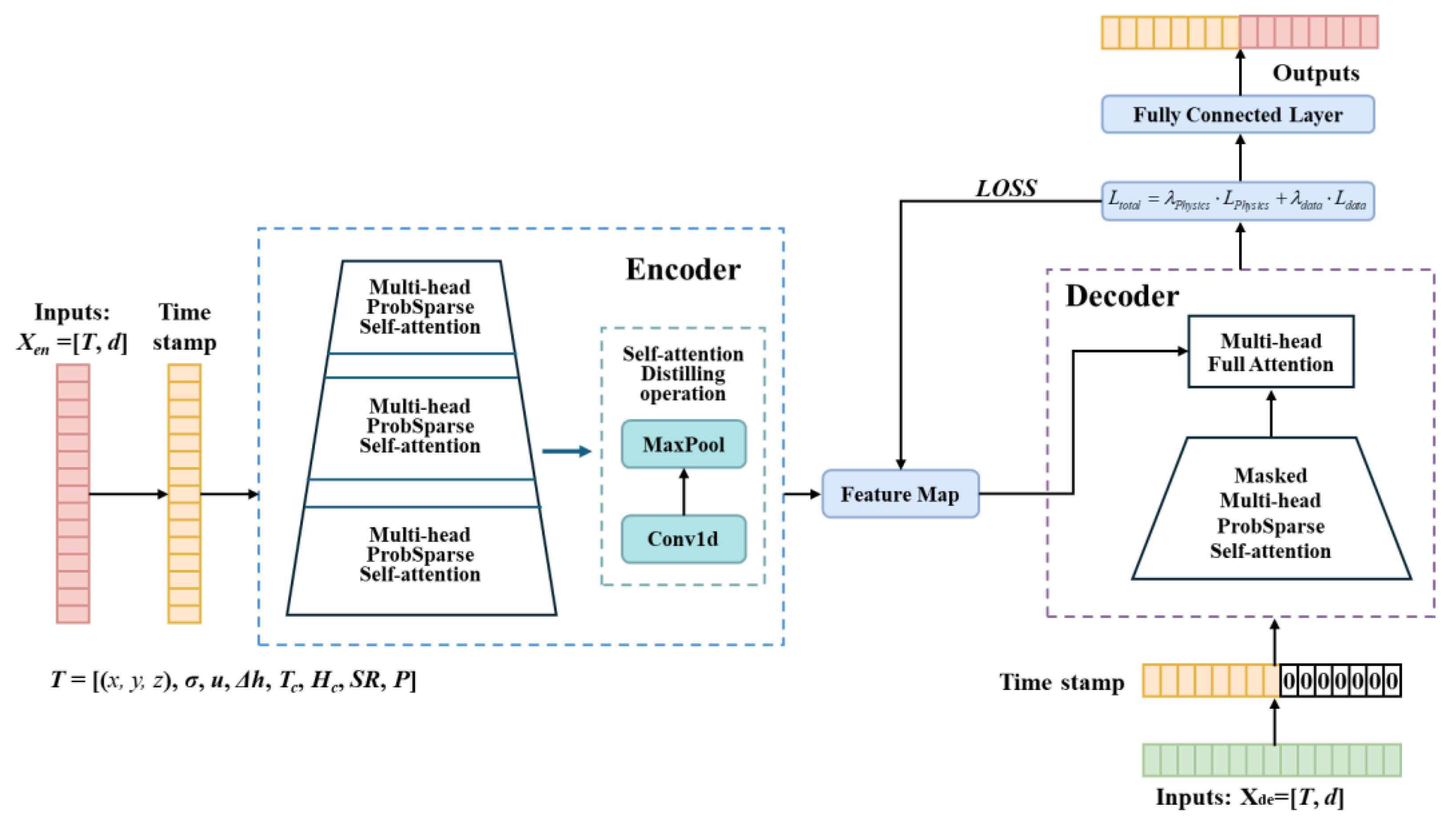
2.1.2. Informer Model for Long-Sequence Forecasting
The Informer model serves as the backbone of the PA-Informer framework, providing a highly efficient structure for long-sequence time-series forecasting. It addresses the computational inefficiencies of traditional Transformers while maintaining high accuracy for long input sequences through three core mechanisms: ProbSparse, self-attention distilling, and a generative-style decoder.
The ProbSparse mechanism reduces the computational complexity of traditional self-attention from O(L2) to O(L·lgL) by leveraging the sparsity assumption, which significantly improves memory efficiency while retaining the ability to capture long-range dependencies [24].
To enhance efficiency, Informer reduces sequence length after each attention layer by retaining dominant features through convolution and max-pooling. This operation halves the sequence length at each layer, minimizing memory usage to O((2-ɛ)·L·lgL) while preserving global dependencies. Additionally, stacking multiple encoder layers with reduced sequence lengths enables the model to extract multi-scale features and robust long-term patterns [25].
Instead of generating predictions step by step, the Informer decoder handles the entire target sequence in a single forward pass, avoiding cumulative error propagation. Using a start token and placeholders for the target sequence, it generates predictions directly, ensuring faster inference and high accuracy for long-sequence outputs. This makes it particularly suited for long-sequence time-series forecasting (LSTF) tasks [26].
2.1.3. Derivation of the Unified IRI Residual PDE
To ensure physics constraints in the IRI prediction task, the PA-Informer model incorporates a residual PDE that establishes the relationship between IRI, joint geometry, material properties, and environmental conditions. This PDE ensures that predictions adhere to the physical laws governing pavement roughness evolution.
IRI is an indicator used to measure the smoothness of a road surface. It is typically defined as the ratio of the cumulative vertical motion generated by a vehicle's suspension system during travel to the corresponding horizontal movement. Its formula is expressed as [27]:
Where zr’(x) represents the vehicle's vertical velocity and L is the road length. Taking into account the influence of joint geometry on vehicle vibration, the commonly used empirical formula for IRI can be expressed as [28]:
Where k1 and k2 are fixed values related to vehicle characteristics, ω represents the joint width, and represents the joint height difference. ω and can be associated with the internal stress field σ of the cement concrete slab through the mechanical equilibrium equation shown in Equation (4).
α and β represent the thermal expansion coefficient and hygroscopic expansion coefficient, respectively, while the strain tensor ɛ can be derived from the displacement field as:
The relationship between the stress field σ and the internal temperature field and humidity field of the cement concrete slab can be expressed by Equations (5) to (8):
By combining Equations (3) to (8), the residual expression of IRI can be derived and is simplified as Equation (9).
The specific meanings of the physical quantities are summarized in Table 1 as follows:
2.1.4. Integration of Informer with Physical Constraints
To achieve accurate predictions that are both informed by temporal patterns and consistent with physical laws, the PA-Informer model integrates the Informer architecture with the residual PDE for IRI. This integration is achieved by combining the temporal features extracted by the Informer encoder with the physically consistent features generated from the residual PDE. These features are fused through a dimension adjustment module to ensure compatibility and effective integration. The decoder then generates predictions based on this unified representation, capturing both long-term temporal dependencies and physical dynamics.
The total loss function for the PA-Informer model is defined as:
where Ldata is the data-driven loss capturing the temporal patterns in the input time series, and LPhysics is the residual PDE loss ensuring physics constraints. To dynamically balance the contributions of these two losses during training, a self-adaptive weighting strategy based on loss gradient scales is employed. This strategy ensures that the gradient contributions from each loss are balanced, preventing one loss from dominating the optimization process.
The weights λdata and λPhysics are dynamically adjusted during training based on the gradient magnitudes of the respective losses. Specifically, the gradient norms for each loss with respect to the model parameters are computed as:
where ||·|| denotes the gradient norm, and θ represents the model parameters [29,30,31]. The weights are then updated to inversely scale with the gradient magnitudes, ensuring that the loss with a higher gradient norm receives a smaller weight. The weight formulas are defined as:
This strategy balances the optimization contributions from the data-driven and physics-informed losses, allowing the model to adapt to varying task requirements or input window lengths during training. During training, the total loss Ltotal is minimized using gradient-based optimization. The dynamic weighting mechanism ensures that the contributions from Ldata and LPhysics are adjusted in real-time based on their respective gradient scales, promoting a balanced optimization process. This adaptive strategy is particularly effective when the scales or sensitivities of the two losses differ significantly or vary across training iterations.
3. Experiments
3.1. Data Collecting
The data utilized in this study were collected from long-term performance monitoring sites of cement concrete pavements located in various typical climatic regions across China. These monitoring sites are distributed across four representative environmental zones: arid desert region, humid and rainy region, lightly frozen region, and the Qinghai-Tibet alpine region. The primary focus of these sites is to monitor pavement performance under different climatic conditions over extended periods [30].
As shown in Table 2, four monitoring sites in Xinjiang, Guangxi, Beijing, and Tibet corresponding to one of the aforementioned climatic zones were established. The pavement structures and monitoring systems at each site were specifically designed to accommodate the unique geographic and climatic characteristics of their respective regions. Till now, the monitoring and data transmission systems at all sites have been operating stably. Between June 2022 and July 2025 (164 weeks in total), the data collection effort has yielded over 12.60 million records, providing a robust dataset for analyzing long-term pavement performance under diverse environmental conditions.
At each monitoring site, an integrated data acquisition system was installed to monitor the long-term performance of cement concrete pavements. The monitored parameters include:
- Meteorological Observations: Precipitation levels and solar radiation intensity are recorded by weather stations (Figure 2).
- Internal Temperature and Humidity Fields: Temperature and humidity distribution within the pavement structure is monitored using temperature and humidity fiber-optic sensors (Figure 3).
The layout of sensors embedded within the pavement structure is illustrated in Figure 4. All sensors collect data at a frequency of once every 5 seconds.
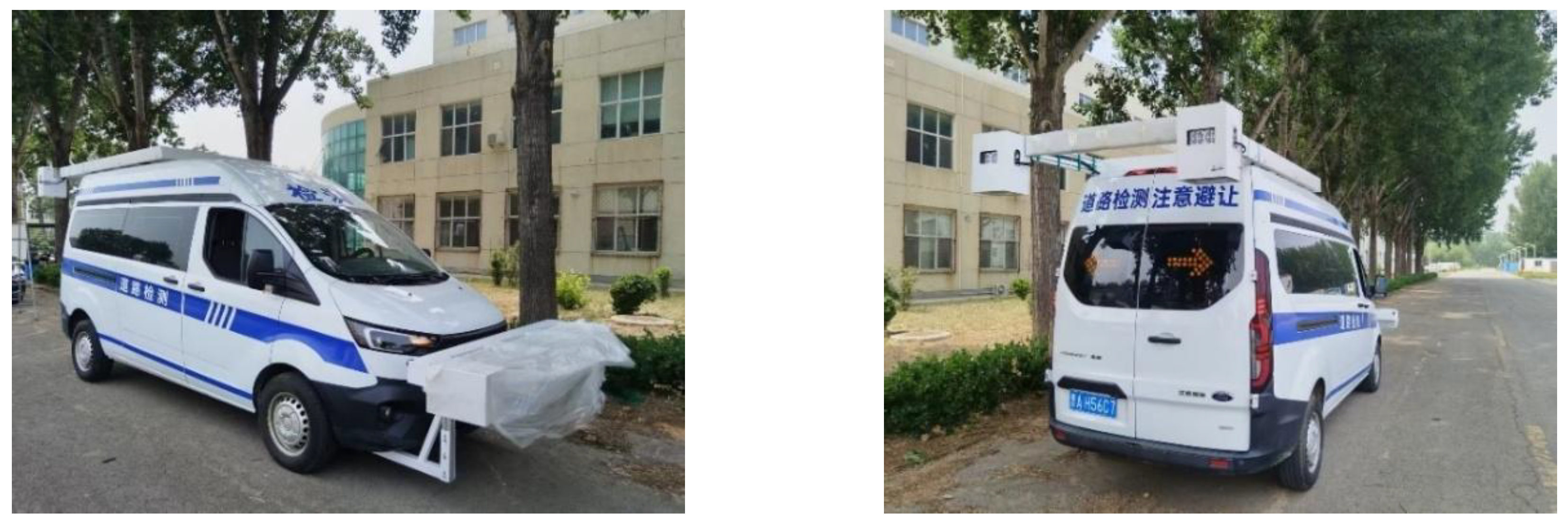
After the completion of pavement construction, weekly surface condition measurements are conducted at each monitoring site. Specifically, every Thursday, a road performance testing vehicle equipped with a LiDAR system (Figure 5) scans the pavement surface to obtain point cloud data. The point cloud data are then processed using Proval software, which extracts the pavement surface elevation data. From these, the pavement centerline IRI is calculated and used as one of the key feature indicators input into the prediction model.
Figure 6.
Overall layout diagram of the sensors.
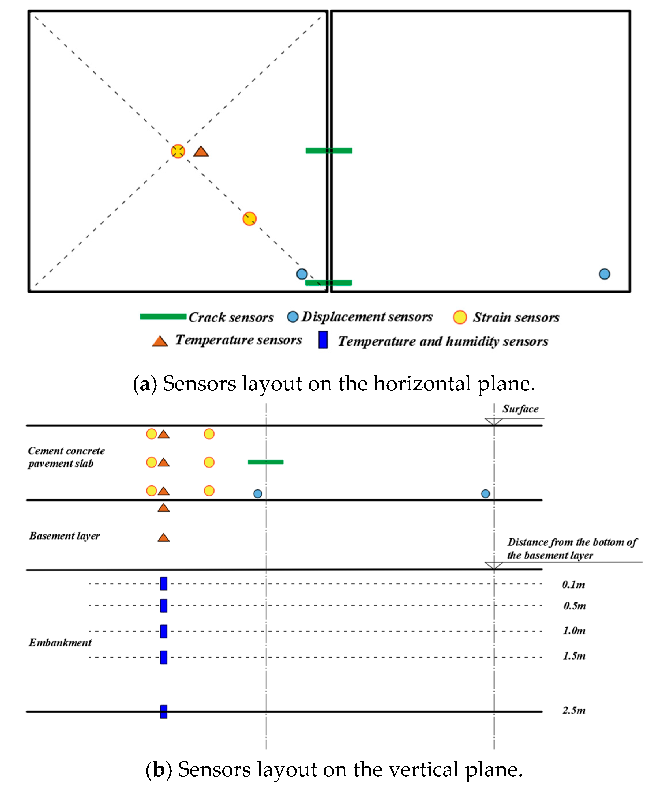
Figure 7.
Road performance testing vehicle.
3.2. Experiments Details
After the data was collected, all input data were preprocessed using zero-mean normalization, and input window lengths of 30, 60, 90, and 120 weeks were tested to explore the impact of sequence lengths on prediction performance. The data from Beijing, Guangxi, and Xinjiang spanning June 2022 to December 2024 were used as the training set, while data from January 2025 to August 2025 served as the validation set. Additionally, to evaluate the model’s generalization ability and robustness under extreme climatic conditions, data from Tibet during the same validation period were used as the test set.
Given that the input features are collected every 5 seconds, while the target variable, IRI, is measured on a weekly basis. It is necessary to align the temporal resolution of the target variable with that of the input features, for which a Gaussian interpolation method is employed to interpolate the IRI values, thereby matching the high temporal resolution of the input features. This approach generates a continuous and smooth IRI time series, ensuring consistency with the dimensions of other feature variables. Furthermore, it preserves the cumulative effects of certain variables without compromising their significance. By applying this feature-specific processing strategy, all input features were unified to a weekly temporal resolution that matched the IRI measurements. The processed weekly features were then concatenated into input windows of varying lengths (30, 60, 90, and 120 weeks) to explore the impact of temporal sequence lengths on model prediction performance.
To prepare the data for the encoder, the processed features are structured into an input matrix with a shape of (T,d), where T represents the length of the input window, and d represents the number of features after preprocessing. Additionally, time stamps are incorporated into the input matrix to encode temporal information explicitly. The input matrix, augmented with temporal information, is then fed into the encoder. The encoder would extract high-level temporal patterns and dependencies from the input data, producing a context vector that served as the foundation for the subsequent prediction tasks.
To validate the predictive accuracy and generalizability of the model, four evaluation metrics were selected: Mean Squared Error (MSE), Coefficient of Determination (R2), and the Sensitivity Coefficient (Sp). The mathematical formulations of these metrics are presented in Table 3. By leveraging these diverse evaluation criteria, the study ensures a robust and thorough evaluation of the model’s effectiveness under varying conditions.
Mean Squared Error (MSE) quantifies the average squared difference between the predicted and true values, providing a direct measurement of the model’s accuracy, where lower MSE values indicate better performance as they reflect smaller deviations from the ground truth [35]. Similarly, the Coefficient of Determination (R2) measures the proportion of variance in the target variable explained by the model’s predictions, evaluating the model’s goodness-of-fit, with values closer to 1 demonstrating higher explanatory power [36]. Finally, the Sensitivity Coefficient (Sp) quantifies the influence of input parameters (p) on the predicted IRI values by adjusting the perturbation value (Δp) of input variables and observing changes in IRI, where larger (Sp) values indicate a more significant driving effect of the parameter on IRI variations [37]. Together, these metrics provide a comprehensive evaluation of the model’s accuracy, explanatory power, temporal alignment, and sensitivity to input parameters.
4. Results and Discussion
4.1. Hyperparameters Tuning Process
The initial hyperparameters of the model are determined based on prior knowledge of the Informer architecture and the characteristics of the dataset. Studies have shown that Transformer models effectively could capture long-term dependencies in time series data through multi-head self-attention mechanisms and feed-forward neural networks [4,5]. By introducing the ProbSparse attention mechanism, Informer reduces the computational complexity of self-attention for long input sequences. Thus, the encoder and decoder are configured with 3 and 2 layers, respectively, to ensure the capacity for modeling long-term dependencies while maintaining computational efficiency.
The token embedding dimension was set to 5 to provide a compact representation of input features, according to the recommended lightweight embedding dimensions for time series tasks [4]. The hidden layer dimension of the feed-forward neural network (FFNN) was set to 20, which is four times the token embedding dimension, to balance model complexity and generalization performance. The initial learning rate was set to 0.0001 with a decay factor of 0.5 to stabilize the training process as the model converges. The number of training epochs was set to 100 to ensure sufficient iterations for learning complex temporal patterns, while the batch size was configured to 32 to balance computational efficiency and gradient stability. The weights for the physics-constrained loss (LPhysics) and data-driven loss (LData) were initialized to 0.1 and 0.9, respectively.
To optimize the model performance, a systematic hyperparameter tuning process was carried out, combining grid search, residual analysis and dynamic loss weight adjustment methods. The optimization process mainly adjusted key parameters such as the learning rate, batch size, training rounds, and loss weight balance. To ensure that the original long sequences of the Informer model pay particular attention to the relationship between residual weights and the length of the time series. The learning rate (k) is fine-tuned within the range of [0.0001,0.01] to determine the optimal convergence rate [5]. A larger learning rate will lead to unstable training dynamics, while a smaller learning rate could result in excessively slow convergence. Consequently, a learning rate of 0.001 and a decay factor of 0.8 are selected as the optimal values to balance convergence speed and training stability. The batch size is adjusted between 16 and 64 to evaluate its impact on memory usage and training efficiency [38]. A batch size of 32 achieved the best balance between gradient stability and computational efficiency. Adjustments to the model architecture involve varying the number of encoder and decoder layers to balance model capacity and computational feasibility. Experimental results show that the encoder with over 4 layers provides limited improvement in prediction accuracy, while reducing them to 2 resulted in a significant drop in performance. Ultimately, a configuration of 3 encoder layers and 2 decoder layers is retained.
As described in Section 2.2.4, a dynamic weight adjustment mechanism to adapt the weights of the physics-constrained loss (λPhysics) and the data-driven loss (λdata) based on the length of the time series is used in the PA-Informer model. Through model training and fine-tuning, it is determined that for time series lengths of 30, 60, 90, and 120, the corresponding residual weights are set as (λPhysics, λdata) = (0.46, 0.54), (0.39, 0.61), (0.33, 0.67), and (0.18, 0.82), respectively. The balance effectively promotes both physics constraints and prediction accuracy, which significantly improves the model’s generalization ability across different time series lengths.
After determining other hyperparameters, the number of epochs was adjusted by analyzing the convergence process of the residual curves. Residual analysis was conducted to study the convergence speed and process of the PA-Informer and Informer models on datasets from Beijing, Guangxi, Xinjiang, and Tibet. Compared to the Informer model, the PA-Informer model demonstrated significantly faster convergence speeds and a more stable residual reduction process across all regional datasets. When the input window is 30, the PA-Informer model had the slowest convergence speed compared to input windows of 60, 90, and 120. However, even in this case, the PA-Informer model’s residuals can still converge to below 0.05 within 20 training epochs, whereas the Informer model exhibits a much slower convergence speed and pronounced oscillations, particularly on the Xinjiang and Tibet datasets. Such results indicate that the PA-Informer model’s faster and smoother convergence process enables it to better adapt to the diverse dynamic characteristics of regional datasets, achieving higher prediction accuracy and robustness. For the PA-Informer model, validation loss stabilizes after approximately 15 training epochs, suggesting that the initially set 100 training epochs may not be optimal. To improve training efficiency and prevent overfitting, an early stopping mechanism is introduced, terminating training when the validation loss shows no improvement for 20 epochs [39]. In conclusion, the final hyperparameter settings are shown in Table 4. The Informer baseline model used for comparison adopts the exact same architecture and hyperparameter settings as the PA-Informer model.
4.2. Prediction Accuracy Evaluation
To quantitatively analyze the prediction accuracy, the MSE and R2 on both training and test set are calculated and shown in Figure 8 and Figure 9.
In Figure 8 and Figure 9a, a horizontal comparison of the MSE and R2 values across different models shows that, except for the MR model, the prediction accuracy of all other models improves as the time series length increases. The proposed PA-Informer model achieves a maximum MSE of 0.0165 (input window length of 30 weeks) and a minimum MSE of 0.0152 (input window length of 120 weeks) on the training and testing datasets, with an MSE variation of less than 8.55%. While ensuring the smallest MSE (0.0152) and the highest R² (0.985) on the testing set, the PA-Informer model also exhibits the smallest fluctuation range, which suggests that within the input window length range from 30 to 120 weeks, reducing the input window length has minimal impact on the performance of the PA-Informer model. Even for shorter time series, the model maintains reliable prediction accuracy. Figure 9b illustrates the models’ R2 on the Tibet testing dataset, where the high consistency between actual data and predictions demonstrates the strong ability to capture underlying patterns. This further validates the reliability and generalizability of the PA-Informer model in complex environments.
The instability observed in other models is primarily due to significant differences in regional meteorological conditions, such as precipitation, sunlight, temperature, and humidity, which have vastly different effects on cement concrete. Without the constraints of physical consistency, the cumulative effects of these meteorological factors on IRI can greatly influence the IRI prediction ability of the models. In Xinjiang, the dry climate and intense sunlight primarily impact IRI through temperature stress, whereas in Guangxi, IRI variations are more influenced by precipitation and humidity. Under such complex and variable climatic conditions, traditional time series models often struggle to maintain predictive accuracy for shorter time series due to insufficient dynamic information. In contrast, the proposed PA-Informer model incorporates a Physical-Aware approach by integrating partial differential equations (PDEs) as residual equations into the model. By leveraging physics constraints, this approach addresses the original Informer model’s performance limitations with a shorter input window. Generally, the PA-Informer model demonstrates superior predictive accuracy and stability across various input window lengths and diverse climatic conditions.
4.3. Sensitivity Analysis
Based on the results in Section 4.2 regarding model prediction accuracy, this section further analyzes the reasons behind the performance differences among models by incorporating sensitivity analysis. For this analysis, only the Informer and LSTM-MA models, whose performance is closest to the PA-Informer model, are selected for comparison. Both models use an input window length of 120 weeks, which yielded their best prediction performance.
Figure 10.
Sensitivity analysis for different feature indicators (u, σ, SR, and P).
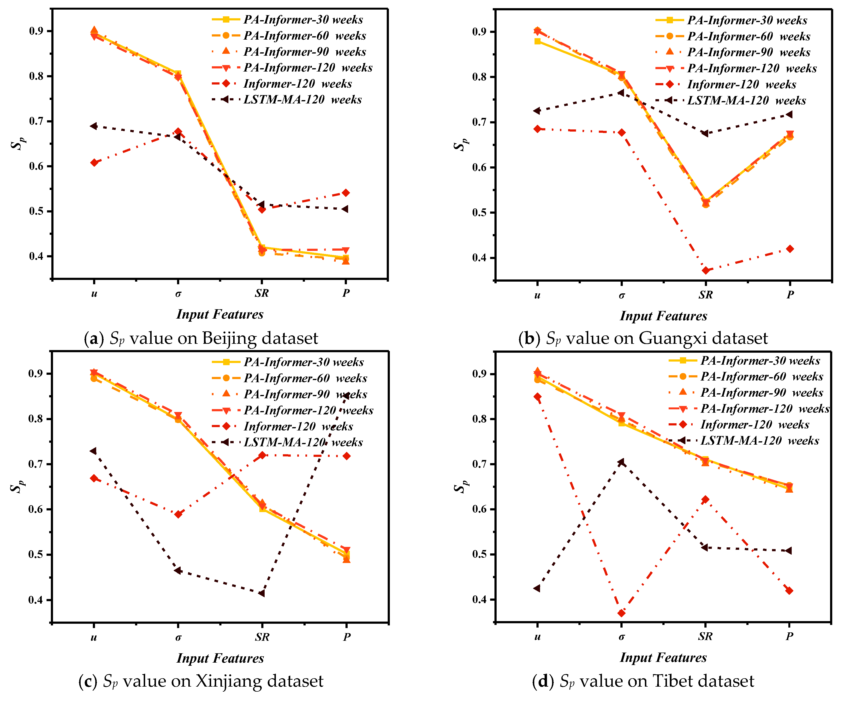
Figure 11.
Residual curve graphs of PA-Informer and Informer models with different time series lengths (BJ: Beijing; GX: Guangxi; XJ: Xinjiang; TB: Tibet).
Figure 11.
Residual curve graphs of PA-Informer and Informer models with different time series lengths (BJ: Beijing; GX: Guangxi; XJ: Xinjiang; TB: Tibet).
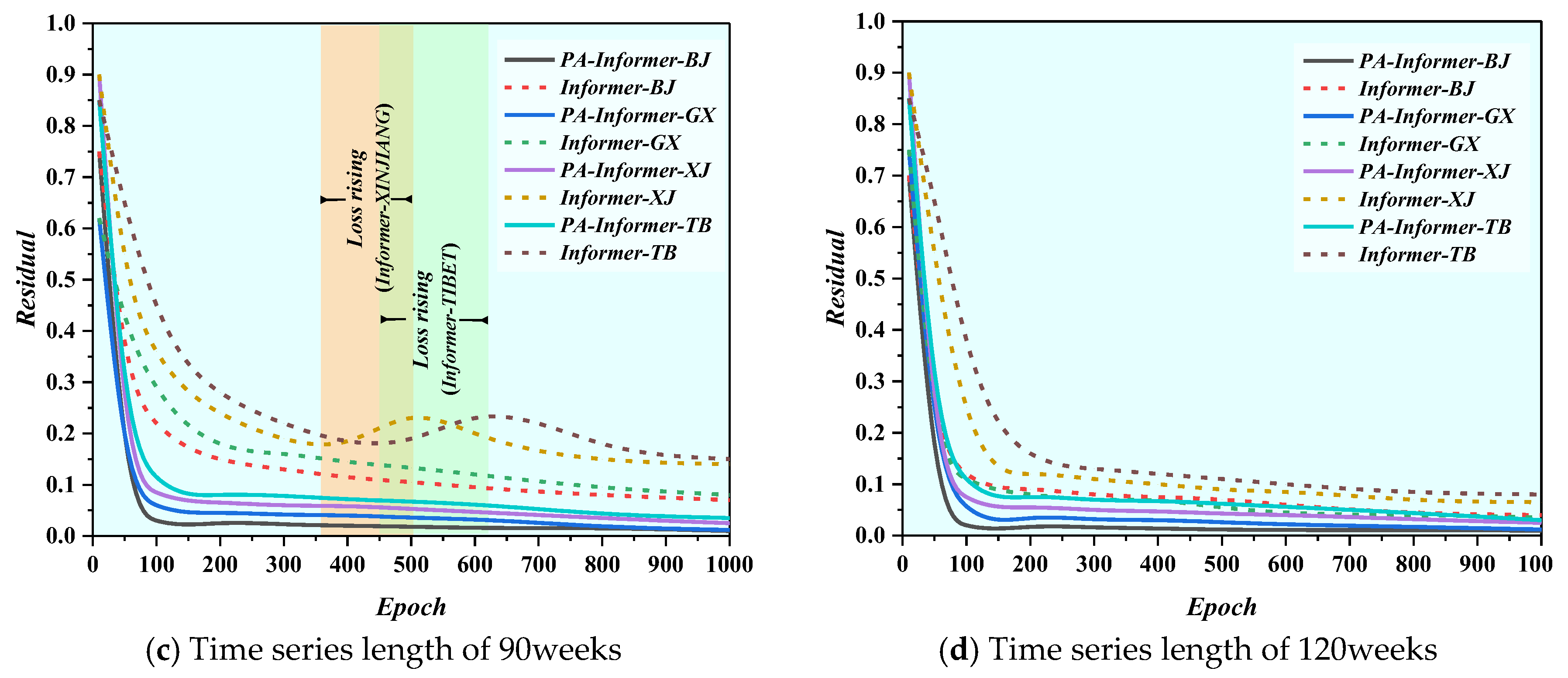
Regardless of input window length, the PA-Informer model demonstrates Sp value variations of less than 5% for different input feature indicators across all datasets, which indicates that the PA-Informer model can accurately capture the influence of various indicators on IRI changes with minimal impact from input window length. This performance improvement can be attributed to the enhanced Physical-Aware mechanism, which enables the model to better capture the relationships between features and IRI even under shorter input window conditions. To some extent, this suggests that the sensitivity captured by the PA-Informer model is effective and can serve as a baseline for comparisons with other models.
The Sp values of the same feature indicator vary across regions due to differences in climatic conditions, which significantly affect the impact of physical features on IRI changes. On any dataset, the PA-Informer model consistently identifies joint displacement as the most sensitive feature (Sp around 0.9), followed by internal stress (Sp around 0.8), both of which keep relatively stable. But SR and P have lower sensitivity varying as the dataset changes. In arid desert regions, Xinjiang, due to frequent thermal expansion and contraction cycles, the large diurnal temperature variations will highly influence joint displacement (Sp ≈ 0.91). intense solar radiation (Sp ≈ 0.62) amplifies the temperature gradient and increases internal stress (Sp ≈ 0.85). Conversely, in humid and rainy region, Guangxi, except for joint displacement and internal stress, P becomes the dominant factor (Sp ≈ 0.67) higher than the sensitivity of SR (Sp ≈ 0.52). As excessive water infiltration into concrete pavements exacerbates joint spalling and subgrade erosion, which accelerates the growth of IRI. In high-altitude cold regions, Tibet, the frequent freeze-thaw cycles drive significant joint displacement (Sp ≈ 0.95), while solar radiation (Sp ≈ 0.65) and precipitation (Sp ≈ 0.71) jointly contribute to rapid IRI growth due to extreme environmental variability. Finally, in lightly frozen regions (e.g., Beijing), where climatic conditions are relatively moderate, joint displacement (Sp ≈ 0.82) and internal stress (Sp ≈ 0.78) remain the primary influencing factors, with lower sensitivity to SR and P (both ≈ 0.41).
Furthermore, interaction effects between features amplify their impact under specific climatic conditions. In high-altitude regions, freeze-thaw cycles combined with intense solar radiation significantly accelerate joint displacement and stress accumulation, leading to faster IRI growth [40]. Similarly, in humid regions, prolonged precipitation coupled with temperature fluctuations exacerbates subgrade settlement, highlighting the compound effect of multiple features on pavement deterioration.
In comparison, the Informer and LSTM-MA models exhibit no clear patterns in the sensitivity changes of various features. On the Beijing dataset, these models can still identify higher sensitivity for joint displacement and internal stress compared to SR and P. Similarly, the Informer model on the Guangxi dataset can identify changes in the four key features similar to the PA-Informer model. However, as climatic conditions become more complex, these models struggle to identify the dependency relationships between feature parameters and IRI trend changes.
Overall, the PA-Informer model demonstrates not only the ability to maintain stable sensitivity to input feature indicators regardless of input window length but also the flexibility to adapt to regional variations in feature sensitivity under different climatic conditions. This highlights the model's superior robustness and adaptability compared to other models.
5. Conclusions
This study introduces the Physics Aware-Informer (PA-Informer) model, a hybrid framework that combines the Informer structure with physics constraints to achieve accurate and robust IRI predictions for pavement performance monitoring. By embedding residual PDEs into the model, the PA-Informer ensures that predictions align with the governing physical laws of pavement roughness evolution. The dynamic weighting strategy enables the model to adapt to different input window lengths and environmental conditions, making it suitable for diverse applications.
Experimental results based on four representative climatic zones in China (arid desert, humid and rainy, lightly frozen, and high-altitude cold regions) validate the effectiveness of the model. The PA-Informer achieves an MSE of 0.0165 and R² of 0.962 for a 30-week input sequence and an MSE of 0.0152 and R² of 0.985 for a 120-week input sequence. Sensitivity analysis highlights that joint displacement (Sp ≈ 0.89) and internal stress (Sp ≈ 0.81) are the most significant factors influencing IRI. And compared with the best prediction results of other models, the PA-Informer model can keep the sensitivity of each feature index stable during the process of the length change of the input window. While other models can maintain a relatively good level of prediction accuracy, they cannot capture the dependent features corresponding to IRI under more complex meteorological conditions. Generally, the model exhibits stable performance across different climatic conditions, demonstrating its robustness and adaptability.
Despite its advantages, the PA-Informer model has certain limitations. First, the computational cost of incorporating PDE constraints increases with the complexity of the equations and the number of influencing factors. Second, the model relies on high-quality and diverse input data, potentially limiting its performance in scenarios with noisy or incomplete datasets. Third, the interpretability of the interaction between the Informer and PDE components requires further enhancement for broader usability. Finally, the current dataset is limited to regions in China, which may restrict the generalizability of the model.
Future research shall focus on: (1) Optimizing computational efficiency by exploring lightweight PDE approximation methods and model pruning techniques. (2) Enhancing data preprocessing procedure to handle incomplete datasets more effectively. (3) Expanding dataset diversity by incorporating international datasets, such as the Long-Term Pavement Performance (LTPP) program, to further validate and enhance the model’s generalizability. (4) Incorporating additional factors such as maintenance history to develop a more comprehensive pavement performance prediction framework.
By addressing these challenges, the PA-Informer framework can be further refined to become a more efficient, interpretable, and globally applicable tool for time-series forecasting in transportation infrastructure.
References
- T. Zhang, A. Smith, H. Zhai, Y. Lu. LSTM+MA: A Time-Series Model for Predicting Pavement IRI. Infrastructures 2025, 10, 10. [Google Scholar] [CrossRef]
- Dalla Rosa, F. , Liu L., & Gharaibeh, N. G. IRI prediction model for use in network-level pavement management systems. Journal of Transportation Engineering, Part B: Pavements, 2017, 143, 04017001. [Google Scholar] [CrossRef]
- Hochreiter, S. & Schmidhuber, J. Long short-term memory. Neural Computation, 1997, 9, 1735–1780. [Google Scholar]
- Zhou, H. , Zhang S., Peng J., et al. Informer: Beyond efficient transformer for long sequence time-series forecasting. Proceedings of the AAAI Conference on Artificial Intelligence, 2021, 35, 106–115. [Google Scholar] [CrossRef]
- Vaswani A., Shazeer N., Parmar N., et al. Attention is all you need. Advances in Neural Information Processing Systems, 2017, 30.
- Marcelino, P. , de Lurdes Antunes M., & Gomes M. C. Machine learning approach for pavement performance prediction. International Journal of Pavement Engineering, 2021, 22, 341–354. [Google Scholar]
- Qin Y., Song D., Chen H., et al. A dual-stage attention-based recurrent neural network for time series prediction. Proceedings of the 26th International Joint Conference on Artificial Intelligence, 2017, 2627-2633.
- Deng, F. , Tang X., & Wu T. Particle swarm optimization-augmented feedforward networks for pavement rutting prediction. Journal of Computing in Civil Engineering, 2015, 29, 04014097. [Google Scholar]
- Wang, K. , Huang Y., & Zhang Z. Hybrid gray relation analysis and support vector regression for pavement performance prediction. International Journal of Pavement Research and Technology, 2018, 11, 287–294. [Google Scholar]
- Gong, W. , Chen H., & Zhang J. Random forest regression for flexible pavement IRI modeling. Transportation Research Record: Journal of the Transportation Research Board, 2019, 2673, 299–309. [Google Scholar]
- Damirchilo, B. , Yazdani R., & Khavarian M. XGBoost-based pavement performance prediction and handling missing values. International Journal of Pavement Engineering, 2020, 21, 456–466. [Google Scholar]
- Song, Y. , Wang L., & Yin J. ThunderGBM-based ensemble learning for asphalt pavement IRI prediction. Construction and Building Materials, 2021, 313, 125421. [Google Scholar]
- Zhou, X. , Li, J., & Fang, S. RNN-based models for asphalt pavement performance prediction using LTPP data. International Journal of Pavement Research and Technology, 2018, 11, 559–567. [Google Scholar]
- Han, Z. , Liu, F., & Zhang, X. Modified RNN for falling weight deflectometer back-calculation. Journal of Computing in Civil Engineering, 2020, 34, 04020023. [Google Scholar]
- Raissi, M. , Perdikaris, P., & Karniadakis, G. E. Physics-informed neural networks: A deep learning framework for solving forward and inverse problems involving PDEs. Journal of Computational Physics, 2019, 378, 686–707. [Google Scholar]
- Karniadakis G., E. , Kevrekidis I. G., Lu L., et al. Physics-informed machine learning. Nature Reviews Physics, 2021, 3, 422–440. [Google Scholar] [CrossRef]
- Sun, L. , Wang Z., & Zhang H. Physics-informed deep learning for time-series forecasting in engineering applications. Mechanical Systems and Signal Processing, 2021, 152, 107377. [Google Scholar]
- Tartakovsky A., M. , Marrero C. O., Perdikaris P., et al. Physics-informed deep neural networks for learning parameters and constitutive relationships in subsurface flow problems. Water Resources Research, 2020, 56, e2019WR026731. [Google Scholar] [CrossRef]
- Lu, L. , Meng, X., Mao, Z., & Karniadakis, G. E. DeepXDE: A deep learning library for solving differential equations. SIAM Review, 2021, 63, 208–228. [Google Scholar]
- H. Dai, Z. Liu, J. Dai, Y. Liu, An adaptive spatio-temporal attention mechanism for traffic prediction. IEEE Internet of Things Journal, 2021, 8, 11915–11924. [Google Scholar]
- Z. Xu, C. Feng, L. Zhang, Physics-enhanced neural networks for multiscale spatiotemporal traffic prediction. Transportation Research Part C: Emerging Technologies, 2022, 137, 103597. [Google Scholar]
- Sun, L. , Wang Z., & Zhang H. Physics-informed deep learning for time-series forecasting in engineering applications. Mechanical Systems and Signal Processing, 2021, 152, 107377. [Google Scholar]
- Raissi, M. , Perdikaris P., & Karniadakis G. E. Physics-informed neural networks: A deep learning framework for solving forward and inverse problems involving PDEs. Journal of Computational Physics, 2019, 378, 686–707. [Google Scholar]
- Child, R. , Gray S., Radford A., & Sutskever I. Generating long sequences with sparse transformers. arXiv preprint, arXiv:1904.10509.
- Beltagy, I. , Peters M. E., & Cohan A. Longformer: The long-document transformer. arXiv preprint, arXiv:2004.05150.
- Vaswani A., Shazeer N., Parmar N., Uszkoreit J., Jones L., Gomez A. N., Kaiser Ł., & Polosukhin I. Transformer-XL: Attentive language models beyond a fixed-length context. Proceedings of the 57th Annual Meeting of the Association for Computational Linguistics, 2019, 2978–2988.
- Sayers M. W., Gillespie T. D., & Paterson W. D. O. Guidelines for conducting and calibrating road roughness measurements. World Bank Technical Paper, 1986, 46.
- Sayers M. W., & Karamihas S. M. The Little Book of Profiling: Basic Information about Measuring and Interpreting Road Profiles. University of Michigan, Transportation Research Institute, 1998.
- Chen Z., Badrinarayanan V., Lee C. Y., & Rabinovich A. GradNorm: Gradient normalization for adaptive loss balancing in deep multitask networks. Proceedings of the 35th International Conference on Machine Learning (ICML), 2018, 807-815.
- Sener, O. , & Koltun V. Multi-task learning as multi-objective optimization. Advances in Neural Information Processing Systems (NeurIPS), 2019, 32, 527–538. [Google Scholar]
- Wang S., Teng Y., Perdikaris P., & Karniadakis G. E. Learning physics-informed neural networks without stacked back-propagation. arXiv preprint, 2021.
- Chatterjee, S. , & Singh B. Durability of concrete in an arid environment: Challenges and remedies. Construction and Building Materials, 2019, 223, 72–80. [Google Scholar]
- Mehta P. K., & Monteiro P. J. M. Concrete: Microstructure, Properties, and Materials. McGraw-Hill Education, 2014.
- Vaitkus, A. , Čygas D., Laurinavičius A., & Perveneckas Z. Analysis and evaluation of asphalt pavement structure damages caused by frost. The Baltic Journal of Road and Bridge Engineering, 2009, 4, 196–202. [Google Scholar]
- Willmott C., J. , & Matsuura K. Advantages of the mean absolute error (MAE) over the root mean square error (RMSE) in assessing average model performance. Climate Research, 2005, 30, 79–82. [Google Scholar]
- Steel R. G. D., Torrie J. H., & Dickey D. A. Principles and Procedures of Statistics: A Biometrical Approach. McGraw-Hill Education, 1997.
- Saltelli A., Ratto M., Andres T., Campolongo F., Cariboni J., Gatelli D., Saisana M., & Tarantola S. Global Sensitivity Analysis: The Primer. John Wiley & Sons, 2008.
- Goodfellow, I., Bengio, Y., & Courville, A. Deep Learning. MIT Press, 2016.
- Prechelt, L. Early stopping — But when? In Neural Networks: Tricks of the Trade (pp. 55–69). Springer, 1998.
- Li N., Zhang J., & Peng Z. Influence of environmental factors on the deterioration of concrete pavements in cold regions. Cold Regions Science and Technology, 2012, 83-84, 59-66.
Figure 2.
Weather station.
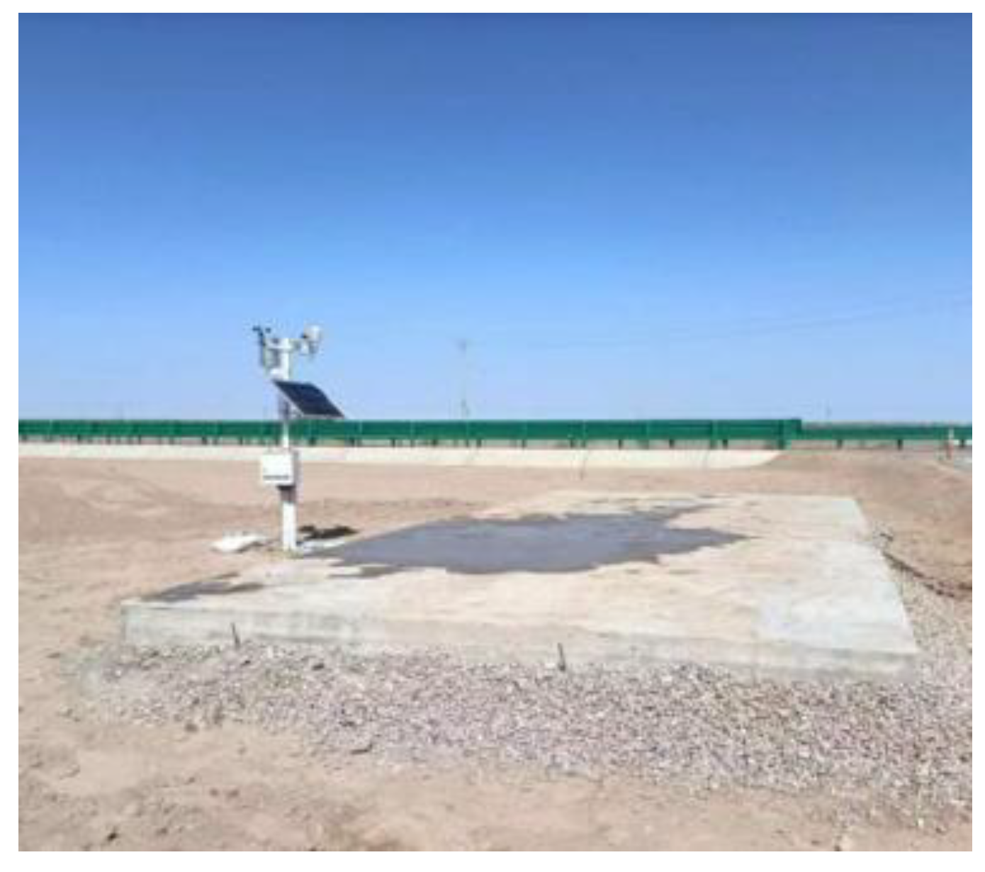
Figure 3.
Temperature and humidity sensors.
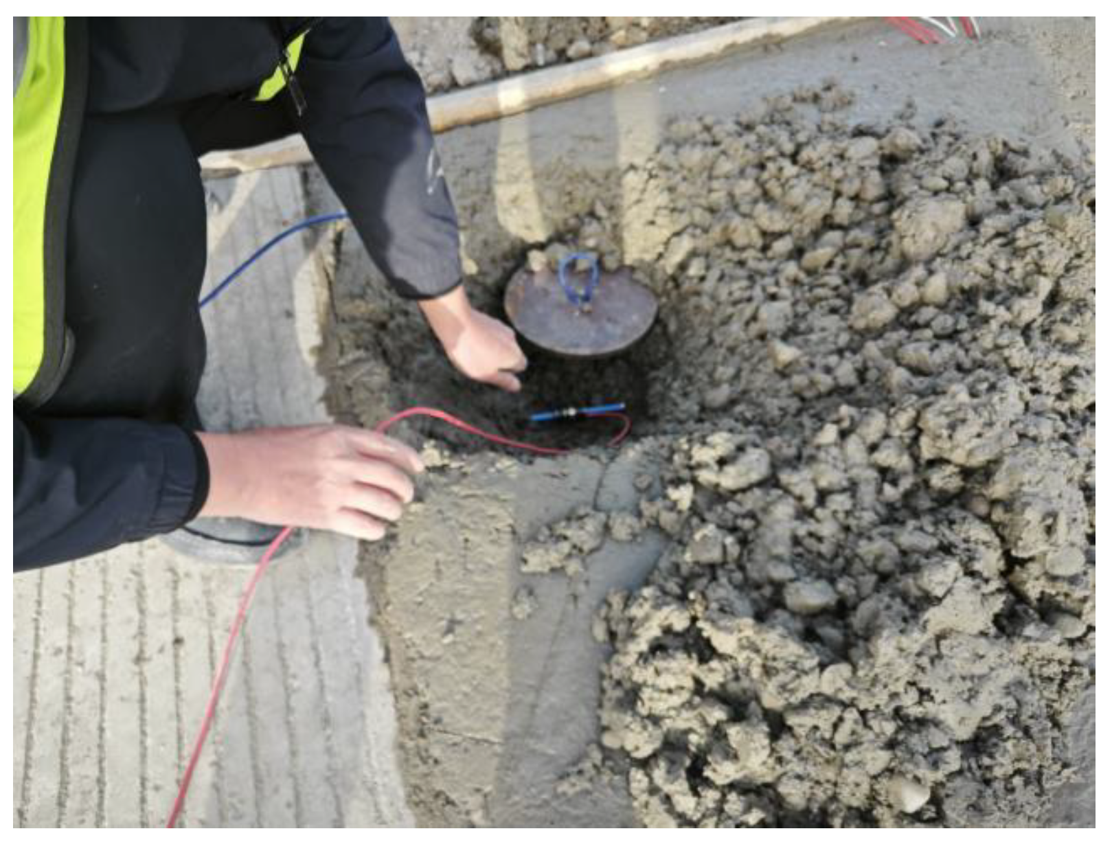
Figure 4.
Strain and stress sensors.
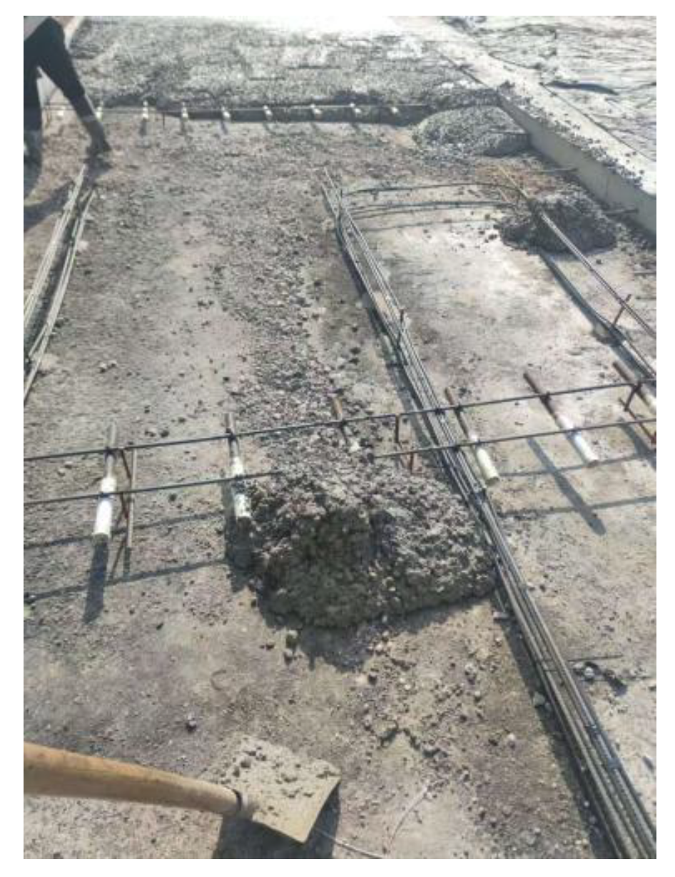
Figure 5.
Joint Fiber Optic Displacement Sensor.
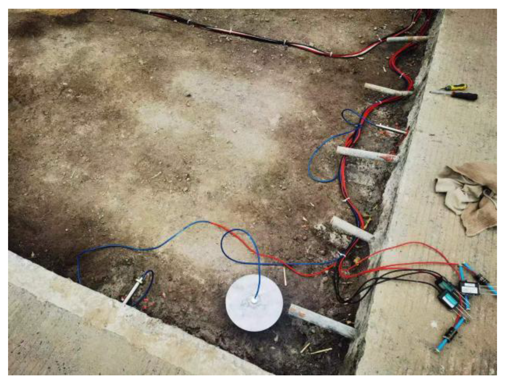
Figure 8.
The MSE curves of the selected models.
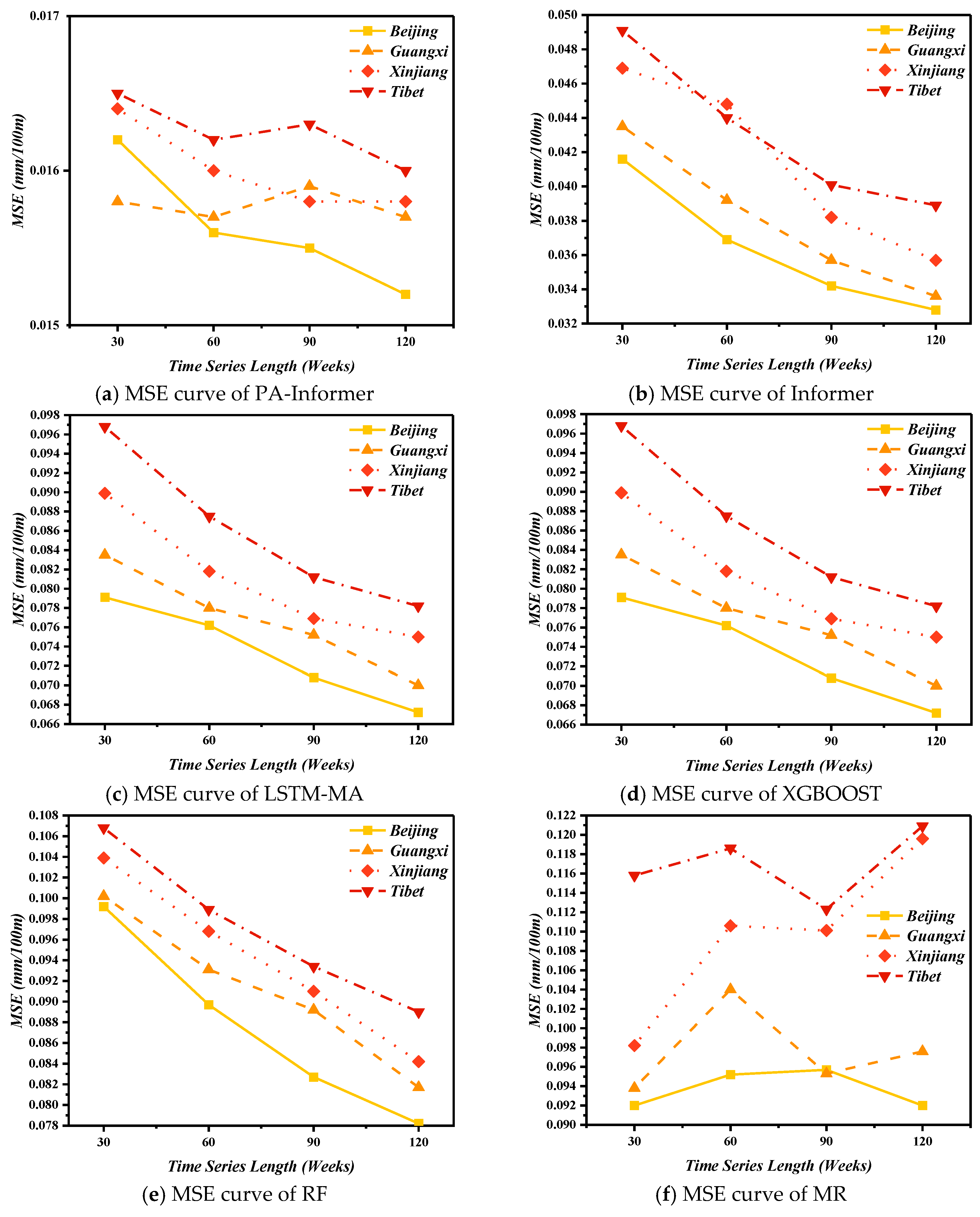
Figure 9.
Performance comparison of different models with a input window length of 120weeks.
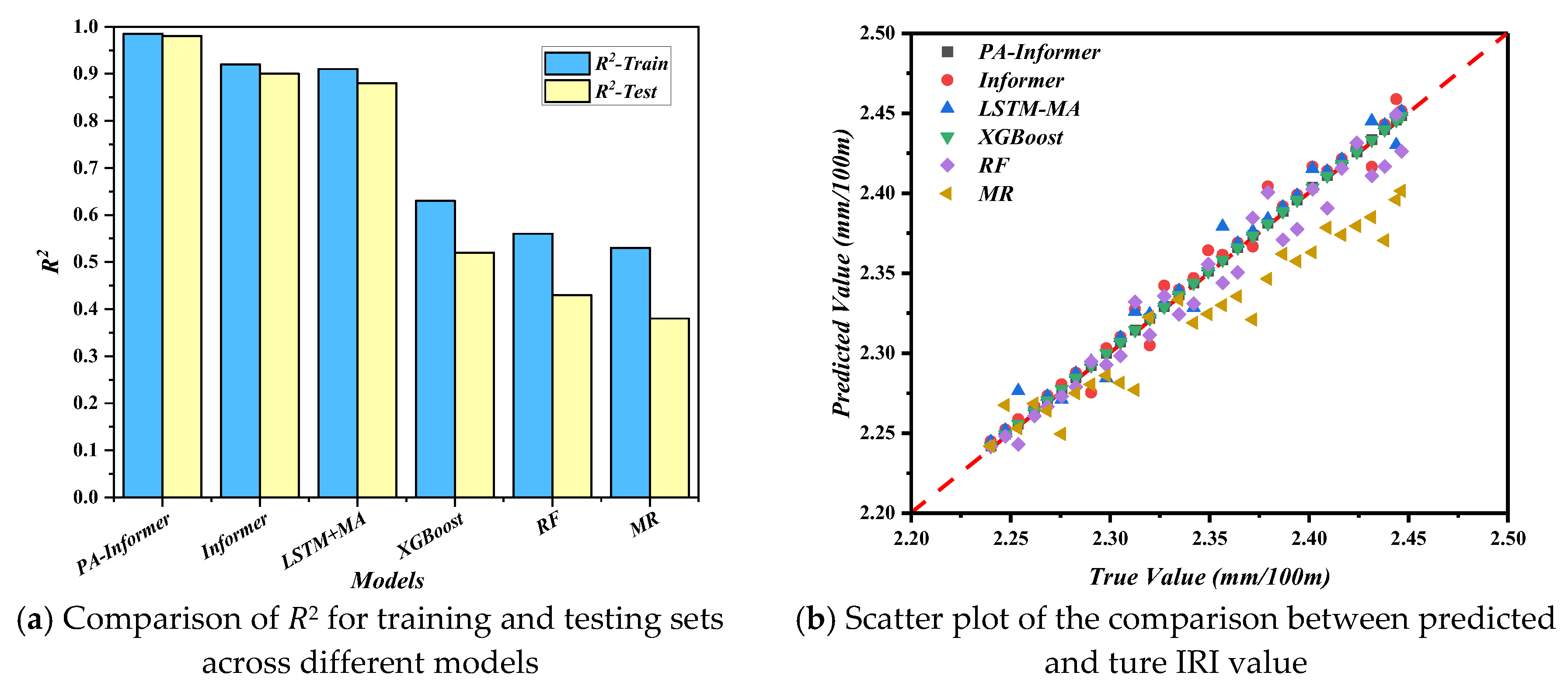

Table 1.
The parameters of environment and materials.
| Symbol | Physical Meaning |
| x, y, z | Coordinate |
| t | Time stamp |
| σ | Internal stress |
| u | Horizonal displacement at joints |
| Height difference at the joint | |
| L | Length of the road (In this study, L is fixed at 100 m) |
| Fourth-order elastic stiffness tensor, defined by E and v | |
| I | Cubic tensor |
| T | Atmospheric temperature |
| Tc | Internal temperature of cement concrete |
| Hc | Internal humidity of cement concrete |
| α | Thermal Expansion Coefficient |
| β | Hygroscopic Expansion Coefficient |
| SR | Solar Radiation |
| P | Precipitation |
| κT | Thermal conductivity |
| DH | Moisture diffusion coefficient |
Table 2.
Characteristics of typical environmental conditions of observation points.
| Dataset Types | Typical Environments | Characteristics of Natural Conditions of the Pavements | Provinces |
| Training set | Arid desert | In the arid desert region, cement concrete pavements face challenges from thermal expansion and contraction due to extreme temperature fluctuations, leading to frequent cracking and joint damage. Sand erosion can abrade the pavement surface, while dust accumulation may reduce skid resistance [32]. | Xinjiang |
| Hot and humid | In humid and rainy regions, excessive moisture infiltrates concrete pavements, causing joint spalling, surface scaling, and subgrade erosion. Persistent water exposure can also lead to damage at joints and cracks, accelerating structural deterioration [33]. | Guangxi | |
| Lightly frozen | Concrete pavements in light ice regions are affected by freeze-thaw cycles, which cause frost heave, cracking, and surface scaling. De-icing chemicals exacerbate surface deterioration and may lead to joint damage, weakening the cement concrete pavement over time [34]. | Beijing | |
| Test set | High-Altitude Cold Region | In Qinghai-Tibet Plateau, the extreme cold and presence of permafrost cause significant frost heave and thaw settlement, leading to uneven surfaces and cracking in concrete pavements. The harsh environment accelerates damage to joints and surface layers, reducing durability [32]. | Tibet |
Table 3.
The corresponding formulas of the indicators.
| Indicators | Formulas |
| MSE | |
| R2 | |
| Sp |
Table 4.
Value of hyperparameters.
| Hyperparameters | Initial Value | Final Value |
| Encoder layers | 3 | 3 |
| Decoder layers | 2 | 2 |
| Token embedding dimension | 5 | 5 |
| Dimension of the hidden layer of Feed-Forward Neutral Network | 20 | 20 |
| Learning rate | 0.0001 | 0.001 |
| Learning rate decay | 0.5 | 0.8 |
| Epoch | 100 | 20 |
| Batch size | 32 | 32 |
| λPhysics & λdata | 0.1 & 0.9 | 0.46 & 0.54 |
| 0. 39 & 0.61 | ||
| 0.33 & 0.67 | ||
| 0.21 & 0.79 |
Disclaimer/Publisher’s Note: The statements, opinions and data contained in all publications are solely those of the individual author(s) and contributor(s) and not of MDPI and/or the editor(s). MDPI and/or the editor(s) disclaim responsibility for any injury to people or property resulting from any ideas, methods, instructions or products referred to in the content. |
© 2025 by the authors. Licensee MDPI, Basel, Switzerland. This article is an open access article distributed under the terms and conditions of the Creative Commons Attribution (CC BY) license (http://creativecommons.org/licenses/by/4.0/).
Copyright: This open access article is published under a Creative Commons CC BY 4.0 license, which permit the free download, distribution, and reuse, provided that the author and preprint are cited in any reuse.


