
Submitted:
21 August 2025
Posted:
25 August 2025
You are already at the latest version
Abstract
Simulation-based studies provide knowledge that cannot be offered by the analysis of em-pirical data. The objective of this simulation-based study was to assess the efficiency of recurrent genomic selection in panmictic population under additive-dominance and ad-ditive-dominance with epistasis models. We assumed two broiler chicken populations with contrasting linkage disequilibrium (LD) levels, 38500 SNPs, and 1000 genes control-ling feed conversion ratio. We applied recurrent genomic selection over seven cycles. The genomic selection efficacy, expressed as realized total genetic gain, is proportional to the LD level and genotypic variance. Genomic selection requires model updating to achieve a higher efficacy. The training set size required by genomic selection can be as low as 10%/generation. Under this low-cost scenario, the genomic selection efficacy was slightly lower than the maximum efficacy. There is no difference between genetic evaluation methods regarding the decrease in the genotypic variance due to selection. In general, ad-ditive value prediction accuracies and realized genetic gains were highly correlated. The accumulated inbreeding level was not high due to avoidance of sib cross. The genomic inbreeding coefficient over generations was close to zero. Except for dominant epistasis, the efficacy of genomic selection was 4.1 to 46.2% lower than the efficacy under no epistasis.
Keywords:
genomic prediction
; realized genetic gain
; prediction accuracy
; inbreeding
; epistasis
1. Introduction
Considering simulation-based and empirical studies on genomic selection/genomic prediction of complex traits, human geneticists and animal and plant breeders recognize the significance of genotyping and phenotyping a limited number of individuals in populations, aiming genomic prediction of non-phenotyped individuals, but genotyped. The application of genomic selection in dairy cattle increased the rate of genetic improvement in the range 50-100% for most traits. The increases were even higher for some low heritability traits [1]. Jones and Wilson [1] consider that genomic selection significantly decreases the time for accurate breeding value prediction, for a fraction of the cost of traditional progeny testing. Genotyping is expensive, but the cost has decreased over the years. Genotyping is now cost-effective in some livestock species, particularly dairy cattle because genomic selection reduces progeny testing costs and generation interval, whereas in small-bodied species like poultry the cost-benefit ratio depends on using lower-cost genotyping strategies (e.g., low-density panels with imputation or low-pass sequencing). Some concerns in long term use of genomic selection are fast decrease in the additive variance [2] and rapid increase in the inbreeding level [3].
In recent years, simulation-based investigations have provided additional evidence that genomic selection is an effective genetic assessment process for livestock species. These studies also investigated the impact of short- and long-term genomic selection on the genetic variability and inbreeding level. Zhao, et al. [4] employed a simulated and an empirical pig dataset to investigate genomic mating optimization over five selection cycles. There was discrimination among the seven mating schemes only for trait heritability 0.5. Regardless of the trait heritability, the higher increase in the inbreeding coefficient (F) occurred with positive assortment of parents. Zheng, et al. [5] assessed the long-term impact of genomic selection in a simulated beef cattle population. They observed no influence of the SNP density on the genetic gain and inbreeding level. The genetic gains were proportional to the trait heritability. Genomic best linear unbiased prediction (GBLUP) and BayesA provided similar genetic gains, which were superior to the gains provided by phenotypic selection. The increase in the inbreeding coefficient was higher for GBLUP and lower for phenotypic selection.
Wientjes, et al. [6] also assessed the long-term effects of genomic selection on a livestock simulated population. Regardless of the genetic architecture, they observed decreases in the additive value prediction accuracy and the additive genetic variance. Epistasis negatively affected the accumulated genetic gains. The authors concluded that genomic selection outperforms pedigree selection in terms of long-term genetic gain but results in a similar reduction of genetic variance. Thomasen, et al. [7] simulated five dairy cattle breeding programs to compare genomic selection and conventional progeny-testing. The genetic gains/year were three to four times higher with genomic selection, depending on linkage disequilibrium (LD) and population size. The increase in the inbreeding coefficient was lower with genomic selection, especially in the small reference population. Using simulated populations of purebred swine, Li, et al. [8] investigated the relative importance of genotypic and phenotypic information on the additive value genomic prediction accuracy based on single-step (ss) GBLUP. They found that a genotyping rate of 40-50% of each litter in three-four previous generations, depending on the trait heritability, can provide yield prediction accuracy comparable with a genotyping rate of 100%.
The empirical investigations are generally in full agreement with the simulation-based studies regarding genetic gain and inbreeding. Applying genomic selection over three generations in a paternal chicken line, Tan, et al. [9] observed significant increments in body weight (over 20%) and meat production (over 30%). Using a population of Rendena cattle, Mancin, et al. [10] observed that ssGBLUP and weighted ssGBLUP presented higher accuracy and reliability than pedigree-based BLUP. Lozada-Soto, et al. [11] assessed changes in genetic diversity and inbreeding in an American Angus cattle population under genomic selection for 17 years. In general, genetic diversity was conserved and the pedigree and genomic inbreeding accumulation rates decreased. They also observed that the inbreeding depression for growth traits was more affected by the genomic- than by the pedigree-based inbreeding coefficient.
Hollifield, et al. [12] assessed the decay in the additive value prediction accuracy over nine generations of commercial pig populations. The average decay in accuracy from the first generation after training to generation 9 was −19 and −41% for the growth and fitness traits, respectively. Makanjuola, et al. [13] also investigated the effect of long-term genomic selection on the rate of inbreeding in Holstein and Jersey cattle populations. They observed increases/generation in the range 1.2 to 2.1%. Cuyabano, et al. [14] assessed the additive value prediction accuracy across five generations in two Korean pig breeds. They concluded that it is necessary to continuously update the reference population with new genotypes and phenotypes. However, it may not be necessary to keep all ancestral genotypes indefinitely in the reference population.
Considering that there are few simulation-based studies on the efficiency of recurrent genomic selection including epistatic effects, most with no specification of the epistasis type, our objective was to assess the efficacy of recurrent genomic selection in panmictic populations with contrasting LD levels, assuming additive, dominance, and epistatic effects, and defining seven types of digenic epistasis.
2. Materials and Methods
2.1. Modelling
We used the software REALbreeding (available upon request) for simulating the genome, the individuals in the two broiler chicken populations over selection cycles, and the trait. The software has GUI and versions for Windows, Linux, and MacOS. The software uses inputs from the user to simulate individual genotypes, for genes and markers, and phenotypes, in three stages: genome simulation, population simulation, and trait simulation.
In the first step, the user specifies chromosome number, number and density of markers by chromosome, number of genes (QTLs – major genes and minor genes) by chromosome, and trait number. To include epistasis, the user should inform the type and the number of epistatic genes. In the second step, the user specifies population, progeny number and size, generation number, and simulation number (resamplings of the population). The user can define full-sibs, half-sibs, or selfed progeny. In the last step, the user specifies each trait. The information required includes maximum and minimum genotypic values for homozygotes (ignoring epistasis), maximum and minimum phenotypic values (to avoid outliers), degree and direction of dominance, and broad sense heritability. The additive, dominance, and epistatic genetic values, general and specific combining ability effects, or genotypic values, depending on the population, are computed using the parameters a (difference between the genotypic value of the superior homozygote and the average of the genotypic values for the homozygotes - m) and d (dominance deviation) for genes, the epistatic effects for pairs of interacting genes, the allele frequencies, and the LD values.
The parameters m and a for genes are computed from the maximum and minimum genotypic values for homozygotes. The parameter d for genes is computed from the degree and direction of dominance. For each pair of interacting genes there are nine epistatic effects, one for each genotype, but only two to four genotypic values, depending on the digenic epistasis type. For example, the genotypic value of individual AABB is G22 = m1 + m2 + a1 + a2 + I22, where I is the epistatic effect. To get a solution, the software samples a random value for I22 from a probability distribution and computes the other eight epistatic effects (I21, I20, …, and I00), considering the epistasis type. For example, assuming complementary epistasis the solution satisfies G22 = G21 = G12 = G11 and G20 = G10 = G02 = G01 = G00. The software assumes , where is a positive value defined by the user and and are the additive and dominance variances relative to the two epistatic genes. Then, the epistatic genetic values – additive x additive (AxA), additive x dominance (AxD), dominance x additive (DxA), and dominance x dominance (DxD) – are computed based on Kempthorne [15].
The allele frequencies for markers and genes are generated from beta distribution. The phenotypic values are computed from the genotypic values, assuming error effects sampled from a normal distribution. The reference population is created by crossing two populations in linkage equilibrium, followed by a generation of random crosses to achieve Hardy-Weinberg equilibrium. In this population (generation 0), the LD value in the gametic pool of generation −1 is , where is the recombination rate, is the allele frequency, and the indexes and refer to the parental populations.
2.2. Study Design
In the first step, we defined a genome of 10 chromosomes with variable length, from 199.4 (chromosome 1) to 25.7 (chromosome 10) cM. In these chromosomes, we distributed 38500 single nucleotide polymorphisms (SNPs), from 10000 (chromosome 1) to 1250 (chromosome 10), and 1000 genes, from 260 (chromosome 1) to 30 (chromosome 10), at random positions, using a uniform distribution. The average density for SNPs and genes were 0.02 and 0.77 cM, respectively. In the second step, we simulated two populations with contrasting LD levels, using the same genome. In both populations, the average maf for SNPs was 0.3 and the average frequency for the unfavorable alleles was 0.4. The low LD population was generated from populations with maf 0.3 and 0.3 for SNPs and unfavorable allele average frequencies 0.4 and 0.4. The high LD population was generated from populations with maf 0.1 and 0.5 for SNPs and unfavorable allele average frequencies 0.7 and 0.1. The initial sample size was 400 females and 400 males. In the third step, we simulated feed conversion ratio (FCR). To allow computing the genetic parameters m, a, and d, we defined 1.1 and 2.9 as the minimum and maximum genotypic values for homozygotes. We defined 1.0 and 3.5 as minimum and maximum phenotypic values. We also assumed positive dominance. The degree of dominance ranged from 0.0 to 1.2 (0.6 on average). The broad sense heritability was 30% across generations. We kept the parameters a and d for each gene for both populations. We initially assumed only additive and dominance effects. Then, we assumed digenic epistasis for 50% of the genes, in the high LD population. In this case, we assumed complementary (9:7 in F2), duplicate (15:1 in F2), dominant (12:3:1 in F2), recessive (9:3:4 in F2), and dominant and recessive (13:3 in F2) epistasis, duplicate genes with cumulative effects (9:6:1 in F2), and non-epistatic gene interaction (9:3:3:4 in F2). We also assumed all types of epistasis. In this case, REALbreeding took a type at random for each pair of interacting genes. We also kept the epistatic pairs for each type of epistasis.
Both low- and high-LD populations were submitted to a recurrent genomic selection (GS) process over seven cycles, replicated 10 times. Generation 1 was created by crossing the initial parents (generation 0). The progeny size was 10 individuals, kept in all generations. In each selection cycle, we selected 400 females and 80 males based on the predicted additive genetic value. This corresponds to 20% and 4% of females and males selected, respectively. To control inbreeding, we instructed REALbreeding to not cross sibs. Then, from the selected females and males, the software defined five females per male, avoiding full-sib cross. The genomic selection assumed a training set of initial parents and 20% of the individuals in each generation, randomly chosen. Thus, we updated the prediction model in each generation, using historical data.
Under the additive-dominance model, three scenarios served as references: selection based on the true genotypic value (GV), which is provided by REALbreeding (because selection, the software does not provide additive and dominance genetic values), pedigree-based BLUP (pbB), and no selection (NS), in which we randomly provided 400 females and 80 males as parents to keep the same effective size (Figure 1). We also assumed additional scenarios for investigating the impact of decreasing training set size (lower cost) and proportion of selected individuals (higher selection intensity/lower effective population size). One additional scenario was genomic selection assuming the initial parents as the training set (GS1; no model updating; lower phenotyping cost). A second additional scenario was genomic selection with training set including initial parents and 10% of the individuals in each generation (GS2; decrease of 50% in the training set size; lower phenotyping cost). A third additional scenario was selecting 200 females and 40 males, assuming progeny size of 20 (GS3; decrease of 50% in the proportion of selected individuals/effective population size; higher selection intensity). Another additional scenario was pedigree-based BLUP assuming partial phenotyping – 20% of the individuals in each generation (pbB1) (Figure 1). Partial phenotyping is better characterized for sex limited, difficult or expensive to measure, or post-slaughtering traits, not as missing data. To investigate the impact of epistasis, the reference was the additive-dominance model.
2.3. Statistical Analysis
The simulated datasets were processed using the R package sommer [16]. We fitted the additive-dominance and the additive-dominance with epistasis models. The complete model was , where is a incidence matrix and , , , , and are the vectors of additive, dominance, AxA, AxD, and DxD genetic values. We adopted the additive and the dominance genomic relationship matrices proposed by VanRaden [17] (first method) and Su, et al. [18], respectively. We generated the AxA, AxD, and DxD genomic matrices by Hadamard products from the additive and the dominance matrices. The AxD effects corresponded to the sum of AxD + DxA effects. To calculate the additive relationship matrices we use the R package AGHmatrix [19]. We computed the inbreeding coefficient from the diagonal elements of the genomic matrix and from the pedigree, also provided by REALbreeding, using the R package pedigreemm [20]. We calculated the genotypic variance in each generation using the true genotypic values provided by REALbreeding. We estimated the additive value prediction accuracy by Pearson’s correlation between the predicted additive values and the true genotypic values. We calculated the genetic gains by the difference between the genotypic means of successive generations. To investigate the efficacy of both expected and genomic F to express the real population inbreeding level, we requested REALbreeding to save genotypes for genes (generations 1 to 8), using the ancestral alleles (generation 0). In the initial generation, each gene is identified by the individual’s index and identical by state (IBS) alleles in a homozygote are distinguished by an asterisk (for example, 1-1/1*-1, 1-1/2-1, and 2-1/2*-1). Then, we computed the realized F as the average number of alleles identical by descent, from counting over 38.5 K SNPs and 400 or 4000 individuals. We finally assessed the changes in the allele frequencies with selection using the gene genotypes.
3. Results
We observed a much higher selection efficacy in the high LD population, even for pedigree-based BLUP and selection based on the true genotypic value (Figure 2). For the genomic selection using parents and 20% of phenotyped individuals as the training set, the decrease in the FCR in the high LD population was four times higher than the decrease observed in the low LD population (−0.63 and −0.16). In the low LD population, the total genetic gain with genomic selection was 13.1% lower than the gain with selection based on the true genotypic value and 5.0% higher than the gain from pedigree-based BLUP. In the high LD population, the genomic selection efficacy was only 5.0% lower than the maximum value and 10.6% more efficient than pedigree-based BLUP. In both populations, using only the parents as training set – but keeping the same proportion of selected individuals – decreased the genomic selection efficiency, especially in the low LD population (−8.9 and −55.0%). In the high LD population, increasing the genomic selection intensity increased the total genetic gain by 8.6%. Curiously, this selection procedure was 3.2% more efficient than selection based on the true genotypic value. By decreasing 50% the costs of phenotyping, the genomic selection efficiency decreased only 1.6%. Pedigree-based BLUP with partial phenotyping was the least efficient method. The decrease in the total genetic gain was 17.8%, relative to 100% of phenotyping.
The decreases in the genotypic variance were higher in the high LD population (Figure 3). Regardless of the genetic assessment procedure, the decreases in the high LD population ranged from 83.6 to 96.7%, perfectly proportional to the total genetic gain. The decreases in the low LD population ranged from 5.0 to 31.4%, but the correlation with the total genetic gain was 0.48. In the high LD population, we observed a significant decrease in the genotypic variance under no selection (64.7%). This occurred because the LD values were predominantly positive (data not shown). We increased the effective population size to 800 and 2000 under no selection and the decreases in the genotypic variance were the same – approximately 60% (data not shown). In the low LD population, under no selection, the decrease in the genotypic variance due to decrease in the LD was only 5.7%. The decrease in the genetic variability did not significantly affect the additive genetic prediction accuracy, except for genomic selection using only parents as training set, regardless of the LD level (Figure 4).
In the low LD population, the prediction accuracies with genomic selection were lower than the accuracies for pedigree-based BLUP. The opposite occurred in the high LD population. In the high LD population, except for pedigree-based BLUP with partial phenotyping, the prediction accuracies were generally higher than the expected accuracy by phenotypic selection (0.55) (Figure 4). In this population, regardless of the selection process, we observed a decrease in the prediction accuracy, especially for genomic selection using parents as training set. The decreases ranged from 15.0 to 44.5%. Important to emphasize, except for pedigree-based BLUP with partial phenotyping in the low LD population, the correlations between accuracies and absolute genetic gains were of high magnitude (0.87-0.94).
Under no selection, but avoiding sib crosses, the inbreeding coefficient in the last generation was approximately 0.02, regardless of the LD level (Figure 5). Applying selection, the F value in the last generation ranged from approximately 0.02 to 0.10, irrespective of the LD level. The higher values were achieved by pedigree-based BLUP selection. Selection based on the true genotypic value minimized inbreeding in both populations. Genomic selection assuming parents and 20% of phenotyped individuals as training set increased the inbreeding coefficient from 0.01 to 0.03 and 0.07, in the high- and low-LD population, respectively. Increasing the selection intensity increased the inbreeding coefficient from 0.02 to 0.07. Changes in the training set did not affect the inbreeding level.
The most important factor impacting the level of inbreeding was the number of selected progeny (or the number of individuals selected by progeny) (Figure 6). In the low LD populations, the methods that minimized and maximized the average number of selected progenies were pedigree-based BLUP (145 progenies, F = 0.10) and genomic selection including only parents in the training set (227 progenies, F = 0.03), respectively. In the high LD population, the processes that minimized the number of selected progenies were genomic selection under high selection intensity (113 progenies, F = 0.07), followed by pedigree-based BLUP with partial phenotyping (115 progenies, F = 0.10). The process that maximized the number of selected progenies was genomic selection including only parents in the training set (240 progenies, F = 0.02). The genomic inbreeding coefficient over generations was close to zero (Figure 7). The correlations between the probabilistic and genomic inbreeding coefficients were 0.57 and −0.02 in the low LD population. In the high LD population, it ranged from −0.26 to 0.73. Irrespective of the population, the correlations between the genomic F and the number of selected progenies ranged from −0.37 to −0.73.
Assuming 50% of interacting genes, except for dominant epistasis, the efficacy of genomic selection was 4.1 to 46.2% lower than the efficacy under no epistasis (Figure 8). This negative effect is impressive considering that the sum of the epistatic genetic variances corresponds to approximately 1 to 3.5% of the genotypic variance. Assuming dominant epistasis, the genomic selection efficacy was 16.4% higher than the efficacy under no epistasis. Regardless of the epistasis type, the genotypic variance significantly decreased after seven selection cycles (−67 to −96%) (Figure 8). As observed for the additive-dominance model, this decrease is attributable to selection and recombination, because of predominantly positive LD values. Irrespective of the epistasis type, the decrease under no selection ranged from approximately 56 to 65% (60% on average; data not shown).
Compared to the genotypic variance assuming additive-dominance model (Figure 3, high LD), the genotypic variance in the generation 0 under epistasis was higher with dominant, duplicate genes with cumulative effects, and non-epistatic gene interaction (7.1 to 23.3%) and lower with the other types (−10.4 to −68.8%) (Figure 8). Interestingly, under dominant epistasis the genetic gain was maximized and the decrease in the genotypic variance was minimized. For most epistasis types, the breeding value prediction accuracies were higher than the accuracy of phenotypic selection (Figure 9). The inbreeding coefficient in the last generation ranged from 0.03 to 0.04, values comparable to that observed for genomic selection under no epistasis (0.03) (Figure 9). As also observed under no epistasis, the genomic F was close to zero (Figure 10). Interestingly to emphasize, the numbers of selected progenies/generation are very similar for all epistasis types and comparable to the numbers observed under no epistasis (Figure 10).
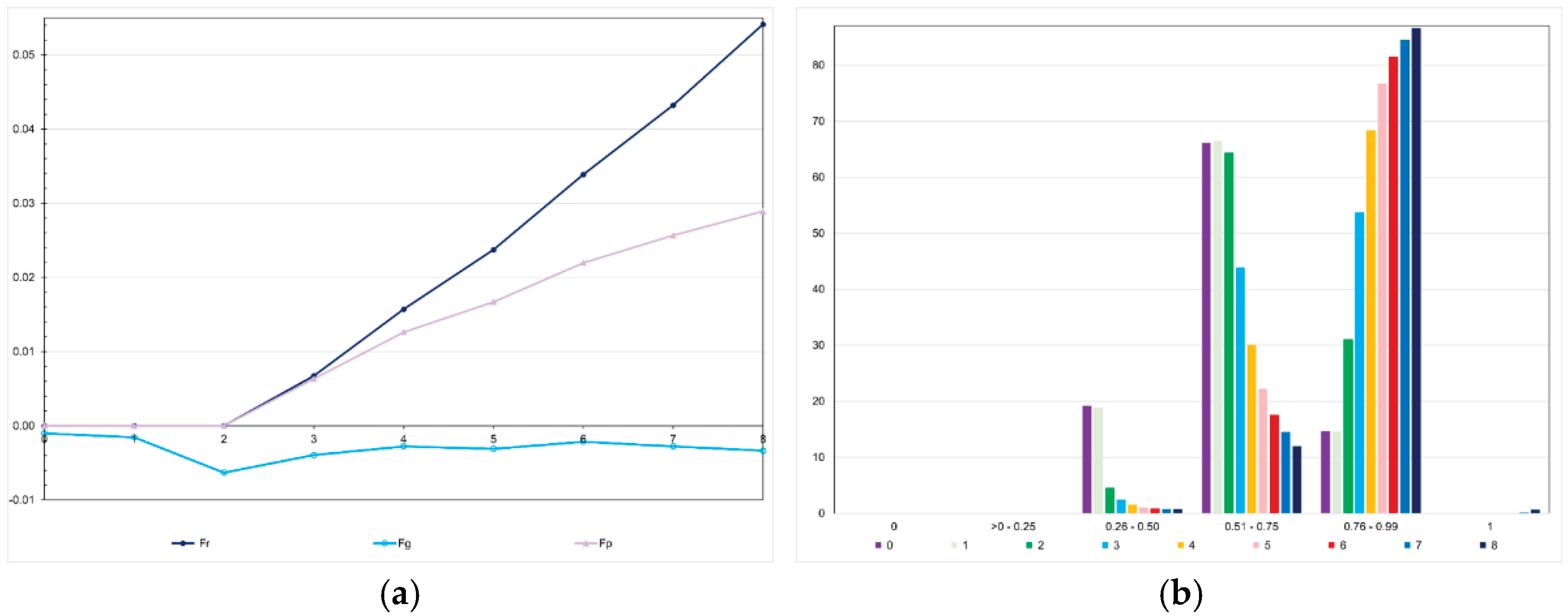
We observed, assuming genomic selection with training set including initial parents and 10% of the individuals/generation, that the realized F showed an almost perfect correlation with the expected F (0.996; generations 3 to 8) and a positive intermediate correlation with the genomic F (0.435) (Figure 11). However, the realized F (Fr) was higher than the expected F (Fp) (Fr = −0.01 + 2.19Fp; r2 = 0.99). The difference was proportional to the number of selection cycles. The analysis of the favorable allele frequency changes over the selection cycles, assuming the same genomic selection procedure, showed changes from −0.37 to 0.55 (0.27 on average). In the generation 0, no favorable allele was lost or fixed. The range for the favorable allele frequency in the parents was 0.26-0.97 (0.61 on average). After seven selection cycles, the range shifted to 0.29-1.00 (0.88 on average), but only five favorable alleles were fixed (Figure 11).
4. Discussion
Our main contributions on the efficiency of recurrent genomic selection in panmictic populations are that genomic selection efficacy, expressed as realized total genetic gain, is proportional to the population LD level and that, except for dominant epistasis, epistasis negatively impacts its efficacy, compared to the efficacy under additive-dominance model. The genomic selection using parents and 20% of phenotyped individuals in each generation as the training set provided a total genetic gain in the high LD population four times higher than the gain achieved in the low LD population. In the study of Thomasen, Liu and Sorensen [7], genomic selection in the large high LD population provided a genetic gain 9.1% higher than the genetic gains in the large low LD populations. Our results demonstrate that the additive genomic relationship matrix effectively expresses the genotypic similarities between individuals, due to their genetic relationship or identity by descent for genes, if relatives, and genomic similarity or IBS for SNPs, which depends on the LD between genes and SNPs.
Assuming 50% of interacting genes, the efficacy of genomic selection was 4.1 to 46.2% lower than the efficacy under no epistasis, excepting dominant epistasis. Wientjes, Bijma, Calus, Zwaan, Vitezica and van den Heuvel [6] also observed that epistasis negatively affected the accumulated genetic gains. The decrease compared to the additive model was approximately 27% for GBLUP, but only approximately 1% from including dominance. They also observed lower changes in the allele frequencies over 50 generations under epistasis, relative to the additive model. Compared with the additive value prediction accuracy under no epistasis, in 91% of our cases (seven generations x eight epistasis scenarios) the additive value prediction accuracy was lower under digenic epistasis, even for dominant epistasis. The additive value prediction accuracy under epistasis ranged from −35.5 to 1.8% relative to the accuracies assuming no epistasis.
After seven selection cycles based on genomic selection using parents and 10% of phenotyped individuals, the accumulated genetic gains for FCR in the high LD population were −30.4 and −25.4%, on average, assuming no epistasis and digenic epistasis, respectively. Thus, the absolute average rates of genetic gain were 4.3 and 3.6%, respectively. The maximum average rates of genetic gains observed in previous investigations using simulated data ranged from 0.5 to 2.6%, proportional to the trait heritability [4,5,6,7,21]. It is important to emphasize that this genomic selection procedure, which minimizes cost, led to a non-significant increase in both expected and genomic inbreeding coefficients. The low F values observed after seven genomic selection cycles – 0.03 to 0.07 – are mainly due to the avoidance of sib crosses. The genomic F values were 10 times lower. We also observed that, except for genomic selection under high selection intensity, the genomic selection procedures provided high numbers of selected progenies (low average number of selected full-sibs), in both additive-dominance and additive-dominance with epistasis models, regardless of the epistasis type.
Zhao, Zhang, Wang, Akdemir, Garrick, He and Wang [4] concluded that genomic mating effectively controls the rates of inbreeding accumulation in the population. Assuming heritability of 0.30, the inbreeding coefficient for the genomic matings ranged from 0.07 to 0.10 after five generations. Zheng, Zhang, Wang, Niu, Wu, Wang, Gao, Li and Xu [5] observed inbreeding coefficients in range 0.05-0.06 after seven cycles, higher for GBLUP and BayesA. In an American Angus cattle population under genomic selection over 15 years, Lozada-Soto, Maltecca, Lu, Miller, Cole and Tiezzi [11] observed an increase in the inbreeding coefficient from approximately 0.04 to 0.06. The genomic F was much higher and increased from approximately 0.25 to 0.28. Makanjuola, Miglior, Abdalla, Maltecca, Schenkel and Baes [13] also observed higher average genomic inbreeding coefficients in Holstein and Jersey cattle populations (0.31 and 0.43), relative to the average pedigree-based values (0.08 and 0.07). Over 18 years of selection, including genomic selection, the pedigree-based F increased from approximately 0.04 to 0.08-0.09 and the genomic F increased from 0.20 to 0.33 and from 0.41 to 0.43, in both populations. Low to intermediate negative and positive correlations between the expected and genomic F (−0.44 to 0.63) has been observed in several studies [11,22,23,24,25].
Regarding the impact of model updating, training set size, and selection intensity, our results agree with those obtained in studies based on simulated- and empirical-datasets. We observed that genomic selection requires model updating to achieve higher genetic gains. This is necessary because selection changes gene frequencies and, consequently, the LD between genes and SNPs, and recombination also alters the LD for genes and SNPs. Li, Zhang, Liu and Chen [8] observed that genotyping 40-50% of each litter in the previous three-four generations can provide similar selection efficacy assuming 100% of genotyping. A decrease of 50% in the phenotyping cost decreased the genomic selection efficacy by only 1.5% with no significant impact on the additive value prediction accuracy (3.4% lower on average), genotypic variance (lower decrease), and inbreeding level (12% lower). Obsteter, et al. [26] concluded that, in dairy cattle breeding, the genetic gain increased by increasing genotyping, despite reduced phenotyping. By increasing the selection intensity (decreasing by 50% the numbers of males and females selected or the effective population size), the total genetic gain increased 9.6%. Interestingly to emphasize, the additive value prediction accuracy was 2.9% lower on average, the genotypic variance in the last generation was 10.2% lower, and the inbreeding coefficient was 75% higher but the magnitude was not high (0.06).
Regarding the significance of the expected additive relationship matrix, pedigree-based BLUP can only be as efficient as genomic selection in populations with low LD level. Additionally, the genetic assessment for sex limited, difficult or expensive to measure, or post-slaughtering traits, is also more efficient by genomic selection than by pedigree-based BLUP. When there are a considerable proportion of non-measured individuals, pedigree-based BLUP is much less efficient than genomic selection (−26%) and leads to a much higher level of inbreeding (three times higher). The higher inbreeding results from a minimization of the number of selected progenies (maximization of the average number of full sibs selected). Probably because they simulated low LD dairy cattle populations, Seno, et al. [27] did not observe differences between pedigree- and genomic-based selection, regarding genetic gains and inbreeding level. Using a simulated livestock population, Wientjes, Bijma, Calus, Zwaan, Vitezica and van den Heuvel [6] concluded that genomic selection outperformed pedigree selection in terms of long-term genetic gain. Both approaches were equivalent in decreasing the genotypic variance and the decrease in heterozygosity was slightly lower for pedigree than for genomic selection. However, the relationship information has not been disregarded in animal breeding. By combining genomic and historical genetic relationship information, ssGBLUP became the most important method for genetic evaluations currently employed [28]. In the simulation-based studies of Buttgen, et al. [29] and Pocrnic, et al. [30], different long-term genotyping and selection strategies in laying hen breeding programs were assessed, including pedigree-based BLUP. Regardless of the generation interval, the rate of genetic progress was higher using genomic selection. In general, the rate of inbreeding was higher with genomic selection too.
5. Conclusions
The genomic selection efficacy, expressed as realized total genetic gain, is proportional to the LD level and genotypic variance. Only in low LD populations can pedigree-based BLUP be as efficient as genomic selection. Genomic selection requires model updating to achieve a higher efficacy. The training set size required by genomic selection can be as low as 10%/generation. Under this low-cost scenario, the genomic selection efficacy was only 5.5% lower than the maximum efficacy. There is no difference between genetic evaluation methods regarding the decrease in the genotypic variance. In general, additive value prediction accuracies and genetic gains were highly correlated. The accumulated inbreeding level under genomic selection was not high (3-7%) due to avoidance of sib cross. The genomic inbreeding coefficient over generations was close to zero, irrespective of the genetic model. The realized F was almost perfectly correlated with the expected value, but showing higher magnitude (4 to 93%), which was proportional to the selection cycle number. Except for dominant epistasis, the efficacy of genomic selection under epistasis was 4.1 to 46.2% lower than the efficacy assuming no epistasis.
Author Contributions
Conceptualization, J.M.S.V. and P.S.L.; methodology, J.M.S.V.; software, J.M.S.V.; formal analysis, J.P.A.S.; data curation, J.M.S.V.; writing—original draft preparation, J.M.S.V.; writing—review and editing, J.P.A.S. and P.S.L.; funding acquisition, J.M.S.V. All authors have read and agreed to the published version of the manuscript.
Funding
This research was funded by The National Council for Scientific and Technological Development (CNPq), the Brazilian Federal Agency for Support and Evaluation of Graduate Education (CAPES; Finance Code 001), and the Foundation for Research Support of Minas Gerais State (FAPEMIG).
Data Availability Statement
The dataset is available at https://doi.org/10.6084/m9.figshare.26866762.v1, https://doi.org/10.6084/m9.figshare.26947903.v2, https://doi.org/10.6084/m9.figshare.26951263.v1, and https://doi.org/10.6084/m9.figshare.26952103.v1.
Conflicts of Interest
The authors declare no conflicts of interest.
Abbreviations
The following abbreviations are used in this manuscript:
| F | Inbreeding coefficient |
| GS | Genomic selection |
| GV | Selection based on the true genotypic value |
| LD | Linkage disequilibrium |
| NS | No selection |
| pbB | Pedigree-based BLUP |
References
- Jones, H.; Wilson, P. Progress and opportunities through use of genomics in animal production. In TRENDS IN GENETICS, 2022; Vol. 38, pp 1228-1252.
- Misztal, I.; Lourenco, D.; Legarra, A. Current status of genomic evaluation. In Journal of animal science, 2020; Vol. 98.
- Zhang, P.; Qiu, X.; Wang, L.; Zhao, F. Progress in Genomic Mating in Domestic Animals. In ANIMALS, 2022; Vol. 12.
- Zhao, F.; Zhang, P.; Wang, X.; Akdemir, D.; Garrick, D.; He, J.; Wang, L. Genetic gain and inbreeding from simulation of different genomic mating schemes for pig improvement. In JOURNAL OF ANIMAL SCIENCE AND BIOTECHNOLOGY, 2023; Vol. 14.
- Zheng, X.; Zhang, T.; Wang, T.; Niu, Q.; Wu, J.; Wang, Z.; Gao, H.; Li, J.; Xu, L. Long-Term Impact of Genomic Selection on Genetic Gain Using Different SNP Density. In AGRICULTURE-BASEL, 2022; Vol. 12.
- Wientjes, Y.C.J.; Bijma, P.; Calus, M.P.L.; Zwaan, B.J.; Vitezica, Z.G.; van den Heuvel, J. The long-term effects of genomic selection: 1. Response to selection, additive genetic variance, and genetic architecture. Genetics Selection Evolution 2022, 54. [CrossRef]
- Thomasen, J.R.; Liu, H.; Sorensen, A.C. Genotyping more cows increases genetic gain and reduces rate of true inbreeding in a dairy cattle breeding scheme using female reproductive technologies. Journal of dairy science 2020, 103, 597-606. [CrossRef]
- Li, X.; Zhang, Z.; Liu, X.; Chen, Y. Impact of genotyping strategy on the accuracy of genomic prediction in simulated populations of purebred swine. In ANIMAL, 2019; Vol. 13, pp 1804-1810.
- Tan, X.; Liu, R.; Li, W.; Zheng, M.; Zhu, D.; Liu, D.; Feng, F.; Li, Q.; Liu, L.; Wen, J., et al. Assessment the effect of genomic selection and detection of selective signature in broilers. Poult Sci 2022, 101, 101856. [CrossRef]
- Mancin, E.; Tuliozi, B.; Sartori, C.; Guzzo, N.; Mantovani, R. Genomic Prediction in Local Breeds: The Rendena Cattle as a Case Study. In ANIMALS, 2021; Vol. 11.
- Lozada-Soto, E.; Maltecca, C.; Lu, D.; Miller, S.; Cole, J.; Tiezzi, F. Trends in genetic diversity and the effect of inbreeding in American Angus cattle under genomic selection. In GENETICS SELECTION EVOLUTION, 2021; Vol. 53.
- Hollifield, M.; Lourenco, D.; Bermann, M.; Howard, J.; Misztal, I. Determining the stability of accuracy of genomic estimated breeding values in future generations in commercial pig populations. In Journal of animal science, 2021; Vol. 99.
- Makanjuola, B.; Miglior, F.; Abdalla, E.; Maltecca, C.; Schenkel, F.; Baes, C. Effect of genomic selection on rate of inbreeding and coancestry and effective population size of Holstein and Jersey cattle populations. In Journal of dairy science, 2020; Vol. 103, pp 5183-5199.
- Cuyabano, B.; Wackel, H.; Shin, D.; Gondro, C. A study of Genomic Prediction across Generations of Two Korean Pig Populations. In ANIMALS, 2019; Vol. 9.
- Kempthorne, O. The theoretical values of correlations between relatives in random mating populations. Genetics 1954, 40, 153-167.
- Covarrubias-Pazaran, G. Genome-Assisted Prediction of Quantitative Traits Using the R Package sommer. PloS one 2016, 11. [CrossRef]
- VanRaden, P.M. Efficient methods to compute genomic predictions. Journal of dairy science 2008, 91, 4414-4423. [CrossRef]
- Su, G.; Christensen, O.F.; Ostersen, T.; Henryon, M.; Lund, M.S. Estimating additive and non-additive genetic variances and predicting genetic merits using genome-wide dense single nucleotide polymorphism markers. PloS one 2012, 7, e45293. [CrossRef]
- Amadeu, R.R.; Cellon, C.; Olmstead, J.W.; Garcia, A.A.; Resende, M.F.; Munoz, P.R. AGHmatrix: R Package to Construct Relationship Matrices for Autotetraploid and Diploid Species: A Blueberry Example. Plant Genome 2016, 9. [CrossRef]
- Vazquez, A.I.; Bates, D.M.; Rosa, G.J.; Gianola, D.; Weigel, K.A. Technical note: an R package for fitting generalized linear mixed models in animal breeding. Journal of animal science 2010, 88, 497-504. [CrossRef]
- Gore, D.; Okeno, T.; Muasya, T.; Mburu, J. Improved response to selection in dairy goat breeding programme through reproductive technology and genomic selection in the tropics. In SMALL RUMINANT RESEARCH, 2021; Vol. 200.
- Nishio, M.; Inoue, K.; Ogawa, S.; Ichinoseki, K.; Arakawa, A.; Fukuzawa, Y.; Okamura, T.; Kobayashi, E.; Taniguchi, M.; Oe, M., et al. Comparing pedigree and genomic inbreeding coefficients, and inbreeding depression of reproductive traits in Japanese Black cattle. BMC genomics 2023, 24, 376. [CrossRef]
- Caballero, A.; Fernandez, A.; Villanueva, B.; Toro, M.A. A comparison of marker-based estimators of inbreeding and inbreeding depression. Genetics, selection, evolution : GSE 2022, 54, 82. [CrossRef]
- Schaeler, J.; Kruger, B.; Thaller, G.; Hinrichs, D. Comparison of ancestral, partial, and genomic inbreeding in a local pig breed to achieve genetic diversity. In CONSERVATION GENETICS RESOURCES, 2020; Vol. 12, pp 77-86.
- Makanjuola, B.; Maltecca, C.; Miglior, F.; Schenkel, F.; Baes, C. Effect of recent and ancient inbreeding on production and fertility traits in Canadian Holsteins. In BMC genomics, 2020; Vol. 21.
- Obsteter, J.; Jenko, J.; Gorjanc, G. Genomic Selection for Any Dairy Breeding Program via Optimized Investment in Phenotyping and Genotyping. Frontiers in Genetics 2021, 12, 637017. [CrossRef]
- Seno, L.D.; Guidolin, D.G.F.; Aspilcueta-Borquis, R.R.; do Nascimento, G.B.; da Silva, T.B.R.; de Oliveira, H.N.; Munari, D.P. Genomic selection in dairy cattle simulated populations. Journal of Dairy Research 2018, 85, 125-132. [CrossRef]
- Bermann, M.; Cesarani, A.; Misztal, I.; Lourenco, D. Past, present, and future developments in single-step genomic models. Italian Journal of Animal Science 2022, 21, 673-685. [CrossRef]
- Buttgen, L.; Simianer, H.; Pook, T. Analysis of different genotyping and selection strategies in laying hen breeding programs. Genetics, selection, evolution : GSE 2025, 57, 18. [CrossRef]
- Pocrnic, I.; Obsteter, J.; Gaynor, R.C.; Wolc, A.; Gorjanc, G. Assessment of long-term trends in genetic mean and variance after the introduction of genomic selection in layers: a simulation study. Front Genet 2023, 14, 1168212. [CrossRef]
Figure 1.
A graphical summary of the simulated scenarios (GS = genomic selection; TS = training set).
Figure 1.
A graphical summary of the simulated scenarios (GS = genomic selection; TS = training set).
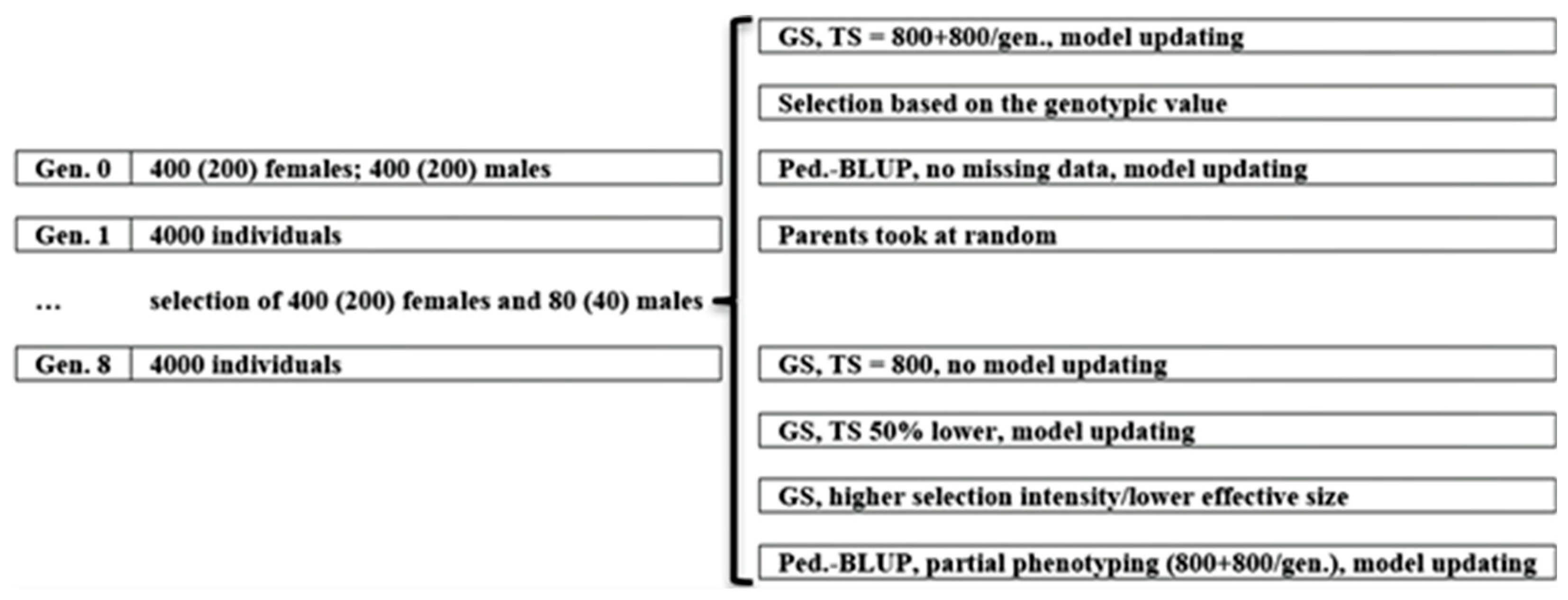
Figure 2.
Average feed conversion ratio over generations in the low (a) and high (b) LD populations under the additive-dominance model, assuming GS - genomic selection with training set including initial parents and 20% of the individuals/generation, GS1 - genomic selection with initial parents as training set, GS2 - GS with 10% of phenotyped individuals, GS3 - GS with higher selection intensity, GV - selection based on the true genotypic value, pbB - pedigree-based BLUP with phenotyping data from all individuals, pbB1 - pedigree-based BLUP with the same training set as GS, and NS - no selection. The ranges for the standard deviation for the generation means were 0.02-0.03 (0.02 on average) and 0.02-0.11 (0.07 on average), for the low- and high-LD populations.
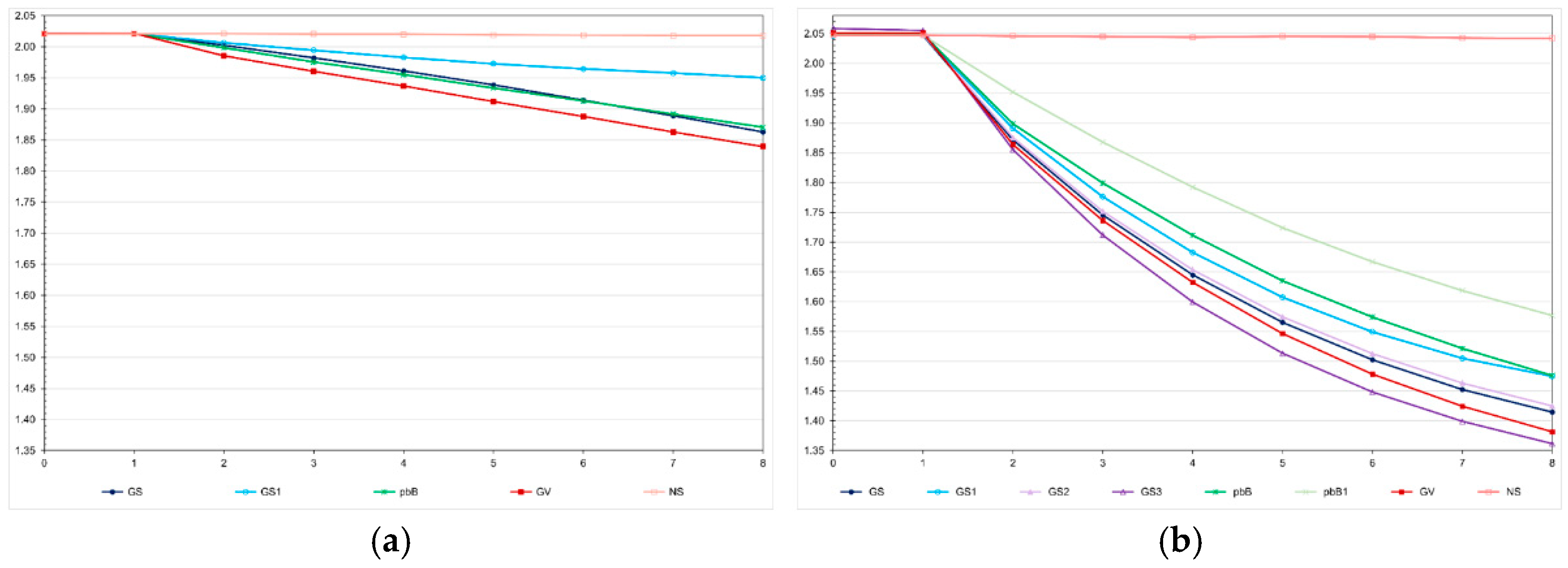
Figure 3.
Average genotypic variances for feed conversion ratio over generations in the low (a) and high (b) LD populations, under the additive-dominance model, assuming GS - genomic selection with training set including initial parents and 20% of the individuals/generation, GS1 - genomic selection with initial parents as training set, GS2 - GS with 10% of phenotyped individuals, GS3 - GS with higher selection intensity, GV - selection based on the true genotypic value, pbB - pedigree-based BLUP with phenotyping data from all individuals, pbB1 - pedigree-based BLUP with the same training set as GS, and NS - no selection. The ranges for the standard deviation for the genotypic variances were 0.00001-0.00007 (0.00003 on average) and 0.0000-0.0018 (0.00039 on average), for the low- and high-LD populations.
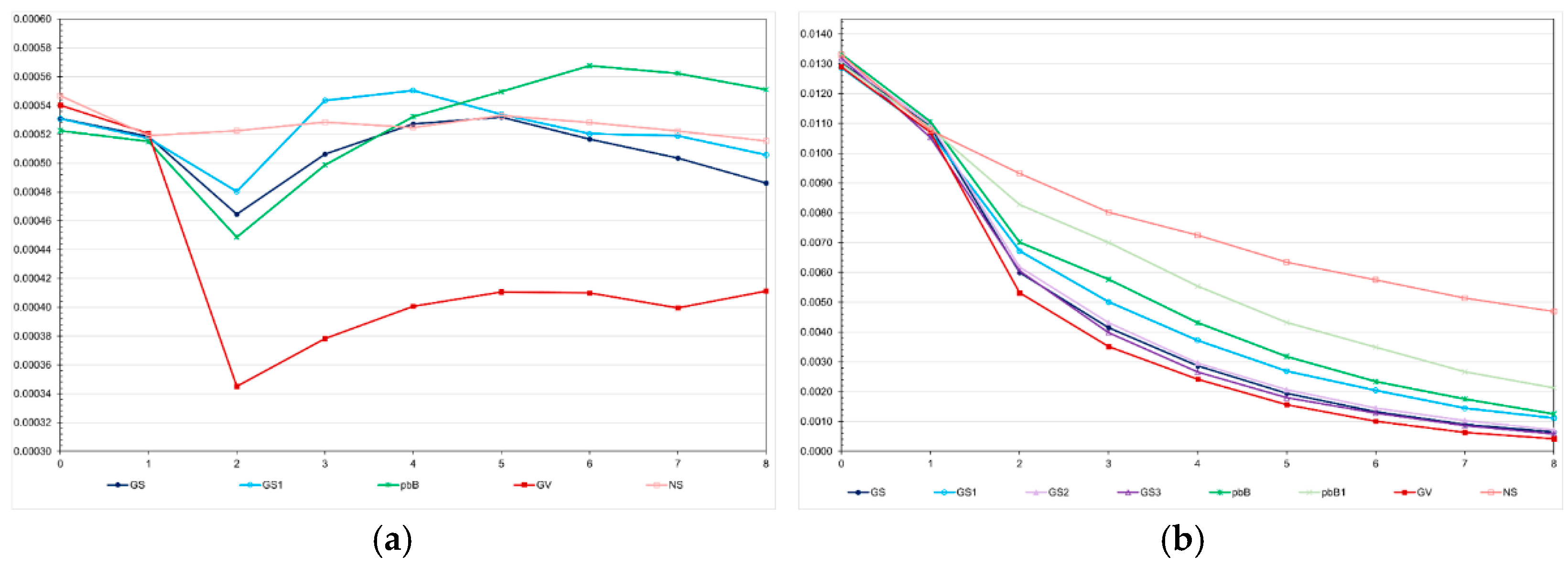
Figure 4.
Average additive value prediction accuracy for feed conversion ratio over generations in the low (a) and high (b) LD populations, under the additive-dominance model, assuming GS - genomic selection with training set including initial parents and 20% of the individuals/generation, GS1 - genomic selection with initial parents as training set, GS2 - GS with 10% of phenotyped individuals, GS3 - GS with higher selection intensity, pbB - pedigree-based BLUP with phenotyping data from all individuals, pbB1 - pedigree-based BLUP with the same training set as GS, and PS - phenotypic selection. The ranges for the standard deviation for the prediction accuracies were 0.01-0.05 (0.03 on average) and 0.01-0.07 (0.02 on average), for the low- and high-LD populations.
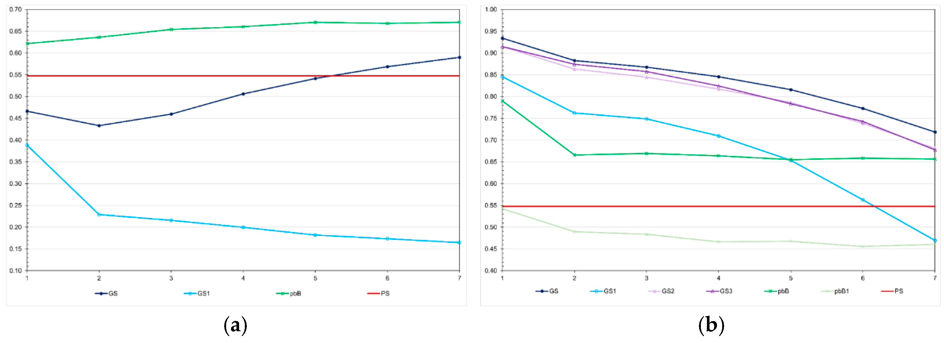
Figure 5.
Average inbreeding coefficient over generations in the low (a) and high (b) LD populations, under the additive-dominance model, assuming GS - genomic selection with training set including initial parents and 20% of the individuals/generation, GS1 - genomic selection with initial parents as training set, GS2 - GS with 10% of phenotyped individuals, GS3 - GS with 20% of phenotyped individuals and higher selection intensity, GV - selection based on the true genotypic value, pbB - pedigree-based BLUP with phenotyping data from all individuals, pbB1 - pedigree-based BLUP with the same training set as GS, and NS - no selection. The ranges for the standard deviation for the inbreeding coefficients were 0.01-0.05 (0.03 on average) and 0.01-0.07 (0.03 on average), for the low- and high-LD populations.
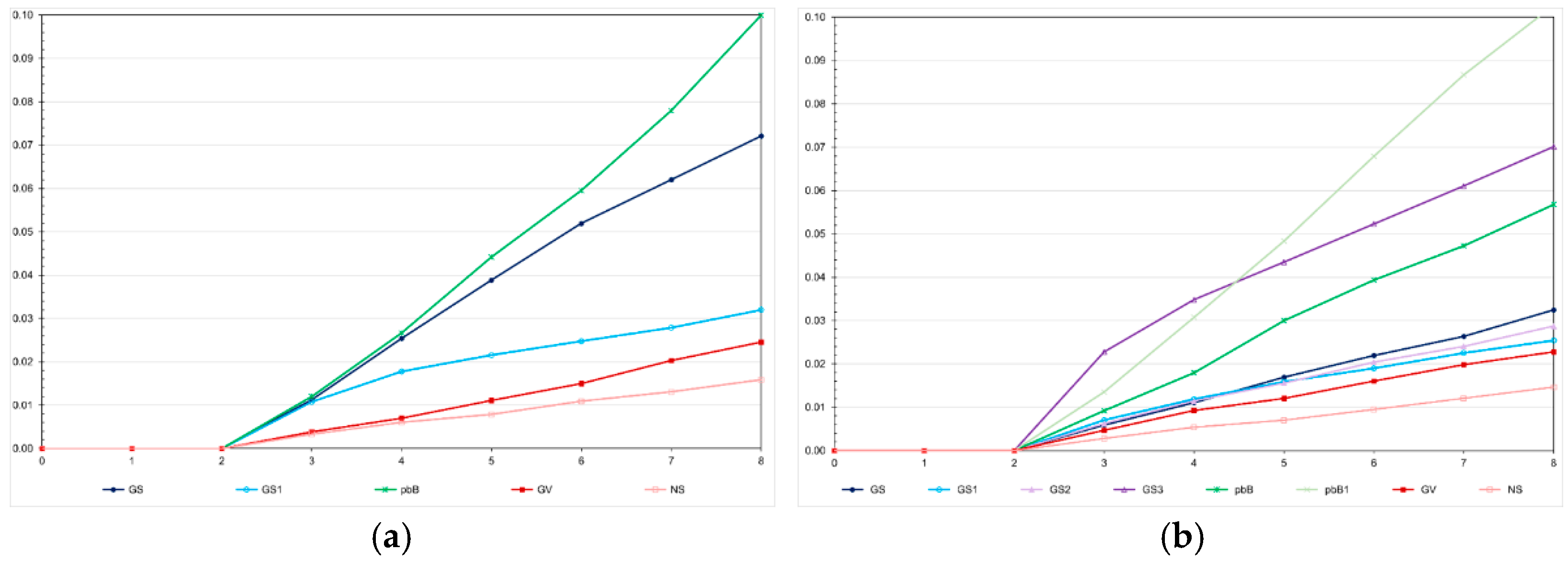
Figure 6.
Average number of progenies with selected individuals over generations in the low (a) and high (b) LD populations, under the additive-dominance model, assuming GS - genomic selection with training set including initial parents and 20% of the individuals/generation, GS1 - genomic selection with initial parents as training set, GS2 - GS with 10% of phenotyped individuals, GS3 - GS with 20% of phenotyped individuals and higher selection intensity, GV - selection based on the true genotypic value, pbB - pedigree-based BLUP with phenotyping data from all individuals, pbB1 - pedigree-based BLUP with the same training set as GS, and NS - no selection. The ranges for the standard deviation for the number of progenies were 4-80 (9.5 on average) and 3-23 (7.6 on average), for the low- and high-LD populations.
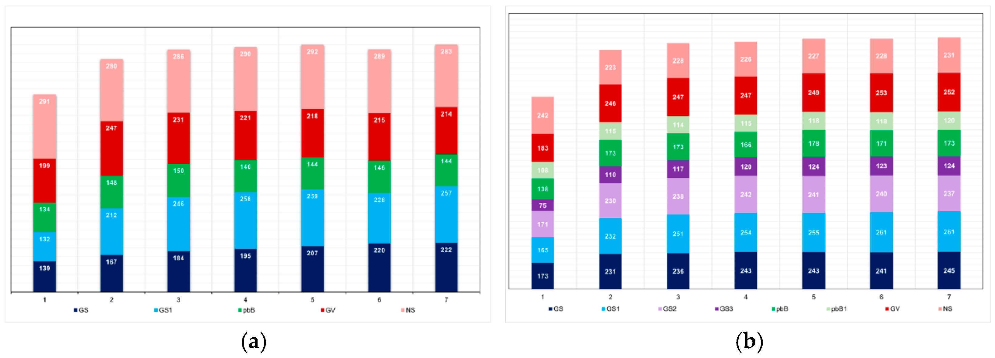
Figure 7.
Average genomic inbreeding coefficient over generations in the low (a) and high (b) LD populations, under the additive-dominance model, assuming GS - genomic selection with training set including initial parents and 20% of the individuals/generation, GS1 - genomic selection with initial parents as training set, GS2 - GS with 10% of phenotyped individuals, and GS3 - GS with 20% of phenotyped individuals and higher selection intensity. The ranges for the standard deviation for the genomic inbreeding coefficients were 0.02-0.08 (0.04 on average) and 0.04-0.09 (0.06 on average), for the low- and high-LD populations.
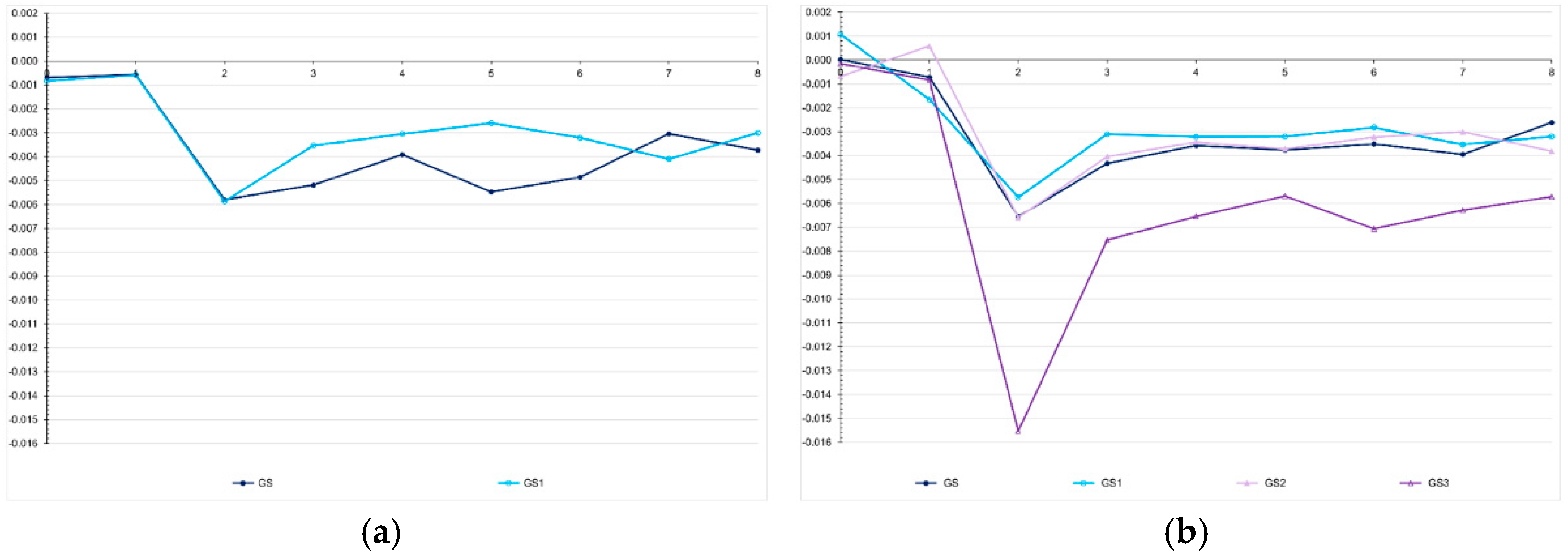
Figure 8.
Average feed conversion ratio (a) and genotypic variance (b) over generations in the high LD population, assuming seven types of epistasis and an admixture of types (E1 = complementary; E2 = duplicate; E3 = dominant; E4 = recessive; E5 = dominant and recessive; E6 = duplicate genes with cumulative effects; E7 = non-epistatic gene interaction; and E8 = all types), and GS - genomic selection with training set including initial parents and 10% of the individuals/generation. The ranges for the standard deviation for the generation means and genotypic variances were 0.02-0.13 (0.06 on average) and 0.000-0.001 (0.0003 on average), respectively.
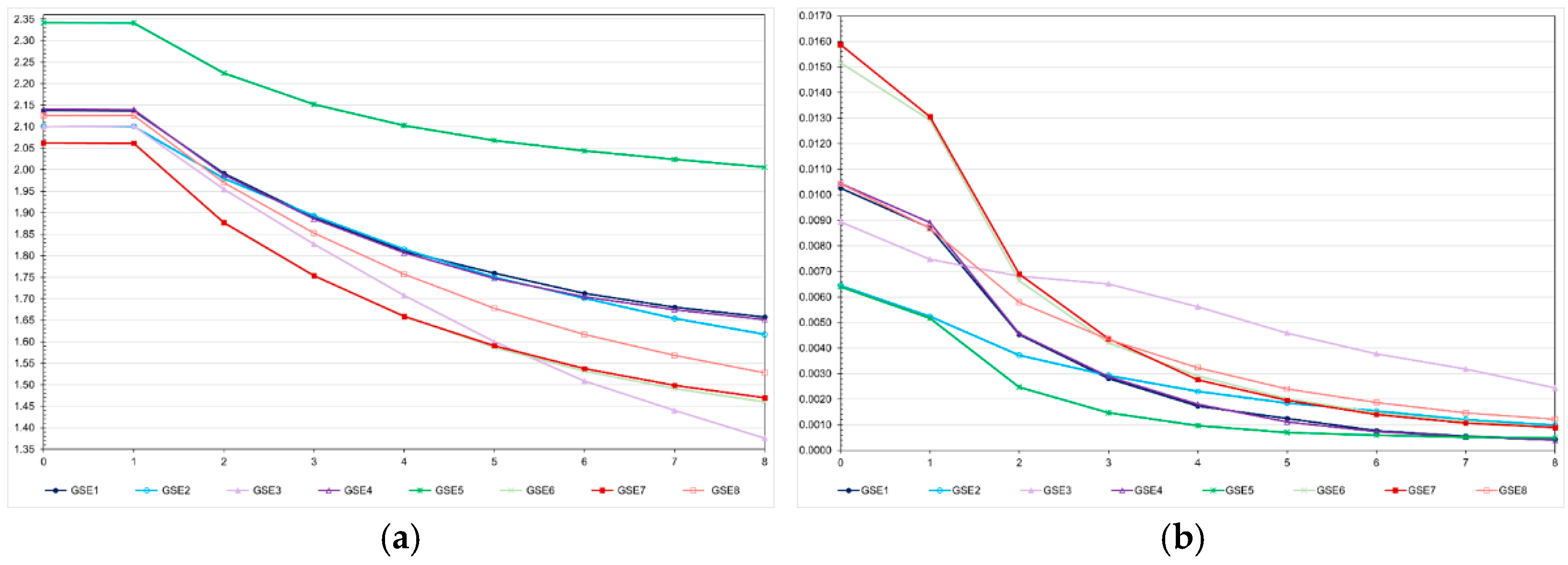
Figure 9.
Average additive value prediction accuracy for feed conversion ratio (a) and inbreeding coefficient (b) over generations in the high LD population, assuming seven types of epistasis and an admixture of types (E1 = complementary; E2 = duplicate; E3 = dominant; E4 = recessive; E5 = dominant and recessive; E6 = duplicate genes with cumulative effects; E7 = non-epistatic gene interaction; and E8 = all types), GS - genomic selection with training set including initial parents and 10% of the individuals/generation, and PS – phenotypic selection. The ranges for the standard deviation for the prediction accuracies and inbreeding coefficients were 0.01-0.06 (0.03 on average) and 0.021-0.025 (0.023 on average), respectively.
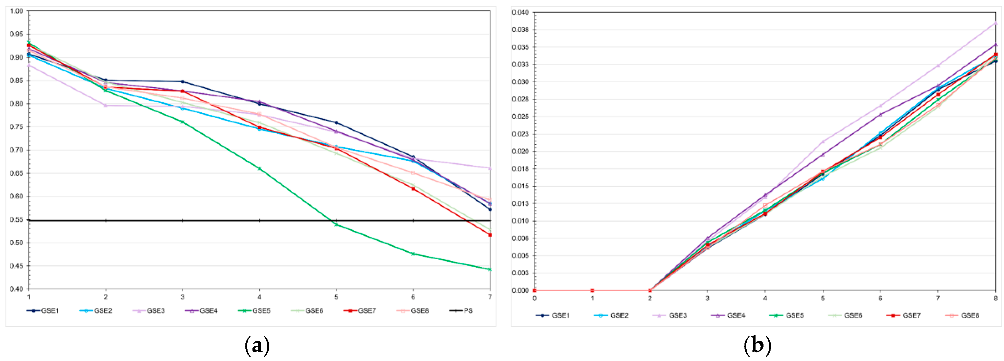
Figure 10.
Average genomic inbreeding coefficient (a) and number of progenies with selected individuals over generations in the high LD population (b), assuming seven types of epistasis and an admixture of types (E1 = complementary; E2 = duplicate; E3 = dominant; E4 = recessive; E5 = dominant and recessive; E6 = duplicate genes with cumulative effects; E7 = non-epistatic gene interaction; and E8 = all types), and GS - genomic selection with training set including initial parents and 10% of the individuals/generation. The ranges for the standard deviation for the genomic inbreeding coefficients and number of progenies were 0.04-0.09 (0.06 on average) and 5-13 (9 on average), respectively.
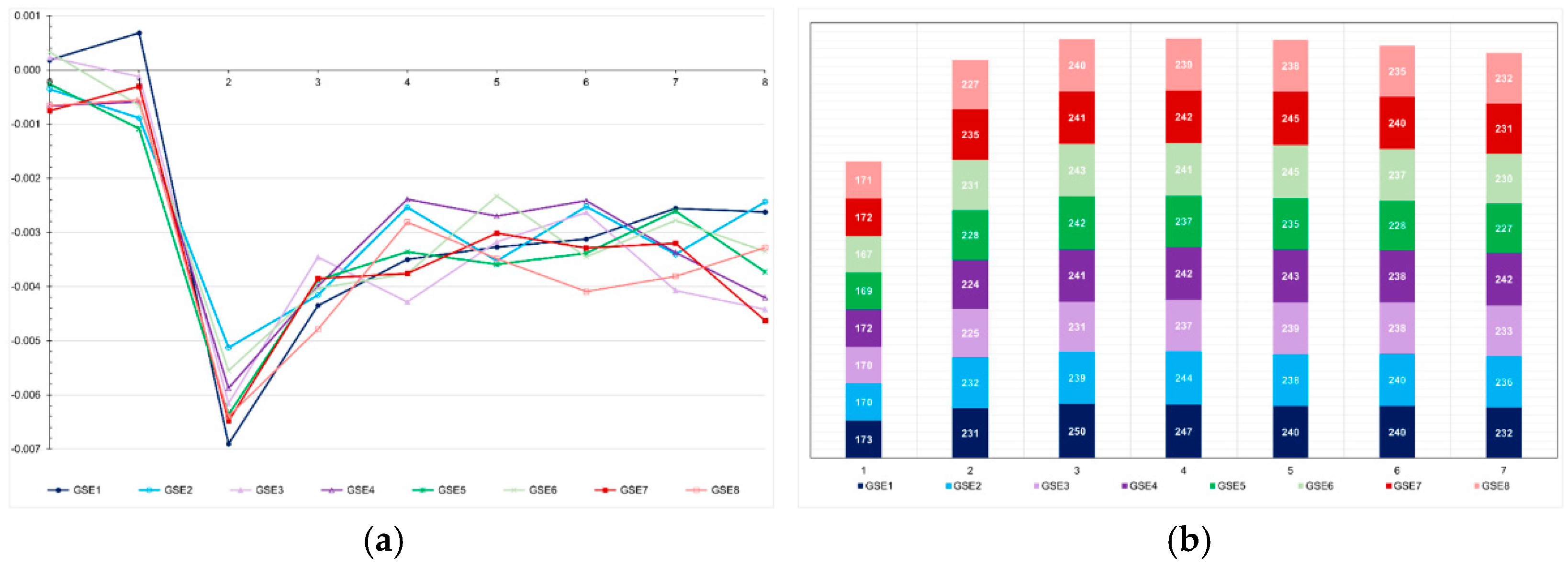
Figure 11.
Average expected- (p), genomic- (g) and realized (r) inbreeding coefficients (a) and distribution of frequencies for the favorable alleles over generations in the high LD population (b), under the additive-dominance model, assuming genomic selection with training set including initial parents and 10% of the individuals/generation.
Disclaimer/Publisher’s Note: The statements, opinions and data contained in all publications are solely those of the individual author(s) and contributor(s) and not of MDPI and/or the editor(s). MDPI and/or the editor(s) disclaim responsibility for any injury to people or property resulting from any ideas, methods, instructions or products referred to in the content. |
© 2025 by the authors. Licensee MDPI, Basel, Switzerland. This article is an open access article distributed under the terms and conditions of the Creative Commons Attribution (CC BY) license (http://creativecommons.org/licenses/by/4.0/).
Copyright: This open access article is published under a Creative Commons CC BY 4.0 license, which permit the free download, distribution, and reuse, provided that the author and preprint are cited in any reuse.


