
Submitted:
21 August 2025
Posted:
22 August 2025
You are already at the latest version
Abstract
When applying maximum likelihood estimation to the infinite mixture distributions, closed-form expressions for the parameters are rarely obtainable, so numerical methods, such as the Newton–Raphson technique, are often employed. A primary challenge in numerical methods is selecting suitable initial values. In this paper, the bootstrap approach is applied to determine initial parameter values for maximum likelihood estimation in the infinite mixture distributions. The bootstrap method is employed to generate the mixing distribution. The parameter estimates of the mixing distribution are used as initial values for performing maximum likelihood estimation on the infinite mixture distributions. In this study, both nonparametric and parametric bootstrap approaches are applied. Monte Carlo simulations are used to assess the performance of both bootstrap approaches. Simulation results indicate that the method of moments and the two bootstrap-based approaches yield identical maximum likelihood estimators. The study also reveals that when raw moments are unavailable or undefined, both bootstrap-based methods, especially the nonparametric bootstrap, offer a reliable means of determining initial values. The proposed method showed good performance when applied on the third-party liability claims data in Indonesia.
Keywords:
infinite mixture distribution
; bootstrap
; maximum likelihood estimation
; Newton-Raphson method
; mixing distribution
1. Introduction
An infinite mixture distribution is an extension of the finite mixture model where the number of components is not fixed in advance and can, in principle, be countably infinite. Instead of a finite sum of distributions, the mixture becomes an infinite sum or an integral over a space of possible parameters (Klugman et al., 2019). In actuarial science, the infinite mixture distributions are used in credibility theory and bonus malus systems to model claim frequency and claim severity (Herzog, 2010; Lemaire, 1995). The infinite mixture distributions have advantages over standard distributions, namely being able to capture complex data structures and data with high heterogeneity. Such data are typically multimodal, skewed, or heavy-tailed in the case of continuous data (Ghosal & van der Vaart, 2001), and the variance of the data is larger than expected by standard distribution models, especially the Poisson model (Canale & Prünster, 2017; Wade & Ghahramani, 2018).
Several studies have discussed distributions that are included in the infinite mixture distributions for discrete and continuous cases. Some examples of distributions that are included in discrete distributions are the Poisson-Lindley distribution (Sankaran, 1970); the Poisson-lognormal distribution (Bulmer, 1974); the Poisson-gamma distribution, the Poisson-inverse Gaussian distribution, the Poisson-generalized inverse Gaussian distribution, the Poisson-beta distribution, the Poisson-uniform distribution (G. Willmot, 1986; G. E. Willmot, 1987); the negative binomial-Lindley distribution (Zamani, 2010); the Poisson-weighted Lindley distribution (Abd El-Monsef & Sohsah, 2014); the Poisson-Sujatha distribution (Shanker, 2016b); the Poisson-Amarendra distribution (Shanker, 2016a); the Poisson-Aradhana distribution (Shanker, 2017); the New Poisson mixed weighted Lindley distribution (Atikankul et al., 2020). Some examples of distributions that are included in continuous distributions are the inverse exponential-gamma distribution (Anantasopon et al., 2015), the lognormal-gamma distribution (Moumeesri et al., 2020), the exponential-gamma distribution (McNulty, 2021), and the Rayleigh-Rayleigh distribution (Jaroengeratikun et al., 2022).
The Maximum likelihood estimation method of the parameters of the infinite mixture distributions often requires using numerical methods such as the Newton-Raphson method because no analytical solution is obtained. The problem in the Newton-Raphson method is determining the initial values. In several studies (Anantasopon et al., 2015; McNulty, 2021; Moumeesri et al., 2020; G. Willmot, 1986), determining the initial parameter values for the maximum likelihood estimator (MLE) is not mentioned or recommended even though it is a very important step. Some studies use other parameter estimation methods as initial values, for example the method of moments (Abd El-Monsef & Sohsah, 2014; Jaroengeratikun et al., 2022; Sankaran, 1970; Shanker, 2016b, 2016a, 2017). However, sometimes the use of the moment method does not provide an analytical solution (Atikankul et al., 2020; Zamani, 2010). Therefore, a method is needed to determine the initial parameter values for the MLE of the infinite mixture distributions so the numerical method can be run.
This paper discusses determining the initial parameter values based on the bootstrap approach for the MLE of the infinite mixture distributions. The bootstrap approach is used to generate the mixing distribution. The parameter estimates from the mixing distribution are used as the initial parameter values for the MLE of the infinite mixture distributions. Both nonparametric and parametric bootstrap approaches will be used in this paper. Monte Carlo simulations are used to assess the performance of both bootstrap approaches. The Indonesian automobile insurance claims data are used to illustrate the proposed method. The rest of this paper is arranged as follows. In Section 2, the theory of the infinite mixture distributions is discussed, along with several examples of distributions. In Section 3, nonparametric and parametric bootstrap approaches are proposed as ways to obtain the initial parameter values for the MLE of the infinite mixture distributions. The simulation study is conducted in Section 4. Section 5 discusses the application of the proposed method. The discussion and conclusion are presented in Section 6.
2. The Infinite Mixture Distributions
In statistics, creating new distributions can be done in various ways, and one important method is through the concept of mixing. Mixing is the process of forming a new distribution by combining two or more distributions, usually by applying weights. The result of this process is called a mixture distribution. An infinite mixture distribution is a type of probability distribution created by mixing (i.e., combining) an infinite number of component distributions. An infinite mixture distribution can be written as:
where the integral is taken over all values of λ with positive probability, is the probability density function (pdf) or probability mass function (pmf) of the random variable conditional on , and is the pdf of the random variable Λ known as the mixing distribution (Klugman et al., 2019). The distribution function can be determined from
Moments of the infinite mixture distribution can be found from
and, in particular,
In this section, we discuss 3 distributions that include in the infinite mixture distributions, namely the Poisson-Lindley distribution (Sankaran, 1970), the Inverse exponential-gamma distribution (Anantasopon et al., 2015), the lognormal-gamma distribution (Moumeesri et al., 2020).
2.1. Poisson-Lindley Distribution
The Poisson–Lindley distribution is a discrete probability distribution that arises as a mixed Poisson distribution, where the Poisson parameter follows a Lindley distribution. Let be a random variable with a Poisson distribution with parameter , and the Poisson parameter follows a Lindley distribution with parameter . Then, the marginal distribution of is called the Poisson–Lindley distribution, with the pmf (Sankaran, 1970):
The Poisson–Lindley distribution is used to model automobile insurance claim frequency data to calculate the Bayesian premium (Moumeesri et al., 2020). Suppose that , , , is a random sample from the Poisson–Lindley distribution. Let , , , is a realization from the random sample. The parameter estimate of the Poisson-Lindley distribution, θ, using the method of moments is (Sankaran, 1970)
where . The parameter estimate of the Poisson-Lindley distribution, , using the maximum likelihood estimation method is the solution of the following equation (Sankaran, 1970)
Since the estimation of the parameter cannot be found in closed form, numerical method such as the Newton-Raphson method can be used to solve the above equation. The estimated parameter value through the method of moments can be used as initial value for the Newton-Raphson method.
2.2. Inverse Exponential-Gamma Distribution
Let be a random variable with an inverse exponential distribution with parameter , and the inverse exponential parameter follows a gamma distribution with parameters , and . Then, the marginal distribution of is called the inverse exponential-gamma distribution, with the pdf (Anantasopon et al., 2015)
the inverse exponential-gamma distribution is used to model motor insurance claim (Anantasopon et al., 2015). There are no -th raw moments ( is a positive integer) for this distribution (Klugman et al., 2019). The estimation of the parameters of the inverse exponential-gamma distribution, , and , using the maximum likelihood estimation method is the solution of the following two equations (Anantasopon et al., 2015)
Because closed-form solutions for the parameter estimates are unavailable, the two equations above can be solved using numerical methods, for example, the Newton–Raphson method. In Anantasopon et al. (2015), there is no proposal to use initial values for the estimated parameters of the inverse exponential-gamma distribution via the Newton-Raphson method.
2.3. Lognormal-Gamma Distribution
Let be a random variable with a lognormal distribution with parameters , and , and the lognormal parameter follows a gamma distribution with parameters , and . Then, the marginal distribution of is called the lognormal-gamma distribution, with the pdf (Moumeesri et al., 2020)
In Moumeesri et al. (2020), the lognormal-gamma distribution is used to model automobile insurance claim severity data to calculate the Bayesian premium. The log-Cauchy distribution is a special case of the lognormal-gamma distribution for with the pdf
The log-Cauchy distribution does not have defined moments. Therefore, the method of moments cannot be used to estimate the parameters of this distribution. The estimation of the parameters of the log-Cauchy distribution, and , using the maximum likelihood estimation method is the solution of the following two equations
Since closed-form expressions for the parameters do not exist, numerical approaches like the Newton–Raphson method may be applied to solve the two equations above.
3. Bootstrap-Based Initialization
In this section, a method is proposed to determine the initial parameter values for the MLE of the infinite mixture distributions using the bootstrap approach. Two bootstrap approaches, namely nonparametric and parametric bootstrap are used in this method.
Suppose that a dataset (original data) of size n, denoted as . The steps in determining the initial parameter values for the MLE of the infinite mixture distribution using the nonparametric bootstrap approach are as follows
- Randomly draw a new sample of size n with replacement from the original data to create a bootstrap sample, ;
- Calculate the estimated value of the parameter, , which in the theory of the infinite mixture distribution (Section 2) is distributed with the pdf or pmf for the bootstrap sample, denoted as ;
- Repeat steps 1-2 times to get , , , .
- Calculate the estimated values of the parameters of the mixing distribution based on the data , , , . The estimated values of these parameters become the initial parameter values for the MLE of the infinite mixture distribution.
The steps in determining the initial parameter values for the MLE of the infinite mixture distribution using the parametric bootstrap approach are as follows
- Calculate the estimated value of the parameter, , using maximum likelihood estimation method which is distributed with the pdf or pmf for the original data, denoted as ;
- Randomly draw a new sample of size n from the distribution to create a bootstrap sample, ;
- Calculate the estimated value of the parameter, , which in the theory of the infinite mixture distribution (Section 2) is distributed with the pdf or pmf for the bootstrap sample, denoted as ;
- Repeat steps 2-3 times to get , , , .
- Calculate the estimated values of the parameters of the mixing distribution based on the data , , , . The estimated values of these parameters become the initial parameter values for the MLE of the infinite mixture distribution.
4. Simulation Study
In this section, a simulation study is conducted to evaluate the performance of bootstrap-based initialization in determining the initial parameter values for the MLE of the infinite mixture distribution. The two bootstrap approaches proposed in Section 3 will be evaluated for their performance along with the method of moments. The three distributions discussed in Section 2 will be used to evaluate the performance of the proposed method. Several cases from these distributions will be applied in the simulation study. These cases are presented in Table 1. There are 9 cases of the Poisson-Lindley distribution, 18 cases of the inverse exponential gamma distribution, and 18 cases of the lognormal-gamma distribution.
The results of the simulation study of all cases in Table 1 are shown in Table 2, Table 3 and Table 4 with a simulation number of 1,000 times and B = 1,000 bootstrap replications. There are two methods for determining the initial parameter values for the MLE of the infinite mixture distributions whose performance is assessed in this simulation study, namely the method of moments (MM) and bootstrap-based methods, namely nonparametric bootstrap (NP) and parametric bootstrap (P). The performance of the two methods is assessed based on the average number of iterations and the root mean square error (RMSE) of the MLE. It is known that RMSE includes the variance and bias of the parameter estimator.
In this section, a simulation study is conducted to evaluate the performance of bootstrap-based initialization in determining the initial parameter values for the MLE of the infinite mixture distribution. The two bootstrap approaches proposed in section 3 will be evaluated for their performance along with the method of moments. The three distributions discussed in section 2 will be used to evaluate the performance of the proposed method. Several cases from these distributions will be applied in the simulation study. These cases are presented in Table 1. There are 9 cases of the Poisson-Lindley distribution, 18 cases of the inverse exponential gamma distribution, and 18 cases of the lognormal-gamma distribution.
Table 3 presents the simulation study results of the cases of the inverse exponential-gamma distribution. Only bootstrap-based methods were evaluated for their performance in the cases of the inverse exponential-gamma distribution. It can be seen that the average number of iterations is all below 30 iterations for both bootstrap-based approaches (NP, and P) and for all distribution cases. Another result is that the average number of iterations of the nonparametric bootstrap (NP) approach is less than that of the parametric bootstrap (P) approach. The difference in the results of the two approaches ranges from 2 to 12 iterations. This indicates that the nonparametric bootstrap approach has better performance than the parametric bootstrap approach as an approach in determining the initial parameter values for the MLE of the infinite mixture distributions. Another result is that all RMSE values are the same for both bootstrap-based approaches (NP, and P) and for all distribution cases. This can be concluded that bootstrap-based approaches produce the same MLE for the cases of the inverse exponential-gamma distribution.
Table 4 presents the simulation study results of the cases of the lognormal-gamma distribution. Only bootstrap-based methods were evaluated for their performance in the cases of the lognormal-gamma distribution. It can be seen that the average number of iterations is all below 25 iterations and does not differ much for both bootstrap-based approaches (NP, and P) and for all distribution cases. This shows that both bootstrap-based approaches have equally good performance as methods for determining the initial parameter values for the MLE of the infinite mixture distributions for the cases of the lognormal-gamma distribution. Another result is that all RMSE values are the same for both bootstrap-based approaches (NP, and P) and for all distribution cases. This can be concluded that bootstrap-based approaches produce the same MLE for the cases of the lognormal-gamma distribution.
5. Applications
We consider the application of the proposed method to two automobile insurance claim datasets in Indonesia for policyholders who took comprehensive coverage with expanded third-party liability in underwriting year 2019. The first dataset contains the claim frequency of the third-party liability, as presented in Table 5. The sample mean and variance for the claim frequency data are 0.00400, and 0.00402, respectively. The second dataset contains the claim severity of the third-party liability, which has 226 observations. The sample mean and standard deviation for the claim severity data are IDR 5,760,172, and IDR 7,162,913, respectively. Figure 1 shows a histogram for the claim severity data.
The Poisson-Lindley distribution will be applied to model claim frequency data of the third-party liability. Meanwhile, the inverse exponential-gamma distribution, and the lognormal-gamma distribution will be applied to model claim severity data of the third-party liability. The parameters of the three distributions will be estimated using the maximum likelihood estimation method through the Newton-Raphson numerical method with the initial values of the estimated distribution parameters determined using the bootstrap-based method proposed in this paper.
The bootstrap approach steps in Section 3 are performed on the claim frequency data of the third-party liability to obtain initial parameter estimates using both nonparametric and parametric bootstrap approaches. The results were 250.7964 and 250.5977, respectively. These initial values were used to obtain the MLE of the Poisson-Lindley distribution using the Newton-Raphson method. The results were the same for both approaches, namely 250.9390 at iteration 3. Table 5 presents claim frequency data (observed frequency) of the third-party liability, estimated probability for Poisson-Lindley distribution and expected frequency. The values in Table 5 are needed to calculate the chi-square test statistic to test the suitability of the Poisson-Lindley distribution. The result is a chi-square test statistic of 0.0120 with a p-value of 0.9128. Thus, it can be concluded that the Poisson-Lindley distribution is suitable for modeling claim frequency data of third-party liability.
Table 6 presents the results of applying the method proposed in Section 3 to claim severity data of the third-party liability as well as the results of the Kolmogorov-Smirnov test for the inverse exponential-gamma (IEG) distribution and the lognormal-gamma (LG) distribution. It can be seen that the initial parameter values of the MLE for the inverse exponential-gamma distribution are , and for the nonparametric bootstrap approach, and , and for the parametric bootstrap approach. The values of the MLE for the inverse exponential-gamma distribution are , and for both approaches. For the nonparametric bootstrap approach, it was obtained at iteration 30, while for the parametric bootstrap approach, it was obtained at iteration 54. The results for the lognormal-gamma distribution can be seen in the last column of Table 6.
The K-S test statistic values for the inverse exponential-gamma distribution and the lognormal-gamma distribution are 0.0951 and 0.0973, respectively. The critical value of the K-S test at the 1% significance level is 0.1011 (Sheskin, 2000). Thus, the inverse exponential-gamma distribution and the lognormal-gamma distribution are suitable for modeling claim severity data of the third-party liability. Figure 2 depicts the empirical cumulative distribution function (EDF) curve, the cumulative distribution function curve for the inverse exponential-gamma distribution (IEG), and the lognormal-gamma distribution (LG). It can be seen that the cumulative distribution function curve for the inverse exponential-gamma distribution is closer to the EDF. Thus, the inverse exponential-gamma distribution is more suitable for modeling claim severity data of the third-party liability than the lognormal-gamma distribution. This is supported by the smallest K-S test statistic value and the largest log-likelihood function value for the inverse exponential-gamma distribution.
6. Discussion and Conclusions
In this paper, a bootstrap-based method for determining initial values in numerical methods to obtain maximum likelihood estimators in the infinite mixture distributions is proposed. Two bootstrap approaches were used, namely nonparametric bootstrap and parametric bootstrap. Detailed steps for the two bootstrap-based approaches are outlined. This proposed method is very useful especially when faced with the problem of estimating parameters through numerical methods where there are no recommended initial values. This may occur when the moments of the distribution are not defined or there is no analytical solution for estimation using the method of moments.
In simulation study, the problem discussed is the performance assessment of the initial value determination method, not the performance of the parameter estimation method. Therefore, for further research, it is necessary to assess the performance of parameter estimation methods for distributions included in the infinite mixture distribution. The method proposed in this paper can be an alternative method for estimating distribution parameters besides existing methods. In simulation studies, we sometimes encounter situations where the iteration process of the numerical method fails to converge. This is because the method proposed in this paper is based on random data generation.
The results of the simulation study show that the method of moments and two bootstrap-based approaches produce the same maximum likelihood estimator. Another result is that when faced with the problem of no raw moments or undefined moments, two bootstrap-based approaches, especially nonparametric bootstrap, become a reliable solution as a method for determining initial values. The application of the proposed method to the third-party liability claims data for automobile insurance in Indonesia for underwriting year 2019 showed good performance.
Funding
This work was supported by the Institute for Research and Community Service, Universitas Islam Bandung, Indonesia through grant number 002/B.04/LPPM/I/2025.
Data Availability Statement
The data presented in this study are available from the author upon reasonable request.
Conflicts of Interest
The author declares no conflict of interest.
References
- Abd El-Monsef, M. M. E., & Sohsah, N. M. (2014). Poisson–Weighted Lindley Distribution. Jökull Journal, 64: 192-202. https://www.researchgate.net/publication/264122757_Poisson-Weighted_Lindley_Distribution.
- Anantasopon, S., Sattayatham, P., & Talangtam, T. (2015). The Modeling of Motor Insurance Claims with Infinite Mixture Distribution. International Journal of Applied Mathematics and Statistics, 53: 40-49. https://science.sut.ac.th/mathematics/finance/images/pdf/paper/p4-themodeling.pdf.
- Atikankul, Y., Thongteeraparp, A., & Bodhisuwan, W. (2020). The new poisson mixed weighted lindley distribution with applications to insurance claims data. Songklanakarin Journal of Science and Technology, 42: 152–162. [CrossRef]
- Bulmer, M. G. (1974). On Fitting the Poisson Lognormal Distribution to Species-Abundance Data. Biometrics, 30: 101-110. [CrossRef]
- Canale, A., & Prünster, I. (2017). Robustifying Bayesian Nonparametric Mixtures for Count Data. Biometrics, 73: 174–184. [CrossRef]
- Ghosal, S., & van der Vaart, A. W. (2001). Entropies and rates of convergence for maximum likelihood and Bayes estimation for mixtures of normal densities. The Annals of Statistics, 29: 1233-1263. [CrossRef]
- Herzog, T. N. (2010). Introduction to Credibility Theory, 4th ed. Winsted: ACTEX Publications.
- Jaroengeratikun, U., Dankunprasert, S., & Talangtam, T. (2022). Infinite Mixture of Rayleigh-Rayleigh Distribution and Its Application To Motor Insurance Claims. Pak. J. Statist., 38: 517-527. https://www.pakjs.com/wp-content/uploads/2022/07/38303.pdf.
- Klugman, S. A., Panjer, H. H., & Willmot, G. E. (2019). Loss Models: From Data to Decisions, 5th ed. New Jersey: John Wiley and Sons, Inc.
- Lemaire, J. (1995). Bonus-Malus Systems in Automobile Insurance. London: Kluwer Academic Publishers.
- McNulty, G. (2021). The Pareto-Gamma Mixture. Casualty Actuarial Society E-Forum. https://www.casact.org/sites/default/files/2023-03/McNulty_The_Pareto_Gamma_Mixture_EForum-Spring2021.pdf (Accessed on 14 August 2025).
- Moumeesri, A., Klongdee, W., & Pongsart, T. (2020). Bayesian Bonus-Malus Premium with Poisson-Lindley Distributed Claim Frequency and Lognormal-Gamma Distributed Claim Severity in Automobile Insurance. WSEAS Transactions on Mathematics, 19: 443–451. [CrossRef]
- Sankaran, M. (1970). The Discrete Poisson-Lindley Distribution. Biometrics, 26: 145-149. [CrossRef]
- Shanker, R. (2016a). The Discrete Poisson-Amarendra Distribution. International Journal of Statistical Distributions and Applications, 2: 14-21. [CrossRef]
- Shanker, R. (2016b). The Discrete Poisson-Sujatha Distribution. International Journal of Probability and Statistics, 5: 1-9. [CrossRef]
- Shanker, R. (2017). The Discrete Poisson-Aradhana Distribution. Turkiye Klinikleri Journal of Biostatistics, 9: 12–22. [CrossRef]
- Sheskin, D. J. (2000). Handbook of Parametric and Nonparametric Statistical Procedures, 2nd ed. New York: Chapman & Hall/CRC.
- Wade, S., & Ghahramani, Z. (2018). Bayesian Cluster Analysis: Point Estimation and Credible Balls (with Discussion). Bayesian Analysis, 13: 559-626. [CrossRef]
- Willmot, G. (1986). Mixed Compound Poisson Distributions. ASTIN Bulletin, 16: S59–S79. [CrossRef]
- Willmot, G. E. (1987). The Poisson-Inverse Gaussian distribution as an alternative to the negative binomial. Scandinavian Actuarial Journal, 3-4: 113–127. [CrossRef]
- Zamani. (2010). Negative Binomial-Lindley Distribution and Its Application. Journal of Mathematics and Statistics, 6: 4–9. [CrossRef]
Figure 1.
Histogram of the Claim Severity Data.
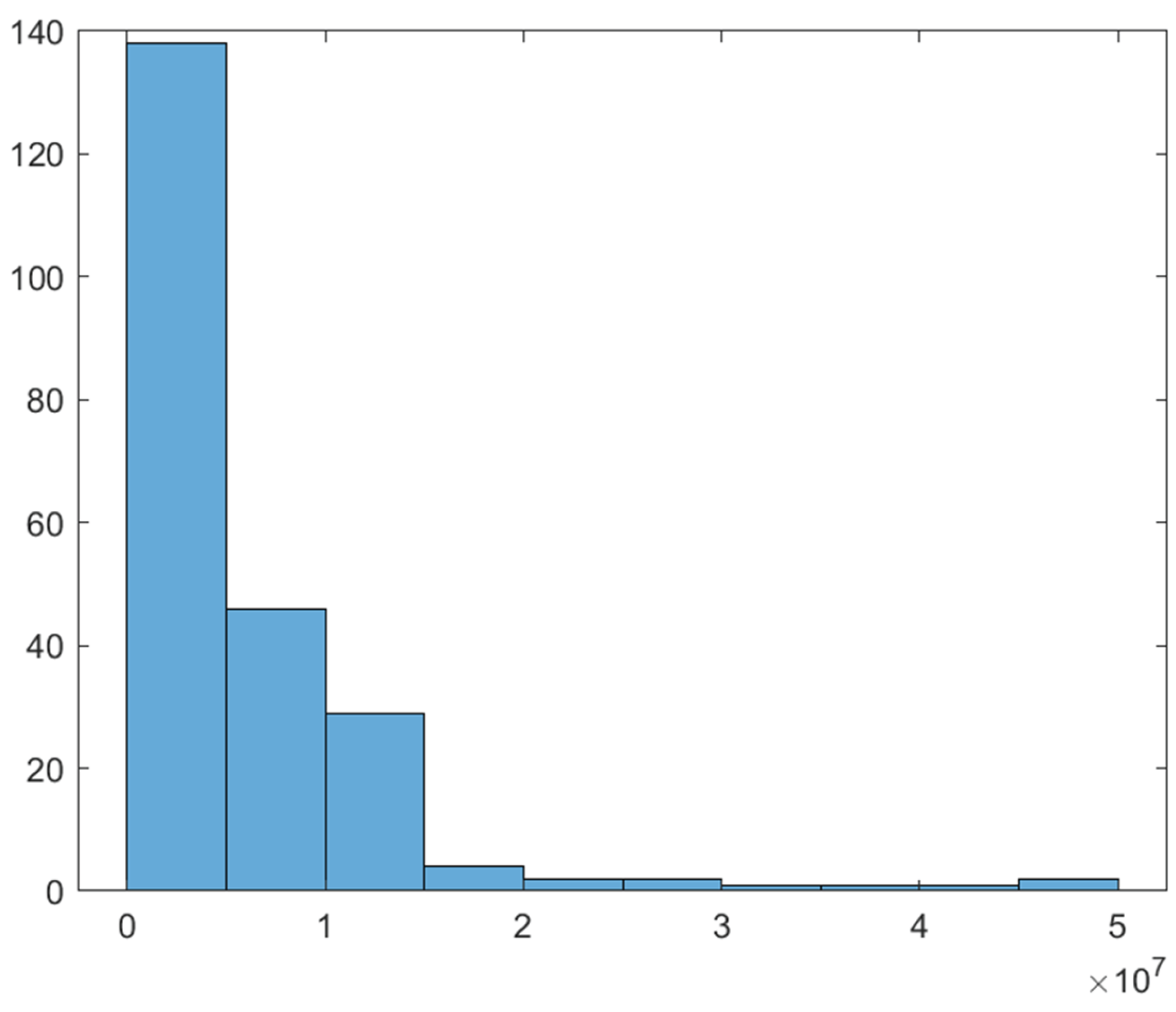
Figure 2.
The Cumulative Distribution Function.
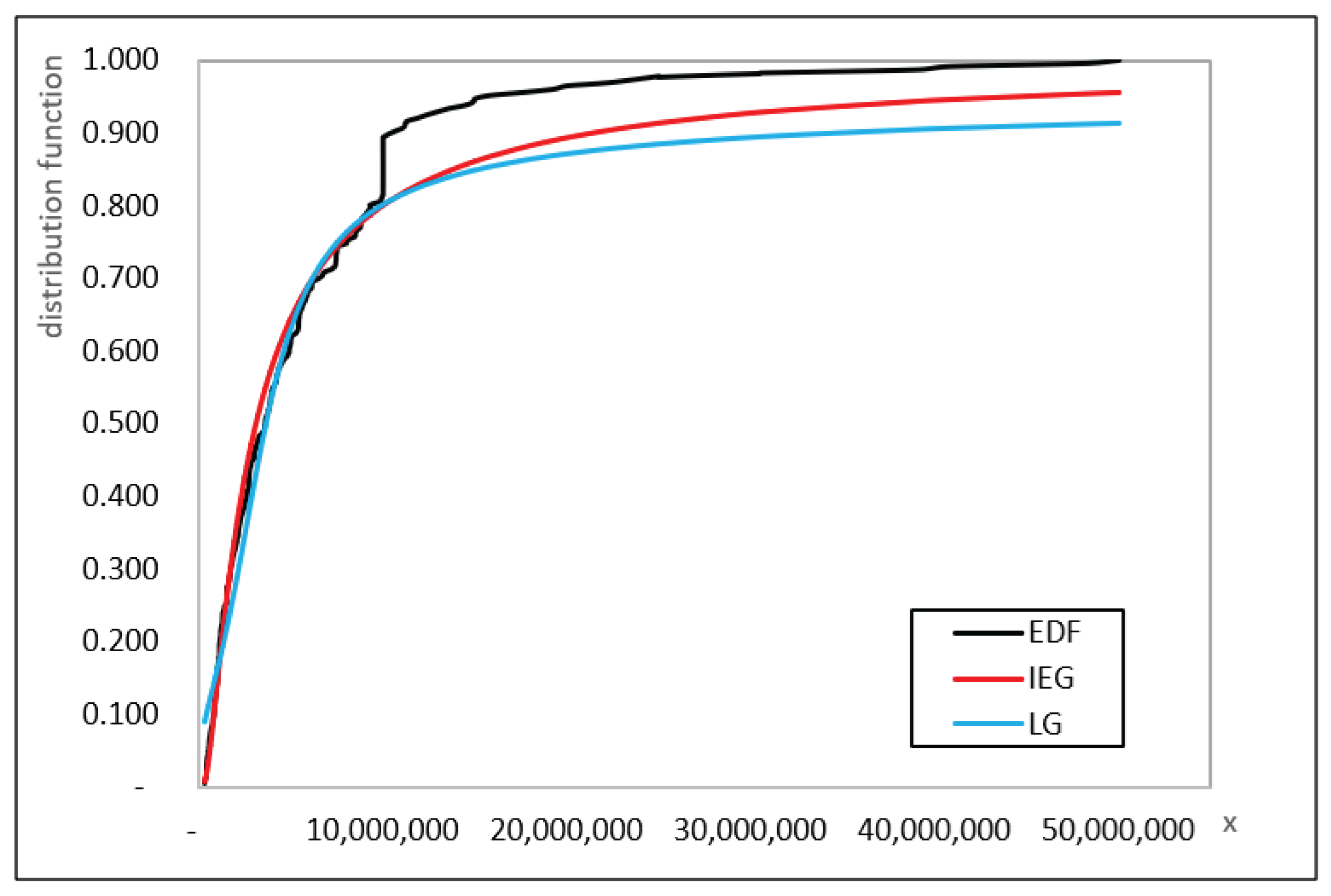

Table 1.
The Cases of The Simulation Study.
| Distributions | Parameters | Sampel Sizes |
|---|---|---|
| Poisson-Lindley | ||
| Poisson-Lindley | ||
| Poisson-Lindley | ||
| Inverse Exponential-Gamma | ||
| Inverse Exponential-Gamma | ||
| Inverse Exponential-Gamma | ||
| Inverse Exponential-Gamma | ||
| Inverse Exponential-Gamma | ||
| Inverse Exponential-Gamma | ||
| Lognormal-Gamma | ||
| Lognormal-Gamma | ||
| Lognormal-Gamma | ||
| Lognormal-Gamma | ||
| Lognormal-Gamma | ||
| Lognormal-Gamma |
Table 2.
The Simulation Study Results of The Poisson-Lindley Distribution.
| Parameter Values |
Sample Sizes |
Average Number of Iterations | RMSE | ||||
|---|---|---|---|---|---|---|---|
| MM | NP | P | MM | NP | P | ||
| 2.43 | 2.42 | 2.43 | 0.13 | 0.13 | 0.13 | ||
| 2.45 | 2.45 | 2.46 | 0.12 | 0.12 | 0.12 | ||
| 2.45 | 2.45 | 2.44 | 0.12 | 0.12 | 0.12 | ||
| 2.91 | 3.08 | 3.09 | 5.10 | 5.10 | 5.10 | ||
| 2.89 | 3.02 | 3.02 | 5.26 | 5.26 | 5.26 | ||
| 2.91 | 3.00 | 3.00 | 4.73 | 4.73 | 4.73 | ||
| 2.75 | 3.19 | 3.21 | 21.37 | 21.37 | 21.37 | ||
| 2.72 | 3.06 | 3.07 | 16.57 | 16.57 | 16.57 | ||
| 2.71 | 3.05 | 3.04 | 15.64 | 15.64 | 15.64 | ||
Table 3.
The Simulation Study Results of The Inverse Exponential-Gamma Distribution.
| Parameter Values |
Sample Sizes |
Average Number of Iterations |
||||||
|---|---|---|---|---|---|---|---|---|
| NP | P | NP | P | NP | P | |||
| 14.66 | 17.00 | 13.00 | 13.00 | 0.0040 | 0.0040 | |||
| 18.06 | 20.76 | 19.85 | 19.85 | 0.0061 | 0.0061 | |||
| 24.66 | 29.42 | 25.30 | 25.30 | 0.0080 | 0.0080 | |||
| 15.16 | 17.33 | 70.75 | 70.75 | 0.2135 | 0.2135 | |||
| 18.87 | 21.11 | 77.14 | 77.14 | 0.2315 | 0.2315 | |||
| 24.63 | 28.42 | 38.06 | 38.06 | 0.1103 | 0.1103 | |||
| 15.15 | 17.12 | 85.09 | 85.09 | 2.5479 | 2.5479 | |||
| 18.20 | 21.15 | 76.20 | 76.20 | 2.3787 | 2.3787 | |||
| 24.46 | 29.63 | 37.84 | 37.84 | 1.1732 | 1.1732 | |||
| 14.92 | 23.86 | 0.12 | 0.12 | 0.0060 | 0.0060 | |||
| 16.07 | 26.13 | 0.08 | 0.08 | 0.0040 | 0.0040 | |||
| 17.88 | 29.59 | 0.04 | 0.04 | 0.0020 | 0.0020 | |||
| 14.66 | 17.00 | 0.67 | 0.67 | 0.0140 | 0.0140 | |||
| 18.06 | 20.76 | 0.19 | 0.19 | 0.0034 | 0.0034 | |||
| 24.66 | 29.42 | 0.11 | 0.11 | 0.0020 | 0.0020 | |||
| 15.16 | 17.33 | 72.58 | 72.58 | 0.3380 | 0.3380 | |||
| 18.87 | 21.11 | 45.00 | 45.00 | 0.2161 | 0.2161 | |||
| 24.63 | 28.42 | 3.76 | 3.76 | 0.0151 | 0.0151 | |||
Table 4.
The Simulation Study Results of The Lognormal-Gamma Distribution.
| Parameter Values |
Sample Sizes |
Average Number of Iterations |
|||||
|---|---|---|---|---|---|---|---|
| NP | P | NP | P | NP | P | ||
| 20.55 | 20.61 | 237.38 | 237.38 | 2.33 | 2.33 | ||
| 19.58 | 19.67 | 262.92 | 262.92 | 1.68 | 1.68 | ||
| 18.13 | 18.14 | 179.98 | 179.98 | 1.06 | 1.06 | ||
| 21.68 | 21.75 | 228.84 | 228.84 | 2.90 | 2.90 | ||
| 20.44 | 20.52 | 310.00 | 310.00 | 2.11 | 2.11 | ||
| 19.03 | 19.06 | 327.97 | 327.97 | 1.11 | 1.11 | ||
| 22.57 | 22.70 | 353.04 | 353.04 | 3.84 | 3.84 | ||
| 21.39 | 21.42 | 286.52 | 286.52 | 2.29 | 2.29 | ||
| 20.15 | 20.15 | 235.53 | 235.53 | 1.30 | 1.30 | ||
| 22.16 | 22.24 | 281.04 | 281.04 | 3.17 | 3.17 | ||
| 20.89 | 20.91 | 297.47 | 297.47 | 2.09 | 2.09 | ||
| 19.72 | 19.73 | 304.59 | 304.59 | 1.40 | 1.40 | ||
| 22.32 | 22.42 | 369.65 | 369.65 | 2.99 | 2.99 | ||
| 20.96 | 21.02 | 407.46 | 407.46 | 2.76 | 2.76 | ||
| 19.88 | 19.91 | 235.30 | 235.30 | 1.21 | 1.21 | ||
| 22.07 | 22.19 | 261.48 | 261.48 | 3.03 | 3.03 | ||
| 21.07 | 21.12 | 247.92 | 247.92 | 2.26 | 2.26 | ||
| 19.58 | 19.60 | 288.38 | 288.38 | 1.19 | 1.19 | ||
Table 5.
Chi-Square Calculation for Claim Frequency Data.
| Number of Claims |
Observed Frequency |
Estimated Probability |
Expected Frequency |
|---|---|---|---|
| 0 | 56,263 | 0.996015 | 56262.9006 |
| 1 | 224 | 0.003969 | 224.2024 |
| 2 | 1 | 0.000016 | 0.8970 |
Table 6.
Calculation Results for Claim Severity Data.
| IEG Distribution | LG Distribution | ||
|---|---|---|---|
| Number of Observations | 226 | 226 | |
| Nonparametric Bootstrap Approach |
Initial Values |
; |
; |
| Estimated MLE Parameters |
; |
; |
|
| Number of Iterations |
30 | 17 | |
| Parametric Bootstrap Approach |
Initial Values |
; |
; |
| Estimated MLE Parameters |
; |
; |
|
| Number of Iterations |
54 | 17 | |
| Log-likelihood | -3743.2240 | -3784.0803 | |
| Test Statistic of Kolmogorov-Smirnov Test |
0.0951 | 0.0973 | |
| Critical values | 0.1011 | 0.1011 | |
Disclaimer/Publisher’s Note: The statements, opinions and data contained in all publications are solely those of the individual author(s) and contributor(s) and not of MDPI and/or the editor(s). MDPI and/or the editor(s) disclaim responsibility for any injury to people or property resulting from any ideas, methods, instructions or products referred to in the content. |
© 2025 by the authors. Licensee MDPI, Basel, Switzerland. This article is an open access article distributed under the terms and conditions of the Creative Commons Attribution (CC BY) license (http://creativecommons.org/licenses/by/4.0/).
Copyright: This open access article is published under a Creative Commons CC BY 4.0 license, which permit the free download, distribution, and reuse, provided that the author and preprint are cited in any reuse.