
Submitted:
20 August 2025
Posted:
22 August 2025
Read the latest preprint version here
Abstract
The geometric process (GP) is one of the important and widely used stochastic models in reliability theory. Although it is used in various areas of application, it has some limitations that cause difficulties. The doubly geometric (DGP) has been proposed to overcome these limitations. The parameter estimation problem plays an important role for both GP and DGP. In this study, the parameter estimation problem for DGP when the distribution of the first interarrival time is assumed to be a gamma distribution with parameters α and β is considered. Firstly, the maximum likelihood (ML) method is used to estimate the model parameters. Asymptotic joint distributions of the estimators are obtained. Asymptotic unbiasedness and consistency statistical properties are investigated by bias and mean squared error (MSE) criteria. In the simulation study, the performance of the estimators with various values is evaluated. Finally, the applicability of the method is illustrated by using two real-life data examples. It is shown that the DGP can model the related data sets by the Kolmogorov-Smirnov (KS) test. Additionally, modified moment (MM) estimators are obtained. The (ML) estimators are compared with (MM) estimators by the (MSE) and maximum percentage error (MPE) criteria.
Keywords:
geometric process
; doubly geometric process
; gamma distribution
; parameter estimation
; maximum likelihood estimate
; modified moment estimate
1. Introduction
In the statistical literature, a data set with occurrence times of successive events generally can be modeled by using a counting process (CP). To determine a suitable stochastic CP model, it has to be tested whether the data set has a trend or not. Pekalp and Aydogdu [33] compared the monotonic trend tests for some counting processes. If the successive interarrival times are independent and identically distributed (iid) (there is no trend), the data set may be modeled by a renewal process (RP). However, in real-life examples, the successive inter-arrival times contain a monotone trend because of the aging effect and the accumulated wear [8]. In this case, this trend can be modeled by a nonhomogeneous Poisson process (NHPP) [2,3,4,5,6,7,8,9,10,11]. The data set having a monotone trend can also be analyzed by a geometric process (GP). GP is one of the widely used and known models for the monotone trend. Lam [18,19] first introduced the GP process. Furthermore, the process is used as a model in many areas in the reliability context. For details, see [37]. Lam [23] presented the GP theory and its applications. The real datasets with a monotone trend are modeled by GP in [40].
Although the GP is known as the most commonly used model, it has some limitations that can cause difficulties. The two limitations can be given as follows: Using the GP for non-monotone interarrival times with distributions with varying shape parameters is not suitable. The other limitation is that GP only allows logarithmic growth or explosive growth [7]. The GP model causes difficulties in the applications. Therefore, it can be said that the GP could be unsuitable for the mentioned cases.
To overcome the above difficulties, some stochastic models were developed by Wu and Scarf [37], Wu [38], and Wu and Wang [39]. One of the important models is the DGP for such models.
Wu [38] compares the DGP with the GP and exhibits the advantages and the preferability of the DGP. The definitions of CP, RP, GP, and DGP are presented as follows.
Definition 1 (Counting Process).
is the number of events that occurred in the interval (0,t], then {N(t),t ≥ 0} is called a CP where, be the occurrence time of event, inter-arrival time be the time of and event;
Definition 2 (Renewal Process).
If {Xk,k = 1,2, … } are (iid) random variables with cumulative distribution function (cdf)F,a CP {N(t),t ≥ 0} corresponds to an RP.
Definition 3 (Geometric Process).
Let’s assume that is a CP and is the interarrival time of a CP . If there exists a positive constant value defined as a ratio parameter such that …, the CP corresponds to a GPThe expected value and the variance of a GP are given as It can be easily seen that the parameters uniquely determine the expected value and variance of by the formulas. Therefore it is clear that; the cdf of uniquely determines the cdf of that is; , . As a result, the important role of the parameter estimation problem of in GP is seen.
Monotonicity has an important role in the theory of stochastic processes. The monotonicity properties can be defined as follows for a GP. If , then is defined as stochastically increasing (decreasing), and if then the GP corresponds to the RP.
Definition 4 (Doubly Geometric Process).
Let’s assume that , is a CP, , is the interarrival time of a CP . If there exists a positive constant , defined as a ratio parameter, the CP corresponds to a DGP such that … whereF is the cdf of the , is a positive function of with
The DGP is considered with different which are , and by Wu (33) for ten real data sets in Lam (2007). In the study, the preferable performance of the DGP for , where is a positive constant value, and denotes the logarithm function value under the base 10. Therefore, Wu [38] determines as .
The probability density function (pdf), expected value, and the variance of ,
. are given as follows.
where;
Wu [33] obtains the monotonicity properties of the DGP given as follows;
i) If and , or if and , increases stochastically.
ii) If and or if and , decreases stochastically.
iii) If alters between positive and negative values, then the sequence corresponds to a non-monotonous set over where shows 's possible values for .
The parameter estimation problem naturally arises in DGP. The parameter estimation problem for a DGP contains the parameters and These parameters determine the mean and the variance of the first inter-arrival time . Therefore, the parameter estimation problem for DGP is a very important issue.
Lam and Chan [21], Chan et al. [8], Aydoğdu et al. [3], and Kara et al. [14] used the lognormal, gamma, Weibull, and inverse Gaussian distributions, respectively, for the interarrival time to estimate the parameters for a GP. Kara et al. [17] consider the parameter estimation problem for the gamma geometric process.
Pekalp and Aydogdu [31] considered the power series expansions for the probability distribution, mean value, and variance function of a geometric process with gamma interarrival times. Pekalp and Aydogdu [34] considered the parameter estimation problem for the mean value and variance functions in GP.
Aydogdu and Altındag [5] computed the mean value and variance functions in a geometric process. Altındag[1] evaluated the multiple process data in a geometric process with exponential failures.
Yılmaz et al [41], Yılmaz [42] used the Bayesian inference with Lindley distribution and generalized exponential distribution by a GP, respectively.
Pekalp and Aydogdu [27] studied the integral equation for the second moment function in a GP. Pekalp and Aydogdu [28], Pekalp et al. [29] obtained the asymptotic solution of the integral equation for the second moment function of a GP by discriminating the lifetime distributions of the ten real data sets used in [22].
Pekalp et.al [30,32,35] estimate the parameters of a DGP by using the ML method under the exponential, Weibull, and lognormal distribution assumptions, respectively, for the first inter-arrival time . Eroglu Inan [12] considered the parameter estimation problem for a DGP under the assumption that the first interarrival time has an inverse Gaussian distribution.
Although there are some studies in GP for the gamma distribution, which is used and is an important model in reliability theory, to the best of our knowledge, no study has been done yet about DGP, which removes the lack of GP model definitions. Therefore, the parametric statistical inference problem for DGP under the gamma distribution assumption must be studied.
Additionally, the estimators of the parameters can be obtained by the Modified Moment Method (MM) proposed by Saada et al. [36] for GP. Lam [20] introduces a least squares (LSE) method for nonparametric inference in GP. Aydoğdu and Kara [4] and Kara et al [16] considered a nonparametric estimation approach for α-series processes and GP. Wu [38] presented both MLE and LSE methods for DGP. Jasim and Qazaz [13] proposed the NP inference methods for DGP.
In this study, the parameter estimation problem for a DGP is considered under the assumption that the first inter-arrival time has a gamma distribution. Furthermore, to show the significance of the obtained maximum likelihood estimators in the real data sets, ‘s are obtained by ML and MM methods. The MM method is used to estimate the values of the parameters.
For these predictions, the MSE and MPE criteria given as follows are used to compare the methods.
The rest of this paper is organized as follows: In Section 2, the gamma distribution and its probabilistic properties are given. In Section 3, the log-likelihood function, first derivatives of the function, and the asymptotic joint distributions of the estimators are obtained. In Section 4, an extensive simulation study is performed, and the simulated mean, bias, and MSE values are calculated, and the small sample performances of the estimators are evaluated for various values of parameters and a certain repetition number. In Section 5, for a DGP, two illustrative examples are presented by using the ML and MM methods with two real data sets called the coal mining disaster data and the main propulsion diesel engine failure data. Finally, in Section 6, the results are discussed.
2. Gamma Distribution
The gamma distribution is one of the most commonly used models in the reliability and life testing areas for asymmetric data, for details, [9,24] referred to in [15].
The probability density function (pdf) of the gamma distribution is given by:
where
shape parameter
: scale parameter
If , the gamma distribution corresponds to the exponential distribution.
Let’s have a gamma distribution with parameters. In this case, it is written that . Some characteristics of the gamma distribution, such as expected value, variance, moment generating function, skewness, and kurtosis of are given as respectively
3. Statistical Inference for Gamma Distribution
Let’s assume that {N(t),t ≥ 0} is a DGP with the ratio parameter , and the first inter-arrival time distribution has a distribution. is a realization of the DGP.
The random variables are iid with the distribution.
Then the PDF of is obtained as
Hence, the likelihood function of the realization is that
The log-likelihood function is clear that
Firstly, the first derivatives of the log-likelihood function defined as Equation (4) are taken concerning parameters , respectively, and then the likelihood equations are obtained as follows by equating the derivatives to zero.
In this study, firstly, it is seen that these likelihood equations can’t be solved analytically. Otherwise, it is seen that the values of the ML estimators of the can be estimated numerically. For this purpose, the values are estimated numerically by using maximization of the log-likelihood function (4) with the Nmaximize subroutine, which is a constrained nonlinear optimization technique of the Mathematica package program in the simulation study. Then the MM method is used to estimate the values of the parameters.
In the second step, the Fisher information matrix and its inverse are obtained to investigate the asymptotic joint distribution, the asymptotic properties, and the diagonal elements, which give the asymptotic variance for each parameter, respectively.
The negative secondary derivatives of the function create the elements of the information matrix. Thus, the elements of the information matrix are shown by the notation given as follows.
The diagonal elements of the Fisher information matrix are obtained as follows:
=
It is shown that the estimators have an asymptotically normal joint distribution for the sample size values that go to infinity by [6].
where mean vector and variance-covariance matrix are given as
Thus, it is seen that the asymptotic distributions of each estimator can be given as follows,
where
the diagonal element of matrix As a result, it can be said that the asymptotic variance values decrease as the sample size n goes to infinity. Therefore, it is seen that the estimators are consistent and asymptotically unbiased.
4. Simulation Method
In this section, a Monte Carlo simulation study is performed to compare the performance of the ML estimators for each parameter with various parameter values and sample sizes by using the Bias and MSE comparison criteria. Throughout the study, Mathematica software is used for calculations.
The simulation is evaluated for a specified number of repetitions, step by step:
1. Generate a sample from a gamma distribution with the parameters and
2. Calculate a realization of the DGP with the parameters by using .
3. Calculate the mean, bias, and mean square error (MSE) values for each parameter based on the data set with a specified number of repetitions.
Lam [23] considers the application of GP with the 0.95, 0.99, 1.01, and 1.05 values of the parameter a. Therefore, these values are used throughout the study.
The monotonic property of the DGP is altered by the parameter ’s positive and negative values. The possible effect of positive and negative values of the is considered by taking the same constant -2, 2 in this study.
The parameter and values are chosen as 1 and 2, respectively. The sample size values are chosen as 30, 50, commonly used values in applications. The simulation study is repeated for 1000 trials. Table 1, Table 2, Table 3 and Table 4 include the corresponding simulated mean, biases, and MSE values for each estimator.
It is known that the ML estimators are asymptotically consistent, unbiased, and efficient estimators. The asymptotic unbiasedness, consistency, and efficiency statistical properties of the estimators are evaluated by Table 1.
The MSE gets small values, and the absolute bias values get closer to zero for increasing values. This expected case shows the fact that the estimators are asymptotically consistent.
Table 5-7-9-11 shows the efficiency statistical properties of the estimators. The diagonal elements of the give the lower bounds of the variances called minimum variance bounds (MVB) of the parameters. If the MVB values compare the corresponding simulated variance values, and it is seen that the values get close to each other for increasing values, it can be said that the estimators are highly efficient estimators.
Table 5-7-9-11 includes the simulated variance values and lower variance bounds for and 2. Table 6-8-10-12 shows the differences between the simulated variance values and the MVB values. When the tables are investigated, it is seen that the values get close to each other, all of the difference values decrease for increasing values, and this is an expected case. This case supports the fact that the ML estimators are highly efficient. Furthermore, it is seen in the table that the sufficiency level of sample size is 30 for the desired level of convergence of the simulated variance values to MVB values.

Table 5.
Comparing simulation results about the variances and MVB results.
| Simulation results about the variances | MVB results | ||||||||
| 0.95 | 30 | 0.0004 | 0.0383 | 0.0746 | 0.3333 | 0.0005 | 0.0640 | 0.0000 | 0.1207 |
| 50 | 0.0001 | 0.0157 | 0.0734 | 0.3323 | 0.0001 | 0.0304 | 0.0000 | 0.1151 | |
| 100 | 0.00003 | 0.0065 | 0.0180 | 0.1021 | 0.00005 | 0.0118 | 0.0000 | 0.0374 | |
| 0.99 | 30 | 0.0002 | 0.0378 | 0.0786 | 0.3548 | 0.0002 | 0.0621 | 0.0000 | 0.1164 |
| 50 | 0.00005 | 0.0166 | 0.0726 | 0.3410 | 0.00006 | 0.0291 | 0.0000 | 0.1123 | |
| 100 | 0.00000 | 0.0060 | 0.0180 | 0.1064 | 0.00000 | 0.0111 | 0.0000 | 0.0382 | |
| 1.01 | 30 | 0.0001 | 0.0361 | 0.0756 | 0.3217 | 0.00017 | 0.0610 | 0.0000 | 0.1132 |
| 50 | 0.00003 | 0.0170 | 0.0745 | 0.3309 | 0.00003 | 0.0284 | 0.0000 | 0.1125 | |
| 100 | 0.00000 | 0.0060 | 0.0152 | 0.0978 | 0.00000 | 0.0107 | 0.0000 | 0.0381 | |
| 1.05 | 30 | 0.00016 | 0.0348 | 0.0832 | 0.3355 | 0.00013 | 0.0587 | 0.0000 | 0.1125 |
| 50 | 0.00003 | 0.0170 | 0.0752 | 0.3357 | 0.00003 | 0.0284 | 0.0000 | 0.1166 | |
| 100 | 0.00001 | 0.0060 | 0.0172 | 0.1036 | 0.00001 | 0.0097 | 0.0000 | 0.0387 | |
Table 6.
The differences between the simulation results and the MVB results.
| 0.95 | 30 | 0.0001 | 0.0257 | 0.0746 | 0.2172 |
| 50 | 0 | 0.0147 | 0.0734 | 0.2126 | |
| 100 | 0.00002 | 0.0053 | 0.0180 | 0.0647 | |
| 0.99 | 30 | 0 | 0.0243 | 0.0786 | 0.2384 |
| 50 | 0.00001 | 0.0125 | 0.0726 | 0.2287 | |
| 100 | 0 | 0.0051 | 0.0180 | 0.0682 | |
| 1.01 | 30 | 0.00007 | 0.0249 | 0.0756 | 0.2184 |
| 50 | 0 | 0.0114 | 0.0745 | 0.2085 | |
| 100 | 0 | 0.0047 | 0.0152 | 0.0597 | |
| 1.05 | 30 | 0.00003 | 0.0239 | 0.0832 | 0.2230 |
| 50 | 0 | 0.0114 | 0.0752 | 0.2191 | |
| 100 | 0 | 0.0037 | 0.0172 | 0.0649 |
Table 7.
Comparing simulation results about the variances and MVB results
| Simulation results about the variances | MVB results | ||||||||
| 0.95 | 30 | 0.0020 | 0.0000 | 0.0671 | 0.3346 | 0.0043 | 0.0446 | 0.0000 | 0.1195 |
| 50 | 0.0008 | 0.00000 | 0.0432 | 0.2184 | 0.0017 | 0.0163 | 0.0000 | 0.0725 | |
| 100 | 0.0002 | 0.00000 | 0.0172 | 0.0972 | 0.0003 | 0.0030 | 0.0000 | 0.0390 | |
| 0.99 | 30 | 0.0034 | 0.0000 | 0.0770 | 0.3257 | 0.0040 | 0.0571 | 0.0000 | 0.1144 |
| 50 | 0.0020 | 0.0000 | 0.0403 | 0.2071 | 0.0018 | 0.0259 | 0.0000 | 0.0743 | |
| 100 | 0.0011 | 0.0000 | 0.0185 | 0.0997 | 0.0005 | 0.0078 | 0.0000 | 0.0386 | |
| 1.01 | 30 | 0.0047 | 0.0000 | 0.0639 | 0.3244 | 0.0033 | 0.0616 | 0.0000 | 0.1151 |
| 50 | 0.0029 | 0.0000 | 0.0398 | 0.1988 | 0.0014 | 0.0300 | 0.0000 | 0.0722 | |
| 100 | 0.0022 | 0.0000 | 0.0174 | 0.1030 | 0.0003 | 0.0109 | 0.0000 | 0.0377 | |
| 1.05 | 30 | 0.0083 | 0.0000 | 0.0699 | 0.3282 | 0.0014 | 0.0636 | 0.0000 | 0.1173 |
| 50 | 0.0065 | 0.0000 | 0.0348 | 0.1866 | 0.0002 | 0.0309 | 0.0000 | 0.0741 | |
| 100 | 0.0055 | 0.0000 | 0.0178 | 0.1046 | 0.0000 | 0.0106 | 0.0000 | 0.0384 | |
Table 8.
The differences between the simulation results and the MVB results.
| 0.95 | 30 | 0.0023 | 0.0446 | 0.0671 | 0.2151 |
| 50 | 0.0009 | 0.0163 | 0.0432 | 0.1459 | |
| 100 | 0.0001 | 0.003 | 0.0172 | 0.0582 | |
| 0.99 | 30 | 0.0006 | 0.0571 | 0.0770 | 0.2113 |
| 50 | -0.0002 | 0.0259 | 0.0403 | 0.1328 | |
| 100 | -0.0006 | 0.0078 | 0.0185 | 0.0611 | |
| 1.01 | 30 | -0.0019 | 0.0616 | 0.0639 | 0.2093 |
| 50 | -0.0015 | 0.03 | 0.0398 | 0.1266 | |
| 100 | -0.0014 | 0.0109 | 0.0174 | 0.0653 | |
| 1.05 | 30 | -0.0069 | 0.0636 | 0.0699 | 0.2109 |
| 50 | -0.0063 | 0.0309 | 0.0348 | 0.1125 | |
| 100 | -0.0055 | 0.0106 | 0.0178 | 0.0662 |
Table 9.
Comparing simulation results about the variances and MVB results
| Simulation results about the variances | MVB results | ||||||||
| 0.95 | 30 | 0.0002 | 0.0359 | 0.3572 | 0.0803 | 0.0002 | 0.0320 | 0.0279 | 0.0197 |
| 50 | 0.00009 | 0.0161 | 0.1798 | 0.0455 | 0.00008 | 0.0152 | 0.0170 | 0.0127 | |
| 100 | 0.00002 | 0.0057 | 0.0758 | 0.0221 | 0.00002 | 0.0059 | 0.0086 | 0.0067 | |
| 0.99 | 30 | 0.0001 | 0.0359 | 0.3151 | 0.0678 | 0.0001 | 0.0310 | 0.0280 | 0.0196 |
| 50 | 0.00003 | 0.0161 | 0.1805 | 0.0451 | 0.00003 | 0.0145 | 0.0170 | 0.0125 | |
| 100 | 0.0000 | 0.0057 | 0.0786 | 0.0221 | 0.0000 | 0.0055 | 0.0086 | 0.0066 | |
| 1.01 | 30 | 0.00009 | 0.0334 | 0.3484 | 0.0745 | 0.00008 | 0.0305 | 0.0281 | 0.0203 |
| 50 | 0.00001 | 0.0146 | 0.1476 | 0.0435 | 0.00001 | 0.0142 | 0.0172 | 0.0133 | |
| 100 | 0.00000 | 0.0053 | 0.0835 | 0.0236 | 0.00000 | 0.0053 | 0.0086 | 0.0068 | |
| 1.05 | 30 | 0.00007 | 0.0309 | 0.3299 | 0.0723 | 0.00006 | 0.0294 | 0.0280 | 0.0199 |
| 50 | 0.00002 | 0.0141 | 0.1613 | 0.0431 | 0.00002 | 0.0134 | 0.0171 | 0.0131 | |
| 100 | 0.00001 | 0.0051 | 0.0791 | 0.0219 | 0.0000 | 0.0048 | 0.0086 | 0.0067 | |
Table 10.
The differences between the simulation results and the MVB results.
| 0.95 | 30 | 0.0000 | 0.0039 | 0.3293 | 0.0606 |
| 50 | 0.00001 | 0.0009 | 0.1628 | 0.0328 | |
| 100 | 0.0000 | 0.0002 | 0.0672 | 0.0154 | |
| 0.99 | 30 | 0.0000 | 0.0049 | 0.2871 | 0.0482 |
| 50 | 0.0000 | 0.0016 | 0.1635 | 0.0326 | |
| 100 | 0.0000 | 0.0002 | 0.07 | 0.0155 | |
| 1.01 | 30 | 0.00001 | 0.0029 | 0.3203 | 0.0542 |
| 50 | 0.0000 | 0.0004 | 0.1304 | 0.0302 | |
| 100 | 0.0000 | 0.0000 | 0.0749 | 0.0168 | |
| 1.05 | 30 | 0.00001 | 0.0015 | 0.3019 | 0.0524 |
| 50 | 0.0000 | 0.0007 | 0.1442 | 0.0300 | |
| 100 | 0.00001 | 0.0003 | 0.0705 | 0.0152 |
Table 11.
Comparing simulation results about the variances and MVB results.
| Simulation results about the variances | MVB results | ||||||||
| 0.95 | 30 | 0.00001 | 0.0051 | 0.3157 | 0.0783 | 0.0000 | 0.0048 | 0.0281 | 0.0201 |
| 50 | 0.0004 | 0.0000 | 0.1481 | 0.0422 | 0.0009 | 0.0092 | 0.0172 | 0.0134 | |
| 100 | 0.0001 | 0.0000 | 0.0786 | 0.0224 | 0.0002 | 0.0017 | 0.0086 | 0.0066 | |
| 0.99 | 30 | 0.0018 | 0.0000 | 0.3117 | 0.0686 | 0.0017 | 0.0303 | 0.0280 | 0.0195 |
| 50 | 0.0010 | 0.0000 | 0.1762 | 0.0456 | 0.0008 | 0.0143 | 0.0171 | 0.0130 | |
| 100 | 0.00051 | 0.0000 | 0.0820 | 0.0233 | 0.0002 | 0.0046 | 0.0086 | 0.0068 | |
| 1.01 | 30 | 0.0024 | 0.0000 | 0.3546 | 0.0715 | 0.0012 | 0.0318 | 0.0279 | 0.0191 |
| 50 | 0.0016 | 0.0000 | 0.1675 | 0.0421 | 0.0005 | 0.0157 | 0.0171 | 0.0129 | |
| 100 | 0.0011 | 0.0000 | 0.0716 | 0.0217 | 0.0001 | 0.0060 | 0.0086 | 0.0068 | |
| 1.05 | 30 | 0.0047 | 0.0000 | 0.2926 | 0.0695 | 0.0002 | 0.0307 | 0.0281 | 0.0201 |
| 50 | 0.0037 | 0.0000 | 0.1730 | 0.0456 | 0.00002 | 0.0144 | 0.0170 | 0.0128 | |
| 100 | 0.0030 | 0.0000 | 0.0724 | 0.0209 | 0.00002 | 0.0044 | 0.0086 | 0.0068 | |
Table 12.
The differences between the simulation results and the MVB results.
| 0.95 | 30 | 0.0000 | 0.0003 | 0.2876 | 0.0582 |
| 50 | 0.0005 | 0.0092 | 0.1309 | 0.0288 | |
| 100 | 0.0001 | 0.0017 | 0.07 | 0.0158 | |
| 0.99 | 30 | 0.0001 | 0.0303 | 0.2837 | 0.0491 |
| 50 | 0.0002 | 0.0143 | 0.1591 | 0.0326 | |
| 100 | 0.0003 | 0.0046 | 0.0734 | 0.0165 | |
| 1.01 | 30 | 0.0012 | 0.0318 | 0.3267 | 0.0524 |
| 50 | 0.0011 | 0.0157 | 0.1504 | 0.0292 | |
| 100 | 0.0010 | 0.006 | 0.063 | 0.0149 | |
| 1.05 | 30 | 0.0045 | 0.0307 | 0.2645 | 0.0494 |
| 50 | 0.0036 | 0.0144 | 0.156 | 0.0328 | |
| 100 | 0.0029 | 0.0044 | 0.0638 | 0.0141 |
5. Illustrative Examples
In this section, two real data sets of different sizes in various types of areas are used to calculate the estimators of the model parameters and investigate the advantages and disadvantages of ML and MM methods. Let’s assume are iid with ,
where
where
For a data set , the is calculated as follows,
The mean squared error (MSE) and maximum percentage error (MPE) criteria are used to evaluate the performance of the DGPs with the ML and MM estimators, see Lam et al. [22]. The , and MSE, MPE criteria’s equalities, which are used in real-world data applications, are given as follows.
The estimations of the parameters and are obtained as follows
[13].
The following approach is used to investigate whether the data set can be fitted by a DGP with the gamma distribution or not. Firstly, it is assumed that for the DGP model, the datasets follow a DGP with a gamma distribution. Then the K-S test is used to see whether the DGP model can represent the dataset or not. The ML and LSE estimators’ values are obtained for each parameter.
The prediction values are obtained by the formula where
the ML estimator of the model parameter
the ML estimator of the model parameter
The goodness of fitness measurement values of the for gamma distribution with parameters , are calculated for each model by the test. As a result, if it is seen that the predictions have gamma random variables by the KS test statistic, then it can be said that the DGP can model the data set with a particular gamma distribution.
Example1. Coal mining disasters data.
The first data set, originally studied by Maguire et al. [26] (Data Set No.1), shows the interarrival time between coal mining disasters. The data set is given in Table 13. The results for each method are given in Table 15.
For this data, the KS test statistic value and the corresponding p value are given in Table 14.
It is seen in Table 14 that the gamma distribution is appropriate for the data set 1.
When the data set 1 is modeled by a DGP with the gamma distribution, the ML estimator values of the parameters, the MM estimates of the parameters MSE, and MPE values, and the estimates of are given in Table 15.
It can be seen from Table 15 that ML estimators have the smallest MSE and MPE values. In Figure 1, and disaster times are plotted.
Example 2. Main propulsion diesel engine failure data.
The second data set is called the U.S.S. Grampus No. 4 main propulsion diesel engine failure data. (Data set No.2) contains the cumulative operating hours until significant maintenance events occur for one of the thirty engines on nine different submarines. The data set was studied by Lee[25]. It was originally studied by the Corporation [10]. The sample size of the data set is given in Table 16. The results for each method are given in Table 18.
For this data, the KS test statistic value and the corresponding p value are given in Table 17.
It is seen in Table 17 that the gamma distribution is an appropriate model for dataset set2.
When the data set 2 is modeled by a DGP with the gamma distribution, the ML estimator values of the parameters, the MM estimates of the parameters MSE, and MPE values, and the estimates of are given in Table 18.
6. Conclusions
In this study, the parameter estimation problem for a DGP is considered under the assumption that the first inter-arrival time has a gamma distribution. The estimators of the parameters are calculated by the ML method. The asymptotic joint distributions of the ML estimators are obtained. The unbiasedness and consistency statistical properties of the estimators are investigated. The Monte Carlo simulation study was performed to evaluate the performance of the estimators. The simulation study supports the fact that ML estimators are highly efficient and unbiased. Finally, two data sets are considered in applications. The ML and MM estimators’ values, MSE, MPE measures, and the values of the K-S are calculated. As a result, it is seen that the gamma distribution is an appropriate model for these data sets. It can be easily said that ML estimators with smaller MSE and MPE measure values outperform the MM estimators.
References
- Altındağ, Ö. Statistical evaluation of multiple process data in geometric processes with exponential failures. Hacet. J. Math. Stat. 2025, 54, 738–761. [CrossRef]
- Easterling, R.G.; Ascher, H.; Feingold, H. Repairable Systems Reliability. Technometrics 1985, 27, 439. [CrossRef]
- Aydoğdu, H.; Şenoğlu, B.; Kara, M. Parameter estimation in geometric process with Weibull distribution. Appl. Math. Comput. 2010, 217, 2657–2665. [CrossRef]
- Aydogdu H.; Kara M. Nonparametric Estimation in á-Series Processes. Comput. Stat. Data Anal. 2012, 56 190-201.
- Aydoğdu, H.; Altındağ, Ö. Computation of the mean value and variance functions in geometric process. J. Stat. Comput. Simul. 2015, 86, 986–995. [CrossRef]
- Barndorff-Nielsen O.E.; Cox D.R. Inference and Asymptotics; Chapman & Hall: London, 1994.
- Braun W. J.; Li W.; Zhao Y.P. Properties of the geometric and related processes. Nav. Res. Log. 2005, 52, 607-616.
- Chan S.K.; Lam Y.; Leung Y.P. Statistical inference for geometric process with gamma distribution. Comput. Stat. Data Anal. 2004, 47, 565-581.
- Kim, J.S.; Cohen, C.; Whitten, B.J. Parameter Estimation in Reliability and Life Span Models. Technometrics 1991, 33, 117. [CrossRef]
- Corporation S. An evaluation of the reliability and overhaul cycle of submarine equipment. Report prepared for the Navy. The Stanwick Corporation, 1401 Wilson Blvd., Arlington, VA.
- Cox D.R.; Lewis P.A.W. The Statistical Analysis of Series of Events; Methuen: London, 1966.
- İnan, G.E. Parameter Estimation for Doubly Geometric Process with Inverse Gaussian Distribution and its Applications. Fluct. Noise Lett. 2025. [CrossRef]
- Jasim O.R.; Qazaz Q.N.N.A. Nonparametric estimation in a doubly geometric stochastic process. Int. J. Agricult.Stat. Sci. 2021, 17, 1-10.
- Kara, M.; Aydoğdu, H.; Türkşen, Ö. Statistical inference for geometric process with the inverse Gaussian distribution. J. Stat. Comput. Simul. 2014, 85, 3206–3215. [CrossRef]
- Kara, M.; Aydoğdu, H.; Şenoğlu, B. Statistical inference for α-series process with gamma distribution. Commun. Stat. - Theory Methods 2016, 46, 6727–6736. [CrossRef]
- Kara, M.; Altındağ, Ö.; Pekalp, M.H.; Aydoğdu, H. Parameter estimation in α-series process with lognormal distribution. Commun. Stat. - Theory Methods 2018, 48, 4976–4998. [CrossRef]
- Kara, M.; Güven, G.; Şenoğlu, B.; Aydoğdu, H. Estimation of the parameters of the gamma geometric process. J. Stat. Comput. Simul. 2022, 92, 2525–2535. [CrossRef]
- Lam, Y. Geometric processes and replacement problem. Acta Math Appl Sin. 1988, 4, 366-377.
- Lam, Y. A note on the optimal replacement problem. Adv. Appl. Probab. 1988, 20, 479-482.
- Lam, Y. Nonparametric inference for geometric process. Commun. Stat. Theory Methods. 1992, 21, 2083-2105.
- Lam, Y.; Chan, S.K. Statistical inference for geometric process with lognormal distribution. Comput. Stat. Data Anal. 1998, 27, 99-112.
- Lam, Y.; Zhu, L.-X.; Chan, J.S.K.; Liu, Q. Analysis of Data from a Series of Events by a Geometric Process Model. Acta Math. Appl. Sin. Engl. Ser. 2004, 20, 263–282. [CrossRef]
- Lam, Y. The Geometric Processes and their Applications; World Scientific: Singapore, 2007.
- Schafer, R.E.; Lawless, J.F. Statistical Models and Methods for Lifetime Data. Technometrics 1983, 25, 111. [CrossRef]
- Lee, L. Testing Adequacy of the Weibull and log linear rate models for a Poisson process. Techometrics. 1980, 22, 195-199.
- Maguire, B.A.; Pearson, E.S.; Wynn, A.H.A. The time intervals between industrial accidents. Biometrika, 1952, 39, 168-180.
- Pekalp, M.H.; Aydoğdu, H. An integral equation for the second moment function of a geometric process and its numerical solution. Nav. Res. Logist. (NRL) 2018, 65, 176–184. [CrossRef]
- Pekalp, M.H.; Aydoğdu, H. An asymptotic solution of the integral equation for the second moment function in geometric processes. J. Comput. Appl. Math. 2019, 353, 179–190. [CrossRef]
- Pekalp, M.H.; Aydoğdu, H.; Türkman, K.F. Discriminating between some lifetime distributions in geometric counting processes. Commun. Stat. - Simul. Comput. 2019, 51, 715–737. [CrossRef]
- Pekalp, M.H.; İnAn, G.E.; Aydoğdu, H. Statistical inference for doubly geometric process with exponential distribution. Hacet. J. Math. Stat. 2021, 50, 1560–1571. [CrossRef]
- Pekalp, M.H.; Aydoğdu, H. Power series expansions for the probability distribution, mean value and variance functions of a geometric process with gamma interarrival times. J. Comput. Appl. Math. 2020, 388, 113287. [CrossRef]
- Pekalp, M.H.; İnan, G.E.; Aydoğdu, H. Statistical inference for doubly geometric process with Weibull interarrival times. Commun. Stat. - Simul. Comput. 2022, 51, 3428–3440. [CrossRef]
- Pekalp, M.H.; Aydoğdu, H. Comparison of monotonic trend tests for some counting processes. J. Stat. Comput. Simul. 2022, 93, 1282–1296. [CrossRef]
- Pekalp, M.H.; Aydoğdu, H. Parametric estimations of the mean value and variance functions in geometric process. J. Comput. Appl. Math. 2024, 449. [CrossRef]
- Pekalp, M.H.; İnan, G.E.; Aydoğdu, H. Parameter Estimation and Testing for the Doubly Geometric Process with Lognormal Distribution: Application to Bladder Cancer Patients’ Data. Asia-Pacific J. Oper. Res. 2024, 42. [CrossRef]
- Saada, N.; Abdullah, M.R.; Hamaideh, A.; Romman, A.A. Data in the Middle East Engineering. Technology & Allied Sci. Res. 2019, 9, 4261-4264.
- Wu, S.; Scarf, P. Decline and repair, and covariate effects. Eur. J. Oper. Res. 2015, 244, 219–226. [CrossRef]
- Wu, S. Doubly geometric processes and applications. J. Oper. Res. Soc. 2017, 69, 66–77. [CrossRef]
- Wu, S.; Wang, G. The semi-geometric process and some properties. IMA J. Manag. Math. 2017, 29, 229–245. [CrossRef]
- Wu, D.; Peng, R.; Wu, S. A review of the extensions of the geometric process, applications, and challenges. Qual. Reliab. Eng. Int. 2019, 36, 436–446. [CrossRef]
- Yılmaz, A.; Kara, M.; Kara, H. Bayesian Inference for Geometric Process with Lindley Distribution and its Applications. Fluct. Noise Lett. 2022, 21. [CrossRef]
- Yılmaz, M. Bayesian inference for geometric process with generalized exponential distribution. Fluctuation and Noise Letters. 2025. https:// doi.org/ 10.1142/ S0219477525500579.
Figure 1.
The plots of and disaster times for the data set 1.
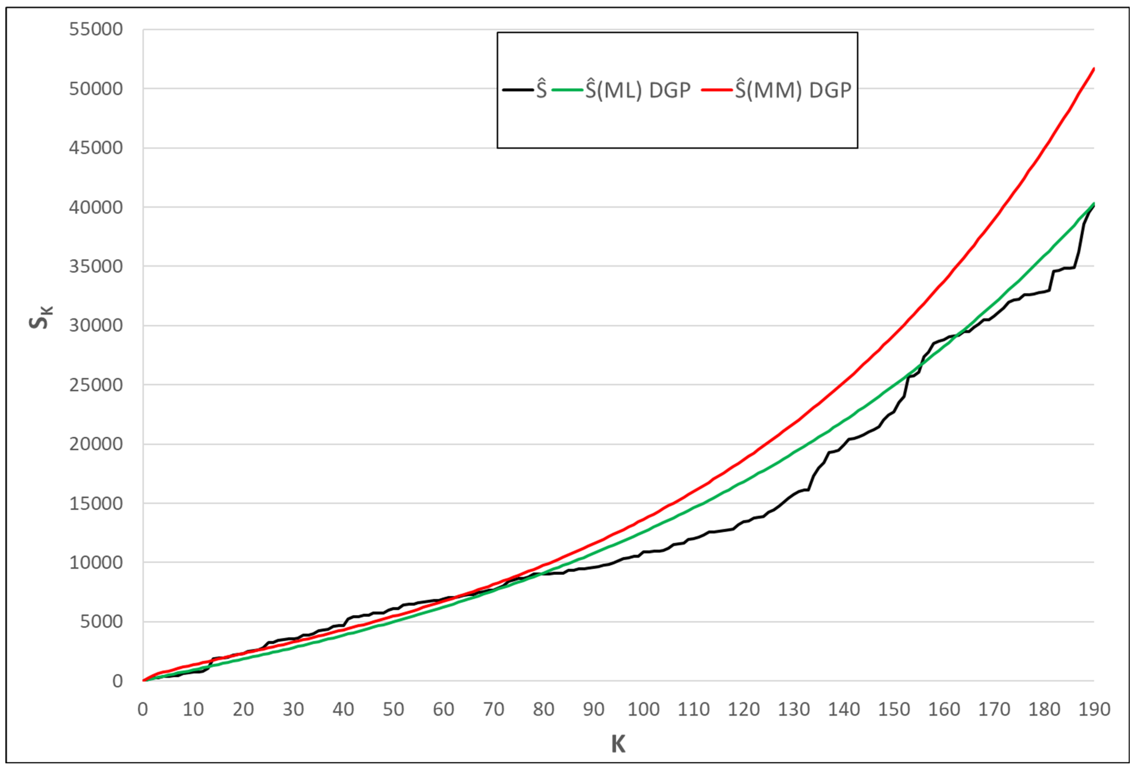
Figure 2.
The plots of and failure times for the data set 2.
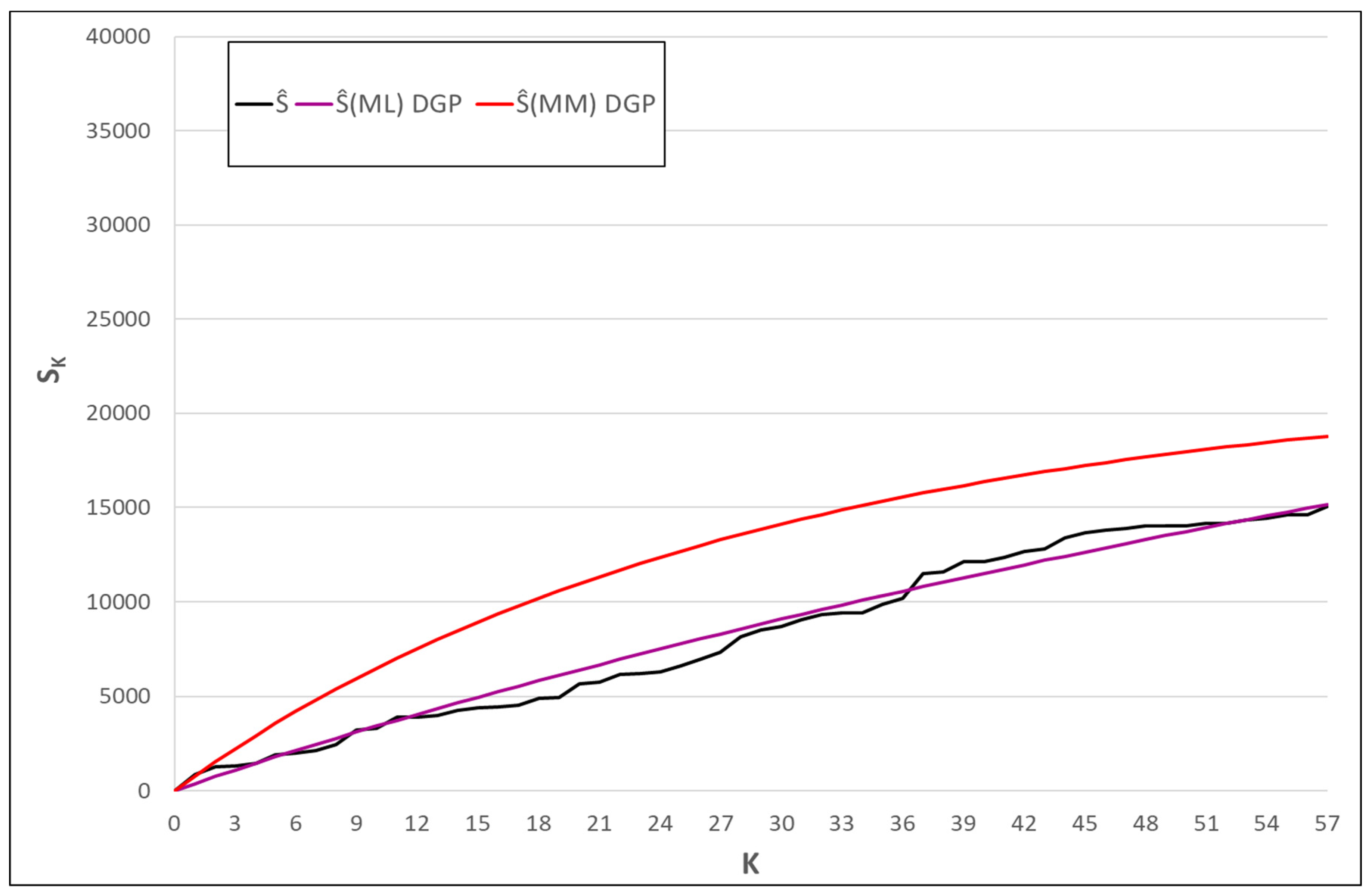
Table 1.
The biases and the MSEs for the ML estimators of the parameters , for values.
| Method | Mean | Bias | MSE | Mean | Bias | MSE | Mean | Bias | MSE | Mean | Bias | MSE | ||
| 0.95 | 30 | ML | 0.9453 | -0.0047 | 0.0004 | 2.0543 | 0.0543 | 0.0408 | 1.0882 | 0.0882 | 0.0811 | 1.9564 | 0.0436 | 0.3295 |
| 50 | ML | 0.9479 | -0.0021 | 0.0001 | 2.0263 | 0.0263 | 0.0172 | 1.0508 | 0.0508 | 0.0390 | 1.9597 | -0.0402 | 0.1965 | |
| 100 | ML | 0.9490 | -0.0009 | 0.00003 | 2.0119 | 0.0119 | 0.0069 | 1.0269 | 0.0269 | 0.0177 | 1.9806 | -0.0194 | 0.1050 | |
| 0.99 | 30 | ML | 0.9893 | -0.0007 | 0.0002 | 2.0456 | 0.0456 | 0.0358 | 1.0912 | 0.0912 | 0.0910 | 1.9374 | -0.0626 | 0.3348 |
| 50 | ML | 0.9891 | -0.0009 | 0.00005 | 2.0254 | 0.0254 | 0.0178 | 1.0435 | 0.0435 | 0.0388 | 1.9677 | -0.0328 | 0.1946 | |
| 100 | ML | 0.9897 | -0.0003 | 0.0000 | 2.0092 | 0.0092 | 0.0064 | 1.0291 | 0.0291 | 0.0178 | 1.9732 | 0.0268 | 0.1045 | |
| 1.01 | 30 | ML | 1.0089 | -0.0011 | 0.0001 | 2.0524 | 0.0524 | 0.0384 | 1.0904 | 0.0904 | 0.0866 | 1.9523 | -0.0477 | 0.3556 |
| 50 | ML | 1.0098 | -0.0002 | 0.00003 | 2.0250 | 0.0250 | 0.0176 | 1.0381 | 0.0381 | 0.0338 | 1.9821 | -0.0179 | 0.2039 | |
| 100 | ML | 1.0100 | 0.0000 | 0.0000 | 2.0109 | 0.0109 | 0.0059 | 1.0247 | 0.0247 | 0.0182 | 1.9675 | -0.0325 | 0.1067 | |
| 1.05 | 30 | ML | 1.0519 | 0.0019 | 0.0001 | 2.0546 | 0.0546 | 0.0427 | 1.0958 | 0.0958 | 0.0829 | 1.9335 | -0.0665 | 0.3369 |
| 50 | ML | 1.0510 | 0.0010 | 0.00003 | 2.0275 | 0.0275 | 0.0161 | 1.0434 | 0.0434 | 0.0356 | 1.9787 | -0.0213 | 0.1948 | |
| 100 | ML | 1.0505 | 0.0005 | 0.00001 | 2.0070 | 0.0070 | 0.0059 | 1.0335 | 0.0335 | 0.0199 | 1.9779 | -0.0220 | 0.1102 | |
Table 2.
The biases and the MSEs for the ML estimators of the parameters , for values.
| a | n | a | b | α | β | |||||||||
| Method | Mean | Bias | MSE | Mean | Bias | MSE | Mean | Bias | MSE | Mean. | Bias | MSE | ||
| 0.95 | 30 | ML | 0.9466 | -0.0034 | 0.0004 | -1.9493 | 0.0507 | 0.0416 | 1.0897 | 0.0897 | 0.0806 | 1.9494 | -0.0506 | 0.3582 |
| 50 | ML | 0.9477 | -0.0023 | 0.0001 | -1.9682 | 0.0318 | 0.0187 | 1.0467 | 0.0467 | 0.0377 | 1.9855 | -0.0145 | 0.1941 | |
| 100 | ML | 0.9488 | -0.0012 | 0.00003 | -1.9841 | 0.0159 | 0.0066 | 1.0302 | 0.0302 | 0.0184 | 1.9748 | -0.0252 | 0.1005 | |
| 0.99 | 30 | ML | 0.9876 | -0.0024 | 0.0002 | -1.9469 | 0.0531 | 0.0415 | 1.0932 | 0.0931 | 0.0791 | 1.9317 | -0.0683 | 0.3503 |
| 50 | ML | 0.9895 | -0.0005 | 0.00005 | -1.9755 | 0.0245 | 0.0177 | 1.0566 | 0.0566 | 0.0400 | 1.9628 | -0.0372 | 0.2049 | |
| 100 | ML | 0.9896 | -0.0004 | 0.0000 | -1.9875 | 0.0125 | 0.0064 | 1.0241 | 0.0241 | 0.0167 | 1.9766 | -0.0234 | 0.1015 | |
| 1.01 | 30 | ML | 1.0092 | -0.0008 | 0.0001 | -1.9423 | 0.0577 | 0.0399 | 1.0916 | 0.0916 | 0.0778 | 1.9299 | -0.0701 | 0.3468 |
| 50 | ML | 1.0097 | -0.00002 | 0.00003 | -1.9748 | 0.0252 | 0.0169 | 1.0602 | 0.0602 | 0.0412 | 1.9489 | -0.0510 | 0.2024 | |
| 100 | ML | 1.0100 | 0.0000 | 0.0000 | -1.9891 | 0.0109 | 0.0061 | 1.0312 | 0.0312 | 0.0199 | 1.9739 | -0.0261 | 0.1072 | |
| 1.05 | 30 | ML | 1.0520 | 0.0020 | 0.0001 | -1.9447 | 0.0553 | 0.0424 | 1.0830 | 0.0830 | 0.0786 | 1.9539 | -0.0461 | 0.3423 |
| 50 | ML | 1.0512 | 0.0012 | 0.00003 | -1.9720 | 0.0280 | 0.0158 | 1.0441 | 0.0441 | 0.0343 | 1.9759 | -0.0241 | 0.1963 | |
| 100 | ML | 1.0505 | 0.0005 | 0.00001 | -1.9918 | 0.0082 | 0.0060 | 1.0234 | 0.0234 | 0.0173 | 1.9855 | -0.0145 | 0.1068 | |
Table 3.
The biases and the MSEs for the ML estimators of the parameters , for values.
| Method | Mean | Bias | MSE | Mean | Bias | MSE | Mean | Bias | MSE | Mean | Bias | MSE | ||
| 0.95 | 30 | ML | 0.9464 | -0.0036 | 0.0002 | -1.9544 | 0.0456 | 0.0340 | 2.1875 | 0.1875 | 0.3753 | 0.9710 | -0.0290 | 0.0727 |
| 50 | ML | 0.9482 | -0.0018 | 0.00008 | -1.9775 | 0.0225 | 0.0151 | 2.1218 | 0.1218 | 0.2006 | 0.9778 | -0.0222 | 0.0470 | |
| 100 | ML | 0.9494 | -0.0006 | 0.00002 | -1.9934 | 0.0066 | 0.0054 | 2.0498 | 0.0498 | 0.0817 | 0.9929 | -0.0071 | 0.0217 | |
| 0.99 | 30 | ML | 0.9878 | -0.0022 | 0.0001 | -1.9502 | 0.0498 | 0.0355 | 2.2301 | 0.2301 | 0.4691 | 0.9625 | -0.0375 | 0.0728 |
| 50 | ML | 0.9890 | -0.0009 | 0.00003 | -1.9705 | 0.0294 | 0.0165 | 2.1177 | 0.1177 | 0.2005 | 0.9781 | -0.0219 | 0.0444 | |
| 100 | ML | 0.9897 | -0.0003 | 0.0000 | -1.9904 | 0.0096 | 0.0059 | 2.0589 | 0.0589 | 0.1177 | 0.9878 | -0.0122 | 0.0217 | |
| 1.01 | 30 | ML | 1.0088 | -0.0012 | 0.0001 | -1.9495 | 0.0505 | 0.0373 | 2.2403 | 0.2403 | 0.4407 | 0.9486 | -0.0514 | 0.0681 |
| 50 | ML | 1.0096 | -0.0004 | 0.00001 | -1.9720 | 0.0280 | 0.0167 | 2.1172 | 0.1172 | 0.1880 | 0.9807 | -0.0193 | 0.0475 | |
| 100 | ML | 1.0100 | 0.0000 | 0.0000 | -1.9878 | 0.0122 | 0.0059 | 2.0526 | 0.0526 | 0.0742 | 0.9902 | -0.0098 | 0.0212 | |
| 1.05 | 30 | ML | 1.0514 | 0.0014 | 0.00007 | -1.9497 | 0.0502 | 0.0344 | 2.1828 | 0.1828 | 0.3678 | 0.9771 | -0.0229 | 0.0811 |
| 50 | ML | 1.0511 | 0.0011 | 0.00002 | -1.9732 | 0.0268 | 0.0148 | 2.1393 | 0.1393 | 0.1947 | 0.9695 | -0.0305 | 0.0411 | |
| 100 | ML | 1.0507 | 0.0007 | 0.00001 | -1.9884 | 0.0116 | 0.0055 | 2.0508 | 0.0508 | 0.0818 | 0.9930 | -0.0070 | 0.0237 | |
Table 4.
The biases and the MSEs for the ML estimators of the parameters , for values.
| Method | Mean | Bias | MSE | Mean | Bias | MSE | Mean | Bias | MSE | Mean | Bias | MSE | ||
| 0.95 | 30 | ML | 0.9463 | -0.0037 | 0.0003 | 2.0438 | 0.0438 | 0.0372 | 2.2241 | 0.2241 | 0.4240 | 0.9625 | -0.0375 | 0.0728 |
| 50 | ML | 0.9478 | -0.0021 | 0.0001 | 2.0300 | 0.0300 | 0.0166 | 2.0883 | 0.0883 | 0.1559 | 0.9896 | -0.0104 | 0.0420 | |
| 100 | ML | 0.9491 | -0.0008 | 0.00002 | 2.0121 | 0.0121 | 0.0062 | 2.0501 | 0.0501 | 0.0763 | 0.9896 | -0.0037 | 0.0221 | |
| 0.99 | 30 | ML | 0.9880 | -0.0019 | 0.0001 | 2.0396 | 0.0396 | 0.0340 | 2.1938 | 0.1938 | 0.3321 | 0.9612 | -0.0387 | 0.0701 |
| 50 | ML | 0.9891 | -0.0008 | 0.00003 | 2.0251 | 0.0251 | 0.0160 | 2.1193 | 0.1193 | 0.1822 | 0.9746 | -0.0254 | 0.0417 | |
| 100 | ML | 0.9897 | -0.0003 | 0.0060 | 2.0075 | 0.0075 | 0.0060 | 2.0436 | 0.0436 | 0.0766 | 0.9992 | -0.0008 | 0.0222 | |
| 1.01 | 30 | ML | 1.0089 | -0.0011 | 0.0001 | 2.0549 | 0.0549 | 0.0363 | 2.2212 | 0.2212 | 0.4298 | 0.9662 | -0.0337 | 0.0745 |
| 50 | ML | 1.0095 | -0.0005 | 0.00001 | 2.0299 | 0.0299 | 0.0152 | 2.1384 | 0.1384 | 0.1837 | 0.9711 | -0.0289 | 0.0436 | |
| 100 | ML | 1.0100 | 0.0000 | 0.0000 | 2.0077 | 0.0077 | 0.0053 | 2.0680 | 0.0680 | 0.0790 | 0.9864 | -0.0136 | 0.0212 | |
| 1.05 | 30 | ML | 1.0515 | 0.0015 | 0.0000 | 2.0564 | 0.0564 | 0.0339 | 2.1952 | 0.1952 | 0.3772 | 0.9706 | -0.0293 | 0.0736 |
| 50 | ML | 1.0511 | 0.0011 | 0.0000 | 2.0268 | 0.0268 | 0.0149 | 2.0947 | 0.0947 | 0.1765 | 0.9919 | -0.0081 | 0.0464 | |
| 100 | ML | 1.0506 | 0.0006 | 0.0000 | 2.0136 | 0.0136 | 0.0049 | 2.0499 | 0.0499 | 0.0744 | 0.9873 | -0.0126 | 0.0215 | |
Table 13.
The number, reference, and sample size of the data set 2.
| Data set no | References | |
| 1 | Maguire (1952) | 190 |
Table 14.
The KS test statistic value and p-value for dataset set1.
| KS test statistic | p value |
| 0.0526 | 0.8931 |
Table 15.
The results for the investigated methods for dataset set 1 in DGP.
| MSE | MPE | |||||||
| ML | 0.988 | 0.095 | 0.737 | 152.41 | 56634.3 | 0.46042 | 112.403 | 17131.470 |
| MM | 0.977 | 0.351 | - | - | 85329.2 | 1.47735 | 285.635 | 279715.86 |
Table 16.
The number, reference, and sample size of the data set 2.
| Data set no | References | Sample size |
| 2 | Stanwick Corporation (1965). | 57 |
Table 17.
The KS test statistic value and p-value for dataset set2.
| KS test statistic | p value |
| 0.0737 | 0.8941 |
Table 18.
The results for the investigated methods for dataset 2.
| MSE | MPE | |||||||
| ML | 1.0089 | 0.0283 | 0.9187 | 419.222 | 66073.03 | 0.5495 | 385.1392 | 161458.84 |
| MM | 1.0349 | 0.0155 | - | - | 92589.38 | 1.2610 | 788.466 | 836326.4 |
Disclaimer/Publisher’s Note: The statements, opinions and data contained in all publications are solely those of the individual author(s) and contributor(s) and not of MDPI and/or the editor(s). MDPI and/or the editor(s) disclaim responsibility for any injury to people or property resulting from any ideas, methods, instructions or products referred to in the content. |
© 2025 by the authors. Licensee MDPI, Basel, Switzerland. This article is an open access article distributed under the terms and conditions of the Creative Commons Attribution (CC BY) license (http://creativecommons.org/licenses/by/4.0/).
Copyright: This open access article is published under a Creative Commons CC BY 4.0 license, which permit the free download, distribution, and reuse, provided that the author and preprint are cited in any reuse.