
Submitted:
19 August 2025
Posted:
20 August 2025
You are already at the latest version
Abstract
Due to the globalization of supply chains and the resulting increase in the quantity and diversity of suppliers, the segmentation of suppliers has become fundamental to improving relationship management and supplier performance. Moreover, given the need to incorporate the concept of sustainability into supply chain management, criteria based on economic, environmental and social performance have been adopted in evaluating suppliers. However, there are few studies that present sustainable supplier segmentation models in the literature, and none of them makes it possible to predict individual supplier performance for each TBL dimension in a non-compensatory manner. Moreover, none of them permits the use of historical performance data to adapt the model to the usage environment. Given this, the objective of this study is to propose a decision-making model for sustainable supplier segmentation using an adaptive network-based fuzzy inference system (ANFIS). Our approach combines three ANFIS computational models in a tridimensional quadratic matrix, based on diverse criteria associated with the dimensions of the triple bottom line (TBL). A pilot application of this model in a sugarcane mill was performed. We implemented 108 candidate topologies by means of the Neuro-Fuzzy Designer of the MATLAB® software. The cross-validation method was applied to select the best topologies. The accuracy of the selected topologies was confirmed using statistical tests. The proposed model can be adopted for supplier segmentation processes in companies that wish to monitor and/or improve the sustainability performance of their suppliers. This study may also be useful to researchers in developing computational solutions for segmenting suppliers, mainly in terms of ANFIS modeling and providing appropriate topological parameters to obtain accurate results.
Keywords:
sustainable supplier segmentation
; ANFIS
; supplier categorization
; sustainable supply chain management
1. Introduction
Over the past few decades, more rigid environmental legislation and stakeholder pressure for greater profitability have made companies promote improvements in the sustainability of their operations (Finger and Lima, 2022). According to Bai et al. (2021, p.1), the implementation of sustainability “requires organizations to extend their focus beyond the traditional economic objectives to embrace a triple-bottom-line (TBL) approach that requires them to simultaneously meet or make trade-offs between economic, environmental and social goals”. These authors also point out that it is quite difficult to achieve sustainability in a company’s operations without the support of its suppliers. Within this context, supplier relationship management has become essential to optimizing the supplier base and making the performance of the supply chain more sustainable (Shiralkar et al., 2022; Lima et al., 2023).
With the advent of global supply chains, the quantity and diversity of suppliers available in the market has increased drastically, which has made managing supplier relationships more complex (Zimmer et al., 2016; Resende et al., 2023). Given this, the segmentation of suppliers presents itself as an effective way to manage the supplier base, because by grouping suppliers that have characteristics in common, it limits the number of relationship strategies necessary to manage the supplier base and promote more effective management (Bai et al., 2017). Supplier segmentation can help managers allocate specific resources to certain relationships to create development strategies that are appropriate for the supplier’s profile (Borges et al., 2022).
In the literature there are various studies which propose the use of quantitative models to support the supplier segmentation process (Shiralkar et al., 2022). In recent years, this subject has received more interest from researchers given the capacity of these models to support decision-making in an automated manner (Resende et al., 2023). In general, classifying suppliers into groups is based on a group of criteria associated with the dimensions of the supplier’s performance (Bai et al., 2017; Rezaei and Lajimi, 2019). Even though there are dozens of decision-making models to support supplier segmentation, most of them classify suppliers only based on economic aspects (Borges et al., 2022).
As shown in Table 1, based on the studies in a systematic review of this subject (Day et al., 2010; Borges and Lima, 2020; Shiralkar et al., 2022) and bibliographic research realized for this study, we have found just nine studies which propose quantitative models to support sustainable supplier segmentation (Torres-Ruiz and Ravindran, 2018; Rius-Sorolla et al., 2020; Borges et al., 2022, Coşkun et al., 2022; Mavi et al., 2023; Paybarjay et al., 2023; Rahiminia et al., 2023; Taghipour et al., 2023; Li et al., 2024). In other words, just nine models took into consideration economic, environmental and social criteria in the supplier segmentation process.
The sustainable supplier segmentation models proposed by Torres-Ruiz and Ravindran (2018), Rius-Sorolla et al. (2020), Borges et al. (2022), Mavi et al. (2023), Rahiminia et al. (2023), and Taghipour et al. (2023) are compensatory, which means poor performance in some criteria of a given dimension can be compensated for by good performance in criteria in other dimensions. Within the context of sustainable supply chains, economic aspects should not be allowed to compensate for environmental and social aspects (Schramm et al., 2020). Only the models proposed by Coşkun et al. (2022), Paybarjay et al. (2023), and Li et al. (2024) allow for the segmentation of suppliers based on TBL dimensions without compensation among the criteria associated with these dimensions.
Moreover, despite the diversity of the techniques explored for sustainable supplier segmentation, none of the models in the literature have a supervised learning procedure based on historical performance data (Borges and Lima, 2020; Shiralkar et al., 2022). This constraint complicates the utilization of data from periodic supplier evaluations to adjust cause-and-effect relationships between input variables and output variables in the model. Even though all of the existing models for sustainable supplier segmentation are based on Multi-criteria Decision Making (MCDM) methods, they cannot be tuned based on historical data. In addition, since MCDM methods usually provide a global rating for each alternative based on a weighted combination of model inputs, MCDM methods are not capable of mapping functions which indicate the cause-and-effect relationships between the input and output variables. Depending on which indicators are adopted, their relationships may not be linear (for example, x=y/z or x=z.y2), which also makes MCDM methods inappropriate in these cases. The proposal of a new decision-making model for sustainable supplier segmentation using adaptive network-based fuzzy inference systems (ANFISs) can get around these limitations.
ANFISs are hybrid systems which combine artificial neural networks and fuzzy inference. They are able to adapt to the usage environment based on supervised learning and are also appropriate for decision making under conditions of uncertainty (Lima and Carpinetti, 2020). In this way, after training the ANFIS models using supplier performance data, these models can predict global performance values for the suppliers for each TBL dimension (Bamakan et al., 2021).
In this context, the objective of this article is to propose a decision-making model for sustainable supplier segmentation based on ANFISs. A pilot application of this model has been performed to test its use and select the best ANFIS topologies for each TBL dimension. Statistical tests were performed to analyze the accuracy of the implemented computational models and validate the proposal. The rest of the article is organized in the following manner. Section 1 will present the theoretical references concerning sustainable supplier segmentation and ANFIS systems. Section 2 will detail the proposed model, while Section 3 will present the results of its application. Section 4 will discuss the results of the statistical tests used to validate the model. Finally, conclusions and the limitations of this study are presented.
2. Theoretical Framework
2.1. Sustainable Supplier Segmentation
Shiralkar et al. (2022, p.1) claim that “global firms need to expand their supplier base in other parts of the world instead of relying only on their supplier base from one country to manage global disruptions due to pandemics or other environmental factors more effectively.” In this context, when formulating supplier relationship strategies to deal with a large number of global suppliers, there is a need to establish a manageable number of supplier categories based on specific features or dimensions (Rezaei and Lajimi, 2019; Shiralkar et al., 2022).
Day et al. (2010, p.626) conceptualized supplier segmentation as “a process that involves the division of suppliers into distinct groups, with different needs, characteristics, or behavior, requiring different types of relationship structures between companies in order to obtain exchange value”. The inclusion of environmental and social criteria makes the supplier segmentation process more effective (Borges et al., 2022; Shiralkar et al., 2022), given that the economic, social and environmental commitment to stakeholders has required the adoption of practices to improve the sustainable performance of suppliers (Finger and Lima, 2022). Social and environmental performance improvements are beneficial to organizations because they fulfill the needs of the stakeholders and indirectly carry out economic improvements (Rius-Sorolla et al., 2020). Thus, supplier segmentation based on the TBL criteria has become a crucial practice that enables companies to improve their supply chain sustainability (Shiralkar et al., 2022).
Table 2 presents some criteria suggested by the literature to evaluate supplier performance in accordance with the three dimensions of TBL. The use of economic criteria is essential to promote economic growth, efficient logistics, and a good level of quality. Environmental criteria aim to ensure the protection of the natural environment and reductions in the use of resources, while social criteria are related to the creation of productive employment and equality (Rius-Sorolla et al., 2020).
To classify suppliers in terms of each performance dimension in the supplier segmentation process, a suitable decision-making method needs to be applied (Rezaei and Ortt, 2013). The literature presents several studies that propose supplier segmentation models based on decision-making methods to categorize suppliers into segmentation matrices. Given the importance of this topic, several literature review studies have been conducted (Day et al., 2010; Borges and Lima, 2020; Shiralkar et al., 2022).
Day et al. (2010) presented a systematic review involving dozens of theoretical models to support the supplier segmentation process. Based on their analysis of the structural elements of these models, Day et al. (2010) developed a detailed taxonomic classification of previous supplier segmentation research. Borges and Lima (2020) reviewed 26 studies that propose decision-making models for supplier segmentation. Shiralkar et al. (2022) presented a summary of the multicriteria decision-making (MCDM) methods used in supplier segmentation and discussed their limitations.
Table 3 lists some of the studies that propose decision-making models for supplier segmentation. This table only presents studies published since 2013 with the goal of updating the state of the art concerning this subject, and it includes some models which have not appeared in previous systematic reviews of the literature proposed by Day et al. (2010), Borges and Lima (2020), and Shiralkar et al. (2022). These studies were collected based on the Science Direct, Springer, Scopus, Emerald Insight, IEEE Xplore®, Taylor & Francis, and Wiley databases, in accordance with the procedures presented by Borges and Lima (2020). In addition to indicating the decision-making techniques used in each model, Table 3 describes the performance dimensions considered in the supplier segmentation matrices. This table also indicates the type of supply chain management strategy considered in each study, which is directly related to the segmentation dimensions and the supplier evaluation criteria adopted in each case.
In Table 3, we may note that most of these studies applied the AHP method (Rezaei and Ortt, 2013b; Santos et al., 2017; Segura and Maroto, 2017; Torres-Ruiz and Ravindran, 2018; Bianchini et al., 2019). The methods based on Fuzzy Set Theory have been also prominent, such as the Fuzzy C-Means method (Haghighi et al., 2014; Akman, 2015; Jharkharia and Das, 2019; Matshabaphala and Grobler, 2021), the Fuzzy-TOPSIS method (Bai et al., 2017; Medeiros and Ferreira, 2018), and the Fuzzy-AHP method (Haghighi, Morad and Salahi, 2014; Lo and Sudjatmika, 2016, Mavi et al., 2023).
In terms of the performance dimensions that make up the axes of the supplier segmentation matrices, the most used were supplier capabilities and supplier willingness. As shown in Table 3, most of the studies have considered a traditional supply chain management strategy, which is more focused on economic performance. We found just eight models oriented towards sustainable supplier segmentation: Torres-Ruiz and Ravindran (2018), Rius-Sorolla et al. (2020), Borges et al. (2022), Coşkun et al. (2022), Mavi et al. (2023), Paybarjay et al. (2023), Rahiminia et al. (2023), and Taghipour et al. (2023).
In Torres-Ruiz and Ravindran (2018), the authors use the AHP (Analytic Hierarchy Process) method to segment suppliers based on measures of sustainability risk. Even though the AHP method is the most utilized in the supplier segmentation literature (Borges and Lima, 2020), it has a few disadvantages. Its main limitation is the number of criteria and alternatives that can be adopted, because the evaluations are realized by specialists through paired comparisons (Borges et al., 2022). In addition, when new suppliers are added to the database, inversions may occur in the results.
Even though the decision-making model proposed by Rius-Sorolla et al. (2020) considers three dimensions of criteria for sustainability, this model does not use a specific decision-making technique. This approach just weighs and aggregates supplier evaluations using mathematical equations based on crisp numbers. Thus, the proposed model is not appropriate for dealing with qualitative criteria, nor can it model and process the subjective judgments of specialists. Thus, similarly to the model proposed by Rahiminia et al. (2023), the approach developed by Rius-Sorolla et al. (2020) is inappropriate for handling decision making under uncertainty.
The model proposed by Borges et al. (2022) meanwhile, uses the Hesitant Fuzzy Linguistic TOPSIS method for segmenting suppliers in a matrix subdivided into two dimensions: “capacities” and “willingness to collaborate”. Coşkun et al. (2022) present an interesting model for segmenting sustainable suppliers. Their model is based on ANP, PROMETHEE, and cluster analysis. Meanwhile, the model developed by Paybarjay et al. (2023) combines BWM and Grey Simple Additive weighting to support supplier development through sustainable supplier segmentation.
Mavi et al. (2023) utilized Fuzzy-AHP and Fuzzy equivalence relation to segment suppliers based on economic, environmental, social, and risk criteria. Rahiminia et al. (2023) integrated BWM and K-means to cluster sustainable suppliers according to profit impact and supply risks. Taghipour et al. (2023) introduced a segmentation model based on BWM and PROMETHEE to categorize suppliers using a two-dimensional matrix. With the exception of the studies by Coşkun et al. (2022) and Paybarjay et al. (2023), all sustainable supplier segmentation models in the literature adopted a compensatory approach. This means that high performance in one dimension partially offsets low performance in another dimension. However, the use of compensatory approaches does not allow for the identification of suppliers that exhibit low performance in specific dimensions, thus hindering the attainment of a balanced performance level across all three dimensions of the TBL. Additionally, compensatory models lack the capacity to identify the need for direct actions to improve economic, environmental, and/or social aspects.
Another limitation of previous supplier segmentation models is their difficulty in adapting to the specific usage environment, as well as their challenge in modeling non-linear relationships among performance measures. Despite the variety of techniques displayed in Table 3, none of them is able to tune the model’s parameters to the usage environment based on historical performance data. Furthermore, the only ones that are based on decision-making rules are those based on fuzzy inference systems (Osiro et al., 2014; Aloini et al., 2019; Rajesh and Raju, 2021). Nevertheless, the manual parameterization of dozens or hundreds of rules required by these inference systems makes the modeling phase exceedingly time-consuming for decision-makers, and furthermore, may lead to inconsistent results due to errors in rule settings. Thus, since the previous models do not use any supervised learning algorithm, they are not able to computationally adjust cause and effect relationships between the input and output variables. The development of ANFIS models to support the supplier segmentation process can overcome these limitations.
2.2. Adaptive Neuro-Fuzzy Inference Systems
In the literature there are various types of techniques that combine fuzzy logic with artificial neural networks, and they are generally known as neuro-fuzzy systems (Lima and Carpinetti, 2020). The most popular of these was proposed by Jang (1993) and it is called an Adaptive Neuro-Fuzzy Inference System or Adaptive-Network-Based Fuzzy Inference System (ANFIS). As discussed in Section 1.1, the application of fuzzy inference systems requires a considerable effort to define inference rules and membership functions (Shiralkar et al., 2022). Neural networks, on the other hand, when they are used in an isolated manner, do not promote transparency in their calculations and are not appropriate for making decisions under conditions of uncertainty. These limitations can be overcome by a combination of these two techniques which generates a model with superior predictive capacity and greater transparency in terms of its results (Özkana and Inal, 2014; Bamakan et al., 2021).
Figure 1 presents the topology of the ANFIS model with three input variables and one output variable. This system possesses five layers and within each one there are nodes that perform the same types of functions. The fixed nodes are represented by circles, while squares indicate the adaptive nodes. The adaptive nodes are adjusted during system training through modifiable parameters. The functioning of each layer is described below (Lima and Carpinetti, 2020):
- a)
- Layer 1: In this layer the input values (x and y) in crisp format are converted into fuzzy sets equivalents. Their function can be given as:
- b)
- Layer 2: This layer combines all of the nodes of the previous layer with the objective of establishing the logical relationships among the activated membership functions. This layer represents the antecedent part of the decision-making rules, which realizes operations of the type “AND” or “OR”. The equation that represents the realized operation for this combination layer is given by:
- c)
- Layer 3: This layer normalizes the weights of the activated rules. Equation 3 describes the procedure.
- d)
- Layer 4: This is the layer of the adaptive nodes which represents the rule consequents. These consequents generate outputs for each activated rule according to Equation 4. The consequent value can be produced by a linear function or a constant function. The output value of this layer is calculated by the simple product of the consequent of each rule () and the weight of the rule activated in the third layer;
- e)
- Layer 5: This layer is composed of a fixed node which calculates a weighted sum of the outputs of the previous layer, as represented by Equation 5.
To conduct the learning process for an ANFIS, one needs to have sample values for the input variables and the output variable. These samples should be divided into two groups: 60 to 90% of the samples for the training set, and 10 to 40% for the validation set. The first set should be used to adjust the adaptive parameters. The second set should be applied to verify the model’s accuracy (Özkan and Inal, 2014; Bamakan et al., 2021).
One of the supervised learning algorithms that is most often used to train ANFIS models is the hybrid algorithm proposed by Jang (1993). This algorithm applies the least squares method to adjust adaptive parameters for the inputs, and the gradient descent method to adjust the consequents of the rules in order to minimize the errors between the values produced by the model and the output value of each training sample. The number of times that the training samples are processed by the model is called the epoch number, which serves as a stop criterion (Lima and Carpinetti, 2020). After the training has been completed, the validation of the model can be performed based on the MSE (mean square error) obtained using the validation set.
The type of the membership function, the number of membership functions, and the types of consequent and logical operators are the parameters which directly affect the accuracy of ANFIS models. This is why it is necessary to perform various computational tests to select the best topology for each model. The cross-validation technique can be adopted to support the choice of the best topologies. This technique is based on the realization of several tests by varying the values of the model’s topological parameters (Lima and Carpinetti, 2020).
3. The Proposed Model for Sustainable Supplier Segmentation
Our theoretical model designed to support sustainable supplier segmentation is presented in Figure 2. This model is divided into three steps and was developed based on Silva et al. (2016), Lima and Carpinetti (2020), Lajimi (2021), and Pedroso et al. (2021). It involves the use of three ANFIS computational models, one for each TBL dimension. Besides permitting the grouping of suppliers based on similar performance levels, the proposed model offers a base for the elaboration of action plans that seek to develop suppliers in economic, environmental, and social terms.
Stage 1 begins with the assembling of a decision-making team (Step 1.1). This team should be made up of professionals from the sales, quality management, socio-environmental management, and/or supplier development areas, as well as other employees linked to supply chain management. In Step 1.2, the team will select the most important criteria to be analyzed for each TBL dimension, and the selected criteria should be aligned with the company’s performance targets. Some examples of possible criteria for each dimension are presented in Table 2.
Step 1.3 involves the definition of the suppliers which will be evaluated by the buying company. The focus of this evaluation is the suppliers which are qualified and have already been hired by the buying company. In Step 1.4, a score is assigned individually for the performance of each supplier in relation to each criterion chosen in Step 1.2. These scores can be defined based on historical data from the buying company through performance indicators, ERP (Enterprise Resource Planning) systems, or BI (Business Intelligence) systems, among other management support systems. In the absence of historical data, or when it is insufficient, it is possible to form a committee of decision makers (DMs) in supply chain related areas to collect the opinions of these specialists in judging these suppliers in terms of each criterion.
In Step 1.5, the cross-validation technique must be applied to build and tune the ANFIS models. By using this method, various topologies of the ANFIS models can be tested to select those capable of achieving the greatest accuracy in their results. Figure 3 presents the steps of applying the proposed cross-validation technique designed specifically for ANFIS systems. In the first step, the samples should be subdivided into two groups: the training set and the validation set (i). Then, the topology candidates should be defined by varying the values of the internal parameters of each ANFIS model (ii). The values for each parameter to be tested should be defined based on the literature or through empirical computational tests.
After defining the candidate topologies, the supervised learning process should be determined using a suitable computation tool (iii). In this study, we used the Neuro-Fuzzy Designer of the MATLAB MathWorks® software for the training and validation of the ANFIS topologies. The set of training samples should be applied to tune the internal parameters of each ANFIS model. After completing the training, the validation of each topology should be made based on the MSE achieved by each of them. The MSE is calculated based on a comparison between the predicted output value and the expected output value for each validation sample. If one or more of the topologies attains an acceptable MSE level, the topology with the lower MSE should be selected (iv). Otherwise, we suggest changing the number of membership functions, increasing the number of samples, and/or changing the quantity of epochs (v).
Stage 2 focuses on applying the ANFIS models to the supplier segmentation process. Step 2.1 consists of defining the suppliers to be segmented based on the TBL dimensions, while Step 2.2 focuses on obtaining the scores of these suppliers for each criterion. Since collecting data from all of the suppliers can be difficult and time consuming, it is recommended that it only include suppliers that are important to the company, such as the suppliers of strategic, leverage or bottleneck items. In Step 2.3, the supplier scores for each criterion should be input into the ANFIS system which has been trained in the previous stage. Then, each ANFIS model will estimate the global performance of each supplier in a specific dimension. While the ANFIS 1 model will calculate the overall performance values regarding the environmental dimension, the ANFIS 2 and 3 models will estimate the overall performance regarding the social and economic dimensions respectively.
In Stage 3 of the proposed model, each supplier should be classified in one of eight possible groups defined in Figure 4. This classification helps buyers define appropriate actions to manage their supplier base and improve the performance of the suppliers. Each dimension of the segmentation matrix represents a TBL dimension. Each group is represented as Gi(f(Y1), f(Y2), f(Y3)), with (i = 0, 1, …, 8). The values of f(Ym) (m = 1, …, 3) indicate the supplier classification results for each dimension. If f(Ym) ≥ tm, then f(Ym) = “High (H)”. Otherwise, f(Ym) = “Low (L)”. The values of tm should be defined by the team of DMs according to the importance of these suppliers to the purchasing company.
In the matrix shown in Figure 4, suppliers which have presented similar performance for the three TBL dimensions must be classified in the same group. The features of the suppliers classified in each one of the groups shown in Figure 4 are described as follows (Lajimi et al., 2021):
- a)
- G1 (L, L, L) – This group consists of the suppliers which have presented the worst performance evaluations, or those which presented poor economic, environmental, and social performance. The suppliers in this group should be substituted if possible according to Lajimi et al. (2021). Otherwise, supplier development programs should be implemented to achieve improved supplier performance in the three dimensions of the TBL;
- b)
- G2 (H, L, L) – This group consists of suppliers which have achieved good environmental performance and poor economic and social performance. The suppliers in this segment generally focus on the efficient use of natural resources and the control and prevention of pollution;
- c)
- G3 (L, L, H) – This group consists of suppliers with good economic performance and poor social and environmental performance. They operate their supply chains with a focus on profits and are not concerned with environmental and social issues;
- d)
- G4 (H, L, H) – This group consists of suppliers with satisfactory economic and environmental performance, but poor social performance. They generally reduce costs through their efficient use of energy and natural resources;
- e)
- G5 (L, H, L) – This group consists of suppliers with good social performance and poor economic and environmental performance. They are focused on social justice. They emphasize diversity in their labor, human rights, a reduction in inequality, and the quality of life of their employees;
- f)
- G6 (H, H, L) – This groups consists of suppliers with poor economic performance and good social and environmental performance. They emphasize using a just portion of natural resources in both the domestic and international spheres;
- g)
- G7 (L, H, H) – This group consists of suppliers with good social and economic performance and poor environmental performance. These suppliers seek to reduce costs considering the social needs of society. They have ethical standards and ensure just business practices that protect the human rights of their employees;
- h)
- G8 (H, G, G) – This group consists of sustainable suppliers which have good social, economic, and environmental performance. They focus on improving their products and the quality of life of people, prioritizing environmental activities, and maximizing renewable natural resources at the least possible cost.
The results of supplier segmentation using the proposed approach make it possible for managers to formulate action plans to move their suppliers toward Group 8 (sustainable suppliers). These plans can be based on specific strategies for each supplier group to improve supplier management effectiveness and fill in the identified performance gaps. Table 4 presents some suggested supplier development strategies, separated by TBL dimension.
4. Application Case Study
4.1. Presentation of the Company
The pilot application of the proposed model was performed in a sugarcane mill. This mill is one of a group of companies located in various states in Brazil. The company in question is seeking to continually improve the sustainability of its operations through actions that involve stakeholders such as suppliers, commercial partners, and the local community. The company has an integrated management system which encompasses quality and environmental management and worker safety. This system contributes to the improvement of internal operations, facilitates supplier integration, and the obtaining of information for decision makers.
The company has more than 1,400 registered suppliers, with most of them being small sugarcane producers located near the mills. It also has international suppliers, which mainly supply fertilizers. The company seeks to work with suppliers which are aligned with its values of environmental preservation, continual improvement, and social responsibility. It also seeks to strengthen its relationships with its suppliers and develop partnerships with them. The group of mills coordinates various supplier development programs, which range from training and periodic meetings to exchange knowledge to the implementation of continual improvement programs, cost reductions, and improved worker safety.
The firm has an environmental risk prevention program which seeks to make the work environment safer while contributing to preserving the safety of its employees and its suppliers. This program includes training such as preventing and controlling the risk of fires in the sugarcane fields. The social programs include gathering and distributing clothes and blankets to people in need. There are also programs that promote education and culture in the communities where the sugarcane mills are located.
To improve the sustainability of its operations and meet the requirements of the international market, the company has obtained a certification from the Environmental Protection Agency and also has a RenovaBio seal, whose objective is to expand the sustainable production of biofuels in Brazil and reduce greenhouse gas emissions. All of the energy produced by this company comes from sugarcane biomass, which is a source of clean and renewable energy. The company produces all of the energy consumed by its operations, and the excess energy is commercialized. There are solid waste management programs that ensure the reincorporation of some production wastes (mainly sugarcane bagasse) or their appropriate disposal.
4.2. Application of the Proposed Model
4.2.1. Stage 1: Definition, Training, and Validation of the ANFIS Models
A group of DMs was defined as consisting of four company employees who directly participate in supply management: one from the supply department, another from the quality department, an environmental manager, and a work safety engineer. The experience of these DMs ranged from 4 to 9 years in the company. Three meetings were held with the DMs. The first presented the model and defined the criteria. The second defined the suppliers and the collection of their supplier evaluations. The third meeting analyzed the results provided by the model.
Initially, one of the authors of this study explained each step of the proposed model to the DMs as well as their roles. Then, the DMs initiated a discussion to define the supplier segmentation criteria to be adopted in this pilot application. This discussion was supported by the criteria displayed in Table 1 and the internal supplier evaluation forms. Based on this discussion, the DMs opted to: select the criteria that were already used by the company in the supplier evaluation process, which facilitated the obtaining of data to train the model; and adopt three or four criteria for each TBL dimension in order to prioritize the selection of crucial criteria for each dimension.
In total, the DMs selected 12 criteria to evaluate supplier performance. For the environmental dimension (ANFIS 1), they chose the criteria pollution control (C1), environmental management system (C2), resource consumption (C3), and recycling program (C4). For the social dimension (ANFIS 2), they selected employment practices (C5), health and safety (C6), and local community influence (C7). Finally, for the economic dimension (ANFIS 3), the criteria cost (C8), quality (C9), delivery time (C10), flexibility (C11) and technology capability (C12) have been chosen. The DMs have assigned all of these criteria equal weight within each dimension. It should be emphasized that these criteria have been selected just for this application, and future applications can use other criteria which are in line with the reality of each particular company.
For this study, we collected samples containing 200 supplier evaluations. The values of the supplier evaluations for the selected criteria (input variables) were obtained from the performance history of the suppliers. These values were extracted by using the supplier evaluation tool within the company's ERP system. The scales utilized varied with the criteria, so each criterion has a specifically defined domain. For the criteria C1, C3, C4, and C9, the values varied between 0 to 100, using a percentage score. For the criteria C2, C5, C6, C7, C8, C10, C11 and C12, the scores ranged from 0 to 10. The output variables (the global performance of the supplier for each TBL dimension) were calculated using the TOPSIS technique based on the collected input data. Table 5 illustrates the obtained supplier score samples for the supervised learning processes for the ANFIS 1 model.
To perform the supervised learning process for each of the ANFIS models through the use of cross-validation, the samples were separated into two sets. The first set, corresponding to 70% of the samples, was used in the training process. The second set, with 30% of the samples, was reserved for the validation process. Based on Lima and Carpinetti (2020), the number of training epochs was defined to be 30.
The tested topologies for the ANFIS models are presented in Table 6. The topological parameters were defined based on several previous studies which have applied ANFIS to supply chain management problems. For the partitioning of the input variables, we tested triangular, trapezoidal and Gaussian functions (Mavi et al., 2017; Bamakan et al., 2021). For the consequent type of the inference rules, we tested linear functions and constant values (Jang 1993; Lima, Carpinetti, 2020). Regarding the number of input partitions, we tested 3, 4, and 5 partitions (Akkoç, 2012; Mavi et al., 2017). Finally, in terms of fuzzy operators for the connectives of the inference rules, we tested the minimum and algebraic product operators (Jang, 1993; Lima, Carpinetti, 2020). With these procedures, we arrived at a total of 108 topologies tested, representing 36 for each ANFIS model.
Table 7, Table 8 and Table 9 present the results achieved during the computation implementation of the candidate topologies for models ANFIS 1, 2 and 3 respectively. During the training and validation of the candidate topologies, we calculated the MSE values. Based on Fan et al. (2013), the maximum MSE deemed acceptable for a topology was defined as Ɛ = 5 x 10⁻³. During the learning process for the topological candidates, we verified that the MSE had not stabilized by epoch 30. Thus, we opted to increase the number of training epochs gradually with this value being altered to 500, as proposed by Akkoç (2012). The candidate topologies which achieved the most accuracy, or in other words, the ones which achieved the lowest MSE values within the expected values and the predicted values in the validation step for each ANFIS model have been highlighted in bold.
The results of the computational implementation of the ANFIS models show that the Gaussian functions had the best performance for the three ANFIS models. Topologies of three input partitions produced the best result for two ANFIS models, and the use of four input partitions produced the best results for the other models. Topologies based on the crisp consequents and the product operator were the ones that achieved the lowest MSEs. Furthermore, the results demonstrate that the lower the number of input variables is, the greater the model’s accuracy.
According to Table 7, the topology which achieved the lowest MSE for the ANFIS 1 model was number 36, with an error value during the validation step of 2.380 x 10-04. For model ANFIS 2, according to Table 8, the best topology was number 64, which achieved an MSE value of 9.769 x 10-06. Table 9 shows that the best topology for the ANFIS 3 model was number 103, with an error value during the validation step of 2.958 x 10-03. Most of the topologies which presented the best performance were the candidate topologies for the ANFIS 2 model. This may be explained by the lower number of input variables used in these models. The ANFIS 3 model used five input variables and its best topology obtained MSE values of magnitude 10-03, while the ANFIS 2 model with just three input variables obtained MSE values of magnitude 10-06. Therefore, since the topologies 36, 64, and 103 presented the best results and attained a satisfactory accuracy (MSE ≤ Ɛ), they were the ones selected for application in Stage 2.
4.2.2. Stage 2: Application of the ANFIS Models
Stage 2 began with the definition of which suppliers would be segmented using the tuned ANFIS models. It was decided that the same suppliers would be included in the validation set. This choice was made by the DMs for the following reasons: all of these suppliers provide relevant goods and/or services to the company in question; since the scores of these suppliers already have been obtained in Step 1.4, the use of these supplier score samples contributed to giving the pilot application more agility. Therefore, 60 suppliers were considered in Stage 2. The scores of these suppliers in each criterion were input into the trained ANFIS models in order to obtain the predicted values for supplier performance for each TBL dimension. Figure 5(a) to Figure 5(c) illustrate the values predicted by the ANFIS models and the expected values for each supplier. In general, we may note that the predicted values for most of the samples were very close. Since the predicted values and the expected values were practically identical in some cases, there was an overlap of points that prevents the visualization of the marker that indicates the expected values. This occurred mainly in Figure 5(b), because the ANFIS 2 model was the one that presented the highest accuracy among all of the computational models developed for this study.
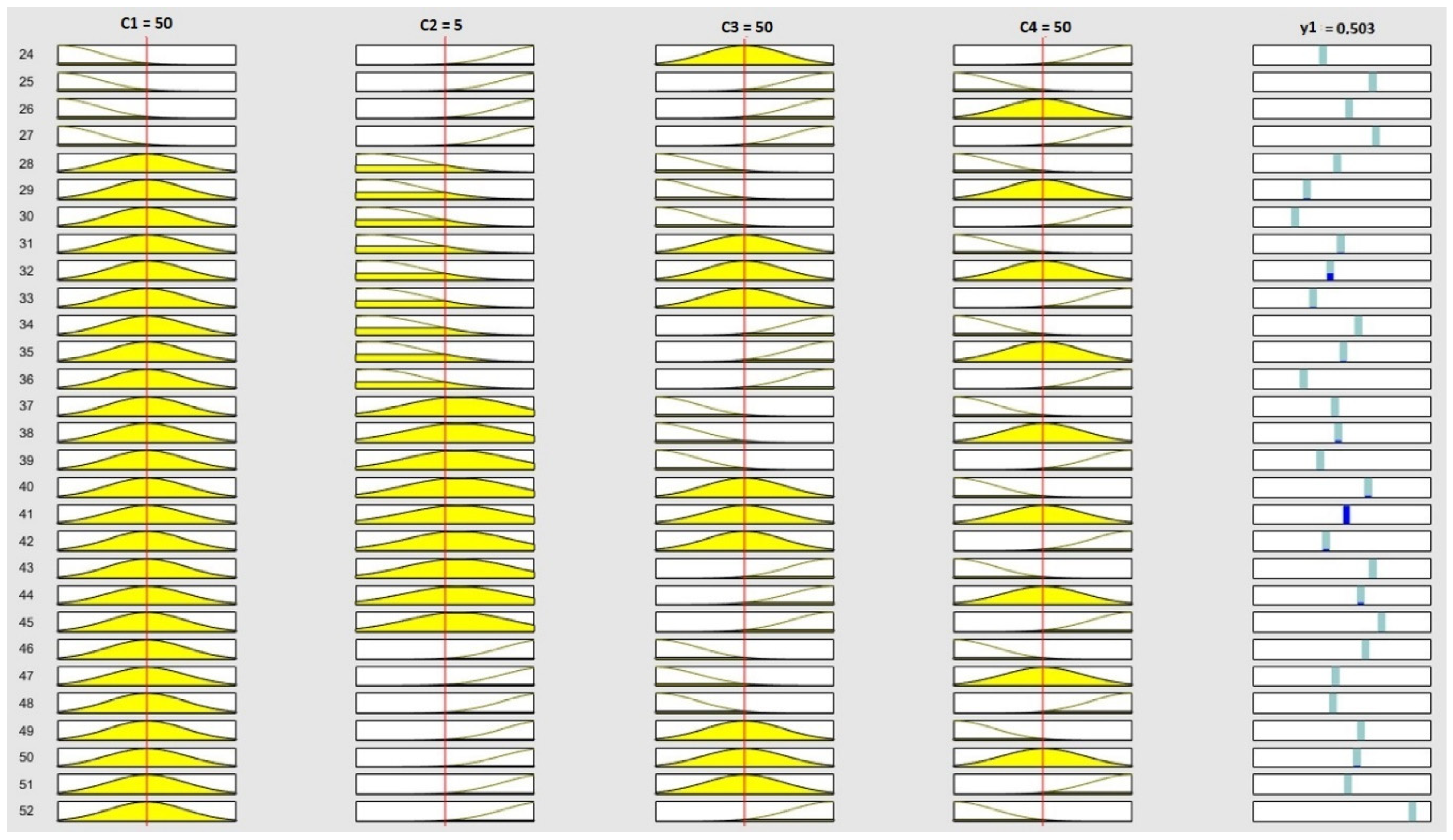
In order to illustrate the effect of the training and the inference process for the ANFIS models, Figure 5 presents part of the 81 decision-making rules for Topology 26 (ANFIS 1 model) before the training processes, while Figure 6 presents the same rules after the training. In these figures, the first four columns represent the input variables and the last represents the output variable. The vertical lines in red represent input values and the parts in yellow represent activated rules. The contribution of each activated rule is represented by the navy blue color in the last column. To illustrate the inference process, we used the input values C1=50, C2=5, C3=50 and C4=50 in this model. Since the consequents of the inference rules in Figure 5 have not been adjusted yet, the output value for each individual rule was 0. Before training, 8 rules were activated, namely rules 14, 32, 38, 41, 42, 44, 50 and 68, generating an output value of 0. After training, with the adjustment in the decision-making rules, 14 rules were activated, namely rules 5, 14, 29, 31, 32, 33, 38, 40, 41, 4, 44, 50, 59 and 68, which achieved an output value of 0.503. In Figure 6, in addition to the changes in the values of the consequents for each rule, we can also observe the effect of changes in the format of some pertinent functions after training. These changes are more evident in the first two functions of Criteria C2 (the environmental management system). Thus, when suppliers have an environmental management system with “low” or “medium” performance, this will influence the Y1 results more strongly than if they were in other environmental criteria with “low” or “medium” performances. This demonstrates the great relevance of this criterion in terms of supplier environmental performance.
Figure 6.
Decision-Making Rules for Candidate Topology #26 before Training.
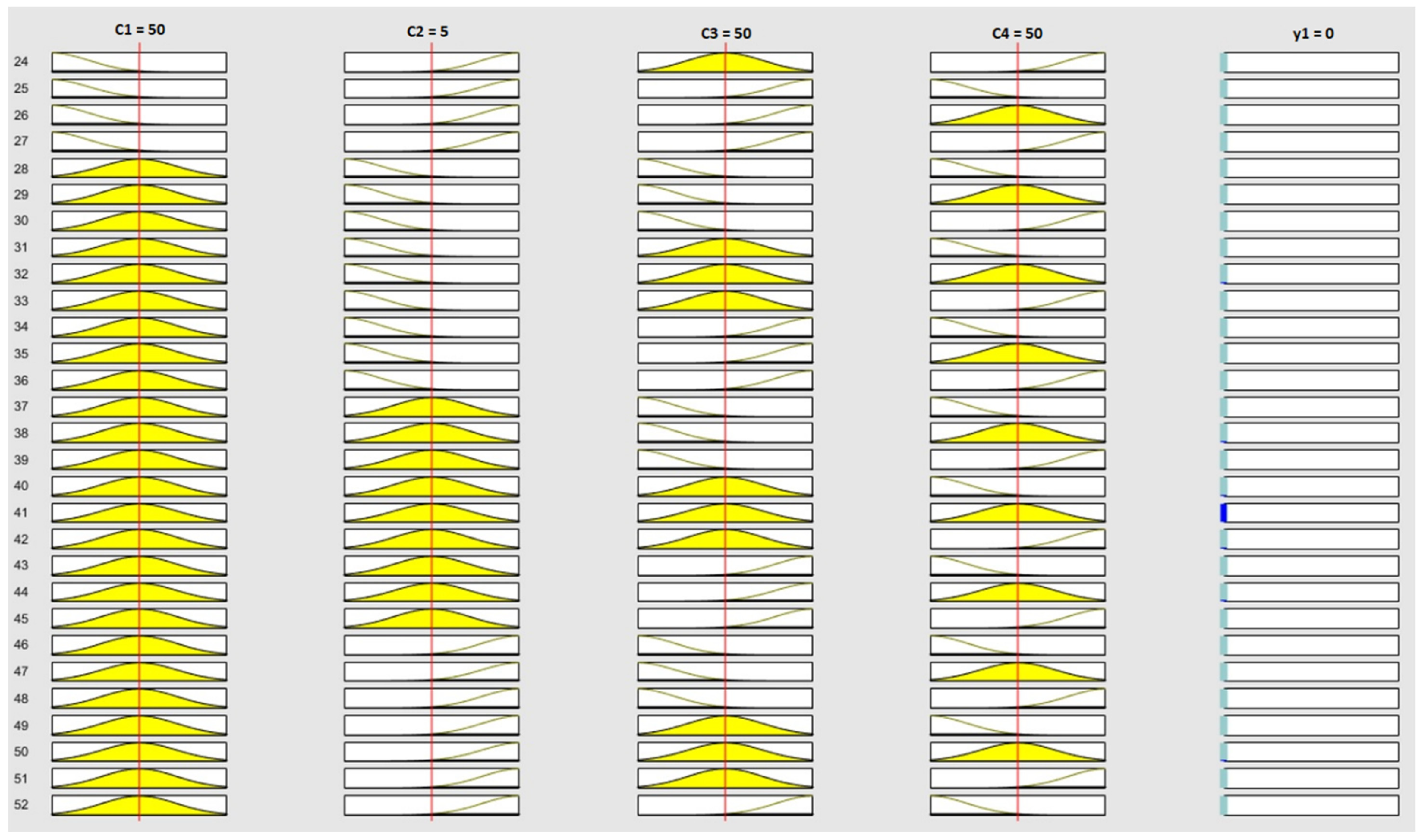
Figure 7.
Decision-Making Rules for Candidate Topology #26 after Training.
In order to show the relationships between some of the input variables and the output variable for each ANFIS model, Figure 8(a) to Figure 8(c) show the response surface graphs produced after training the ANFIS models. In Figure 8(b), it is possible to visualize that Criteria C5 (employment practices) and C7 (local community influence) have a linear relationship with the output variable Y2 if the value of one of these criteria is null. In these cases, an increase of the values of these criteria produces a proportional increase in the value of Y1. On the other hand, in Figure 8(c) it is possible to verify that there is a non-linear relationship between C9 (quality) and Y3. If a supplier achieves "high" performance in quality, the value of Y2 will increase substantially. This indicates that the criterion has great relevance for economic performance.
4.2.3. Stage 3: Supplier Categorization
The last step in applying the proposed model consists of segmenting the suppliers based on the performance values obtained for each ANFIS model in Step 2.3. Threshold values for all of the dimensions were set at 0.5 by the DMs. Figure 9 presents the results of the classification of the 60 suppliers evaluated in the previous stage. To improve the visualization of the suppliers in each quadrant, the matrix has been separated into two parts.
The results presented in Figure 9 indicate that eight suppliers were classified in Group 1 because of their poor performance in all of the matrix’s dimensions. If it is not possible to substitute the suppliers in this group, there are strategies that can be applied to improve their economic, environmental, and social development. Six suppliers were classified in Group 2, and the classification results suggest applying strategies to improve their economic and social development. There were twelve suppliers classified in Group 3, which need strategies to improve their social and environmental development. For Group 4, there were four suppliers whose social performance needs to be improved. For Group 5 there were five suppliers, and they need strategies to improve their economic and environmental development. For Group 6, there were ten suppliers in need of economic development strategies, and for Group 7, there were seven suppliers in need of environmental development strategies. Finally, there are eight suppliers classified in Group 8. These suppliers are the best in the supplier database because they meet the buying company's environmental, social and economic requirements. The results of the supplier classification in the segmentation matrix were endorsed by the DMs.
Finally, with the suppliers separated into the proposed segmentation matrix, we were able to identify and propose specific strategies for each group to increase their sustainability performance. Based on the result analysis and discussions with the DMs, some possible development programs were indicated for each group. Table 4 served as the basis for defining these programs. For example, supplier F5 was classified in the G7 group and presented poor performance in the environmental dimension. This supplier performed poorly on the environmental management system (C2) and resource consumption (C3) criteria. In this case, the DMs have recommended a strategy in which they “help suppliers to obtain ISO1400 certification”. The supplier F30 was classified in the G4 group, with poor performance in the social dimension. Since this supplier achieved low scores in all of the social criteria, the DMs have suggested applying strategies such as “eliminate poor health conditions” and “adopt ethics standards with employees, customers, suppliers and investors”. Therefore, choosing one or more strategies should consider the group in which the supplier has been classified, and should also take into account the criteria where they are underperforming.
4.3. Comparison of the Results with Previous Studies
The proposed model has some advantages in relation to previous supplier segmentation models. Unlike most of the models displayed in Table 3, the proposed model allows the classification of suppliers according to each of the TBL dimensions to provide support for improving supplier sustainability. In comparison with the models for sustainable supplier segmentation proposed by Torres-Ruiz and Ravindran (2018), Rius-Sorolla et al. (2020), Borges et al. (2022), Mavi et al. (2023), Rahiminia et al. (2023), and Taghipour et al. (2023), the proposed approach has the advantage of not performing any compensation between the performance dimensions. In this way, when the performance of a supplier in one dimension is low, even if this same supplier has high performance in two of the TBL dimensions, the final result will point to a performance gap. Thus, the model contributes to identifying suppliers with performance gaps while also aiding in achieving a balance among environmental, social, and economic performance.
Like the supplier segmentation models based on AHP (Rezaei and Ortt, 2013b; Santos et al., 2017; Torres-Ruiz and Ravindran, 2018; Bianchini et al., 2019); ANP (Coşkun et al., 2022), BWM (Rezaei et al., 2015), fuzzy logic (Osiro et al., 2014; Akman, 2015; Medeiros and Ferreira, 2018; Duc et al., 2021; Jharkharia and Das, 2019, Mavi et al., 2023), and rough sets (Bai et al., 2017), the proposed model is appropriate for dealing with decision-making processes under uncertainty. However, unlike techniques based on paired comparisons such as AHP, ANP and Fuzzy AHP, the proposed model does not limit the number of suppliers that can be evaluated simultaneously.
In contrast to artificial neural networks, ANFIS models do not function as black boxes, because their results are more easily interpretable by DMs. Inference rules and surface plots help us understand how the outputs are calculated. Another benefit is that using ANFIS models makes it possible to predict supplier performance values with a high degree of accuracy for each TBL dimension. The accuracy values achieved by the best topologies were in keeping with the findings of other studies which apply ANFIS models for supply chain management. For example, Ozkan and Inal (2014), had higher MSE values with a magnitude of 10-2, while Lima and Carpinetti (2020) achieved lower error values with an MSE value close to a magnitude of 10-16.
5. Statistical Test Results
Linear regression tests were performed to analyze the relationship between the expected output variables and the values predicted by the best topologies. The R² coefficient was calculated to verify the dependent relationship of the y variable (predicted values) with the independent x variable (expected values). R² represents the square of the correlation coefficient. The closer it is to 1, the better the model is adjusted in representing the dependent relationship between the input and output variables (Montgomery and Runger, 2018).
Figure 10(a) to Figure 10(c) show the expressions that indicate the relationships between the x and y variables, the values of R², and the results of the regression tests performed in Microsoft Excel. The values obtained for R2 were 0.9905, 0.9996, and 0.8872 for the ANFIS 1, 2 and 3 models respectively. The predicted values for the ANFIS models are very close to the expected values (validation set). However, the ANFIS 3 model presented the poorest performance among the three analyzed models. This is because it has the most significant number of input variables and therefore has a larger number of inference rules, which implies a more significant number of parameters to be adjusted during the training, which directly interferes with the model’s accuracy.
To verify whether there is a significant difference between the expected values and the predicted values using the ANFIS models, we performed three paired t tests. According to Montgomery and Runger (2018), this type of test is appropriate when the population data is collected in pairs. Table 10 demonstrates the acceptance and rejection criteria for the null hypothesis with a significance level of α.
To perform the t tests, the samples need to fulfill the requirements of a normal distribution and homogeneity for the variances among the groups (Fávero, Belfiore, 2017). The normality and homogeneity tests of the variances were performed using the SPSS Statistics software with groups of 60 samples for each validation step of the three ANFIS models. The significance level of α = 0.1 was defined for the rejection of the null hypothesis, considering the null hypothesis to be that the sample comes from a normal distribution and the alternative hypothesis to be that the sample does not come from a normal distribution. Table 11 presents the results of the normality tests for the six groups of samples, with there being two for each ANFIS model.
As displayed in Table 11, the data’s normality was calculated based on the Shapiro-Wilk (S-W) Test. This test is recommended for samples where 4 < n < 2,000 (Fávero and Belfiore, 2017). The analysis of the test results was performed based on their p-values. Taking into account a level of significance of α = 0.01 and considering that all of the cases presented p-values > α, the null hypotheses of the six sample groups were accepted, or in other words, all of the sample groups in Table 11 come from a normal distribution.
To verify the homogeneity of the variances among the groups, we performed Levene’s Test utilizing the SPSS Statistics software. Compared to other tests of homogeneity, such as Hartley’s Test or the Cochran Test, Levene’s Test is more sensitive to deviations from normality, and it is considered to be the most robust of these tests (Fávero and Belfiore, 2017). Table 12 presents the results achieved by the samples for the ANFIS models for the homogeneity of variance test. With observed levels of significance of 0.728, 0.990, and 0.423, values which are greater than α = 0.01, the test results indicate that the null hypothesis cannot be rejected. Thus, we can conclude that with a confidence level of 99%, that the variances are homogeneous.
Given that the normality and homogeneity of the variance requirements have been achieved, we can apply the t test. Table 13 presents the results obtained by the t tests performed using the SPSS Statistics software. In addition to the levels of significance, Table 13 shows the mean differences between the pairs of each sample group, the standard deviation, the mean standard error, the confidence level of the difference, and the calculated t value. Considering a level of significance of α = 0.01, with the p-values being 0.012, 0.216, and 0.404 for the ANFIS 1, 2, and 3 models respectively, we cannot reject the null hypotheses. Therefore, we conclude that there are no statistically significant differences between the expected values and the predicted values. This reinforces the accuracy of the proposed models and the appropriateness of utilizing ANFIS in sustainable supplier segmentation.
6. Conclusion
This study proposes a model designed to support sustainable supplier segmentation which consists of three adaptive network-based fuzzy inference systems, one for each TBL dimension. The applicability of the proposed model has been demonstrated through its application in a sugarcane mill. The implementation and evaluation of dozens of ANFIS topologies has made it possible to identify the most suitable values for the internal parameters of the models. The linear regression analysis and the R² indicated a high positive correlation between the expected values and the values predicted by the models. The hypothesis tests indicate that there were no significant differences between the expected values and the predicted values for the ANFIS models.
In terms of its practical contributions, the proposed model has proven to be a useful tool in supporting managers in sustainable supplier segmentation processes designed to promote a more sustainable supply chain. It can help managers analyze the performance of their suppliers and identify aspects that need to be improved. The use of a machine learning-based approach has proven to be a more sophisticated solution for supporting supplier segmentation. The results provided by the model are useful in supporting DMs in the definition of specific development strategies for each supplier group. Since it does not use a compensatory decision-making approach, the three TBL dimensions are given equal importance in the elaboration of actions designed to improve supplier performance, thus avoiding the problems associated with the compensation effect.
The proposed model in this study also has several advantages over previous supplier segmentation models identified in the literature. In addition to the benefits discussed in Section 3.3, this proposal presents the following contributions to the supplier segmentation literature:
- By using a supervised learning method, this is the first supplier segmentation model that enables the use of historical performance data to automatically adjust the relationships between the variables. The use of ANFIS requires less training time to adjust its internal parameters than models based on neural networks or fuzzy inference;
- Due to its use of fuzzy input variables and fuzzy inference rules, this model is appropriate for supporting decision making based on DM judgments or imprecise numerical values. Another advantage is that it enables the use of both quantitative and qualitative criteria, which is essential in assessing social performance;
- The supervised learning process makes it possible to incorporate the available knowledge about supplier performance into the inference rules. This makes the results produced by the ANFIS models easily interpretable and makes it possible to identify which decision rules produced the results. The response surface graphs also contribute to a better understanding of the cause-and-effect relationships between the input variables and the output variable. Thus, transparency in the processing of information helps decision makers feel more secure in justifying their decisions.
Another contribution of this study is its identification of appropriate topological parameters to obtain more accurate results, which can help researchers and developers in the creation of computation solutions based on ANFIS for supplier evaluation. A limitation of this study is that only one training algorithm has been tested in the cross-reference validation process. We opted to just test the algorithm which was most frequently applied in ANFIS training, because it achieved satisfactory accuracy in most of the applications found in the literature (Lima and Carpinetti, 2020). To test each additional algorithm would require constructing 108 additional topologies each time, which would make the modeling process excessively lengthy and may threaten the viability of the application of the proposed model. Future studies can test other supervised learning methods in the supplier segmentation process. It would also be useful to conduct comparative studies of the supplier segmentation models displayed in Table 3. Furthermore, we suggest the application of the proposed model in companies within the TBL context operating in other economic sectors.
Funding
This study was financed by the Coordinating Body for the Improvement of Higher Education Personnel (CAPES) – Finance Code 001.
Acknowledgments
We would like to thank the employees of the company where the application took place. We would also like to thank the anonymous reviewers for their contributions which have improved this work.
References
- Ahi, P.; Searcy, C. An analysis of metrics used to measure performance in green and sustainable supply chains; Journal of Cleaner Production, 2015; Vol. 86, pp. 360–377. [Google Scholar]
- Akkoç, S. An empirical comparison of conventional techniques, neural networks and the three stages hybrid Adaptive Neuro Fuzzy Inference System (ANFIS) model for credit scoring analysis: The case of Turkish credit card data; European Journal of Operational Research, 2012; Vol. 222, No 1, pp. 168–178. [Google Scholar]
- Akman, G. Evaluating suppliers to include green supplier development programs via fuzzy c-means and VIKOR methods; Computers & Industrial Engineering, 2015; Vol. 86, pp. 69–82. [Google Scholar]
- Aloini, D.; Dulmin, R.; Mininno, V.; Zerbino, P. Leveraging procurement related knowledge through a fuzzy-based DSS: a refinement of purchasing portfolio models; Journal of Knowledge Management, 2019; Vol. 23, No 6, pp. 1077–1104. [Google Scholar]
- Bai, C.; Kusi-Sarpong, S.; Khan, S.A.; Vazquez-Brust, D. Sustainable buyer–supplier relationship capability development: a relational framework and visualization methodology; Annals of Operations Research, 2021; Vol. 304, pp. 1–34. [Google Scholar]
- Bai, C.; Rezaei, J.; Sarkis, J. Multicriteria green supplier segmentation; IEEE Transactions on Automation Science and Engineering, 2017; Vol. 64, No 4, pp. 515–528. [Google Scholar]
- Bamakan, S.M.H.; Faregh, N.; ZareRavasan, A. Di-ANFIS: an integrated blockchain–IoT–big data-enabled framework for evaluating service supply chain performance; Journal of Computational Design and Engineering, 2021; Vol. 8, No 2, pp. 676–690. [Google Scholar]
- Bianchini, A.; Benci, A.; Pellegrini, M.; Rossi, J. Supply chain redesign for lead-time reduction through Kraljic purchasing portfolio and AHP integration; Benchmarking: An International Journal, 2019; Vol. 26, No 4, pp. 1194–1209. [Google Scholar]
- Borges, W.V.; Lima, F.R.; Junior. Decision Support Models for Supplier Segmentation: A Systematic Literature Review. In Proceedings of the Brazilian Congress of Production Engineering (CONBREPRO), Brazil; 2020. [Google Scholar]
- Borges, W.V.; Lima, F.R.; Junior; Peinado, J.; Carpinetti, L.C.R. A Hesitant Fuzzy Linguistic TOPSIS model to support Supplier Segmentation; Journal of Contemporary Administration, 2022; Vol. 26, p. e210133. [Google Scholar]
- Boujelben, M.A. A unicriterion analysis based on the PROMETHEE principles for multicriteria ordered clustering; Omega, 2017; Vol. 69, pp. 126–140. [Google Scholar]
- Coşkun, S.S; Kumru, M.; Kan, N.M. An integrated framework for sustainable supplier development through supplier evaluation based on sustainability indicators; Journal of Cleaner Production, 2022; Vol. 335, p. 130287. [Google Scholar]
- Day, M.; Magnan, G.M.; Moeller, M.M. Evaluating the bases of supplier segmentation: a review and taxonomy; Industrial Marketing Management, 2010; Vol. 39, No 4, pp. 625–639. [Google Scholar]
- Demir, L.; Akpinar, M.E.; Araz, C.; Ilgin, M.A. A green supplier evaluation system based on a new multi-criteria sorting method: VIKORSORT; Expert Systems with Applications, 2018; Vol. 114, pp. 479–487. [Google Scholar]
- Duc, D.A.; Van, L.H.; Yu, V.F.; Chou, S.Y.; Hien, N.V.; Chi, N.T.; Toan, D.V.; Dat, L.Q. A dynamic generalized fuzzy multi-criteria group decision making approach for green supplier segmentation; Plos One, 2021; Vol. 16. [Google Scholar]
- Fávero, L.P.; Belfiore, P. Manual de análise de dados: estatística e modelagem multivariada com Excel, SPSS e Stata; Rio de Janeiro; Elsevier, 2017. [Google Scholar]
- Finger, G.W.S.; Lima, F.R.; Junior. A hesitant fuzzy linguistic QFD approach for formulating sustainable supplier development programs; International Journal of Production Economics, 2022; Vol. 247, p. 108428. [Google Scholar]
- Haghighi, P.S.; Moradi, M.; Salahi, M. Supplier Segmentation using fuzzy linguistic preference relations and fuzzy clustering; International Journal of Intelligent Systems and Applications, 2014; Vol. 6, pp. 76–82. [Google Scholar]
- Jang, J-S.R. ANFIS: adaptive-network-based fuzzy inference system; IEEE Transactions on Systems, 1993; Vol. 23, No 3, pp. 665–685. [Google Scholar]
- Jharkharia, S.; Das, C. Low carbon supplier development: a fuzzy c-means and fuzzy formal concept analysis based analytical model; Benchmarking: An International Journal, 2019; Vol. 26, No 1, pp. 73–96. [Google Scholar]
- Kaur, H.; Singh, S.P. Multi-stage hybrid model for supplier selection and order allocation considering disruption risks and disruptive technologies; International Journal of Production Economics, 2021; Vol. 231, p. 107830. [Google Scholar]
- Keskin, F.D.; Kaymaz, Y.; Unvan, Y.A. "Machine learning in supply chain management: a risk-based supplier segmentation application". In Business studies and new approaches; Lyon; Livre de Lyon, 2021; pp. 139–161. [Google Scholar]
- Lajimi, H.F.; "Sustainable supplier segmentation: a practical procedure"; Rezaei, J. Strategic Decision Making for Sustainable Management of Industrial Networks; Cham; Springer, 2021; pp. 119–137. [Google Scholar]
- Li, Y.; et al. Multi-criteria group decision analytics for sustainable supplier relationship management in a focal manufacturing company; Journal of Cleaner Production, 2024; Vol. 476, p. 143690. [Google Scholar]
- Lima, F.R.; Junior; Oliveira, M.E.B.; Resende, C.H.L. An Overview of Applications of Hesitant Fuzzy Linguistic Term Sets in Supply Chain Management: The State of the Art and Future Directions; Mathematics, 2023; Vol. 11. [Google Scholar]
- Lima, F.R.; Junior; Carpinetti, L.C.R. Combining SCOR® model and fuzzy TOPSIS for supplier evaluation and management; International Journal of Production Economics, 2016; Vol. 174, pp. 128–141. [Google Scholar]
- Lima, F.R.; Junior; Carpinetti, L.C.R. An adaptive network-based fuzzy inference system to supply chain performance evaluation based on SCOR® metrics; Computers & Industrial Engineering, 2020; Vol. 139, p. 106191. [Google Scholar]
- Lo, S.C.; Sudjatmika, F.V. Solving multi-criteria supplier segmentation based on the modified FAHP for supply chain management: a case study; Soft Computing, 2016; Vol. 20, pp. 4981–4990. [Google Scholar]
- Matshabaphala, N.M.; Grobler, J. Supplier segmentation: a case study of Mozambican cassava farmers; The South African Journal of Industrial Engineering, 2021; Vol. 32, No 1, pp. 196–209. [Google Scholar]
- Mavi, R.K.; Zarbakhshnia, N.; Mavi, N.K.; Kazemi, S. Clustering sustainable suppliers in the plastics industry: A fuzzy equivalence relation approach; Journal of Environmental Management, 2023; Vol. 345, p. 118811. [Google Scholar]
- Mavi, R.K.; Mavi, N.K.; Goh, M. Modeling corporate entrepreneurship success with ANFIS; Operational Research, 2017; Vol. 17, pp. 213–238. [Google Scholar]
- Medeiros, M.; Ferreira, L. Development of a purchasing portfolio model: an empirical study in a Brazilian hospital; Journal Production Planning & Control, 2018; Vol. 29, No 7, pp. 571–585. [Google Scholar]
- Montgomery, D.; Runger, G. Applied statistics and probability for engineers; Hoboken: Wiley, 2018. [Google Scholar]
- Osiro, L.; Lima, F.R.; Junior; Carpinetti, L.C.R. A fuzzy logic approach to supplier evaluation for development; International Journal of Production Economics, 2014; Vol. 153, pp. 95–112. [Google Scholar]
- Özkana, G.; Inal, M. Comparison of neural network application for fuzzy and ANFIS approaches for multi-criteria decision-making problems; Applied Soft Computing, 2014; Vol. 24, pp. 232–238. [Google Scholar]
- Parkouhi, S.V.; Ghadikolaei, A.S.; Lajimi, H.F. Resilient supplier selection and segmentation in grey environment; Journal of Cleaner Production, 2019; Vol. 207, pp. 1123–1137. [Google Scholar]
- Paybarjay, H.; Lajimi, H.F.; Zolfani, S.H. An investigation of supplier development through segmentation in sustainability dimensions; Environment, Development and Sustainability, 2023. [Google Scholar]
- Pedroso, C.B.; Tate, W.L.; Silva, A.L.; Carpinetti, L.C.R. Supplier development adoption: A conceptual model for triple bottom line (TBL) outcomes; Journal of Cleaner Production, 2021; Vol. 314, p. 127886. [Google Scholar]
- Rahiminia, M.; Razmi, J.; Shahrabi Farahani, S.; Sabbaghnia, A. Cluster-based supplier segmentation: a sustainable data-driven approach; Modern Supply Chain Research and Applications, 2023; Vol. 5, No 3, pp. 209–228. [Google Scholar]
- Rajesh, G.; Raju, R. A fuzzy inference approach to supplier segmentation for strategic development; The South African Journal of Industrial Engineering, 2021; Vol. 32, No 1, pp. 44–55. [Google Scholar]
- Rashidi, K.; Noorizadeh, A.; Kannan, D.; Cullinane, K. Applying the triple bottom line in sustainable supplier selection: a meta-review of the state-of-the-art; Journal of Cleaner Production, 2020; Vol. 269, p. 122001. [Google Scholar]
- Resende, C.H.L.; Lima, F.R.; Junior; Carpinetti, L.C.R. Decision-making models for formulating and evaluating supplier development programs: a state-of-the-art review and research paths; Transportation Research Part E-Logistics and Transportation Review, 2023; Vol. 180, p. 103340. [Google Scholar]
- Restrepo, R.; Villegas, J.G. Supplier evaluation and classification in a Colombian motorcycle assembly company using data envelopment analysis; Academia Revista Latinoamericana de Administración, 2019; Vol. 32, No 2, pp. 159–180. [Google Scholar]
- Rezaei, J.; Kadzinski, M.; Vana, C.; Tavasszy, L. Embedding carbon impact assessment in multi-criteria supplier segmentation using ELECTRE TRI-rC", Annals of Operations Research, 2017.
- Rezaei, J.; Lajimi, H.F. Segmenting supplies and suppliers: bringing together the purchasing portfolio matrix and the supplier potential matrix; International Journal of Logistics Research and Applications, 2019; Vol. 22, No 4, pp. 419–436. [Google Scholar]
- Rezaei, J.; Ortt, R. Multi-criteria supplier segmentation using a fuzzy preference relation based AHP; European Journal of Operational Research, 2013a; Vol. 225, No 1, pp. 75–84. [Google Scholar]
- Rezaei, J.; Ortt, R. Supplier segmentation using fuzzy logic; Industrial Marketing Management, 2013b; Vol. 42, No 4, pp. 507–517. [Google Scholar]
- Rezaei, J.; Wang, J.; Tavasszy, L. Linking supplier development to supplier segmentation using Best Worst Method; Expert Systems with Applications, 2015; Vol. 42, No 23, pp. 9152–9164. [Google Scholar]
- Rius-Sorolla, G.; Estelles-Miguel, S.; Rueda-Armengot, C. Multivariable supplier segmentation in sustainable supply chain management; Sustainability, 2020; Vol. 12, No 11. [Google Scholar]
- Santos, L.F.O.M; Osiro, L.; Lima, R.H.P. A model based on 2-tuple fuzzy linguistic representation and Analytic Hierarchy Process for supplier segmentation using qualitative and quantitative criteria; Expert Systems with Applications, 2017; Vol. 79, pp. 53–64. [Google Scholar]
- Schramm, V.B.; Cabral, L.P.B.; Schramm, F. Approaches for supporting sustainable supplier selection-A literature review; Journal of Cleaner Production, 2020; Vol. 273, p. 123089. [Google Scholar]
- Segura, M.; Maroto, C. A multiple criteria supplier segmentation using outranking and value function methods; Expert Systems with Applications, 2017; Vol. 69, pp. 87–100. [Google Scholar]
- Shiralkar, K.; Bongale, A.; Kumar, S. Nos with decision making methods for supplier segmentation in supplier relationship management: a literature review; Materials Today: Proceedings, 2022; Vol. 50, No 5, pp. 1786–1792. [Google Scholar]
- Silva, I.N.; Spati, D.H.; Flauzino, R.A. Redes neurais artificiais: para engenharia e ciências aplicadas; São Paulo; Artliber, 2016. [Google Scholar]
- Subramanian, N.; Gunasekaran, A. Cleaner supply-chain management practices for twenty-first-century organizational competitiveness: Practice-performance framework and research propositions; International Journal of Production Economics, 2015; Vol. 164, pp. 216–233. [Google Scholar]
- Taghipour, A.; Fooladvand, A.; Khazaei, M.; Ramezani, M. Criteria Clustering and Supplier Segmentation Based on Sustainable Shared Value Using BWM and PROMETHEE; Sustainability, 2023; Vol. 15. [Google Scholar]
- Torres-Ruiz, A.; Ravindran, R. Multiple Criteria Framework for the Sustainability Risk Assessment of a Supplier Portfolio; Journal of Cleaner Production, 2018; Vol. 172, pp. 4478–4493. [Google Scholar]
- Zimmer, K.; Fröhling, M.; Schultmann, F. Sustainable supplier management a review of models supporting sustainable supplier selection, monitoring and development; International Journal of Production Research, 2016; Vol. 54, No 5, pp. 1412–144. [Google Scholar]
Figure 1.
Structure of the ANFIS Model with Three Input Variables.
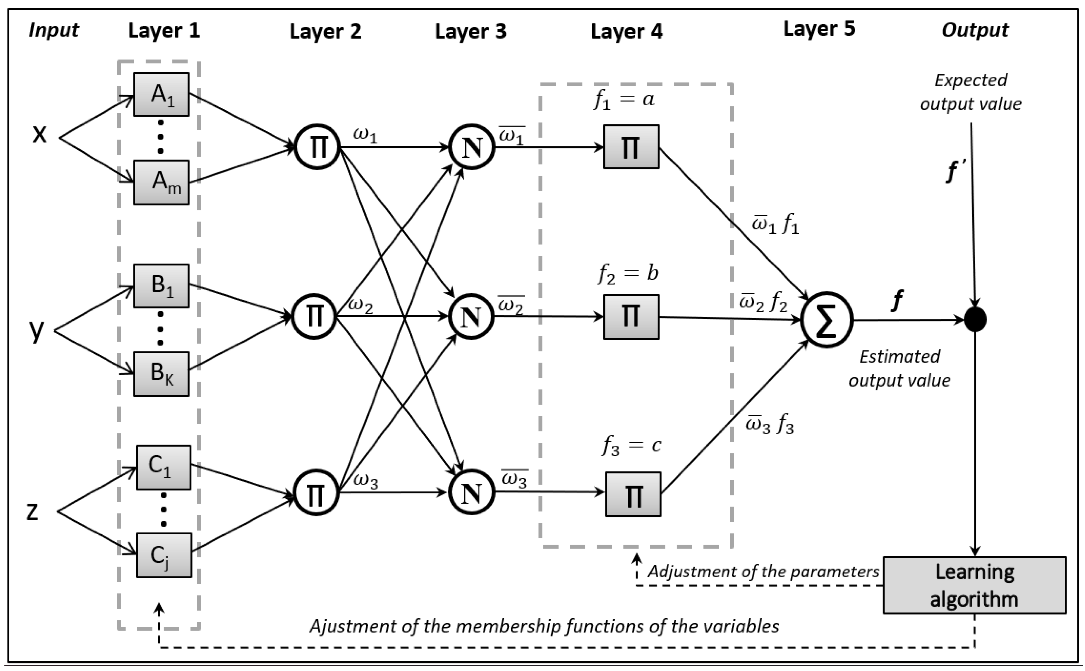
Figure 2.
Proposed Model for Sustainable Supplier Segmentation.
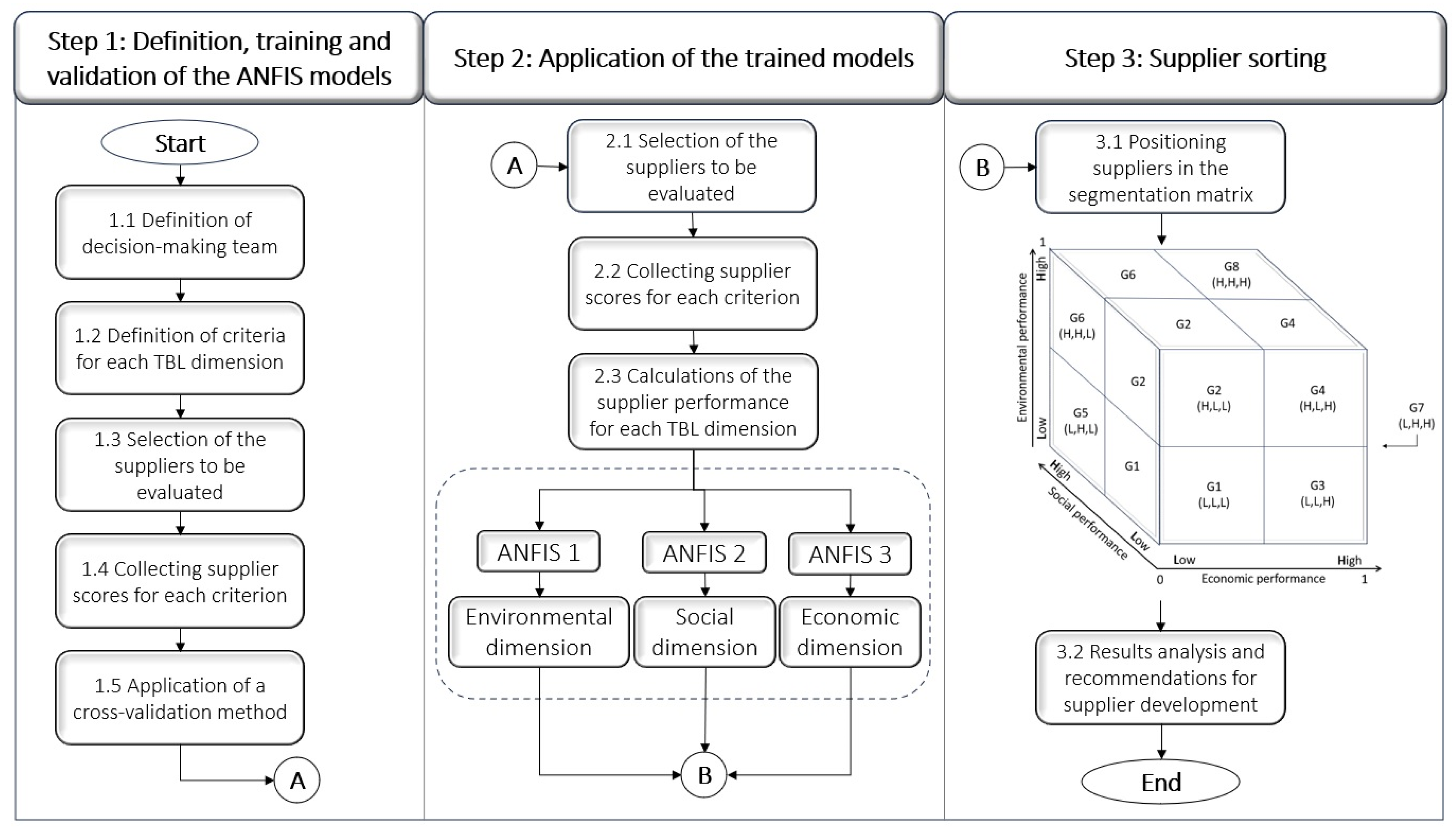
Figure 3.
Cross-Validation Steps for Modeling ANFIS Systems.
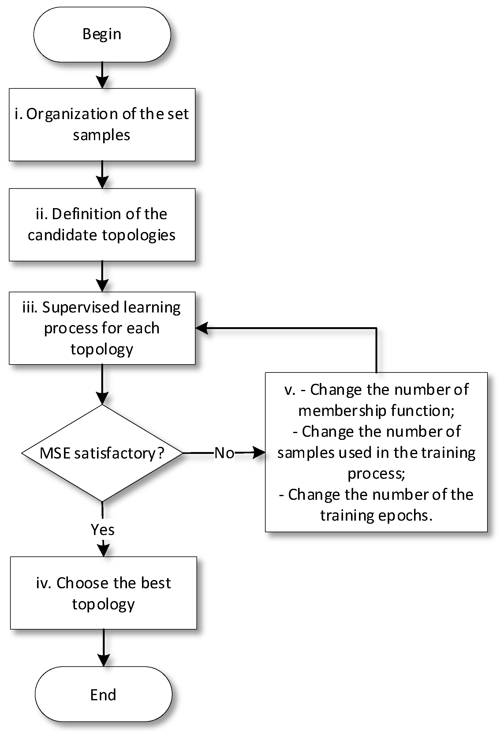
Figure 4.
The Proposed Sustainable Supplier Segmentation Matrix.
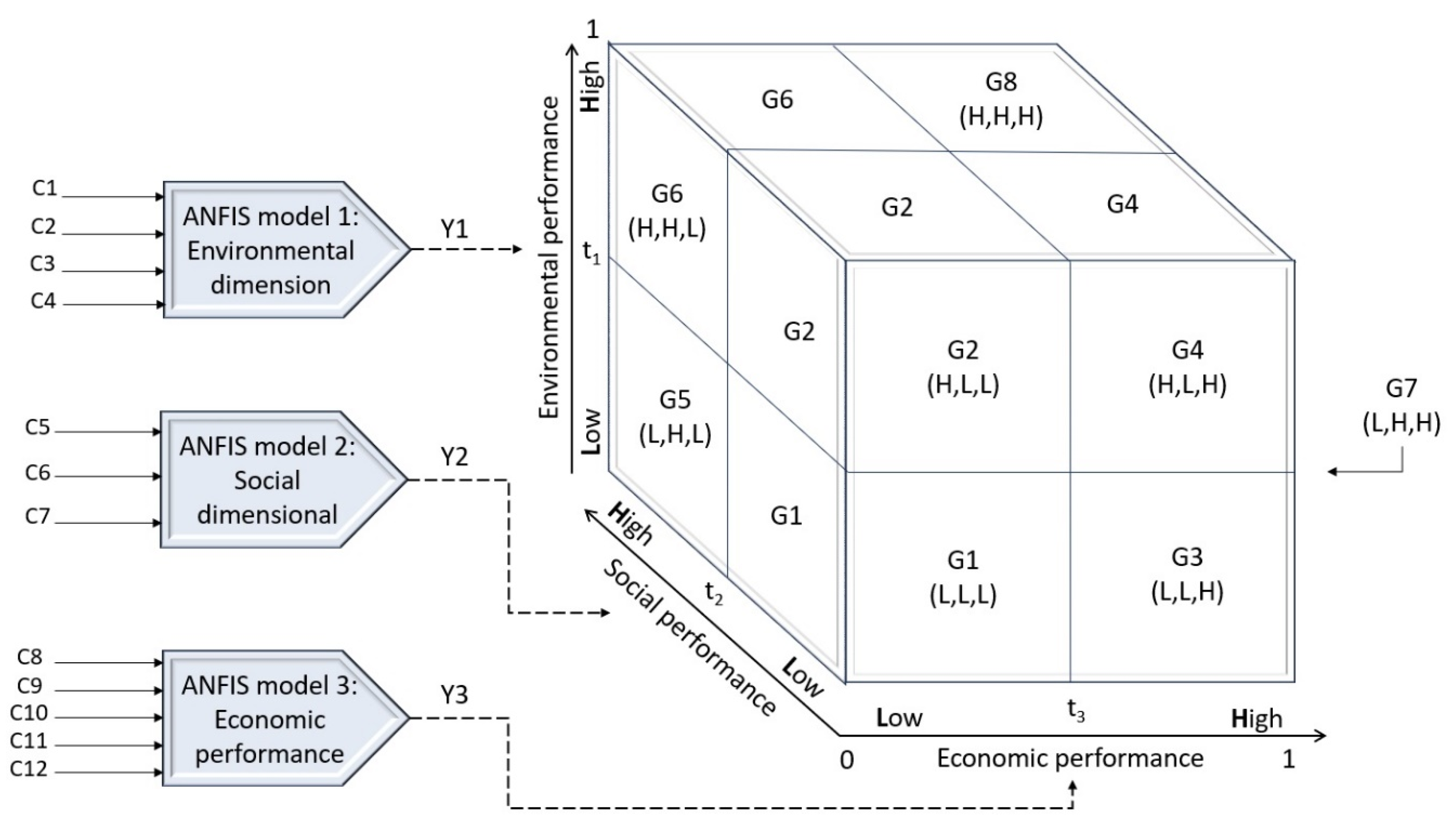
Figure 5.
Comparison of the Predicted Values with the Expected Values for the (a) ANFIS 1, (b) ANFIS 2, (c) ANFIS 3 Models.
Figure 5.
Comparison of the Predicted Values with the Expected Values for the (a) ANFIS 1, (b) ANFIS 2, (c) ANFIS 3 Models.
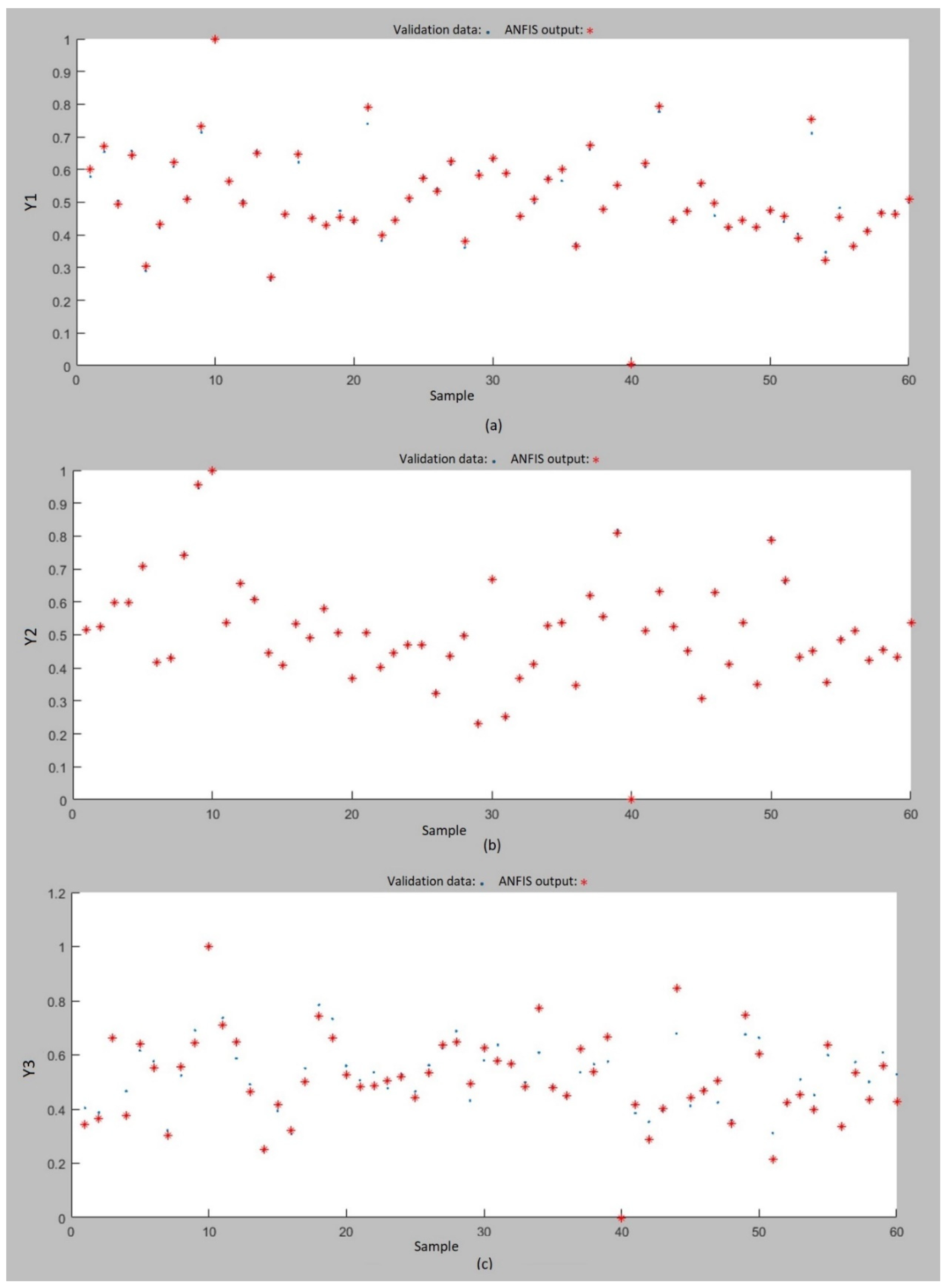
Figure 8.
Response Surface Plots of the (a) ANFIS 1, ANFIS 2 (b), and ANFIS 3 (c) Models.
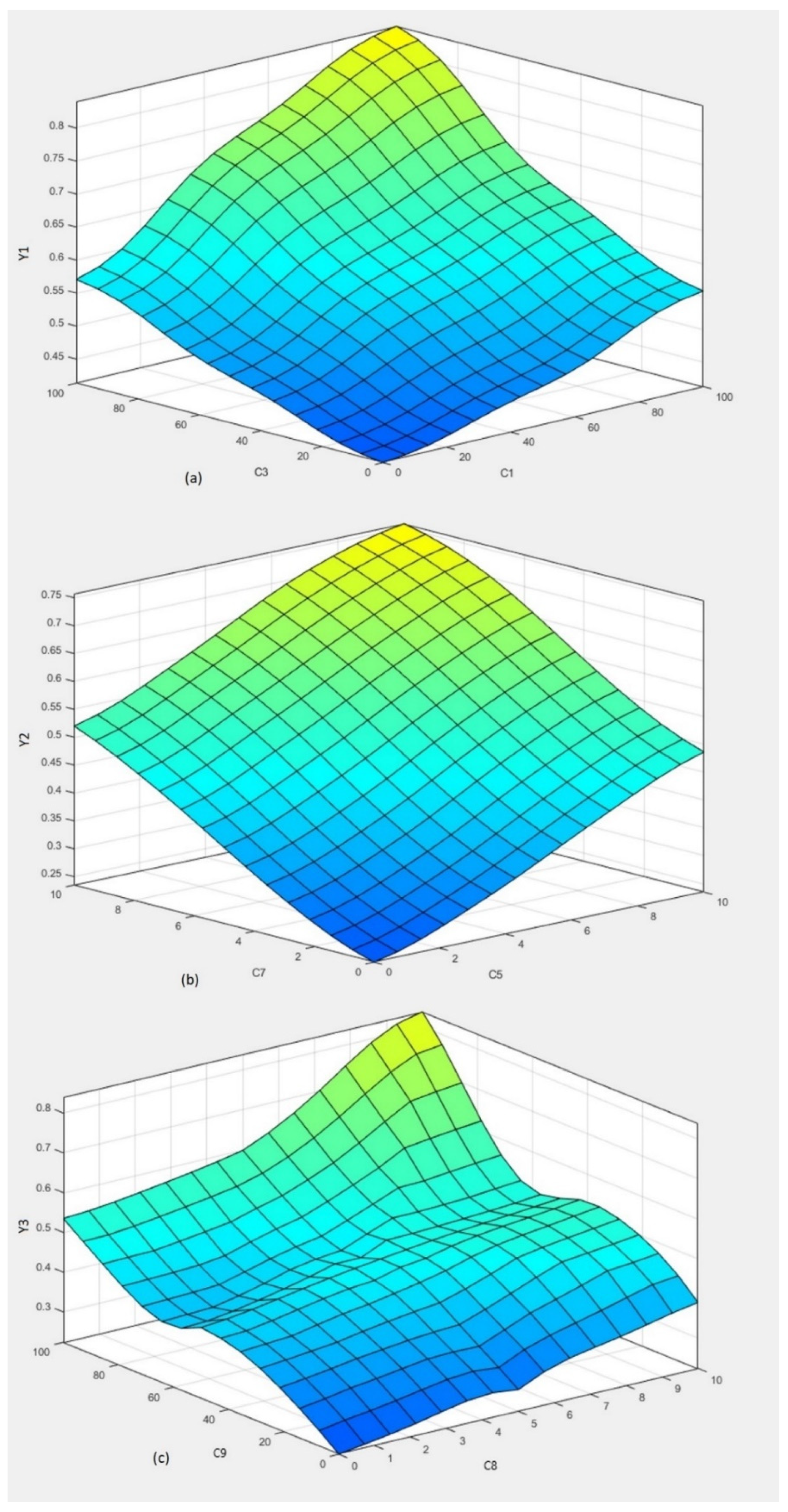
Figure 9.
Final Supplier Classification.
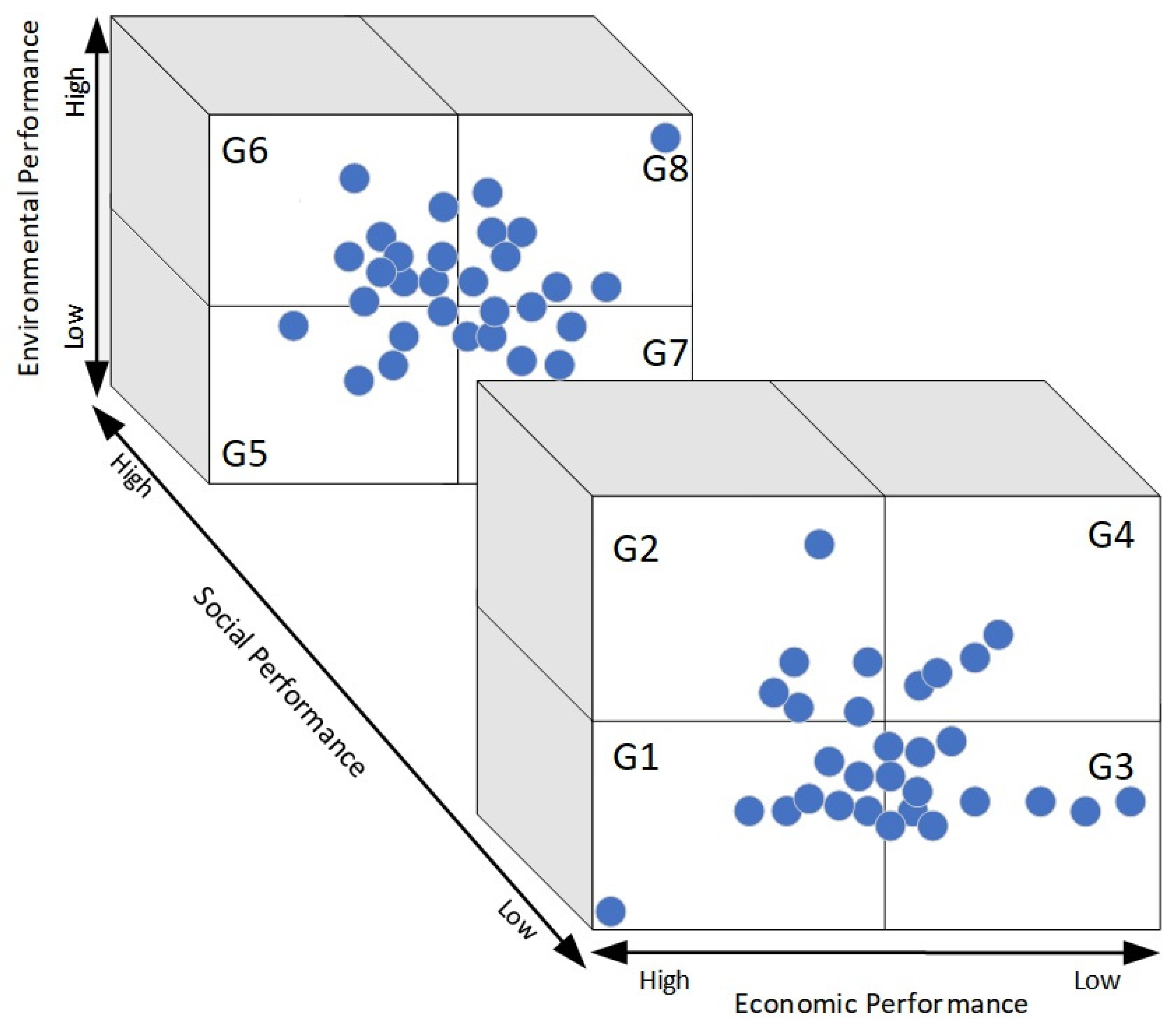
Figure 10.
Results of the Linear Regressions Using the ANFIS 1(a), 2(b) and 3(c) Model Results.
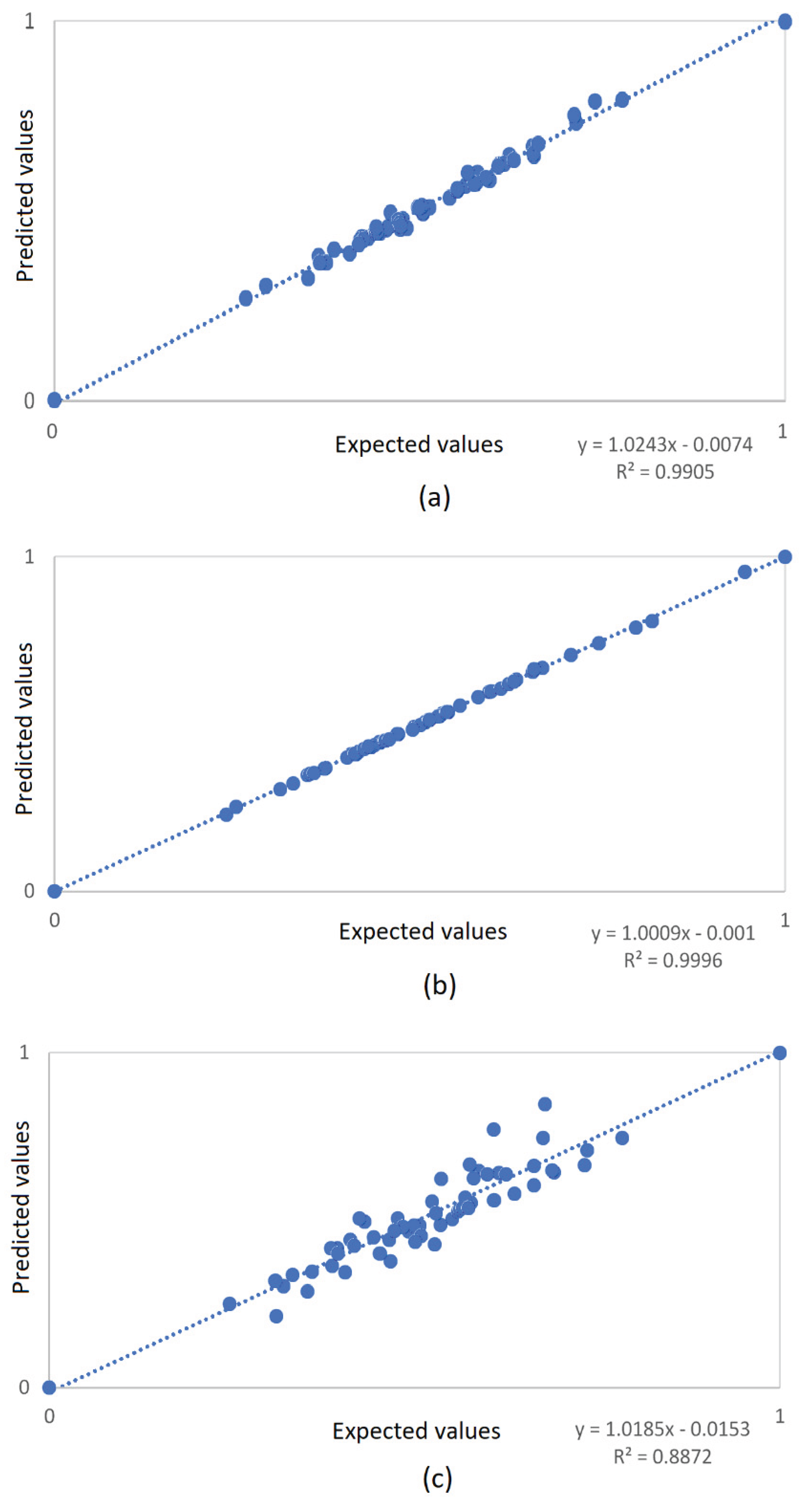

Table 1.
This Study’s Contributions in Comparison to Previous Supplier Segmentation Models.
| Torres-Ruiz and Ravindran (2018) | Rius-Sorolla et al. (2020) | Borges et al. (2022) | Coşkun et al. (2022) | Mavi et al. (2023) | Paybarjay et al. (2023) | Rahiminia et al. (2023) | Taghipour et al. (2023) | Li et al. (2024) | Other studies found in the literature (Table 2) | Our Study | |
|---|---|---|---|---|---|---|---|---|---|---|---|
| Does it offer support for sustainable supplier segmentation? | Yes | Yes | Yes | Yes | Yes | Yes | Yes | Yes | Yes | No | Yes |
| Does it have a supervised learning process? | No | No | No | No | No | No | No | No | No | No | Yes |
| Is segmentation based on economic, environmental and social dimensions? | No | No | No | Yes | Yes | Yes | No | No | Yes | No | Yes |
| Is there compensation among the TBL criteria? | Yes | Yes | Yes | No | Yes | No | Yes | Yes | No | N/A | No |
| Does it have the capacity to model non-linear relationships between input and output variables? | No | No | No | No | No | No | No | No | No | Most do not, with the exception of the models based on fuzzy inference | Yes |
| Does it deal with uncertainty in the decision-making process? | Yes | No | Yes | Partially | Yes | Yes | No | Yes | No | Some of the studies deal with it. | Yes |
Table 2.
Sustainable Supplier Evaluation Criteria.
| Economic criteria | Environmental criteria | Social criteria |
|---|---|---|
| After-sales support (Rezaei and Lajimi, 2019) Communication (Zimmer et al., 2016) Cost (Resende et al., 2023) Delivery time (Rius-Sorolla et al., 2020) Financial capabilities (Borges et al., 2022) Flexibility (Resende et al., 2023) Geographic location (proximity) (Rezaei and Lajimi, 2019) Innovation (Finger and Lima, 2022) Long-term relationship (Rezaei and Lajimi, 2019) Quality (Lajimi, 2021) Research and development (Kar, 2015) Supply chain resilience (Büyükozkan et al., 2017) Service capabilities (Lajimi, 2021) Technological Capability (Rius-Sorolla et al., 2020) |
Biodiversity and ecological impacts (Büyükozkan and Karabulut, 2017) Emissions control (Resende et al., 2023) Energy efficiency (Bai et al., 2017) Environmental certifications (Borges et al. 2022) Environmental management system (Lajimi, 2021) Environmental policies and audits (Ahi and Searcy, 2015) Green packaging (Bai et al., 2017) Green product design (Resende et al., 2023) Recycling programs (Demir et al., 2018) Resource consumption (Resende et al., 2023) Water consumption (Finger and Lima, 2022) Waste management (Resende et al., 2023) |
Child labor (Zimmer et al., 2016) Egalitarian labor sources (Lajimi, 2021) Discrimination (Zimmer et al., 2016) Diversity (Zimmer et al., 2016) Employee satisfaction (Ahi and Searcy, 2015) Employment practices (Lajimi, 2021) Ethical standards (Rezaei and Lajimi, 2019) Health and safety (Finger and Lima, 2022) Human capital investment (Subramanian and Gunasekaran, 2015) Influence of the local community (Resende et al., 2023) Job opportunities (Lajimi, 2021) Supporting educational institutions (Ahi and Searcy, 2015) Supporting community projects (Ahi and Searcy, 2015) |
Table 3.
Previous Decision Models to Support Supplier Segmentation.
| Author(s) | Decision-making techniques | Segmentation dimensions | Supply Chain Management Strategy | ||||
|---|---|---|---|---|---|---|---|
| Traditional | Green | Agile | Resilient | Sustainable | |||
| Akman (2015) | Fuzzy c-means and VIKOR (Vlsekriterijumska Optimizacija I KOmpromisno Resenje in Serbian) | Does not adopt segmentation dimensions | X | ||||
| Aloini et al. (2019) | Fuzzy inference | Supplier attractiveness and strength of the relationship | X | ||||
| Bai et al. (2017) | Rough Sets, VIKOR and fuzzy c-means | Supplier capabilities and willingness | X | ||||
| Bianchini et al. (2019) | AHP | Profit impact and supply risk | X | ||||
| Borges et al. (2022) | Hesitant Fuzzy-TOPSIS (Technique for Order of Preference by Similarity to the Ideal Solution) | Supplier capabilities and willingness | X | ||||
| Boujelben (2017) | PROMETHEE (Preference Ranking Organization Method for Enrichment Evaluation) | Supplier capabilities and willingness | X | ||||
| Coşkun et al. (2022) | ANP (Analytic Network Process), PROMETHEE, and cluster analysis | Economic, environmental, and social | |||||
| Demir et al. (2018) | VIKORSORT | Does not adopt segmentation dimensions | X | ||||
| Duc et al. (2021) | Fuzzy logic | Supplier capabilities and willingness | X | ||||
| Haghighi et al. (2014) | Fuzzy-AHP and Fuzzy c-means | Supplier capabilities and willingness | X | ||||
| Jharkharia and Das (2019) | Fuzzy c-means and Fuzzy formal concept analysis | Supplier investment decisions and supplier collaboration decisions | X | ||||
| Kaur and Singh (2020) | DEA (Data Envelopment Analysis) | Does not adopt segmentation dimensions | X | ||||
| Keskin and Kaymanz (2021) | K-means | Does not adopt segmentation dimensions | X | ||||
| Li et al. (2024) | Bayesian best-worst method and Canopy-K-Means clustering algorithm | Economic, environmental, and social | X | ||||
| Lima and Carpinetti (2016) | Fuzzy-TOPSIS | Cost and delivery performance | X | ||||
| Lo and Sudjatmika (2016) | Fuzzy-AHP | Supplier capabilities and willingness | X | ||||
| Matshabaphala and Grobler (2021) | K-means | Does not adopt segmentation dimensions | X | ||||
| Mavi et al. (2023) | Fuzzy-AHP and Fuzzy equivalence relation | Economic, environmental, social, and risk | X | ||||
| Medeiros and Ferreira (2018) | Fuzzy-TOPSIS | Profit impact and supply risk | X | ||||
| Osiro et al. (2014) | Fuzzy inference | Potential for partnership and delivery performance | X | ||||
| Parkouhi et al. (2019) | Grey DEMATEL (Decision Making Trial and Evaluation Laboratory) and grey simple additive weighting technique | Resiliency enhancer and resiliency reducer | X | ||||
| Paybarjay et al. (2023) | BWM (Best–Worst Method) and Grey SAW (Grey Simple Additive Weighting) | Economic, environmental and social | X | ||||
| Rahiminia et al. (2023) | BWM and K-means | Profit impact and supply risk | X | ||||
| Rajesh and Raju (2021) | Fuzzy inference | Agility capability and business excellence | X | ||||
| Restrepo and Villegas (2019) | DEA | Diversity efficiency and cross efficiency | X | ||||
| Rezaei and Lajimi (2019) | BWM (Best Worst Method) | Supplier capabilities and supplier willingness | X | ||||
| Rezaei and Ortt (2013a) | Fuzzy preference relation based AHP | Supplier capabilities and supplier willingness | X | ||||
| Rezaei and Ortt (2013b) | AHP | Supplier capabilities and supplier willingness | X | ||||
| Rezaei et al. (2017) | ELECTRE (ÉLimination Et Choix Traduisant la REalité, in French) TRI-rC | Supplier capabilities and supplier willingness | X | ||||
| Rezaei et al. (2015) | BWM | Supplier capabilities and supplier willingness | X | ||||
| Rius-Sorolla et al. (2020) | Procedure based on arithmetic mean | Profit impact and supply risk | X | ||||
| Santos et al. (2017) | AHP and Fuzzy 2-tuple | Supplier capabilities and supplier willingness | X | ||||
| Segura and Maroto (2017) | AHP, PROMETHEE, and MAUT (Multi-Attribute Utility Theory) | Critical performance and strategic performance | X | ||||
| Taghipour et al. (2023) | BWM and PROMETHEE | Critical performance and strategic performance of suppliers | X | ||||
| Torres-Ruiz and Ravindran (2018) | AHP | Supplier risks, country risks, and risk management practice | X | ||||
Table 4.
Supplier Development Strategies.
| Performance dimension | Supplier development strategies | Supplier groups |
|---|---|---|
| Environmental |
|
G1 G3 G5 G7 |
| Social |
|
G1 G2 G3 G4 |
| Economic |
|
G1 G2 G5 G6 |
Table 5.
Sample Supplier Scores.
| Suppliers | Supplier scores (inputs) | Y1 | |||
|---|---|---|---|---|---|
| C1 | C2 | C3 | C4 | ||
| F1 | 100 | 6 | 48 | 62 | 0.5845 |
| F2 | 93 | 9 | 8 | 51 | 0.5453 |
| F3 | 69 | 2 | 69 | 62 | 0.5024 |
| F4 | 90 | 9 | 59 | 70 | 0.6215 |
| F5 | 76 | 5 | 11 | 94 | 0.3797 |
| ... | ... | ... | ... | ... | ... |
| F200 | 68 | 6 | 35 | 59 | 0.4987 |
Table 6.
Tested Parameters Using Cross-Validation.
| Description of the parameters | Tested values |
|---|---|
| Membership function type: determines the quantitative representation and behavior of input variables. | Triangular, trapezoidal, and Gaussian functions (Mavi et al., 2017; Bamakan et al., 2021). |
| Consequent type: determines the type of the output for each activated rule. | Linear functions and constant values (Jang 1993; Lima and Carpinetti, 2020). |
| Number of fuzzy membership functions: determines the partition granularity of the fuzzy input variables. | 3, 4 and 5 functions (Akkoç, 2012; Mavi et al., 2017). |
| Fuzzy operator: responsible for the type of aggregation operations among the degrees of activated membership functions. | Minimum and algebraic product operators (Jang, 1993; Lima and Carpinetti, 2020). |
Table 7.
Results Achieved by the Candidate Topologies for the ANFIS 1 Models.
| Candidate topology | Number of inference rules | Membership function type | Consequent type | Number of fuzzy membership functions | Fuzzy operator | Training MSE | Validation MSE |
|---|---|---|---|---|---|---|---|
| 1 | 81 | Triangular | Crisp | 3 | Minimum | 2.738 x 10-04 | 3.518 x 10-03 |
| 2 | 81 | Triangular | Crisp | 3 | Product | 4.277 x 10-06 | 3.820 x 10-04 |
| 3 | 256 | Triangular | Crisp | 4 | Minimum | 2.719 x 10⁻¹¹ | 2.885 x 10-03 |
| 4 | 256 | Triangular | Crisp | 4 | Product | 5.659 x 10⁻¹² | 1.056 x 10-02 |
| 5 | 625 | Triangular | Crisp | 5 | Minimum | 8.425 x 10⁻¹² | 2.641 x 10-02 |
| 6 | 625 | Triangular | Crisp | 5 | Product | 3.557 x 10⁻¹² | 6.540 x 10-02 |
| 7 | 81 | Triangular | Linear | 3 | Minimum | 2.597 x 10⁻¹⁵ | 1.073 x 10-02 |
| 8 | 81 | Triangular | Linear | 3 | Product | 5.239 x 10⁻¹⁵ | 2.269 x 10-03 |
| 9 | 256 | Triangular | Linear | 4 | Minimum | 2.606 x 10⁻¹⁵ | 4.776 x 10-03 |
| 10 | 256 | Triangular | Linear | 4 | Product | 6.729 x 10⁻¹⁵ | 1.058 x 10-02 |
| 11 | 625 | Triangular | Linear | 5 | Minimum | 5.544 x 10⁻¹⁵ | 2.667 x 10-02 |
| 12 | 625 | Triangular | Linear | 5 | Product | 8.285 x 10⁻¹⁵ | 4.669 x 10-02 |
| 13 | 81 | Trapezoidal | Crisp | 3 | Minimum | 6.117 x 10-04 | 4.336 x 10-02 |
| 14 | 81 | Trapezoidal | Crisp | 3 | Product | 5.414 x 10-04 | 1.340 x 10-01 |
| 15 | 256 | Trapezoidal | Crisp | 4 | Minimum | 8.607 x 10-06 | 8.072 x 10-02 |
| 16 | 256 | Trapezoidal | Crisp | 4 | Product | 1.028 x 10-09 | 1.270 x 10-01 |
| 17 | 625 | Trapezoidal | Crisp | 5 | Minimum | 1.285 x 10⁻¹¹ | 9.416 x 10-02 |
| 18 | 625 | Trapezoidal | Crisp | 5 | Product | 6.073 x 10⁻¹² | 1.321 x 10-01 |
| 19 | 81 | Trapezoidal | Linear | 3 | Minimum | 9.499 x 10⁻¹⁵ | 2.353 x 10-02 |
| 20 | 81 | Trapezoidal | Linear | 3 | Product | 1.224 x 10⁻¹⁴ | 2.769 x 10-02 |
| 21 | 256 | Trapezoidal | Linear | 4 | Minimum | 7.910 x 10⁻¹⁴ | 4.623 x 10-02 |
| 22 | 256 | Trapezoidal | Linear | 4 | Product | 6.299 x 10⁻¹⁴ | 5.915 x 10-02 |
| 23 | 625 | Trapezoidal | Linear | 5 | Minimum | 4.237 x 10⁻¹⁴ | 9.806 x 10-02 |
| 24 | 625 | Trapezoidal | Linear | 5 | Product | 4.415 x 10⁻¹⁴ | 1.183 x 10-01 |
| 25 | 81 | Gaussian | Crisp | 3 | Minimum | 8.543 x 10-05 | 1.428 x 10-03 |
| 26 | 81 | Gaussian | Crisp | 3 | Product | 2.381 x 10-05 | 2.380 x 10-04 |
| 27 | 256 | Gaussian | Crisp | 4 | Minimum | 1.626 x 10⁻¹¹ | 1.565 x 10-03 |
| 28 | 256 | Gaussian | Crisp | 4 | Product | 1.594 x 10⁻¹¹ | 1.032 x 10-02 |
| 29 | 625 | Gaussian | Crisp | 5 | Minimum | 8.993 x 10⁻¹² | 1.198 x 10-02 |
| 30 | 625 | Gaussian | Crisp | 5 | Product | 2.690 x 10⁻¹² | 7.195 x 10-02 |
| 31 | 81 | Gaussian | Linear | 3 | Minimum | 1.535 x 10⁻¹⁵ | 4.037 x 10-03 |
| 32 | 81 | Gaussian | Linear | 3 | Product | 1.376 x 10⁻¹⁴ | 7.782 x 10-03 |
| 33 | 256 | Gaussian | Linear | 4 | Minimum | 1.833 x 10⁻¹⁵ | 3.658 x 10-03 |
| 34 | 256 | Gaussian | Linear | 4 | Product | 1.235 x 10⁻¹⁴ | 1.351 x 10-02 |
| 35 | 625 | Gaussian | Linear | 5 | Minimum | 3.656 x 10⁻¹⁵ | 1.296 x 10-02 |
| 36 | 625 | Gaussian | Linear | 5 | Product | 2.567 x 10⁻¹⁴ | 4.822 x 10-02 |
Table 8.
Results Achieved by the Candidate Topologies for the ANFIS 2 Models.
| Candidate topology | Number of inference rules | Membership function type | Consequent type | Number of fuzzy membership functions | Fuzzy operator | Training MSE | Validation MSE |
|---|---|---|---|---|---|---|---|
| 37 | 81 | Triangular | Crisp | 3 | Minimum | 3.075 x 10-04 | 5.539 x 10-04 |
| 38 | 81 | Triangular | Crisp | 3 | Product | 7.921 x 10-06 | 1.349 x 10-05 |
| 39 | 256 | Triangular | Crisp | 4 | Minimum | 1.063 x 10-04 | 3.618 x 10-04 |
| 40 | 256 | Triangular | Crisp | 4 | Product | 1.697 x 10-06 | 2.178 x 10-05 |
| 41 | 625 | Triangular | Crisp | 5 | Minimum | 8.705 x 10-06 | 2.077 x 10-02 |
| 42 | 625 | Triangular | Crisp | 5 | Product | 2.850 x 10⁻¹⁰ | 8.717 x 10-03 |
| 43 | 81 | Triangular | Linear | 3 | Minimum | 8.052 x 10-07 | 1.389 x 10-04 |
| 44 | 81 | Triangular | Linear | 3 | Product | 9.466 x 10-08 | 5.206 x 10-05 |
| 45 | 256 | Triangular | Linear | 4 | Minimum | 3.210 x 10⁻¹⁴ | 1.606 x 10-04 |
| 46 | 256 | Triangular | Linear | 4 | Product | 4.448 x 10⁻¹⁵ | 9.201 x 10-05 |
| 47 | 625 | Triangular | Linear | 5 | Minimum | 6.219 x 10⁻¹⁶ | 7.544 x 10-03 |
| 48 | 625 | Triangular | Linear | 5 | Product | 1.308 x 10⁻¹⁵ | 1.153 x 10-02 |
| 49 | 81 | Trapezoidal | Crisp | 3 | Minimum | 7.520 x 10-05 | 1.167 x 10-04 |
| 50 | 81 | Trapezoidal | Crisp | 3 | Product | 7.542 x 10-05 | 1.171 x 10-04 |
| 51 | 256 | Trapezoidal | Crisp | 4 | Minimum | 2.845 x 10-04 | 5.836 x 10-02 |
| 52 | 256 | Trapezoidal | Crisp | 4 | Product | 1.105 x 10-04 | 4.418 x 10-04 |
| 53 | 625 | Trapezoidal | Crisp | 5 | Minimum | 1.218 x 10-04 | 2.826 x 10-01 |
| 54 | 625 | Trapezoidal | Crisp | 5 | Product | 1.076 x 10-04 | 6.911 x 10-02 |
| 55 | 81 | Trapezoidal | Linear | 3 | Minimum | 9.025 x 10-07 | 1.946 x 10-03 |
| 56 | 81 | Trapezoidal | Linear | 3 | Product | 1.542 x 10-07 | 5.054 x 10-04 |
| 57 | 256 | Trapezoidal | Linear | 4 | Minimum | 1.836 x 10⁻¹³ | 1.012 x 10-03 |
| 58 | 256 | Trapezoidal | Linear | 4 | Product | 7.792 x 10⁻¹⁴ | 1.052 x 10-03 |
| 59 | 625 | Trapezoidal | Linear | 5 | Minimum | 8.016 x 10-08 | 4.529 x 10-02 |
| 60 | 625 | Trapezoidal | Linear | 5 | Product | 8.016 x 10-08 | 4.978 x 10-02 |
| 61 | 81 | Gaussian | Crisp | 3 | Minimum | 7.841 x 10-05 | 1.242 x 10-04 |
| 62 | 81 | Gaussian | Crisp | 3 | Product | 6.943 x 10-06 | 1.125 x 10-05 |
| 63 | 256 | Gaussian | Crisp | 4 | Minimum | 2.093 x 10-05 | 5.461 x 10-05 |
| 64 | 256 | Gaussian | Crisp | 4 | Product | 7.844 x 10-07 | 9.769 x 10-06 |
| 65 | 625 | Gaussian | Crisp | 5 | Minimum | 5.196 x 10-07 | 1.142 x 10-01 |
| 66 | 625 | Gaussian | Crisp | 5 | Product | 1.194 x 10-09 | 3.517 x 10-03 |
| 67 | 81 | Gaussian | Linear | 3 | Minimum | 7.606 x 10-07 | 2.097 x 10-04 |
| 68 | 81 | Gaussian | Linear | 3 | Product | 1.781 x 10-08 | 1.088 x 10-04 |
| 69 | 256 | Gaussian | Linear | 4 | Minimum | 3.571 x 10⁻¹⁴ | 5.159 x 10-05 |
| 70 | 256 | Gaussian | Linear | 4 | Product | 2.344 x 10⁻¹⁴ | 8.415 x 10-05 |
| 71 | 625 | Gaussian | Linear | 5 | Minimum | 1.448 x 10⁻¹⁵ | 1.921 x 10-03 |
| 72 | 625 | Gaussian | Linear | 5 | Product | 4.698 x 10⁻¹⁵ | 1.287 x 10-02 |
Table 9.
Results Achieved by the Candidate Topologies in the ANFIS 3 Models.
| Candidate topology | Number of inference rules | Membership function type | Consequent type | Number of fuzzy membership functions | Fuzzy operator | Training MSE | Validation MSE |
|---|---|---|---|---|---|---|---|
| 73 | 81 | Triangular | Crisp | 3 | Minimum | 1.385 x 10-09 | 9.198 x 10-03 |
| 74 | 81 | Triangular | Crisp | 3 | Product | 1.065 x 10⁻¹¹ | 8.355 x 10-03 |
| 75 | 256 | Triangular | Crisp | 4 | Minimum | 1.542 x 10⁻¹¹ | 3.852 x 10-02 |
| 76 | 256 | Triangular | Crisp | 4 | Product | 2.761 x 10⁻¹² | 1.358 x 10-01 |
| 77 | 625 | Triangular | Crisp | 5 | Minimum | 3.018 x 10⁻¹¹ | 1.183 x 10-01 |
| 78 | 625 | Triangular | Crisp | 5 | Product | 3.212 x 10⁻¹² | 2.199 x 10-01 |
| 79 | 81 | Triangular | Linear | 3 | Minimum | 6.159 x 10⁻¹⁶ | 1.215 x 10-02 |
| 80 | 81 | Triangular | Linear | 3 | Product | 5.302 x 10⁻¹⁶ | 1.175 x 10-02 |
| 81 | 256 | Triangular | Linear | 4 | Minimum | 9.885 x 10⁻¹⁶ | 4.131 x 10-02 |
| 82 | 256 | Triangular | Linear | 4 | Product | 6.336 x 10⁻¹⁵ | 6.981 x 10-02 |
| 83 | 625 | Triangular | Linear | 5 | Minimum | 2.984 x 10⁻¹⁵ | 1.165 x 10-01 |
| 84 | 625 | Triangular | Linear | 5 | Product | 2.704 x 10⁻¹⁵ | 1.551 x 10-01 |
| 85 | 81 | Trapezoidal | Crisp | 3 | Minimum | 2.777 x 10-05 | 8.711 x 10-02 |
| 86 | 81 | Trapezoidal | Crisp | 3 | Product | 1.101 x 10-05 | 6.174 x 10-02 |
| 87 | 256 | Trapezoidal | Crisp | 4 | Minimum | 4.329 x 10⁻¹² | 1.829 x 10-01 |
| 88 | 256 | Trapezoidal | Crisp | 4 | Product | 1.545 x 10⁻¹² | 2.093 x 10-01 |
| 89 | 625 | Trapezoidal | Crisp | 5 | Minimum | 2.511 x 10-07 | 2.033 x 10-01 |
| 90 | 625 | Trapezoidal | Crisp | 5 | Product | 2.510 x 10-07 | 2.398 x 10-01 |
| 91 | 81 | Trapezoidal | Linear | 3 | Minimum | 9.025 x 10⁻¹⁵ | 5.713 x 10-02 |
| 92 | 81 | Trapezoidal | Linear | 3 | Product | 8.604 x 10⁻¹⁵ | 6.371 x 10-02 |
| 93 | 256 | Trapezoidal | Linear | 4 | Minimum | 1.327 x 10⁻¹⁴ | 1.783 x 10-01 |
| 94 | 256 | Trapezoidal | Linear | 4 | Product | 2.253 x 10⁻¹⁴ | 1.936 x 10-01 |
| 95 | 625 | Trapezoidal | Linear | 5 | Minimum | 1.427 x 10⁻¹⁴ | 2.023 x 10-01 |
| 96 | 625 | Trapezoidal | Linear | 5 | Product | 8.294 x 10⁻¹⁵ | 2.257 x 10-01 |
| 97 | 81 | Gaussian | Crisp | 3 | Minimum | 5.132 x 10⁻¹⁰ | 4.202 x 10-03 |
| 98 | 81 | Gaussian | Crisp | 3 | Product | 1.453 x 10⁻¹¹ | 1.680 x 10-02 |
| 99 | 256 | Gaussian | Crisp | 4 | Minimum | 2.169 x 10⁻¹¹ | 1.340 x 10-02 |
| 100 | 256 | Gaussian | Crisp | 4 | Product | 1.657 x 10⁻¹² | 1.482 x 10-01 |
| 101 | 625 | Gaussian | Crisp | 5 | Minimum | 3.195 x 10⁻¹¹ | 6.921 x 10-02 |
| 102 | 625 | Gaussian | Crisp | 5 | Product | 1.295 x 10⁻¹² | 2.443 x 10-01 |
| 103 | 81 | Gaussian | Linear | 3 | Minimum | 2.978 x 10⁻¹⁶ | 2.958 x 10-03 |
| 104 | 81 | Gaussian | Linear | 3 | Product | 1.556 x 10⁻¹⁴ | 1.383 x 10-02 |
| 105 | 256 | Gaussian | Linear | 4 | Minimum | 9.274 x 10⁻¹⁶ | 1.391 x 10-02 |
| 106 | 256 | Gaussian | Linear | 4 | Product | 1.584 x 10⁻¹⁴ | 6.808 x 10-02 |
| 107 | 625 | Gaussian | Linear | 5 | Minimum | 2.448 x 10⁻¹⁵ | 4.646 x 10-02 |
| 108 | 625 | Gaussian | Linear | 5 | Product | 1.723 x 10⁻¹⁴ | 1.536 x 10-01 |
Table 10.
Statistical Acceptance and Rejection Criteria for the Null Hypothesis.
|
Alternative hypothesis: H1: µD ≠ Test statistic: T0 = Rejection region (for two-tailed test): t0 < - or t0 > Reject H0 if the p-value is <α |
Table 11.
Normality Test Results.
| Model | Sample set | Shapiro-Wilk | ||
|---|---|---|---|---|
| Statistic | p-value | |||
| ANFIS 1 | Expected values | 0.984 | 0.629 | |
| Predicted values | 0.975 | 0.252 | ||
| ANFIS 2 | Expected values | 0.965 | 0.087 | |
| Predicted values | 0.965 | 0.087 | ||
| ANFIS 3 | Expected values | 0.993 | 0.982 | |
| Predicted values | 0.993 | 0.976 | ||
Table 12.
Results of the Homogeneity of Variance Test.
| Model | Levene statistic | p-value |
|---|---|---|
| ANFIS 1 | 0.122 | 0.728 |
| ANFIS 2 | 0.000 | 0.990 |
| ANFIS 3 | 0.568 | 0.453 |
Table 13.
Results of the Paired-Sample Tests.
| Model | Mean | Standard deviation | Mean standard error | T | p-value |
|---|---|---|---|---|---|
| ANFIS 1 | -0.00493 | 0.01473 | 0.0019 | -2.593 | 0.012 |
| ANFIS 2 | 0.00051 | 0.00313 | 0.0004 | 1.251 | 0.216 |
| ANFIS 3 | 0.00592 | 0.05455 | 0.00704 | 0.841 | 0.404 |
Disclaimer/Publisher’s Note: The statements, opinions and data contained in all publications are solely those of the individual author(s) and contributor(s) and not of MDPI and/or the editor(s). MDPI and/or the editor(s) disclaim responsibility for any injury to people or property resulting from any ideas, methods, instructions or products referred to in the content. |
© 2025 by the authors. Licensee MDPI, Basel, Switzerland. This article is an open access article distributed under the terms and conditions of the Creative Commons Attribution (CC BY) license (http://creativecommons.org/licenses/by/4.0/).
Copyright: This open access article is published under a Creative Commons CC BY 4.0 license, which permit the free download, distribution, and reuse, provided that the author and preprint are cited in any reuse.


