Submitted:
14 August 2025
Posted:
15 August 2025
You are already at the latest version
Abstract
Open-source software tools designed specifically for evaluating and reporting air sensor performance are limited. Available tools do not provide a means for summarizing sensor performance using common statistical metrics and figures nor are they suited for handling the wide variety of data formats currently used by air sensors. We developed sensortoolkit as a free, open-source Python library to encourage use of the U.S. Environmental Protection Agency’s (U.S. EPA) recommended performance evaluation protocols for air sensors measuring particulate matter and gases. The library compares collocated air sensor against reference monitor data and includes procedures to reformat both datasets into a standardized format using an interactive setup module. Library modules calculate performance metrics (e.g., coefficient of determination (R2), slope, intercept, root mean square error (RMSE)) and make plots to visualize the data. These metrics and plots can be used to better understand sensor accuracy, precision between sensors of the same make and model, and the influence of meteorological parameters at 1-hour and 24-hour averages. Results can be compiled into a reporting template allowing for easier comparison of sensor performance results generated by different organizations. This paper provides a summary of the sensortoolkit and a case study to demonstrate its utility.
Keywords:
air sensor
; sensor collocation
; sensor performance
; open-source
; python
; data analysis
; data visualization
1. Introduction
Air sensors have undergone rapid adoption, leading to broader access to insightful air quality data. Air sensors have been used in numerous non-regulatory, supplemental, and informational monitoring applications. Some examples include community-wide network deployments which increase the spatial density and temporal resolution of local air quality measurements [1,2,3,4] and educational programs aimed at increasing community awareness of local air pollution sources and air quality trends [5,6,7,8]. The use of air sensors has led to collaborative efforts among stakeholders such as community members and Tribal, local, state, and federal representatives [9,10,11]. Heightened public awareness and use of air sensors has allowed for greater information exchange and awareness of air quality issues and concerns.
Despite the significant transformation air sensors have facilitated in altering how monitoring efforts are undertaken, it is well established that the data quality of air sensors varies widely [12,13,14]. Most, but not all, particulate matter (PM) sensors capture the trends in the variation in fine particulate matter (PM2.5) concentrations but fewer accurately capture variation in coarse particulate matter concentrations (PMc or PM10-2.5) [15,16,17]. PM and gas sensors may be less accurate and under- or over-report concentrations relative to collocated Federal Reference Method (FRM) or Federal Equivalent Method (FEM) instruments requiring bias adjustment or correction and extensive quality assurance or data cleaning [12,18]. Data may also be influenced by ambient relative humidity or other meteorological conditions [19,20,21,22]. Sensors measuring gaseous pollutants such as ozone (O3), nitrogen dioxide (NO2), sulfur dioxide (SO2), and carbon monoxide (CO) often experience interference from other pollutants [15,22,23,24]. Wide variation in performance and the need to understand sensor data quality, and all the potential conditions that may impact the quality, make performance evaluation essential.
Air sensors are not subject to the rigorous standards for measurement accuracy and precision that regulatory-grade instruments must meet. In the United States, the U.S. Environmental Protection Agency (U.S. EPA) designates candidate methods as either FRMs or FEMs following extensive testing to ensure compliance with performance standards set by the Agency (i.e., 50 CFR part 53). Air sensor performance evaluations are conducted by collocating devices alongside FRM/FEM instruments to quantify the accuracy, precision, and bias of sensor measurements and to understand environmental influences. Although this strategy is common practice today, it is difficult to compare evaluations due to differences in how performance evaluations are conducted and how the results are reported.
Since 2021, the U.S. EPA has released a series of reports outlining performance testing protocols, metrics, and target values for sensors measuring PM2.5 [21], O3 [22], particles with diameters that are generally less than 10 micrometers (PM10) [25], and NO2, SO2, and CO [23]. These reports, subsequently referred to as Sensor Targets Reports, provide recommended procedures for testing sensors used in ambient, outdoor, fixed-site settings. Testing is divided into two phases, including “base testing” of sensors at an ambient monitoring site and “enhanced testing” in a laboratory chamber. During each phase, sensors are collocated alongside an FRM or FEM instrument. For base testing, the Sensor Targets Reports recommend evaluating sensor performance against a suite of performance metrics and associated target values and provides details about how each metric should be calculated. Testers are encouraged to compile base and enhanced testing results, including figures and tabular statistics, into a reporting template. The template complements the goals of the Sensor Targets Reports by offering a common framework for displaying sensor performance evaluation results.
The lack of uniform reporting of sensor performance results is a significant challenge. For example, two different sensors measuring the same pollutant might use different comment and header formats, data reporting frequencies, data averaging methodologies, timestamp formats, pollutant/parameter nomenclature, delimiters, and/or file types. They may measure different parameters or a different number of parameters and use variable definitions for similarly named parameters. Metadata to assist in data interpretation may be embedded within the file, in a separate file, or may be missing. As a result, individuals intending to evaluate air sensor data may need to develop custom code for data analysis, including functions for data ingestion and averaging. Such code may not be extensible to numerous sensor data formats or pollutants, requiring individuals to create sensor-specific code. This fragmented approach requires extensive coding knowledge to analyze sensor data, is time-intensive and complicates the accessibility of air sensor use and performance.
Many organizations have proposed solutions in response to the need for software tools that allow analysis and visualization of sensor data. However, these tools are limited in scope and/or accessibility. Some sensor manufacturers offer an online platform for viewing sensor measurements, status, and occasionally, the ability to download data via an application programming interface (API). These platforms may be provided using a “software as a service” business model, whereby the sensor user pays for a subscription giving them continued access to the platform. Such platforms may prove costly for users operating under a limited budget. Other tools for analyzing sensor data are provided as downloadable software packages. These packages are typically comprised of modules and functions, written in one or multiple coding languages, to allow users to import sensor data on the user’s system or acquire data from an API and generate various statistical values and figures. Software packages are commonly provided as free and open-source software and may be built on open-source programming languages such as R or Python. Existing open-source packages for analyzing air sensor data may be limited to a single or small subset of sensor types. The AirSensor R package developed by the South Coast Air Quality Management District (South Coast AQMD) and Mazama Science is an example providing an extensive set of tools for analyzing data collected by the PurpleAir PA-II [26,27]. Other software packages, such as OpenAir [28], allow for broader utilization of air quality data. However, these may not be specifically tailored to air sensor data and thus lack important in-package utilities for evaluating air sensor performance against regulatory-grade data.
Here, we introduce the free and open-source Python library called sensortoolkit for the analysis of air sensor data. The sensortoolkit library allows for: 1) ingesting and importing sensor and reference data from a variety of data formats into a consistent and standardized formatting scheme, 2) time averaging and analysis of sensor data using statistical metrics and target values recommended by the Sensor Targets Reports as well as visualization of sensor data trends via scatter plots, time series graphs, etc., and 3) compiling performance evaluation results into the standardized reporting template provided in the Sensor Targets Reports. A case study of the sensortoolkit will be presented using air sensor data from Phoenix, AZ along with an interpretation of the performance evaluation results.
2. Materials and Methods
2.1. Suggested User Experience
The sensortoolkit library is most suitable for individuals who have some prior Python coding experience. The library is equipped with an API that allows for ease of navigation and selection of library modules and methods. The library’s functionality is mediated by a user-friendly object-oriented approach. This streamlines the need for user-input while allowing for reliable interoperability between sensortoolkit subroutines.
2.2. Required Software
The sensortoolkit package is free and open source and is compatible with MacOS and Windows. It was developed via an Anaconda distribution of Python version 3.8.8 [29] and can be used with Python version 3.6+. While users are not required to download an Anaconda distribution to use sensortoolkit, the Python distribution contains numerous Python packages that are utilized by sensortoolkit https://github.com/USEPA/sensortoolkit/network/dependencies, last accessed 11/27/24. Software utilities such as the conda package and environment management system and the Spyder integrated development environment (IDE) for scripting, compiling, and executing code (2016) may be helpful. Sensortoolkit is hosted and distributed via the Python Packaging Index (PyPI) (https://pypi.org/project/sensortoolkit/, last accessed 11/06/24) and available from the U.S. EPA public GitHub repository (https://github.com/USEPA/sensortoolkit, last accessed 12/04/24). U.S. EPA does not intend to maintain or continue development of this package, but users can further develop and expand on its features.
2.3. Documentation
Documentation for sensortoolkit is built as html using Sphinx (https://www.sphinx-doc.org/en/master/, last accessed 11/06/24) and deployed to ReadtheDocs (https://sensortoolkit.readthedocs.io/en/latest/). This documentation provides an overview of the sensortoolkit including its installation and use, component data structures, and data formatting scheme. The API documentation provides a comprehensive description of sub-packages, modules, and methods contained within sensortoolkit.
2.4. Design and Architecture
The sensortoolkit package is designed to be highly extensible to a wide range of air sensor datasets and pollutants in a procedurally consistent and reproducible manner. This is achieved by organizing workflows associated with sensortoolkit around an object-oriented approach. The objects and general flow of sensortoolkit is shown by Figure 1.
To get started, users can find an initial setup script in the online documentation (https://sensortoolkit.readthedocs.io/en/latest/template.html#script-template, last accessed: 12/04/24). This script provides a line-by-line example for how to utilize sensortoolkit to conduct sensor evaluations and is intended to be executed code-block by code-block. It includes various components to set the path, create directories, collect information about the testing organization and testing location, specify the sensor make/model, run the sensor and reference setup routines (Section 2.4.1), and specify what pollutant report the user wishes to create. During this process, the user supplies information about the testing organization including the name of the test, organization conducting the test (e.g., name, division, type of organization), and contact details (e.g., website, email, phone number). The user can also supply information about the test location including site name, address, latitude, longitude, and air monitoring station’s Air Quality System (AQS) Identification Number (ID), if applicable.
The sensor and reference setup routines (Section 2.4.1) prompt users to supply sensor data in .csv, .txt, and/or .xlsx format and reference monitor data either as a file or by pulling in reference data using AQS, AirNow, or AirNow-Tech APIs and the user’s existing authentication key. Using a series of prompts to describe the data being supplied, a set of three testing attribute objects (sensortoolkit.AirSensor, sensortoolkit.ReferenceMonitor, and sensortoolkit.Parameter) are created and specified for the air sensor, reference monitor, and pollutant to be analyzed, respectively. The testing attribute objects are then passed to the evaluation objects (sensortoolkit.SensorEvaluation and sensortoolkit.PerformanceReport) and the code calculates performance metrics and/or produces a testing report. A detailed discussion of testing attribute objects and evaluation objects is summarized in Section 2.4.1 and Section 2.4.2, respectively. Subsequent mention to either testing attribute objects or evaluation objects will omit the use of “sensortoolkit.[object]” terminology indicating it is a sensortoolkit package object.
2.4.1. Testing Attribute Objects
Users who have not previously created a setup configuration file for the air sensor they intend to evaluate will start with the AirSensor.sensor_setup() method. A flow chart of this process is shown in Figure 2. Users are prompted to specify the file type, location, header row, and describe each column within the file. The setup module will use this information to create a setup.json file. The AirSensor testing attribute object is then created. Users follow a similar procedure to start the ReferenceMonitor object reference_setup() module which creates and configures the ReferenceMonitor object. As noted previously, users may query reference monitor data from the AQS API (https://aqs.epa.gov/aqsweb/documents/data_api.html). This method is preferred because the stored data has undergone rigorous quality control. There can be a delay in data availability as data is typically quality assured and uploaded quarterly. Data can also be pulled from the AirNow API (https://docs.airnowapi.org/) which provides real-time air quality data from monitors managed by state, Tribal, local, and federal agencies. However, data from AirNow have not been as extensively validated and verified in the same manner as AQS data. Finally, data can also be pulled from AirNow-Tech but must be manually downloaded to the user’s computer from the AirNow-Tech website (https://airnowtech.org/) prior to use with sensortoolkit. Unpivoted datasets from AirNow-Tech are preferred by sensortoolkit.
To reanalyze a sensor dataset at a later date with the same testing attribute objects, users can use the setup.json configuration files saved for the AirSensor and ReferenceMonitor objects eliminating the need to go through all of the setup prompts again. This idea also applies to new sensor evaluations that match sensor types that have been previously evaluated. With these files, users can import sensor and reference data and process files that have been previously converted to the sensortoolkit data formatting scheme (SDFS) (Section 2.4.2). The json file is saved in the user’s /data folder within their project directory.
Following setup, the AirSensor and ReferenceMonitor testing attribute objects contain information about the air sensor (AirSensor), reference monitor (ReferenceMonitor), and the pollutant or environmental parameter of interest for the evaluation (Parameter). The AirSensor and ReferenceMonitor objects house time series datasets at the original recorded sampling frequency and at averaging intervals specified by the Parameter object (e.g., PM2.5 data are averaged to both 1-hour and 24-hour averages, O3 data are averaged to 1-hour intervals). The averaging intervals are specified in accordance with the sampling and averaging intervals reported by FRMs and FEMs for the pollutant of interest and are not user specified. Both objects also store device attributes (e.g., make and model). Testing attribute objects (Section 2.4.1) are passed on to the two evaluation objects (Section 2.4.3 and Section 2.4.4) to compute various quantities and metrics, create plots, and compile reports as recommended by Sensor Targets Reports [21,22,23,25].
2.4.2. Data Formatting Scheme
Converting both sensor and reference datasets into a common formatting standard allows for ease of use in accessing and analyzing these datasets. The SDFS is used by the library for storing, cataloging, and displaying collocated datasets for air sensor and reference monitor measurements. SDFS versions of sensor and reference datasets are created automatically following completion of the respective setup modules for the AirSensor and ReferenceMonitor objects. Table S1 details the parameter labels and descriptions used in the SDFS. The list of parameters contains common pollutants including both particulates and gas phase compounds and many are deemed criteria pollutants by U.S. EPA. The SDFS groups columns in sensor datasets by the parameter, with parameter values in one column and the corresponding units in the adjacent column.
SDFS is intended for use with time series datasets recorded via continuous monitoring at a configuring sampling frequency, whereby a timestamp is logged for each consecutive measurement. Each row entry in SDFS datasets is indexed by a unique timestamp in ascending format (i.e., the head of datasets contain the oldest entries while the tail contains the most recently recorded entries). Timestamps are logged under the “DateTime” column, and entries are formatted using the ISO 8601 extended format. Coordinated Universal Time (UTC) offsets are expressed in the form ±[hh]:[mm]. For example, the timestamp corresponding to the last second of 2021 would be expressed as “2021-12-31T11:59:59+00:00” in the Greenwich Mean Time (GMT) Zone. By default, datasets are presented and saved with timestamps aligned to UTC.
2.4.3. Sensor Evaluation Object
The SensorEvaluation object uses instructions from the Sensor Targets Reports to calculate performance metrics and generate figures and summary statistics.
The SensorEvaluation.calculate_metrics() method creates data structures containing tabular statistics and summaries of the evaluation conditions. A pandas DataFrame is created which contains linear regression statistics for the sensor vs. FRM/FEM comparison. The linear regression statistics included are linearity (R2), bias (slope and intercept), RMSE, N (number of sensor-FRM/FEM data point pairs), and precision metrics (coefficient of variation (CV) and standard deviation (SD)). These statistics describe the comparability of the tested sensors, as well as the minimum, maximum, and the average pollutant concentrations. Data are presented for all averaging intervals specified by the Parameter object. A deployment dictionary, SensorEvaluation.deploy_dict, is also created which contains descriptive statistics, sensor uptime at 1- and 24-hour averaging intervals, and textual information about the deployment, including the details about the testing agency and site supplied by the user during setup. This information is written and saved to a json file and is accessed when creating the final report.
The SensorEvaluation object also creates several plots. These include time series, sensor vs. reference scatter plots, performance metric plots, frequency plots of meteorological conditions, and figures exploring how meteorological conditions impact sensor performance.
The SensorEvaluation_plot_timeseries() method plots display sensor and reference concentration measurements along the y-axis as a function of time on the x-axis. Data are presented for the time averaging intervals specified by the Parameter object. For particulate matter, one plot is created for 1-hour averaging intervals and another for 24-hour averaging intervals. For gases, one plot is created for 1-hour averaging intervals. The reference measurements are shown in solid black lines and sensor measurements are shown in colored lines with a different color representing each of the collocated sensors. The time averaging interval, sensor name, and pollutant of interest are displayed in the figure header. These graphs assist users in determining whether the sensor is capturing the trends, or changes in concentrations, similarly to the reference monitor. Users may also be able to identify time periods or conditions when the sensor under- or over-reports concentrations, if the sensor may be prone to producing outliers, and/or when data completeness was poor.
The SensorEvaluation.plot_sensor_scatter() method plots time-matched measurement concentration pairs with sensor measurements along the y-axis and reference measurements along the x-axis. The one-to-one line (indicating ideal agreement between sensor and reference measurements) is shown as a dashed gray line. Measurement pairs are colored by relative humidity measured by the independent meteorological instrument at the monitoring site or sensortoolkit will attempt to use onboard sensor relative humidity (RH) measurements. The comparison statistics, linear regression equation, R2, RMSE, and N are printed in the upper left of the graphs. Separate plots are created for each collocated sensor. The sensor name, time averaging interval, and pollutant of interest are displayed in the figure header. These graphs assist users in determining whether the sensor typically under- or over-reports concentrations and whether the sensor/reference comparison is consistent through the testing period. Users can also compare the graphs for each sensor to determine if the sensor/reference comparison is consistent among the three identical sensors.
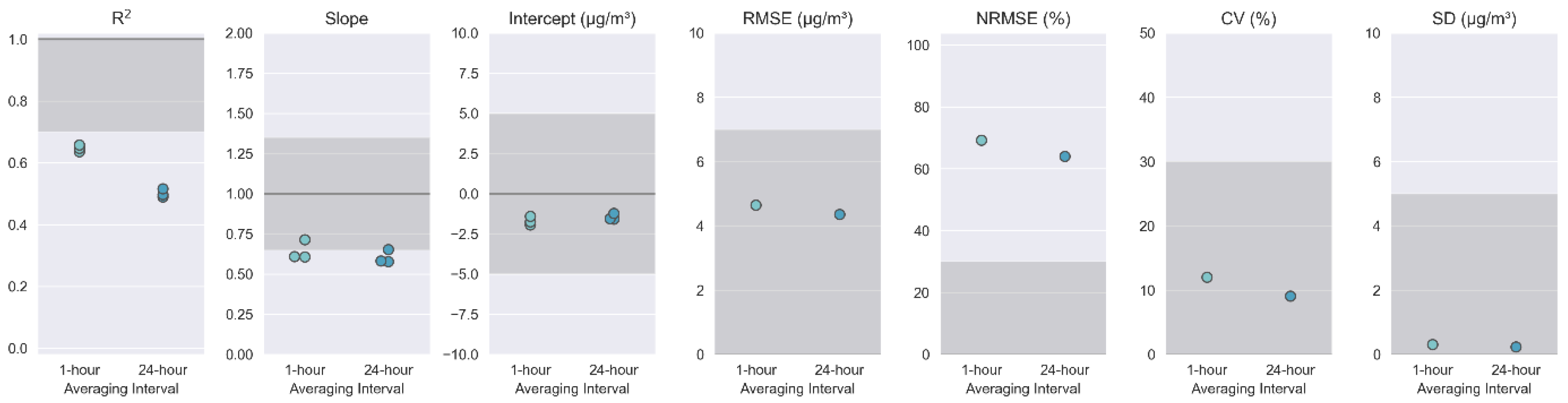
The SensorEvaluation.plot_metrics()method creates a plot that visualizes how the performance metrics for the sensor compares to the target values proposed in Sensor Targets Reports. This plot is a series of adjacent subplots each corresponding to a different metric. Ideal performance values are indicated by a dark gray line across the plot although RMSE, normalized RMSE (NRMSE), CV, and SD would ideally all be zero making this line difficult to see. Target ranges are indicated by gray shaded regions. The calculated metric for each sensor (R2, slope, intercept) or the ensemble of sensors (RMSE, NRMSE, CV, SD) are shown as small circles. Metrics are calculated for each of the time averaging intervals specified in the Parameter object. These graphs assist users in quickly determining which target values are met, how close the sensors are to meeting the missed targets, if there is variation among the batch of sensors tested, and if time averaging interval affects the sensor’s ability to meet the targets.
The SensorEvaluation.plot_met_dist() method plots the relative frequency of meteorological measurements recorded during the testing period in a bar graph. Temperature (T) and relative humidity (RH) data reflects measurements by the independent meteorological instrument at the monitoring site. The time averaging interval is displayed in the figure header. These graphs assist users in determining whether the test conditions are similar to conditions in the intended deployment location. If deployment conditions are likely to be significantly different, further testing is advised before deployment.
The SensorEvaluation.plot_met_influence() method creates plots to visualize the influence of T or RH on sensor measurements. Sensor concentration measurements are normalized by (i.e., divided by) the reference concentration measurements and then plotted on the y-axis. T and RH, as measured by the independent meteorological instrument at the monitoring site, are plotted on the x-axis. These graphs assist users in determining whether T and RH influence the performance of the sensor. For instance, if the RH graph shows an upward trend, it would indicate that the sensor concentration measurements are higher during high humidity conditions. Thus, users may wish to include a RH component when developing a correction equation for the sensor measurements.
The SensorEvaluation.plot_wind_influence() method is an optional plot to visualize the influence of wind speed and direction on sensor measurements. For wind speed, sensor concentration measurements are shown as the concentration difference between the sensor and reference monitor and plotted on the y-axis. For wind direction, concentration measurements reported by the sensor are shown as the absolute value of the concentration difference between the sensor and reference monitor and plotted on the y-axis. These graphs assist users in determining whether wind speed and wind direction influence the performance of the sensor.
In addition to plots, the SensorEvaluation object can print descriptive summaries to the console. The SensorEvaluation.print_eval_metrics() method prints a summary of the performance metrics along with the average value and the range (min to max) for that metric for each of the collocated sensors. The SensorEvaluation.print_eval_conditions() method prints a summary of the mean (min to max) pollutant concentration as reported by both the sensor and reference monitor and meteorological conditions (T and RH) experienced during the testing period. These summaries are displayed for each of the time averaging intervals specified in the Parameter object.
2.4.4. Performance Report Object
The PerformanceReport object takes the output from the SensorEvaluation object to create a testing report utilizing the Sensor Targets Report reporting template. Information about the testing organization and testing site, specified in the initial setup script, are included at the top of the first page of the testing report. Details about the sensor and FRM/FEM reference instrumentation will be populated into the report from the information obtained in the sensor and reference data ingestion module but can also be adjusted or added manually after the report is created.
Several plots generated via the SensorEvaluation object are displayed on the first page including the time series plots, one scatterplot, performance metrics and target value plots, the T and RH frequency plots describing test conditions, and plots describing meteorological influences on the sensor data. One goal of the reporting template is to provide as much at-a-glance information as possible on this first page.
The second page of the report is populated with a tabular summary of the performance metrics including R2, slope, and intercept for each of the collocated sensors. The tabular summary makes it easier to compare the metrics with the performance targets. Scatterplots for each collocated sensor are displayed on this page or the subsequent page depending on space. Multiple scatterplots are presented here to allow users to visually compare performance among the cadre of sensors.
The subsequent pages of the reporting template are designed to document supplemental information, and testers can begin populating this material after the report is generated. In accordance with the requested information in the Sensor Targets Reports, a large table of supplemental information is printed. Testers can use the check boxes to note if information is available and can manually enter details or URLs as available. If testers require more space or choose to provide more information, additional information can be added to the end of the report.
3. Results
As a case study, the sensortoolkit Python code library was used to evaluate the performance of PurpleAir sensors deployed in triplicate in the Durango Complex in Phoenix, Arizona during May 2019. Device or algorithm changes made by the manufacturer since this test may have changed performance. Figure 3 shows the testing meta data dictionaries for organization information and testing location details. This information is used to populate testing reports.
Sensor data were read from three local csv files (assigned the unique serial identifiers PA01, PA03, PA05) and we focused on the cf=atm estimates (PM2.5 and PM10) from channel A. The AirSensor.sensor_setup() method describes the contents of those files, indicates the SDFS parameters associated with each column, describes the timestamp format, specifies the time zone, and assigns each sensor a unique identifier derived from the serial number. A flow chart of this process is shown in Figure 2. Users who wish to analyze files from sensors of the same make, model, and firmware version for subsequent evaluations may use an existing setup.json file in the sensor_setup() module. Since the data formatting will be similar, this saves time by reducing the amount of manual entry required to instruct the setup routine how to convert the sensor-specific data format into the SDFS data structure. For this report, we ran the reference_setup() module and reference data was ingested locally. The SI file “case_study_Base_Testing_Report_PM25_Test_Testing_241120.pptx” contain pages 1-4 of the report generated that evaluates PM2.5 sensor performance.
On the first page of the report, the time series (Figure 4) graph shows the PM2.5 pollutant concentrations reported by the reference FEM instrument and the three collocated sensors. The top graph shows 1-hour averages, and the bottom graph shows 24-hour averages. From these graphs, users can see that the sensors display the same trends as the reference instrument. Sensors usually under-report concentrations throughout the concentration range experienced in this test.
Scatterplots for individual sensors are included in the report and shown in Figure 5. These graphs indicate that the 1-hour averaged PM2.5 sensor concentrations have a fairly strong linear relationship with the reference FEM instrument (R2 = 0.64-0.66) and all sensors have similar error (RMSE = 4.42-4.94 µg/m3). Sensors generally under-report concentrations in this concentration range. The time synced data points are colored based on reference RH which is low in this geographical area (predominantly <50%, see Figure 7). In Figure 5, a prominent two prong relationship is observable with the lower “arm” showing that the sensors frequently under-report the ambient concentration. This “arm” correlates with seasonal dust events. The dust events include both fine and coarse particles which elevates PM2.5 and PM10 concentrations. Further discussion of the sensor’s PM10 performance will be presented later in this section (Figure 10).
The first page of the report includes the performance metrics and target values/ranges graph. Potential users can quickly determine that these sensors meet the performance targets for the intercept (a portion of bias measurement), error (RMSE), and precision (CV and SD). These sensors nearly meet the target for slope (another bias measurement) which may be addressed using a correction equation. Although the NRSME error target is not met, this metric can be influenced by the concentration range experienced during the test so it can be deprioritized as the Sensor Targets Report suggests it is a more important metric as concentrations become higher (e.g., wildfire smoke conditions). The sensors do not meet the linearity (R2) target with 24-hour averaged data but are closer to the target at 1-hour averages (R2=0.64-0.66). Linearity improvements may be possible with more complex data processing algorithms to handle periods impacted by dust.
Figure 6.
PM2.5 performance metrics (colored dots) and target value/range (darker grey shading) showing how the performance of these sensors compares to the targets at both 1-hour and 24-hour averages.
Figure 6.
PM2.5 performance metrics (colored dots) and target value/range (darker grey shading) showing how the performance of these sensors compares to the targets at both 1-hour and 24-hour averages.
At the bottom of the first page are two pairs of graphs (Figure 7 and Figure 8) that investigate T and RH. Figure 7 summarizes the 1-hour averaged T and RH, as measured by the reference station’s meteorological instruments during the collocation period. Potential users should note that additional testing may be needed if these sensors will be used in colder climates (T < 24°C or ~70°F) or more humid climates (RH > 75%). This test cannot provide insight as to performance or robustness of the sensors under those conditions. Figure 8 shows how the normalized (sensor/reference) PM2.5 concentrations change as a function of T and RH. In this case, there is little to no observable trend suggesting RH may not largely impact sensor performance.
Figure 7.
Relative probability of temperature (left) and relative humidity (right) recorded during the testing period are displayed as histograms. Measurements are grouped into 15 bins, and the frequency measurements within bin is normalized by the total number of measurements.
Figure 7.
Relative probability of temperature (left) and relative humidity (right) recorded during the testing period are displayed as histograms. Measurements are grouped into 15 bins, and the frequency measurements within bin is normalized by the total number of measurements.
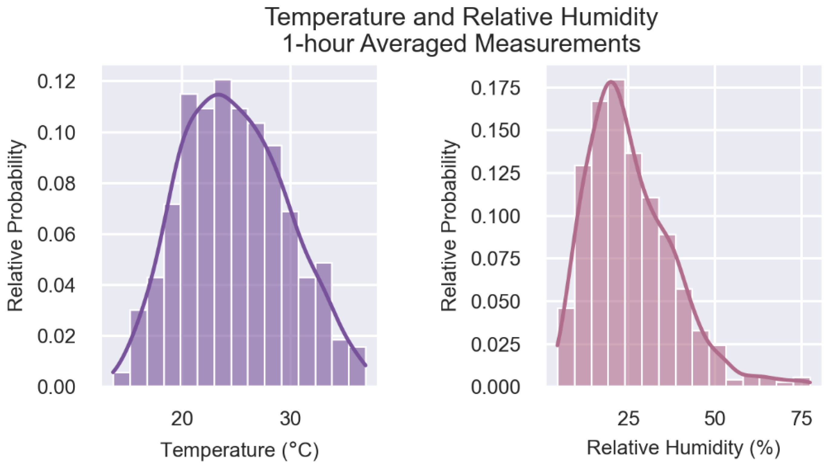
Figure 8.
1-hour sensor measurements divided by each hourly reference measurements (i.e., Normalized PM2.5) are shown for temperature (left) and relative humidity (right). Scatter plots for each sensor are displayed as well as a gray 1:1 line that indicates ideal agreement between the sensor and reference measurements over the range of metrological conditions.
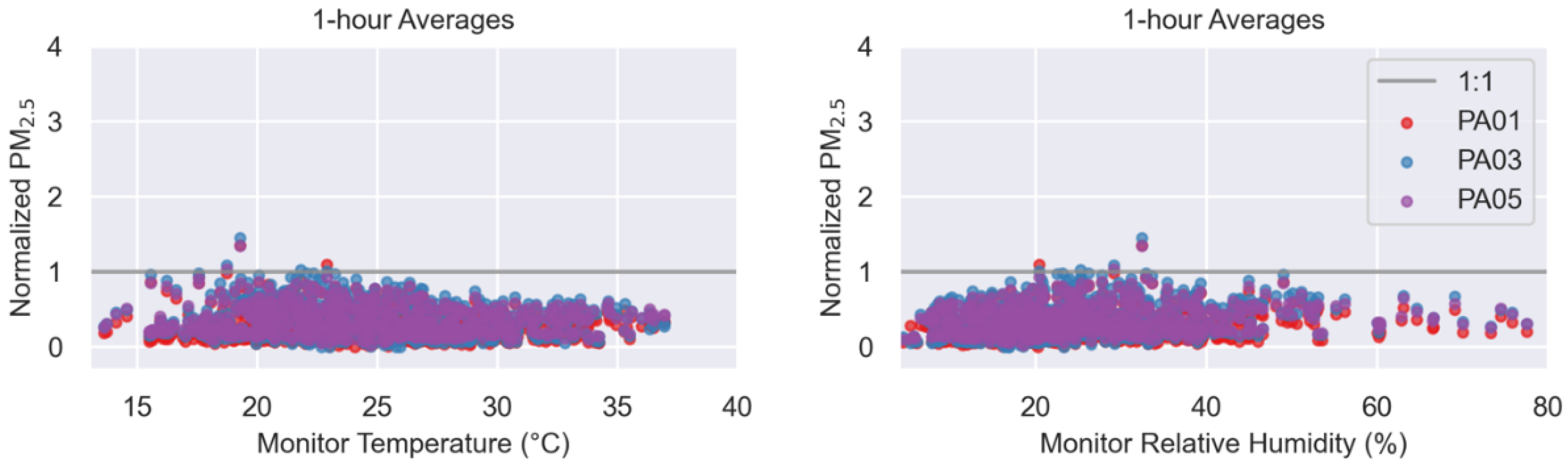
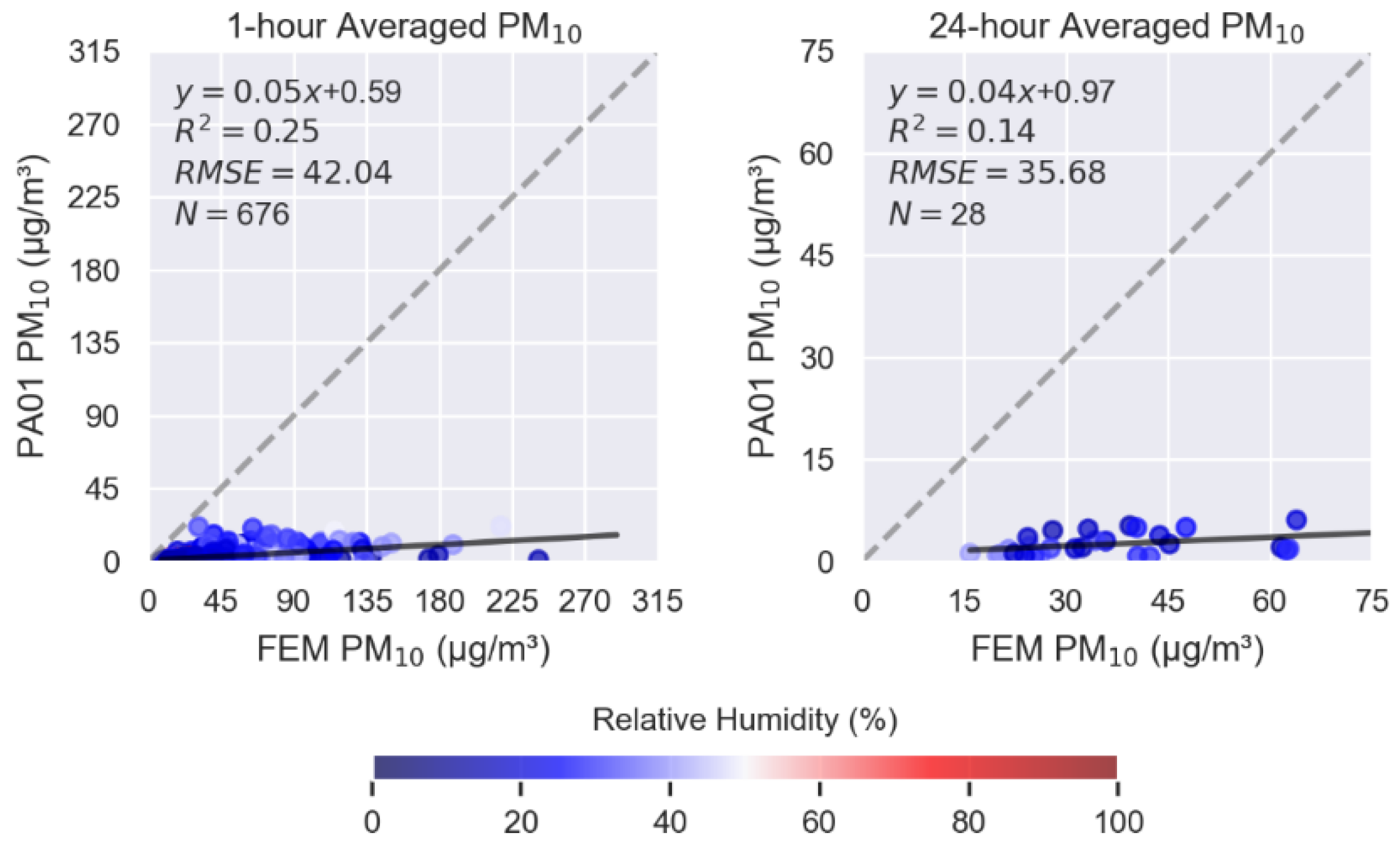
Figure 9 shows similar 1-hour averaged scatterplots with the same sensor and reference data source but for PM10. The slope indicates that the sensors significantly under-report PM10 concentrations. With weak linearity and high error, the sensors do not perform well in measuring PM10 and would not be a good choice for projects aimed at understanding dust exposure and sources.
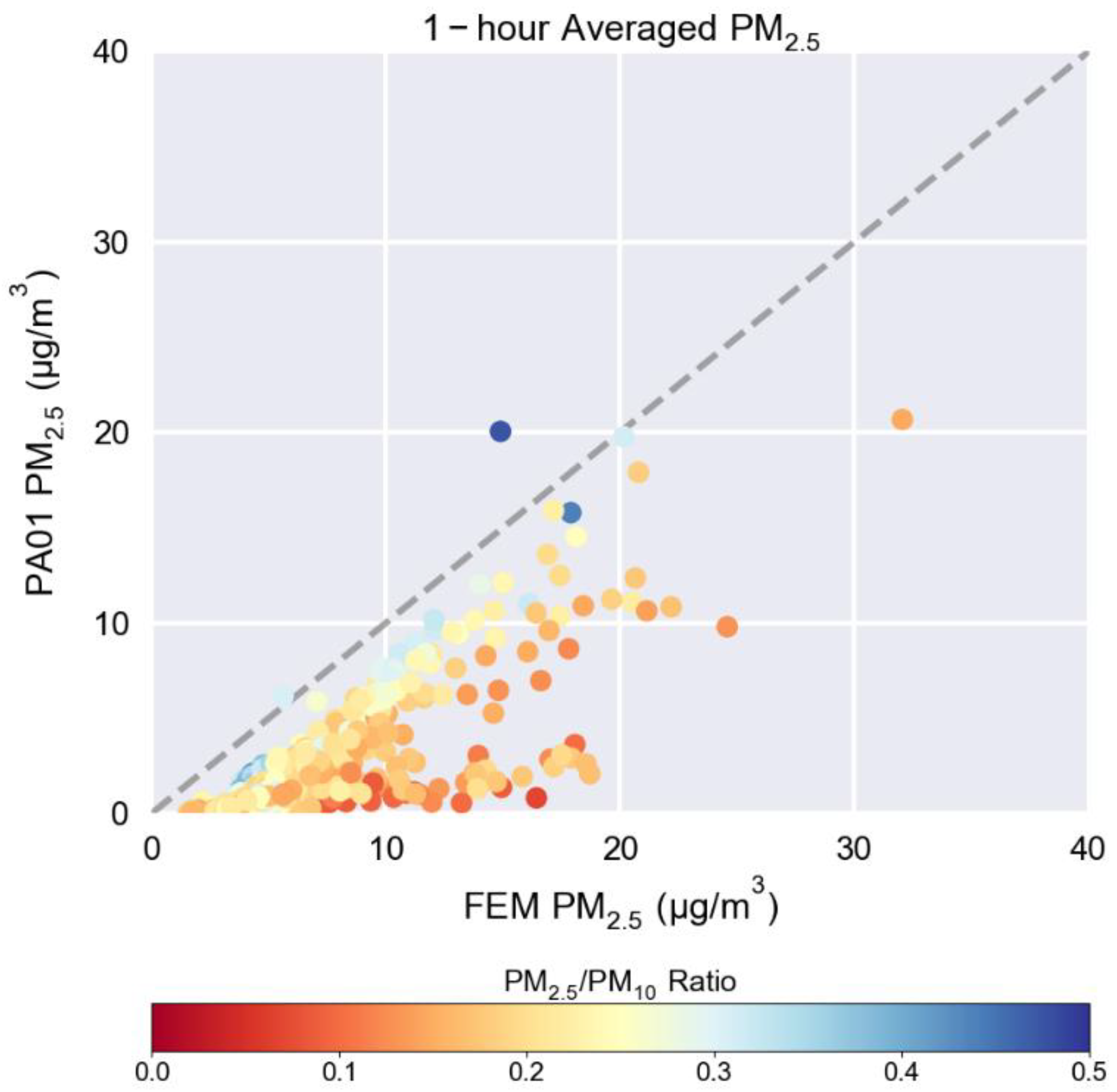
The PA01 sensor plot from Figure 5 is shown again in Figure 10 but this time the dots are colored by the PM2.5/PM10 ratio as measured by a collocated reference instrument. This is an example of an exploratory plot that testers might find useful in further explaining some of the observations made during testing. Figure 10 was not created within sensortoolkit but is an example of how further analysis is made easier by starting with the reformatted data files and the calculated ratio created by the tool. The PM2.5/PM10 ratio can be used to better understand if there is variation in the particle size distribution. The “arm” that shows significant under-reporting has a lower PM2.5/PM10 ratio when compared to points that lie closer to the 1:1 line, indicating that higher concentrations of larger particles occur during this time period consistent with the observed dust events. As hypothesized previously, the sensor’s PM2.5 performance may be enhanced if shifts in the particle size distribution could be identified using only the sensor’s measurements.
Figure 10.
1-hour averaged PM2.5 concentration scatterplot for 1 of the collocated sensors showing the 1:1 line (gray dotted line) and plot markers colored by PM2.5/PM10 ratio.
Figure 10.
1-hour averaged PM2.5 concentration scatterplot for 1 of the collocated sensors showing the 1:1 line (gray dotted line) and plot markers colored by PM2.5/PM10 ratio.
4. Discussion
The U.S. EPA developed the sensortoolkit as a free, open-source tool to assist testers in generating a summary of results from sensor performance evaluations based on the Sensor Targets Reports. This manuscript introduces the python code library and highlights:
- User needs that guided the creation of this tool,
- Data ingestion methodology to handle variation in data format,
- Standardization in performance metric calculations,
- Data visualizations,
- Motivations for the reporting template design, and
- A demonstration of the tool via a case study of sensor deployed in Phoenix, AZ.
We hope that consistency in reporting testing results will help standardize sensor performance evaluation approaches and encourage innovation and improvements in sensor technologies. Additionally, we hope that consumers can make more informed decisions when purchasing sensors by allowing them to compare the standard list of performance metrics to find options that are most appropriate for their application of interest.
Supplementary Materials
The following supporting information can be downloaded at the website of this paper posted on Preprints.org. Table S1: sensortoolkit Data Formatting Scheme Parameters, PurpleAir PM2.5 sensor performance testing report from Phoenix, AZ: Supplemental1_CaseStudy_PM25_Test_Report.pdf, and PurpleAir PM10 sensor performance testing report from Phoenix, AZ: Supplemental2_CaseStudy_PM10_Test_Report.pdf.
Author Contributions
Conceptualization, A.L.C. and S.G.F.; methodology, S.G.F.; software, S.G.F and M.K.; validation, K.K.B. and M.K.; formal analysis, S.G.F.; investigation, A.L.C. and S.G.F.; resources, A.L.C.; data curation, K.K.B. and S.G.F.; writing—original draft preparation, S.G.F, M.K., and A.L.C..; writing—review and editing, A.L.C., K.K.B., M.K., and S.F.G.; visualization, S.F.G. and M.K.; supervision, A.L.C. and K.K.B.; project administration, A.L.C.; funding acquisition, A.L.C.. All authors have read and agreed to the published version of the manuscript.
Funding
This work was funded internally by U.S. EPA by the Air, Climate, and Energy National Research Program. This research received no external funding.
Data Availability Statement
After publication, the U.S. EPA will make the data underlying this manuscript available at https://doi.org/10.23719/1531904. The data was collected as part of a larger research effort called Phoenix-as-a-Testbed for Air Quality sensors (P-TAQS). The larger dataset is available at https://doi.org/10.5281/zenodo.15174476.
Acknowledgments
Special thanks to Maricopa County Air Quality Department for site access, reference data, and field study support. Thank you to the current and former Jacobs Technology staff (Parik Deshmukh, Cortina Johnson, Brittany Thomas) who installed, monitored, and compiled data from the Phoenix monitoring site. We wish to thank Sue Kimbrough (retired U.S. EPA), Ian VonWald (former ORISE Postdoc at U.S. EPA) and Carry Croghan (U.S. EPA) for their work to compile, quality assure, and document the case study dataset. We appreciate the support of technical reviewers including Terry Brown (U.S. EPA), James Hook (U.S. EPA), Ashley Collier-Oxandale (formerly with South Coast Air Quality Management District), and Ken Docherty (Jacobs Technology) who initially reviewed the sensortoolkit code, Terry Brown (U.S. EPA) and Farnaz Nojavan Asghari (U.S. EPA) who reviewed an update to sensortoolkit after the release of additional Sensor Targets Reports, Amanda Kaufman (U.S. EPA) and Jack Balint-Kurti (summer intern from Duke University) who gave suggestions for documentation edits, and Rachelle Duvall (U.S. EPA) and Justin Bousquin (U.S. EPA) who thoughtfully reviewed this manuscript.
Conflicts of Interest
The authors declare no conflicts of interest.
Abbreviations
The following abbreviations are used in this manuscript:
| API | Application Programming Interface |
| AQMD | Air Quality Management District |
| AQS | Air Quality System |
| AZ | Arizona |
| CO | Carbon Monoxide |
| CV | Coefficient of Variation |
| FEM | Federal Equivalent Method |
| FRM | Federal Reference Method |
| GMT | Greenwich Mean Time |
| ID | Identification Number |
| IDE | Integrated Development Dnvironment |
| MDPI | Multidisciplinary Digital Publishing Institute |
| N | Number of Data Points |
| NO2 | Nitrogen Dioxide |
| NRMSE | Normalized Root Mean Square Error |
| O3 | Ozone |
| ORAU | Oak Ridge Associated Universities |
| ORISE | Oak Ridge Institute for Science and Education |
| P-TAQS | Phoenix-as-a-Testbed for Air Quality Sensors |
| PM | Particulate Matter |
| PM2.5 | Fine Particulate Matter |
| PMc or PM10-2.5 | Coarse Particulate Matter |
| PM10 | Particles with diameters that are generally less than 10 micrometers |
| PyPI | Python Packaging Index |
| R2 | Coefficient of Determination |
| RH | Relative Humidity |
| RMSE | Root Mean Square Error |
| SD | Standard Deviation |
| SDFS | Sensortoolkit Data Formatting Scheme |
| SO2 | Sulfur Dioxide |
| T | Temperature |
| U.S. EPA | United States Environmental Protection Agency |
| URL | Uniform Resource Locator |
| UTC | Coordinated Universal Time |
References
- Kelly, K.E., et al. Community-Based Measurements Reveal Unseen Differences during Air Pollution Episodes. Environmental Science & Technology 2021, 55, 120-128. [CrossRef]
- Mohammed, W., et al. Air Quality Measurements in Kitchener, Ontario, Canada Using Multisensor Mini Monitoring Stations. Atmosphere 2022, 13, 83. [CrossRef]
- Madhwal, S., et al. Evaluation of PM2.5 spatio-temporal variability and hotspot formation using low-cost sensors across urban-rural landscape in lucknow, India. Atmospheric Environment 2024, 319, 120302. [CrossRef]
- Snyder, E.G., et al. The Changing Paradigm of Air Pollution Monitoring. Environmental Science & Technology 2013, 47, 11369-11377. [CrossRef]
- Smoak, R., Clements A., Duvall, R. Best Practices for Starting an Air Sensor Loan Program. 2022. Available online: https://cfpub.epa.gov/si/si_public_record_report.cfm?Lab=CEMM&dirEntryId=355832 (accessed on 24 July 2025).
- D’eon, J.C., et al. Project-Based Learning Experience That Uses Portable Air Sensors to Characterize Indoor and Outdoor Air Quality. Journal of Chemical Education 2021, 98, 445-453. [CrossRef]
- Griswold, W., Patel, M., and Gnanadass, E. One Person Cannot Change It; It's Going to Take a Community: Addressing Inequity through Community Environmental Education. Adult Learning 2024, 35, 23-33. [CrossRef]
- Collier-Oxandale, A., et al. Towards the Development of a Sensor Educational Toolkit to Support Community and Citizen Science. Sensors 2022, 22. [CrossRef]
- Clements, A.L., et al. Low-Cost Air Quality Monitoring Tools: From Research to Practice (A Workshop Summary). Sensors 2017, 17. [CrossRef]
- Wong, M., et al. Combining Community Engagement and Scientific Approaches in Next-Generation Monitor Siting: The Case of the Imperial County Community Air Network. International Journal of Environmental Research and Public Health 2018, 15. [CrossRef]
- Farrar, E., et al. Campus–Community Partnership to Characterize Air Pollution in a Neighborhood Impacted by Major Transportation Infrastructure. ACS ES&T Air 2024. [CrossRef]
- Barkjohn, K.K., et al. Air Quality Sensor Experts Convene: Current Quality Assurance Considerations for Credible Data. ACS ES&T Air 2024. [CrossRef]
- Feenstra, B., et al. Performance evaluation of twelve low-cost PM2.5 sensors at an ambient air monitoring site. Atmospheric Environment 2019, 216, 116946. [CrossRef]
- Williams, R., et al. Deliberating performance targets workshop: Potential paths for emerging PM2.5 and O3 air sensor progress. Atmospheric Environment: X 2019, 2, 100031. [CrossRef]
- Duvall, R.M., et al. Deliberating Performance Targets: Follow-on workshop discussing PM10, NO2, CO, and SO2 air sensor targets. Atmospheric Environment 2020, 118099. [CrossRef]
- Kaur, K. and Kelly, K.E. Performance evaluation of the Alphasense OPC-N3 and Plantower PMS5003 sensor in measuring dust events in the Salt Lake Valley, Utah. Atmospheric Measurement Techniques 2023, 16, 2455-2470. [CrossRef]
- Ouimette, J., et al. Fundamentals of low-cost aerosol sensor design and operation. Aerosol Science and Technology 2023, 1-44. [CrossRef]
- Giordano, M.R., et al. From low-cost sensors to high-quality data: A summary of challenges and best practices for effectively calibrating low-cost particulate matter mass sensors. Journal of Aerosol Science 2021, 158. [CrossRef]
- Hagan, D.H. and Kroll, J.H. Assessing the accuracy of low-cost optical particle sensors using a physics-based approach. Atmospheric Measurement Techniques 2020, 13, 6343-6355. [CrossRef]
- Wei, P., et al. Impact Analysis of Temperature and Humidity Conditions on Electrochemical Sensor Response in Ambient Air Quality Monitoring. Sensors 2018, 18, 59. [CrossRef]
- Duvall, R., et al. Performance Testing Protocols, Metrics, and Target Values for Fine Particulate Matter Air Sensors: Use in ambient, outdoor, fixed site, non-regulatory supplemental and informational monitoring applications. U.S. Environmental Protection Agency 2021.
- Duvall, R.M., et al. Performance Testing Protocols, Metrics, and Target Values for Ozone Air Sensors: Use in ambient, outdoor, fixed site, non-regulatory supplemental and informational monitoring applications. U.S. Environmental Protection Agency 2021.
- Duvall, R., et al. NO2, CO, and SO2 Supplement to the 2021 Report on Performance Testing Protocols, Metrics, and Target Values for Ozone Air Sensors. U.S. Environmental Protection Agency 2024.
- Levy Zamora, M., et al. Evaluating the Performance of Using Low-Cost Sensors to Calibrate for Cross-Sensitivities in a Multipollutant Network. ACS ES&T Engineering 2022, 2, 780-793. [CrossRef]
- Duvall, R., et al. PM10 Supplement to the 2021 Report on Performance Testing Protocols, Metrics, and Target Values for Fine Particulate Matter Air Sensors, U.S. Environmental Protection Agency 2023.
- Collier-Oxandale, A., et al. AirSensor v1.0: Enhancements to the open-source R package to enable deep understanding of the long-term performance and reliability of PurpleAir sensors. Environmental Modelling & Software 2022, 148, 105256. [CrossRef]
- Feenstra, B., et al. The AirSensor open-source R-package and DataViewer web application for interpreting community data collected by low-cost sensor networks. Environmental Modelling & Software 2020, 134, 104832. [CrossRef]
- Carslaw, D.C. and Ropkins K. openair — An R package for air quality data analysis. Environmental Modelling & Software 2012, 27-28, 52-61. [CrossRef]
- Anaconda, Anaconda Software Distribution. 2016.
Figure 1.
Schematic showing the sensortoolkit objects and general flow of information from data files to creation of the sensor performance report.
Figure 1.
Schematic showing the sensortoolkit objects and general flow of information from data files to creation of the sensor performance report.
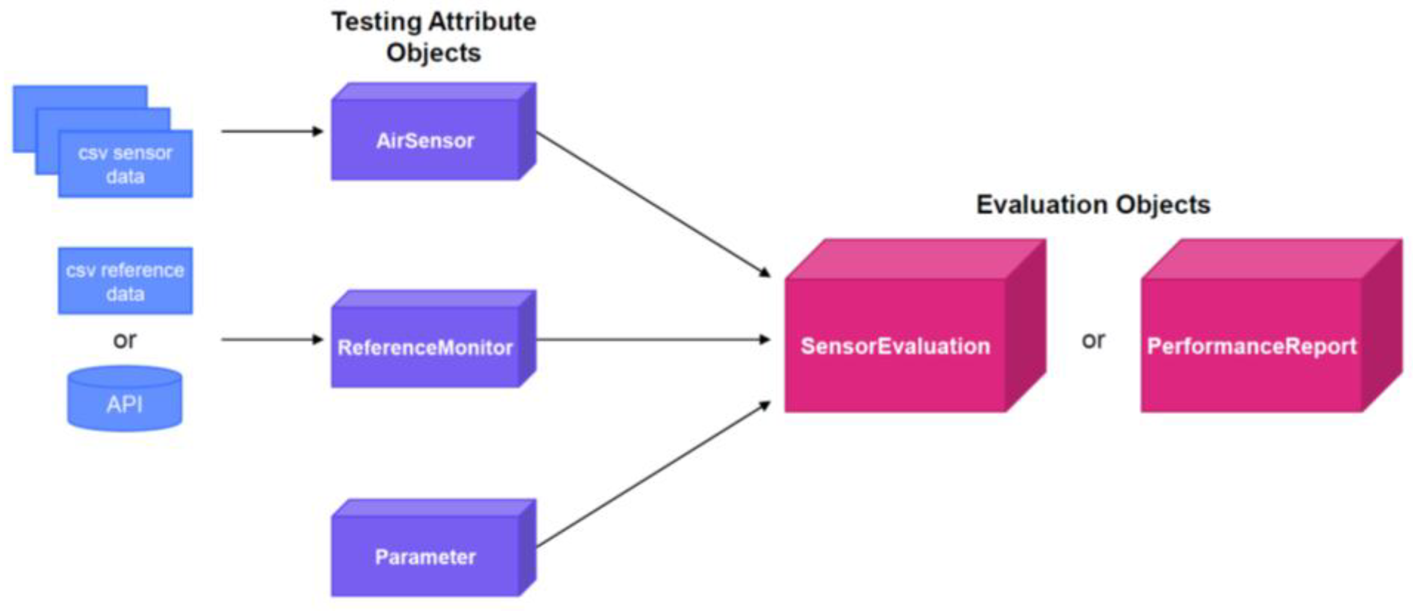
Figure 2.
Flowchart of the choices and steps involved in the sensor_setup() module.
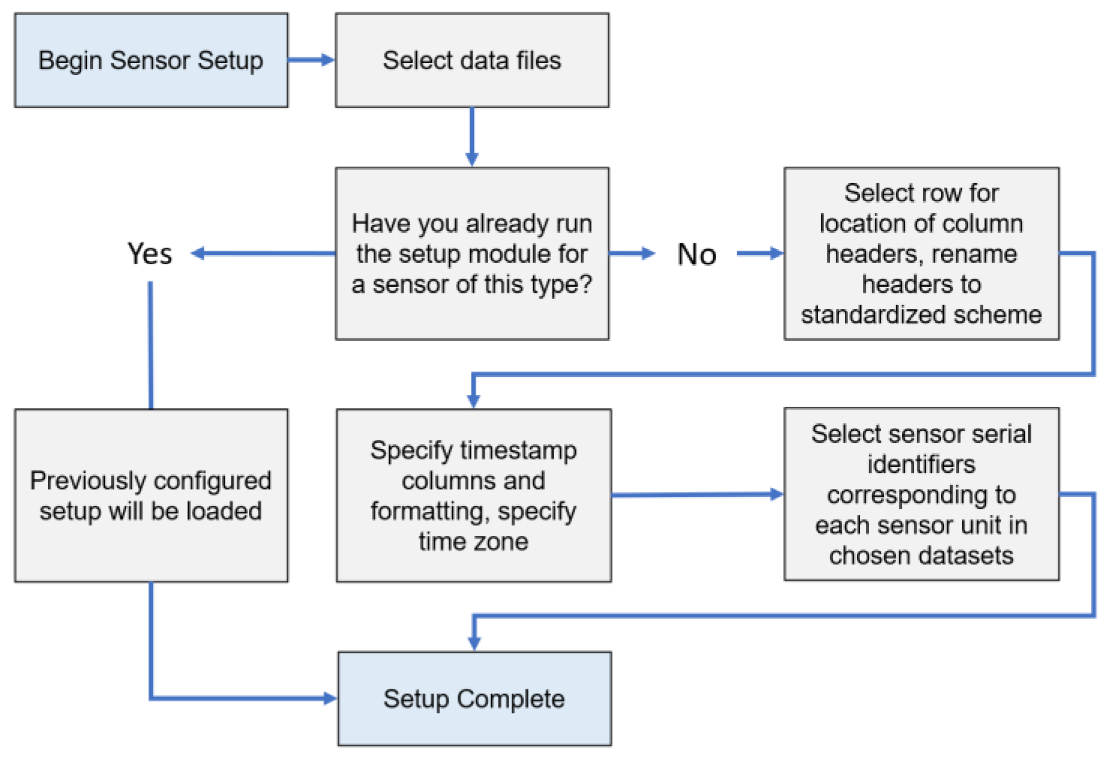
Figure 3.
Meta data initially provided to sensortoolkit to be displayed on the report generated.
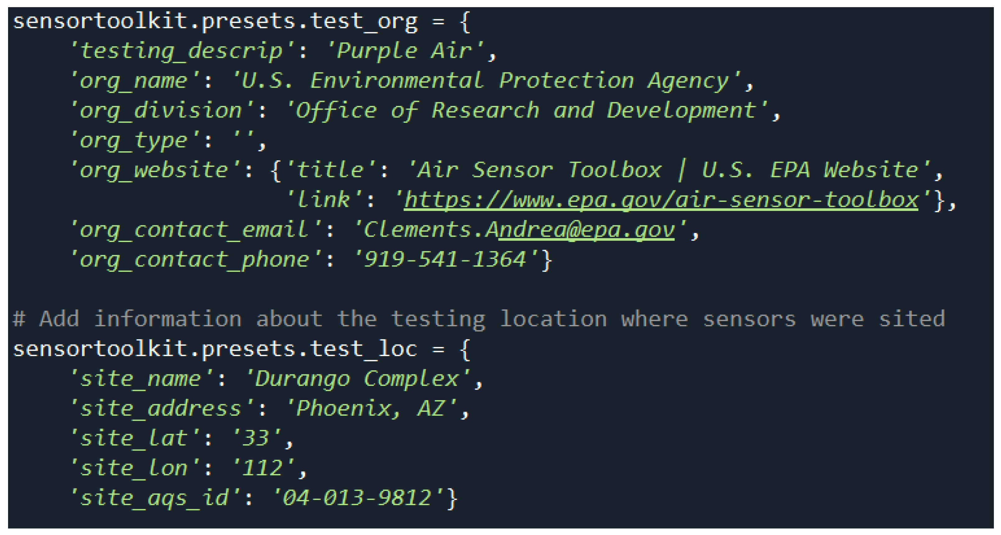
Figure 4.
Time Series Plots (1-hour top, 24-hour bottom) on Page 1 of the reporting template. Black lines represent the reference instrument, and colored lines represent the sensors.
Figure 4.
Time Series Plots (1-hour top, 24-hour bottom) on Page 1 of the reporting template. Black lines represent the reference instrument, and colored lines represent the sensors.
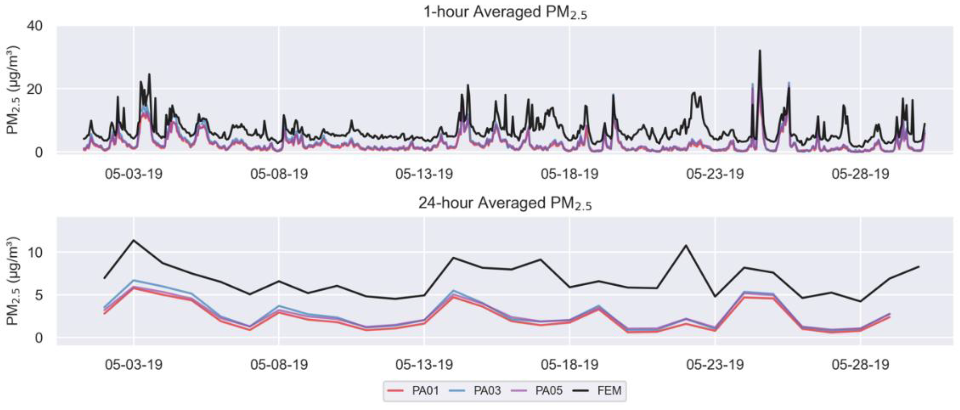
Figure 5.
1-hour averaged PM2.5 concentration scatterplots for each of the three collocated sensors showing the linear regression (black line), 1:1 line (gray dotted line), and summary statistics (upper left of each graph). Dots are colored by relative humidity.
Figure 5.
1-hour averaged PM2.5 concentration scatterplots for each of the three collocated sensors showing the linear regression (black line), 1:1 line (gray dotted line), and summary statistics (upper left of each graph). Dots are colored by relative humidity.
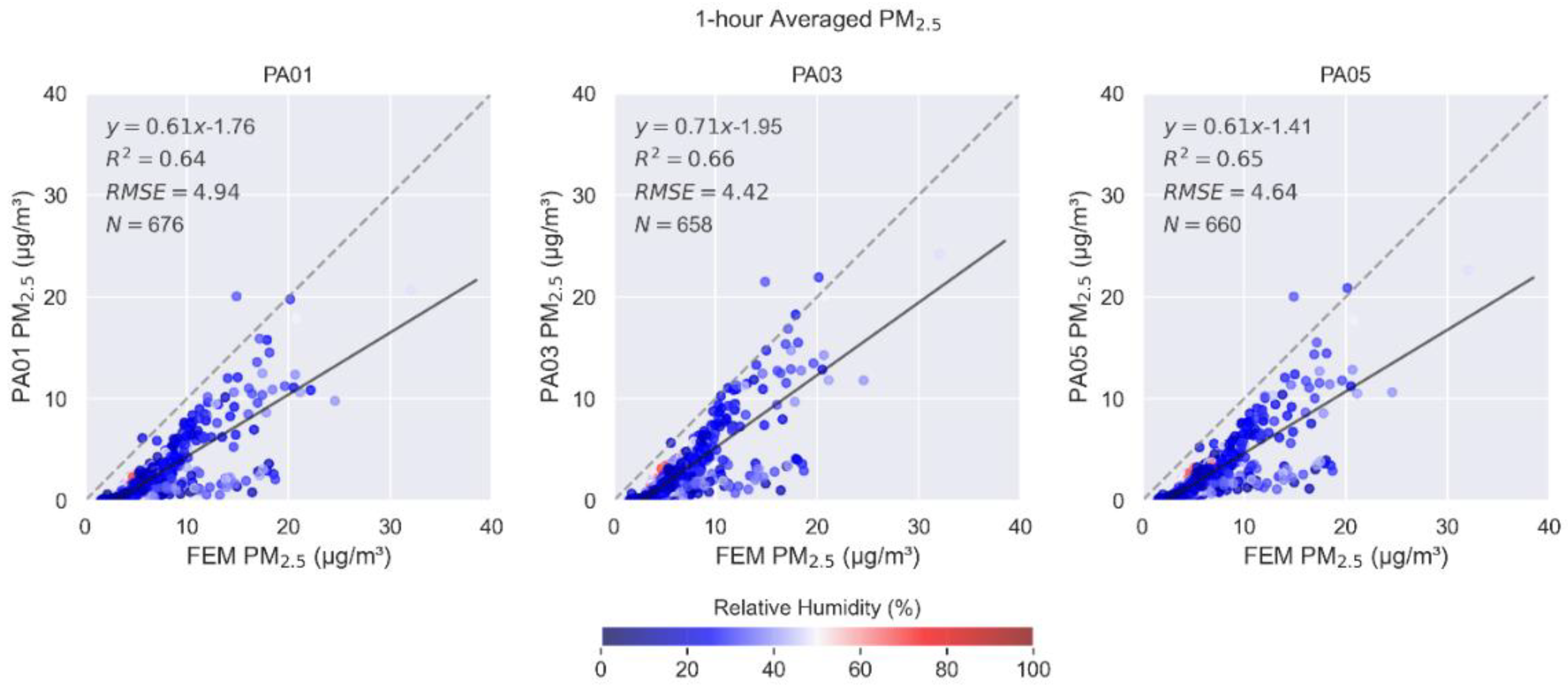
Figure 9.
1-hour averaged PM10 concentration scatterplots for one of the collocated sensors.
Disclaimer/Publisher’s Note: The statements, opinions and data contained in all publications are solely those of the individual author(s) and contributor(s) and not of MDPI and/or the editor(s). MDPI and/or the editor(s) disclaim responsibility for any injury to people or property resulting from any ideas, methods, instructions or products referred to in the content. |
© 2025 by the authors. Licensee MDPI, Basel, Switzerland. This article is an open access article distributed under the terms and conditions of the Creative Commons Attribution (CC BY) license (http://creativecommons.org/licenses/by/4.0/).
Copyright: This open access article is published under a Creative Commons CC BY 4.0 license, which permit the free download, distribution, and reuse, provided that the author and preprint are cited in any reuse.


