

Submitted:
20 October 2026
Posted:
21 October 2026
You are already at the latest version
Abstract
Starting from the representation of De Moivre’s matrix formula combined with the Kronecker product, we derive a 4 × 4 matrix Mθ that encodes algebraic properties with topological implications in four dimensions. This matrix describes trans- formations associated with symmetry and antisymmetry, encompassing distortion, dilation/contraction, and combined shear in a four-dimensional framework. We de- compose Mθ into its symmetric (S) and antisymmetric (Aanti ) components, a result that characterizes key features of the Alpha Group, including the formation of a tan- gent plane at infinity and its corresponding topological and geometric consequences. To investigate the system’s dynamics, we perform Monte Carlo simulations for varying values of the parameter θ, revealing attractor behavior and geometric transitions between Euclidean and hyperbolic regimes in projected three-dimensional trajectories.
Keywords:
abstract algebra
; group theory
; abstract geometry
; Lie algebra
; four-dimensional space
MSC: Primary: 20N05; 51H10; 57R18; Secondary: 37C55; 37N20; 53Z05
1. Introduction
Understanding geometric and topological objects in dimensions higher than three remains a central challenge in mathematical physics. Depending on the topological spaces involved, especially those close to tangent surfaces that approach infinity, great difficulty arises, since human perception is not naturally equipped to conceptualize topological arrangement with multiple degrees of freedom and complex spatial symmetries.
In the development of mathematical thinking and projective notions, Poncelet [37] observed that the general equation for a conic section may be expressed as:
When examining the special case where and , the formula becomes a sum of squares:
which yields the trivial solution , an isolated point. Alternatively, the expression determines imaginary lines, intersecting the -plane only at the origin. In this context, Poncelet aimed to characterize the geometric properties of imaginary elements, proposing that projections could occur even without intersection with the real plane, thus producing imaginary elements in geometry.
Chaves and Grimberg [7] discussed the work of 19th-century mathematicians such as Poncelet, Chasles, and others, who sought to give geometric meaning to expressions such as “infinite points” and “imaginary elements,” in accordance with Poncelet’s principles from 1820 [36], 1864 [38], and 1866 [39], often referred to as the principle of permanence or continuity of mathematical relations. While this idea parallels Carnot’s, Poncelet extended it by proposing the existence of points at infinity, a concept previously hinted at by Kepler and Descartes. Consequently, it became acceptable to say that two lines always intersect: either at a real point or, in the case of parallel lines, at a point at infinity, which Poncelet called the point at infinity.
Poncelet argued that, to generalize geometric reasoning, both imaginary and ideal points must be admitted into synthetic geometry. Under this model, any circle and any straight line will always intersect. Chasles [6] and Loud [27] demonstrated that points at infinity could not physically exist on geometric figures, as they are impossible to construct. Nonetheless, they used the principle of continuity to define the concept of an imaginary point. Thus, Poncelet’s concept of continuity can be fruitfully extended to mathematical analysis within the realm of pure geometry.
As a result, Corrêa et al. [10,11] proposed the Alpha group theory, based on the notion of multiple types of infinities grounded in group theory and Cantor’s ideas [5]. In Cantor set theory, a hierarchy of infinities is established. While infinity is often treated as an indeterminate concept, under a geometric and topological perspective, it can be associated with specific types of structured infinity. Cantor distinguished between potential infinity and actual infinity. The Alpha group, particularly through the introduction of the imaginary number , relates to actual infinity, where geometric and topological configurations are preserved.
Actual (or complete) infinity refers to infinity as a finished, completed quantity. It is treated as a concrete object or entity, one that exists as a complete “whole”, like a set that already contains an infinite number of elements [4,26].
[10,11], starting from group theory, demonstrated that the interaction of two infinite planes forms the Alpha group. These planes are connected by a transformation of the division operation, creating a third element with a morphism that preserves the algebraic configuration of both. This construction yields a topological and geometric representation of infinity.
The hypercomplex quaternion defined in the Alpha group consists of four components: a real term , a complex term , a third term , and a fourth term , where and represent two distinct imaginary components. The division operation, formulated using two De Moivre arrays, results in a matrix involving tangent and cotangent relationships. This matrix varies topologically as the angle ranges from 0 to , inducing changes in the geometry. At , the topology corresponds to the Euclidean space, whereas at , which corresponds to the Alpha group framework. Geometrically, at the infinite plane , a natural extension arises, revealing a higher complexity where the local (Euclidean) space “opens up” to exhibit novel geometric behavior. Terminology and Mathematical Scope. The term Extended Alpha Group is retained as the historical and conceptual designation of the mathematical construction developed in this work. It identifies the research framework in which the associated matrix representations, algebraic relations, and Lie-algebraic structures are investigated. The use of this designation does not replace the formal specification of the underlying mathematical objects or the verification of their defining properties. Accordingly, the algebraic and geometric structures discussed below are characterized by their explicit definitions and demonstrated properties, while the term Extended Alpha Group is maintained as the established name of the overall construction.
A relevant characteristic of the Alpha group is its role as an asymptotic attractor, a concept that describes how systems evolve, often stabilizing into specific configurations or behaviors. In curved spaces, as studied in differential geometry, the tangent plane is a crucial tool for analyzing local curvature and its relationship to global topology. The transition from local Euclidean space to infinite configuration implies that the tangent plane is acquiring a new geometry, one that is both topologically and symmetrically regular and capable of describing the transition to infinity. This work adopts a topological-first perspective: the global structure of space is determined by compactification, while geometry emerges as a local manifestation of this topology. The Alpha structure can be interpreted as a group-like extension, generalizing classical group structures by incorporating an idempotent operator and a topological projection mechanism.
2. Theoretical Model
The imaginary number can capture properties associated with singularities, such as characterizing geometric symmetries through rotations induced by changes in the angle . These symmetry transformations can be invariant (conservative), as their topology may correspond to Euclidean topology locally and to the topology associated with the Alpha group globally. In the topology of the space defined by the Alpha group, the behavior varies according to the angle in the interval , which can be interpreted as a transition between local and global descriptions of space. At , the space is locally Euclidean, corresponding to a classical flat-space description. In contrast, at , the space becomes “infinite", approaching a global configuration, such as the formation of a tangent plane.
This transition can be interpreted as an example that reveals a connection with gauge-like structures [42,44,46,48]. Furthermore, the resulting matrix exhibits geometric properties associated with rotations and Lie algebra in four dimensions [18,20,45].
In this work, we aim to explore the properties that arise from switching between rotations in four-dimensional space and rotations in two-dimensional planes (2D), as represented by the matrix . We will present the symmetric and antisymmetric relationships of these rotations, as well as examine how combinations of shear and dilation change within a four-dimensional space (4D) in the context of the Alpha group. Additionally, within the context of the Alpha group, we conjecture a connection with gauge-like theory [18].
3. Matrix Development and Properties
3.1. Foundations
De Moivre’s theorem served as the foundation for Murnaghan’s 1944 introduction of the quaternion theory. A complex number x+yi can be represented as a 2×2 square matrix using the following transformation [31].The definition and algebraic development of this operation are presented in a companion work [15], which provides the broader framework for the matrix construction used here:
As a result, De Moivre’s theorem can be expressed as follows:
The operation involving two matrices based on De Moivre’s formula can be used to generate elements of the Alpha group, even though the quaternion in the Alpha group can be composed of two complex planes using the equation in matrix form (2), which can be composed by dividing two matrices of type (2). Equation (3) by Weyl [12,50] illustrates how the division strategy is constructed in a similar way to the Kronecker product. There might be several methods to describe this operation; however, the solution of Equation (3) naturally came from the relationship between the operators.
The matrix provides the basis for investigating the dynamics associated with complex-conjugate eigenvalues and the possible coupling of two Hopf bundles. The construction originates from the matrix representation of De Moivre’s formula for a classical complex number, while the division operation determines the configuration of and motivates the associated algebraic structure of the Extended Alpha Group. The derivation is developed from the matrix form of De Moivre’s theorem in Equation (2), following the approach discussed in [10,12,13,14]. The construction of the Extended Alpha Group matrix is based on the matrix representation of De Moivre’s formula and the Kronecker product. Within this framework, the division operation between two matrix representations of De Moivre’s formula is used to obtain the four-dimensional matrix . The relationship between these operations follows the construction described in the cited references and provides the algebraic starting point for the analysis developed in this work.
The matrix , with its terms on the main diagonal , concretely represents the algebra of the Alpha group. The diagonal elements anchor the essence of each "mode" of the system with its intrinsic properties (including imaginary aspects and the topological invariant ). This represents two simultaneous dynamics: one real (rotation) and the other imaginary (distortion or bifurcation). The matrix M() appears to be a non-Hermitian structure, with explicit dependence on the angular parameter , and can be seen to generate internal vector variations. In the formulation of the Alpha group algebra, which can be defined as the multiplication of an angular matrix A() by another phase/amplitude matrix B().
The Alpha group matrix can be interpreted as a framework that exhibits a coherent dynamic associated with the fibers of its complex eigenvalues. At certain critical points, especially for:
Regular discontinuities (smooth bifurcations or transitions), qualitative changes in the topology, and the formation of dominant complex oscillatory solutions occur, coherently organizing space. These points function as natural rhythms of coherent alignment of fibers in higher-dimensional space.
3.2. Topological and Projective Definition of the Imaginary Number
We define as an idempotent operator encoding asymptotic directions, a topological and projective construct that arises from the compactification of space in four dimensions. Unlike the classical imaginary unit i, which arises from the field of complex numbers and satisfies , the entity is not a conventional algebraic number; instead, it behaves as a directional operator associated with the boundary of a compactified manifold. In projective geometry, points at infinity serve to close the space, making parallel lines intersect and transforming open geometries into closed, homogeneous structures. Inspired by this principle, we introduce as a directional component representing the asymptotic behavior of space, the geometric "flow" as it approaches its ideal boundary.
The number is defined by its behavior under angular transformations, which naturally manifests in the quaternionic formulation.
and interacts non-commutatively with i, satisfying . It represents a kind of imaginary axis that encodes the transition between local (Euclidean) and global (compactified) configurations.
Geometrically, corresponds to a compactified radial direction, a vector field projected onto the boundary at infinity. Its projective nature allows it to be treated not just as a symbolic placeholder but as a carrier of structural information in higher-dimensional algebra. In this model, serves as an asymptotic marker, characterizing deformations, attractors, and transitions in the global topology of space.
Thus, functions as a bridge between classical coordinate-based geometry and a new asymptotic configuration geometric algebra, allowing the construction of the Alpha group and its associated transformations in . We define as an extended imaginary unit with hybrid topological-projective properties. Algebraically, it satisfies and , positioning it as a non-commutative and idempotent imaginary unit. Topologically, serves as a projector in the compacted directions in , representing a radial vector pointing to the ideal limit at infinity, consistent with Alexandroff compactification [30] and projective closure. This endows with dual functionality: it is simultaneously an algebraic generator and a topological operator, forming the backbone of the Alpha group framework. The operator behaves as a topological projector, identifying all points in that recede to infinity and collapsing the asymptotic boundary into a single ideal point. Under this action, is extended by this point and, by the Alexandroff compactification [22,30,47], suggests a compactification compatible with a structure homeomorphic to . Accordingly, simultaneously performs the topological closure and the global projection , establishing the compact configuration required for the geometric and dynamical analysis developed in this work. The properties described above can be summarized in the following formal statement. Proposition (Compactification Induced by ). Let be the Alpha group matrix. In the limit , the action of induces a topological compactification of , which induces a compactification consistent with a structure homeomorphic to . Interpretation. As , the divergence of the trigonometric terms activates the asymptotic component of the transformation. The operator , acting as an idempotent projector, identifies directions tending to infinity, producing a compactified topological configuration.
3.3. Verification of Quaternion Structure
To justify the term hypercomplex quaternion, we demonstrate that the proposed framework satisfies the fundamental properties.
3.3.1. Multiplication Rules
We define the relations between the imaginary units:
is an imaginary operator that acts on .
The non-commutativity with i creates an algebra richer than that of complex numbers. It is to consider the algebra generated by , where i is the imaginary unit with , and introduces twists or projections. The structure of as performs a projective compactification of into , where acts as a boundary operator. This echoes Weyl’s principle that global invariants emerge from local symmetries [12,49]. Interpreting as an operator that, in the limit , performs the projective closure of the four-dimensional Euclidean space into the four-sphere, one observes that the space imposes on the internal variables a direct perception of compactification. In the interior, symmetries manifest locally and are defined pointwise, but upon reaching the boundary through the action of , invariant constraints arise that no longer depend on position, but solely on the global topology of the space. In this sense, serves as a boundary operator that translates local structures in the interior into global topological features on the compactified boundary. This transition, in which local symmetries give rise to global invariants, is precisely the essence of Weyl’s principle: the overall geometry emerges inevitably from the consistent extension and reconciliation of local symmetries across the entire compactified space.
3.4. Motivation for the Operator and Its Algebraic Rules
The operator plays a central role in defining the dynamics and topology of the Alpha group. Unlike standard imaginary units in classical complex analysis or quaternion algebra, is introduced with specific algebraic relations that reflect the nontrivial topology and geometric constraints of the underlying space.
Its algebraic rules are designed to encode a projective boundary operation, bridging with global topological properties. These rules differ from classical imaginaries by producing emergent phenomena, which may indicate an interpretation in terms of variable effective propagation regimes and nontrivial fiber bundle structures in the space.
Formally, satisfies postulates imposing anti-commutativity and nilpotency under certain compositions, distinguishing it from the quaternionic units . This gives rise to a novel algebraic structure, extending classical frameworks through the presence of a noncommutative idempotent operator.
3.5. Comparative Analysis: The Alpha Group and Known Algebraic Structures
To better understand the uniqueness and role of the Alpha group, it is insightful to compare its properties with classical groups and algebraic configurations, particularly the quaternion group and related Lie groups. Table 1 summarizes key aspects such as algebraic relations, dimensionality, and topological characteristics.
This comparison highlights the distinct algebraic and topological features of the Alpha group, situating it within the landscape of well-studied mathematical structures while emphasizing its novel contributions to modeling complex topological dynamics. A subsequent Lie algebra analysis of the operator structure further clarifies this non-commutative relation. The products , and are represented by distinct operator combinations, namely and . Thus, the relation reflects an intrinsic distinction between operator sectors of the extended algebra. In this sense, the Lie algebra structure provides an operator-level interpretation of the non-commutativity introduced above.
3.5.1. Algebra Generated by
It is important to distinguish the associative matrix algebra generated by from the full 16-dimensional Lie algebra spanned by the generators . The relations presented in this subsection describe the matrix products associated with , , and . The Lie algebra structure, in contrast, is determined by the commutators of the 16 generators, expressed in terms of the corresponding structure constants. Thus, the relations established here provide specific algebraic identities within the matrix representation, while the complete Lie algebra structure is addressed separately. To clarify the algebraic features of the Extended Alpha Group, we compare its defining relations with those of classical algebraic structures, including the complex numbers, quaternions, and the Lie group (SU(2)). Table 1 summarizes selected algebraic and geometric characteristics.
The elements satisfy the following algebraic relations:
The multiplication table of the algebra generated by follows from these relations and the explicit matrix representation. The generators i and are represented by the matrices and , respectively.
with the products
Consequently, . These identities establish the noncommutative character of the interaction between the two generators in the given matrix representation. The following subsection examines the multiplication rules and their consistency with the explicit matrices.
From these, the multiplication table of algebra is:
Notably, the relation is consistent with the idempotent and non-commutative properties of and i. Since and , the operator is nilpotent of index two. Consequently, , as confirmed by the explicit matrix representation. The product is represented at the operator level by , whereas is represented by . These distinct operator representations encode the non-commutativity of i and .
This algebraic configuration exhibits an antisymmetric pattern in two off-diagonal entries of the matrix , namely,
Thus, wherever these expressions are defined. This sign relation indicates an antisymmetric contribution to the matrix structure. Although this feature may motivate a geometric interpretation in terms of a bilinear form, identifying these entries with components and of a metric tensor requires an explicit definition of and a demonstration of its relation to . The compatibility of the operator with such a bilinear form therefore remains to be established within the present formulation [11].
3.5.2. Matrix Representation
The matrix representation of the quaternion must satisfy:
where the matrices satisfy:
3.6. Alpha Group Matrix Construction
In terms of trigonometric relationships, the tangent function, , is defined as the ratio of to , while its inverse function is the cotangent, . Alternatively, the tangent of an angle in a right triangle can be defined as the ratio between the length of the side opposite to and the length of the adjacent side.
These trigonometric relations can also be employed to substitute or represent division procedures in mathematical contexts. Specifically, the division of two complex planes results in matrix (3), which can be interpreted as a transformation into a matrix that belongs to a hypercomplex space.
The operation produces the following an angular matrix A():
3.7. Symmetric and Antisymmetric Decomposition
Matrix (10) can be decomposed into a symmetric matrix S and an antisymmetric matrix . The symmetric matrix S is given by the sum of matrix M (5) and its transpose . Thus, matrix M itself decomposes into symmetric (S) and antisymmetric () parts.
4. Rotations in Different Dimensions
4.1. 2D Rotations
In two dimensions (2D), the rotation of a vector can be described by a rotation matrix.
In matrix (8), theta () is the rotation angle; this matrix is orthogonal and preserves the norm of the vectors, rotating around the origin.
4.2. 3D Rotations
In three dimensions (3D), rotations occur on specific planes, such as the XY, YZ, or XZ plane. Each rotation can be described by a 3 x 3 matrix, such as:
This matrix (9) generates a rotation in the XY plane along the Z axis.
4.3. 4D Rotations in Alpha Group
We obtain, as a result, the decomposition of the original matrix into the sum of a symmetric matrix S and an antisymmetric matrix , such that:
as shown in [16]. This decomposition represents the structure of the original matrix M.
The complete 4D transformation matrix:
The matrix results in a hyperboloid, in this case for a hyperbolic geometry topology, in which its asymptotes close at infinity and its lines and surfaces behave differently from Euclidean geometry, especially in terms of negative curvature. The concept of closed hyperbole deals with a geometry in which the asymptotes, instead of spreading infinitely openly, "close" at infinity. This can be interpreted as a special compactification of hyperbolic space, where the asymptotic behavior is treated in a manner that preserves the system’s symmetry. These enhanced asymptotes create a specific topology, where the emerging symmetries have both global and local characteristics. The idea of an infinity-closed hyperboloid is consistent with a type of compactification that preserves local properties of hyperbolic geometry but at the same time closes the system topologically at the asymptotic limit, [21,29,34]. This may be related to topologies such as the anti-de-sitter space ([23,40,51]), where the negative curvature of space creates specific asymptotic behavior and global symmetries are preserved even at infinity. Moreover, this compactification may allow the global characteristics of space to be treated continuously and homogeneously, without uniqueness or divergent behaviors, which is common in theories that involve infinity, as in cosmological models or string theory ([1,3,35]). The topology that characterizes the numerical space of the Alpha group is generated by the variation of the angular ratio within the hypercomplex quaternion. The definition of an abstract geometric point is linked to the existence of the imaginary number at infinity. In our case, this existence induces an asymptotic global attractor in the topology, represented by the general expression:
where .
The Alpha group features a transformation nucleus, described by matrix (3), which determines a tensor. Additionally, the presence of the imaginary number has significant implications for geometry and topology, especially at the critical points and radians. Projective compactification is a powerful method for treating infinity in geometry, bringing points at infinity to the boundary of a finite domain. In the context of the Alpha group, this approach rigorously formalizes the number as a boundary operator, encapsulating the asymptotic behavior of the space. In the intervals between these points, the number is not infinite but behaves as a polynomial function associated with the asymptote of a hyperbola, where the hyperbola geometrically closes at the point of infinity. In the framework of Lie algebras, the rotations induced by the operator depart from the classical structure due to the presence of non-orthogonal components, such as terms involving and the introduction of a non-commutative operator . This operator plays a central algebraic and topological role, particularly at the critical value , where the condition appears. This relation characterizes a topological idempotent and introduces a fixed-point structure in the extended space. Consequently, can be interpreted as a compactification consistent with a projective manifold, establishing topological invariants that transcend the boundaries of classical Lie group models such as .
The imaginary number can be interpreted as a mathematical artifact that encapsulates transformations occurring at singular points. These deformations are associated with a canonical imaginary vector , which generates a revolving surface, a type of attractor in , associated with the tangent plane at radians.
This kind of transformation may be related to concepts such as vibrated and complex varieties. Nevertheless, when approaching the angles radians, the topology exhibits characteristics of the Euclidean metric space (locally). In contrast, near radians, a tangent plane emerges with the global topology defined by the Alpha group.
This geometric framework of the Alpha Group, characterized by a hyperbolic topology, is illustrated in Figure 1. It shows a visualization of how the topology of a space manifests under the influence of a canonical vector, where the shape and connectivity of the "sheets" depend on the direction and magnitude of , characterizing an anisotropic topology.
4.4. Dynamical Behavior of the Alpha Group Matrix
[14] investigates the dynamical behavior of a system of ordinary differential equations (ODEs) governed by the Alpha group matrix . An algebraic structure that combines geometric and topological properties in four-dimensional spaces.
Through numerical simulations using the Runge-Kutta method in Python, the authors demonstrate how the rotational parameter controls transitions between distinct topological regimes: a stable Euclidean space () and a structure that can be interpreted as a global attractor at infinity (), associated with hyperbolic deformations and the imaginary number .
The results, analyzed through Poincaré maps, Lyapunov functions, and bifurcation diagrams [14], suggest connections with gauge-like theories and local/global symmetries. These results show that the matrix functions as a generator of complex geometric dynamics in four-dimensional space. The Alpha group functions as an algebraic operator, which, when acting on , generates a fiber bundle configuration with deep topological dynamics. This may be interpreted as a conceptual connection with fiber bundle constructions in differential geometry, Penrose’s twistor theory [32,33], and Maldacena’s holographic correspondences [29], suggesting potential connections with contemporary research in mathematical physics, geometry, and field theories.
4.5. Relation of the Parameter to Known Mathematical Structures
The parameter introduced in our model plays a crucial role in defining the algebraic and topological properties of the dynamic matrix . To contextualize its originality and mathematical foundation, it is useful to relate to known objects in algebra and geometry.
In particular, can be interpreted in analogy with idempotent elements in Clifford-like algebras, which serve as projectors onto specific subspaces and encode geometric information in noncommutative settings [28,41]. Clifford-like algebras provide a rich algebraic structure where such idempotents correspond to minimal ideals, enabling the decomposition of complex geometric frameworks.
Furthermore, the role of resonates with concepts in noncommutative geometry, where deformation parameters modulate the algebraic relations and give rise to novel topological invariants. This connection indicates that functions as a deformation or coupling parameter, influencing the emergent topological features captured by persistent homology and the associated dynamical behavior [8,19].
By situating within these well-established mathematical models, our approach gains both a rigorous grounding and a pathway to explore extensions in the context of algebraic topology, operator algebras, and geometry. This highlights the originality of our model in bridging dynamic systems with advanced algebraic structures, paving the way for novel insights in topological dynamics. In contrast to the Clifford algebra, where the angles between generating vectors are fixed and determined by a constant quadratic form, the algebra of the Alpha group exhibits a richer geometric framework with angle relations that vary dynamically as a function of a parameter . Specifically, in the Alpha group algebra, the angles between the generators are not constant but depend continuously on , reflecting a non-trivial topology that undergoes compactification at critical values , with . This results in an anisotropic topology where geometric properties vary with position in parameter space, contrasting with the isotropic and homogeneous geometry associated with Clifford algebras. Such topological anisotropy introduces novel algebraic and geometric features, enabling the Alpha group algebra to generalize and extend the classical model of Clifford algebras. While Clifford algebras may contain idempotent elements satisfying , such elements arise as composite projectors rather than fundamental generators. In contrast, the operator is introduced here as a primary algebraic and topological element, intrinsically idempotent and directly encoding asymptotic structure.
4.6. Generalization of Classical Rotations
The matrix generalizes classical rotational transformations in by extending beyond the orthogonal structure of the Lie group . Unlike classical rotations, which preserve inner products and obey strict commutation relations, incorporates non-orthogonal components, particularly through terms such as and interacts with the non-commutative operator . This framework exhibits self-coherent dynamics that give rise to a topological regime, where classical rotational symmetries are replaced by a geometry dependent on the fiber structure. As , the transformation deviates maximally from orthogonality, and the system transitions into a topologically compact phase governed by the condition .
5. Methodology
To analyze the dynamic behavior of the system governed by the Alpha group matrix, we developed a numerical simulation model in Python, following the methodology described below. We define a parameterized matrix , based on trigonometric relations involving the angle . This matrix incorporates the imaginary unit i and a projective imaginary component , as proposed in the Alpha group theory. Its configuration is given by:
where , , and . For numerical tractability, the simulations are performed by isolating the angular dynamics encoded in , while the operator is maintained as a structural element of the algebra. Rather than assigning a scalar value to , its influence is preserved through the matrix decomposition , enabling a clear separation between dynamical evolution (controlled by ) and topological framework (encoded by ).
5.0.1. Symmetric and Antisymmetric Decomposition
To better understand the geometric structure of , we perform a decomposition into symmetric and antisymmetric parts:
where denotes the transpose of . This decomposition separates the symmetric component S, encoding dilation and shear, from the antisymmetric component , which acts as a generator of rotations in the associated Lie algebra structure of the four-dimensional space. While the antisymmetric component retains the classical structure of rotational generators, the full transformation does not belong to the orthogonal group , due to the presence of non-orthogonal contributions and its interaction with the operator .
5.1. Structural Decomposition of the Antisymmetric Component
The decomposition provides a natural geometric interpretation of the internal configuration of the angular matrix. The antisymmetric component governs the rotational dynamics of the system and is responsible for the angular deformation of the vector fields as the parameter varies.
In contrast, the symmetric component S remains constant and encodes the background geometric signature toward which the system converges. From this perspective, S behaves as a structural constraint that stabilizes the emerging foliation once the integrability condition is satisfied. The interaction between S and therefore determines how the angular dynamics organize the vector field into an integrable distribution. Thus, the antisymmetric component drives the dynamical reorganization of the vector fields, while the symmetric component stabilizes the geometric structure in which the resulting integrable distribution is embedded. The functions and diverge at . In the present construction, the distribution is defined for , and the integrability condition is evaluated in the limit . This critical angle corresponds to a structural transition of the angular matrix , where the associated vector fields reorganize into an integrable foliation. Starting from the antisymmetric component obtained from the decomposition:
we obtain
Separating the angular contributions,
We define
Then
The constant phase matrix preserves the algebraic components (1), (i), , and along the main diagonal. It is independent of the angular parameter . The matrix S defines the underlying geometric structure, while and govern the angular dynamics through their respective scaling by and .
This decomposition shows that two independent structural modes govern the antisymmetric component. The term proportional to corresponds to an internal rotational structure, while the term proportional to encodes a coupling mechanism that becomes dominant near critical angles.
5.2. Conceptual Structure of the Nodal Decomposition
Before introducing the explicit analytical formulation, we outline the conceptual framework underlying the nodal configuration induced by the antisymmetric matrix .
Antisymmetric Origin.
The system is governed by an antisymmetric configuration , which naturally encodes rotational and transport-like behavior. This structure does not act through metric deformation, but through angular redistribution.
Nodal Intensities (First Derivatives).
The first-order derivatives are explicitly given by:
These define the nodal intensity functions:
The total nodal intensity is defined as:
Emergence of Nodal Modes.
The action of induces two distinct nodal responses:
- a local mode, associated with singular behavior and high sensitivity;
- a global mode, associated with distributed accumulation across the domain.
These modes reflect two complementary regimes of the geometry.
Amplification Mechanism.
The nodal responses are not static. Their evolution is governed by an intrinsic amplification mechanism:
- local amplification, concentrated near ;
- global amplification, dominant near .
This amplification is not linear, but grows according to the internal configuration of the system.
Intensity and Acceleration.
The geometric behavior can be characterized at two levels:
- first-order responses (intensity), describing how rapidly the modes grow;
- Second-order responses (acceleration), describing how this growth reinforces itself.
Since is independent of , we have the following:
This shows that the nodal intensity and acceleration structures are not postulated, but emerge directly from the angular decomposition of .
Together, these define a hierarchical structure of geometric response.
Transition Regimes.
The system exhibits distinct regimes depending on the angular parameter :
- a local-dominated regime;
- a transition regime where both modes balance;
- a global-dominated regime.
These regimes emerge naturally from the underlying antisymmetric configuration.
Proposition 1
(Nodal structure induced by angular decomposition). Then the nodal intensity and acceleration are determined by the angular decomposition of , through the first- and second-order derivatives of its trigonometric components.
5.3. Nodal Structure of the Decomposition
The matrix contains antisymmetric interactions that, although expressed in standard coordinates, naturally organize into the paired subspaces and . These pairs define the effective systems’ dynamical nodes.
This can be seen from the canonical antisymmetric block
which governs the rotational behavior within each nodal pair.
In this representation, the antisymmetric dynamics are not confined to adjacent indices, but instead act across nonlocal pairings of components. The pair characterizes one fundamental node, while another is defined.
The matrix introduces coupling between these nodes, allowing the propagation of the dynamics across the system. As a result, the structure of reflects a globally organized dynamic, where local rotational modes are interconnected through cross-subspace interactions.
This shows that the antisymmetric component induces a reorganization of the effective basis, revealing a deeper geometric structure underlying the system.
Proposition 2
(Two-mode antisymmetric structure). The antisymmetric component admits a decomposition into two independent structural modes, and , which define coupled dynamical nodes in the underlying vector space.
These modes induce a nonlocal coupling between subspaces and , generating a globally connected dynamical configuration.
5.3.1. Monte Carlo Simulation
The Monte Carlo analysis was performed by systematically varying the parameter in a symmetric range around zero and, for each value, generating multiple stochastic realizations of the system dynamics. For each , the associated transition matrix was constructed and used to evolve a complex-valued 4-dimensional state vector under additive Gaussian noise. The resulting trajectories, normalized at each step to control growth, were downsampled and projected to three dimensions via Principal Component Analysis (PCA) to preserve the dominant geometric features while reducing computational cost. The one-dimensional Betti number was then estimated from the embedded point cloud using persistent homology (via the Ripser library), quantifying the loop-like structures in the state-space geometry. By repeating the process for multiple independent trajectories per , the Monte Carlo approach yielded statistical estimates of the mean and standard deviation of , thus capturing the topological variability of the dynamics across parameter values. Concurrently, the Lyapunov exponent was computed from the same transition matrices to characterize the average exponential rate of divergence or convergence of nearby trajectories. This dual analysis provides a comprehensive view of the system’s geometric and dynamical complexity as a function of . We simulate the evolution of a state vector , starting from a random initial condition. At each time step, the matrix is applied, along with stochastic perturbations:
where is Gaussian noise, and denotes the real part. To prevent divergence due to repeated amplification, the state vector is normalized at every step:
where is a small constant to avoid division by zero, [2,43] and [25].
This process is iterated over time steps to capture long-term behavior and asymptotic tendencies. This Python script uses the NumPy and Matplotlib libraries to simulate and visualize the properties of the Alpha Group. The main functions and libraries are:
- numpy as np: Used for numerical operations, such as creating matrices, handling complex numbers, and manipulating vectors. NumPy is essential for defining and decomposing the matrix , as well as for Monte Carlo simulations.
- matplotlib.pyplot as plt: Used to create trajectory plots, including three-dimensional visualizations.
- mpl_toolkits.mplot3d.Axes3D: Provides the necessary tools for plotting graphs in three dimensions.
- matplotlib.cm: Allows the use of colormaps, such as plasma, to color trajectories based on time evolution.
- def monte_carlo_simulation(theta, steps=100000): establishes a function that performs a Monte Carlo simulation based on a given parameter . The optional argument steps sets the number of iterations (default: 100,000). This function typically generates random trajectories or samples according to a stochastic process, allowing the study of dynamic behavior or statistical properties of a system as a function of .
5.3.2. 3D Projection and Visualization
Although the simulation occurs in four dimensions, we project the trajectory into 3D space for visualization. The projection is performed using the first three components of the vector , and colored temporally to emphasize the system’s evolution. The initial and final points of the trajectory are also highlighted to provide insight into attractor behavior.
5.3.3. Parameter Sweep and Boundary Regimes
We conduct simulations for multiple values of , capturing different topological regimes:
- : approximates a locally Euclidean structure,
- : intermediate topology with rotational coupling,
- : represents the compactified boundary, associated with hyperbolic topology and attractor-like behavior.
6. Results
To illustrate the dynamic behavior induced by the matrix , we present the results of the Monte Carlo simulations for three representative values of the parameter : near zero (), intermediate (), and near the asymptotic boundary (). In all cases, the simulation was performed with 100,000 steps, using a normalized 4D state vector perturbed by Gaussian noise. The results of the Monte Carlo simulation can be seen in Figure 2.
6.1. Singularity at and the Topology Transformation
At , the Alpha Group matrix reaches a controlled singularity, where the trigonometric terms diverge as:
This singularity is not treated as a mathematical anomaly, but rather as a fundamental topological transition point between two distinct four-dimensional configurations.
- For : the system exhibits a locally Euclidean structure, modeled as a bundle over the 3-sphere , corresponding to the classical quaternionic topology.
- At : a compactified topology arises, modeled by a bundle over the 4-sphere , where spatial infinity is topologically mapped to a single point, similar to the Alexandroff compactification,munkres2000.
6.2. The Role of the Vector as an Infinity Operator
The imaginary number introduced in the Alpha Group formulation plays a central role as a topological operator of infinity. It’s an algebraic property of idempotence,
making it serve as a topological projector, selectively identifying and compactifying directions that tend toward infinity within . In conventional Clifford algebra frameworks, imaginary generators typically satisfy relations of the form . However, the operator introduced in this work does not belong to this class. Instead, its defining relation characterizes it as an idempotent operator associated with topological projection rather than metric structure [17,24,28]. However, within the internal dynamic geometry introduced in this work, the behavior of becomes dependent on the coherence parameter . The operator remains intrinsically idempotent, satisfying , while its geometric and dynamical influence becomes dominant as , indicating a breakdown of the Clifford-like structure and the formation of an idempotent, topologically invariant phase. This change reflects a compactification mechanism whereby the geometry ceases to be locally Euclidean and instead projects into a globally coherent manifold characterized by a universal topological constant.
Topological Bundles
- Bundle over (local): For small , the geometry reflects Euclidean behavior and quaternionic symmetry, consistent with -based fiber bundles.
- Bundle over (global): At , the vector induces a compactification along a radial dimension, effectively transforming the ambient space from into the 4-sphere by the inclusion of a single point at infinity.
6.3. Numerical Validation and Error Analysis
The Monte Carlo simulations presented were tested for numerical stability and convergence. Temporal discretization was performed with a time step chosen to ensure that the oscillatory modes induced by the complex eigenvalues of were adequately resolved.
Statistical convergence was verified by increasing the sample size N of the Monte Carlo ensemble from to realizations, showing stabilization of the mean and variance within the statistical error bounds. The sensitivity to initial conditions was tested by perturbing initial states by .
7. Conclusions
Based on the main characteristics of the matrix , we can interpret the following considerations: the values 1 and on the main diagonal indicate expansions or contractions along the corresponding coordinate axes.
When the contribution is trivial in the diagonal structure, no additional expansions or contractions are induced in the corresponding directions. However, when the operator acts non-trivially, it can be interpreted as inducing anisotropic expansion or contraction along the corresponding coordinate directions
The elements off the main diagonal with values of 1 and -1 indicate a shear (or distortion) of the space. This means that, when applying the transformation represented by matrix S, the vectors that are not aligned with the principal axes will be distorted or tilted. Changing their topology. Consequently, the symmetric transformation S does not represent a pure rotation. A pure rotation is usually represented by an orthogonal matrix (in this case, with the input that preserves the vector pattern). However, symmetric matrices, such as the matrix we obtained, are not orthogonal and therefore do not represent pure rotations.
The matrix S represents a combination of shear and dilation in a four-dimensional (4D) space. The formation of the Alpha Group is driven by rotations within the matrix , which occur between planes at angles of radians.
This involves modifying the metric deformations of the tensor by selecting different internal angles during the construction of hypercomplex quaternions. In these spaces, rotation can be visualized as a transformation that preserves the complex structure, maintaining the relationship between the real and imaginary components of the coordinates.
The inclusion of the imaginary unit introduces additional complexity, in which the complex topology becomes the fundamental structure, with the geometry emerging locally. The geometry of the Alpha Group incorporates the topological and geometric properties that emerge from these transformations, offering a new geometric framework for understanding rotations and deformations in higher-dimensional spaces.
These results show that the dynamic behavior reflects an underlying topological phase transition induced by the operator.
8. Final Considerations
This mathematical model offers a foundation for investigating relationships with a model where dilations, contractions, and shears are represented by the matrix "." This could link geometric transformations and linear algebra with more complex symmetry structures, like those in Lie groups and gauge-like theory. Conformal transformations can be conceptualized as representations of symmetry groups operating on a geometric space. These transformations could be used to continuously map geometric objects while either preserving certain properties (such as lengths or angles) or altering them in a controlled manner (such as dilations or contractions). The numerical simulations suggest attractor-like behavior near the critical angular regime, while the interpretation of this behavior in terms of a globally compactified hyperbolic geometry requires further mathematical characterization. This establishes a novel topological configuration rich in symmetrical structures. This arrangement provides an alternative framework on the interaction between geometry and field theory at large scales and is closely linked to the ideas of topological compactification, global asymptotic behavior, and stable field solutions. The complex eigenvalue structure of provides an additional spectral perspective on the geometric interpretation of the Extended Alpha Group. As the angular parameter approaches the critical regime, the contributions associated with and modify the spectral behavior of the matrix, with the imaginary components of the complex eigenvalues becoming dominant in the regime identified by the spectral analysis. This behavior indicates a change in the spectral organization of the matrix and provides a mathematical basis for investigating the relationship between angular singularities, complex spectral structure, and the underlying geometric configuration.
Within the proposed framework, this spectral transition is associated with the topological interpretation of the Extended Alpha Group, particularly the compactified geometric perspective related to the one-point compactification of , which is homeomorphic to . The spectral behavior and the compactification interpretation are thus considered complementary aspects of the framework: the former characterizes the matrix response near the critical angular regime, while the latter describes the proposed global geometric setting. Establishing a direct correspondence between these spectral properties and the topology of the compactified space requires an explicit mathematical connection between the eigenvalue structure, the associated mapping, and its topological properties.
In this work, we propose a dynamical internal vector geometry as a framework for interpreting the behavior of the Extended Alpha Group near . The idempotent relation is a defining algebraic property of the operator and motivates its interpretation as a projection operator. In the topological setting, the one-point compactification of is homeomorphic to . The relationship between this classical compactification and the action of within the proposed matrix model remains to be established through a formal topological construction.
This approach can provide a deeper geometric interpretation of physical phenomena, unifying concepts from differential geometry with the algebraic structure of the associated symmetry and antisymmetry transformations, and can encompass both local variations and the global topology. These results may contribute to the study of clarifying and understanding the algebraic and topological structures underlying the dynamics of the Alpha group topology. Although this work establishes a fundamental framework, numerous avenues remain for future exploration, including a more detailed characterization of the structure of Clifford-type algebras and their automorphisms as parameters vary. The algebra associated with the Alpha Group can be interpreted as a deformed Clifford-type algebra. While the generator i satisfies the classical relation , the operator obeys the idempotent condition , preventing its derivation from any classical quadratic form in the Clifford sense. Instead, acts as a projection operator encoding topological compactification.These properties suggest a non-classical algebraic structure combining an imaginary generator with an idempotent, noncommutative operator. Its precise relationship with Clifford-type algebras remains a subject for further algebraic investigation. The Lie-algebraic structure associated with the Extended Alpha Group is examined in a subsequent study, which focuses on the commutator relations among the matrix generators and the resulting involutive symmetries. This complementary investigation extends the present work by developing the algebraic structure beyond the associative matrix relations established here. These directions promise valuable insights and will certainly be the subject of future research. Finally, we emphasize that the Alpha Group should not be interpreted as a classical group in the strict algebraic sense. Instead, it constitutes a non-classical, noncommutative algebra with an idempotent generator, coupled with a family of operators , whose composition properties are enriched by the presence of the idempotent operator and its associated topological projection mechanism. This perspective provides a consistent framework for understanding the interplay between algebraic operations and the model’s global topological behavior.
Supplementary Materials
The following supporting information can be downloaded at the website of this paper posted on Preprints.org.
Data Availability Statement
All source code and scripts utilized in this study are publicly accessible at the following GitHub repository [9]: https://github.com/CleberCorrea15.
Appendix A. Explicit Matrix Representation of the 16 Generators
For completeness and reproducibility, the sixteen generators of the extended Alpha Lie algebra are given explicitly below. The basis is ordered as
References
- BAILIN, David; LOVE, Alexander. Cosmology in gauge field theory and string theory. Taylor & Francis, 2004.
- BINDER, Kurt (Ed.). Monte Carlo and molecular dynamics simulations in polymer science. Oxford University Press, 1995.
- BLUMENHAGEN, Ralph; LÜST, Dieter; THEISEN, Stefan. Basic concepts of string theory. Springer Science & Business Media, 2012.
- BROWN, Anne; MCDONALD, M.; WELLER, Kirk. Step by step: Infinite iterative processes and actual infinity. CBMS Issues in Mathematics Education, v. 16, p. 115-141, 2010. [CrossRef]
- CANTOR, Georg. Contributions to the Founding of the Theory of Transfinite Numbers (No. 1) . Open Court Publishing Company, 1915.
- CHASLES, Michel. Aperçu historique sur l’origine et le développement des méthodes en géométrie: particulièrement de celles qui se rapportent à la géométrie moderne, suivi d’un mémoire de géométrie sur deux principes généreaux de la science, la dualité et l’homographie. M. Hayez, 1837.
- CHAVES, Jansley Alves; GRIMBERG, Gerard Emile. Os pontos imaginários nas obras de Poncelet, Chasles e Lague. Llull: Revista de la Sociedad Española de Historia de las Ciencias y de las Técnicas, v. 43, n. 87, p. 69-98, 2020. [CrossRef]
- CONNES, Alain; CUNTZ, Joachim; RIEFFEL, Marc A. Noncommutative geometry. Oberwolfach Reports, v. 6, n. 3, p. 2271-2334, 2010. [CrossRef]
- CORRÊA, C. S. The-Alpha-group: Numerical Simulations and Data, GitHub repository, 2025. Available at: https://github.com/CleberCorrea15/The-Alpha-group.
- CORRÊA, Cleber, S.; de MELO, Thiago, B.; CUSTODIO, Diogo. M.. Proposing the Alpha Group. International Journal for Research in Engineering Application & Management (IJREAM). Volume 08, Issue 05. 2022. [CrossRef]
- CORRÊA, Cleber, S.; de MELO, Thiago, B.; CUSTODIO, Diogo. M.. The Alpha Group Tensorial Metric. Revista Brasileira de História da Matemática (RBHM), v. 24, nº 48, p. 51-57, 2024. [CrossRef]
- CORRÊA, Cleber, S. & MELO, Thiago, B. N. de. (2025). Division as a radial vector relationship – Alpha group. STUDIES IN ENGINEERING AND EXACT SCIENCES, 6(1), e16083. [CrossRef]
- CORRÊA, Cleber Souza; DE MELO, Thiago Braido Nogueira. Multiscale topology and dynamic internal vectorial geometry-alpha group. Studies in Engineering and Exact Sciences, v. 6, n. 1, p. e17403-e17403, 2025. [CrossRef]
- CORRÊA, Cleber, S. & MELO, Thiago, B. N. de. (2025). The Alpha Group Dynamic Mapping. 2507.18303. arXiv, math.DG. arXiv:2507.18303.
- CORRÊA, C. S., and MELO, T. B. N. de, The Division Operation and The Extended Alpha Group: Exploring Deeper Dimensions, Zenodo (2026). [CrossRef]
- DAS, Ashok; OKUBO, Susumu. Lie groups and Lie algebras for physicists. World Scientific, 2014.
- DELANGHE, R.; SOMMEN, F.; SOUCEK, V. Clifford algebra and spinor-valued functions, vol. 53 of Mathematics and its Applications. 1992.
- GILMORE, Robert. Lie groups, Lie algebras, and some of their applications. Courier Corporation, 2006.
- GRACIA-BONDÍA, José M.; VÁRILLY, Joseph C.; FIGUEROA, Héctor. Elements of noncommutative geometry. Springer Science & Business Media, 2013.
- HALL, Brian C. Lie groups, Lie algebras, and representations. Springer New York, 2013.
- HAWKING, Stephen W.; ELLIS, George FR. The large-scale structure of space-time. Cambridge University Press, 2023.
- HAYASHI, Eiichi. One-point expansion of topological spaces. Proceedings of the Japan Academy, v. 34, n. 2, p. 73-75, 1958. [CrossRef]
- HENNEAUX, Marc; TEITELBOIM, Claudio. Asymptotically anti-de Sitter spaces. Communications in Mathematical Physics, v. 98, p. 391-424, 1985. [CrossRef]
- HESTENES, David; SOBCZYK, Garret. Clifford algebra to geometric calculus: a unified language for mathematics and physics. Springer Science & Business Media, 2012.
- LANDAU, David; BINDER, Kurt. A guide to Monte Carlo simulations in statistical physics. Cambridge University Press, 2021.
- LEON, Antonio. Infinity, Language, and Non-Euclidean Geometries. The General Science Journal, v. 173, p. 174, 2023.
- LOUD, F. H. “A Construction for the Imaginary Points and Branches of Plane Curves.” Annals of Mathematics 8, no. 1/6 (1893): 29–37. [CrossRef]
- LOUNESTO, Pertti. Clifford algebras and spinors. In: Clifford algebras and their applications in mathematical physics. Dordrecht: Springer Netherlands, 2001. p. 25-37.
- MALDACENA, Juan. The large-N limit of superconformal field theories and supergravity. International journal of theoretical physics, v. 38, n. 4, p. 1113-1133, 1999. [CrossRef]
- MUNKRES,J. R. Topology, 2nd Edition, Prentice Hall, 2000.
- MURNAGHAN, F.D. An elementary presentation of the theory of quaternions, Scripta Math., 10, 37-49.1944.
- PENROSE, Roger. Twistor algebra. Journal of Mathematical Physics, v. 8, n. 2, p. 345-366, 1967. [CrossRef]
- PENROSE, Roger; MACCALLUM, Malcolm AH. Twistor theory: an approach to the quantisation of fields and space-time. Physics Reports, v. 6, n. 4, p. 241-315, 1973. [CrossRef]
- PENROSE, Roger. Republication of: Conformal treatment of infinity. General Relativity and Gravitation, v. 43, n. 3, p. 901-922, 2011. [CrossRef]
- POLCHINSKI, Joseph. What is string theory?. arXiv preprint hep-th/9411028, 1994.
- PONCELET, Jean Victor. Essai sur les propriétés projectives des sections coniques. Présenté à Académie des Sciences de Paris, 1820.
- PONCELET, Jean Victor. Applications d’analyse et de géométrie: traité des propriétés projectives des figures. Mallet-Bachelier, 1862.
- PONCELET, Jean Victor. Applications d’analyse et de géometrie, qui ont servi, en 1822, de principal fondement au Traité des propriétés projectives des figures... comprenant la matière de sept cahiers manuscrits redigés à Saratoff... annotés par l’auteur et suivis d’additions par MM. Mannheim et Moutard. 1864. [CrossRef] [PubMed]
- PONCELET, Jean Victor. 1866 Traite des proprietes projectives des figures: ouvrage utile `a ceux quis’ occupent des applications de la geometrie descriptive et d’operations geometriques sur le terrain, Vol. 2, Gauthier-Villars.
- PORRATI, Massimo. Higgs phenomenon for 4-D gravity in anti-de Sitter space. Journal of High Energy Physics, v. 2002, n. 04, p. 058, 2002. [CrossRef]
- PORTEOUS, Ian R. Clifford algebras and the classical groups. Cambridge University Press, 1995.
- QUIGG, Chris. Gauge theories of strong, weak, and electromagnetic interactions. CRC Press, 2021.
- ROSENBLUTH, Marshall N.; ROSENBLUTH, Arianna W. Monte Carlo calculation of the average extension of molecular chains. The Journal of Chemical Physics, v. 23, n. 2, p. 356-359, 1955. [CrossRef]
- ROTHE, Heinz J. Lattice gauge theories: an introduction. World Scientific Publishing Company, 2012.
- SAN MARTIN, Luiz AB. Lie groups. Cham: Springer, 2021. ISBN 978-85-268-1356-4.
- TAYLOR, John C. Gauge theories. Gauge Theories in the Twentieth Century, p. 381, 2001.
- WASILESKI, J. S. On Alexandroff base compactifications. Canadian Journal of Mathematics, v. 29, n. 1, p. 37-44, 1977. [CrossRef]
- WEYL, Hermann. Gravitation und elektrizität. Sitzungsber. Preuss. Akad. Wiss , v. 26, p. 465-478, 1918.
- WEYL, Hermann. Space–time–matter. Dover Publications Incorporated, 1922.
- WEYL, Hermann. Algebraic theory of numbers. Princeton University Press, 1998.
- WITTEN, Edward. Anti-de Sitter space and holography. arXiv preprint hep-th/9802150, 1998.
Figure 1.
Geometric representation of Alpha group space in (Poincaré cut), illustrates a topological structure exhibiting anisotropy.
Figure 1.
Geometric representation of Alpha group space in (Poincaré cut), illustrates a topological structure exhibiting anisotropy.
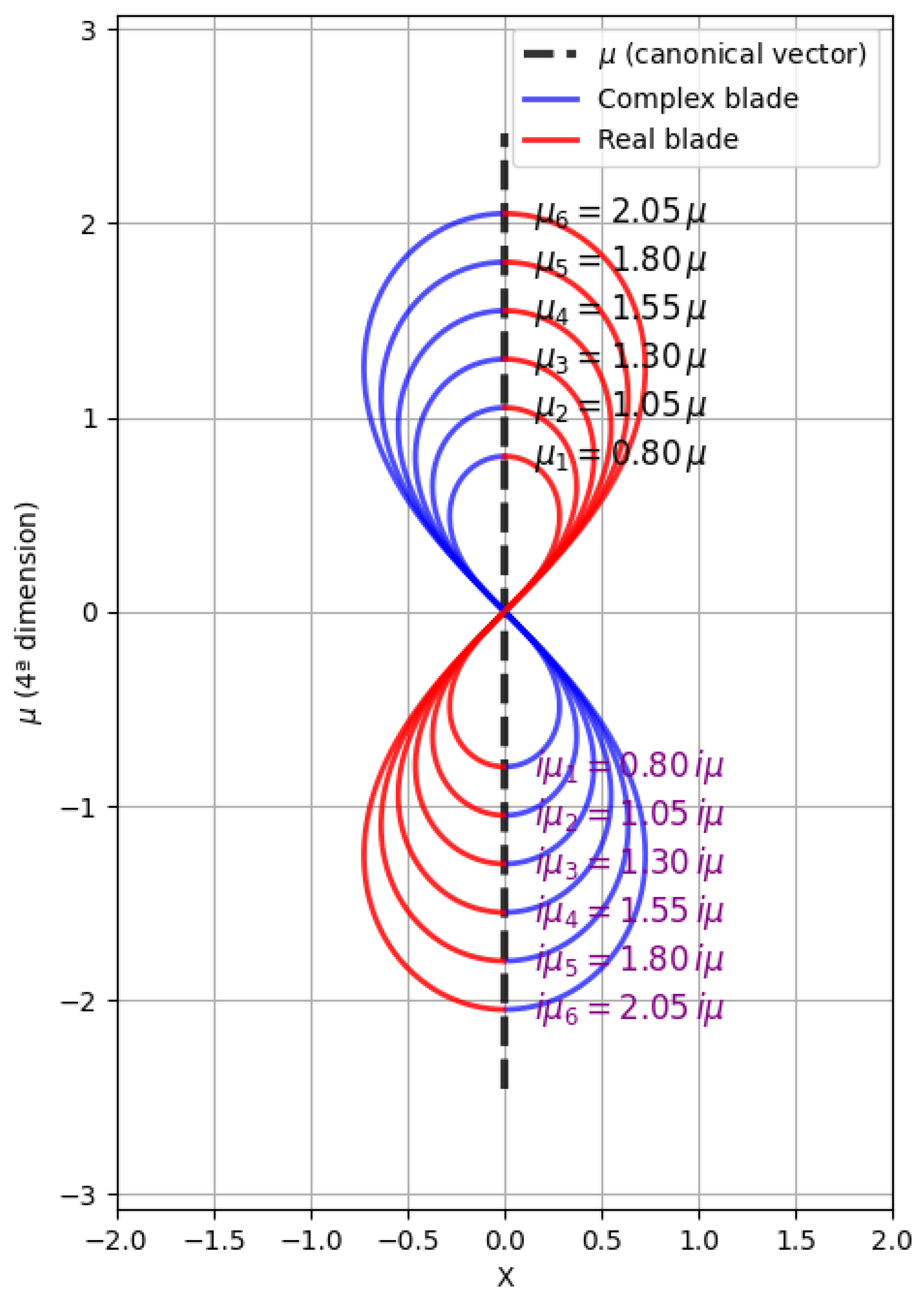
Figure 2.
– Euclidean-like behavior. Monte Carlo simulation of the Alpha Group dynamics. The trajectory is shown in 3D projection of the 4D state space. Color represents time evolution.
Figure 2.
– Euclidean-like behavior. Monte Carlo simulation of the Alpha Group dynamics. The trajectory is shown in 3D projection of the 4D state space. Color represents time evolution.
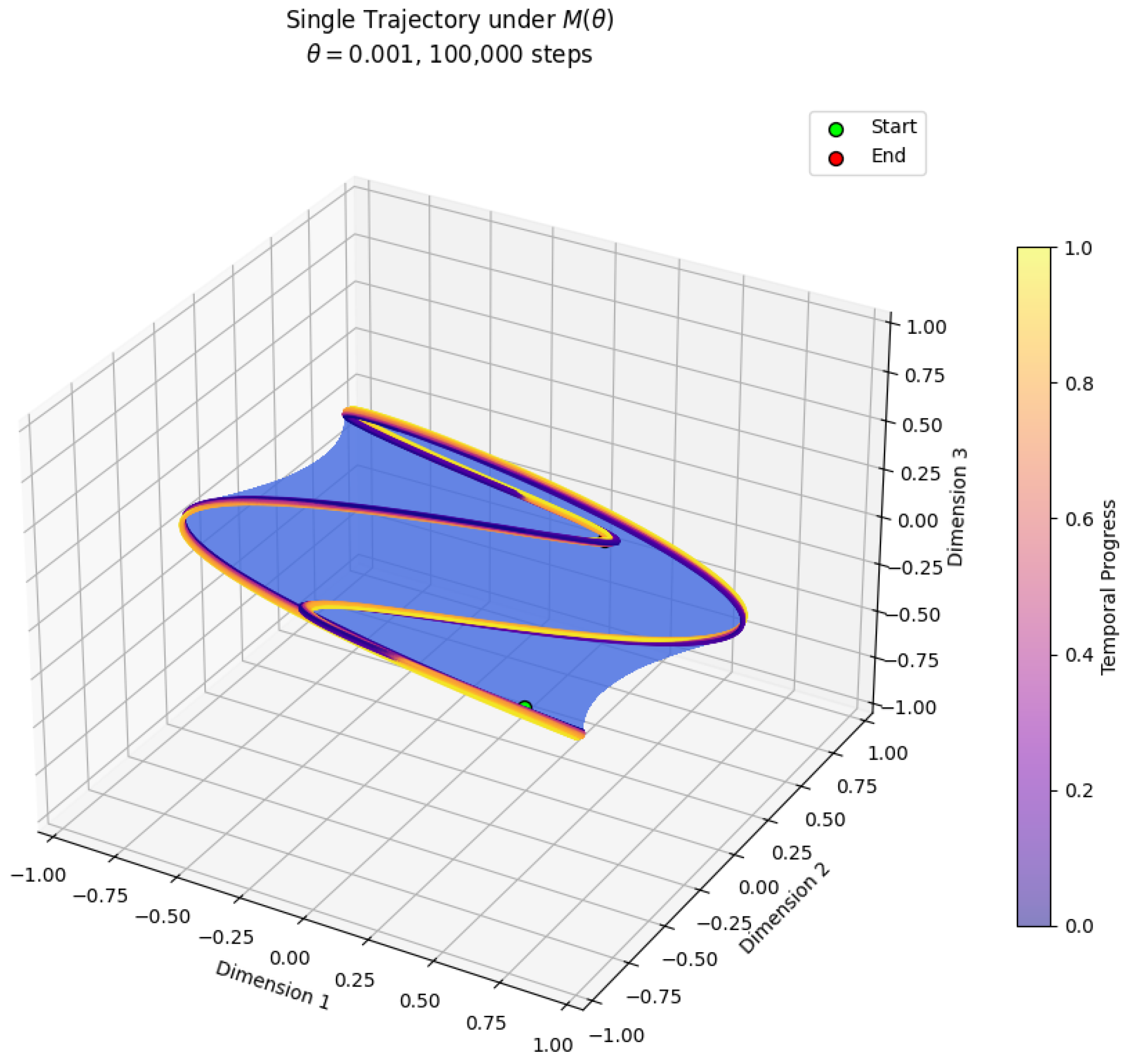
Figure 3.
– Intermediate rotation structure. Monte Carlo simulation of the Alpha Group dynamics. The trajectory is shown in 3D projection of the 4D state space. Color represents time evolution.
Figure 3.
– Intermediate rotation structure. Monte Carlo simulation of the Alpha Group dynamics. The trajectory is shown in 3D projection of the 4D state space. Color represents time evolution.
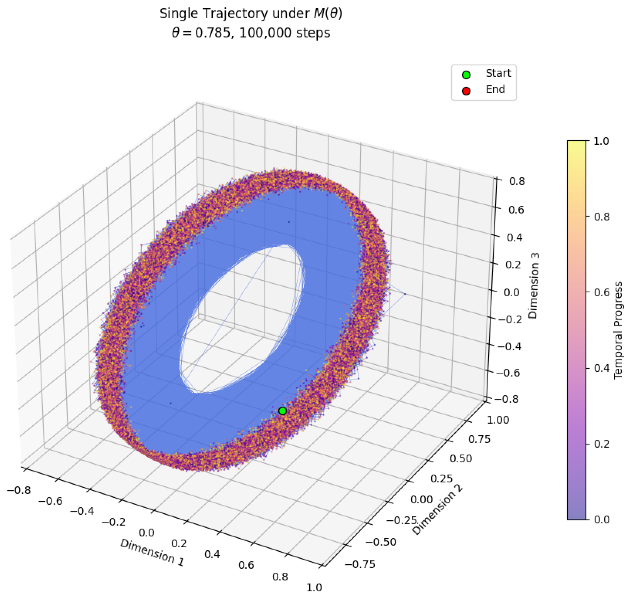
Figure 4.
– Boundary hyperbolic attractor. Monte Carlo simulation of the Alpha Group dynamics. The trajectory is shown in 3D projection of the 4D state space. Color represents time evolution.
Figure 4.
– Boundary hyperbolic attractor. Monte Carlo simulation of the Alpha Group dynamics. The trajectory is shown in 3D projection of the 4D state space. Color represents time evolution.
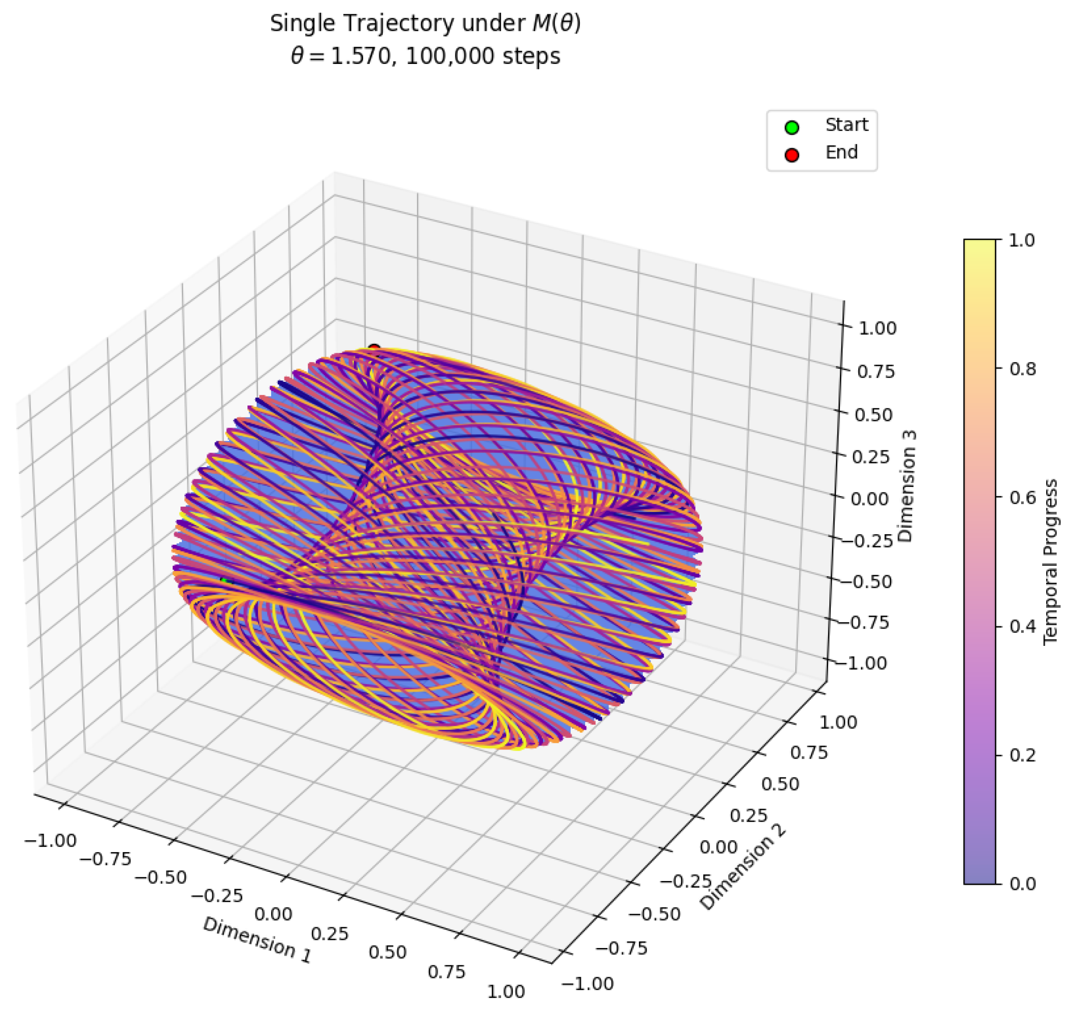

Table 1.
Comparison between the Alpha group and Classical Algebraic Groups/Quaternions.
| Group | Units | Key Relations | Topology/Geometry |
|---|---|---|---|
| Alpha group | Nontrivial projective structure, compactification to | ||
| Quaternion | topology, 4D algebra | ||
| Complex | i | topology, 2D field | |
| SU(2) | Double cover of SO(3) |
Disclaimer/Publisher’s Note: The statements, opinions and data contained in all publications are solely those of the individual author(s) and contributor(s) and not of MDPI and/or the editor(s). MDPI and/or the editor(s) disclaim responsibility for any injury to people or property resulting from any ideas, methods, instructions or products referred to in the content. |
© 2026 by the authors. Licensee MDPI, Basel, Switzerland. This article is an open access article distributed under the terms and conditions of the Creative Commons Attribution (CC BY) license (http://creativecommons.org/licenses/by/4.0/).
Copyright: This open access article is published under a Creative Commons CC BY 4.0 license, which permit the free download, distribution, and reuse, provided that the author and preprint are cited in any reuse.