
Submitted:
10 August 2025
Posted:
13 August 2025
You are already at the latest version
Abstract
Graph neural networks (GNNs) have shown prominent performance in predicting molecule properties. One aspect that is often overlooked in GNNs is the presence of patterns, such as functional groups, which are contained in substructures of molecules. There exist trivial patterns in molecules which can introduce an implicit bias, leading to false predictions. This can prevent models from properly learning the critical patterns that truly determine the properties of molecules. Therefore, we propose a hierarchical substructure-level method named Hypergraph-based Structure-aware Causal Graph Learning (HSCGL) to emphasize the causality between ground-truth labels and critical information including critical patterns and critical relationships from molecules, and to neglect trivial information including trivial patterns and trivial relationships from molecules by casual intervention strategy. In addition, to discover the cluster characteristics of patterns, we propose a structure-aware hypergraph learning to capture the structural information within each pattern. Extensive experiments and ablation study on real-world and synthetic datasets demonstrate the effectiveness of our HSCGL.
Keywords:
molecule property prediction
; hypergraph learning
; causal learning
1. Introduction
Predicting molecule properties is a prominent research area in drug discovery that has garnered significant attention in recent years [1,2]. The success of molecular graph representation learning with machine-learning based methods is evident in predicting molecule properties for graph classification tasks, including the evaluation of the therapeutic potential of drug candidates [3,4]. Molecular property prediction greatly benefits from nmigraph representation learning because molecular structures can be naturally modelled as graphs, where atoms are represented as nodes, and chemical bonds are represented as edges. Existing molecular graph representation learning methods, such as kernel-based methods [5,6] and pooling-based methods [7,8], are devoted to encoding graph information by conventional machine learning for graph representations. To alleviate the issue of lacking the ability to capture structural information in conventional methods, graph neural networks (GNNs) have been used in molecule property predictions. nmiHowever, existing GNN-based methods still suffer from the following limitations:
(1) Inadequate attention is given to patterns for cluster characteristics. GNNs take a node as an individual unit in their processing of graph data. Actually, nodes (i.e., atoms) can have explicit effects on molecular property prediction when they are jointly connected to a pattern as a cluster. Extensive research and empirical evidence have established that the properties of molecules are usually determined by patterns, which are contained in substructures of molecules, such as functional groups, retrosynthetically feasible chemical substructures, Bemis-Murcko scaffolds and valid connections [9,10]. Existing GNNs are unable to capture such a cluster characteristic from molecular graphs, where the patterns not only frequently exist but also tremendously affect the properties of molecules. Though recent research begins to exploit patterns, they still suffer from potential concerns of not considering the pattern as an entirety in modelling molecules [11].
(2) Lack of consideration of causality. Previous works [12,13] show that GNNs struggle to exploit the causality, which refers to causal information for capturing critical information from molecular graphs that truly determinates molecule property. Existing GNN-based methods usually capture trivial patterns (unhelpful for predictions) which frequently co-occur with critical patterns (helpful for predictions) in a graph, while neglecting to learn the critical patterns themselves. This phenomenon can be attributed to the implicit bias and noise by trivial patterns because of the frequent co-occurrence of trivial patterns alongside critical ones. Therefore, without causal intervention designs, GNNs are easily disturbed by spurious relations between input data and labels [14,15,16]. In other words, models mistakenly treat trivial patterns as the key to making predictions. For example, when classifying the mutagenic property, GNNs are expected to latch on critical patterns (e.g., nitrogen dioxides ()), rather than irrelevant trivial patterns (e.g., carbon rings) which frequently coexist with groups in real-world molecules. Existing models tend to perceive "carbon rings" as indicators of the "mutagenic" class simply because the majority of molecules with groups labelled as "mutagenic" are in the "carbon rings" context. Therefore, it is important to recognize the trivial patterns and take measures to ignore them to ensure more reliable predictions and improve model performance.
(3) Lack of consideration of 2-order relationships in molecules. Existing GNN-based methods [13,17,18] can not work well in real-world datasets because, in most cases, graphs own 1-order indiscernibility. This implies that the properties of graphs are strongly determined by patterns. Especially, molecules are governed by 2-order laws between patterns [19,20]. The 2-order relationship of a molecular graph refers to the relationships among the patterns, including critical relationships and trivial relationships. The frequent co-occurrence of critical and trivial relationships can also result in models mistakenly interpreting trivial relationships as critical ones. This misinterpretation can significantly impact model’s ability to generalize accurately. However, existing methods pay less attention to distinguishing critical relationships and trivial relationships, resulting in these methods being easily disturbed by a backdoor path between trivial relationships and ground-truth labels.
For example, the existence of group is a sufficient but non-necessary condition to judge whether a compound possesses mutagenicity because compounds with or group both arise the property of mutagenicity [21,22]. Moreover, it is also possible that the mutual sharpness/passivation between different functional groups may lead to advantageous/disadvantageous influences on the properties of molecular compounds. This type of data is ubiquitous in the real world. However, existing methods can not explicitly solve this problem well.
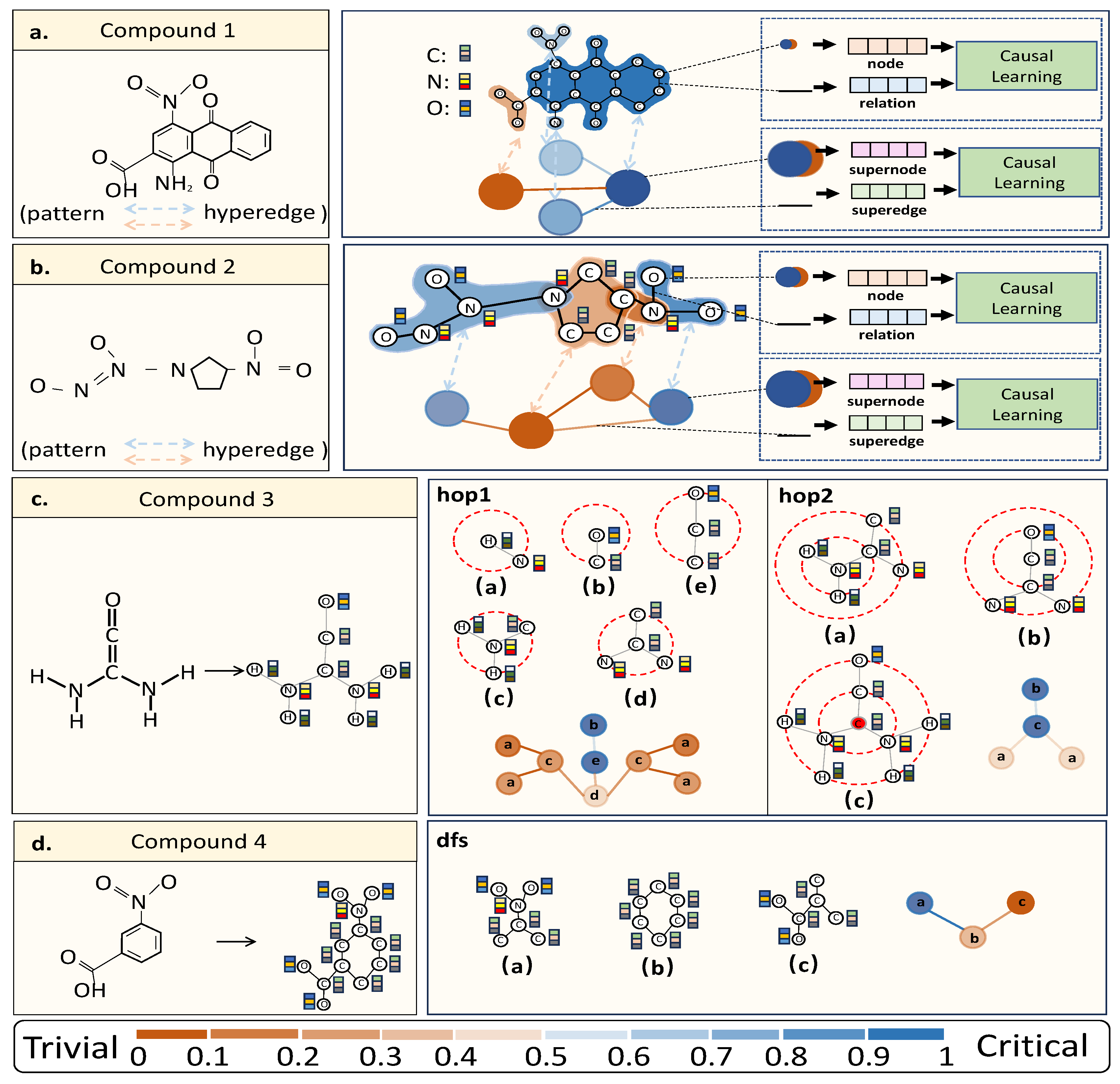
To further illustrate the 2-order relationship, we exemplify it with the compound 1 in Figure 3a. Both the presence of nitro, amino, and quinone functional groups significantly contribute to determining the toxicity of the molecule. For illustration purposes, we use a 2-dim one-hot vector to represent the molecular graph, e.g., the “nitro-only”, “quinone-only” and “nitro-quinone” represent , and , respectively. We need to learn an OR-gate-like classifier to classify , and into a class and classify into another one. And the connection between the nitro and quinone groups also has a positive impact on the overall toxicity of the molecule. In more complex cases, it is possible that the occurrence of two sub-critical patterns will lead to the property passivation. For example, the activity of conjugate unsaturated property will be decreased after double-bonded carbon groups () connect with Cl atoms, resulting in that we need to learn a XOR-gate-like classifier to classify and to a class and classify and to another one. Therefore, a high-order neural network is preferable to learn high-order structures among patterns from molecules.
To tackle these aforementioned limitations, we propose a novel hierarchical substructure-level method, which incorporates cluster characteristics, causal information and 2-order relationships. Our method, termed as Hypergraph-based Structure-aware Causal Graph Learning (HSCGL), aims to construct better graph embeddings for molecules by aggregating embeddings from critical information and eliminating the impact of embeddings from trivial information.
To solve the first limitation, our HSCGL leverages a hypergraph neural network (HNN) [11,21,22,23,24] to capture the cluster characteristics and pay more attention to explore the role of each pattern in the whole molecule. Our HSCGL clusters multiple nodes as a hyperedge which represents as a pattern to reconstruct a hypergraph. HNN is well-recognized as an ingenious tool in modelling a hypergraph for discovering the clustering characteristic among multiple connected nodes. However, it cannot exploit the structural information within each pattern. In molecules, different functional groups with exactly the same node set (also called functional group isomers, such as Monoolefins and cycloalkanes [25]) exhibit different molecular characteristics due to different structures. To solve this issue, our HSCGL proposes the structure-aware mechanism of hyperedges in molecular graphs to capture structural information within each pattern. In addition, the global-local mutual information mechanism is also considered to acquire discriminative embeddings by maximizing mutual information between the hyperedge embeddings and the whole-graph embeddings.
To solve the second limitation, HSCGL exploits the causal intervention strategy by causal learning to capture critical patterns while avoiding trivial patterns. Causal learning eliminates the model’s reliance on trivial patterns, thereby avoiding erroneous learning. This enhances the model’s robustness against distribution shifts of trivial patterns. We reveal that the trivial patterns open a backdoor path and serve as confounders in graph learning. We leverage the backdoor adjustments from causal theory to establish combinations between critical patterns and a range of trivial patterns from other molecules. By doing so, we promote stable predictions that are insensitive to variations in the distribution of trivial patterns. Our HSCGL emphasizes consistent relationships between critical patterns and ground-truth labels, regardless of changes in the distribution of trivial patterns. This allows us to mitigate the adverse effects of biased data and enhance the model’s ability to maintain reliable and robust predictions.
To solve the third limitation, our HSCGL captures 2-order critical relationships between patterns and eliminates 2-order trivial relationships by causal learning, where 2-order relationships refer to relationships between different patterns. We establish combinations between critical relationships and a series of trivial relationships from other molecules to support consistent predictions that remain robust to changes in the distribution of trivial relationships. Our approach emphasizes the enduring relationships between critical relationships and ground-truth labels, regardless of variations in the distribution of trivial relationships. Since HSCGL considers the patterns and 2-order relationships among these patterns, it is an extension of the 1-order method. It is noteworthy that our experiments have shown that 2-order relationships can effectively improve the expressive ability in our HSCGL.
Moreover, exploiting cluster characteristics for graph representations is a non-trivial solution to assist models in addressing the problem of the lack of interpretability of critical information. Our HSCGL distinguishes critical and trivial patterns of molecules and emerges respective attentions of different clusters or nodes by attention scores to show our interpretability and superiority over existing methods for molecule property prediction.
Our contributions are summarized as follows:
- We employ hypergraph neural networks to learn the molecular graph representations at the pattern level.
- We propose a structure-aware mechanism to capture the structural information within each pattern in hypergraph neural networks and introduce a self-supervised global-local mutual information mechanism by leveraging a well-designed discriminator to obtain more distinctive embeddings of graphs.
- We effectively capture critical patterns and critical relationships by utilizing the backdoor adjustment of causal learning, improving the generalization ability and performance of models.
- Our proposed HSCGL also facilitates the visualization of vital patterns for drug discovery, aiding researchers in identifying key components for effective drug design and development. Extensive experiments and ablation study on real-world and synthetic datasets demonstrate the effectiveness of our HSCGL.
2. Related Work
2.1. Causality in Graph Learning
Causal learning [26] is a widely recognized method for exploring the causal models from data. Causal learning encourages models to concentrate on critical features such as zebra colours and textures which are significant in zebra classification, while disregarding trivial ones like the image background which might be shortcut features in zebra prediction tasks, ultimately enhancing the model’s robustness against distribution shifts of trivial features. Unlike computer vision domains [27,28,29,30,31,32] and natural language domains [33,34,35,36,37,38], the applications of causal learning from causal theory in the graph representation learning community are still in their infancy. A few existing research studies have begun to emerge in graph learning by leveraging causal learning to balance the distribution shift and eliminate the adverse impacts of trivial features of graph data. For example, Zhao et al. [39] propose to generate approximate samples of different classes from a sample as counterfactual samples for graph learning to balance the distribution shift and improve the link prediction ability of graph-based models. Besides, Ma et al. [9] focus on estimating individual treatment effect (ITE) with consideration of group interaction on multiple nodes in a social group, and leverage causal intervention to construct counterfactual data for eliminating the adverse impacts of trivial features by causal learning in COVID-19 infection prediction. A causal attention method named CAL [40] considers splitting the whole graph into the causal and non-causal graphs at the node level, and can eliminate non-causal features as well as leverage causal features in the classification task by causal learning from causal theory in graph learning. Different from these existing models, our novel hierarchical substructure-level HSCGL first leverages causal learning in molecule graph learning, identifies cluster characteristics of patterns, and considers 2-order causal relationships between patterns.
2.2. Hypergraph in Improving Expressive Ability
While the conventional pairwise graph modelling in molecules effectively addresses a vast number of graph classification tasks, it falls short in capturing the comprehensive information of cluster interactions, which typically involve more than two nodes within each cluster. The hypergraph structure has been employed to model cluster characteristics among data. Hypergraph learning is first introduced by Zhou et al. [41] as a message propagation method on the hypergraph structure. In order to enhance the hypergraph learning performance, recent research has focused on incorporating a convolution operation and learning the weights of hyperedges. These approaches have possessed a significant impact on the modelling of data correlations. For example, Feng et al. [11] propose hypergraph neural networks (HNN, HNNP) to model beyond-pairwise complex correlations. They consider a convolution of hypergraph to capture the cluster characteristics for graph representation learning. In addition, Bai et al. [42] and Fan et al. [43] both introduce hypergraph attention neural network for homogeneous and heterogeneous hypergraph, respectively. However, the structural information within each hyperedge of the molecular graphs are hardly considered, and the aggregation of all the hyperedge embeddings for graph embeddings in existing works can potentially lead to over-smoothing issues. Therefore, we utilize hypergraph neural networks to learn cluster characteristics and structural information within each pattern, and introduce a self-supervised global-local mutual information mechanism by leveraging a well-designed discriminator to obtain more distinctive embeddings of molecular graphs.
3. Methods
To address the limitations of existing methods, we propose a hierarchical substructure-level method named Hypergraph-based Structure-aware Causal Graph Learning (HSCGL) for molecule property prediction. The overview of HSCGL is shown in Figure 1.
3.1. Notations
In this paper, scalars are denoted by normal alphabets, e.g., the total number of nodes, N; sets are denoted by calligraphy typeface alphabets, e.g., set of nodes, ; matrices are denoted by boldface uppercase alphabets, e.g., an adjacency matrix . We denote a graph by with the node set and edge set , where and . Let be the node embedding matrix of , where is the F-dimensional attribute vector of node . We use the adjacency matrix to denote the graph structure, where if edge , otherwise . Different from traditional graphs, a hypergraph consists of nodes and hyperedges, where each hyperedge could link multiple nodes. Given a hypergraph with and . Herein, each hyperedge e of the hyperedge set is formed by connecting multiple nodes. denotes an incidence matrix of the hypergraph , and its values are defined as . Each column of denotes a hyperedge, with a value of 1 indicating the presence of the respective node within that hyperedge.
3.2. Overview of HSCGL
Our proposed HSCGL consists of the following main steps: (1) Step I: Hypergraph Sketching. To represent patterns within molecules as well as capture cluster characteristics, our proposed HSCGL firstly performs hypergraph sketching, which includes three sub-steps: Step I-a: hyperedge construction for clustering multiple nodes as a hyperedge from the original input graph to reconstruct a newly hypergraph; Step I-b: hyperedge connection for building a newly sketched graph to acquire the association between hyperedges; Step I-c: embedding learning for effectively learning hyperedge embeddings by our structure-aware mechanism and global-local mutual information mechanism; (2) Step II: Causal Learning. To capture the critical patterns and critical relationships, our HSCGL splits all the statistical messages of the sketched graph, which is generated from the hypergraph sketching step, up into the critical and trivial message flows in both 1-order and 2-order paradigms. Our HSCGL proposes a causal intervention strategy that shields models from confounders of trivial information; (3) Step III: Predictions. Once the graph embeddings have been obtained, our HSCGL can predict the categories of molecules.
3.3. Step I: Hypergraph Sketching
In this subsection, we detail the three substeps of Step I: hyperedge construction, hyperedge connection and embedding learning, that aim at representing patterns by hyperedges as well as capturing the 2-order relationships between patterns.
3.3.1. Step I-a: Hyperedge Construction
Patterns are represented by hyperedges. Our HSCGL follows the well-known depth-first-search(dfs)-based and k-hop neighbourhood-based clustering methods [41] to construct hyperedges from an input molecular graph to form a hypergraph . These clustering methods generate a hyperedge to represent a pattern, e.g. valid connection or implicit functional group. Each hyperedge is built by linking every node itself and m nodes along the dfs-m path or their k-hop neighbours according to the adjacency matrix of the graph . After constructing the hyperedges, we can obtain hyperedges and the corresponding incidence matrix . Then, hypergraph neural networks (HNNs) are considered to capture the respective embeddings of patterns.
3.3.2. Step I-b: Hyperedge Connection
In order to reveal the relationships among patterns, our HSCGL constructs the connections of hyperedges and reconstructs a new sketched graph to view hyperedges and their connections as a new graph’s nodes and relations. We gather the hyperedges, which define distinct clusters, and use them to reconstruct this new sketched graph that captures the intrinsic relationships among patterns. Accordingly, we reconstruct the sketched graph as from the hypergraph by utilizing the hyperedges produced in step I-a, where and denote the supernode set and superedge set as the hyperedges and their relationships. The sketched graph forms superedges, i.e., the connectivity between supernodes, by taking into account the number of common nodes between two hyperedges and . The sketched graph contains a superedge when the number of intersection nodes in and meets or exceeds a predetermined threshold . Thus,
Alternatively, we can also define a weighted superedges by using the proportion of common nodes of and as weights to construct edge weights between supernodes. After constructing the sketched graph , we learn the hyperedge embedding from the relationships between patterns by graph neural networks, e.g., GCN and GAT.
3.3.3. Step I-c: Embedding Learning
In this subsection, our HSCGL applies the structure-aware mechanism within hyperedges and introduces the global-local mutual information mechanism between hyperedges and the whole graphs that is described in the following to learn refined node and pattern embeddings.
Structure-aware Mechanism. Despite HNNs being effective in capturing cluster characteristics, it is still ineffective in capturing the local geometric structures within hyperedges. To address this issue, we propose a structure-aware mechanism that is composed of a GNN method to better capture hyperedge structure.
In a hypergraph from , the original structure is observed and the definition of a hyperedge is:
where , represents a hyperedge, and denote the set of nodes and edges within the hyperedge, respectively.
Specifically, to capture the structural information from neighbourhoods in a hyperedge, our structure-aware mechanism follows an iterative aggregation (message passing) scheme to update node embeddings. For an L-layer GNN, the update function at the l-th layer is represented as:
where is the embedding of node at the l-th layer with , is a set of adjacent nodes to , and AGGREGATION and COMBINE are both basal component functions of GNN. Our HSCGL introduces the node updating function using an L-layer graph neural network (defined in Equation (3)). By doing so, we aim to capture the local geometric structural information within hyperedges, which could enhance the representational ability of HNN. In particular, given a node embedding vector , the node updating function can be expressed as
where denotes the normalized adjacency matrix, denotes the parameter of GNN, and denotes an activation function.
Considering the graph convolution operation, our mechanism can be written in followings:
where Equation (5) is the convolution version of Equation (4), and denote a degree matrix and a self-loop adjacency matrix in , respectively, and denote the inter-hyperedge convolution node embedding outputs and the parameter of convolution, respectively. denotes the local convolution for aggregating neighbour node embeddings. Referring to [11], our mechanism applied in HNNs can be written in the following form:
where denotes our newly structure-aware incidence matrix, ⊙ denotes Hadamard product, and CONCAT operation means to combine each incidence matrix of all hyperedges. The parameter combines the parameters of of HNNs and of convolution, where . denotes the diagonal matrix of node degrees, denotes the diagonal matrix of hyperedge degrees. Then, the node and hyperedge embeddings can directly learn from HNNs.
Global-local Mutual Information Mechanism. To obtain more distinctive embeddings of the hyperedges, we propose a global-local mutual information (MI) mechanism, a self-supervised method with positive/negative pairs in our HSCGL. The global-local MI mechanism aims to enhance the hyperedge embeddings. This mechanism maximizes the mutual information between local and global pairs, i.e., hyperedges embeddings and the whole-graph embeddings.
First, we follow [11] for the hyperedge embedding in HNNs:
Second, the whole-graph embeddings can be obtained by a READOUT function as follows:
After obtaining a hyperedge embedding and a whole-graph embedding R, we use the discriminator as shown below to determine whether and R are related.
where denotes an activation function, ⊕ represents the concat operation and denotes the learnable parameter. Finally, our global-local MI objective can be defined as a standard binary cross-entropy (BCE) loss:
where denotes the number of negative samples and is a molecular graph embedding of that does not belong to the class of whose graph embedding is . By maximizing the mutual information between and , the BCE loss measures the Jensen-Shannon divergence between the joint distribution (positive samples) and the product of marginals (negative samples) as to enhance hyperedge embeddings [44,45].
3.4. Step II: Causal Learning
After obtaining the hyperedge embeddings, which represent pattern embeddings, our HSCGL utilizes these embeddings to differentiate between critical and trivial patterns. In the following subsections, we provide a detailed explanation of how our HSCGL effectively minimizes the impact of irrelevant trivial patterns that could potentially mislead the final predictions.
3.4.1. Structural Causality in HNNs
To illustrate the causality in a molecule, we construct a Structural Causal Model (SCM) as shown in Figure 2. It presents the causalities among variables: graph data , overall critical information , overall trivial information , critical pattern , trivial pattern , critical relationships , trivial relationships , overall relationships , graph representation , and prediction , where the link between variables signifies a cause-effect relationship in which the cause influences the effect: cause → effect. We list the specific explanations of all relationships for SCM as follows:
- . A molecule graph possesses both and , which affect the prediction of differently. The variable denotes the overall critical information, including critical patterns and critical relationships, that truly reflect the intrinsic property of the graph data. While represents the overall trivial information that usually disturb to false predictions.
- , and . The overall critical information are composed of critical patterns , which are represented by hyperedges, and critical relationships . The same to the overall trivial information which are composed of trivial patterns , and trivial relationships .
- . This link indicates the 2-order relationship between critical patterns and between critical patterns and trivial patterns. So as .
- . The variable captures overall relationships, encompassing those between critical patterns, between trivial patterns, and between critical patterns and trivial patterns. Here, includes not only the 2-order trivial relationships , but the 2-order critical relationships , which guide predictions.
- . The variable is the embedding made of and in graph learning methods.
- . The classifier will make prediction based on the graph representation of the input graph .
3.4.2. Backdoor Adjustment
It is obvious that shielding HNNs from the confounder is the key to improve the expressive ability of graph learning in molecule graph classification. As the dotted lines shown in Figure 2, eliminating backdoor paths by causal intervention helps avoid disturbations from trivial information. Because the distribution is disturbed by trivial information, we instead model the target distribution , where e denotes a new embedding space. We need to achieve the graph embedding learning by eliminating the backdoor paths and . The backdoor path between critical information and prediction passes through trivial information and it leads to an incorrect causal effect in the model prediction from trivial information. In fact, we can exploit the do-calculus intervention from causal theory [46,47] on the variable to remove the backdoor paths by estimating . In order to calculate the distribution , we first make the following basical conclusions from the SCM:
- The marginal probability is not affected by the intervention. Thus, is equivalent to the vanilla probability . Similarly, the conditional probability is not affected by the intervention on so that is equivalent to the vanilla probability .
- Due to the intervention on , resulting in the independence of and , the conditional probability is equivalent to the probability .
- By refining and into the patterns and and the 2-order relationships and , we conclude that , and , , and .
Therefore, the backdoor adjustment can be described as:
where denotes the confounder set including trivial patterns and trivial relationships from other molecules. For the sake of discussion, we use and to represent and , respectively. Also, we use and to represent the critical set and the trivial set , respectively. Equation (11) is called backdoor adjustment [46], which truly eliminates the confounding effect on both trivial patterns and trivial relationships by generating counterfactual graphs to combine critical information in a molecule with different trivial information from other molecules. The process of causal intervention occurs in the same embedding space, and it ensures the invariance of other information when intervention, e.g. graph structure. In order to achieve interventions, we manipulate the graph data and consider an effective method to get rid of the restrictions when the confounder is commonly unobservable and hard to obtain. Therefore, we propose a 2-order causal intervention method in followings. Such a method can leverage not only 1-order but 2-order causal interventions of patterns and relationships.
3.4.3. Causal Intervention Strategy
Concretely, as the trivial information is not expected to affect our final predictions, we further add a constraint to better shield the prediction from the trivial information, and rewrite it as follows:
where is the dataset, t belongs to the confounder set including trivial patterns and trivial relationships from other molecules, and is the variance of a probability distribution, denotes the overall model parameters and is a small positive constant.
Hence, we define the critical loss and trivial loss to achieve prediction by critical information and neglect the trivial information of a molecule from Equation (12) as:
where and denote critical information embedding and trivial information embedding of , denotes the label of in dataset , and denotes the uniform distribution.
As shown in Equation (11), to alleviate the issue of the impossibility of intervening on the data level, e.g., changing a graph’s trivial part to generate counterfactual graphs, we follow [40] to make an implicit intervention on the embedding level in the 2-order paradigm. Inspired by their work, our newly backdoor adjustment is beneficial to alleviate the confounding effect. We not only consider the 1-order intervention but also consider the 2-order intervention to pair multiple critical information from a molecule with multiple trivial ones from other molecules to compose the "intervened graphs" with the implicit intervention method by the following loss:
where denotes a molecule and denotes another molecule from , is the predictive logits from an activation function on "implicit intervened graph" with 1-order () and 2-order information (); is the sum embedding c of all critical nodes embeddings from , but is the sum embedding of all trivial nodes from ; is the embedding of critical pattern from , but is the embedding of trivial pattern from ; and are critical and trivial relationships between patterns from and , respectively. is the estimated hierarchical set of the overall trivial information, which collects the appearing trivial patterns and relationships from training data. Likewise, is the estimated hierarchical set of the overall critical information from training data. Equation (14) is defined as the causal intervention loss, which ensures that the prediction of the intervention graph remains constant and stable across trivial information. This guarantees a steady prediction that remains unaffected by variations in the distribution of trivial patterns and trivial relationships.
3.5. Step III: Predictions
Finally, our HSCGL combines the critical and trivial loss and in Equation (13), the causal intervention loss in Equation (14), and the global-local MI loss in Equation (10) to form the final loss function for molecule property predictions. The final loss function of HSCGL is then defined as follows:
where , and control the contributions of the trivial graph information, the causal intervention and the global-local MI enhancement, respectively. Hence, HSCGL is trained to predict molecular graph properties while keeping discriminative pattern embeddings aware of 2-order structures.
4. Results
In this section, we aim to verify the performance of HSCGL in predicting molecule properties. We evaluate our proposed HSCGL for outperforming competitive molecular graph learning models by leveraging cluster characteristics, causal information, and 2-order relationships. Besides, our proposed HSCGL considers 2-order critical relationships and can achieve higher performance than those methods that only incorporate 1-order critical information. Specially, HSCGL can capture the critical patterns with significant information and insightful interpretations.
4.1. Datasets
We conduct extensive experiments on 7 real-world datasets, including MUTAG [48], NCI1 [49], PROTEINS [50], PTC (FR, FM, MM) [51], Mutagenicity [52] from TUDataset [53], and we also conduct experiments on 4 synthetic datasets, one publicly available original synthetic dataset and our three newly synthetic datasets designed from the original synthetic dataset, as in Figure (i, ii, iii, iv) to verify our generalization and expressive abilities in capturing critical patterns and critical relationships. These four synthetic datasets contain 2,000 samples per class with 4 classes, 6 classes, 2 classes and 2 classes, respectively. The publicly available original synthetic dataset as shown in Figure (i) is used for identifying four patterns (i.e., House, Cycle, Grid and Diamond) [54,55], and they are accompanied by different bias rates b or of trivial patterns, i.e., Tree or BA structure (as the same as the setting in [40]). The value b indicates the proportion of the trivial pattern (e.g. Tree structure) of the molecules of a class to all the molecules of that class, and indicates the proportion of the other trivial pattern (e.g. BA structure). This dataset is used to test that our HSCGL avoids performance perturbations caused by trivial patterns; The synthetic compounded dataset groups the molecules with every two of four critical patterns to a class, resulting in 6 different classes; The synthetic separated dataset differs significantly from the synthetic compounded dataset as it divides the four patterns into two distinct groups. Each group is assigned a specific class based on the presence of either one or both of the two patterns within it. The synthetic biased separated dataset unbalances two critical patterns by a bias rate based on the synthetic separated dataset, e.g., in Figure iv, where denotes the quantity proportion of different critical patterns with a same trivial pattern in a class. These three synthetic datasets collectively assess the model’s capability to mitigate diverse influences on trivial relationships. The task is to analyse different impacts of critical information and trivial information, and verify the ability to distinguish the trivial information.

Table 1.
Mean test accuracy (%) of graph classification methods. The best scores per dataset are marked in boldface and the second best scores are underlined. Statistically significant differences between HSCGL and DiffWire, between HSCGL and CAL, which are marked in the upper right-hand corner of HSCGL’s score and the lower right-hand corner of HSCGL’s score, respectively, are tested using a one-sided paired t-test and are denoted using • for = .01 and ∘ for = .05.
| Models | MUTAG | NCI1 | PROTEINS | PTC-FR | PTC-FM | PTC-MM | Mutagenicity |
|---|---|---|---|---|---|---|---|
| sGIN | 85.73 | 64.33 | 66.48 | 66.38 | 64.76 | 68.68 | 68.53 |
| MinCutNet | 88.83 | 72.31 | 76.73 | 67.51 | 65.44 | 67.56 | 78.33 |
| mewispool | 78.65 | 73.40 | 73.40 | 65.82 | 61.32 | 62.50 | 80.51 |
| dropGNN | 89.97 | 79.12 | 71.79 | 68.37 | 66.17 | 67.84 | 81.25 |
| 89.36 | 72.17 | 77.10 | 66.67 | 63.88 | 68.10 | 73.74 | |
| 88.86 | 70.19 | 76.83 | 67.11 | 63.31 | 67.20 | 73.30 | |
| 88.30 | 70.54 | 76.64 | 67.81 | 63.61 | 68.11 | 73.53 | |
| DiffWire | 88.27• | 71.36• | 76.64• | 67.46• | 63.33• | 68.42• | 73.55• |
| CAL | 89.83• | 81.90• | 68.39• | 66.45• | 67.65• | 83.05• | |
4.2. Experimental Settings
In our HSCGL, we perform 10-fold cross-validations with 10 random seeds on TUDatasets. Besides, we use GCN and GAT as GNN encoders with 128 hidden units on synthetic datasets. As for training parameters, we train the models for 100 epochs with a batch size of 128. For the proposed HSCGL, we search all the hyperparameters (, and as in Equation (15)) in [0.1, 1.0) with a step size of 0.1 and report the results with the best settings. We optimize all models with the Adam optimizer. All experiments are conducted on a server with NVIDIA 2080 Ti (11GB GPU).
4.3. Research Questions
The following research questions guide the remainder of the paper: (RQ1) Does our proposed HSCGL outperform competitive molecular graph learning baselines by leveraging causal information? (RQ2) Can the proposed HSCGL of 2-order form achieve enhanced performance than those methods that only incorporate 1-order information? (RQ3) How do those introduced components affect the performance of HSCGL? (RQ4) Does HSCGL capture the critical information with significant patterns and insightful interpretations?
4.4. RQ1: Evaluation for Causality
We conduct experiments to evaluate our proposed HSCGL for outperforming competitive molecular graph learning models by leveraging causal information.
Figure 3.
Examples to showcase the importance of different patterns in four compounds. Our HSCGL can effectively distinguish between critical and trivial information at the 2-order level, enabling a more comprehensive understanding of the molecular structure and its properties.
Figure 3.
Examples to showcase the importance of different patterns in four compounds. Our HSCGL can effectively distinguish between critical and trivial information at the 2-order level, enabling a more comprehensive understanding of the molecular structure and its properties.
In Table 1, we report the results of existing models and our HSCGL to show that our HSCGL help achieve superior performance on real-world datasets. Since these datasets involve implicit or unobserved irregular critical patterns, we can conclude that HSCGL can leverage the critical information and eliminate backdoor paths between ground-truth labels and trivial information. In Table 2i, we present the results of GCN, GAT, the variant enhanced by a causal method, i.e., CAL, and the variant enhanced by considering cluster characteristics and 2-order critical relationships, i.e., our HSCGL, on the original synthetic datasets with a different bias rate b. We aim to examine the model’s ability to mine critical patterns and avoid trivial patterns. As shown in Table 2i, our proposed HSCGL can achieve enhanced effectiveness in modelling biased dataset by leveraging the “Tree”/“BA” trivial patterns [54,55] of different rates in a class as the confounder compared with all other baselines. Specifically, our HSCGL is designed to pay more attention to critical patterns, which can model the dataset distribution well regardless of the distribution of trivial patterns, especially in the extreme bias conditions, i.e., the bias rate b = 0.1 or 0.9. Therefore, our HSCGL can achieve better generalization.
We visualize the attention weights of patterns in the molecular graphs from the four compounds in Figure 3. An attribution value close to 1 indicates that the corresponding pattern plays a critical role in the prediction, while an attribution value close to 0 suggests that the pattern has minimal influence on the prediction. As shown in Figure 3a, we investigate the causal relationship of HSCGL in the toxicity analysis, which is of significant concern in drug development due to its potential harm to human health. A molecule may contain multiple toxic groups, such as compound 1 with three toxic groups: aromatic nitro group, aromatic amino group, and quinone group. However, current methods often attribute the phenyl ring as the primary toxic group due to its frequent co-occurrence with the nitro group. Conversely, these models consider the amino group to be less significant in terms of toxicity, as they finish the prediction through other signature toxic groups for simplicity. This phenomenon leads models to overlook the presence of amino groups in the prediction process. These lead to the misconception that the phenyl ring is predominantly toxic, while the amino groups are not. Based on our results, as illustrated in Figure 3a, the nitro, amino, and quinone groups positively contribute to enhancing toxicity prediction. Similarly, the carboxyl groups also aid in enhancing detoxification prediction. This aligns with existing research indicating that aromatic nitro, aromatic amino, and quinone groups are identified as toxic, while the carboxyl group is associated with detoxification. The underlying issue lies in the fact that not only do these individual toxic groups impact the toxicity prediction of the entire molecule, but the 2-order relationships in molecules play a crucial role. Additionally, the attention scores for the relationships between these groups indicate that the relationship between quinone and amino groups is particularly instrumental in molecule property prediction.
Similarly, in the three remaining compounds 2, 3 and 4 depicted in Figure 3, our proposed HSCGL effectively captures critical information that greatly enhances the model’s performance. (b) The compound 2 is composed of nitro, carbon-nitrogen, piperidine-like and azooxy patterns. Our proposed HSCGL learns to make a causal view of 2-order relationships, including the relationships between azooxy and piperidine-like groups that confounds the predictions of the mutagenic property. (c) During the Hyperedge Construction phase, the compound 3 utilizes both 1-hop and 2-hop neighbourhood-based clustering methods to construct hyperedges from an input molecular graph. (d) The compound 4 employs a depth-first-search(dfs)-based clustering method to construct hyperedges from an input molecular graph. As a result, HSCGL can effectively discern between critical and trivial information, leading to improved performance in molecule prediction.
It needs to be explained that, when comparing the artificial construction of supernodes in Figure 3a-b, where each supernode is expertly designed, it becomes clear that this method incurs significant labour costs and is not cost-effective, particularly in large-scale datasets. To address this limitation, we proposed HSCGL can automate the construction of supernodes. Our approach has the potential to reveal implicit patterns, including those that may currently remain undiscovered but play a crucial role in predicting molecular properties. As illustrated in Figure 3c-d, during the Hyperedge Construction phase, our HSCGL is capable of learning these underlying patterns without the need for manual labelling. Additionally, HSCGL excels at distinguishing between critical and trivial patterns, offering a more efficient and effective solution while reducing the need for human labour.
4.5. RQ2: Evaluation on 2-order Form
To explain that our proposed HSCGL of 2-order form can identify critical relationships among patterns and achieve enhanced performance than those methods that only incorporate 1-order information, we create three new synthetic datasets: synthetic compounded dataset, synthetic separated dataset and synthetic biased separated dataset. By conducting experiments on these synthetic datasets, we aim to evaluate how our HSCGL obtains 2-order critical relationships among patterns to achieve better performance than other methods. (1) In Table 2ii, models need to perform as an AND-gate-like function to classify a molecule to a class when the molecule includes every two of four critical patterns, e.g., "House" and "Grid" both connect with "Tree" in this molecule, otherwise to classify to another class. However, CAL [40] does not perform well because it only captures the 1-order information. Instead, our proposed HSCGL is well qualified for this situation. (2) In Table 2iii, we conduct experiments on the synthetic separated dataset. Models need to perform as an OR-gate-like function to classify a molecule to a class when the presence of either one or both of the two patterns within the molecule, otherwise to classify to another class. As a result, our HSCGL also shows better performance. (3) In Table 2iv, we conduct experiments on the synthetic biased separated dataset with to prove the performance of our HSCGL. Our HSCGL consistently produces enhanced performances, ensures the generalization under a 2-order paradigm, and effectively eliminates the backdoor paths between ground-truth labels and trivial patterns. Therefore, experiments on the three synthetic datasets demonstrate that our HSCGL can capture the 2-order critical information of data and obtain superior improvement of performance.
It is worth noting that the performance of a biased dataset (e.g., b = 0.3) may seldom be better than that of the unbiased dataset (b = 0.5) in Table 2 due to the strong similarity between two critical patterns, i.e., the "House" pattern is actually a substructure of the "Diamond" one.
4.6. RQ3: Ablation Study
We conduct the following experiments in this subsection to explore the impacts of causality, HNN, different construction methods and different components of our HSCGL.
Effectiveness of causality and HNN. The experiments of both hypergraph learning which is in the absence of causal steps and causality which is in the absence of HNN but preserving supernode construction in our HSCGL are shown in Table 3. (1) Our experiments clearly indicate a significant decline in performance when the causal step is removed. We conclude that causality truly improves performance in real datasets (e.g. +1.78% on PTC-FR) and synthetic datasets (e.g. +1.98% on synthetic separated datasets). (2) In the absence of HNN, we still conduct supernodes using existing construction methods (hop1 or hop2) and we approximate each supernode embedding as the mean of the embeddings of nodes. Without HNN, this is a rough estimation method with a loss in accuracy. The experimental results demonstrate that 2-order group characteristics by HNN indeed work.
Different construction methods of superedges. Different construction methods of superedge determine the connection relationships between supernodes. We test our HSCGL with different thresholds of 1, 3, 5 as well as weighted superedges. denotes the minimal number of common nodes when existing a link between two hyperedges. From Figure 4a, we observe that the threshold value itself has a marginal effect on the final performance. Noticeably, on both datasets, our HSCGL benefits from a lower threshold value, i.e., =1 or 3. This is because both MUTAG and PROTEINS are relatively small datasets, which means a higher threshold might lead to too sparse superedge connections. Such a sparsely connected hypergraph may suffer from the undertraining issue. Additionally, when =1, it results in excessively dense superedge connections and may occur over-smoothing issue. Therefore, we can conclude that a lower threshold is more favourable on small datasets and when =3, our HSCGL reach better results.
Different components. We explore the effectiveness of each component as shown in Figure 4b, including the structure-aware and global-local MI mechanisms, 1-order and 2-order causal information. We have verified several different hyperedge construction methods (dfs5, dfs10, hop1 and hop2) for evaluating performance of different components. Among them, we find that 1-order and 2-order causal information provide relatively more important support for the improvement of performance on molecular graph classification.
Figure 5.
The visualizations of HSCGL on synthetic separated dataset.
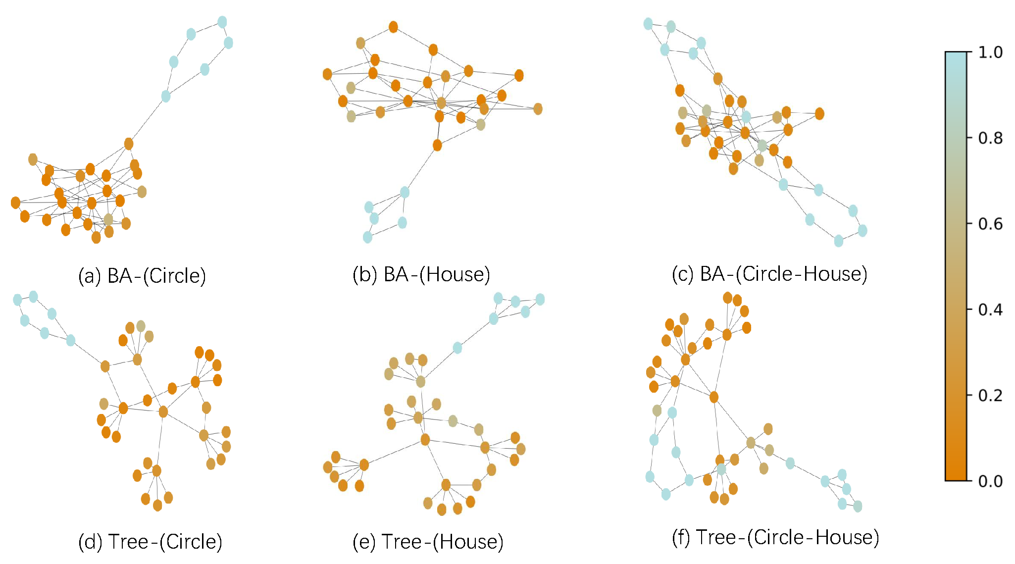
4.7. RQ4: Visual Interpretations
To additionally explain that HSCGL can capture critical patterns for insightful interpretations, we also visualize critical and trivial patterns in synthetic separated datasets to show the effectiveness of our HSCGL. We plot hyperedge attention areas by attention scores of HSCGL in Figure 5. In synthetic separated datasets, our HSCGL can well distinguish the critical patterns (i.e., Circle and House) with an attention score close to 1, while discarding the unimportant trivial patterns (i.e., Tree and BA) with an attention score close to 0.
5. Discussions
We propose Hypergraph-based Structure-aware Causal Graph Learning to distinguish between critical and trivial patterns and learn to accurately predict molecule properties. Our HSCGL offers explanations that align with the understanding of chemists, thereby avoiding misleading inferences arising from trivial patterns in the prediction of molecule properties. Consequently, we are confident that HSCGL empowers chemists to impartially identify critical patterns and extract vital information from molecules.
Our HSCGL leverages cluster characteristics, causal information, and 2-order relationships to enhance graph embeddings for molecules. By integrating embeddings from critical patterns, our method implicitly learns critical information including critical patterns and critical relationships. While HSCGL has shown promising performance, it may still have some limitations. Firstly, capturing 2-order critical relationships between patterns which are remotely linked in a molecule poses challenges. While our HSCGL excels in distinguishing critical information at both the 1-order and 2-order levels, it may not work well when dealing with complex molecules. Our HSCGL can indeed capture long-distance dependencies between patterns, but it is not yet optimal for capturing relationships between distant patterns. Efforts can be considered in the future to improve the model’s ability to capture long-distance patterns and enhance its overall performance in these scenarios. Secondly, we acknowledge that there exist unsupervised estimations in constructing hyperedges as patterns. Adjusting these patterns in combination with existing knowledge has the potential to further improve the model’s performance. Nevertheless, it is important to note that incorporating existing knowledge can be a complex and costly endeavour. This aspect also opens up avenues for future research, such as incorporating expert knowledge or exploring the use of pre-training methods to introduce additional domain-specific information. These approaches can be beneficial for drug discovery and they have the potential to further enhance the model’s performance by leveraging external knowledge sources.
6. Conclusions
In the field of molecule property prediction, patterns such as Bemis-Murcko scaffolds and functional groups play a crucial role in determining molecular properties. Additionally, there exist critical patterns and critical relationships between patterns which truly determine molecule property. Conversely, the presence of trivial patterns and trivial relationships between patterns which lead to an implicit bias, ultimately having a detrimental impact on molecule property prediction. In our research, we address the aforementioned challenges by leveraging cluster characteristics, causal information, and 2-order relationships in molecule property prediction. We propose Hypergraph-based Structure-aware Causal Graph Learning (HSCGL) for molecular graph representation learning. We first employ a hypergraph neural network to learn the molecular graph representation at the pattern level. Additionally, we propose a structure-aware mechanism to capture the structural information within each pattern. We effectively capture critical patterns and critical relationships by utilizing the backdoor adjustment of causal learning, improving the generalization ability and performance of models. Furthermore, our proposed HSCGL also facilitates the visualization of vital patterns for drug discovery, aiding researchers in identifying key components for effective drug design and development. Extensive experiments and ablation study on real-world and synthetic datasets demonstrate the effectiveness of our HSCGL.
References
- Fang, Y.; Zhang, Q.; Zhang, N.; Chen, Z.; Zhuang, X.; Shao, X.; Fan, X.; Chen, H. Knowledge graph-enhanced molecular contrastive learning with functional prompt. Nature Machine Intelligence, 2023, pp. 1–12.
- Wu, Z.; Wang, J.; Du, H.; Jiang, D.; Kang, Y.; Li, D.; Pan, P.; Deng, Y.; Cao, D.; Hsieh, C.Y.; et al. Chemistry-intuitive explanation of graph neural networks for molecular property prediction with substructure masking. Nature Communications 2023, 14, 2585. [Google Scholar] [CrossRef] [PubMed]
- Zhang, Z.; Liu, Q.; Wang, H.; Lu, C.; Lee, C.K. Motif-based graph self-supervised learning for molecular property prediction. Advances in Neural Information Processing Systems 2021, 34, 15870–15882. [Google Scholar]
- Wang, Z.; Liu, M.; Luo, Y.; Xu, Z.; Xie, Y.; Wang, L.; Cai, L.; Qi, Q.; Yuan, Z.; Yang, T.; et al. Advanced graph and sequence neural networks for molecular property prediction and drug discovery. Bioinformatics 2022, 38, 2579–2586. [Google Scholar] [CrossRef]
- Shervashidze, N.; Schweitzer, P.; Van Leeuwen, E.J.; Mehlhorn, K.; Borgwardt, K.M. Weisfeiler-lehman graph kernels. Journal of Machine Learning Research 2011, 12. [Google Scholar]
- Yanardag, P.; Vishwanathan, S. Deep graph kernels. In Proceedings of the Proceedings of the 21th ACM SIGKDD international conference on knowledge discovery and data mining, 2015, pp. 1365–1374.
- Ying, Z.; You, J.; Morris, C.; Ren, X.; Hamilton, W.; Leskovec, J. Hierarchical graph representation learning with differentiable pooling. Advances in neural information processing systems 2018, 31. [Google Scholar]
- Zhang, M.; Cui, Z.; Neumann, M.; Chen, Y. An end-to-end deep learning architecture for graph classification. In Proceedings of the Proceedings of the AAAI conference on artificial intelligence, 2018, Vol. 32.
- Ma, J.; Wan, M.; Yang, L.; Li, J.; Hecht, B.; Teevan, J. Learning Causal Effects on Hypergraphs. In Proceedings of the Proceedings of the 28th ACM SIGKDD Conference on Knowledge Discovery and Data Mining, 2022, pp. 1202–1212.
- Knyazev, B.; Taylor, G.W.; Amer, M. Understanding attention and generalization in graph neural networks. Advances in neural information processing systems 2019, 32. [Google Scholar]
- Feng, Y.; You, H.; Zhang, Z.; Ji, R.; Gao, Y. Hypergraph neural networks. In Proceedings of the Proceedings of the AAAI conference on artificial intelligence, 2019, Vol. 33, pp. 3558–3565.
- Dwivedi, V.P.; Joshi, C.K.; Laurent, T.; Bengio, Y.; Bresson, X. Benchmarking graph neural networks. arXiv preprint, arXiv:2003.00982 2020.
- Kipf, T.N.; Welling, M. Semi-supervised classification with graph convolutional networks. arXiv preprint, arXiv:1609.02907 2016.
- Wang, X.; Wu, Y.; Zhang, A.; Feng, F.; He, X.; Chua, T.S. Reinforced Causal Explainer for Graph Neural Networks. IEEE Transactions on Pattern Analysis and Machine Intelligence 2022. [Google Scholar] [CrossRef] [PubMed]
- Wang, X.; Wu, Y.; Zhang, A.; He, X.; Chua, T.S. Towards multi-grained explainability for graph neural networks. Advances in Neural Information Processing Systems 2021, 34, 18446–18458. [Google Scholar]
- Wu, Y.X.; Wang, X.; Zhang, A.; He, X.; Chua, T.S. Discovering invariant rationales for graph neural networks. arXiv preprint, arXiv:2201.12872 2022.
- Veličković, P.; Cucurull, G.; Casanova, A.; Romero, A.; Lio, P.; Bengio, Y. Graph attention networks. arXiv preprint, arXiv:1710.10903 2017.
- Hamilton, W.; Ying, Z.; Leskovec, J. Inductive representation learning on large graphs. Advances in neural information processing systems 2017, 30. [Google Scholar]
- Courcelle, B. On the Expression of Graph Properties in some Fragments of Monadic Second-Order Logic. Descriptive complexity and finite models 1996, 31, 33–62. [Google Scholar]
- Wang, Z.; Ji, S. Second-order pooling for graph neural networks. IEEE Transactions on Pattern Analysis and Machine Intelligence 2020. [Google Scholar] [CrossRef]
- Gao, Y.; Feng, Y.; Ji, S.; Ji, R. HGNN +: General Hypergraph Neural Networks. IEEE Transactions on Pattern Analysis and Machine Intelligence 2022. [Google Scholar] [CrossRef]
- Alam, M.T.; Ahmed, C.F.; Samiullah, M.; Leung, C.K.S. Discovering Interesting Patterns from Hypergraphs. ACM Transactions on Knowledge Discovery from Data 2023, 18, 1–34. [Google Scholar] [CrossRef]
- Balalau, O.; Bonchi, F.; Chan, T.H.; Gullo, F.; Sozio, M.; Xie, H. Finding Subgraphs with Maximum Total Density and Limited Overlap in Weighted Hypergraphs. ACM Transactions on Knowledge Discovery from Data 2024. [Google Scholar] [CrossRef]
- Li, M.; Zhang, Y.; Li, X.; Zhang, Y.; Yin, B. Hypergraph transformer neural networks. ACM Transactions on Knowledge Discovery from Data 2023, 17, 1–22. [Google Scholar] [CrossRef]
- Hsu, C.S. Definition of hydrogen deficiency for hydrocarbons with functional groups. Energy & fuels 2010, 24, 4097–4098. [Google Scholar]
- Yao, L.; Chu, Z.; Li, S.; Li, Y.; Gao, J.; Zhang, A. A survey on causal inference. ACM Transactions on Knowledge Discovery from Data (TKDD) 2021, 15, 1–46. [Google Scholar] [CrossRef]
- Tang, K.; Huang, J.; Zhang, H. Long-tailed classification by keeping the good and removing the bad momentum causal effect. Advances in Neural Information Processing Systems 2020, 33, 1513–1524. [Google Scholar]
- Huang, J.; Qin, Y.; Qi, J.; Sun, Q.; Zhang, H. Deconfounded visual grounding. In Proceedings of the Proceedings of the AAAI Conference on Artificial Intelligence, 2022, Vol. 36, pp. 998–1006.
- Qi, J.; Niu, Y.; Huang, J.; Zhang, H. Two causal principles for improving visual dialog. In Proceedings of the Proceedings of the IEEE/CVF conference on computer vision and pattern recognition, 2020, pp. 10860–10869.
- Niu, Y.; Tang, K.; Zhang, H.; Lu, Z.; Hua, X.S.; Wen, J.R. Counterfactual vqa: A cause-effect look at language bias. In Proceedings of the Proceedings of the IEEE/CVF Conference on Computer Vision and Pattern Recognition, 2021, pp. 12700–12710.
- Yang, X.; Zhang, H.; Cai, J. Deconfounded image captioning: A causal retrospect. IEEE Transactions on Pattern Analysis and Machine Intelligence 2021. [Google Scholar] [CrossRef]
- Zhang, D.; Zhang, H.; Tang, J.; Hua, X.S.; Sun, Q. Causal intervention for weakly-supervised semantic segmentation. Advances in Neural Information Processing Systems 2020, 33, 655–666. [Google Scholar]
- Li, M.; Feng, F.; Zhang, H.; He, X.; Zhu, F.; Chua, T.S. Learning to Imagine: Integrating Counterfactual Thinking in Neural Discrete Reasoning. In Proceedings of the Proceedings of the 60th Annual Meeting of the Association for Computational Linguistics (Volume 1: Long Papers), 2022, pp. 57–69.
- Cao, B.; Lin, H.; Han, X.; Liu, F.; Sun, L. Can Prompt Probe Pretrained Language Models? Understanding the Invisible Risks from a Causal View. arXiv preprint, arXiv:2203.12258 2022.
- Qian, C.; Feng, F.; Wen, L.; Ma, C.; Xie, P. Counterfactual inference for text classification debiasing. In Proceedings of the Proceedings of the 59th Annual Meeting of the Association for Computational Linguistics and the 11th International Joint Conference on Natural Language Processing (Volume 1: Long Papers), 2021, pp. 5434–5445.
- Feder, A.; Keith, K.A.; Manzoor, E.; Pryzant, R.; Sridhar, D.; Wood-Doughty, Z.; Eisenstein, J.; Grimmer, J.; Reichart, R.; Roberts, M.E.; et al. Causal inference in natural language processing: Estimation, prediction, interpretation and beyond. Transactions of the Association for Computational Linguistics 2022, 10, 1138–1158. [Google Scholar] [CrossRef]
- Keith, K.A.; Jensen, D.; O’Connor, B. Text and causal inference: A review of using text to remove confounding from causal estimates. arXiv preprint, arXiv:2005.00649 2020.
- Abraham, E.D.; D’Oosterlinck, K.; Feder, A.; Gat, Y.; Geiger, A.; Potts, C.; Reichart, R.; Wu, Z. CEBaB: Estimating the causal effects of real-world concepts on NLP model behavior. Advances in Neural Information Processing Systems 2022, 35, 17582–17596. [Google Scholar]
- Zhao, T.; Liu, G.; Wang, D.; Yu, W.; Jiang, M. Learning from counterfactual links for link prediction. In Proceedings of the International Conference on Machine Learning. PMLR; 2022; pp. 26911–26926. [Google Scholar]
- Sui, Y.; Wang, X.; Wu, J.; Lin, M.; He, X.; Chua, T.S. Causal attention for interpretable and generalizable graph classification. In Proceedings of the Proceedings of the 28th ACM SIGKDD Conference on Knowledge Discovery and Data Mining, 2022, pp. 1696–1705.
- Zhou, D.; Huang, J.; Schölkopf, B. Learning with hypergraphs: Clustering, classification, and embedding. Advances in neural information processing systems 2006, 19. [Google Scholar]
- Bai, S.; Zhang, F.; Torr, P.H. Hypergraph convolution and hypergraph attention. Pattern Recognition 2021, 110, 107637. [Google Scholar] [CrossRef]
- Fan, H.; Zhang, F.; Wei, Y.; Li, Z.; Zou, C.; Gao, Y.; Dai, Q. Heterogeneous hypergraph variational autoencoder for link prediction. IEEE Transactions on Pattern Analysis and Machine Intelligence 2021, 44, 4125–4138. [Google Scholar] [CrossRef]
- Nowozin, S.; Cseke, B.; Tomioka, R. f-gan: Training generative neural samplers using variational divergence minimization. Advances in neural information processing systems 2016, 29. [Google Scholar]
- Velickovic, P.; Fedus, W.; Hamilton, W.L.; Liò, P.; Bengio, Y.; Hjelm, R.D. Deep graph infomax. ICLR (Poster) 2019, 2, 4. [Google Scholar]
- Pearl, J. Interpretation and identification of causal mediation. Psychological methods 2014, 19, 459. [Google Scholar] [CrossRef] [PubMed]
- Pearl, J.; et al. Models, reasoning and inference. Cambridge, UK: CambridgeUniversityPress 2000, 19. [Google Scholar]
- Debnath, A.K.; Lopez de Compadre, R.L.; Debnath, G.; Shusterman, A.J.; Hansch, C. Structure-activity relationship of mutagenic aromatic and heteroaromatic nitro compounds. correlation with molecular orbital energies and hydrophobicity. Journal of medicinal chemistry 1991, 34, 786–797. [Google Scholar] [CrossRef]
- Wale, N.; Watson, I.A.; Karypis, G. Comparison of descriptor spaces for chemical compound retrieval and classification. Knowledge and Information Systems 2008, 14, 347–375. [Google Scholar] [CrossRef]
- Dobson, P.D.; Doig, A.J. Distinguishing enzyme structures from non-enzymes without alignments. Journal of molecular biology 2003, 330, 771–783. [Google Scholar] [CrossRef] [PubMed]
- Bai, Y.; Ding, H.; Qiao, Y.; Marinovic, A.; Gu, K.; Chen, T.; Sun, Y.; Wang, W. Unsupervised inductive graph-level representation learning via graph-graph proximity. arXiv preprint, arXiv:1904.01098 2019.
- Zhang, Z.; Bu, J.; Ester, M.; Zhang, J.; Yao, C.; Yu, Z.; Wang, C. Hierarchical graph pooling with structure learning. arXiv preprint, arXiv:1911.05954 2019.
- Morris, C.; Kriege, N.M.; Bause, F.; Kersting, K.; Mutzel, P.; Neumann, M. Tudataset: A collection of benchmark datasets for learning with graphs. arXiv preprint, arXiv:2007.08663 2020.
- Ying, Z.; Bourgeois, D.; You, J.; Zitnik, M.; Leskovec, J. Gnnexplainer: Generating explanations for graph neural networks. Advances in neural information processing systems 2019, 32. [Google Scholar]
- Barabási, A.L.; Albert, R. Emergence of scaling in random networks. science 1999, 286, 509–512. [Google Scholar] [CrossRef] [PubMed]
Figure 1.
The overview of our proposed Hypergraph-based Structure-aware Causal Graph Learning (HSCGL) model.
Figure 1.
The overview of our proposed Hypergraph-based Structure-aware Causal Graph Learning (HSCGL) model.
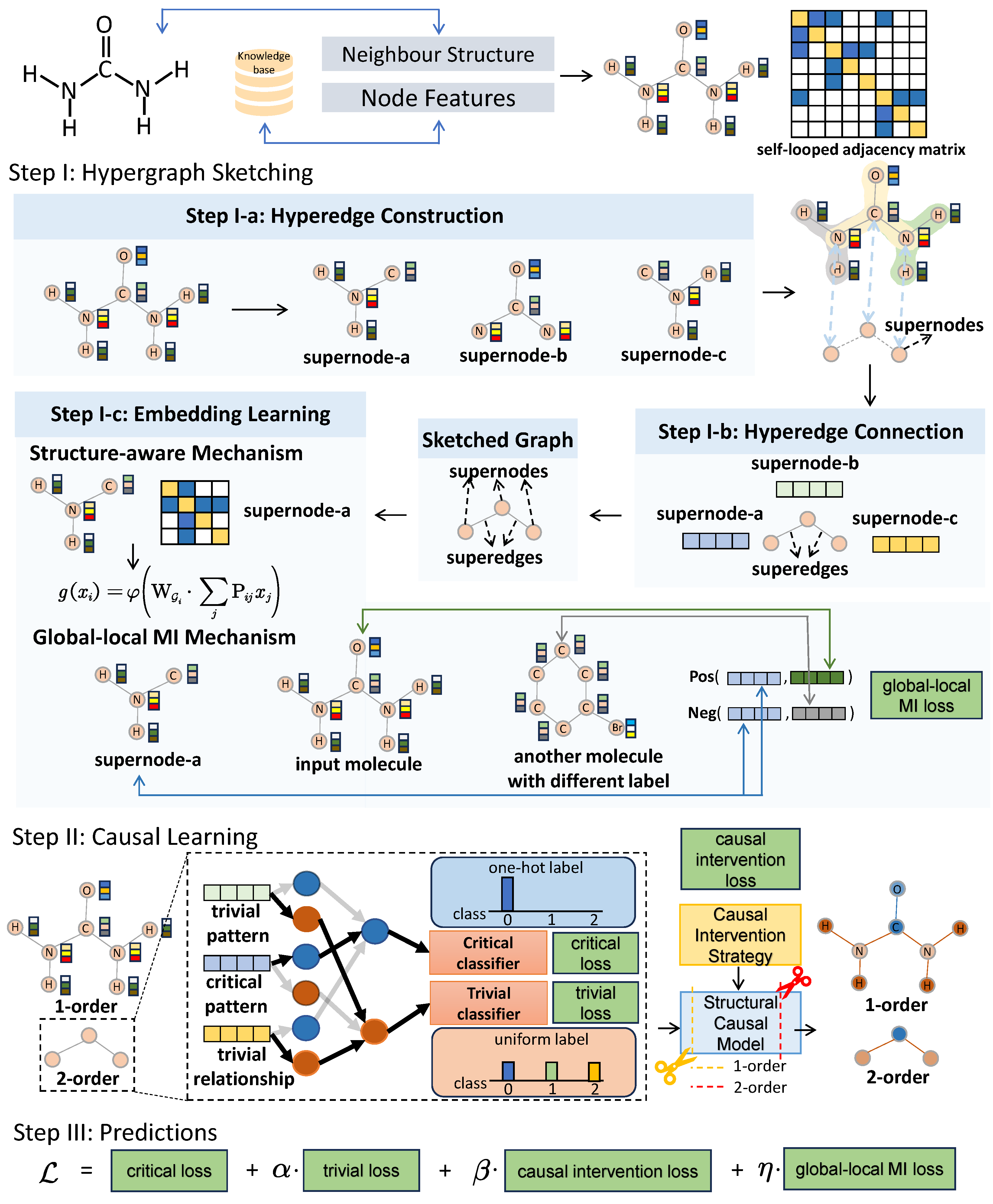
Figure 2.
Structural causal model in HSCGL, herein, overall relationships represent all relationships between patterns in a molecule.
Figure 2.
Structural causal model in HSCGL, herein, overall relationships represent all relationships between patterns in a molecule.
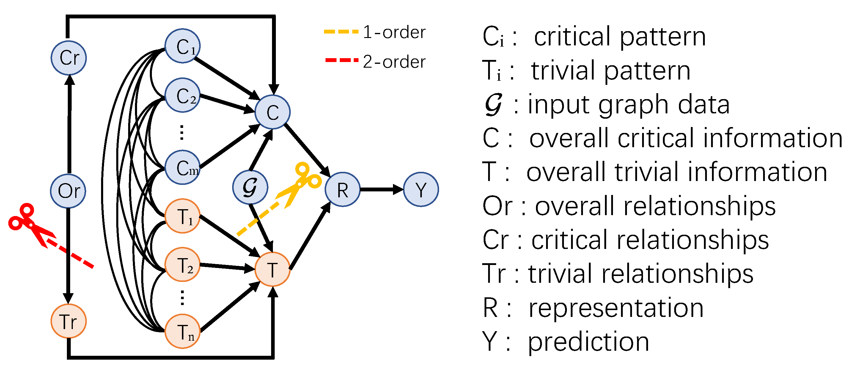
Figure 4.
(a) The performance comparison of different construction methods of superedges in HSCGL; (b) The performance comparison of different components in HSCGL. Dashed lines indicate our HSCGL performance.
Figure 4.
(a) The performance comparison of different construction methods of superedges in HSCGL; (b) The performance comparison of different components in HSCGL. Dashed lines indicate our HSCGL performance.
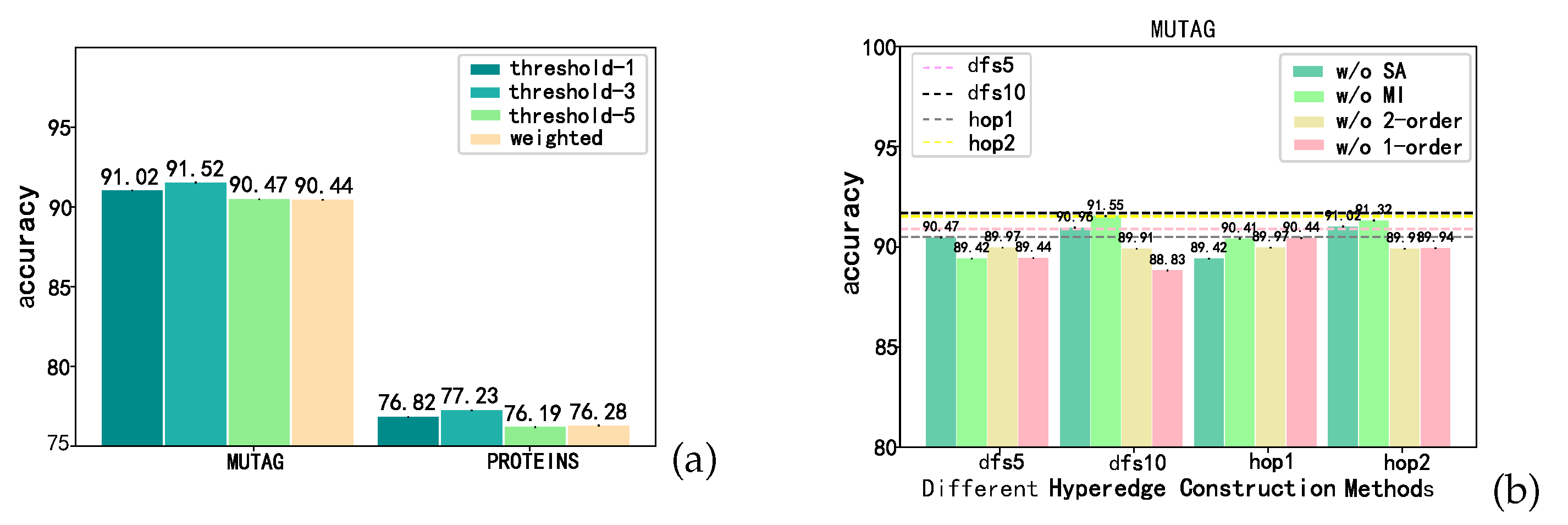
Table 2.
Mean test accuracy (%) of graph classification on the original synthetic dataset and three newly designed synthetic datasets. Our methods are highlighted with a gray. background and the numbers in brackets represent performance degradation than an unbiased dataset.
Table 2.
Mean test accuracy (%) of graph classification on the original synthetic dataset and three newly designed synthetic datasets. Our methods are highlighted with a gray. background and the numbers in brackets represent performance degradation than an unbiased dataset.
| nmi(i) Graph classification on original synthetic dataset with different bias rates b (SYN-b) | |||||
| SYN-0.1 | SYN-0.3 | Unbiased | SYN-0.7 | SYN-0.9 | |
| GCN | 95.44(↓2.61%) | 97.62(↓0.39%) | 98.00 | 96.50(↓1.53%) | 94.75(↓3.32%) |
| 94.69(↓3.26%) | 96.81(↓1.10%) | 97.88 | 97.12(↓0.78%) | 96.75(↓1.15%) | |
| 96.12(↓2.36%) | 98.19(↓0.25%) | 98.44 | 97.50(↓0.95%) | 97.50(↓0.95%) | |
| GAT | 90.31(↓5.81%) | 96.69(↑0.84%) | 95.88 | 94.62(↓1.31%) | 89.56(↓6.59%) |
| 90.94(↓3.89%) | 95.88(↑1.33%) | 94.62 | 94.12(↓0.53%) | 88.62(↓6.34%) | |
| 92.69(↓3.51%) | 97.06(↑1.04%) | 96.06 | 95.38(↓0.71%) | 92.44(↓3.77%) | |
| nmi(ii) Graph classification on synthetic compounded dataset with different bias rates b (SYN-b) | |||||
| SYN-0.1 | SYN-0.3 | Unbiased | SYN-0.7 | SYN-0.9 | |
| GCN | 92.21(↓5.02%) | 95.62(↓1.50%) | 97.08 | 97.33(↑0.26%) | 96.21(↓0.90%) |
| 90.00(↓7.85%) | 96.75(↓0.94%) | 97.67 | 97.46(↓0.22%) | 96.25(↓1.45%) | |
| 96.42(↓1.61%) | 98.17(↑0.17%) | 98.00 | 98.38(↑0.39%) | 97.12(↓0.90%) | |
| GAT | 83.75(↓12.4%) | 92.62(↓3.14%) | 95.62 | 95.54(↓0.08%) | 86.04(↓10.0%) |
| 92.29(↓3.86%) | 96.08(↑0.08%) | 96.00 | 95.42(↓0.60%) | 91.62(↓4.56%) | |
| 94.04(↓3.72%) | 96.38(↓1.32%) | 97.67 | 96.21(↓1.49%) | 95.62(↓1.09%) | |
| nmi(iii) Graph classification on synthetic separated dataset with different bias rates b (SYN-b) | |||||
| SYN-0.1 | SYN-0.3 | Unbiased | SYN-0.7 | SYN-0.9 | |
| GCN | 86.25(↓7.38%) | 91.50(↓1.74%) | 93.12 | 91.88(↓1.33%) | 83.00(↓10.9%) |
| 86.12(↓7.89%) | 90.50(↓3.21%) | 93.50 | 92.25(↓1.34%) | 84.25(↓9.89%) | |
| 90.25(↓5.97%) | 97.12(↑0.90%) | 96.25 | 95.50(↓0.78%) | 89.88(↓6.62%) | |
| GAT | 87.62(↓5.02%) | 90.88(↓1.49%) | 92.25 | 93.00(↑0.81%) | 84.75 (↓8.13%) |
| 88.00(↓8.45%) | 94.50(↓1.69%) | 96.12 | 94.75(↓1.43%) | 83.75(↓12.9%) | |
| 89.88(↓6.86%) | 95.62(↓1.02%) | 96.50 | 95.88(↓0.64%) | 85.25(↓11.7%) | |
| nmi(iv) Graph classification on synthetic biased separated dataset with a fixed rate b = 0.1 | |||||
| nmiand different bias rates (SYN-) | |||||
| SYN-0.1 | SYN-0.3 | Unbiased | SYN-0.7 | SYN-0.9 | |
| GCN | 81.82(↑0.63%) | 72.73(↓10.6%) | 81.31 | 78.48(↓3.48%) | 82.42(↑1.37%) |
| 75.76(↓5.96%) | 82.11(↑1.92%) | 80.56 | 79.39(↓1.45%) | 81.21(↑0.81%) | |
| 83.33(↓4.62%) | 83.82(↓4.06%) | 87.37 | 83.03(↓4.97%) | 83.64(↓4.23%) | |
| GAT | 79.70(↓5.49%) | 83.87(↓0.55%) | 84.33 | 82.85(↓1.76%) | 77.88(↓7.65%) |
| 79.39(↓5.61%) | 80.06(↓4.82%) | 84.11 | 83.64(↓0.56%) | 82.97(↓1.36%) | |
| 81.52(↓4.49%) | 84.75(↓0.70%) | 85.35 | 84.85(↓0.59%) | 85.15(↓0.12%) | |
Table 3.
Ablation study without Causality and without Hypergraph Neural Network (HNN) on three real datasets and one synthetic dataset. "SYN-sep" indicates SYN-0.1 (biased) on synthetic separated datasets.
Table 3.
Ablation study without Causality and without Hypergraph Neural Network (HNN) on three real datasets and one synthetic dataset. "SYN-sep" indicates SYN-0.1 (biased) on synthetic separated datasets.
| w/o Causality | MUTAG | PTC-FR | PTC-FM | SYN-sep |
|---|---|---|---|---|
| hop1 | ||||
| hop2 | ||||
| w/o HNN | MUTAG | PTC-FR | PTC-FM | SYN-sep |
| hop1 | ||||
| hop2 | ||||
| OURS | 91.52 | 69.41 | 68.47 | 90.25 |
Disclaimer/Publisher’s Note: The statements, opinions and data contained in all publications are solely those of the individual author(s) and contributor(s) and not of MDPI and/or the editor(s). MDPI and/or the editor(s) disclaim responsibility for any injury to people or property resulting from any ideas, methods, instructions or products referred to in the content. |
© 2025 by the authors. Licensee MDPI, Basel, Switzerland. This article is an open access article distributed under the terms and conditions of the Creative Commons Attribution (CC BY) license (http://creativecommons.org/licenses/by/4.0/).
Copyright: This open access article is published under a Creative Commons CC BY 4.0 license, which permit the free download, distribution, and reuse, provided that the author and preprint are cited in any reuse.


