Correlating Various Clinical Outcomes Associated with Motor Vehicle Collision-Related Trauma

1. Introduction

Motor vehicles are an integral part of transportation in the United States. Cars, motorcycles, trucks, and scooters are all classified as motor vehicles. With more miles traveled increasing with registered vehicles as the population grows, motor vehicle collisions (MVCs) are a serious concern. Even though MVC fatalities have decreased over the past few years, there has been a 10% increase compared to 2020 [1]. Over the last decade, roadway fatalities have, on average, increased. In 2021, 43,320 people were killed in MCVs, which is the highest number since 2005 [1]. Moreover, MCVs also have financial implications, which include wage and productivity loss, medical expenses, administrative expenses, motor-vehicle property damage, and employer costs. In 2023, these motor-vehicle injury costs were $513.8 billion [2]. Due to these risks, technology such as seatbelts, helmets, and policies such as reducing the blood alcohol concentration (BAC) limit have been implemented.

Helmet use, particularly in bicycle and motorcycle crashes, has been proven to be effective in reducing the severity of head injuries. In a 2016 study, unhelmeted motorcycle and moped riders were nearly three times more likely to die [3]. Lack of helmet use is strongly associated with higher Abbreviated Injury Scale (AIS) scores for head trauma, which measure injury severity from 1 (minor) to 6 (unsurvivable). Higher AIS head scores are predictive of worse outcomes, including long-term disability or death. Overall, helmet use can reduce the risk of head injury by up to 74% in MCVs, and halves the risk of severe traumatic brain injury and death [4-7]. However, the decrease in fatality rates is reduced with the looseness of helmet laws from state to state [8].

Alcohol intoxication is also a major risk factor in MCVs. Elevated BAC has a well-established association with slower reaction times, impaired judgment, and decreased coordination, all of which significantly increase the likelihood of crashes and injury severity.

According to the National Highway Traffic Safety Administration, BAC levels as low as 0.02% can cause drivers to begin to experience altered visual functions, reduced ability to multitask, and some loss of judgment [9]. At a 0.05% BAC, drivers can experience reduced ability to track moving objects, difficulty steering, and, most importantly, a reduced response to emergencies [9]. MCVs that involve patients who test with a BAC above the legal limit sustain a higher injury severity score and mortality than negative patients, and above limit patients are more likely to be found at fault in the crash [10-12]. Interestingly, patients with high BAC levels had increased odds of being unhelmeted, and due to the compounding effect, can be up to 3 times more likely to die than BAC-negative patients [10, 12-14].

In addition to clinical outcomes, the financial and systemic implications of MVCs, as mentioned before, are important and are reflected in hospital payor disposition. Insurance status and discharge destinations can offer insight into broader disparities in healthcare access, long-term support, and socioeconomic burden. However, this remains an area for further research.

Given the established relationships between helmet use, blood alcohol concentration, and injury severity in motor vehicle collisions, further investigation is warranted to expand on how these variables can influence outcomes such as hospital length of stay, injury severity score, and mortality. The primary aim of this study is to provide a comprehensive study on patients involved in MVCs relating to helmet use, BAC, injury severity score, and hospital length of stay. A secondary aim is to analyze ED disposition by a factor of primary payor source. This study can enhance the current understanding of risk factors in trauma care relating to MVCs and contribute to improving outcomes for patients involved in MCVs.

2. Methods

This is a single-center, retrospective review conducted at a Level 1 trauma center in New York City from 1 January 2016 to 31 December 2024. Only patients with motor vehicle injuries were included. Patient data were requested from the trauma registry at our facility (Elmhurst Hospital Center). Our center’s trauma registry utilizes NTRACS software (American College of Surgeons National Trauma Registry System, https://www.facs.org/quality-programs/. Extracted data included demographics, identified based on the cause of injury, helmet use, primary mechanisms (lCD9 or lCDL0 E-Code), trauma type, length of stay (LOS) at the Emergency Department (ED), Intensive care unit (ICU), Hospital (H), the Injury Severity Score (ISS), and the Abbreviated Injury Severity (AIS) head score. When comparing helmet use and blood alcohol concentration (BAC) with the patient’s LOS, ISS, and mortality, the ANOVA method was used, where a p-value of <0.05 was considered significant. LOS and ventilator days with the patient’s ISS, the ANOVA method was used, where a p-value of <0.05 was considered significant. Additionally, data regarding LOS in the ED, ICU, H, trauma type, and type of mortality, means, and percentages were analyzed. For payor type, chi-square tests and Fisher tests were used.

3. Results

During the 9 years, 604 patients were classified as MCVs. Demographic details can be found in Table 1 (Ethnicity/Gender/Count/Percentage of Total Patients/Average Age). The majority of patients were male (74.5%), while females comprised 25.5% of the study population. The average age of all patients was 42.2 years, with females tending to be older on average (49.0 years) compared to males (39.9 years).

In terms of ethnic distribution, the largest group was “Other” (49.5% of males, 12.4% of females), with a significant proportion identifying as Hispanic origin. Among males in “Other”, 35.3% were Hispanic, while 11.6% were non-Hispanic. White patients made up 8.8% of males and 5.6% of females, with an average age of 43.6 years and 53.1 years, respectively. The Asian subgroup accounted for 7.9% of males and 5.0% of females, with older average ages in the female group (56.6 years) compared to males (45.2 years). Black patients represented a smaller portion of the sample, with 3.97% of males and 0.5% of females, averaging 39.9 and 28.8 years, respectively. A minor percentage of patients identified as Native Hawaiian or Other Pacific Islander (0.33% for both males and females), with average ages ranging from 32.5 to 50.7 years.

Figure 1. Count of ED Discharge Patients related to MVCs from 2016 to 2024.

Figure 1. Count of ED Discharge Patients related to MVCs from 2016 to 2024.

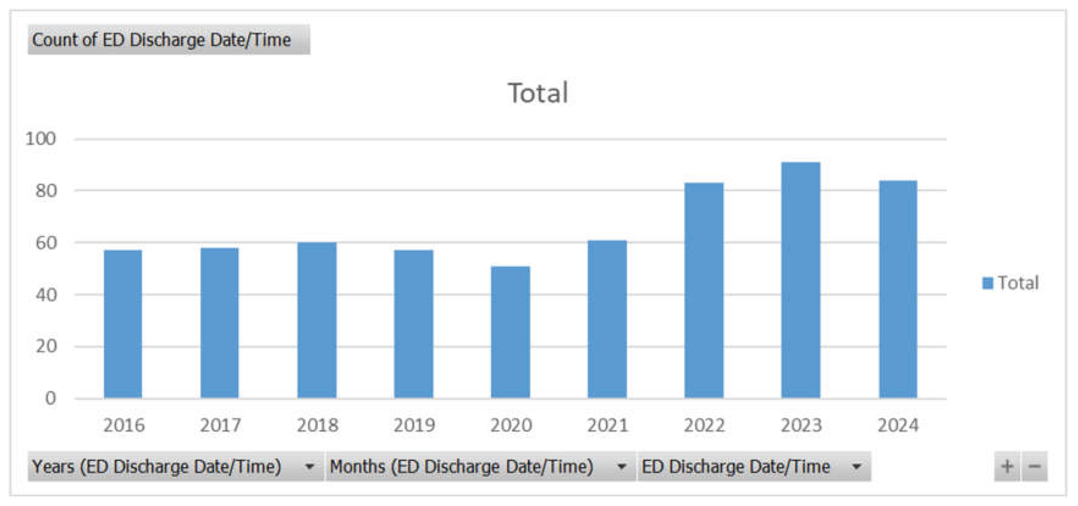
Out of a total of 602 patients, the number of ED discharge patients has increased in the previous years compared to before 2021. There is a drop in ED discharges in 2020, which might suggest the effect COVID had in reducing motor vehicle travel. However, before COVID, ED discharge patients were much less than in the years after COVID. This might suggest a shift in injury severity, practices in the ED, or an increase in vehicle traffic and unsafe motor vehicle travel.

Table 2. This table represents the length of stay in the ED, ICU, and other units in the hospital. The average AIS head score and ISS score are reflected, with a distribution of trauma type.

Hospital Stays	Total	Average	Percentage
Days	7799.00	13.04
Hours	187662.84	104.61	100.00%
ED hours	6295.25	10.53	3.35%
ICU hours	67768.32	113.32	36.11%
Other hours	113599.28	189.97	60.53%
ED/HOSPITAL Initial Gcs Total	6727.00	11.25
Injury Severity Score (ISS)	13505.00	22.58
AIS Head	2217.00	3.71
Trauma Type	598.00		100.00%
Blunt	597.00		99.83%
Penetrating	1.00		0.17%

Table 2. This table represents the length of stay in the ED, ICU, and other units in the hospital. The average AIS head score and ISS score are reflected, with a distribution of trauma type.

Hospital Stays	Total	Average	Percentage
Days	7799.00	13.04
Hours	187662.84	104.61	100.00%
ED hours	6295.25	10.53	3.35%
ICU hours	67768.32	113.32	36.11%
Other hours	113599.28	189.97	60.53%
ED/HOSPITAL Initial Gcs Total	6727.00	11.25
Injury Severity Score (ISS)	13505.00	22.58
AIS Head	2217.00	3.71
Trauma Type	598.00		100.00%
Blunt	597.00		99.83%
Penetrating	1.00		0.17%

Among the cohort, a total of 7,799 hospital days were recorded, with an average length of stay (LOS) of 13.04 days per patient. The majority of time spent in the hospital was distributed as follows: 60.53% in other inpatient units (113,599.28 hours), 36.11% in the ICU (67,768.32 hours), and only 3.35% in the Emergency Department (ED) (6,295.25 hours). This suggests that most patients required prolonged care beyond the ED, with a substantial portion requiring intensive care services. Patients presented with a total initial Glasgow Coma Scale (GCS) score sum of 6,727, averaging 11.25, indicating a moderately impaired level of consciousness at presentation. The average Injury Severity Score (ISS) was 22.58, consistent with severe trauma. The Abbreviated Injury Scale (AIS) Head score averaged 3.71, indicating that head injuries were common and generally moderate to severe. Out of 598 total trauma cases, 99.83% were blunt trauma, while only 0.17% were penetrating injuries, reflecting the predominance of MVCs and similar blunt-force mechanisms.

Table 3. Patient Mortality and Discharge Disposition following Motor Vehicle Collisions.

Mortality	Count of Patients	Count of Signs of Life
Arrived with NO signs of life	35	5.79%
Died as full code	34	5.63%
Died unknown	1	0.17%
Arrived with signs of life	569	94.21%
blank	1	0.17%
Died after withdrawal of care	13	2.15%
Died as full code	44	7.28%
Died with care, not begun DNR/DNI	6	0.99%
Discharged to Home or Self-care (Routine Discharge)	308	50.99%
Home with services	20	3.31%
Homeless/Shelter	1	0.17%
Hospice	2	0.33%
Inpatient Psych Care	1	0.17%
Inpatient Rehabilitation	33	5.46%
Left AMA	10	1.66%
Met brain death criteria	17	2.81%
New placement at Skilled Nursing Facility	13	2.15%
Other Acute Care Hospital Emergency Department	14	2.32%
Other Acute Care Hospital In-Patient	11	1.82%
Other Health Care Facility	5	0.83%
Police Custody/Jail/Prison	5	0.83%
Spinal Cord Injury Rehabilitation	2	0.33%
Sub-Acute Inpatient Rehabilitation	19	3.15%
Traumatic Brain Rehabilitation	44	7.28%

Table 3. Patient Mortality and Discharge Disposition following Motor Vehicle Collisions.

Mortality	Count of Patients	Count of Signs of Life
Arrived with NO signs of life	35	5.79%
Died as full code	34	5.63%
Died unknown	1	0.17%
Arrived with signs of life	569	94.21%
blank	1	0.17%
Died after withdrawal of care	13	2.15%
Died as full code	44	7.28%
Died with care, not begun DNR/DNI	6	0.99%
Discharged to Home or Self-care (Routine Discharge)	308	50.99%
Home with services	20	3.31%
Homeless/Shelter	1	0.17%
Hospice	2	0.33%
Inpatient Psych Care	1	0.17%
Inpatient Rehabilitation	33	5.46%
Left AMA	10	1.66%
Met brain death criteria	17	2.81%
New placement at Skilled Nursing Facility	13	2.15%
Other Acute Care Hospital Emergency Department	14	2.32%
Other Acute Care Hospital In-Patient	11	1.82%
Other Health Care Facility	5	0.83%
Police Custody/Jail/Prison	5	0.83%
Spinal Cord Injury Rehabilitation	2	0.33%
Sub-Acute Inpatient Rehabilitation	19	3.15%
Traumatic Brain Rehabilitation	44	7.28%

Among the 604 patients included in this analysis, 35 patients (5.79%) arrived at the hospital with no signs of life. Of these, 34 (5.63%) were confirmed deceased as full code, and 1 patient (0.17%) had an unknown cause of death. The majority of patients, 569 (94.21%), arrived with signs of life. Among this group, 63 patients (10.42%) died during hospitalization, with 44 (7.28%) dying as full code, 13 (2.15%) following the withdrawal of care, and 6 (0.99%) categorized as DNR/DNI, where care was not initiated. Seventeen patients (2.81%) met brain death criteria. Regarding discharge disposition, 308 patients (50.99%) were discharged home or to self-care, while 20 (3.31%) required home services. A small number of patients were discharged to alternative facilities or care pathways, including 33 (5.46%) to inpatient rehabilitation, 19 (3.15%) to sub-acute inpatient rehabilitation, and 44 (7.28%) to traumatic brain rehabilitation centers. Additionally, 13 patients (2.15%) were transferred to skilled nursing facilities, 14 (2.32%) to other acute care hospital emergency departments, and 11 (1.82%) to other acute care hospital inpatient units. Smaller proportions of patients were discharged to hospice, inpatient psychiatric care, other healthcare facilities, correctional facilities, or specialized rehabilitation centers. These findings highlight that while the majority of patients survived their injuries, a significant proportion required specialized or prolonged care, and mortality remained notable among those arriving with or without signs of life.

Table 4. Regression Analysis: Helmet Use and Length of Stay.

Regression Statistics
Multiple R	0.02898106
R Square	0.000839902
Adjusted R Square	-0.003032812
Standard Error	12.82906425
Observations	260
ANOVA
	df	SS	MS	F	Significance F
Regression	1	35.69465009	35.69465009	0.216876836	0.641822872
Residual	258	42462.9015	164.5848895
Total	259	42498.59615
	Coefficients	Standard Error	t Stat	P-value	Lower 95%	Upper 95%
Intercept	8.678947368	0.930718143	9.325000741	5.21918E-18	6.846175912	10.51171882
Helmet	0.835338346	1.793724887	0.465700371	0.641822872	-2.696867187	4.367543879

Table 4. Regression Analysis: Helmet Use and Length of Stay.

Regression Statistics
Multiple R	0.02898106
R Square	0.000839902
Adjusted R Square	-0.003032812
Standard Error	12.82906425
Observations	260
ANOVA
	df	SS	MS	F	Significance F
Regression	1	35.69465009	35.69465009	0.216876836	0.641822872
Residual	258	42462.9015	164.5848895
Total	259	42498.59615
	Coefficients	Standard Error	t Stat	P-value	Lower 95%	Upper 95%
Intercept	8.678947368	0.930718143	9.325000741	5.21918E-18	6.846175912	10.51171882
Helmet	0.835338346	1.793724887	0.465700371	0.641822872	-2.696867187	4.367543879

A linear regression analysis was conducted to examine the relationship between helmet use and the outcome of interest across 260 observations. The model demonstrated a very low R-squared value of 0.00084, indicating that helmet use accounted for less than 1% of the variance in the length of stay. The overall regression model was not statistically significant, F(1, 258) = 0.217, p = 0.642. The coefficient for helmet use was 0.84 (p = 0.642), with a 95% confidence interval ranging from -2.70 to 4.37, suggesting no significant association between helmet use and the length of stay measured. The intercept was significant at 8.68 (p < 0.001), indicating the estimated length of stay when helmet use is absent. These findings suggest that helmet use, within this sample, did not significantly impact the measured outcome.

Table 5. Regression Analysis: Helmet Use and Injury Severity Score.

Regression Statistics
Multiple R	0.084340862
R Square	0.007113381
Adjusted R Square	0.003279842
Standard Error	12.50303003
Observations	261
ANOVA
	df	SS	MS	F	Significance F
Regression	1	290.0726135	290.0726135	1.85556503	0.174321005
Residual	259	40488.37183	156.32576
Total	260	40778.44444
	Coefficients	Standard Error	t Stat	P-value	Lower 95%	Upper 95%
Intercept	19.8	0.907065134	21.82864191	1.22713E-60	18.01383858	21.58616142
Helmet	2.369014085	1.739120014	1.36219126	0.174321005	-1.055601146	5.793629315

Table 5. Regression Analysis: Helmet Use and Injury Severity Score.

Regression Statistics
Multiple R	0.084340862
R Square	0.007113381
Adjusted R Square	0.003279842
Standard Error	12.50303003
Observations	261
ANOVA
	df	SS	MS	F	Significance F
Regression	1	290.0726135	290.0726135	1.85556503	0.174321005
Residual	259	40488.37183	156.32576
Total	260	40778.44444
	Coefficients	Standard Error	t Stat	P-value	Lower 95%	Upper 95%
Intercept	19.8	0.907065134	21.82864191	1.22713E-60	18.01383858	21.58616142
Helmet	2.369014085	1.739120014	1.36219126	0.174321005	-1.055601146	5.793629315

A linear regression analysis was conducted to evaluate the relationship between helmet use and Injury Severity Score (ISS) among 261 patients. The model produced a low R² value of 0.0071, indicating that helmet use explained less than 1% of the variance in ISS. The overall regression was not statistically significant, F(1, 259) = 1.86, p = 0.17. The regression coefficient for helmet use was 2.37 (SE = 1.74), suggesting that helmet use was associated with an estimated increase of 2.37 points in ISS; however, this effect was not statistically significant (p = 0.17). The 95% confidence interval for the helmet coefficient ranged from -1.06 to 5.79, crossing zero, further indicating no reliable effect. The intercept was 19.80 (SE = 0.91, p < .001), representing the expected ISS when helmet use was absent. These results suggest that, within this sample, helmet use was not a significant predictor of injury severity as measured by ISS.

Table 6. Regression Analysis: Helmet Use and Mortality.

Regression Statistics
Multiple R	0.041703506
R Square	0.001739182
Adjusted R Square	-0.002115106
Standard Error	0.324486507
Observations	261
ANOVA
	df	SS	MS	F	Significance F
Regression	1	0.047510999	0.047510999	0.451233023	0.502348714
Residual	259	27.27049666	0.105291493
Total	260	27.31800766
	Coefficients	Standard Error	t Stat	P-value	Lower 95%	Upper 95%
Intercept	0.110526316	0.023540725	4.695110874	4.32421E-06	0.06417073	0.156881901
Helmet	0.030318755	0.045134737	0.671738806	0.502348714	-0.058559016	0.119196525

Table 6. Regression Analysis: Helmet Use and Mortality.

Regression Statistics
Multiple R	0.041703506
R Square	0.001739182
Adjusted R Square	-0.002115106
Standard Error	0.324486507
Observations	261
ANOVA
	df	SS	MS	F	Significance F
Regression	1	0.047510999	0.047510999	0.451233023	0.502348714
Residual	259	27.27049666	0.105291493
Total	260	27.31800766
	Coefficients	Standard Error	t Stat	P-value	Lower 95%	Upper 95%
Intercept	0.110526316	0.023540725	4.695110874	4.32421E-06	0.06417073	0.156881901
Helmet	0.030318755	0.045134737	0.671738806	0.502348714	-0.058559016	0.119196525

A linear regression analysis was performed to examine the relationship between helmet use and mortality in motor vehicle crashes. The model explained very little of the variance in mortality (R² = 0.0017), with an adjusted R² of -0.0021, indicating that helmet use was not a meaningful predictor of mortality in this sample of 261 observations. The overall regression was not statistically significant (F(1, 259) = 0.45, p = 0.50). The coefficient for helmet use was positive but not significant (β = 0.03, SE = 0.045, t = 0.67, p = 0.50), suggesting no evidence of an association between helmet use and mortality after controlling for the intercept. The intercept was significant (β = 0.11, p < 0.001), representing the baseline mortality level when helmet use is absent.

Table 7. Regression Analysis: Blood Alcohol Concentration and Injury Severity Score.

Regression Statistics
Multiple R	0.014229126
R Square	0.000202468
Adjusted R Square	-0.001805158
Standard Error	10.97887658
Observations	500
ANOVA
	df	SS	MS	F	Significance F
Regression	1	12.15596746	12.15596746	0.100849494	0.750945686
Residual	498	60026.79403	120.535731
Total	499	60038.95
	Coefficients	Standard Error	t Stat	P-value	Lower 95%	Upper 95%
Intercept	21.38403956	0.593634461	36.02223414	8.6128E-141	20.21770279	22.55037632
ETOH Level	0.001388116	0.004371081	0.317568093	0.750945686	-0.007199918	0.00997615

Table 7. Regression Analysis: Blood Alcohol Concentration and Injury Severity Score.

Regression Statistics
Multiple R	0.014229126
R Square	0.000202468
Adjusted R Square	-0.001805158
Standard Error	10.97887658
Observations	500
ANOVA
	df	SS	MS	F	Significance F
Regression	1	12.15596746	12.15596746	0.100849494	0.750945686
Residual	498	60026.79403	120.535731
Total	499	60038.95
	Coefficients	Standard Error	t Stat	P-value	Lower 95%	Upper 95%
Intercept	21.38403956	0.593634461	36.02223414	8.6128E-141	20.21770279	22.55037632
ETOH Level	0.001388116	0.004371081	0.317568093	0.750945686	-0.007199918	0.00997615

A linear regression was conducted to assess the association between ETOH Level and Injury Severity Score (ISS) in 500 cases. The model explained a negligible amount of variance in ISS (R² = 0.0002), with an adjusted R² of -0.0018, indicating that ETOH level did not meaningfully predict injury severity. The overall regression was not statistically significant (F(1, 498) = 0.10, p = 0.75). The coefficient for ETOH level was positive but not statistically significant (β = 0.0014, SE = 0.0044, t = 0.32, p = 0.75), suggesting no evidence of an association between ETOH level and injury severity in this sample. The intercept was significant (β = 21.38, p < 0.001), representing the average injury severity score when ETOH level is zero. In conclusion, ETOH level was not a significant predictor of injury severity in this dataset.

Table 8. Regression Analysis: ETOH Level and Hospital Length of Stay.

Regression Statistics
Multiple R	0.051681003
R Square	0.002670926
Adjusted R Square	0.000660182
Standard Error	27.05380799
Observations	498
ANOVA
	df	SS	MS	F	Significance F
Regression	1	972.2139861	972.2139861	1.328327175	0.249658193
Residual	496	363026.6294	731.908527
Total	497	363998.8434
	Coefficients	Standard Error	t Stat	P-value	Lower 95%	Upper 95%
Intercept	15.89969566	1.464958994	10.85333837	9.08876E-25	13.02140534	18.77798598
ETOH Level	-0.012445909	0.010798765	-1.15253077	0.249658193	-0.033662872	0.008771054

Table 8. Regression Analysis: ETOH Level and Hospital Length of Stay.

Regression Statistics
Multiple R	0.051681003
R Square	0.002670926
Adjusted R Square	0.000660182
Standard Error	27.05380799
Observations	498
ANOVA
	df	SS	MS	F	Significance F
Regression	1	972.2139861	972.2139861	1.328327175	0.249658193
Residual	496	363026.6294	731.908527
Total	497	363998.8434
	Coefficients	Standard Error	t Stat	P-value	Lower 95%	Upper 95%
Intercept	15.89969566	1.464958994	10.85333837	9.08876E-25	13.02140534	18.77798598
ETOH Level	-0.012445909	0.010798765	-1.15253077	0.249658193	-0.033662872	0.008771054

A linear regression analysis was conducted to evaluate the relationship between ETOH level and hospital length of stay (LOS) in 498 patients. The model explained a very small portion of the variance in LOS (R² = 0.0027), with an adjusted R² of 0.0007, suggesting minimal explanatory power. The regression model was not statistically significant (F(1, 496) = 1.33, p = 0.25). The coefficient for ETOH level was negative but not statistically significant (β = -0.012, SE = 0.011, t = -1.15, p = 0.25), indicating no meaningful association between ETOH level and hospital LOS. The intercept was statistically significant (β = 15.90, p < 0.001), representing the expected LOS when ETOH level is zero. In summary, ETOH level was not a significant predictor of hospital length of stay in this dataset.

Table 9. Regression Analysis: ETOH Level and Mortality.

Regression Statistics
Multiple R	0.027908509
R Square	0.000778885
Adjusted R Square	-0.00123162
Standard Error	0.334916813
Observations	499
ANOVA
	df	SS	MS	F	Significance F
Regression	1	0.043455219	0.043455219	0.387407518	0.533950731
Residual	497	55.74812795	0.112169272
Total	498	55.79158317
	Coefficients	Standard Error	t Stat	P-value	Lower 95%	Upper 95%
Intercept	0.12193493	0.018109157	6.733330088	4.59084E-11	0.086354989	0.15751487
ETOH Level	8.317E-05	0.000133623	0.622420692	0.533950731	-0.000179366	0.000345706

Table 9. Regression Analysis: ETOH Level and Mortality.

Regression Statistics
Multiple R	0.027908509
R Square	0.000778885
Adjusted R Square	-0.00123162
Standard Error	0.334916813
Observations	499
ANOVA
	df	SS	MS	F	Significance F
Regression	1	0.043455219	0.043455219	0.387407518	0.533950731
Residual	497	55.74812795	0.112169272
Total	498	55.79158317
	Coefficients	Standard Error	t Stat	P-value	Lower 95%	Upper 95%
Intercept	0.12193493	0.018109157	6.733330088	4.59084E-11	0.086354989	0.15751487
ETOH Level	8.317E-05	0.000133623	0.622420692	0.533950731	-0.000179366	0.000345706

A linear regression analysis was performed to examine the relationship between ETOH level and the outcome variable in a sample of 499 observations. The model accounted for a negligible portion of the variance (R² = 0.0008), with an adjusted R² of -0.0012, indicating no meaningful predictive power. The regression was not statistically significant (F(1, 497) = 0.39, p = 0.53). The coefficient for ETOH level was extremely small and not statistically significant (β = 0.000083, SE = 0.000134, t = 0.62, p = 0.53), suggesting no association between ETOH level and the outcome. The intercept was statistically significant (β = 0.122, p < 0.001), representing the expected value of the outcome when ETOH level is zero. In conclusion, ETOH level was not a significant predictor of the outcome in this dataset.

Table 10. Table of Primary Payor Source by ED Disposition.

Table of Primary Payor Source by ED Disposition													Table of Primary Payor Source by ED Disposition
Primary Payor Source(Primary Payor Source)	ED Disposition(ED Disposition)
	Admitted	Died in ED		Died on Arrival	Died within 15 minutes	Discharged to Home or Self-care (Routine Discharge)			Not Applicable	Transferred to Another Hospital Emergency Dept.		Total
	1	0		0	0	0			0	0		.
unk	7	5		4	2	0			0	4		22
Auto	16	0		0	0	0			0	0		16
Blue Cross	11	0		1	0	0			0	0		12
Commercial	97	0		1	1	1			0	4		104
Corrections	2	0		0	0	0			0	0		2
HMO	1	0		0	0	0			0	0		1
Managed Care	4	0		0	0	0			0	0		4
Medicaid	150	2		5	0	3			0	1		161
Medicare	26	2		1	0	0			0	0		29
No Fault	104	0		2	1	1			0	3		111
None	43	3		5	2	2			1	0		56
Other Govmt	3	0		0	0	0			0	0		3
Other	40	5		1	4	1			0	1		52
Self Pay	16	3		3	0	0			0	1		23
Workers Comp	7	0		0	0	0			0	0		7
Total	527	20		23	10	8			1	14		603
Frequency Missing = 1
Statistic			DF					Value			Prob
WARNING: 88% of the cells have expected counts less
Than 5. Chi-Square may not be a valid test.
Chi-Square			84					158.9329			<.0001
Likelihood Ratio Chi-Square			84					124.8594			0.0026
Mantel-Haenszel Chi-Square			1					1.0929			0.2958
Phi Coefficient								0.5134
Contingency Coefficient								0.4567
Cramer's V								0.2096
Fisher's Exact Test
Table Probability (P)							<.0001
Monte Carlo Estimate for the Exact Test
Pr <= P							<.0001
99% Lower Conf Limit							<.0001
99% Upper Conf Limit							0.0005
Number of Samples							10000
Initial Seed							610796875

Table 10. Table of Primary Payor Source by ED Disposition.

Table of Primary Payor Source by ED Disposition													Table of Primary Payor Source by ED Disposition
Primary Payor Source(Primary Payor Source)	ED Disposition(ED Disposition)
	Admitted	Died in ED		Died on Arrival	Died within 15 minutes	Discharged to Home or Self-care (Routine Discharge)			Not Applicable	Transferred to Another Hospital Emergency Dept.		Total
	1	0		0	0	0			0	0		.
unk	7	5		4	2	0			0	4		22
Auto	16	0		0	0	0			0	0		16
Blue Cross	11	0		1	0	0			0	0		12
Commercial	97	0		1	1	1			0	4		104
Corrections	2	0		0	0	0			0	0		2
HMO	1	0		0	0	0			0	0		1
Managed Care	4	0		0	0	0			0	0		4
Medicaid	150	2		5	0	3			0	1		161
Medicare	26	2		1	0	0			0	0		29
No Fault	104	0		2	1	1			0	3		111
None	43	3		5	2	2			1	0		56
Other Govmt	3	0		0	0	0			0	0		3
Other	40	5		1	4	1			0	1		52
Self Pay	16	3		3	0	0			0	1		23
Workers Comp	7	0		0	0	0			0	0		7
Total	527	20		23	10	8			1	14		603
Frequency Missing = 1
Statistic			DF					Value			Prob
WARNING: 88% of the cells have expected counts less
Than 5. Chi-Square may not be a valid test.
Chi-Square			84					158.9329			<.0001
Likelihood Ratio Chi-Square			84					124.8594			0.0026
Mantel-Haenszel Chi-Square			1					1.0929			0.2958
Phi Coefficient								0.5134
Contingency Coefficient								0.4567
Cramer's V								0.2096
Fisher's Exact Test
Table Probability (P)							<.0001
Monte Carlo Estimate for the Exact Test
Pr <= P							<.0001
99% Lower Conf Limit							<.0001
99% Upper Conf Limit							0.0005
Number of Samples							10000
Initial Seed							610796875

A contingency analysis was performed to examine the association between Primary Payor Source and Emergency Department (ED) Disposition in 603 patients. The overall relationship between payor source and ED disposition was found to be statistically significant. The chi-square test revealed a significant association between payor type and ED disposition (χ²(84) = 158.93, p < .0001). However, 88% of the cells had expected counts less than 5, indicating that the assumptions for the chi-square test were not fully met. To account for this, Fisher’s Exact Test using Monte Carlo simulation was conducted, which also showed a statistically significant association (p < .0001, 99% CI: <.0001 to 0.0005). The strength of association was small to moderate, as reflected by Cramer's V = 0.21. These findings suggest that a patient's primary payor source is significantly associated with their ED disposition, though the strength of this association is limited.

4. Discussion

This study provides valuable insight into the MCVs over 9 years, focusing on the demographics, ED disposition, length of stay, helmet use effectiveness, BACs, and payor disposition. Similar to other study cohorts, there was a predominantly male population with an average age in the 30s and early 40s [3-6, 15, 16]. Our cohort had a notable proportion of patients identifying as Hispanic. This could be a representation of the community that Elmhurst Hospital is located in, and may not be generalized to other populations. Additionally, similar to the data from the U.S. Department of Transportation, there was a peak of fatalities, thus ED admits and discharges, in 2021, and this number has been decreasing; however, it is still above the number before 2020 [1]. This could reflect a negative shift in motor vehicle practices and safety after COVID.

Our cohort had an average hospital length of stay (LOS) of 13.04 days, with most time spent in inpatient and ICU settings. This LOS is longer than some published averages, such as 3.1 days reported in another trauma cohort, though differences in injury severity and trauma system resources may explain this difference [17]. Studies consistently show that higher injury severity scores (ISS) and more severe injuries (e.g., ISS ≥12 or LOS ≥7 days) are associated with longer hospital stays and poorer long-term outcomes [5, 18, 19]. In particular, patients with severe injuries (ISS >= 12) have significantly longer LOS and worse physical health at 12 months post-injury [18]. Our data of ISS = 22.6 aligns with the findings, thus supporting that injury severity positively correlates with prolonged hospitalization [18]. However, there is limited research that delves into ED length of stay and ICU length of stay. Our cohort also had an AIS head score of 3.71, indicating a predominance of moderate to severe head injuries. However, we did not delve into the consequences of this score. However, literature does indicate that higher AIS head scores are strongly associated with increased mortality and a greater likelihood of discharge to rehabilitation [20]. Furthermore, AIS scores > 2 have been found to have a link to non-helmeted groups, which could indicate that a majority of our population did not have helmets [5]. Our cohort does model the consensus that blunt trauma accounts for nearly all cases in MVCs [17].

Helmeted individuals in our dataset appeared to have shorter hospital stays and lower mortality rates compared to unhelmeted individuals, suggesting a potential protective effect. However, the regression analyses for helmet use found no statistically significant association between helmet use and length of stay, injury severity score, or mortality. This contrasts with most research that shows that helmet use is strongly associated with lower mortality and short hospital stays [5, 8, 18, 19]. For example, helmet use has been linked to a 56% decrease in mortality and an 8% reduction in hospital charges, and universal helmet laws are associated with a 36–45% decline in motorcycle crash mortality [8, 19]. However, some studies indicate that helmet type might not be a predictor of injury severity, and the protective effect of helmets may be less pronounced in certain groups and settings [16]. The null findings may reflect sample size, local helmet compliance, or helmet quality used.

The regression analyses for BAC also found no significant association between BAC and injury severity, length of stay, or mortality. Previous research indicates that alcohol intoxication increases the risk of severe injury and death, and is also associated with helmet non-use [12, 20, 21, 22]. In Wiratama et al., alcohol-involved riders were 9.47 times more likely to sustain fatal injuries, and alcohol-involved and unhelmeted riders were 18 times more likely [20]. This indicates the dangerous nature of alcohol and MVCs; however, Li et al. have indicated that alcohol intoxication had a high risk for mortality but was not statistically significant in their cohort [4]. This suggests that other factors, such as injury mechanism and hospital care, may mediate outcomes. Additionally, our observed mortality rate (5.8% on arrival with no signs of life) is consistent with other studies, where mortality rates range from 5% to 12% [4, 16].

However, our study did find a statistically significant association between payor source and ED disposition, though the strength was modest. The literature on payor status and trauma outcomes is limited, but differences in access to care and discharge disposition by insurance type have been suggested as potential contributors to disparities in trauma outcomes [15].

4.1. Strengths

This study provides a comprehensive, multi-faceted analysis of MVCs over 9 years at a major urban trauma center, with a focus on injury severity, hospital and ICU length of stay (LOS), helmet use, blood alcohol concentration (BAC), and primary payor status. This study adds valuable insight into payor type by ED Disposition, an area that is underrepresented in current trauma literature. The inclusion of variables such as ISS and LOS allows for a more nuanced understanding of hospital resource utilization. The alignment of our ISS and LOS data with previously published findings also supports the internal validity of the dataset. Moreover, our sample reflects the trauma burden at Elmhurst Hospital, a high proportion of Hispanic and underinsured patients.

4.2. Limitations

Despite its strengths, this study has limitations. Most notably, many of the regression models yielded non-significant p-values and very low R² values, indicating that the independent variables studied (helmet use, BAC) explained very little of the variability in trauma outcomes. This may be due to confounding variables not accounted for in the model, insufficient sample sizes within subgroups, or how variables were categorized. For example, BAC was treated as a continuous variable, instead of analyzing BAC in categorical ranges (e.g., 0, 0.01–0.08, >0.08), which may have revealed significant relationships. Similarly, there is a lack of interaction analysis between BAC and helmet use, despite prior research indicating that there might be a compounding effect. Additionally, the cohort largely reflects the demographic profile of the community surrounding Elmhurst Hospital, with a significant proportion identifying as Hispanic. While this provides important insight into local trends, it may not be representative of trauma populations in other geographic or demographic contexts. Additionally, while the analysis captured overall LOS, ICU LOS, and ED disposition, it did not examine the consequences of high AIS scores. The quality and type of helmets used would have been beneficial to add to the dataset.

5. Conclusion

This study provides a comprehensive 9-year overview of MVC trauma care at a Level 1 trauma center in New York City, highlighting patterns in demographics, injury severity, hospital length of stay, helmet use, BAC, and primary payor disposition. Consistent with prior research, the cohort was predominantly male and middle-aged, with a substantial proportion identifying as Hispanic, likely reflecting the community. While helmeted individuals appeared to experience better outcomes, including lower mortality and shorter hospital stays, these associations did not reach statistical significance. Similarly, BAC levels showed no significant correlation with injury severity or outcomes, challenging assumptions about alcohol-related trauma. These null findings may be due to limited sample sizes, data categorization, or unmeasured variables such as helmet quality or injury mechanism. Most importantly, the study found a statistically significant association between primary payor type and emergency department disposition, signaling potential disparities in trauma outcomes that could indicate further research. This study not only reflects local trauma care trends but also contributes to broader discussions on public health, safety policies, and healthcare equity in urban trauma systems.

References

- U.S. Department of Transportation. (2023, February 2). The Roadway Safety Problem | US Department of Transportation. Www.transportation.gov. https://www.transportation.gov/NRSS/SafetyProblem.
- National Safety Council. (2017). Introduction - Injury Facts. Injury Facts. https://injuryfacts.nsc.org/motorvehicle/overview/introduction/.
- Galanis, D.J.; Castel, N.A.; Wong, L.L.; Steinemann, S. Impact of Helmet Use on Injury and Financial Burden of Motorcycle and Moped Crashes in Hawai'i: Analysis of a Linked Statewide Database. Hawai'i J. Med. Public Health: A J. Asia Pac. Med. Public Health 2016, 75, 379–385. [Google Scholar]
- Li, Y.M.; Hu, S.C.; Fu, C.C. Mortality from Motor Vehicle Crash Injuries in Eastern Taiwan 5-year Follow-Up Study. 慈濟醫學雜誌 2006, 18, 23–28. [Google Scholar] [CrossRef] [PubMed]
- Khor, D.; Inaba, K.; Aiolfi, A.; Delapena, S.; Benjamin, E.; Matsushima, K.; Strumwasser, A.M.; & Demetriades, D.; Demetriades, D. The impact of helmet use on outcomes after a motorcycle crash. Injury 2017, 48, 1093–1097. [Google Scholar] [CrossRef] [PubMed]
- Gupta, S.; Klaric, K.; Sam, N.; Din, V.; Juschkewitz, T.; Iv, V.; Park, K.B. Impact of helmet use on traumatic brain injury from road traffic accidents in Cambodia. Traffic Inj. Prev. 2017, 19, 66–70. [Google Scholar] [CrossRef] [PubMed]
- Bambach, M.R.; Mitchell, R.J.; Grzebieta, R.H.; Olivier, J. The effectiveness of helmets in bicycle collisions with motor vehicles: a case-control study. Accid. Anal. Prev. 2013, 53, 78–88. [Google Scholar] [CrossRef] [PubMed]
- Notrica, D.M.; Sayrs, L.W.; Krishna, N.; Davenport, K.P.; Jamshidi, R.; McMahon, L. Impact of helmet laws on motorcycle crash mortality rates. J. Trauma Acute Care Surg. 2020, 89, 962–970. [Google Scholar] [CrossRef] [PubMed]
- Drinking and Driving. (n.d.). Www.dmv.virginia.gov. https://www.dmv.virginia.gov/safety/programs/drinking/drinking-driving.
- Sarmiento, J.M.; Gogineni, A.; Bernstein, J.N.; Lee, C.; Lineen, E.B.; Pust, G.D.; Byers, P.M. Alcohol/Illicit Substance Use in Fatal Motorcycle Crashes. J. Surg. Res. 2020, 256, 243–250. [Google Scholar] [CrossRef] [PubMed]
- Ahmed, N.; Kuo, Y.H.; Sharma, J.; Kaul, S. Elevated blood alcohol impacts hospital mortality following motorcycle injury: A National Trauma Data Bank analysis. Injury 2020, 51, 91–96. [Google Scholar] [CrossRef] [PubMed]
- Kureshi, N.; Walling, S.; Erdogan, M.; Opra, I.; Green, R.S.; Clarke, D.B. Alcohol is a risk factor for helmet non-use and fatalities in off-road vehicle and motorcycle crashes. Eur. J. Trauma Emerg. Surg. : Off. Publ. Eur. Trauma Soc. 2024, 50, 2073–2079. [Google Scholar] [CrossRef] [PubMed]
- Luna, G.K.; Maier, R.V.; Sowder, L.; Copass, M.K.; & Oreskovich, M.R.; Oreskovich, M. R. The Influence of Ethanol Intoxication on the Outcome of Injured Motorcyclists. J. Trauma 1984, 24, 695–700. [Google Scholar] [CrossRef] [PubMed]
- Borges, G.; Orozco, R.; Pérez-Núñez, R.; et al. Substance use and type of Road Traffic Injury in Mexico City. J Prev. 2024, 45, 323–337. [Google Scholar] [CrossRef] [PubMed]
- Jones, M.D.; Eastes, J.G.; Veljanoski, D.; Chapple, K.M.; Bogert, J.N.; Weinberg, J.A. Burden of motorcyclists without helmets in a state without a universal helmet law: a propensity score analysis. Trauma surgery & acute care open 2020, 5, e000583. [Google Scholar] [CrossRef]
- Porto, G.G.; de Menezes, L.P.; Cavalcante, D.K.F. , de Souza, R.R.L., Carneiro, S.C.A.S., Antunes, A.A. Does Type of Helmet and Alcohol Use Increase Facial Trauma Severity? J. Oral Maxillofac. Surg. : Off. J. Am. Assoc. Oral Maxillofac. Surg. 2020, 78, 797.e1–797.e8. [Google Scholar] [CrossRef] [PubMed]
- Hunain, Waqas Arshad, M. ; Saleem, F.; Sattar, A.; Nadeem, K.; & Abubakar, M. About Morbidity, Mortality, and Hospital Stay, Determine the Predictive Value of Injury Severity Scores in Road Traffic Accidents. Pak. J. Med. Health Sci. 2021, 15, 3414–3416. [Google Scholar] [CrossRef]
- Hung, K.K.C. , Kifley, A.; Brown, K.; Jagnoor, J.; Craig, A.; Gabbe, B.; Derrett, S.; Dinh, M.; Gopinath, B.; Cameron, I.D.; FISH Investigators. Impacts of injury severity on long-term outcomes following motor vehicle crashes. BMC Public Health 2021, 21, 602. [Google Scholar] [CrossRef] [PubMed]
- Stewart, N.; MacConchie, J.G.; Castillo, R.; Thomas, P.G.; Cipolla, J.; & Stawicki, S.P.; Stawicki, S. P. Beyond Mortality: Does Trauma-related Injury Severity Score Predict Complications or Lengths of Stay Using a Large Administrative Dataset? J. Emergencies Trauma Shock 2021, 14, 143–147. [Google Scholar] [CrossRef]
- Hubbard, M.E.; Bin Zahid, A.; Vonderhaar, K.; Freeman, D.; Nygaard, R.M.; Kiragu, A.; Guillaume, D. Prediction of discharge destination after traumatic brain injury in children using the head abbreviated injury scale. Brain Inj. 2019, 33, 643–648. [Google Scholar] [CrossRef] [PubMed]
- Wiratama, B.S.; Chen, P.L.; Ma, S.T.; Chen, Y.H.; Saleh, W.; Lin, H.A.; Pai, C.W. Evaluating the combined effect of alcohol-involved and unhelmeted riding on motorcyclist fatalities in Taiwan. Accid. Anal. Prev. 2020, 143, 105594. [Google Scholar] [CrossRef] [PubMed]
- Lin, M.R.; Kraus, J.F. A review of risk factors and patterns of motorcycle injuries. Accident; analysis and prevention 2009, 41, 710–722. [Google Scholar] [CrossRef] [PubMed]