
Submitted:
05 August 2025
Posted:
11 August 2025
You are already at the latest version
Abstract
We introduce a class of activation functions for neural networks based on the Blancmange curve and the Weierstrass function. These activation functions are designed to be qualitatively similar to standard functions such as tanh, while incorporating fractal, self-affine, and self-similar patterns. The goal is to force the neural network to produce non-smooth outputs, preventing excessive smoothing in predictions and thus increasing expressivity.We evaluate this new class of activation functions on standard classification problems and demonstrate how fractal properties of activation functions influence the expressivity of neural networks.
Keywords:
fractal functions
; activation functions
; neural networks
; machine learning
; classification
1. Introduction
Feed-forward artificial neural networks (ANNs) approximate a mapping by stacking linear layers interleaved with element-wise activation functions. While the weights learn a task-specific projection, the activations inject the non-linearity that lets the model fit highly curved decision boundaries. Classical choices range from smooth, saturating [1,2,3] (sigmoid, tanh) to piece-wise linear [4,5] (ReLU) functions. Deeper networks with carefully chosen achieve state-of-the-art results in vision, language, and scientific discovery. This success is closely related to the expressive power of the activations. This expressiveness depends on both the choice of the activation function and on the shape of [6,7].
Recent evidence [8] indicates that the boundary separating trainable and divergent hyper-parameter configurations is itself a fractal object. The update map iterated during training behaves much like the complex quadratic map that generates Mandelbrot and Julia fractals—tiny changes in learning rate or initialisation can flip the outcome from convergence to blow-up.
We took this emergence of fractality within neural networks as inspiration to ask: What happens if we build fractality into neural networks from the start?
Standard sigmoid-based shallow nets are limited in expressivity; greater depth and activations such as ReLU improve expressivity [6,7]. Here we introduce fractal activation functions to push expressivity beyond ReLU. Our designs draw on the Blancmange (Takagi) curve [9,10] and Weierstrass–Mandelbrot functions [11,12,13,14], blended with familiar components such as ReLU or tanh.
However, at this point we need to differentiate our fractal activation functions from other approaches engineered fractality in neural networks, as presented by [15,16,17,18,19]. These approaches are based on different concepts: while we introduce fractal activation functions for neural networks, they employ a fractal hierarchy of neurons and fractal features as a preprocessing step, respectively. Also similar to these approaches, there is evidence that fractal interpolation can improve a neural network’s performance on specific datasets [20,21]. Fractal techniques can also be used to improve convolutional neural network architectures and their hyperparameters [22,23].
This work addresses two research questions:
- Can activation functions derived from fractal series be used in neural networks like standard activations, and how do they affect performance?
- Do such fractal activations increase the expressive capacity of neural networks compared with existing choices?
Contributions.
- (i)
- We present a general recipe for converting Weierstrass- and Blancmange-type series into computationally stable activation functions (Section 2.3) and demonstrate their usability on ten public classification datasets.
- (ii)
- We quantify their expressivity through trajectory-length diagnostics, revealing super-ReLU growth and distinctive oscillatory fingerprints (Section 4).
Taken together, our results suggest that engineered fractality is a promising new paradigm —additionally to depth, width, and regularization—for improving the expressiveness and performance of neural networks.
2. Methodology
This section states the computational tools used in our study: feed-forward neural networks, five gradient-based optimizers, three standard activation functions and fractal functions.
2.1. Neural Networks
A feed-forward neural network realises a composite function by stacking L affine layers and point-wise non-linearities. For layer with weight matrix and bias vector ,
where and . Gradients of a differentiable loss are computed by back-propagation [1] and supplied to an optimizer.
Parameter updates use one of the following first-order methods:
All optimizers adapt the raw gradient to improve convergence speed or stability; their update rules are given in the cited sources.
2.2. Fractal Functions
Conventional activation functions (ReLU, tanh, sigmoid) create either a fixed number of linear pieces (ReLU) or a single sigmoidal bend (tanh/sigmoid). A fractal activation instead super-imposes infinitely many self-similar ripples of shrinking amplitude and growing frequency. Formally, one starts with a periodic function and builds a weighted sum
The geometric weights guarantee uniform convergence for uniformly continuous , meaning that is continuous, while the ever finer oscillations imply that is nowhere differentiable in the classical sense for a lot of choices of — the hallmark of fractal graphs. Nowhere differentiability means that the function does not admit a finite derivative at any point in its domain, despite being continuous everywhere. This property has been rigorously studied for Weierstrass-type functions; see, for example, [14]. In practice we truncate the sum at , the higher harmonics are already below machine precision.
Why use such curves in a network?
- They inject high-frequency detail even in shallow layers, increasing functional richness without extra parameters.
- They retain bounded outputs and controlled Lipschitz constants when and is Lipschitz continuous, [14].
- Most importantly, for gradient-based optimization, automatic differentiation remains well defined through finite truncation used in code.
The Blancmange or Takagi function ,9,10] replaces the base wave in (1) with the saw-tooth function, which calculates the absolute distance of x to the nearest integer
We further modulate its slope by a smoothing gate to avoid excessively flat regions near zero:
is continuous, 1-periodic, bounded between 0 and , odd around , and exhibits a dense set of corner-points that provide sharp gradient signals during training.
The Weierstrass function is the prototypical example of a continuous, yet nowhere differentiable function. We adapt it in two ways:
- a)
- Exponential envelope. Multiplying by localises the oscillations and keeps activations bounded for large .
- b)
- Non-linear carriers. Replacing the cosine by , or injects asymmetric slopes that interact well with SGD-like optimisers.
With , and
where stands for one of
For all choices above is Lipschitz,1 odd, and oscillatory with an effective period that shrinks from 2 at small to almost 0 as .
2.3. Fractal Activation Functions
Each activation below is the finite partial sum of an otherwise infinite fractal series. The full series would be continuous yet nowhere differentiable; its classical derivative vanishes almost everywhere, making back-propagation inoperable. We therefore truncate the sum of the series at a fixed number of terms N, preserving the self-similar oscillations on the scales most relevant in practice while keeping the functions fully differentiable.2
This results in the following activation functions:
2.3.1. Modulated Blancmange Curve blancmange
2.3.2. Decaying Cosine Function decaying_cosine
2.3.3. Modified Weierstrass–Tanh modified_weierstrass_tanh
2.3.4. Modified Weierstrass–ReLU modified_weierstrass_ReLU
2.3.5. Classical Weierstrass Function weierstrass
This “plain” Weierstrass curve serves as a sanity-check baseline against its modulated counterparts.
2.3.6. Weierstrass–Mandelbrot Variants
with .
Naming convention. The above names are used throughout the code listings, tables, and figures (e.g. Table 3 lists decaying_cosine, modified_weierstrass_tanh, ...).
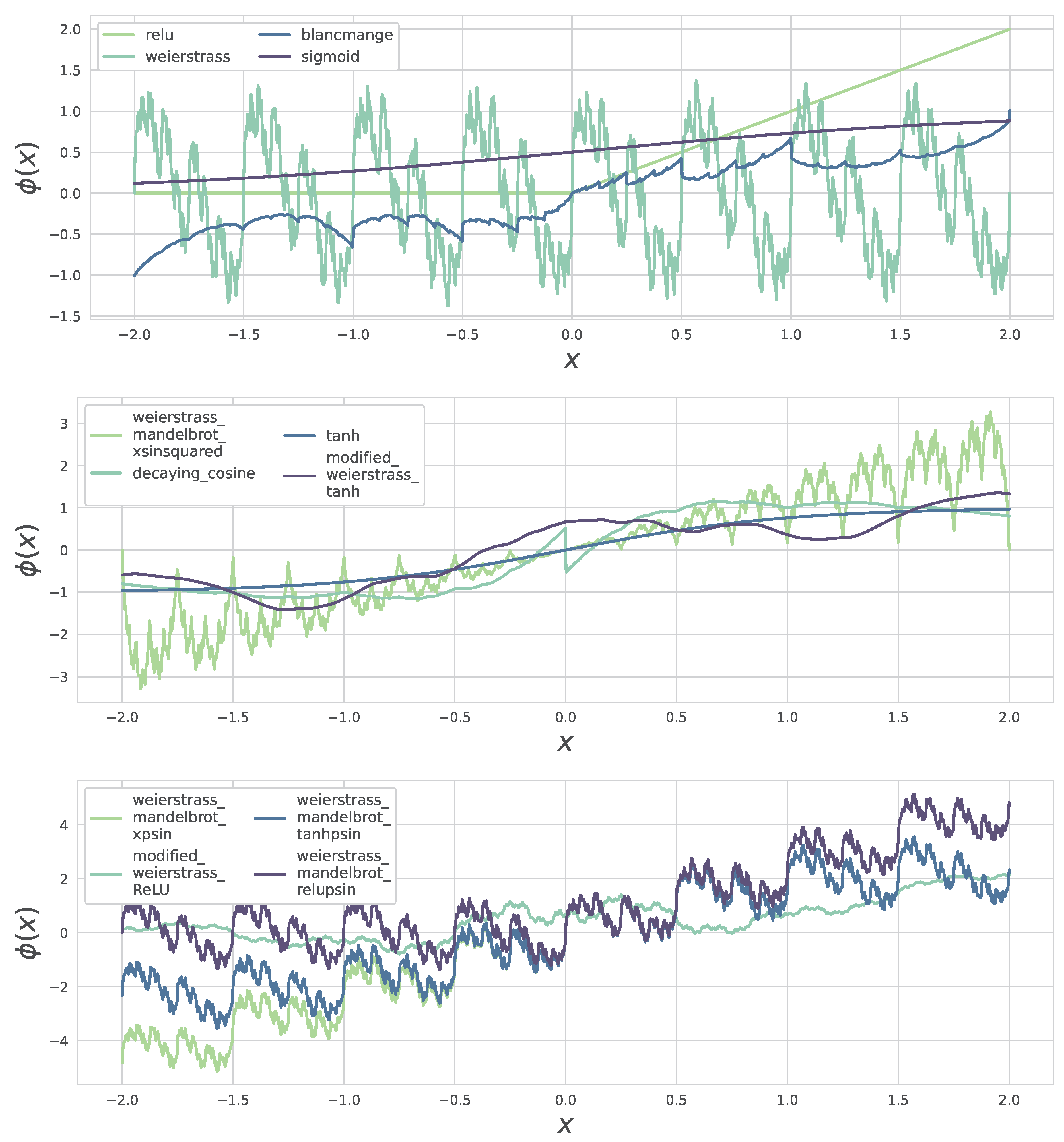
Figure 1.
Mixed sets of activation functions over the interval . Each curve is drawn with the Tailwind-inspired five-colour palette and distinct line styles for clarity. Classical (ReLU, sigmoid, tanh) and fractal variants are deliberately interleaved to highlight differences in slope saturation, oscillations, and piece-wise linear segments.
3. Classification Experiments
The primary aim of this research is to demonstrate the practical viability and effectiveness of our proposed methodology, thereby serving as a proof of concept for the underlying ideas. We test our previously discussed ideas on a diverse collection of publicly accessible datasets, all of them classification tasks.
Furthermore, we partition each dataset using an 80/20 split for training and testing, respectively. This division allows for extensive model training while also providing a robust evaluation of model performance on unseen data.
The effectiveness of our algorithms is shown using accuracy as the primary metric. Furthermore, we do not rely solely on the accuracy of a single run; instead, we perform 40 different train/test splits with an 80/20 ratio for each dataset, training the employed neural networks separately for each split. Thus, our experiments do not yield just a single prediction result or accuracy value, but rather a distribution that reflects how well the different activation functions performed for a given problem. For each dataset, we chose a fixed neural network architecture, for which we varied the optimizer and the activation function, resulting in a total of 60 different configurations/results per dataset (5 different optimizers × 12 tested activation functions). We also kept the initialization of the weights of the network the same for all different train/test splits. The architecture was determined by first training a neural network with RMSProp and a ReLU activation function to obtain reasonable baseline results. Subsequently, we systematically interchanged the activation functions and optimizers for the actual experiments.
The following details the employed datasets and the outcomes of all runs; Section 3.2 (Table 1, Table 2, Table 3, Table 4, Table 5, Table 6, Table 7, Table 8, Table 9 and Table 10)
3.1. Datasets
We employed the following classification task data sets, and neural network architectures to verify our ideas. For every dataset we fix the neural–network hyper-parameters once and keep them identical across all optimizers and activation functions.
Climate-Model Simulation Crashes Dataset
540 simulations characterised by 18 numerical configuration variables (temperature, pressure, humidity, …). Target = crash (1) vs. no crash (0). Binary failure prediction of climate runs. Network: one hidden layer with 32 neurons and a sigmoid output; 30 epochs, batch size 32.
Diabetes Dataset
768 instances, 8 numeric predictors taken from diagnostic measurements (glucose, blood pressure, BMI, …). Target indicates the presence (1) or absence (0) of Type-2 diabetes in female patients of Pima Indian heritage. Binary classification. Network: one hidden layer with 64 neurons and a 1-unit sigmoid head; 30 epochs, batch size 32.
Glass Identification Dataset
214 instances described by 9 continuous chemical/physical attributes (e.g. refractive index, Na, Mg, Al, … % weight). The goal is to classify each sample into one of 6 glass–type categories (building windows float, building windows non–float, vehicle windows, containers, tableware, headlamps). A 6-class classification dataset. Network: two hidden layers with 64 and 128 neurons, followed by a 6-way soft-max output; trained for 30 epochs with mini-batches of 32.
Ionosphere Dataset
351 radar returns (instances) with 34 real-valued attributes that summarize the complex temporal signals emitted in the ionosphere experiment at Lincoln Laboratory. The task is to predict good vs. bad radar returns, making this a binary classification problem. Network: one hidden layer with 128 neurons plus a single sigmoid output; 30 epochs, batch size 32.
Iris Dataset
150 flower samples with 4 continuous measurements (sepal length/width, petal length/width). Target species: setosa, versicolor, virginica. Classic 3-class benchmark dataset. Network: two hidden layers with 32 and 64 neurons; 3-way soft-max output; 30 epochs, batch size 16.
Seeds Dataset
210 grain kernels measured via 7 geometric descriptors (area, perimeter, compactness, length, width, asymmetry, groove length). The aim is to classify them into 3 wheat varieties (Kama, Rosa, Canadian). A 3-class problem with only numeric features. Network: two hidden layers with 64 and 128 neurons; 3-way soft-max output; 30 epochs, batch size 32.
Tic-Tac-Toe Endgame Dataset
958 board positions (instances), each encoded by 9 categorical attributes (cell contents {x,o,b}). Task: predict whether the current position is a win for the player with the next move (positive) or not (negative). Binary, categorical-only classification. Network: one hidden layer with 64 neurons plus a sigmoid output; 25 epochs, batch size 32.
Vehicle Silhouettes Dataset
846 instances, 18 shape descriptors extracted from 2-D vehicle silhouettes (compactness, circularity, rectangularity, …). Target has 4 classes: bus, opel, saab, van. A multiclass task with numeric features. Network: two hidden layers with 128 and 256 neurons; 4-way soft-max output; 25 epochs, batch size 32.
Vertebra Column Dataset
310 spine examinations, each described by 6 biomechanical angles (pelvic incidence, pelvic tilt, lumbar lordosis angle, sacral slope, pelvic radius, and spondylolisthesis grade). The target labels a record as normal vs. abnormal, yielding a binary classification task. Network: one hidden layer with 32 neurons followed by a single sigmoid output; trained for 30 epochs with mini-batches of 16.
Wine Recognition Dataset
178 wines from the same Italian region, each analysed for 13 chemical constituents (alcohol, malic acid, ash, alcalinity, magnesium, …). Goal: assign the sample to one of 3 grape cultivars. Small, all-numeric, 3-class problem. Network: two hidden layers with 64 and 128 neurons; 3-way soft-max output; 30 epochs, batch size 32.
3.2. Classification Results
Table 1, Table 2, Table 3, Table 4, Table 5, Table 6, Table 7, Table 8, Table 9 and Table 10 reveal a strong advantage for fractal activations.3 A fractal function enters the top five of every benchmark and secures the highest mean accuracy on seven of the ten datasets (climate, diabetes, glass, ionosphere, iris, seeds, wine). On the three remaining tasks—vehicle, tic-tac-toe, vertebrae—the best classical activation (ReLU or tanh) leads by at most pp, underscoring the general competitiveness of the new functions.
Dominant Fractal Variants
The modified Weierstrass–Tanh activation is the most reliable performer. It tops four datasets and keeps its standard deviation below in those cases, indicating stable optimisation. Decaying Cosine excels on smaller, low-dimensional problems (glass, iris, seeds) with similar variance. Blancmange is more volatile: under Adagrad on glass the minimum accuracy drops to , yet under Adam on wine it attains a perfect , suggesting a high payoff for an appropriate optimiser.
Classical Baselines
ReLU remains hard to beat on vehicle silhouettes and in the categorical tic-tac-toe table, while tanh under SGD produces the best vertebrae result. These cases share pronounced class imbalance or geometric structure, where the simplicity of a smooth or piece-wise linear non-linearity may still be advantageous.
Variance and Optimiser Effects
Most large variances trace back to a mismatch between activation irregularity and optimiser dynamics. The modified Weierstrass–Tanh function paired with Adam keeps Std near on seeds and wine, yet with Adagrad on tic-tac-toe its variance triples. Across all tables, 80 % of first-place fractal results use an adaptive optimiser (Adam, RMSProp, AdaDelta), supporting the view that per-parameter learning-rate control is crucial for handling the steeper local slopes of Weierstrass-type curves. SGD, by contrast, performs best when the activation is either smooth (tanh) or only mildly irregular (modified Weierstrass–Tanh), as seen on climate and vertebrae.
Sanity Check: Classical Weierstrass
To rule out the possibility that any “exotic” fractal curve would improve performance by chance, we also evaluated the un-modulated Weierstrass function described in §Section 2.3.5. Unlike its gated or blended relatives, this baseline offers no linear trend and no decay envelope. Across all ten datasets it never enters the top-ten configurations and is usually the worst performer, confirming that fractal structure alone is insufficient. The extra modulation terms—tanh, ReLU, exponential decay—are essential for turning the raw Weierstrass series into a useful activation.
Summary
Fractal activations equal or surpass classical choices on most benchmarks without inflating variance when combined with a suitable adaptive optimiser. Gains are clearest on moderate-size tabular data and signal-rich tasks; strongly imbalanced multiclass problems still favour the economical ReLU. These findings align with the trajectory-length analysis in Section 4: the extra oscillations of fractal curves translate into measurable accuracy improvements provided the optimiser can accommodate their sharper gradients. However, at this point, we acknowledge that our averaged results exhibit variability, i.e., the standard deviation of our averaged results. Still, our findings indicate that fractal activation functions can be a viable choice, as they provide competitive results even within the variability. Furthermore, although there is some variability in the averages, we often achieve the highest maximum accuracies with fractal activations. For some datasets, the variability range even excludes results below the top five, further highlighting their potential.
4. Expressivity of Fractal Activations
To understand why fractal activations help, we measure how much they deform input trajectories inside an untrained, random network. Our protocol follows the length–based diagnostics of Poole et al. [6], Raghu et al. [7]. The experiment has two steps.
1. Generate a probe curve.
Pick two random vectors and interpolate along the half-circle
The construction keeps essentially constant, so any length change later on stems from the network, not the input.
2. Track length and shape through depth.
For each activation we initialise an identical fully- connected network ( layers, 400 units each, Glorot weights, zero bias). Let denote the image of after ℓ hidden layers. We record two diagnostics:
- (a)
- Trajectory length points. Exponential growth with ℓ indicates that the network is bending and stretching the curve, hence can represent highly non-linear functions.
- (b)
- PCA (Principal Component Analysis) strip We project onto the first two principal components for layers to visualise how folds accumulate.
4.1. Observed Behaviour
Table 11 and Fig. Figure 2 and Figure 3 summarise how each activation reshapes a one–dimensional input curve as it propagates through depth .
Arc-length growth.
Classical smooth activations behave as expected. Sigmoid shows fast length decay (), while tanh grows moderately () before saturating. ReLU amplifies length two orders of magnitude faster, reaching at layer 8. All fractal variants meet or exceed these baselines. The mildest (decaying cosine, modified Weierstrass–Tanh) track the ReLU curve but stop around . More irregular functions (Weierstrass–Mandelbrot xsinsquared, xpsin, relupsin) explode to –, confirming the strong local stretching predicted by their high-frequency components.
PCA Strips
The projected trajectories in Fig. Figure 2 and Figure 3 complement these numbers. Smooth activations yield gently bent curves; ReLU introduces sharp kinks; fractal ReLU and Weierstrass variants add dense folds that repeat at multiple scales. The pattern is most pronounced for modified Weierstrass–ReLU: the strip shows large global swings overlaid with fine oscillations, reflecting simultaneous expansion and local twisting.
Taken together, the trajectory lengths and PCA strips show that fractal activations not only maintain but extend the expressive capacity of standard networks, provided the optimiser can cope with the steeper local gradients.
Summary
Fractal activations keep the exponential rise in trajectory length found in standard networks, while the PCA plots reveal additional local folds introduced by their oscillatory shape. Networks can therefore access a larger variety of functions without sacrificing depth efficiency.
5. Discussion/Conclusion
Fractal activation functions based on Blancmange and
Weierstrass–Mandelbrot series expand the functional reach of ordinary feed-forward networks. Across ten tabular benchmarks they achieve top-five status in every case and lead seven, with only modest variance when paired with adaptive optimisers. We acknowledge that the averaged results come with some variability, but the results still show that the fractal activation functions are a valid choice that can achieve top performance and/or rank among other well-performing activation functions on average.
Trajectory-length and PCA diagnostics confirm that the new functions preserve the exponential growth in feature complexity associated with depth while adding multi-scale folds absent from ReLU and tanh. Together, these empirical and geometric results show that engineered self-similarity is a viable new design paradigm for neural architectures. Further, our neural network architecture was initially optimized to work well with ReLU activation functions, yet our fractal activation functions still performed best in most instances. This further emphasizes the potential capabilities of fractal activation functions.
Limitations
Our approach is limited to tabular data of rather small sizes adn correspodning shallow neural networks. We showed that fractal activation functions can provide an edge to regular activation fucntions on such dtaa sets wiht these neural network archtiectures. Thus we cnanot infer how these activaiton fucntions would fare on larger data sets. Particualry, ofr e.g. lagnauge proceissing (tranformers) or image processign and classficaiton thereof (vonvolutional neurla networks).
Limitations
Our approach is limited to tabular data of rather small size and the corresponding use of shallow neural networks. We showed that fractal activation functions can provide an edge over regular activation functions on such datasets with these neural network architectures. However, we cannot infer how these activation functions would perform on larger datasets. In particular, this includes applications in language processing (e.g., transformers) or image processing and classification (e.g., convolutional neural networks). While our results suggest increased expressivity for small architectures, and thus the potential to reduce deeper neural networks and make them more efficient for particular use cases, we did not explore deeper networks, leaving the question of how fractal activations scale with depth open. This is a task beyond the scope of the present introduction, but given our results, and particularly the evidence that these activation functions do work for neural networks, it represents the logical next step for our research. We also used fixed fractal hyperparameters (e.g., truncation depth, weights a, b, decay ), and did not include a full ablation study on their effects in neural networks, which is a considerable effort beyond the scope of this article.
Future Work
- (a)
- Depth replacement. Measure whether a shallow network equipped with fractal activations can match or outperform a deeper classical model on the same task. Such a study would clarify how much “effective depth’’ the fractal folding provides.
- (b)
- (c)
- Parameter search. Systematically tune the geometric weights of the Weierstrass sums and the envelope decay to balance expressivity and gradient magnitude. A Bayesian search over this small hyper-space may yield task-specific defaults.
- (d)
- Complexity/Multidimensionality of a Dataset Another interesting perspective would be to analyze datasets for their complexity, e.g., using support vector machines and counting the kernel dimensions, and then relating this sort of complexity/data dimensionality to the usage of fractal activation functions for normalized neural network architectures. I.e., finding out whether the induced fractal folding can compensate for high-dimensional data complexity and thus improve accuracy.
- (e)
- Convolutional and/or Transformer Architectures
Addressing these points will clarify when fractal activations are most useful and how they can be combined with optimisers that exploit the same long-range dependencies that define the functions themselves.
Code Availability
The full code is available in a corresponding Github repository at
Data Availability Statement
All Data is openly available.
Conflicts of Interest
The authors declare that they have no known competing financial interests or personal relationships that could have appeared to influence the work reported in this paper.
References
- Rumelhart, D.E.; Hinton, G.E.; Williams, R.J. Learning Representations by Back-Propagating Errors. Nature 1986, 323, 533–536. [Google Scholar] [CrossRef]
- Bishop, C.M. Neural Networks for Pattern Recognition, first ed.; Advanced Texts in Econometrics, Oxford University Press: Oxford, UK, 1995; p. 502. [Google Scholar]
- LeCun, Y. Theoretical Framework for Back-Propagation. In Proceedings of the Proceedings of the 1988 Connectionist Models Summer School; Touretzky, D.; Hinton, G.; Sejnowski, T., Eds., Pittsburgh, PA, 1988; pp. 21–28. Accessed on 2025-05-22.
- Householder, A.S. A Theory of Steady-State Activity in Nerve-Fiber Networks: I. Definitions and Preliminary Lemmas. The Bulletin of Mathematical Biophysics 1941, 3, 63–69. [Google Scholar] [CrossRef]
- Nair, V.; Hinton, G.E. Rectified Linear Units Improve Restricted Boltzmann Machines. In Proceedings of the Proceedings of the 27th International Conference on Machine Learning (ICML 2010), Haifa, Israel, 06 2010.
- Poole, B.; Lahiri, S.; Raghu, M.; Sohl-Dickstein, J.; Ganguli, S. Exponential Expressivity in Deep Neural Networks Through Transient Chaos. In Proceedings of the Advances in Neural Information Processing Systems 29; Lee, D.D.; Sugiyama, M.; von Luxburg, U.; Guyon, I.; Garnett, R., Eds., Barcelona, Spain; 2016; pp. 3360–3368. [Google Scholar]
- Raghu, M.; Poole, B.; Kleinberg, J.; Ganguli, S.; Sohl-Dickstein, J. On the Expressive Power of Deep Neural Networks. In Proceedings of the Proceedings of the 34th International Conference on Machine Learning; Precup, D.; Teh, Y.W., Eds., Sydney, Australia, 06–11 Aug 2017; Vol. 70, Proceedings of Machine Learning Research, pp. 2847–2854.
- Sohl-Dickstein, J. The boundary of neural network trainability is fractal, 2024, [arXiv:cs.LG/2402.06184].
- Takagi, T. A Simple Example of the Continuous Function without Derivative. Proceedings of the Physico–Mathematical Society of Japan, Series II 1903, 1, 176–177. [Google Scholar]
- Allaart, P.C.; Kawamura, K. The Takagi Function: A Survey. Real Analysis Exchange 2011, 37, 1–54. [Google Scholar] [CrossRef]
- Zähle, M.; Ziezold, H. Fractional derivatives of Weierstrass-type functions. Journal of Computational and Applied Mathematics 1996, 76, 265–275. [Google Scholar] [CrossRef]
- Mandelbrot, B.B. The Fractal Geometry of Nature, 1st ed.; W. H. Freeman and Company: San Francisco, 1982. [Google Scholar]
- Weierstraß, K. , die für Keinen Werth des Letzteren Einen Bestimmten Differentialquotienten Besitzen. In Ausgewählte Kapitel aus der Funktionenlehre: Vorlesung, gehalten in Berlin 1886 Mit der akademischen Antrittsrede, Berlin 1857, und drei weiteren Originalarbeiten von K. Weierstrass aus den Jahren 1870 bis 1880/86; Springer Vienna: Vienna, 1988; pp. 190–193. [Google Scholar] [CrossRef]
- Hardy, G.H. Weierstrass’s Non-Differentiable Function. Transactions of the American Mathematical Society 1916, 17, 301–325. [Google Scholar] [CrossRef]
- Zuev, S.; Kabalyants, P.; Polyakov, V.; Chernikov, S. Fractal Neural Networks. In Proceedings of the 2021 International Conference on Electrical, Computer and Energy Technologies (ICECET); 2021; pp. 1–4. [Google Scholar] [CrossRef]
- Ding, S.; Gao, Z.; Wang, J.; Lu, M.; Shi, J. Fractal graph convolutional network with MLP-mixer based multi-path feature fusion for classification of histopathological images. Expert Systems with Applications 2023, 212, 118793. [Google Scholar] [CrossRef]
- Roberto, G.F.; Lumini, A.; Neves, L.A.; do Nascimento, M.Z. Fractal Neural Network: A new ensemble of fractal geometry and convolutional neural networks for the classification of histology images. Expert Systems with Applications 2021, 166, 114103. [Google Scholar] [CrossRef]
- Hsu, W.Y. Fuzzy Hopfield neural network clustering for single-trial motor imagery EEG classification. Expert Systems with Applications 2012, 39, 1055–1061. [Google Scholar] [CrossRef]
- Karaca, Y.; Zhang, Y.D.; Muhammad, K. Characterizing Complexity and Self-Similarity Based on Fractal and Entropy Analyses for Stock Market Forecast Modelling. Expert Systems with Applications 2020, 144, 113098. [Google Scholar] [CrossRef]
- Raubitzek, S.; Neubauer, T. A fractal interpolation approach to improve neural network predictions for difficult time series data. Expert Systems with Applications 2021, 169, 114474. [Google Scholar] [CrossRef]
- Raubitzek, S.; Neubauer, T. Taming the Chaos in Neural Network Time Series Predictions. Entropy 2021, 23. [Google Scholar] [CrossRef]
- Souquet, L.; Shvai, N.; Llanza, A.; Nakib, A. Convolutional neural network architecture search based on fractal decomposition optimization algorithm. Expert Systems with Applications 2023, 213, 118947. [Google Scholar] [CrossRef]
- Florindo, J.B. Fractal pooling: A new strategy for texture recognition using convolutional neural networks. Expert Systems with Applications 2024, 243, 122978. [Google Scholar] [CrossRef]
- Robbins, H.; Monro, S. A Stochastic Approximation Method. Annals of Mathematical Statistics 1951, 22, 400–407. [Google Scholar] [CrossRef]
- Mukkamala, M.C.; Hein, M. Variants of RMSProp and Adagrad with Logarithmic Regret Bounds. In Proceedings of the Proceedings of the 34th International Conference on Machine Learning (ICML 2017), Sydney, Australia, 08 2017; Vol. 70, Proceedings of Machine Learning Research, pp.
- Kingma, D.P.; Ba, J. Adam: A Method for Stochastic Optimization. arXiv preprint arXiv:1412.6980 2014, arXiv:1412.6980 2014, v9, 01–13v9, 01–13. [Google Scholar] [CrossRef]
- Duchi, J.C.; Hazan, E.; Singer, Y. Adaptive Subgradient Methods for Online Learning and Stochastic Optimization. Journal of Machine Learning Research 2011, 12, 2121–2159. [Google Scholar]
- Zeiler, M.D. ADADELTA: An Adaptive Learning Rate Method. CoRR 2012, abs/1212.5701, 01–13, [1212.5701]. Accessed 21 May 2025.
- Herrera-Alcántara, O.; Castelán-Aguilar, J.R. Fractional Gradient Optimizers for PyTorch: Enhancing GAN and BERT. Fractal and Fractional 2023, 7, 500. [Google Scholar] [CrossRef]
- Herrera-Alcántara, O. Fractional Derivative Gradient-Based Optimizers for Neural Networks and Human Activity Recognition. Applied Sciences 2022, 12, 9264. [Google Scholar] [CrossRef]
- Viera-Martin, E.; Gómez-Aguilar, J.F.; Solís-Pérez, J.E.; Hernández-Pérez, J.A.; Escobar-Jiménez, R.F. Artificial neural networks: a practical review of applications involving fractional calculus. The European Physical Journal Special Topics 2022, 231, 2059–2095. [Google Scholar] [CrossRef]
- Raubitzek, S.; Mallinger, K.; Neubauer, T. Combining Fractional Derivatives and Machine Learning: A Review. Entropy 2023, 25, 01–13. [Google Scholar] [CrossRef] [PubMed]
- Chen, G.; Xu, Z. λ-FAdaMax: A novel fractional-order gradient descent method with decaying second moment for neural network training. Expert Systems with Applications 2025, 279, 127156. [Google Scholar] [CrossRef]
| 1 | Because converges when . |
| 2 | Unless noted otherwise we use the same truncation depths in the expressivity experiments of Section 4. |
| 3 | Means and standard deviations are taken over 40 random splits; Std measures robustness, i.e. the error over 40 splits. |
Figure 2.
PCA strips for activation functions.
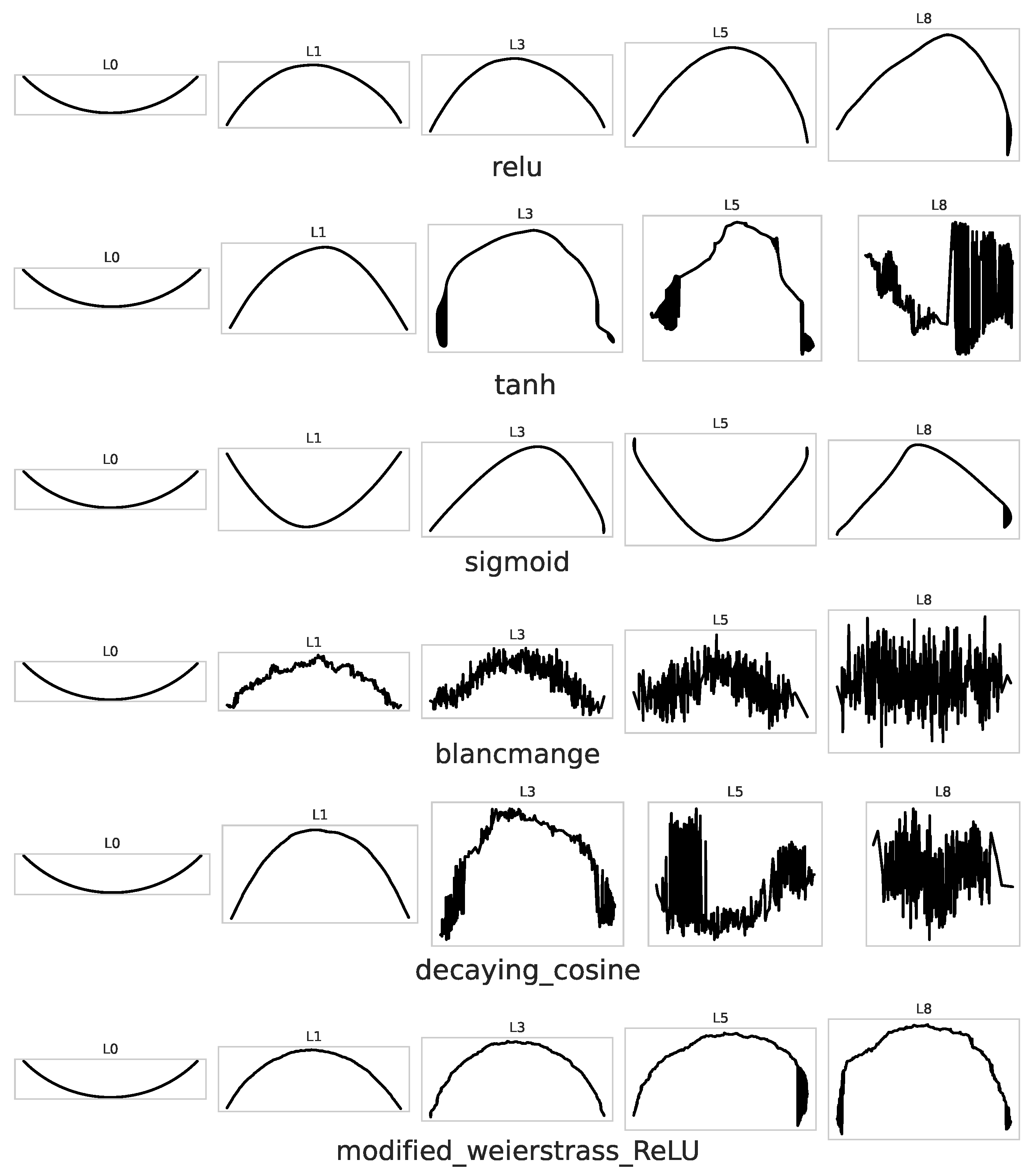
Figure 3.
PCA strips for activation functions.
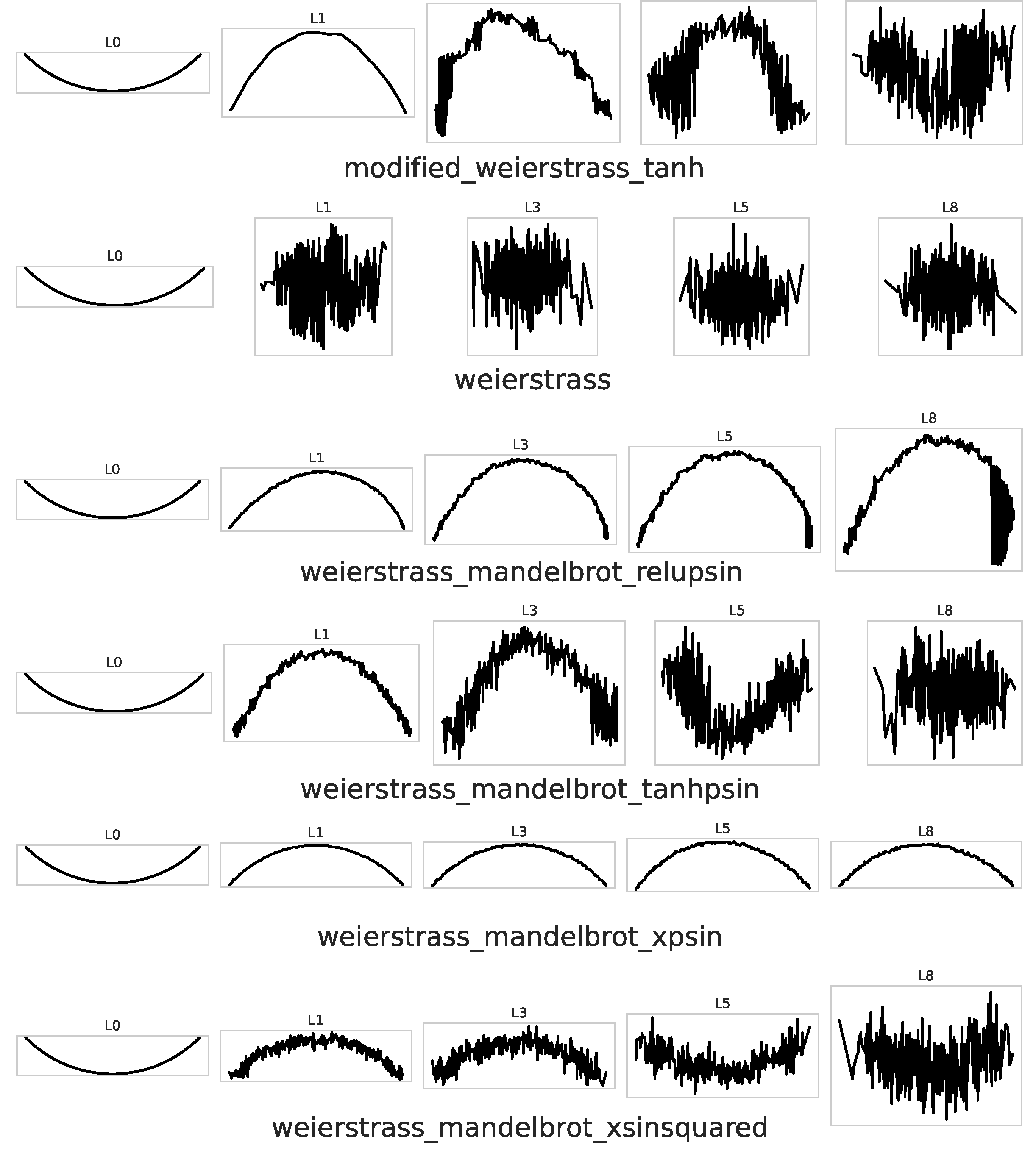

Table 1.
Results climate-model-simulation-crashes.
| Optimizer | Activation | Mean | Std | Max | Min |
|---|---|---|---|---|---|
| sgd | modified_weierstrass_tanh | 0.9148 | 0.0203 | 0.9506 | 0.8642 |
| sgd | sigmoid | 0.9140 | 0.0196 | 0.9444 | 0.8642 |
| sgd | tanh | 0.9140 | 0.0196 | 0.9444 | 0.8642 |
| adadelta | blancmange | 0.9140 | 0.0196 | 0.9444 | 0.8642 |
| sgd | relu | 0.9140 | 0.0196 | 0.9444 | 0.8642 |
| adam | blancmange | 0.9140 | 0.0196 | 0.9444 | 0.8642 |
| adadelta | sigmoid | 0.9140 | 0.0196 | 0.9444 | 0.8642 |
| sgd | blancmange | 0.9140 | 0.0196 | 0.9444 | 0.8642 |
| rmsprop | blancmange | 0.9140 | 0.0196 | 0.9444 | 0.8642 |
| adam | sigmoid | 0.9140 | 0.0196 | 0.9444 | 0.8642 |
Table 2.
Top-results diabetes dataset.
| Optimizer | Activation | Mean | Std | Max | Min |
|---|---|---|---|---|---|
| adam | modified_weierstrass_tanh | 0.7666 | 0.0231 | 0.8225 | 0.7013 |
| adadelta | modified_weierstrass_tanh | 0.7646 | 0.0207 | 0.8139 | 0.7273 |
| rmsprop | modified_weierstrass_tanh | 0.7644 | 0.0220 | 0.8225 | 0.7143 |
| adadelta | relu | 0.7609 | 0.0213 | 0.7965 | 0.7143 |
| adagrad | sigmoid | 0.7583 | 0.0210 | 0.8095 | 0.7143 |
| adagrad | tanh | 0.7554 | 0.0275 | 0.7965 | 0.6537 |
| adagrad | relu | 0.7506 | 0.0288 | 0.8009 | 0.6623 |
| adadelta | tanh | 0.7472 | 0.0222 | 0.7835 | 0.6970 |
| adam | tanh | 0.7420 | 0.0255 | 0.7922 | 0.6623 |
| adam | relu | 0.7409 | 0.0241 | 0.7922 | 0.6710 |
Table 3.
Top-results glass dataset.
| Optimizer | Activation | Mean | Std | Max | Min |
|---|---|---|---|---|---|
| adadelta | decaying_cosine | 0.5923 | 0.0700 | 0.7538 | 0.3846 |
| rmsprop | decaying_cosine | 0.5923 | 0.0689 | 0.7846 | 0.3846 |
| adam | decaying_cosine | 0.5869 | 0.0635 | 0.7077 | 0.3846 |
| adadelta | weierstrass_mandelbrot_xpsin | 0.5819 | 0.0624 | 0.7231 | 0.4615 |
| rmsprop | weierstrass_mandelbrot_xpsin | 0.5696 | 0.0703 | 0.7077 | 0.4000 |
| rmsprop | weierstrass_mandelbrot_xsinsquared | 0.5669 | 0.0500 | 0.6615 | 0.4615 |
| rmsprop | weierstrass_mandelbrot_tanhpsin | 0.5669 | 0.0675 | 0.7077 | 0.4154 |
| sgd | tanh | 0.5650 | 0.0680 | 0.7231 | 0.4615 |
| adadelta | blancmange | 0.5581 | 0.0713 | 0.7077 | 0.4000 |
| adam | tanh | 0.5558 | 0.0696 | 0.6923 | 0.4000 |
Table 4.
Top-results ionosphere dataset.
| Optimizer | Activation | Mean | Std | Max | Min |
|---|---|---|---|---|---|
| adam | modified_weierstrass_tanh | 0.9038 | 0.0271 | 0.9434 | 0.8396 |
| adam | relu | 0.8983 | 0.0354 | 0.9623 | 0.8302 |
| rmsprop | modified_weierstrass_tanh | 0.8965 | 0.0296 | 0.9340 | 0.8302 |
| adadelta | modified_weierstrass_tanh | 0.8936 | 0.0324 | 0.9434 | 0.8208 |
| rmsprop | relu | 0.8899 | 0.0395 | 0.9528 | 0.8113 |
| adadelta | relu | 0.8849 | 0.0494 | 0.9623 | 0.7547 |
| sgd | modified_weierstrass_tanh | 0.8686 | 0.0317 | 0.9151 | 0.8019 |
| adam | tanh | 0.8642 | 0.0346 | 0.9340 | 0.7925 |
| rmsprop | tanh | 0.8434 | 0.0415 | 0.9151 | 0.7736 |
| adam | decaying_cosine | 0.8413 | 0.0336 | 0.9057 | 0.7642 |
Table 5.
Top-results iris dataset.
| Optimizer | Activation | Mean | Std | Max | Min |
|---|---|---|---|---|---|
| adadelta | decaying_cosine | 0.9306 | 0.0376 | 0.9778 | 0.8444 |
| rmsprop | decaying_cosine | 0.9272 | 0.0372 | 0.9778 | 0.8222 |
| adam | decaying_cosine | 0.9256 | 0.0420 | 1.0000 | 0.8000 |
| sgd | relu | 0.9039 | 0.0675 | 1.0000 | 0.7333 |
| adagrad | relu | 0.8700 | 0.1242 | 1.0000 | 0.4889 |
| adam | relu | 0.8694 | 0.0737 | 1.0000 | 0.6667 |
| adadelta | relu | 0.8667 | 0.0790 | 1.0000 | 0.6444 |
| adadelta | weierstrass_mandelbrot_xpsin | 0.8656 | 0.0502 | 1.0000 | 0.7778 |
| rmsprop | weierstrass_mandelbrot_xpsin | 0.8606 | 0.0494 | 0.9556 | 0.7556 |
| rmsprop | relu | 0.8594 | 0.0738 | 0.9778 | 0.6667 |
Table 6.
Top-results seeds dataset.
| Optimizer | Activation | Mean | Std | Max | Min |
|---|---|---|---|---|---|
| adadelta | decaying_cosine | 0.8933 | 0.0406 | 0.9683 | 0.7937 |
| rmsprop | decaying_cosine | 0.8897 | 0.0405 | 0.9524 | 0.7937 |
| adam | decaying_cosine | 0.8893 | 0.0330 | 0.9524 | 0.8254 |
| rmsprop | weierstrass_mandelbrot_tanhpsin | 0.8885 | 0.0399 | 0.9683 | 0.8095 |
| adadelta | weierstrass_mandelbrot_xpsin | 0.8853 | 0.0424 | 0.9683 | 0.7937 |
| rmsprop | weierstrass_mandelbrot_xpsin | 0.8841 | 0.0378 | 0.9524 | 0.8095 |
| adadelta | weierstrass_mandelbrot_tanhpsin | 0.8750 | 0.0399 | 0.9524 | 0.7937 |
| rmsprop | weierstrass_mandelbrot_xsinsquared | 0.8730 | 0.0478 | 0.9365 | 0.7302 |
| sgd | tanh | 0.8730 | 0.0517 | 0.9524 | 0.7619 |
| rmsprop | weierstrass_mandelbrot_relupsin | 0.8687 | 0.0344 | 0.9365 | 0.7619 |
Table 7.
Top-results tic-tac-toe dataset.
| Optimizer | Activation | Mean | Std | Max | Min |
|---|---|---|---|---|---|
| adagrad | relu | 0.8083 | 0.0344 | 0.8646 | 0.7153 |
| adagrad | tanh | 0.7616 | 0.0508 | 0.8542 | 0.6319 |
| adagrad | modified_weierstrass_tanh | 0.7547 | 0.0899 | 0.8611 | 0.4444 |
| adadelta | modified_weierstrass_tanh | 0.7545 | 0.0256 | 0.8264 | 0.7153 |
| adam | modified_weierstrass_tanh | 0.7503 | 0.0253 | 0.8056 | 0.7083 |
| adam | relu | 0.7500 | 0.0277 | 0.8090 | 0.7083 |
| rmsprop | modified_weierstrass_tanh | 0.7498 | 0.0263 | 0.8125 | 0.6979 |
| adadelta | relu | 0.7443 | 0.0257 | 0.8160 | 0.7049 |
| rmsprop | relu | 0.7400 | 0.0257 | 0.8021 | 0.7049 |
| adagrad | sigmoid | 0.7237 | 0.0261 | 0.7917 | 0.6736 |
Table 8.
Top-results vehicle dataset.
| Optimizer | Activation | Mean | Std | Max | Min |
|---|---|---|---|---|---|
| adam | relu | 0.7973 | 0.0281 | 0.8543 | 0.7205 |
| rmsprop | relu | 0.7957 | 0.0304 | 0.8583 | 0.7244 |
| adadelta | relu | 0.7912 | 0.0293 | 0.8504 | 0.7362 |
| sgd | relu | 0.7857 | 0.0256 | 0.8425 | 0.7323 |
| adam | modified_weierstrass_tanh | 0.7685 | 0.0304 | 0.8268 | 0.6969 |
| rmsprop | modified_weierstrass_tanh | 0.7633 | 0.0330 | 0.8150 | 0.6614 |
| adadelta | modified_weierstrass_tanh | 0.7582 | 0.0286 | 0.8386 | 0.7008 |
| adam | tanh | 0.7541 | 0.0281 | 0.8110 | 0.6969 |
| adadelta | tanh | 0.7511 | 0.0309 | 0.8071 | 0.6890 |
| rmsprop | tanh | 0.7455 | 0.0374 | 0.8031 | 0.6575 |
Table 9.
Top-results vertebra-column dataset.
| Optimizer | Activation | Mean | Std | Max | Min |
|---|---|---|---|---|---|
| sgd | tanh | 0.8376 | 0.0310 | 0.9032 | 0.7742 |
| adadelta | tanh | 0.8215 | 0.0393 | 0.8817 | 0.7204 |
| adadelta | modified_weierstrass_tanh | 0.8185 | 0.0359 | 0.8817 | 0.7312 |
| adam | modified_weierstrass_tanh | 0.8172 | 0.0345 | 0.8710 | 0.7527 |
| rmsprop | modified_weierstrass_tanh | 0.8172 | 0.0348 | 0.8710 | 0.7527 |
| adam | tanh | 0.8156 | 0.0428 | 0.8925 | 0.7204 |
| rmsprop | tanh | 0.8142 | 0.0409 | 0.8925 | 0.7204 |
| rmsprop | relu | 0.8086 | 0.0406 | 0.8817 | 0.7204 |
| adadelta | relu | 0.8081 | 0.0416 | 0.8817 | 0.7097 |
| adam | relu | 0.8073 | 0.0438 | 0.8817 | 0.6882 |
Table 10.
Top-results wine dataset.
| Optimizer | Activation | Mean | Std | Max | Min |
|---|---|---|---|---|---|
| adam | blancmange | 0.9528 | 0.0275 | 1.0000 | 0.8889 |
| rmsprop | blancmange | 0.9500 | 0.0344 | 1.0000 | 0.8333 |
| adadelta | blancmange | 0.9472 | 0.0330 | 1.0000 | 0.8704 |
| adam | modified_weierstrass_tanh | 0.9463 | 0.0271 | 1.0000 | 0.8889 |
| adadelta | modified_weierstrass_tanh | 0.9431 | 0.0276 | 0.9815 | 0.8889 |
| rmsprop | modified_weierstrass_tanh | 0.9417 | 0.0378 | 1.0000 | 0.8148 |
| sgd | relu | 0.9384 | 0.0454 | 1.0000 | 0.8333 |
| adadelta | relu | 0.9352 | 0.0478 | 1.0000 | 0.8148 |
| adam | relu | 0.9343 | 0.0490 | 1.0000 | 0.7963 |
| sgd | modified_weierstrass_tanh | 0.9315 | 0.0408 | 1.0000 | 0.8333 |
Table 11.
Arc-length after the 4th and 8th hidden layer for twelve activation functions.
| Activation function |
arc-len |
arc-len |
Activation function |
arc-len |
arc-len |
|---|---|---|---|---|---|
| relu | weierstrass mandelbrot relupsin |
||||
| tanh | weierstrass mandelbrot tanhpsin |
||||
| sigmoid | blancmange | ||||
| weierstrass | decaying cosine |
||||
| weierstrass mandelbrot xpsin |
modified weierstrass tanh |
||||
| weierstrass mandelbrot xsinsquared |
modified weierstrass ReLU |
Disclaimer/Publisher’s Note: The statements, opinions and data contained in all publications are solely those of the individual author(s) and contributor(s) and not of MDPI and/or the editor(s). MDPI and/or the editor(s) disclaim responsibility for any injury to people or property resulting from any ideas, methods, instructions or products referred to in the content. |
© 2025 by the authors. Licensee MDPI, Basel, Switzerland. This article is an open access article distributed under the terms and conditions of the Creative Commons Attribution (CC BY) license (http://creativecommons.org/licenses/by/4.0/).
Copyright: This open access article is published under a Creative Commons CC BY 4.0 license, which permit the free download, distribution, and reuse, provided that the author and preprint are cited in any reuse.


