Submitted:
05 August 2025
Posted:
05 August 2025
You are already at the latest version
Abstract
Ship trajectory prediction plays an important role in numerous maritime applications and services. With the development of deep learning technology, the deep learning prediction method based on AIS (Automatic Identification System) data has become one of the hot topics in current maritime traffic research. However, the academic community currently generally focuses on connections between trajectory points while ignoring correlations among the dynamic information of trajectory points and the po-tential information of the dynamic information itself. Aiming at the problem of insuf-ficient modeling of the relationships among dynamic information in ship trajectory prediction, we propose MART (Multidimensional Attribute Relationship Transformer) model. This model introduces a simulated trajectory training strategy to obtain the Association Loss (AssLoss) for learning the associations among different dynamic in-formation; and uses the Distance Loss (DisLoss) to integrate the relative distance in-formation of the attribute embedding encoding to assist the model in understanding the relationships among different values in the dynamic information. We test the model on two AIS datasets, and the experiments show this model outperforms existing models (such as seq2seq, etc.) in long-term prediction tasks. This study reveals the im-portance of the relationship between attributes and the relative distance of attribute values in spatiotemporal sequence modeling.
Keywords:
AIS data
; deep learning
; ship trajectory prediction
; attribute association
; embedding encoding
1. Introduction
In the past few decades, maritime situation awareness and maritime surveillance have gradually become research hotspots, with the core objective of using multi-source data to achieve the maximum perception of maritime activities. Maritime safety is a very important field among them. Currently, there are various types of data related to maritime safety, and the most important of them is the AIS data provided by the Automatic Identification System (AIS)[1]. With the promotion and popularization of AIS equipment by the International Maritime Organization (IMO), the number of ships equipped with AIS equipment has been continuously increasing, accumulating a large amount of AIS data. This data contains key information such as longitude, latitude, speed over ground(SOG), course over ground(COG), Maritime Mobile Service Identity (MMSI), ship type, and motion state. The mining and utilization of its deep-level information provide data support for fields such as ship collision avoidance and anomaly detection. Among them, ship trajectory prediction is an important method for utilizing AIS data.
Ship trajectory prediction refers to using machine learning, deep learning or other related technologies to predict the future trajectory of ships based on historical ship trajectory data and environmental information[2]. Accurate ship trajectory prediction can be used for maritime traffic management[3], including tasks such as route planning[4,5,6], destination and arrival time prediction[7], maritime search and rescue operations[8,9], maritime abnormal traffic detection[10,11,12], etc., providing technical support for the intelligence of maritime supervision systems[13]. The mainstream ship trajectory prediction methods are mainly divided into two types. The first type relies on the ship motion model as prior knowledge and combines filtering methods or other clustering methods and then samples to obtain the final posterior prediction results. The simplest and most common motion model is the Nearly Constant Velocity (NCV) model[14], but it lacks consideration of complex situations. Then, scholars proposed the Kernel Density Estimation (KDE)[15] method for trajectory prediction. By marking the source trajectory and time in the historical data, it is possible to predict multiple possible paths of the trajectory. Based on the knowledge of historical trajectories, Mazzarella et al. [16] proposed the KB-PF (Particle Filter) method. They match the trajectory to be predicted with historical trajectories. If the matching fails, the NCV model is used, and if the matching is successful, the PF method is used for subsequent prediction. Rong et al. [17] proposed a Gaussian process model, which decomposes the ship motion into horizontal and vertical directions and calculates the position probabilities in these two directions, and updates the parameters of the Gaussian model through historical ship trajectories. However, the limitations of the above methods are quite obvious. Their predictions are based on the trajectory motion model, which can’t explain the existence of turning points, and the prediction time will become longer as the amount of data increases. At the same time, the filtering method is prone to the problem of error propagation and is not suitable for long-term prediction. The second type is the neural network-based method that has emerged in recent years. With the extensive application of neural network models in various fields and achieving state-of-the-art results, ship trajectory prediction has shifted from prediction using kinematic models to prediction using neural network and deep learning models. Given the sequential characteristics of ship trajectories, the structure of the Recurrent Neural Network (RNN) is very suitable for learning these features. To solve the long-term dependence problem in RNNs, its variant, the Long Short-Term Memory (LSTM) model, has emerged. Ma et al. [18] used RNN and LSTM models for multi-trajectory prediction, and the experimental results showed that the LSTM model performed better. Park et al. [19] understood the intentions of ships through trajectory prediction to prevent ship collisions. They used the Bi-LSTM model to learn the characteristics of ship trajectories from noisy trajectory points and achieved more accurate prediction results compared with the LSTM and GRU models in the final trajectory prediction. Due to the success of the seq2seq method in machine translation, some scholars have also applied it to trajectory prediction. Forti et al. [20] used LSTM as the encoder and decoder for long-term trajectory prediction and achieved better results compared with the Ornstein-Uhlenbeck stochastic process method. Capobianco et al. [21] selected Bi-LSTM as the encoder compared with the former and added the attention mechanism to solve the problem of long-distance dependence, improving the prediction accuracy of the model. The proposal of the Transformer model is another outstanding contribution in the field of deep learning. Its attention mechanism obtains the information of each token in the input sequence data simultaneously and makes prediction outputs in parallel, which enables the Transformer to learn the long-term dependence relationships existing in the data while speeding up the training speed of the model and successfully achieving state-of-the-art results in multiple fields. For example, Nguyen et al. [22] improved the Transformer to obtain the TrAISformer. They gridded the areas and connected various attribute information of the input after embedding as the input, and obtained the predicted trajectory through the method of probability sampling, which solved the multimodal and heterogeneous problems in ship trajectories to a certain extent. The multimodal problem of long-term prediction is shown in Figure 1. The blue trajectory is the real trajectory, while the yellow dotted line and the red dotted line are other possible trajectory directions. Since there are multiple reasonable possibilities for the future trajectory of the ship instead of a single definite trajectory, the modalities of different trajectories need to be modeled and predicted simultaneously.
In ship trajectory prediction, due to the difficulties encountered in data collection, most of the research in this direction mainly emphasizes dynamic ship information, such as position, speed and course. Most ship trajectory prediction methods also use these four types of dynamic information as the input of the model in experiments[23,24]. In order to solve the existing multimodal problems, many studies[18,19,20] attempt to merge trajectories with similar features into one category through methods such as clustering, so as to help the model achieve better prediction results in the form of labels and the like. However, this method is quite difficult for vast areas with complex trajectories, while Nguyen et al. [22] can solve the multimodal problem relatively well by using embedded vectors in the way of probability sampling. However, since only the dynamic information is separately embedded and then concatenated as the input, the model will actually only combine the information of the speed, course and position for understanding. It is unable to understand the relationships between attributes. As a result, when encountering unfamiliar trajectories, the model can’t start from the information of the trajectory itself, but matches it with the training data, leading to serious prediction errors. In addition, as a Transformer model originally used for NLP tasks, when texts and trajectories are transformed into another dimension through embedding, theoretically, the embedding encoding corresponding to the vocabulary of the text does not contain the relationships between words. However, when the position, SOG and COG attributes of the trajectory are transformed into embedding encodings, the relative distances in the embedding encoding actually represent the relative distances between the values of the corresponding attributes, which is something worthy of attention when applying embedding to trajectories.
In order to address the above challenges, we propose the MART (Multidimensional Attribute Relationship Transformer) model. Our main contribution lies in the improvement of the loss function. We propose two loss calculation methods, namely AssLoss (Association Loss) and DisLoss (Distance Loss), which respectively enhance the model's understanding of the relationships between different attributes and the relationships among different values within attributes.
2. Methodology
2.1. Problem Statement
In current ship trajectory prediction models, the mainstream approach is to improve model to better memorize the trajectory shape. However, this is often limited by the trajectory distribution in the training set. Moreover, due to the scarcity of trajectories in some areas, the model fails to fully understand those areas. We have selected the test trajectories shown in Figure 2 for demonstration. The test trajectories are drawn with blue lines in the figure and their names are indicated with red letters. Both trajectories are located in the marginal areas of the training range and have simple trajectory shapes.
We use different points of the test trajectory as starting points and let the model predict the subsequent trajectories. The trajectories before the starting points are input into the model. The prediction results are shown in Figure 3. The blue line in the figure represents the real trajectory. The green line represents the trajectory points at future moments calculated according to the SOG and COG of the real trajectory points. The red line represents the predicted trajectory of the TrAISformer.
As can be seen from the figure, the SOG and COG of this trajectory are highly consistent with the real situation of the trajectory. Therefore, the positions at future moments calculated according to the trajectory SOG and COG always coincide with the real positions of the trajectory. However, when the model makes predictions, the predicted points at the next moment of the input points always deviate greatly from the real positions. This indicates that the trained model fails to understand the relationship between the speed and course and the movement of the ship.
Moreover, in the embedding layer of the model, due to the insufficient distribution of training data in some areas, the embedding vectors corresponding to these areas are not well trained, and the model fails to understand the real-world meanings of the corresponding vector spaces. This is clearly shown in Figure 4. The y-values in the figure are the cosine similarities calculated from the latitude vectors that are adjacent in the real world within the latitude vector space. For the previous area where there is sufficient amount of data in the training scope, the vectors corresponding to adjacent latitudes have relatively high cosine similarities. However, for the latter area, because there is less trajectory data at some positions, the cosine similarities of some adjacent latitude embedding vectors are close to 0. This is also the reason why the model performs poorly in predicting areas with sparse trajectories, as the model doesn’t understand the actual meanings of the position vectors corresponding to these areas.
2.2. Model Structure
In order to achieve better prediction of ship trajectories, since the transformer can fully learn the long-term dependencies among sequential data and enable efficient parallel computing, we use it as the basic architecture of the model to construct a model based on the association of multi-dimensional attributes of trajectories. The structural diagram of the model is shown in Figure 5. The input data is composed of real trajectory data and simulated trajectory data. Each trajectory contains a certain number of trajectory points composed of four attributes: latitude, longitude, SOG and COG. Before the embedding layer, the input attribute values are cut at equal intervals to obtain the embedding encodings. The process of inputting data into the model is as follows: first, the input data passes through the embedding vectors. Secondly, the real trajectories and the simulated trajectories are concatenated, added with the position encodings, and then input into the multi-layer blocks composed of the attention layer and the feed-forward fully connected layer. After passing through the final linear layer, the unnormalized weights are obtained. The weights are re-divided into the parts of the real trajectories and the simulated trajectories. Then, both parts are combined with the weights of corresponding distribution, and the DisLoss and AssLoss are obtained through the CrossEntropyLoss (CE). Finally, the two calculated loss values are added to obtain the final loss value. The calculation formula of the final model loss is as follows:
The embedding layer maps attribute information to the vector space, and the four attributes of the trajectory point as input are mapped to the corresponding vector space through their respective embedding layers and connected to obtain the vector representation of the trajectory point.
After the real trajectory and simulated trajectory as inputs are mapped to the vector space through Embedding, they will be added to the position encoding. The function of position encoding is to add sequential position information to the sequence vector, because the attention mechanism of the transformer operates in parallel for each point vector. Without position encoding, changing the order between point vectors in the sequence vector will only affect the vector order in the output result and not the actual output value. But in reality, whether it's ship trajectories or long texts, once the order is disrupted, the information inside will be changed. So it is necessary to use positional encoding to inform the model of the positional relationships present in the sequence vectors.
The obtained vector containing positional information will be input into the Blocks layer, which includes masked multi head self attention and Feed Forward Network (FFN) layers. The role of the self attention module is to enable the model to simultaneously pay attention to all the vectors in the sequence vector, so as to learn the long-range dependencies that exist in the input sequence. For the input sequence vector x, the first step is to transform it into Q, K, V through three transformation matrices:
Then the obtained Q, K, V matrices will enter the attention layer, and the attention calculation formula is as follows:
In the formula, is the vector dimension, is the attention score. After calculating the matrix multiplication operation of and , it is necessary to divide by the square root of the vector dimension to scale the softmax result, making the calculation stable and preventing gradient explosion or vanishing. The softmax is to convert the result of the and matrices into weights that sum to 1. Then, the embedded vectors are cut in a multi-head manner, so that the model can distribute attention to other related positions in different sub-spaces, enhancing the expressive ability of the model. By using self attention layers to learn the relationships between trajectory points, and then using FFN to learn the relationships between position, SOG, and COG. Finally, after passing through the Blocks composed of multiple attention layers and fully connected layers, the probability of the predicted trajectory points is obtained through the final linear layer and softmax.
For the predicted probabilities of the output, we re-cut them into the probabilities of the predicted points of the simulated trajectories and the probabilities of the predicted points of the real trajectories. For the part of the simulated trajectories, we only calculate the loss values of the latitude and longitude to obtain the AssLoss. The reason for giving up the loss values of the speed and course is mainly that the simulated trajectories we generate are completely random without target information, and there is no learning value in the variation patterns of the speed and course of the purposeless trajectories. For the part of the real trajectories, we calculate the sum of the loss values of the four attributes to obtain the DisLoss. However, different from the former, the label weights are not one-hot vectors, but are obtained according to the distances between the embedding encodings and the real label encodings. We distribute the weights corresponding to the real labels according to the normal distribution, and provide the distance relationships between different values in the attributes to the model through this method.
2.3. Distance Loss
This trajectory prediction model and the mainstream text generation models both use the transformer structure, but the two input completely different types of data. When the vocabulary obtained after word segmentation of the text and the longitude and latitude input of the trajectory are projected through embedding, there is no relationship between the words in the former and the embedding encodings, while there is a relatively obvious correlation in the latter. The specific situation is shown in Figure 6.
Therefore, the characteristics of the embedding encodings of the attributes of the trajectory points can be applied to the loss function. The most commonly used loss function in the mainstream text generation models is the cross-entropy function, which is Equation (4), as follows:
In this formula, denotes the number of samples, denotes the number of categories, represents the true probability distribution, and represents the predicted probability distribution. In practical applications, the true category distribution often uses one-hot vectors. In text generation, one-hot vectors are used as the category distribution mainly because of the mutual exclusivity between words in the vocabulary. The probability distribution of the output vocabulary learned by the model does not always result in a unimodal probability distribution like a one-hot vector; instead, it may produce multiple possible alternative words. However, such a weight distribution can’t be predefined by us and must be learned by the model itself. In trajectory prediction, different output categories for each attribute are always mutually exclusive. Theoretically, all prediction results except the true result are incorrect. Figure 7 illustrates possible prediction scenarios. The black line represents the input trajectory, the green lines represent possible predicted results, and the yellow points represent the true trajectory points. Among the multiple predicted results in the figure, the best prediction is naturally the true result, followed by the closer purple position, and the worst is the farthest red position. In trajectory prediction, the closer the embedding encoding of the predicted result is to that of the true result, the smaller its loss should be. Therefore, in the cross-entropy function, embedding encodings closer to the true category should have a higher output probability. We can reflect this by modifying the true category distribution.
For the new true category probability distribution, we adopt a normal distribution to obtain the weights corresponding to each category. Figure 8 shows this probability distribution. In this figure, the weight corresponding to the true embedding encoding is 0.8, the weights corresponding to two adjacent embedding encodings are 0.1 each, and the weights of the remaining parts are still close to 0. The reason for this distribution is that the current grid cells are approximately 1km in both length and width. Including additional adjacent areas would result in excessive prediction errors. By modifying the true category distribution in this way, the model can consider nearby points of the true position as potential alternatives during the prediction process, thereby enhancing the model's generalization ability.
We refer to the improved loss function as Distance Loss (DisLoss), and its calculation formula is as follows:
In the formula, GD is the formula used to calculate the Gaussian distribution. and are the standard deviation and the mean value of the Gaussian distribution respectively. The former is a given value (in the paper, it is 0.5), and the latter is the embedding encoding corresponding to the true value. and are the true probability distribution and the predicted probability distribution respectively. "True" represents the true trajectory, and CE represents the cross-entropy loss function.
2.4. Association Loss
In the model prediction, the four attributes of latitude (lat), longitude (lon), sog and cog are selected as inputs mainly because the two position attributes represent the position information of the ship that we need to predict, and sog and cog represent the motion state of the ship. For the simplest NCV model, the position at the next moment can be predicted based on the current position, speed and time. By interpolating the original trajectory at equal time intervals, the time information has been added to the trajectory data as a kind of hidden information. Therefore, in fact, what we need is to enable the model to learn the relationships among these four attributes, so as to predict the position at the next moment and predict the corresponding motion state according to the possible target of the ship. However, when we apply the trained ship trajectory prediction model to the test, we find that the model does not always understand the relationship between the SOG, COG and position. The model only understands these four attributes as a complex feature and ignores the internal connections among the attributes.
Therefore, we add simulated random trajectory data to the training data to help the model understand the impact of heading and speed information on the ship's navigation, as shown in Figure 5. Both the simulated trajectory and the real trajectory go through the same model structure to obtain the final probability output. However, different from the real trajectory, for the simulated trajectory, there is no need to predict the sog and cog. Only the prediction loss of longitude and latitude needs to be calculated to enable the model to understand the relationships among the four attributes. The loss used to assist the model in understanding the correlations of the attributes is called AssLoss, and its calculation formula is as follows:
In the formula, and have the same meanings as those in the previous text, and Sim represents the simulated trajectory. And the method for generating the simulated trajectory is as follows:
| Algorithm 1 Generate_Simulated_Traj() |
| Description: Generate simulated trajectories . |
|
Input: the boundary of area , the maxmium of sog =30, the maxmium of cog =72, the length of trajectory . |
|
Output: . // Generate the origin position = random_point() // Generate the others point for i in 0: -1 do // Randomly generate the speed and direction = random_motion()0 = cal_point() ) end Return |
3. Experiment
In this section, we evaluated the MART model on two real AIS datasets and also added comparisons of experimental results with other models. In addition, we also conducted ablation experiments to evaluate the impact of each method on the experimental results. In order to facilitate the reproduction of the model proposed in the paper, we have made the code and dataset open-source https://github.com/sgxzz1/MART.
3.1. Datasets
The dataset information is shown in Table 1. The first dataset is the data of the Danish area open-sourced by https://github.com/CIA-Oceanix/TrAISformer. The other dataset is obtained by downloading from the official website of the Danish Maritime Authority and preprocessing. Both datasets contain AIS data of cargo ships and tankers. For the former dataset, the time range is from January 1, 2019, to March 31, 2019, and the regional range is from (, ) to (, ). The data from January 1 to March 10 is used as the training set, the data from March 11 to March 20 is used as the validation set, and the remaining data is used as the test set. In total, it contains 13,679 ship trajectory data.For the latter dataset, the time range is from September 1, 2023, to February 29, 2024, and the regional range is a rectangular area from (, ) to (, ). The data are randomly divided into a training set, a validation set, and a test set at a ratio of 8:1:1. In total, it contains 78,647 ship trajectory data. For the convenience of description, the former is called Area 1 and the latter is called Area 2. The data preprocessing method refers to[22]. The data of the two areas are shown in Figure 9.
3.2. Model Parameter
In the result display, all models with the transformer architecture use 8-layer Transformer blocks, and each layer uses 8-head attention. The unit grid size for longitude and latitude is , the unit of SOG is 1 knot, and the unit of COG is . The embedding lengths corresponding to each unit are 256, 256, 128, and 128 respectively. The length of the input historical trajectory is 3 hours, and the future trajectory for 15 hours is predicted. We train our model on a single NVIDIA A10 GPU. For the training of the model in Area 1, it takes about 1 hour, while for the model in Area 2, the training takes about 9 hours.
3.3. Evaluation Criteria
For the prediction error of each step t, due to the high calculation efficiency of the Haversine formula and the small error in short distance calculation, the Haversine distance between the real point and the predicted point is used to represent the prediction error:
In the formula, represents the radius of the Earth, and , , , represent the latitudes and longitudes of the predicted point and the actual point respectively. Due to the diversity of ship trajectories, we adopt the method of multiple sampling, generating multiple different trajectories through sampling and selecting the best one as the prediction result.
3.4. Comparative Experiment
We compared MART with different trajectory prediction models, including seq2seq [20], seq2seq_attn[21], and TrAISformer[22]. To ensure the input formats were as consistent as possible, we added embedding layers to all tested models. All models were evaluated in two areas, and the experimental results are presented in Figure 10. Table 2 shows the prediction errors of each model at the 5th, 10th, and 15th hours in both areas. The MART model outperformed all others in both areas, achieving a 9.5% improvement in accuracy for 15-hour predictions in Area 1 and 15.4% in Area 2. Across multiple time intervals and areas, the average error was reduced by approximately 10%-15%.
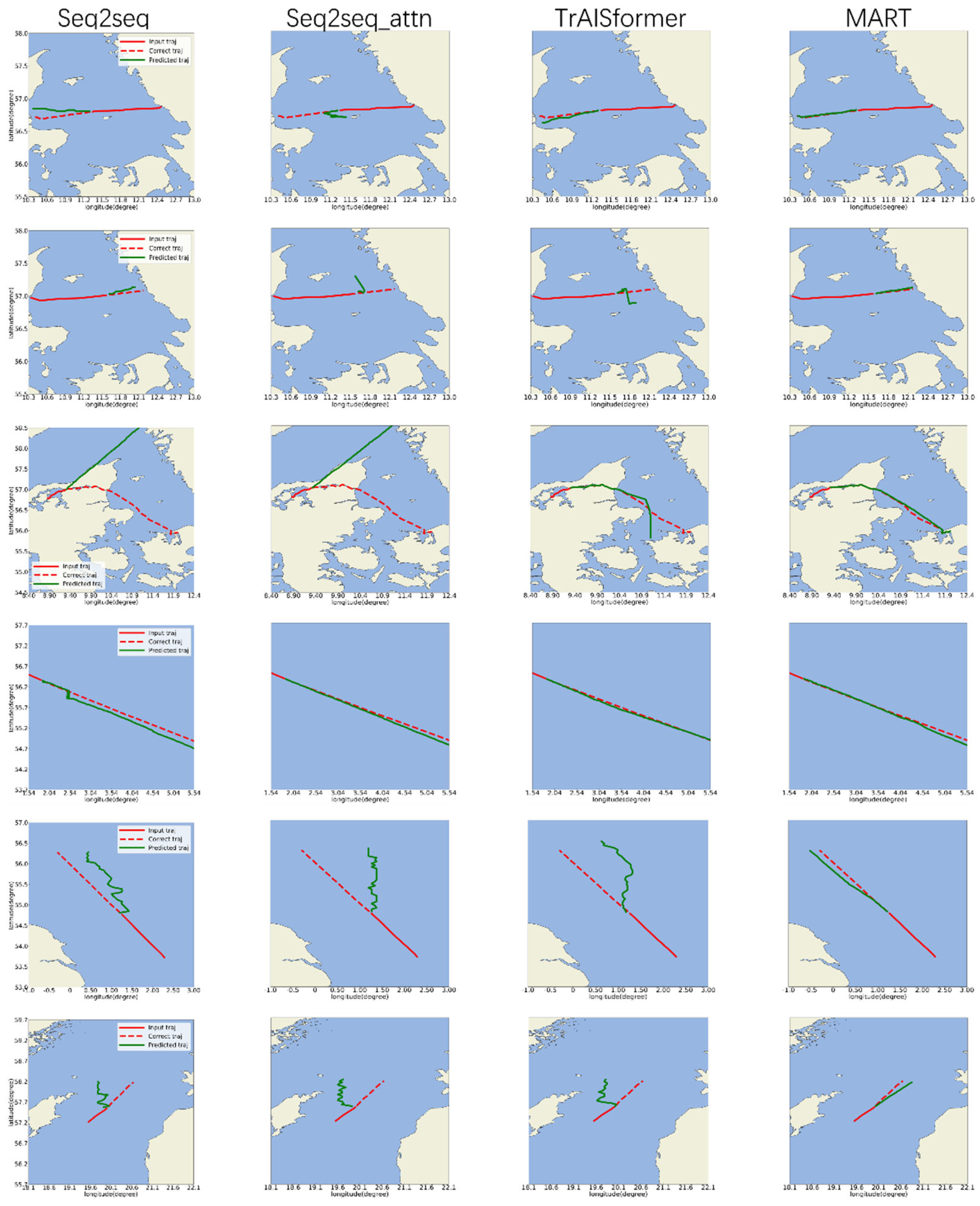
The improvement in accuracy is primarily attributed to the innovative methods we proposed. With DisLoss, we provided the model with prior knowledge of the relative distances between different values within the same attribute. Meanwhile, AssLoss enabled the model to learn the correlations between different attributes. As shown in Figure 12, the MART model accurately predicted simple straight-line routes. In contrast, the other three models exhibited significant deviations when predicting two straight-line trajectories in the test dataset. This discrepancy arises because they failed to capture the semantic meaning of direction, leading to immediate divergence from the true course starting from the first predicted point. Conversely, MART consistently predicted the initial point after the input trajectory accurately. Although it can’t guarantee perfectly accurate long-term predictions, it maintains the general directionality, ensuring that the predicted trajectories remain close to the ground truth. Moreover, MART demonstrated excellent memory retention for trajectories deviating from the main routes.
Moreover, since the positions corresponding to adjacent embedding encodings are closer in the actual space, we attempted to calculate whether the vectors corresponding to adjacent embedding encodings in the position vectors would be closer in the vector space. Thus, we calculated their cosine similarities, as shown in Figure 11. From the similarity graph of the longitude and latitude vector space in Area 1, it can be seen that the vectors corresponding to adjacent position embedding encodings always have a high similarity. In Area 2, except for the MART model, other models can’t learn the spatial vectors of these areas sufficiently due to the small number of trajectories in the marginal areas. As a result, the similarity of the adjacent embedding encoding vectors in these areas is low, which is also the reason why the other models perform poorly in predicting the test trajectories as shown in Figure 12. By adding simulated trajectories, we enable MART to fully learn and understand the position vectors of all areas in the space, so the similarity of adjacent vectors is always high.
Figure 11.
vector space cosine similarity graph: (a) Area 1 latitude vector cosine similarity; (b) Area 1 longitude vector cosine similarity; (c) Area 2 latitude vector cosine similarity; (d) Area 2 longitude vector cosine similarity
Figure 11.
vector space cosine similarity graph: (a) Area 1 latitude vector cosine similarity; (b) Area 1 longitude vector cosine similarity; (c) Area 2 latitude vector cosine similarity; (d) Area 2 longitude vector cosine similarity
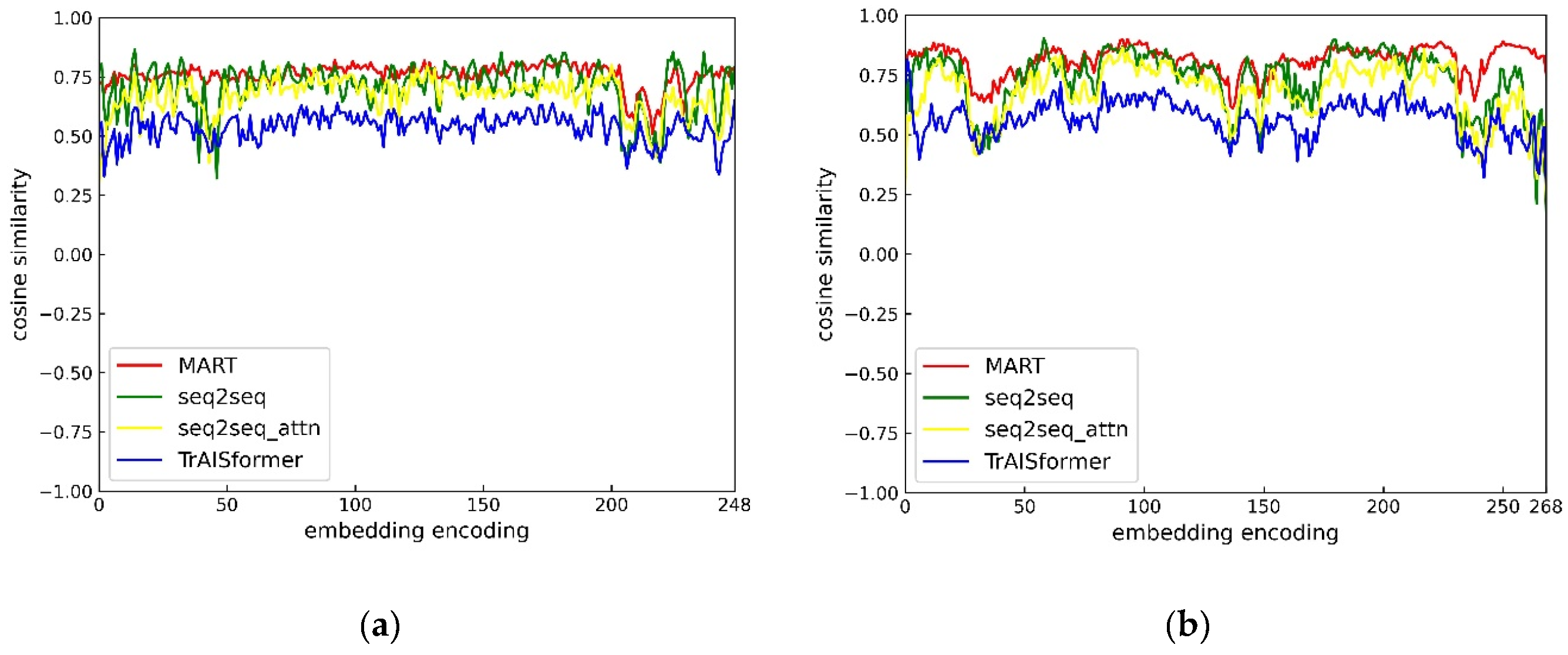
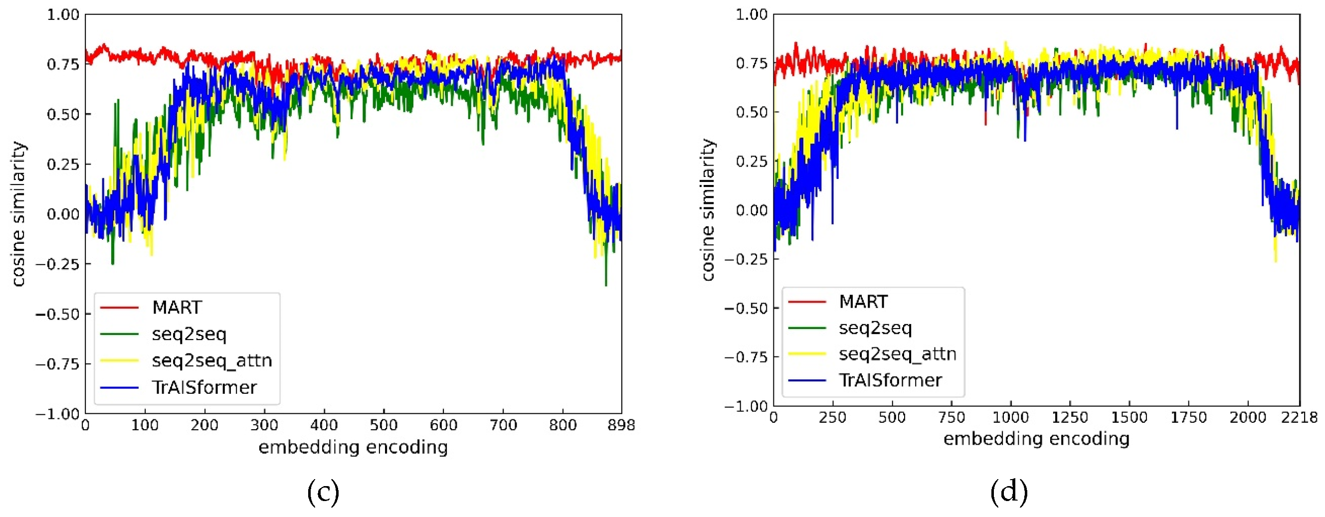
Figure 12.
Display of Multi Trajectory Prediction Results
3.5. Ablation Experiment
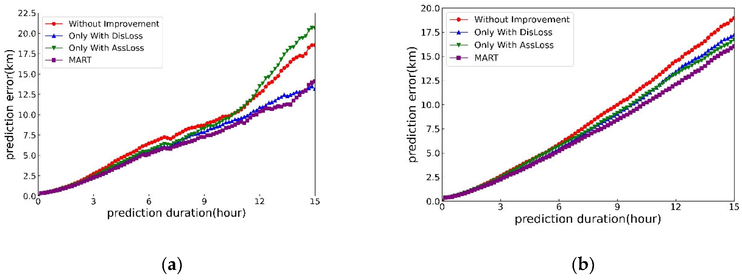
To demonstrate the improvement of each method on the prediction effect, we conducted ablation experiments and listed them in Table 3. As can be seen from the table, compared with the original model, the DisLoss method has improved the prediction effect in both regions. The AssLoss method has a better prediction effect within 10 hours in Region 1, but its prediction effect is worse than that of the original model after 10 hours. In Region 2, the effect after using this method is generally better than that of the original model. And MART, composed of the two improvement methods, has the best prediction effect in most cases in both regions. This also demonstrates the effectiveness of these two improvement methods, effectively proving that providing the relationship between attributes and the distance between attribute values to the model can indeed help the model achieve better results.
Figure 13.
Multi model prediction results: (a) Prediction results for Area 1; (b) Prediction results for Area 2
Figure 13.
Multi model prediction results: (a) Prediction results for Area 1; (b) Prediction results for Area 2
4. Conclusion
In this study, we established associations between the four attributes of the trajectory input and the embedding encodings, and provided this information to the model by improving the calculation of the loss function. Meanwhile, we incorporated simulated trajectories into the training to enable the model to understand the associations between the input attributes. Through the improvement of the above methods, we achieved enhancements to the original model and obtained optimal prediction results. By comparing the results of the ablation experiment, we verified the significance of each component of the method in improving the model.
5. Discussion
Since the two improvement methods proposed above do not actually involve modifications to the structure of the transformer model, theoretically, they are both transferable methods, and it is feasible to attempt to transplant them into other models, such as recurrent neural networks. However, as the above methods are all based on probability sampling experiments, when transplanting them, it is necessary to perform grid processing on the data, converting continuous values into discrete values to facilitate the final sampling generation.
Although we have attempted to enable the model to have a deeper understanding of the essence of the route data attributes, in essence, it still relies on the model's memory of the trajectory routes. The probability distribution of the predictions is essentially the distribution of the routes that appear in the training set. Therefore, it is difficult for the model to predict routes that do not exist in the training set. Our idea of making the model learn the relationship between position and speed is also based on this consideration. However, even if the model correctly predicts the position at the next moment based on the existing position and speed, the lack of speed information may still lead to prediction failures. This is also a drawback of the model trained based on existing trajectories. If it is to be used for more complex trajectory prediction, we need to add other information to the model for training, including but not limited to the destination of the ship, the behavioral objectives, and possible weather factors. However, since the destination and behavioral objectives should remain unchanged during a normal voyage, they can’t be directly connected as inputs like dynamic information such as position and speed, and a more reasonable way of adding them is required. For ship trajectories affected by weather factors, it is necessary to collect weather information that may affect the ship's navigation and associate it with the ship's trajectories in the corresponding areas and at specific moments, which will be a very challenging and research-worthy direction.
Author Contributions
Conceptualization, Methodology, Investigation and Writing - Original draft, Senyang Zhao; Data curation and Writing - review & editing, Wei Guo and Yi Liu. All authors have read and agreed to the published version of manuscript.
Funding
This research received no external funding.
Data Availability Statement
Data available within the article.
Conflicts of Interest
The authors declare no conflicts of interest.
References
- Chen, C.-H.; Khoo, L.P.; Chong, Y.T.; Yin, X.F. Knowledge Discovery Using Genetic Algorithm for Maritime Situational Awareness. Expert Systems with Applications 2014, 41, 2742–2753. [Google Scholar] [CrossRef]
- Tu, E.; Zhang, G.; Mao, S.; Rachmawati, L.; Huang, G.-B. Modeling Historical AIS Data For Vessel Path Prediction: A Comprehensive Treatment 2022.
- Liu, C.; Li, Y.; Jiang, R.; Du, Y.; Lu, Q.; Guo, Z. TPR-DTVN: A Routing Algorithm in Delay Tolerant Vessel Network Based on Long-Term Trajectory Prediction. Wireless Communications and Mobile Computing 2021, 2021, 6630265. [Google Scholar] [CrossRef]
- Nguyen, X.-P.; Dang, X.-K.; Do, V.-D.; Corchado, J.M.; Truong, H.-N. Robust Adaptive Fuzzy-Free Fault-Tolerant Path Planning Control for a Semi-Submersible Platform Dynamic Positioning System With Actuator Constraints. IEEE Trans. Intell. Transport. Syst. 2023, 24, 12701–12715. [Google Scholar] [CrossRef]
- Bi, J.; Cheng, H.; Zhang, W.; Bao, K.; Wang, P. Artificial Intelligence in Ship Trajectory Prediction. JMSE 2024, 12, 769. [Google Scholar] [CrossRef]
- Dang, X.K.; Truong, H.N.; Do, V.D. A Path Planning Control for a Vessel Dynamic Positioning System Based on Robust Adaptive Fuzzy Strategy. Automatika 2022, 63, 580–592. [Google Scholar] [CrossRef]
- Guan, M.; Cao, Y.; Cheng, X. Research of AIS Data-Driven Ship Arrival Time at Anchorage Prediction. IEEE Sensors J. 2024, 24, 12740–12746. [Google Scholar] [CrossRef]
- Ou, Z.; Zhu, J. AIS Database Powered by GIS Technology for Maritime Safety and Security. J. Navigation 2008, 61, 655–665. [Google Scholar] [CrossRef]
- Varlamis, I.; Tserpes, K.; Sardianos, C. Detecting Search and Rescue Missions from AIS Data. In Proceedings of the 2018 IEEE 34th International Conference on Data Engineering Workshops (ICDEW); IEEE: Paris, April, 2018; pp. 60–65. [Google Scholar]
- Venskus, J.; Treigys, P.; Markevičiūtė, J. Unsupervised Marine Vessel Trajectory Prediction Using LSTM Network and Wild Bootstrapping Techniques. NAMC 2021, 26, 718–737. [Google Scholar] [CrossRef]
- Olesen, K.V.; Boubekki, A.; Kampffmeyer, M.C.; Jenssen, R.; Christensen, A.N.; Hørlück, S.; Clemmensen, L.H. A Contextually Supported Abnormality Detector for Maritime Trajectories. JMSE 2023, 11, 2085. [Google Scholar] [CrossRef]
- Jurkus, R.; Venskus, J.; Markevičiūtė, J.; Treigys, P. Enhancing Maritime Safety: Estimating Collision Probabilities with Trajectory Prediction Boundaries Using Deep Learning Models. Sensors 2025, 25, 1365. [Google Scholar] [CrossRef]
- Zhang, X.; Fu, X.; Xiao, Z.; Xu, H.; Qin, Z. Vessel Trajectory Prediction in Maritime Transportation: Current Approaches and Beyond. IEEE Transactions on Intelligent Transportation Systems 2022, 23, 19980–19998. [Google Scholar] [CrossRef]
- Rong Li, X.; Jilkov, V.P. Survey of Maneuvering Target Tracking. Part I. Dynamic Models. IEEE Transactions on Aerospace and Electronic Systems 2003, 39, 1333–1364. [Google Scholar] [CrossRef]
- Ristic’, B.; Scala’, B.L.; Morelande’, M.; Gordon, N. Statistical Analysis of Motion Patterns in AIS Data: Anomaly Detection and Motion Prediction.
- Mazzarella, F.; Arguedas, V.F.; Vespe, M. Knowledge-Based Vessel Position Prediction Using Historical AIS Data. In Proceedings of the 2015 Sensor Data Fusion: Trends, Solutions, Applications (SDF); IEEE: Bonn, Germany, October, 2015; pp. 1–6. [Google Scholar]
- Rong, H.; Teixeira, A.P.; Guedes Soares, C. Ship Trajectory Uncertainty Prediction Based on a Gaussian Process Model. Ocean Engineering 2019, 182, 499–511. [Google Scholar] [CrossRef]
- Ma, H.; Zuo, Y.; Li, T. Vessel Navigation Behavior Analysis and Multiple-Trajectory Prediction Model Based on AIS Data. Journal of Advanced Transportation 2022, 2022, 6622862. [Google Scholar] [CrossRef]
- Park, J.; Jeong, J.; Park, Y. Ship Trajectory Prediction Based on Bi-LSTM Using Spectral-Clustered AIS Data. JMSE 2021, 9, 1037. [Google Scholar] [CrossRef]
- Forti, N.; Millefiori, L.M.; Braca, P.; Willett, P. Prediction Oof Vessel Trajectories From AIS Data Via Sequence-To-Sequence Recurrent Neural Networks. In Proceedings of the ICASSP 2020 - 2020 IEEE International Conference on Acoustics, Speech and Signal Processing (ICASSP); May 2020; pp. 8936–8940. [Google Scholar]
- Capobianco, S.; Millefiori, L.M.; Forti, N.; Braca, P.; Willett, P. Deep Learning Methods for Vessel Trajectory Prediction Based on Recurrent Neural Networks. IEEE Transactions on Aerospace and Electronic Systems 2021, 57, 4329–4346. [Google Scholar] [CrossRef]
- Nguyen, D.; Fablet, R. A Transformer Network With Sparse Augmented Data Representation and Cross Entropy Loss for AIS-Based Vessel Trajectory Prediction. IEEE Access 2024, 12, 21596–21609. [Google Scholar] [CrossRef]
- Li, H.; Lam, J.S.L.; Yang, Z.; Liu, J.; Liu, R.W.; Liang, M.; Li, Y. Unsupervised Hierarchical Methodology of Maritime Traffic Pattern Extraction for Knowledge Discovery. Transportation Research Part C: Emerging Technologies 2022, 143, 103856. [Google Scholar] [CrossRef]
- Li, H.; Jiao, H.; Yang, Z. Ship Trajectory Prediction Based on Machine Learning and Deep Learning: A Systematic Review and Methods Analysis. Engineering Applications of Artificial Intelligence 2023, 126, 107062. [Google Scholar] [CrossRef]
Figure 1.
Multimodal Problem Presentation.
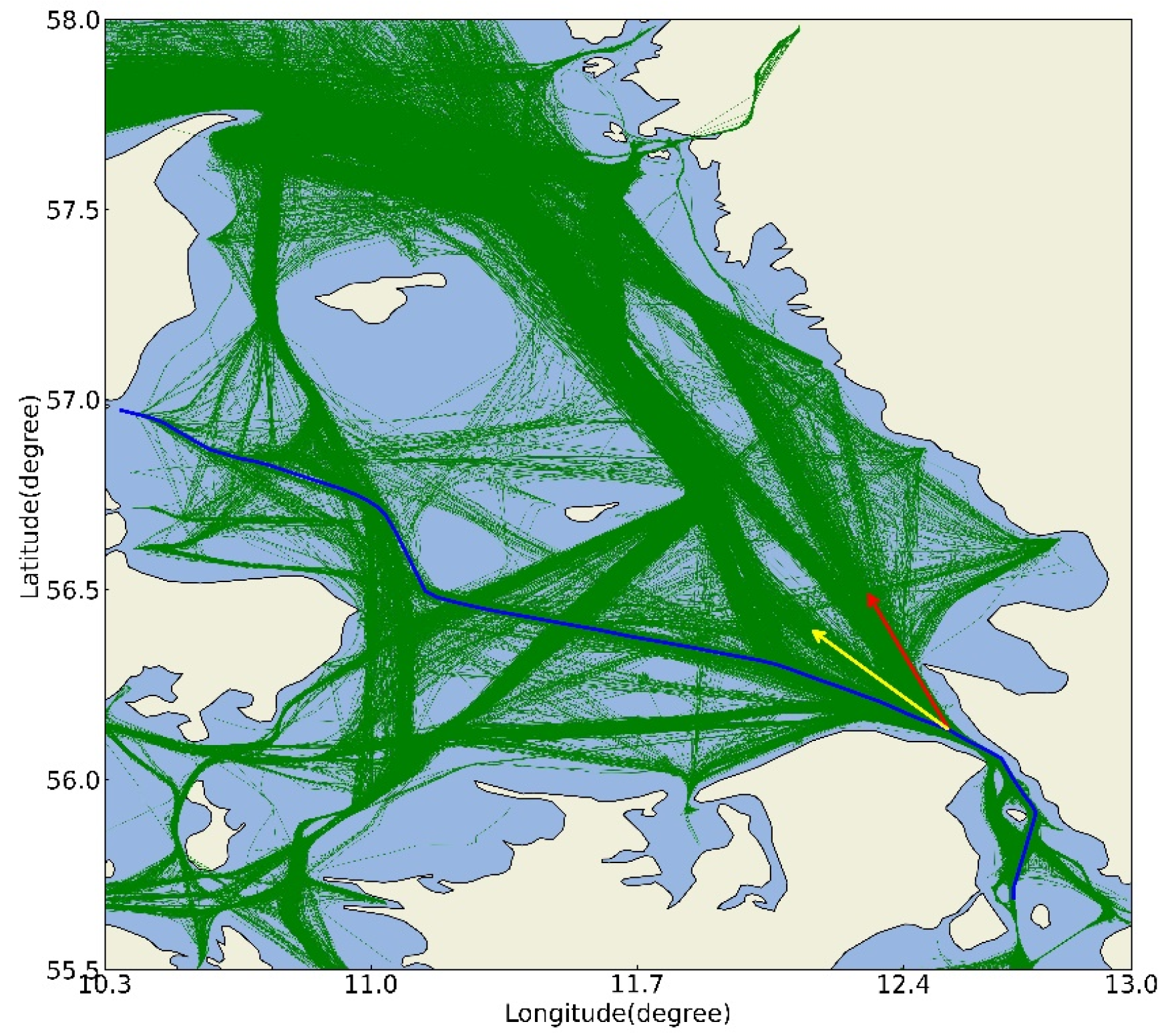
Figure 2.
Test Trajectory Display.
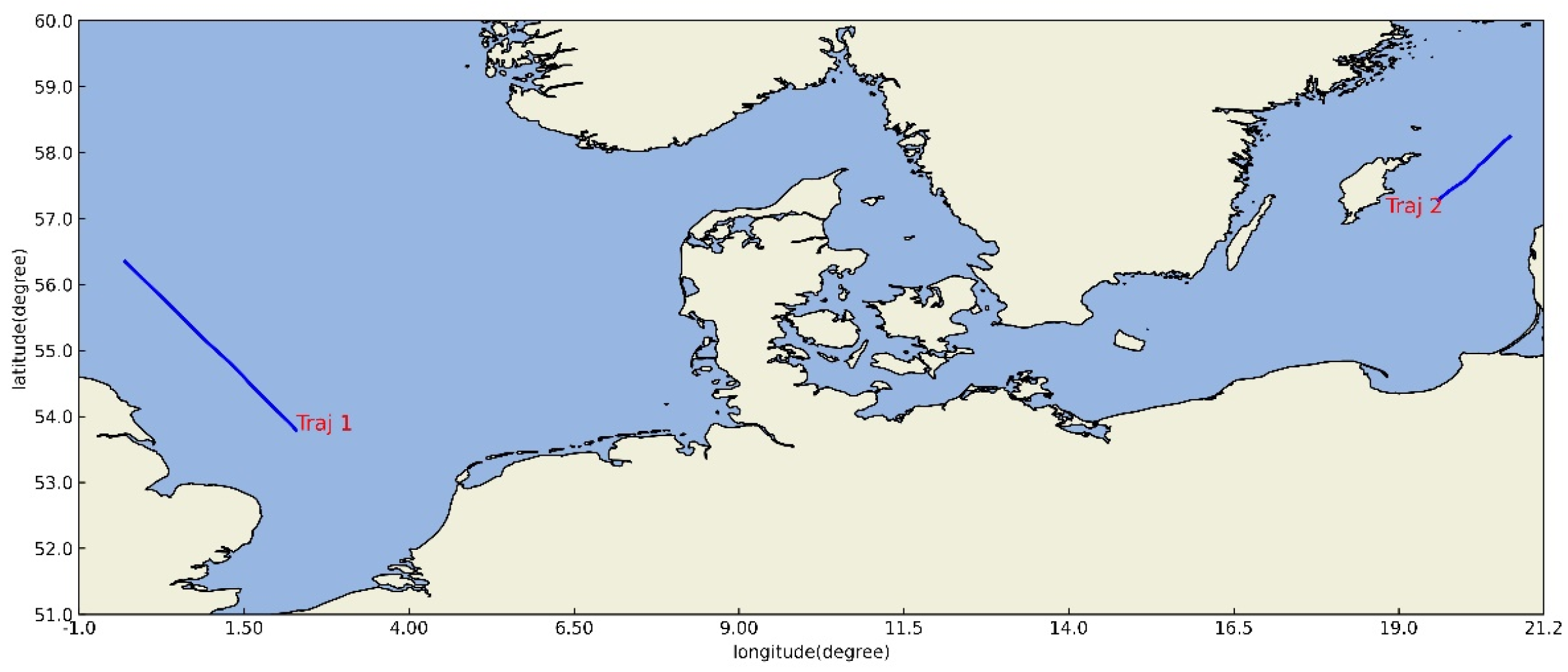
Figure 3.
test result: (a) Trajectory 1 prediction results; (b) Trajectory 2 prediction results.
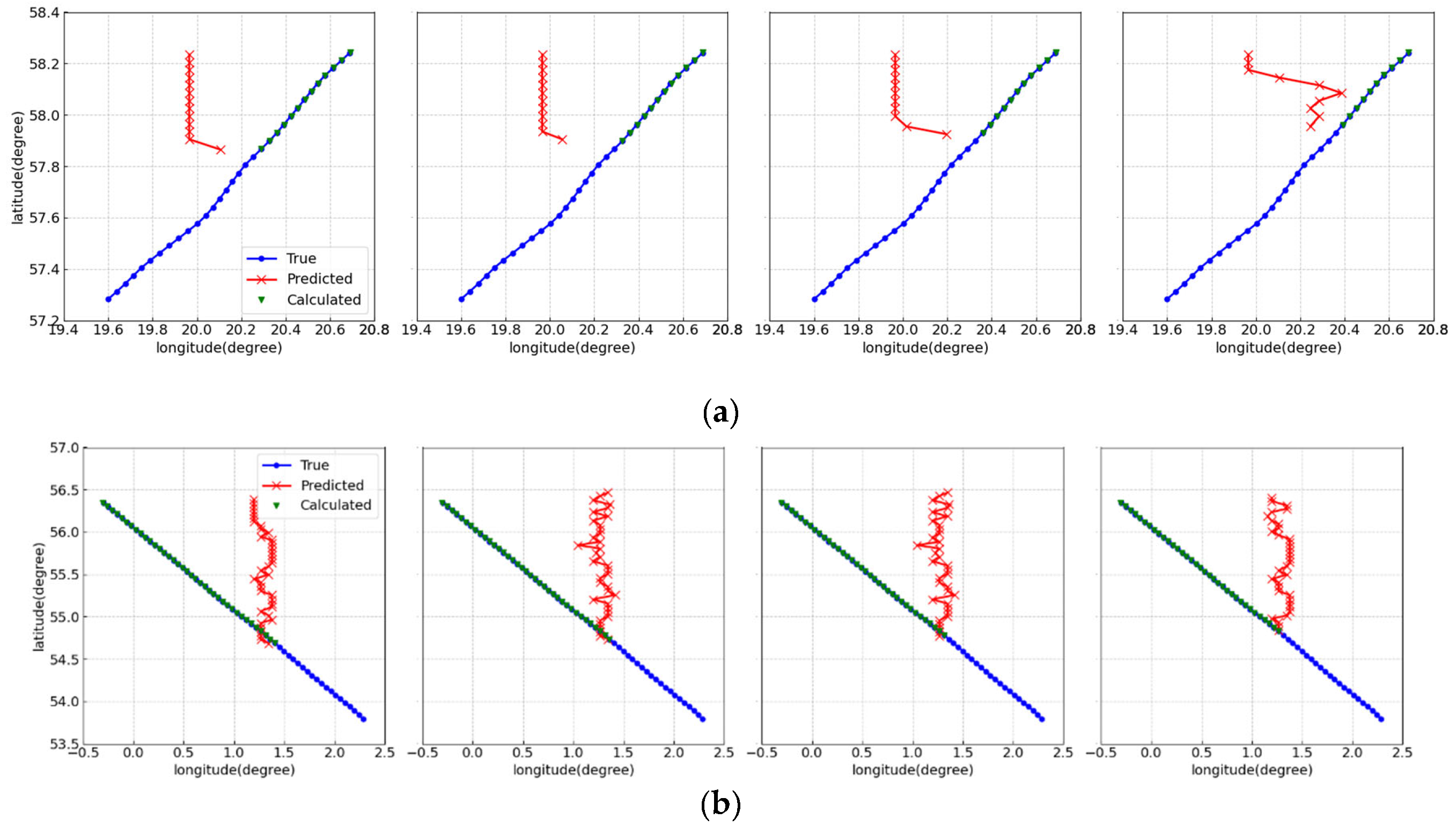
Figure 4.
TrAISformer Vector Space Similarity Graph: (a) Area 1 Latitude Vector Cosine Similarity; (b) Area 2 Latitude Vector Cosine Similarity.
Figure 4.
TrAISformer Vector Space Similarity Graph: (a) Area 1 Latitude Vector Cosine Similarity; (b) Area 2 Latitude Vector Cosine Similarity.
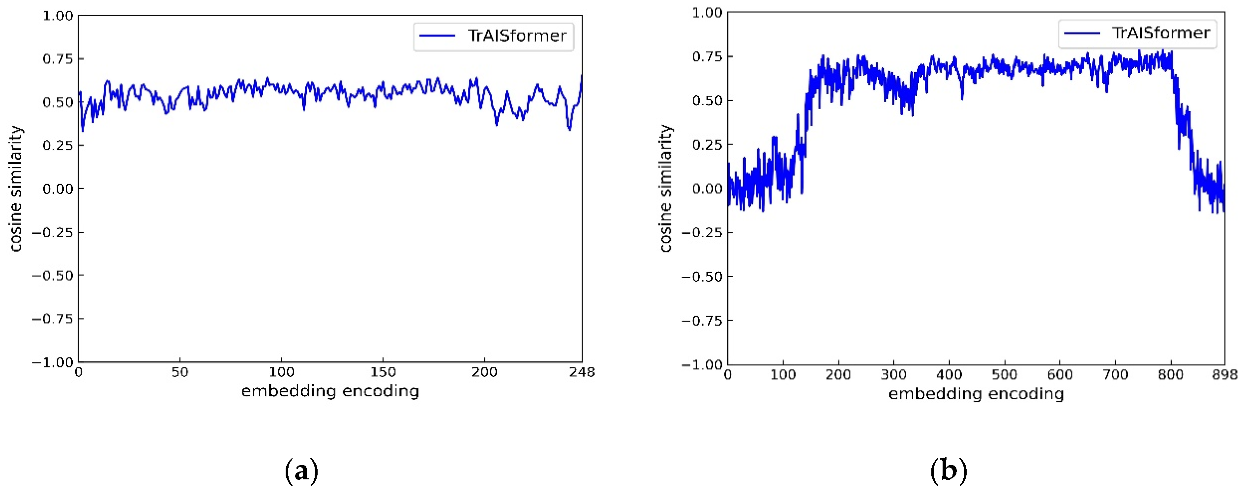
Figure 5.
Architecture of Ship Trajectory Prediction Model.
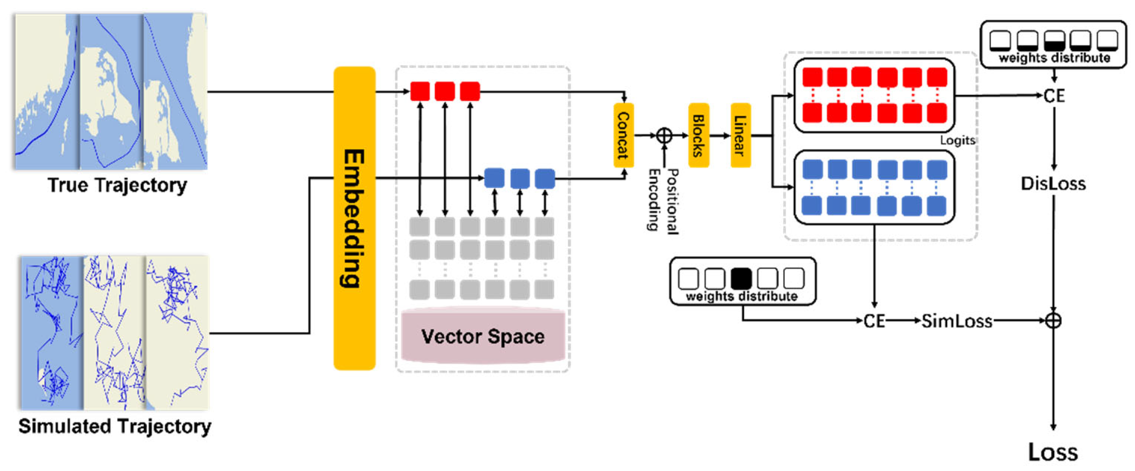
Figure 6.
Text and Trajectory Corresponding Embedding Encoding Example.
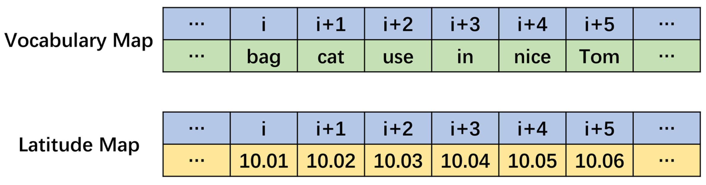
Figure 7.
Schematic Diagram of Trajectory Prediction.
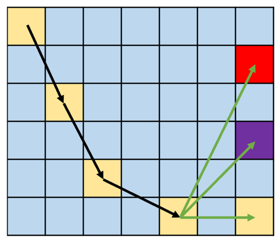
Figure 8.
Real Category Probability Distribution(, ).
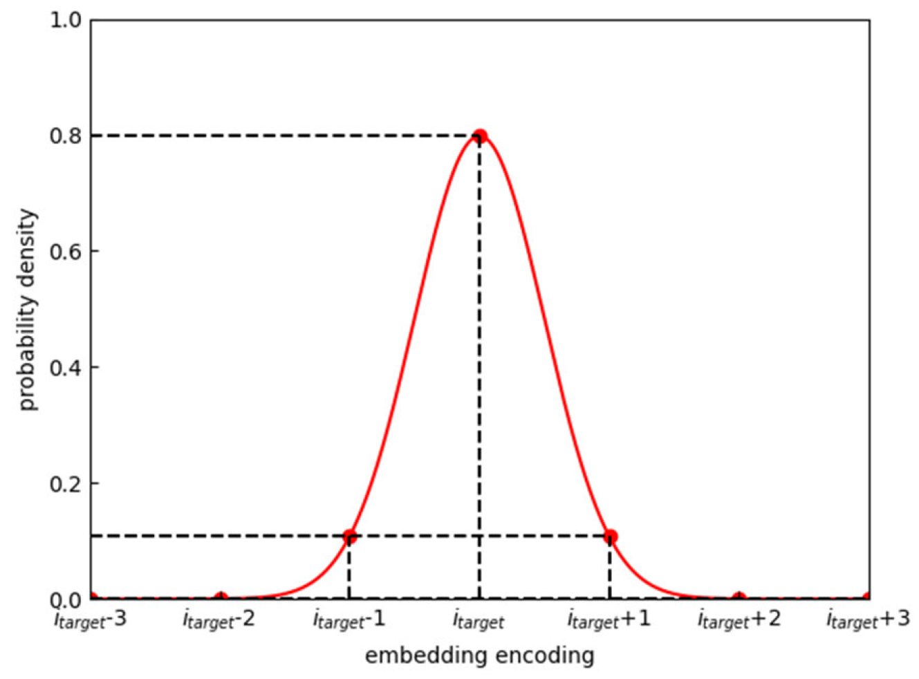
Figure 9.
Preprocessed dataset display: (a) Area 1; (b) Area 2.
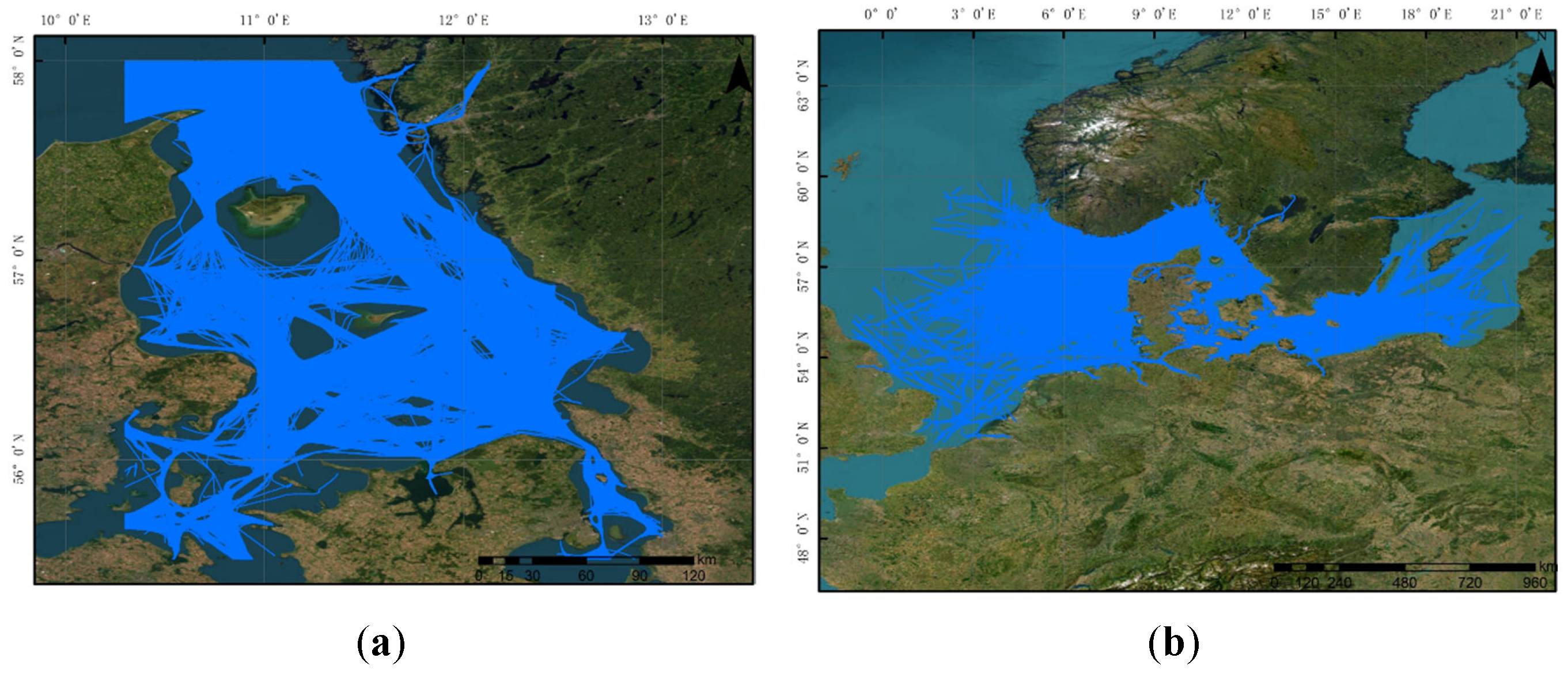
Figure 10.
Multi model prediction results: (a) Prediction results for Area 1; (b) Prediction results for Area 2.
Figure 10.
Multi model prediction results: (a) Prediction results for Area 1; (b) Prediction results for Area 2.
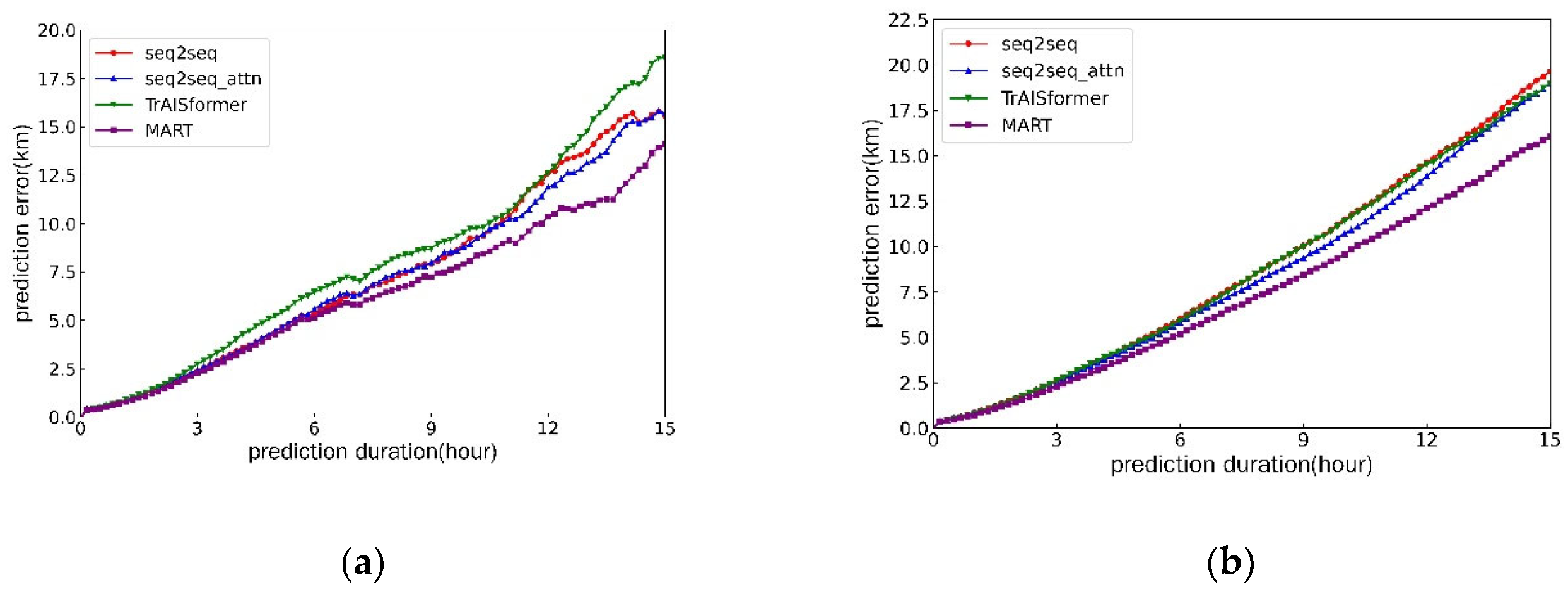

Table 1.
Datasets Display.
| Datasets | Time range | Spatial range | Data volume |
| Area 1 | 2019.1.1-2019.3.31 | (55.5°, 10.3°)-(58°, 13°) | 13679 |
| Area 2 | 2023.9.1-2024.2.29 | (51°, -1°)-(60°, 21.2°) | 78647 |
Table 2.
Multi Model Prediction Error Table (unit: km)
| Model | 5h(Area 1) | 10h(Area 1) | 15h(Area 1) | 5h(Area 2) | 10h(Area 2) | 15h(Area 2) |
| seq2seq | 4.43 | 9.24 | 15.58 | 4.83 | 11.49 | 19.64 |
| seq2seq_attn | 4.46 | 8.93 | 15.68 | 4.64 | 10.72 | 18.99 |
| TrAISformer | 5.22 | 9.76 | 18.56 | 4.74 | 11.40 | 18.97 |
| MART | 4.30 | 8.07 | 14.10 | 4.19 | 9.57 | 16.04 |
Table 3.
Table of Ablation Experiment (unit: km)
| Model | 5h(Area 1) | 10h(Area 1) | 15h(Area 1) | 5h(Area 2) | 10h(Area 2) | 15h(Area 2) |
| Without Improvement | 5.22 | 9.76 | 18.56 | 4.74 | 11.40 | 18.97 |
| Without DisLoss | 4.62 | 8.81 | 13.14 | 4.35 | 10.33 | 17.20 |
| Without AssLoss | 4.64 | 9.26 | 20.64 | 4.67 | 10.40 | 16.74 |
| MART | 4.30 | 8.07 | 14.10 | 4.19 | 9.57 | 16.04 |
Disclaimer/Publisher’s Note: The statements, opinions and data contained in all publications are solely those of the individual author(s) and contributor(s) and not of MDPI and/or the editor(s). MDPI and/or the editor(s) disclaim responsibility for any injury to people or property resulting from any ideas, methods, instructions or products referred to in the content. |
© 2025 by the authors. Licensee MDPI, Basel, Switzerland. This article is an open access article distributed under the terms and conditions of the Creative Commons Attribution (CC BY) license (http://creativecommons.org/licenses/by/4.0/).
Copyright: This open access article is published under a Creative Commons CC BY 4.0 license, which permit the free download, distribution, and reuse, provided that the author and preprint are cited in any reuse.


