
Submitted:
31 July 2025
Posted:
01 August 2025
You are already at the latest version
Abstract
This paper presents an investigation of the rotational lift production of translating and rotating wings within a small insect’s Reynolds numbers range. Using the Reynolds number 1200 of a bumble bee, three wing section profiles are studied; a circular cylinder model as the reference of a blunt body for which the well known Magnus effect will occur, a flat plate model as the reference of a sharp body for which the Kramer effect will occur and finally, an elliptical cylinder model, as a transition case. Direct force measurement and the particle image velocimetry (PIV) experiment have been performed in order to measure the lift produced and to bring out the surrounding flow velocity. The Kutta-Joukowski theorem has been applied on the PIV results. The experimental results are analyzed and verified with the comparison of computational results. In general, there is a reasonable agreement between the experimental and computational results. The results confirm that Magnus effect has been effectively observed for the circular cylinder model and no Kramer effect is observed for the flat plate model. Finally, the elliptical cylinder model appears not to be blunt enough for the Magnus effect to occur and not to be sharp enough for the Kramer effect to occur.
Keywords:
Kramer effect
; Magnus effect
; rotational lift
1. Introduction
The Unmanned Air Vehicles (UAV’s) or Bio-mimetic Air Vehicle s (BAV’s) are being used as a low-cost and efficient solution in various fields for security, surveillance applications or remote control. Therefore, the research towards the aerodynamics of insect flapping flight becomes an important role in recent years. Indeed it has been proven [1] that insect’s wings ranging from 1 to 100 mm in wingspan typically produce 2 or 3 times more lift than can be accounted for by conventional aerodynamics. Moreover, flapping wings improve, at small scales, both maneuverability and energy efficiency which is a great asset, for example, in order to hover.
The difference between actual planes and insect’s flight mainly rely on the Reynolds number. For higher Reynolds numbers case of actual planes, potential theory provides fairly accurate analysis. However, as the Reynolds number gets smaller, the viscous effect becomes important and is no longer negligible. That is why, for insects or small birds for which the Reynolds number is between 101 and 104, the aerodynamic principles are fundamentally different. Between this range of Reynolds number, several studies have been conducted in order investigate the impact of this parameters on the force produced. For example, Daniel K Hope, Anthony M DeLuca and Ryan P O’Hara investigated the behavior of a Manduca sexta inspired biomimetic wing as a function of Reynolds number by measuring the aerodynamic forces produced by varying the characteristic wing length and testing at air densities from atmospheric to near vacuum [2]. Therefore, the study of the unsteady nature of insect flight and so the complex flow surrounding their flapping wings seems to be a promising way to improve our knowledge and then to innovate our real-world applications.
When the insects and small birds hover with their small wings, the Reynolds number would have been too small to support their weight in a quasi-steady-state point of view. However, as you may notice, they can. The reason for this would be the quasi-steady translational lift and some phenomena of unsteady lift-enhancement mechanisms. Four of them will be briefly explained [3]. The first one is Delayed stall of leading edge vortex (LEV) [4,5]. When the wing accelerates, a starting vortex is created in order to keep the Kutta–Joukowski condition satisfied. As a response, a bound vortex will appear and this one will increase the circulation around the wing and then the lift production [5]. While the wing accelerates, this vortex can be maintained for a few chord lengths. It becomes totally unsteady.
The second one is the interaction between the wing and the wake, called wake capture. When a wing meets the wake created during the previous stroke after reversing its direction, the effective flow speed surrounding the airfoil increases which generates a second force peak. As it is claimed [6], even if the wing suddenly stops after just the rotation, a consequent amount of lift production is still noticed thanks to the previous wake. The third one is and added-mass acceleration. The added mass is the inertia added to a system because an accelerating or decelerating body must move some volume of surrounding fluid as it moves through it. Added mass is an intuitive issue because the body and the fluid cannot occupy the same physical space in the same time. For simplicity this can be modeled as some volume of fluid moving with the object, though in reality "all" the fluid will be accelerated, to various degrees. Also, it is indeed difficult to distinguish the added mass effect from the wake capture when the flow is fully developed [7]. When this added inertia goes in the lift direction, this one can increase the total lift. With really sharp bodies or when the surrounding fluid has a low density, it can be neglected. However, in our case, we will generally not be allowed to omit it.
The fourth one is the effect of the rotation of the wings when they fold back, called rapid-pitch up or rotational lift [8]. Between the downstroke and the upstroke (and reversely) the wing quickly supinates (pronates) in order to keep the same leading edge. This fast rotation induces a rotational lift. Thanks to the Kramer effect a lift coefficient above the steady stall value can be reached. Hence, a flow separation before an AoA (angle of attack) of 45° can be observed (compare to ≈15° in steady motion). This effect of rotational lift will be the focus of the present study.
Dickinson et al [9] explained the aerodynamics of insect flight by the interaction of three distinct mechanisms: delayed stall, rotational circulation, and wake capture. They indicated that while delayed stall is a translational mechanism, the rotational circulation depends explicitly on the pronation and supination of the wing during stroke reversal. This rotational circulation, sometime called rapid pitch rotation or fast pitching up [10,11,12] is also termed as Kramer effect. Kramer effect occurs on bodies with a sharp trailing edge [13]. Indeed, while bodies, mainly wings, rotate quickly, the Kutta–Joukowski condition is not satisfied anymore. In order to re-establish this condition, a starting rotational vortex appears. As a response, a bound vortex is created to counter this starting vortex. Hence, an increase of rotational circulation and so of lift generation will be observed.
In recent years, there has been so much research into the rotational lift production of insect flight. Sane et al [8] described that the rotational circulation generated to preserve the Kutta condition at the trailing edge during the wing's rotation could attribute to the generation of force peak. The flow visualization on tethered fruit flies conducted by Dickinson et al [14] predicted that maximum flight forces would be generated during the downstroke and ventral reversal, suggesting a considerable forces generation during wing rotation. Such a considerable forces generation during wing rotation is observed in the computational analysis conducted by Sun and Tang [10]. They indicated that considerable lift could be produced when the majority of the wing rotation is conducted near the end of the stroke or wing rotation precedes stroke reversal. Insects could achieve precise flight control by modulating the relative timing of wing rotation and stroke reversal [15]. Dickinson et al [9] suggested that an advance in rotation relative to translation results in a positive lift peak, whereas a delay in rotation results in negative lift.
As previously mentioned, the rotational lift generated during the pronation and supination at the end of each flapping stroke as a key impact on the total lift production. However, its unsteady nature leads us to a lack of deep understanding of this effect. Although many studies have been conducted to better understand the origin of this effect, it remains unclear explanations among the different researchers especially regarding the surrounding flow structure created during the rotation.
Previously, Dickinson et al [9] indicated that the mechanism of rotational circulation is akin to the Magnus effect, which is responsible for the lift production of translating and rotating blunt body. Later, Sane [13] clarified that it was due to the Kramer effect and the mechanism of Magnus force applies only in relation to blunt body, like cylinders and spheres. The theory of Magnus effect is well known [16]. When an object rotates clockwise while it translates from left to right, the velocity under the body will decrease while the velocity above this one will increase. As a result, the pressure above the sphere will be smaller than under the body and it leads to an increase of lift. The contrary effect appears when we reverse the direction or the rotation. Nonetheless, the actual contribution of these two effects on the total lift generation may remain unclear, especially if these ones could be both observable for some transition cases, for a wing section profile in between blunt and sharp.
Most of the experimental work better described the unsteady nature of rotational lift production qualitatively and quantitatively. However, the reported quantitative results are often incomplete due to the complexities of flow visualizations and limitations in conducting experiments. In this case, numerical approach has complementary effectiveness to visualize the flow and obtain the generated force spatially.
The objective of present study is to analyze the lift production of a rotating and translating wing by employing combined experimental and numerical approaches. By varying the wing section profile, from a circular cylinder to a proper thin wing, the change of rotational lift production will be observed. And then, qualitative results will be found by using flow visualization. Combined experimental and computational analysis is conducted and some interesting conclusions regarding the transition between the Magnus effect, noticed in case of blunt bodies, and the Kramer effect, noticed for sharp bodies, will be made. The computational results are validated by experimental results and, in turn, computational results provide detailed insights into the unsteady aerodynamics of the insect flight for verification of the experimental results.
2. Experiment
2.1. Experiment Description
In order to study this rotational lift, simplified flapping wing conditions of bumblebees have been recreated. Indeed, with a Reynolds number of 1200 and an aspect ratio of 4, the bumblebee appears to be a good representation of small flyers, which have generally a Reynolds number between101 and104. Because it is extremely complicated to reach such high velocities with such small wings, the experiment consists in a symmetrically translating and rotating wing soaked inside a water tank. The whole experimental setup is shown on Figure 1. For mechanical features, the wing is fixed vertically and only 2 dimensions have been considered. Because the focus is hold on an unsteady effect, it is important to choose appropriate unsteady motions as encountered in real insect flight.
Regarding the wing section profile, we decided to focus our analyze on 3 different wing section profiles using a circular cylinder model as the blunt body reference, a flat plate model as the sharp body reference and an elliptical cylinder model as a transition case. By moving through the water, a thin cylinder located between the wing and the motor will be deformed. Therefore, two strain gauges are fixed on it in order to measure the deformation in two perpendicular directions. After manipulating the raw data, the lift and drag production can be found.
In a second time, we will analyze qualitative results by conducting a particle image velocimetry experiment in order to better understand the surrounding flow structure. In order to reach a fully developed flow, 32 cycles will be conducted. Actually, it appears that 15 cycles are necessary and sufficient to obtain this state. Therefore, direct force measurement will rely on an average of the 18th last cycles while particle image velocimetry analysis will be considered on one half cycle, after having confirmed that the 18th last cycles are similar and that we have reached a fully developed flow.
2.2. Flapping Motion
As previously said, we want to recreate the bumblebee flight conditions [17]. Therefore, we will conduct our experiment with a Reynolds number, Re of 1200.
where Vxmax is the maximum translational velocity, C the chord length of the wing and νw the kinematic viscosity of water at 20° C, 1.0035·10-6 m2/s. For mechanical features, we chose a chord length of 30 mm has been chosen which leads to a maximum translational velocity Vxmax of 40.2 mm/s. With an aspect ratio AR = b/C of 4, we obtain a wingspan, b, of 120 mm and so a theoretical wing length of 60 mm. Therefore, the 2D translation distance can be assumed as 120 mm as explained on Figure 2(a). However, in practice, the actual wing length soaked into the water is 160 mm in order to increase the total force applied on the wing and to reduce the 3 dimensions effects.
Re = (VxmaxC)/νw,
For the following explanations, we will agree on a precise definition of the coordinates. These ones are defined on Figure 2(b). The choice of the rotational and translational velocity profiles was based on real insect flight, inspired by Willmott and Ellington’s results [18]. Indeed, we notice that the change in sweep angle as well as the change in angle of rotation follows pretty much a sinusoidal trend. Hence, their derivative, the translational and rotational velocity, is defined as sinusoidal functions. Knowing that a symmetrical movement is wanted, it leads that the maximum rotational velocity occurs when the translational velocity equals 0 mm/s, at x = 0 mm and x = 120 mm and when θ, the angle of rotation, equals 0°. On the other hand, the maximum translational velocity occurs when the rotational velocity equals 0 rad/s, at x = 60 mm, and when θ = 90°. Therefore, we obtain the following position and velocity profiles:
where p = 9.4 s is the flapping period - the amount of time needed to achieve one round trip - Vxmax= 4, 02 cm/s and Vrmax= 1.05 rad/s. The wing position along the whole stroke is illustrated on Figure 3.
θ(t) = (π/2) sin(2πt/p),
x(t) = -60 cos(2πt/p),
Vr(t) = Vrmax cos(2πt/p),
Vx(t) = Vxmax sin(2πt/p),
2.3. Equipment
2.3.1. Water Tank
As previously mentioned water has been chosen as the surrounding fluid in order to reduce the velocity and to increase the reference length while keeping the same Reynolds number. Furthermore, water is a really convenient choice of fluid in order to conduct flow visualization method. The present tank is represented on Figure 4(a) and consists in an octagon of 30 cm on each side with 70 cm depth. The walls are 1 cm thick. These tank dimensions allow us to neglect all kinds of wall effect. On the top of it, 2 rails are fixed in order to mount the motors on it.
2.3.2. Motors
For the translational and rotational motion, a ball screw electric slider and a stepping motor have been selected. All the specifications fit perfectly with the motion and the power required. In order to validate the rotation motion we tried first to use a potentionmeter. After some attempts we concluded that the potentionmeter was less accurate than the motor itself and that the output angle read directly from the motor was perfectly correct. For the translation motion a laser displacement sensor has been used.
2.3.3. Wings
Three types of wing models with a 30 mm chord length were manufactured to compare the lift and drag responses for each of them; A circular cylinder model, a flat plate model and an elliptical cylinder model. All of them are machined out of acrylic material and polished to clarify the surface. Acrylic material is chosen in order to let the laser sheet go through the model when flow visualization measurements are conducted. However, since the laser sheet converges behind the cylinder, some tracer particles within those shade area cannot be seen. Furthermore, each wing has for purpose to be immersed 16 cm in the water. The flow visualization method and the strain-gauges calibration will be conducted at the middle of the immersed part of the wing, 8 cm below the water surface (see Figure 4(b)). The different wing models are described hereafter.
-
Circular cylinder model;The circular cylinder model shown on Figure 5 B serves as a reference model in this experiment, since it is assumed to have purely rotational effect avoiding the complexity of wing profile. The cylinder has a length of 200 mm, and a diameter of 30 mm. The 30 mm depth hole on the top to attach the rotational axis on which strain gauges are attached has a diameter of 6 mm. Two tapped holes on the side near the top, having 3 mm in diameter were made to finally tighten the cylinder onto the rotational axis.
-
Flat plate model;Another model is a flat plate clipped by a coupler, which fixes the model to the rotational axis shown on Figure 5 A. The plate has also a chord length of 30 mm with a total length of 220 mm where 25 mm is located between the clips in order to be well fixed. This plate model has a thickness of 3 mm in order to avoid any elastic deformation while being as thin as possible. The aluminum coupler piece has 30 mm in diameter and 80 mm in span wise length. It has two holes for through screw to hold the flat plate, and two other holes for locking screw to tighten the plate. Finally, the two screws on the left hand side are used to fix the whole plate model on the brass rotational axis. With this model, it is the most likely the Kramer effect will be observed during the supination and the pronation.
-
Elliptical cylinder model.The elliptical cylinder model shown on Figure 5 C has for main purpose to have a shape in between the flat plate model and the circular cylinder model. With a big axis of 30 mm, a small axis of 15 mm and then an eccentricity of e = √2 this model will have for purpose to be compared to the circular cylinder model and the flat plate model. The other mechanical specifications are similar to the circular cylinder model. We will try to figure out what kind of effect, and in what proportion, is responsible of the lift production, more precisely of the rotational lift production in this transition case.
2.3.4. Strain Gauges
All wing models are designed to be connected to an 8 mm diameter brass axis shown on Figure 6(a). This one ends with a smaller section of 6 mm, dedicated to be inserted into the wing model. The other extremity is fixed using two screws to a coupler, attached directly on the stepping motor. The total length of the axial connector is 115 mm but only 80 mm is visible. Brass was chosen in order to avoid any plastic deformation. Two pairs of strain gauges mounted as an "active half-bridge system" have to be fixed on this cylinder in order to compute the drag and lift. Ideally, the pairs of strain gauges will be o set by 90°shifted. Unfortunately, it appears that a small error of 9.6°remains, which is not a problem as long as that error is taken into account. The strain-gauges configuration is shown on Figure 6(b).
2.4. Direct Force Measurement
2.4.1. Lift and Drag Computation
Now that filtered data can be obtained and that the correlation between the voltage output and the actual force applied is known, we may proceed to the actual lift and drag computation [19,20]. Indeed, two unknowns, drag and lift, require two equations. That is the reason why two pairs of strain- gauges are needed. Every pair of strain- gauges get a response from two forces, the lift and the drag. Detailed descriptions of lift and drag calculation can be found in the experimental work of Samuel Verboomen [21].
2.4.2. Phase Averaged Lift and Section Lift Coefficient
Using the lift over time previously found, the phase averaged lift per unit span can be calculated:
where b = 0.16 m is the wingspan (more specifically the length of the wing soaked in water). From there, as a characteristic of the particular shape of the wing section, we can compute the section lift coefficient:
where tw is the thickness of the wing. For the flat plate model, tw = 0.003 m and represents the thickness of the plate. For the elliptical cylinder model tw = 0.015 m and represents the small axis of the elliptical section. Finally, for the circular cylinder model tw = C = 0.03 m.
2.5. PIV Measurement and Flow Structure Analysis
2.5.1. Method Description
In order to visualize the surrounding flow structure, the so-called particle image velocimetry (PIV) method will be conducted. The method consists in injecting particles inside a fluid, the water inside the tank in our case, and to enlighten them with a laser sheet. With that disposition, only a two dimensional analysis can be achieved. However, by shooting the laser at the reference location (see Figure 4(b)) the resulting analysis will remain coherent with our previous direct force measurements.
Using a high-speed camera, we can track the particles position at each instant t. The PIV equipment specifications are listed on Table 1. By taking a small time step, the velocity vector can be found for every particle along the whole recording time, which leads us to obtain the total velocity field. Side view and upper view of the PIV setup are respectively shown on Figure 7(a) and Figure 7(b). The main advantage of this method over others, like laser Doppler velocimetry or hot-wire anemometry, is that it allows us to get the instantaneous velocity for many points and not just a single one. Moreover, it is a non-intrusive method and do not disturb the flow around the wing [22].
Finally, it is important to note that a method calibration is needed and detailed descriptions can be found in the experimental work of Samuel Verboomen [21].
2.5.2. Lift Computation Using Kutta-Joukowski Theorem
Whether in the case of the Magnus effect or the Kramer effect, the lift produced is due to the generated traffic. Indeed, in the case of the Magnus effect, the difference in relative speed creates traffic. For the Kramer effect (as well as the creation of the LEV), this circulation is generated upon re-establishment of the Kutta-Joukowski condition. Thus, we decide to use the Kutta-Joukowski theorem applied to our PIV results in order to estimate the lift produced. This "quasi-steady" will not depend on its evolution over time. Other derived methods considering the time dependency can be used in a second time, as explained by Stalnov et al [23] or by Flavio Noca [24]. Hence, interesting comparisons between these results and the direct forces measurement results can be made. In addition, because the theory is for the stable state irrotational flow, it might be a big assumption to apply these equations to the flow around the flapping motion. The Kutta-Joukowski theorem gives the relation between lift and circulation on a body moving at constant speed in a real fluid with some constant density.
where ρwater = 998.23 kg/m3 is the water density at 20°C, Vx the translational velocity of the wing, b = 0.16 m the wingspan (more specifically the length of the wing soaked in water) and the circulation around the wing defined as;
where ω is the previously defined vorticity. The choice of the control area to integrate on may be a key parameter on the lift posteriorly found. Even though other interesting shape might be considered [25], a simple square around the wing is preferred. Finally, the length of a side, denotes la, has to be defined carefully. Results for la/C = 1, 1.1, 1.2 and 1.3 will be displayed, where C is the chord length of the wing, 30mm. Phase average on the 18 last cycles will be computed in order to reach a better precision. Finally, a low-pass filter will be applied to obtain smoother results.
L/b = -ρU∞Γ = -ρwater Vx Γ,
Γ = ∫s ω. ds,
3. Computation
A flow around a flapping wing with the Reynolds number of 1200 was performed for all 3 cases to obtain reference data for the validation of the experimental results. Open-source CFD software, OpenFOAM with a version of foam-extend-3.2, was used for conducting numerical simulations. A solver ‘‘icoDyMFoam’’, based on the PISO method, was used for velocity–pressure coupling. Numerical schemes used for discretization are summarized in Table 2.
The 2D mesh has a square-shaped computational domain and consists of about 0.7 million meshes concentrated around the wing. The domain size was -20 ≤x/C≤ 20 and -20 ≤y/C≤20 in the x and y directions. The ‘‘zeroGradient’’ option was applied to both the velocity and pressure on the side boundaries of the domain. For the boundary condition on the wing, the ‘‘movingWallVelocity’’ and ‘‘zeroGradient’’ conditions were applied to the velocity and pressure, respectively. The rotational and translational motions of the wing are imposed using ‘‘RBFMotionFunction’’ solver. To select a suitable grid for the investigations, computations were conducted on three different meshes: about 0.18, 0.36 and 0.7 million mesh. The periodic state is reached after the first four flapping cycles. The discrepancies of the phase-averaged lift forces obtained on the three grids were minimal. The results obtained from the fine grid will be used for discussion.
The pressures at all cells of desired boundary surfaces pi are integrated to obtain the net pressure difference P around the wing. In order to obtain the lift force per unit span L, the resulting net pressure difference P is multiplied with the projected area per unit span of each wing Ax.
L = P. Ax,
Since the area per unit span 'A' is the chord length times one; A = c × 1, the projected area per unit span 'Ax' is the projected length of wing times one.
4. Experimental and Computational Results
4.1. Kutta-Joukowski Theorem and Direct Force Measurement
A comparison of direct force measurement and lift prediction by Kutta-Joukowski theorem for all cases is shown on Figure 8(a), (b) and (c). In all cases, it is observed that a zero lift is reached at the beginning of the stroke and at mid-stroke which is straightforward. Indeed, according to the definition of the Kutta-Joukowski theorem, if the velocity equal zero, so does the lift. In the circular cylinder model, it is observe that the trend and the average amplitude seem to fit reasonably. However, we do notice the presence of unsteadiness due to the impact of the added-mass effect and the wake capture but the prediction of the Magnus effect thanks to the Kutta-Joukowski theorem appears to be good. Indeed, the end of the downstroke is quite different from the end of the upstroke, especially the amplitude of the force and the lift curve is not symmetric.
In the flat plate model, it is observe that the average trend and amplitude fit mostly well but that some unsteadiness such as added-mass or wake capture effect have one more a key impact on the measured lift. Indeed, the measured lift seems to be offset from both the Kutta-Joukowski prediction and computation. In the elliptical cylinder model, it is observe that the Kutta-Joukowski prediction includes more variation of lift than the direct force measurement. It seems that the unsteady nature of the motion smooth the actual variation of lift.
4.2. Comparison Between Experimental and Computational Results
In order to observe the similarities in the flow structures and force generation, the computational results are qualitatively compared with the experimental results of Samuel et al. [21].
As shown in Figure 8, the present computational results (Figure 8(d) and (e)) show a similar trend with the experimental results (Figure 8(a) and (b)) for both flat plate and elliptical model. The general lift trend is actually well predicted, offset by about 0.8 seconds, by the Kutta-Joukowski prediction. Symmetric lift peaks during a flapping cycle are observed in the computational results. On the other hand, a slight difference in the magnitude of lift peak and force patterns is observed between the upstroke and downstrokeof circular cylinder model. Although the magnitudes of lift peaks in all cases are different from the experimental results, the magnitudes of phase-averaged lift per unit span are almost the same.
4.3. Lift and Flow Structures
We can now analyze the results obtained from the PIV experiment and computation. The PIV experiment has been conducted on the 15-32 cycles and a fully developed flow has been confirmed. As consequence, all strokes are similar and the study of one half cycle is sufficient. The computational results are taken from the tenth flapping cycle.
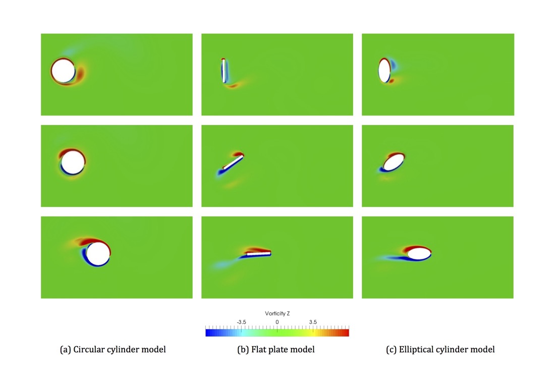
4.3.1. Circular Cylinder Model
The flow field around the circular cylinder model is illustrated in terms of spanwise vorticity and can be seen in Figure 9. At the beginning of the stroke, we notice a mix of counter-clockwise vorticity in red and clockwise vorticity in blue created during the previous stroke. From 0.5 to 1 second, shear vorticity is created above and under the cylinder and a vortex is detect on the upper left of the cylinder. It indicates that the flow above the cylinder is slower than the flow under the cylinder, which causes the vortex to be created where both flows meet. This phenomenon induces an inverse Magnus effect and produce negative lift. During this moment, the unsteady nature of the motion was observed in the profile of lift force. Since the cylinder is rotating clockwise while translating to the right at this moment, a negative lift would be generated due to an inverse Magnus effect. However, as seen sin Figure 8(c), the lift force becomes negative only after around about 1.5 seconds. Indeed, the cylinder is at this moment, still subject to the previous Magnus effect, may be due to the added-mass effect occurring with the previous deceleration of the wing.
From 0.5 to 1 seconds, the rotational velocity decreases and the shear vorticity slowly gets detached and swipes away. However, it is also at this moment that the inverse Magnus effect plays on the lift generation. This one decreases and becomes negative. Shear vorticity is created above and under the cylinder and a vortex is detect behind the cylinder. This vortex is located slightly below y=0 mm at 3.5 seconds, it indicates that the flow is faster above the cylinder than under the cylinder and Positive Magnus effect is observed. This phenomenon induces a relative pressure difference and produce lift. As the translational velocity approaches to zero, the strength of shear vorticty fades. On the other hand, the unsteady motion causes an non-zero lift production, still subject to the Magnus effect. The circular cylinder will then go back in order to complete its cycle, and the others afterwards.
4.3.2. Flat Plate Model
The flow field around the flat plate model can be seen in Figure 10. At the beginning of the stroke, we notice again a mix of counter-clockwise vorticity in red and clockwise vorticity in blue due to the previous stroke. After 1 second, a starting vortex in blue is created at the trailing edge. As a response, a bound vortex (counter-clockwise vorticity) in red is created at the leading edge and increases the circulation, and then the lift. The lift force will increase, as shown in Figure 8(a). After 2.5 seconds, this vortex gets slowly detached and is washed away. The lift decreases to the minimum value. Note that it is difficult to fully distinguish the impact of this LEV over the pure translational lift due to the positive angle of attack and the translation motion. However, this leading edge vortex may increase the critical angle of attack when the stall occurs.
While the vorticity is swiped away, the lift will mainly vary according to the translational velocity. At t=3.5 seconds, a counterclockwise vorticity appears at the leading edge and will grow at t=4 seconds. This seems to be the starting vortex created because of the quick supination. This fast rotation breaks the Kutta–Joukowski condition that needs to be re-established. However, we do not notice any bound vortex or clockwise vorticity at the trailing edge. Hence, this one should be responsible of the increase of lift. Indeed, we do not observe any lift production at the end of the stroke. Even if the slightly higher positive lift peak before the end of the stroke, it seems to be not relevant. At t=4.5 seconds, this starting vortex goes away without any trace of a whatsoever bound vortex. While the translation ends, the lift reaches zero and the wing goes back in order to continue its motion.
4.3.3. Elliptical Cylinder Model
The flow field around the elliptical cylinder model can be seen in Figure 11. At the beginning of the stroke, we notice again a mix of counter-clockwise vorticity in red and clockwise vorticity in blue due to the previous stroke. After 1 second, a counterclockwise vorticity is created. But no vortex is detected on the Q criterion graph as seen in Figure 12, and this circulation does not seem to be due to a whatsoever leading edge vortex. The increase of lift might be due, only, to the translational lift. After 2 seconds, this vorticity gets slowly detached and is swiped away. During this moment, the lift mainly varies according to the translational velocity. A peak of lift is noticed at mid-stroke while the translational velocity reaches its maximum. As it was the case at the beginning of the stroke, only shear vorticity is actually created and no trace of starting vortex that would indicate the presence of the Kramer effect is observed. At the end of the stroke, the translational velocity reaches zero and the lift goes down. It actually goes below zero. It might be due the fact that we reach the stall angle but also because of the added-mass effect. Indeed, when the wing decelerates, the fluid seems to go faster than the wing. As consequence, the angle of attack acts as being negative and then produces a negative lift. Finally, the wing goes back in order to continue its motion.
5. Discussions
5.1. The Magnus Effect and the Kramer Effect
5.1.1. The Circular Cylinder Model and Magnus Effect
The circular cylinder model was chosen to be the reference blunt body to observe the Magnus effect. Even if, due to quasi-steady or unsteady effects, the lift appears to be offset by about 1.6 seconds from the expected trend, we do notice the Magnus effect. Indeed, according to the translation and rotation motion, we would expect the lift to be first negative. However, this one increases first, with even a positive lift of about 6 mN at the beginning of the stroke. The general lift trend is actually well predicted, offset by about 0.6 seconds, by the Kutta-Joukowskitheorem and it makes sense with the PIV results. The maximum lift is reached 0.4 seconds after the supination and the pronation and is 20 percent higher than the Kutta-Joukowski lift prediction. On the other hand, the minimum peak is reached 0.5 seconds after mid-stroke and is twice lower than the Kutta-Joukowski prediction.
5.1.2. The Flat Plate Model and Kramer Effect
It is actually difficult to notice the presence of the Kramer effect for the flat plate model. Indeed, in the direct force measurement, the lift follows essentially the expecting translational lift and other important effects such as wake-capture or added-mass effects interfere with the rotational lift we try to focus on. If we take a look at the qualitative PIV results and computational results, we do notice a starting vortex created at the end of the stroke, when the Kutta-Joukowski condition needs to be re established. However, we do not observe any trace of a whatsoever bound vortex that is supposed to increase the circulation and then the lift. No additional circulation is actually observed at the end of the stroke on Figure 13(b). The Kutta-Joukowski theorem predicts a maximum peak of lift 30 percent higher and a minimum one twice lower. However, the general trend fits relatively well. The peaks are offset by less the 0.5 seconds along the all stroke even considering that the velocity used for the Kutta-Joukowski theorem is simply the translational velocity of the wing.
5.1.3. The Elliptical Cylinder Model
The elliptical cylinder model is not blunt enough to behave like the circular cylinder model and then to observe the presence of the Magnus effect. In term of the amplitude or the trend of the graph, the lift production of the elliptical cylinder model has nothing to do with the circular cylinder one. On the other hand, the elliptical cylinder model is not sharp enough to behave like the flat plate model and then to observe the presence of the Kramer effect. The lift responses for the elliptical cylinder model and for the flat plate are pretty similar. However, the elliptical cylinder model produces a maximum peak of lift 20 percent higher and a minimum one 40 percent lower than the flat plate model. The peaks occur almost at the same time, even if two more fluctuations, after 3 and 7.5 seconds, are observed for the flat plate model. The last one is actually significant because it leads the lift to go below zero while it reaches its maximum for the elliptical cylinder model. The problem is that the presence of the translational lift as well as other unsteadiness avoids us to bring out a potential Kramer effect and to clearly bright out the rotational lift origin. Furthermore, it has been said previously that no trace of bound vortex due to the Kramer effect was found, even in the case of the flat plate model. However, neither leading edge vortex at the beginning of the stroke nor starting vortex at the end is observed. From this point of view, the elliptical cylinder model appears to not be sharp enough.
5.2. Comparison of the Three Wing Models
In general, the flow structures around the three different types of wings have been simulated reasonably well by the current computations. Comparison of the results for the circular cylinder model, the flat plate model and for the elliptical cylinder model are shown on Figure 13(a) for the direct force measurement, on Figure 13(b) for the Kutta-Joukowski theorem and on Figure 13(c) for current computation.
The first thing we can observe in these figures is the similarity between the elliptical cylinder model and the flat plate model compare to the circular cylinder model. So, of course, translational lift occurs in both cases and, coupled with the added-mass effect occurring during the previous deceleration, causes a negative lift at the beginning of the stroke. Significant lift amplitude is observed for the circular cylinder model when compared with the other two models. Indeed, the maximum lift produces by the circular cylinder model is about 3 times higher than the maximum lift produced by the flat plate model and about twice higher than the one produced by the elliptical cylinder model. However, the minimum lift noticed for the circular cylinder model is as low as for the elliptical cylinder model and even higher than for the flat plate model.
Regarding the phase averaged lift, the circular cylinder model produces 4.8 times more lift then the flat plate model but the section lift coefficient remains 2.08 times lower due to the thin thickness of the flat plate.
6. Conclusions
In order to better understand the impact of the supination and the pronation on the total lift production occurring at the end of the stroke while small insects flap their wings, the following experiment and computation have been performed. Using the Reynolds number of a bumblebee, simplified sinusoidal translational and rotational velocity profiles have been chosen. The focus has been held on the rotational lift such that 3 wing profile sections have been studied. A circular cylinder model as the reference of a blunt body for which, hopefully, the well- known Magnus effect will occur, a flat plate model as the reference of a sharp body for which, hopefully, the so called Kramer effect will occur and finally, an elliptical cylinder model, as a transition case. Direct force measurement and particle image velocimetry experiment have been conducted in order to obtain quantitatively the lift produced and to bring out the surrounding flow structure. Moreover, under some assumptions, the KuttaJoukowski theorem has been applied on the PIV results in order to predict, in a quasi steady state point of view, the lift production. The experimental results have been presented with the corresponding computational results. In general there is good agreement between the experimental and computational results.
For the circular cylinder model, the Magnus effect is actually well predicted by the Kutta-Joukowski theorem and it makes sense with the PIV results, with the presence of opposite shear vorticity under and above the cylinder. For the flat plate model, it is actually difficult to notice the presence of the Kramer effect. According to the PIV and computational results, the leading edge vortex is noticed after 0.5seconds (t̂ = 0.11) at the beginning of the stroke. At the end of the stroke, when the Kutta-Joukowski condition needs to be re-established, the creation of a starting vortex is observed after 3.5 seconds (t̂ = 0.76) but no trace of bound vortex due to the Kramer effect is observable. The Kramer effect seems to not be involved in the rotational lift production even if the Kutta-Joukowski conditions appears to be well re-established.
For the elliptical cylinder model, the lift response for the elliptical cylinder model and for the flat plate are pretty similar but it also makes sense according to the presence of the translational lift. However, neither leading edge vortex at the beginning of the stroke nor starting vortex at the end of the stroke is observed. Furthermore, as for the flat plate model, no trace of bound vortex due to the Kramer effect is found. From this point of view, the elliptical cylinder model appears not to be sharp enough to leads the Kutta-Joukowski condition to be re-established. Finally, it is important to note that interference remains that prevent to properly analyze the origin of the lift production for the flat plate and the elliptical cylinder model. Indeed, the presence of the translational lift as well as other unsteadiness avoids us to bring out a potential Kramer effect and to clearly bright out the rotational lift origin.
Author Contributions
Conceptualization, S.O. and S.V.; methodology, S.V. and M.H.W.K.; software, M.H.W.K.; validation, S.O., S.V. and M.H.W.K.; formal analysis, S.V. and M.H.W.K.; investigation, S.V. and M.H.W.K.; resources, S.V. and M.H.W.K.; data curation, S.V. and M.H.W.K.; writing—original draft preparation, M.H.W.K.; writing—review and editing, S.O.; visualization, S.O.; supervision, S.O.; project administration, S.O.; funding acquisition, S.O. All authors have read and agreed to the published version of the manuscript.
Funding
This research was funded by Keio University.
Institutional Review Board Statement
Not applicable.
Informed Consent Statement
Not applicable.
Data Availability Statement
Please contact the corresponding author for the data presented in this paper.
Acknowledgments
The first author would like to thank Keio University for funding the research and AUN/SEED-Net JICA for funding her study at Keio University.
Conflicts of Interest
The authors declare no conflicts of interest.
Abbreviations
The following abbreviations are used in this manuscript:
| PIV | Particle image velocimetry |
| UAV’s | Unmanned air vehicles |
| BAV’s | Bio-mimetic air vehicles |
| LEV | Leading edge vortex |
| AoA | Angle of attack |
| CFD | Computational fluid dynamic |
| PISO | Pressure Implicit with Splitting of Operator |
References
- Ellington, CP. The novel aerodynamics of insect flight: applications to micro-air vehicles. Journal of Experimental Biology 1999, 202, 3439–48. [Google Scholar] [CrossRef] [PubMed]
- Hope DK, DeLuca AM, O’Hara RP. Investigation into Reynolds number effects on a biomimetic flapping wing. International Journal of Micro Air Vehicles 2018, 10, 106–22. [Google Scholar] [CrossRef]
- Shyy W, Aono H, Kang CK, Liu H. An introduction to flapping wing aerodynamics. Cambridge University Press; 2013 Aug 19.
- Dickinson MH, Götz KG. Unsteady aerodynamic performance of model wings at low Reynolds numbers. Journal of Experimental Biology 1993, 174, 45–64. [Google Scholar] [CrossRef]
- Cleaver D, Wang Z, Gursul I. Delay of stall by small amplitude airfoil oscillations at low Reynolds numbers. In 47th AIAA aerospace sciences meeting including the new horizons forum and aerospace exposition 2009 Jan (p. 392).
- Birch JM, Dickinson MH. The influence of wing–wake interactions on the production of aerodynamic forces in flapping flight. Journal of Experimental Biology 2003, 206, 2257–72. [Google Scholar] [CrossRef] [PubMed]
- Yan X, Zhu S, Su Z, Zhang H. Added mass effect and an extended unsteady blade element model of insect hovering. Journal of Bionic Engineering 2011, 8, 387–394. [Google Scholar] [CrossRef]
- Sane SP, Dickinson MH. The aerodynamic effects of wing rotation and a revised quasi-steady model of flapping flight. Journal of Experimental Biology 2002, 205, 1087–1096. [Google Scholar] [CrossRef] [PubMed]
- Dickinson MH, Lehmann FO, Sane SP. Wing rotation and the aerodynamic basis of insect flight. Science 1999, 284, 1954–1960. [Google Scholar] [CrossRef] [PubMed]
- Sun M, Tang J. Unsteady aerodynamic force generation by a model fruit fly wing in flapping motion. Journal of Experimental Biology 2002, 205, 55–70. [Google Scholar] [CrossRef] [PubMed]
- Sun M, Tang J. Lift and power requirements of hovering flight in Drosophila virilis. Journal of Experimental Biology 2002, 205, 2413–2427. [Google Scholar] [CrossRef] [PubMed]
- Shyy W, Aono H, Chimakurthi SK, Trizila P, Kang CK, Cesnik CE, Liu H. Recent progress in flapping wing aerodynamics and aeroelasticity. Progress in Aerospace Sciences 2010, 46, 284–327. [Google Scholar] [CrossRef]
- Sane, SP. The aerodynamics of insect flight. Journal of Experimental Biology 2003, 206, 4191–4208. [Google Scholar] [CrossRef] [PubMed]
- Dickinson MH, Götz KG. The wake dynamics and flight forces of the fruit fly Drosophila melanogaster. Journal of Experimental Biology 1996, 199, 2085–2104. [Google Scholar] [CrossRef] [PubMed]
- Dickinson MH, Lehmann FO, Götz KG. The active control of wing rotation by Drosophila. Journal of Experimental Biology 1993, 182, 173–89. [Google Scholar] [CrossRef] [PubMed]
- Seifert, J. A review of the Magnus effect in aeronautics. Progress in Aerospace Sciences. 2012, 55, 17–45. [Google Scholar] [CrossRef]
- Crall JD, Ravi S, Mountcastle AM, Combes SA. Bumblebee flight performance in cluttered environments: effects of obstacle orientation, body size and acceleration. The Journal of Experimental Biology 2015, 218, 2728–37. [Google Scholar] [CrossRef] [PubMed]
- Willmott AP, Ellington CP. The mechanics of flight in the hawkmoth Manducasexta I. Kinematics of hovering and forward flight. Journal of Experimental Biology 1997, 200, 2705–22. [Google Scholar]
- Baranyi, L. Lift and drag evaluation in translating and rotating non-inertial systems. Journal of Fluids and Structures 2005, 20, 25–34. [Google Scholar] [CrossRef]
- Tokumaru PT, Dimotakis PE. The lift of a cylinder executing rotary motions in a uniform flow. Journal of Fluid Mechanics 1993, 255, 1–0. [Google Scholar] [CrossRef]
- Verboomen, S. Experimental study of rotational lift production under insect flapping wing conditions for different wing section profiles. Master Thesis, Graduate School of Science and Technology, Keio University, Japan, September 2018. [Google Scholar]
- Swanson T, Isaac K. Aerodynamics of Flapping and Plunging Wings using Particle Image Velocimetry Measurements. In 47th AIAA Aerospace Sciences Meeting including The New Horizons Forum and Aerospace Exposition 2009 (p. 1271.
- Stalnov O, Ben-Gida H, Kirchhefer AJ, Guglielmo CG, Kopp GA, Liberzon A, Gurka R. On the estimation of time dependent lift of a European starling (Sturnus vulgaris) during flapping flight. PLoS One 2015, 10, e0134582. [Google Scholar]
- Noca, F. On the evaluation of time-dependent fluid-dynamic forces on bluff bodies. California Institute of Technology; 1997. [Google Scholar]
- Krish P Thiagarajan and Armin W Troesch. On the use of various contour shapes for evaluating circulation from PIV data, 13th Australasian Fluid Mechanics Conference, Monash University, 1998.
Figure 1.
Experimental set-up.
Figure 2.
(a) Translation distance assumption; (b) Definition of the coordinates.
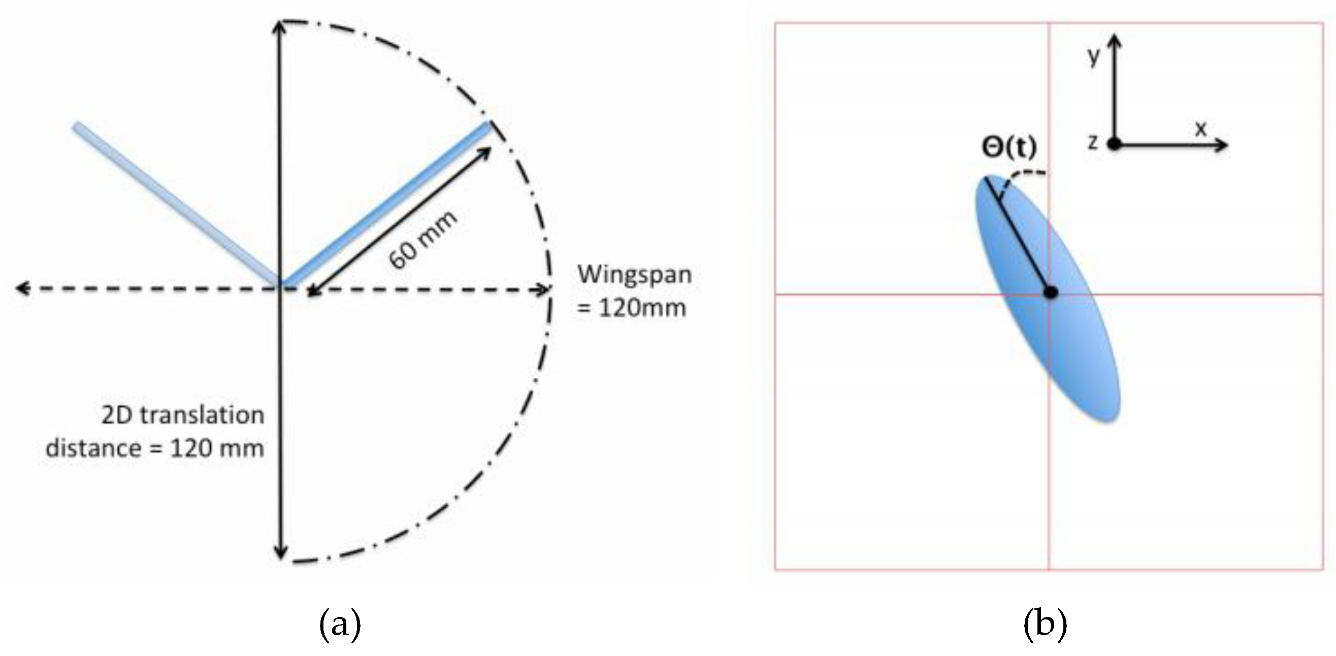
Figure 3.
Wing position along the whole stroke.
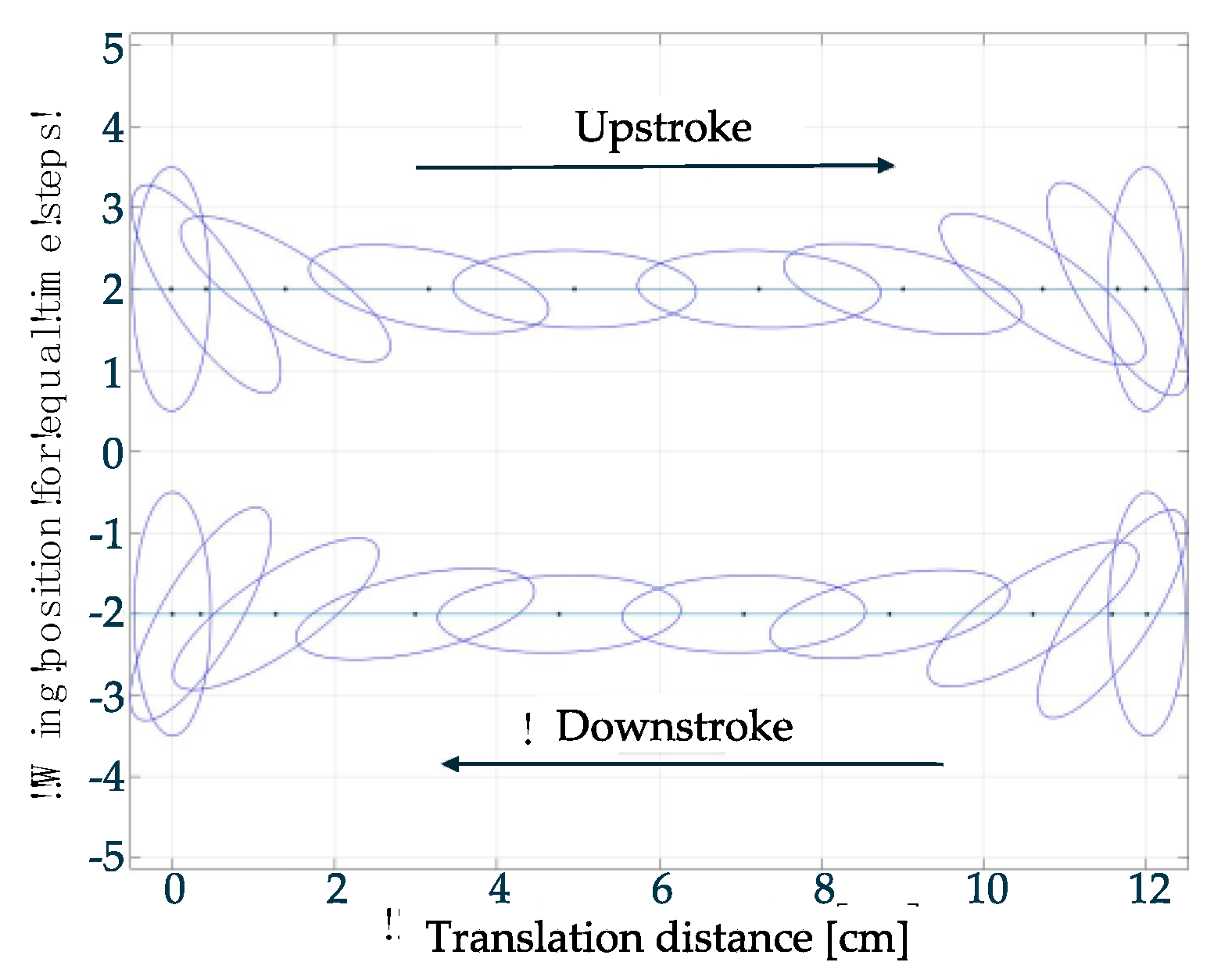
Figure 4.
(a) Water tank configuration; (b) Wing location inside the water tank.
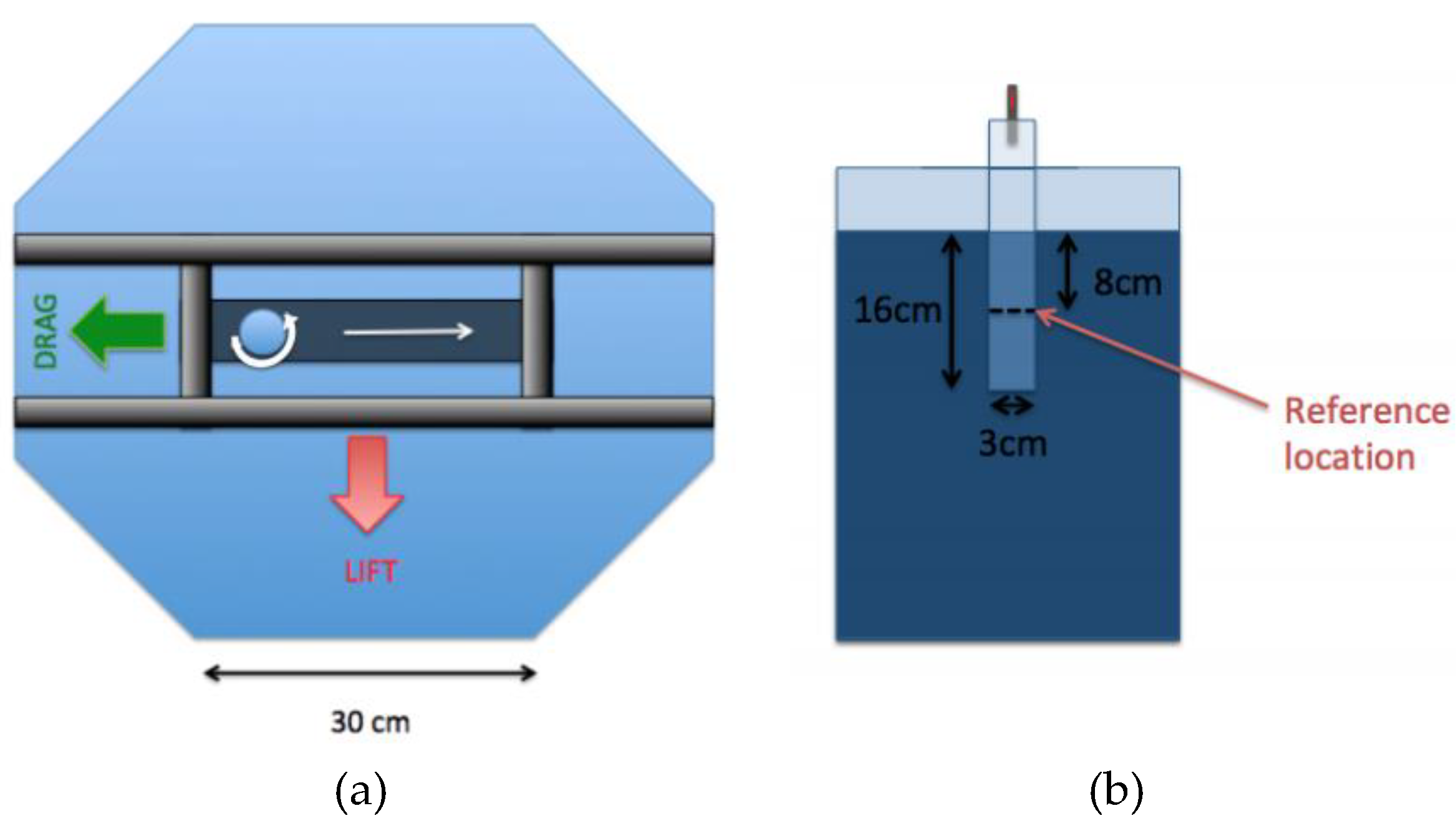
Figure 5.
(a) Side view; (b) Upper view of the 3-wing models. A: The flat plate model. B: The circular cylinder model. C: The elliptical cylinder model.
Figure 5.
(a) Side view; (b) Upper view of the 3-wing models. A: The flat plate model. B: The circular cylinder model. C: The elliptical cylinder model.
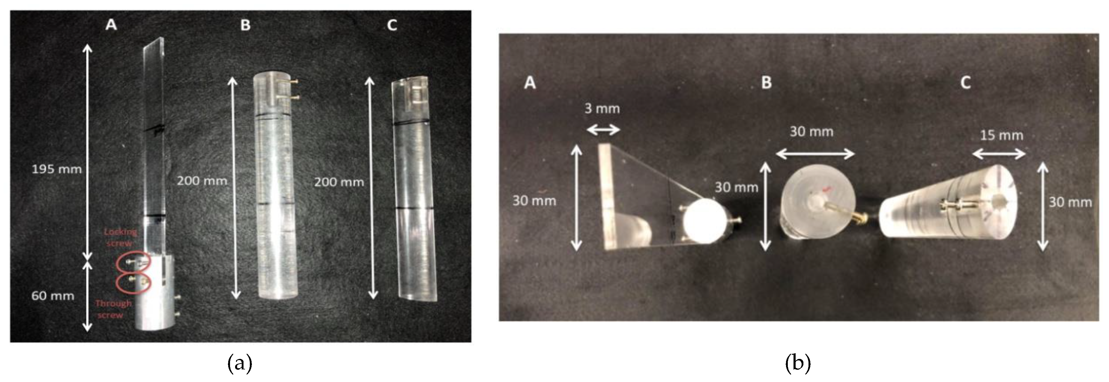
Figure 6.
(a) Brass axis connecting the wing to the stepping motor with the strain gaugesfixed on it; (b) Strain- gauges configuration.
Figure 6.
(a) Brass axis connecting the wing to the stepping motor with the strain gaugesfixed on it; (b) Strain- gauges configuration.
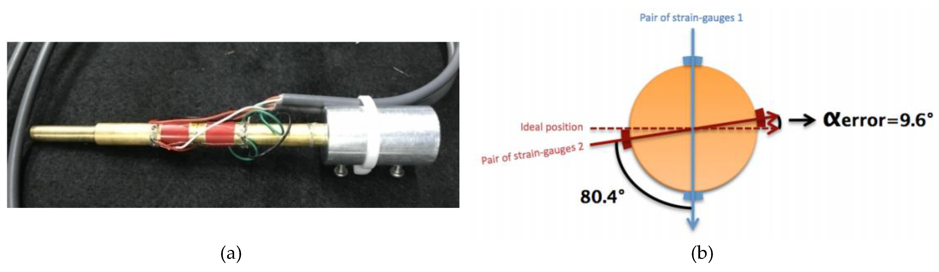
Figure 7.
(a) Side view of the particle image velocimetry set-up; (b) Upper view of the particle image velocimetry set-up.
Figure 7.
(a) Side view of the particle image velocimetry set-up; (b) Upper view of the particle image velocimetry set-up.
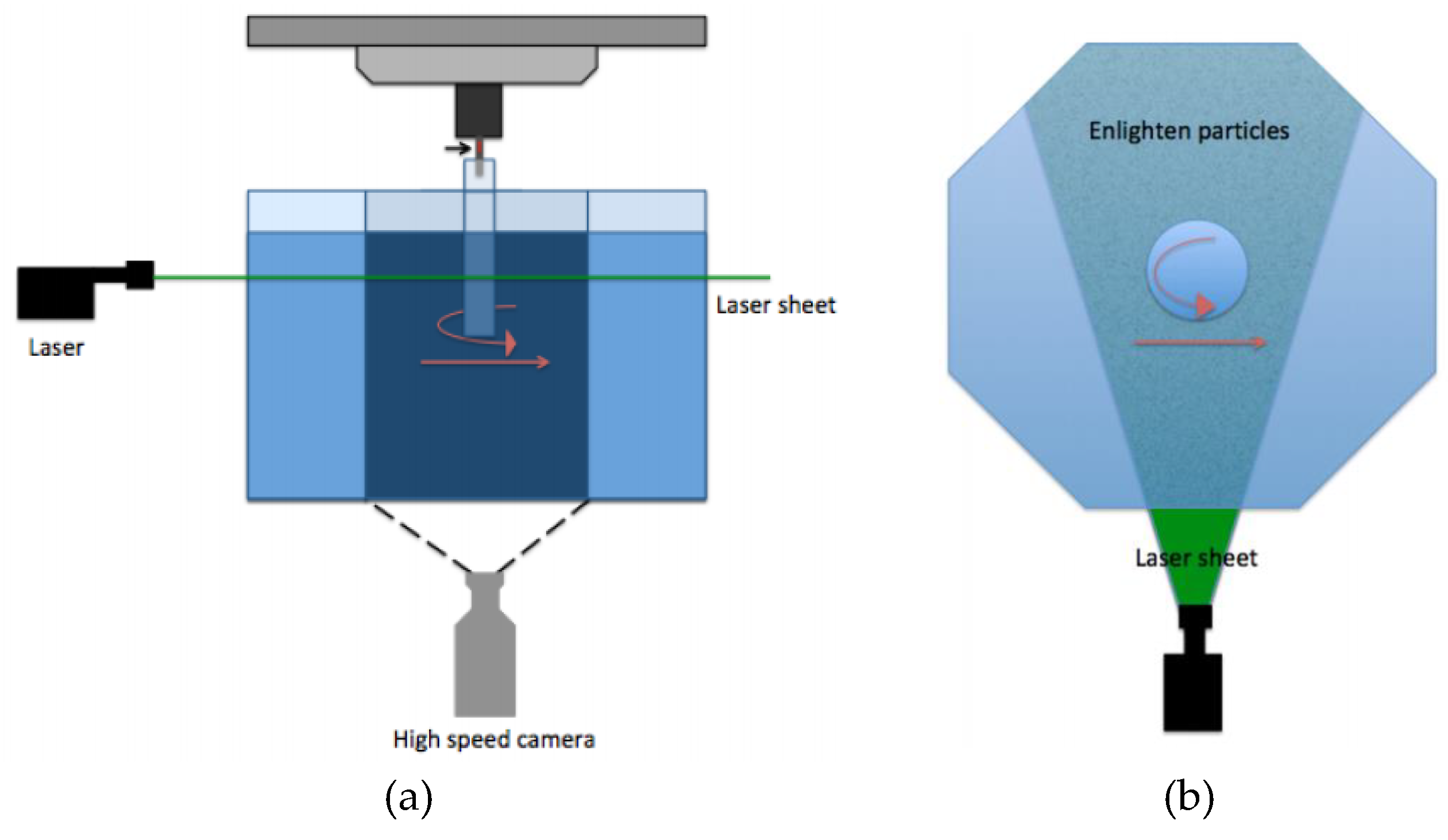
Figure 8.
Lift measurement and prediction of Samuel et al. [20] for: (a) Flat plate; (b) Elliptical cylinder; (c) Circular cylinder model. Red = experimental measurements. Green = Kutta-Joukowski prediction. Present computational results for: (d) Flat plate; (e) Elliptical cylinder; (f) Circular cylinder model.
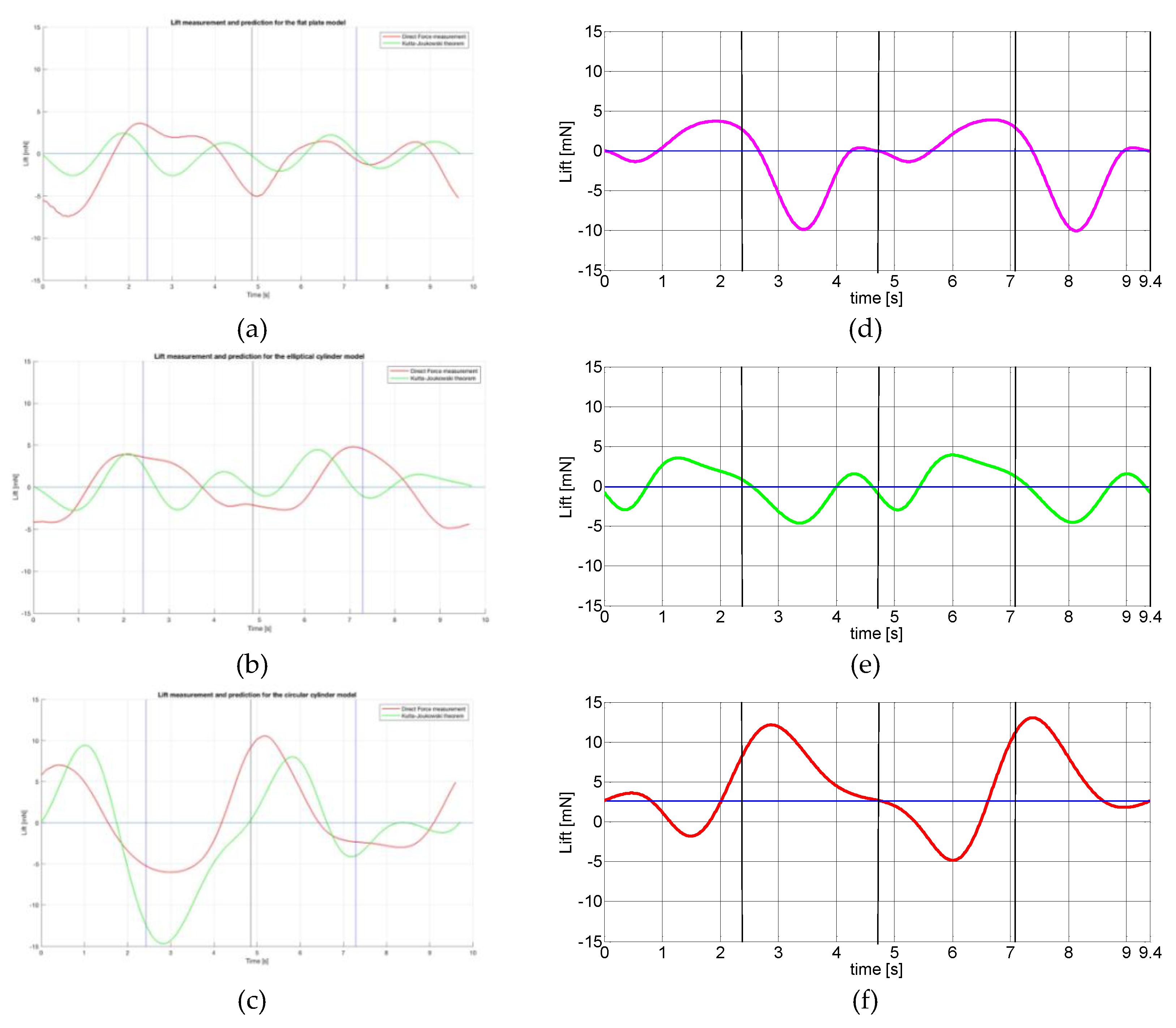
Figure 9.
Vorticity field for circular cylinder model; (a) PIV results and (b) Computational results.
Figure 9.
Vorticity field for circular cylinder model; (a) PIV results and (b) Computational results.
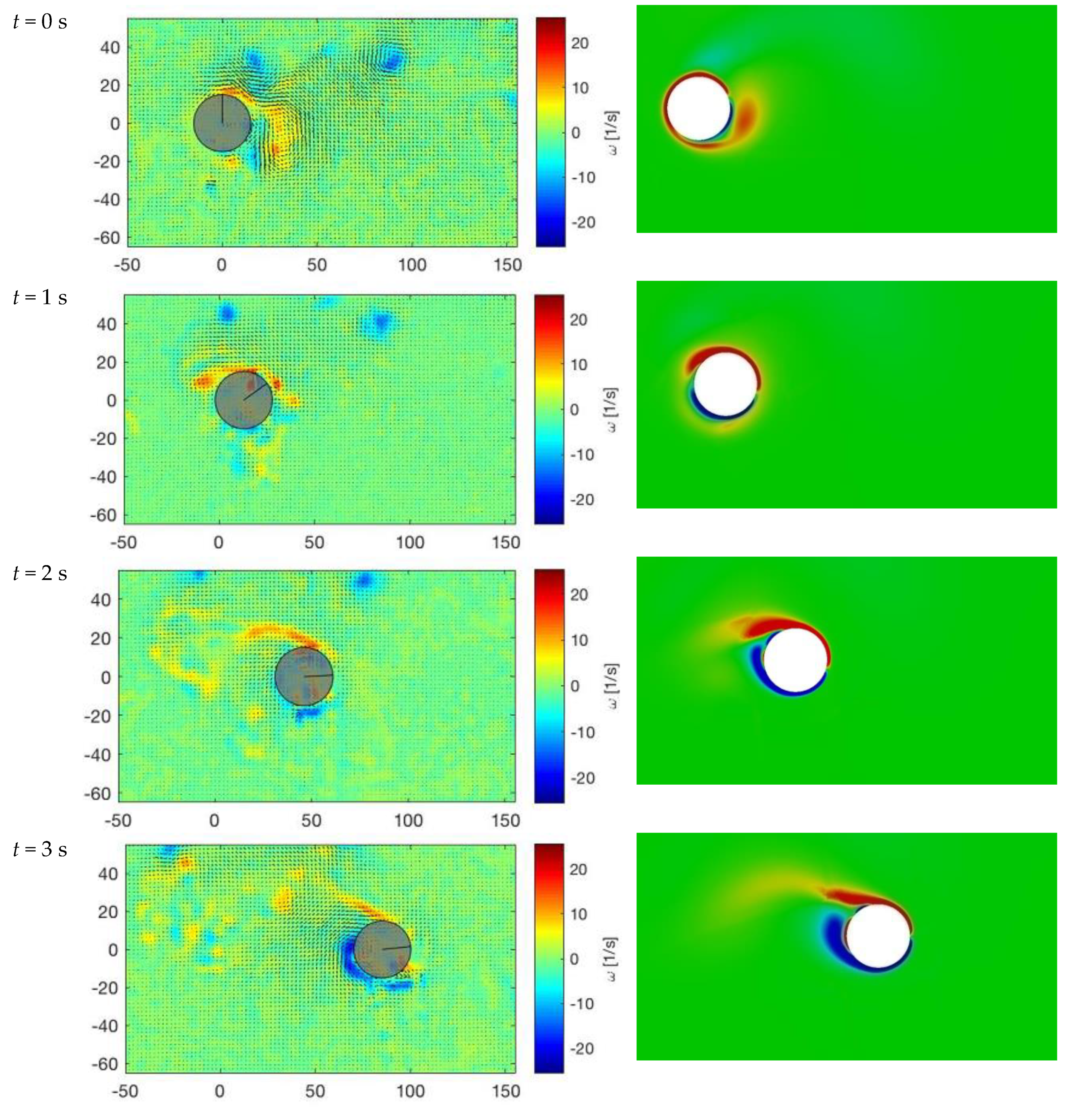
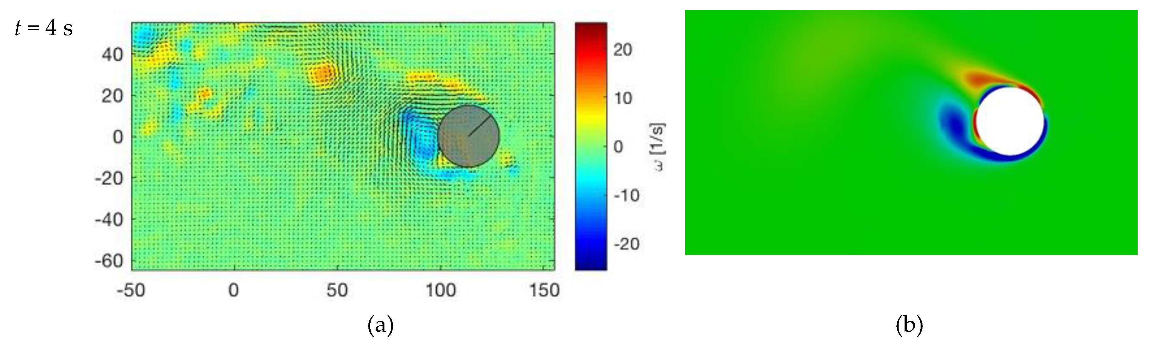
Figure 10.
Vorticity field for flat plate model; (a) PIV results and (b) Computational results.
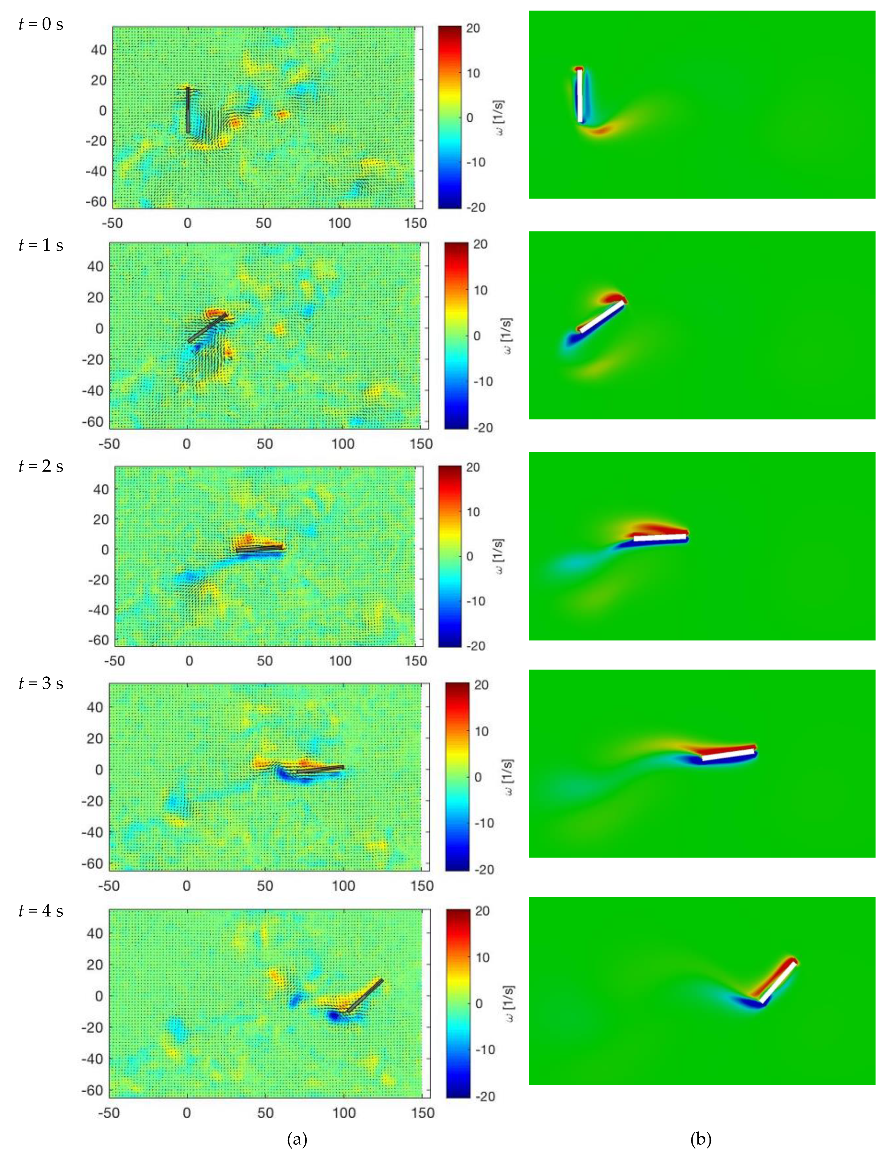
Figure 11.
Vorticity field for elliptical cylinder model; (a) PIV results and (b) Computational results.
Figure 11.
Vorticity field for elliptical cylinder model; (a) PIV results and (b) Computational results.
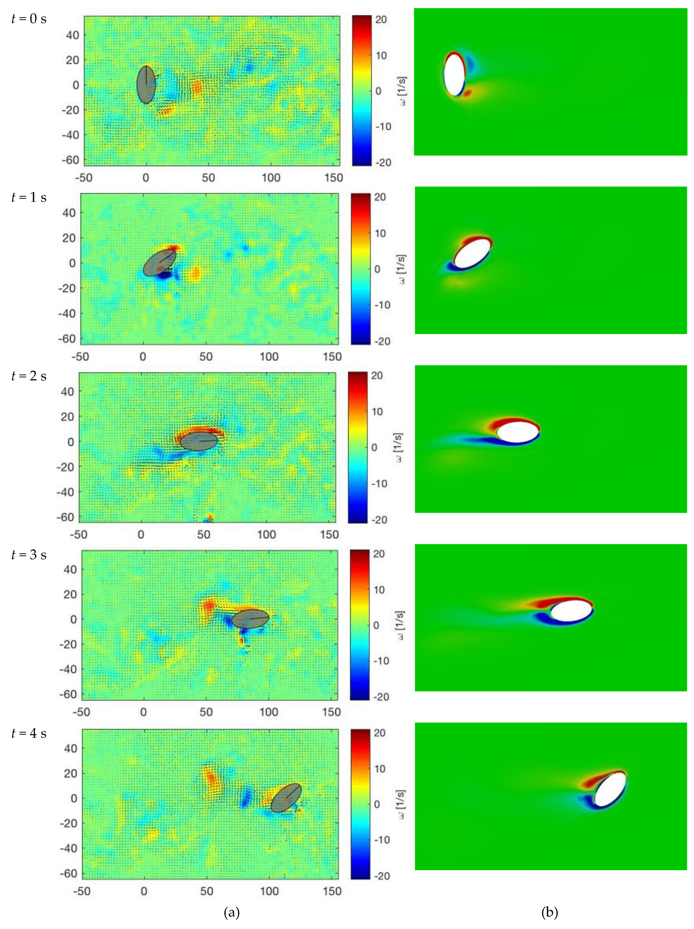
Figure 12.
Q criterion for elliptical cylinder model; (a) PIV results and (b) computational results.
Figure 12.
Q criterion for elliptical cylinder model; (a) PIV results and (b) computational results.
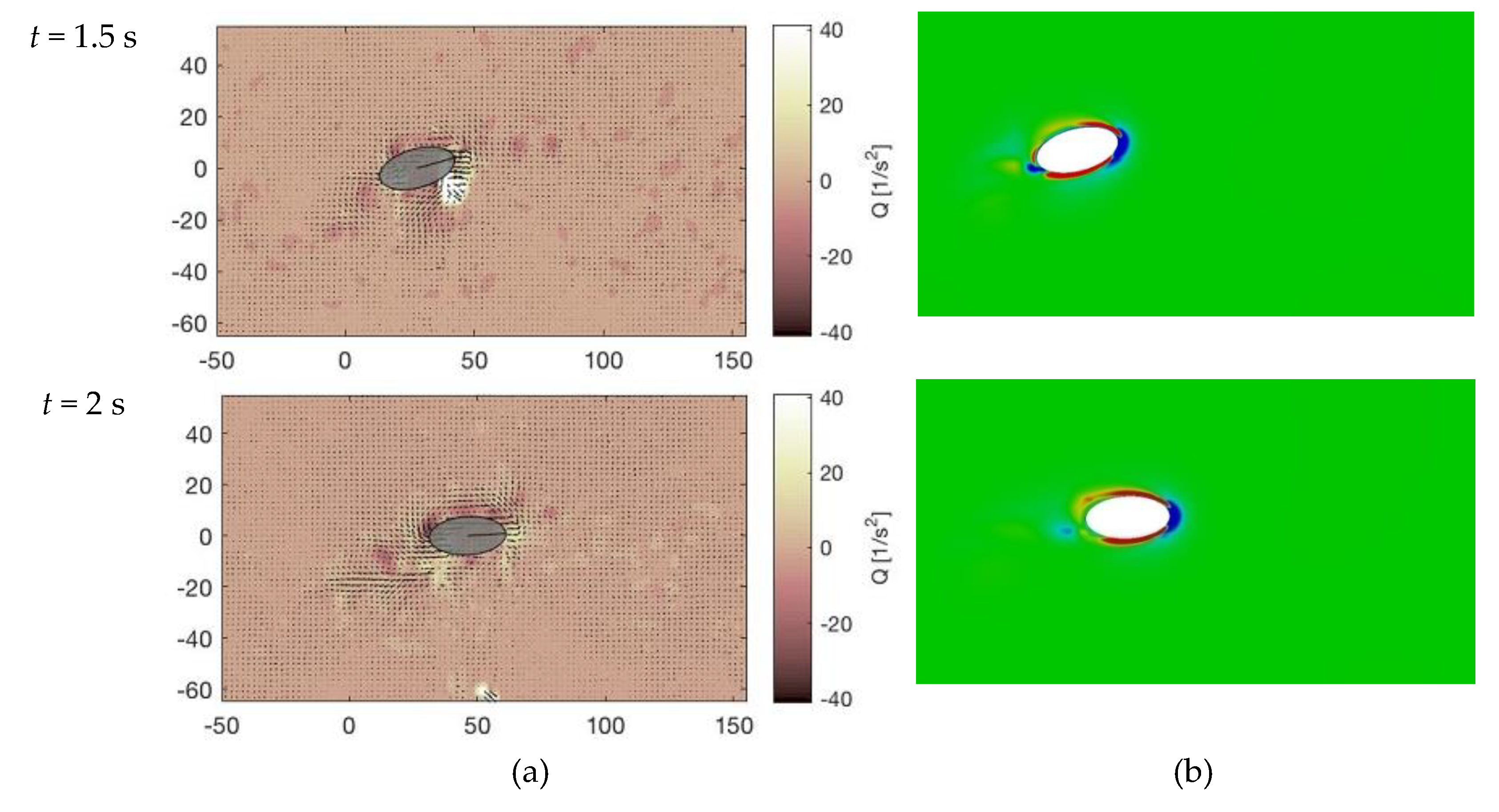
Figure 13.
(a) Direct force measurement; (b) Kutta-Joukowski theorem; (c) Computational results for all the wing models.
Figure 13.
(a) Direct force measurement; (b) Kutta-Joukowski theorem; (c) Computational results for all the wing models.
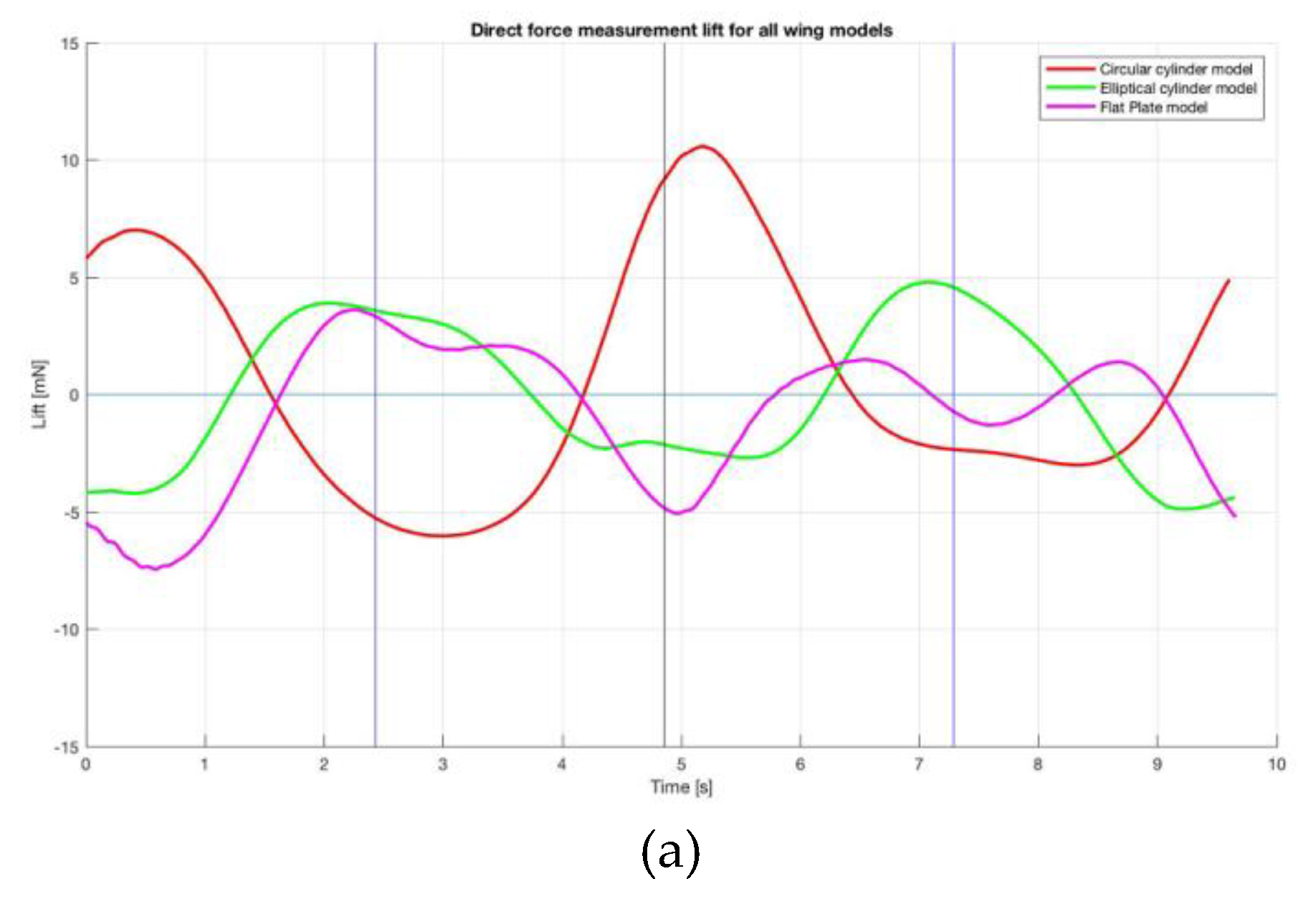
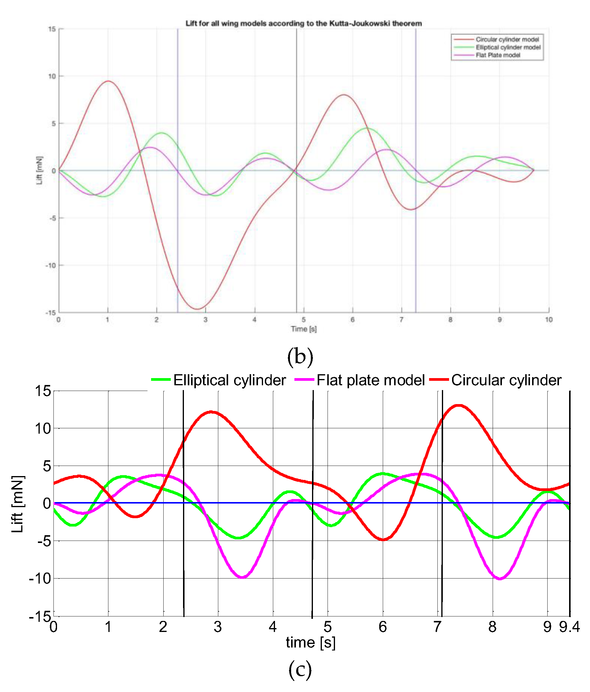

Table 1.
PIV equipment specifications.
| Laser | Tracer particles | High speed camera | Lens |
|---|---|---|---|
| Nd : YAG Laser | Nylon 12 (5g) | Photoron Fastcam SA3 (60 frames per second) | Micro-Nikkor 55 mm f / 2.8 |
Table 2.
Numerical schemes.
| Numerical schemes | Used option |
|---|---|
| ddtSchemes | Euler |
| gradSchemes | Gauss linear |
| divSchemes | Gauss upwind |
| interpolationSchemes | Linear |
| snGradSchemes | Limited 0.5 |
Disclaimer/Publisher’s Note: The statements, opinions and data contained in all publications are solely those of the individual author(s) and contributor(s) and not of MDPI and/or the editor(s). MDPI and/or the editor(s) disclaim responsibility for any injury to people or property resulting from any ideas, methods, instructions or products referred to in the content. |
© 2025 by the authors. Licensee MDPI, Basel, Switzerland. This article is an open access article distributed under the terms and conditions of the Creative Commons Attribution (CC BY) license (http://creativecommons.org/licenses/by/4.0/).
Copyright: This open access article is published under a Creative Commons CC BY 4.0 license, which permit the free download, distribution, and reuse, provided that the author and preprint are cited in any reuse.


