Submitted:
31 July 2025
Posted:
01 August 2025
You are already at the latest version
Abstract
Alzheimer’s disease is a neuro-degenerative disorder that severely affects the global elderly population,early and accurate diagnosis plays an important role in developing effective treatment options and slowing disease progression.In this study, we introduce a novel deep learning framework, termed Wavelet Transform-based Residual Gated Attention Network (WTRGANet). This model integrates wavelet transform with a residual gated attention mechanism to enhance feature extraction. It is specifically designed for multi-class classification of Alzheimer’s disease using MRI images.WTRGANet Multi-Resolution Feature Extraction by Integrating Wavelet Transforms,expanded receptive field and enhanced response to low-frequency information. At the same time, the model introduces a residual gated attention module, which combines the channel attention and spatial attention mechanisms to dynamically optimise the feature representation and improve the model’s attention to key features.In addition, ablation experiments verified the critical contribution of the wavelet transform convolutional layer and the residual gated attention module to the model performance, with the removal of either module leading to a significant degradation in performance.
Keywords:
Alzheimer’s disease
; MRI pictures
; WTRGANet
; residual gated attention module
; wavelet transformation
; channel attention
; spatial attention
1. Introduction
Immediately after the aging population has been affected, the disease of the dimer is a progressive neurodegenerative disease that has a major effect on the general public. As a result, cognitive function and severe memory impairment gradually deteriorate [1]. Since people of all countries have grown older than the general population, the prevalence of Alzheimer’s disease is increasing and putting a lot of strain on families and public health systems [2]. Early diagnosis of the condition of Alzheimer disease is a crucial component of both accurate and early diagnosis. The use of magnetic resonance imaging (MRI) to diagnose Alzheimer’s disease has grown to be an ineffective instrument. MRI not only gives doctors a high-resolution image of brain structures but also helps them see small brain abnormalities [3]. Nonetheless, there are still many problems with the accurate identification of Alzheimer’s disease based on MRI images. The primary causes of these difficulties are the morphological and structural variety of images at different phases of the disease process as well as the subtle differences between focal areas and normal brain tissue, which makes accurate classification by standard image processing and manual analysis methods very challenging and a daunting task even for experienced radiologists [4,5]. In the area of medicine image analysis in recent years, deep learning approaches have shown amazing advances in the field of image processing, which has greatly improved the ability to processes, interpreting, and categorizing medical images with increased accuracy and efficiency thanks to these breakthroughs. And have shown to be very helpful in image recognition and feature extractio [6]. .However, although many studies have attempted to diagnose Alzheimer’s disease using deep learning models, there is still room for improvement in processing multi-resolution features of images and enhancing the accuracy of the models [7]. Conventional Convolutional Neural Networks perform well in extracting local features, but often ignore global contextual information and complex spatial relationships. In addition, the common noise and blurring phenomena in MRI images further increase the difficulty of recognition [8]. To overcome these challenges, this study proposes a deep learning model called WTRGANet, which aims to improve the recognition performance of Alzheimer’s disease MRI images by integrating Wavelet Transform and Residual Gated Attention mechanisms. Specifically, WTRGANet combines the multi-resolution feature extraction capability of the Wavelet Transform with the efficient feature learning capability of the Residual Network, while introducing the Gated Attention module to enhance the channel and spatial feature representation.
The main contributions made by this study as follows:
The goal is to use the wavelet transform, which is the residual gated attention mechanism, as part of the deep learning model to recognize MRI pictures of ADMs in multiple categories.
The input image is divided into many frequency parts by the process of wavelet decomposition, and the smaller convolutional kernel operations are carried out every frequency, after which inverse wavelet reconstruction is used to produce an improved output that increases the receptive field and increases the reaction ability of low-frequency information, which is the result of this process. Combined with the remaining mechanism in place and the spatial attention mechanism, to combine the two methods, so as to build the remaining gated attention module and realize the spatial attention mechanism of the whole channel. Compared with the classic non-local attention mechanism, the RGA module not only increases the image blurring and the noise resistance of the model, but also keeps the high efficiency.
The overall performance was verified using ablation experiments after WTRGET was extensively assessed by a number of performance indicators as well as the contribution of each of the different components to the total performance.
This section of the work includes the following: The second part covers related research, as well as the theoretical background; and introduces the methods and approaches that are currently in place for the MRI image identification of Alzheimer’s disease. The WTRGANet model is described in detail in Section III, which is part of the process. The experimental results are displayed in Part IV, which also gives us a detailed analysis of the model performance. The research, limitations, and possible research directions are all covered in Part V, which also covers the study’s importance.
2. Related Works
Traditional machine learning approaches are still dominant in classification tasks in AD, with support vector machines being one of the most common classifiers.Ramírez et al. proposed a continuous support vector machine model approach, which utilises voxel values as features for classificatio [7]. This method demonstrated superior classification results to traditional local statistical parameter mapping (SPM) methods without relying on pathological knowledge. On the other hand Magnin et al. used SVM to extract grey matter features on 3D T1-weighted MRI images and combined it with bootstrap resampling technique to enhance the robustness of the classification results [8]. Segovia et al. studied SPECT images to further improve the accuracy of early diagnosis of AD by optimising the classification effect of SVM through feature selection and standardised mean square error feature extraction [9]. To further improve the classification performance, researchers have used more sophisticated feature extraction and dimensionality reduction methods.For example, Ramírez et al. combined kernel principal component analysis and kernel linear discriminant analysis for dimensionality reduction of functional MRI images and used SVM for classification, achieving significant accuracy improvements [10]. Oliveira et al. investigated changes in cortical thickness in AD patients and combined cortical and volumetric data for automatic classification, showing that training SVMs using volumetric information about grey matter, white matter and subcortical structures outperforms methods using only cortical thickness [11]. With the advancement of deep learning techniques, there has been a shift from traditional machine learning to deep neural networks for classification tasks in AD.Hon et al. used a migration learning approach to train a pre-trained model on the OASIS MRI dataset, adjusting only the fully-connected layer to improve performance on a small dataset [12]. Liu et al. proposed a deep learning framework for fusing multimodal neuroimaging features, a model that extracts complementary information through a zero-masking strategy and achieves superior results in both binary and multiclassification tasks in AD [13]. In addition, in terms of model optimisation, Venugopalan et al. proposed a feature extraction method based on superimposed denoising autoencoder and combined it with 3D convolutional neural network to process the MRI images, which achieved classification results superior to those of the traditional machine learning models [14]. Abrol et al., on the other hand, employed a deep learning-based Granger causality estimator to model brain connectivity. They further integrated this approach with a Long Short-Term Memory network to analyze dynamic time-series data, thereby enhancing the accuracy of Alzheimer’s disease diagnosis [15].
In the field of medical image analysis, Wavelet transform is extensively employed to improve the effectiveness of feature extraction by capturing multi-scale spatial and frequency information.The wavelet transform can effectively decompose the different frequency components of an image, enabling the model to learn a richer representation of the features.It has been shown that combining wavelet transform with deep learning can effectively improve model robustness and classification performance [16]. In addition, attention mechanisms are increasingly used in image classification tasks. The channel attention mechanism adaptively adjusts the weights of different channels in the feature map, enhancing the representation of important features. Meanwhile, the spatial attention mechanism directs the model’s focus toward key regions, thereby improving classification accuracy [17]. Although deep learning methods have shown great potential for classification tasks in AD, some challenges remain. For example, the problem of category imbalance in MRI datasets, researchers are gradually adopting synthetic minority over-sampling techniques or data enhancement methods to solve this problem . In addition, as deep learning models require high dataset size and quality, how to standardise the datasets and improve the generalisation ability of the models is still a challenge to be addressed.

Table 1.
Literature evaluation of numerous recent cutting-edge approaches used in AD detection and classification.
Table 1.
Literature evaluation of numerous recent cutting-edge approaches used in AD detection and classification.
| Approach | Year | Method | Results Accuracy |
Imbalance Handling |
|---|---|---|---|---|
| Ramírez et al. | 2013 | Continuous Support Vector Machines | None | |
| Magnin et al. | 2009 | SVM-based 3D MRI classification | None | |
| Segovia et al. | 2012 | Feature selection and standardized MSE methods | - | None |
| Oliveira Jr. et al. | 2010 | SVM classification of cortical thickness and volume information | 91% | None |
| Hon & Khan | 2017 | Transfer learning | 94.8% | None |
| Liu et al. | 2023 | Deep learning framework for multimodal neuroimaging | 94.8% | None |
| Venugopalan et al. | 2021 | Feature extraction based on denoising autoencoder with 3D-CNN | 93.18% | None |
| Abrol et al. | 2019 | Deep learning-based Granger causality estimator | - | None |
3. Methodology
3.1. Methodological Processes
The WTRGANet method combines the wavelet transform and residual gated attention mechanism with the aim of improving the classification performance of Alzheimer’s disease MRI images. Figure 1 shows the processing flow of the algorithm. Firstly, the input MRI images are resized to 224x224x3 by a preprocessing step and normalised by pixel values in order to fit the input requirements of the neural network. The dataset is divided into a training set (80%) and a test set (20%) and data enhancement techniques (e.g., random level flipping, rotation and colour perturbation) are employed to cope with category imbalance and to improve the generalisation ability of the model.WTRGANet extracts multi-resolution features by integrating the wavelet transform, which enhances the response of the low-frequency information and extends the receptive field to improve the ability to capture the details of the image. The BasicBlock is used for local feature extraction, while the Residual Gated Attention Module combines channel and spatial attention mechanisms to dynamically optimise feature representation and suppress the effects of noise and blur. Eventually, the model is classified by the Fully Connected Layer,which outputs four categories: mildly demented, moderately demented, non-demented, and very mildly demented. The specific algorithm module design is described in detail below.
3.1.1. WTRGANet Network Architecture
The network architecture of the WTRGANet model is shown in Figure 2, combining four core modules: the WTConv2d, BasicBlock, RGABlock, and DenseBlock, each of which plays an important role at different stages of the network and works in concert to achieve improved recognition of MRI images of Alzheimer’s disease.First, the WTConv2d module serves as an input layer containing a convolutional layer and a wavelet transform convolutional layer.The standard convolutional layer is used to extract the initial features of the image, while the wavelet transform convolutional layer enhances the responsiveness of the low frequency information by performing a multi-resolution decomposition of the image .This module also includes a ScaleModule, which scales the image features to ensure that the different frequency components are efficiently passed on to subsequent layers.The ReduceConv layer further adjusts the dimensionality of the feature map to help the network extract more valuable features.
Next, the four BasicBlock modules, which are used for in-depth processing of the image features, are used to operate with two layers of convolution, each of which is immediately followed by batch normalisation and the ReLU activation function.Through the residual connection, BasicBlock can effectively alleviate the problem of gradient vanishing, and make the information can be better passed to the subsequent layers to improve the expressive ability and training stability of the network.Subsequently, the feature representation is further optimised by the RGA Block (Residual Gated Attention Block) module with the BasicBlock module,Which incorporates the Channel Attention mechanism alongside the Spatial Attention mechanism.
Through adaptive average pooling and convolutional operations, the RGA module assigns weights to each channel and spatial location to strengthen key features and suppress irrelevant features.Next, features are aggregated through a Global Average Pooling layer to further reduce the number of parameters and enhance the representation of global information. The network also introduces a Dropout layer as a means of regularisation, Which randomly deactivates certain neuron activation values to mitigate overfitting and enhance the model’s generalization capability. Finally, The Dense Block module is designed to integrate high-level features within the network, facilitating more effective feature propagation and reuse,mapping the extracted high-level features to the final output layer using the Fully Connected Layer, and outputting a multi-category classification via SoftMax to complete the task of recognising mild, moderate, non-dementia and very mild dementia in Alzheimer’s disease.
Overall, the deep convolutional network backbone of WTRGANet consists of wavelet transform, multiple convolutional layers, residual units, channel attention mechanisms, and spatial attention mechanisms. It can be described as follows: First, the input image undergoes wavelet transform through a custom WTConv2d module, decomposing the image into low-frequency and high-frequency components. The low-frequency components are processed by a standard 7×7 convolutional layer for initial feature extraction, followed by batch normalization and ReLU activation to generate the initial feature map. The high-frequency components are processed by independent depthwise convolutional layers, which use grouped convolution (groups=9) to achieve efficient feature extraction and parameter sharing. Next, the network passes through four main BasicBlock stages. Each BasicBlock consists of two 3×3 convolutional layers, batch normalization layers, and ReLU activation functions, with skip connections adding the input feature map to the output feature map,is formulated as:
WTConv2d The feature maps after wavelet transformation are represented as follows, and the detailed transformation process will be described later. . two convolutional layers and activation functions are represented as follows. X is input feature map, Y is output feature map.At the end of the stage, we integrate the Residual Gated Attention Module to recalibrate the output feature map through channel and spatial attention. Specifically, the RGA_Module dynamically adjusts the weights in the feature map using the following formula:
is channel attention weights, They are generated through global average pooling followed by two convolutional layers. is spatial attention weights, They are generated through a dimensionality-reduction convolution followed by two convolutional layers, ⊙ denotes the element-wise multiplication operation. The channel attention mechanism strengthens the representation of significant channels, whereas the spatial attention mechanism emphasizes crucial features in key spatial regions, collectively improving the model’s discriminative power. As the network depth increases, the number of channels in the feature maps gradually increases to 64, 128 , and 256 , while the spatial dimensions of the feature maps are progressively reduced through convolutional operations with a stride of 2 .Finally, the feature maps processed through all convolutional layers and attention modules are compressed into fixed-size feature vectors via a global average pooling layer:
Subsequently, the feature vectors are mapped to a probability distribution over the target classes through a linear fully connected layer, achieving the final classification output:
and are the weight and bias parameters of the fully connected layer, respectively. The Softmax function transforms the output of the linear layer into a probability distribution over the classes. By integrating wavelet transform and residual gated attention mechanisms, the entire backbone network can dynamically adjust and optimize feature representations at different levels.
3.2. Wavelet Transform Convolutional Layer
In WTRGANet, the WTConv2d module is a core component responsible for multi-resolution feature extraction through wavelet transform. The module first performs wavelet decomposition on the input image, then conducts convolution operations in the wavelet domain, and finally reconstructs the feature maps via inverse wavelet transform. Specifically, the WTConv2d module consists of the following key parts: creation and initialization of wavelet filters, wavelet transform and inverse wavelet transform, basic convolution operations, convolution and scaling of high-frequency components, and feature reconstruction and output.
3.2.1. Creation and Initialisation of Wavelet Filters
The WTConv2d module utilizes Daubechies wavelets (e.g., db1) from the PyWavelets library to create wavelet filters for both forward and inverse transforms.Specifically, the create_wavelet_filter function generates low-pass and high-pass filters , which are defined as follows:
These filters form an orthonormal basis, enabling the wavelet transform and inverse wavelet transform to be implemented through standard convolution and transposed convolution. The low-pass filters are used to capture the main structural information of the image, while the high-pass filters are used to capture details and edge information.
3.2.2. Wavelet Transform (math.)
As shown in Figure 3, during the forward propagation process, the input image X is first decomposed into a low-frequency component and high-frequency components , by the wavelet transform function , whose mathematical expression is as follows:
Conv denotes the depthwise convolution operation with a stride of 2 , achieving downsampling. The low-frequency component retains the main structural information of the image, while the high-frequency component contains details and edge information.
3.2.3. Basic Convolutional Operations
The low-frequency component a undergoes further feature extraction through a standard convolutional layer base_conv. This convolutional layer functions similarly to traditional convolution operations, but since the input features have already undergone multi-resolution processing via wavelet transform, it can more effectively capture the image’s details and structural information. The mathematical expression for the basic convolution operation is as follows:
Here, is the basic convolution kernel, and ScaleModule is a trainable scaling module used to dynamically adjust the scale of the feature maps.
3.2.4. Convolution and Scaling of High Frequency Components
The high-frequency component is processed by a set of independent convolutional layersConv , which employ depth-wise convolution, meaning each input channel is convolved independently. The specific expression is as follows:
is the convolution kernel for the i-level wavelet decomposition, and ScaleModule i is the corresponding scaling module. The processed high-frequency features are dynamically adjusted through the scaling module, further enhancing their representational capability.
3.2.5. Feature Reconstruction and Export
The processed low-frequency and high-frequency features are recombined through the inverse wavelet transform function IWT to reconstruct the enhanced feature map Z. The specific steps are as follows:
- (1)
- The low-frequency component and the high-frequency component are added together to obtain the fused feature map:
- (2)
- The feature maps are reconstructed through the inverse wavelet transform function IWT :
Finally, the output feature map Z combines the main structural features from the low-frequency information and the detailed features from the high-frequency information, forming the final output:
ReduceConv is a convolutional layer used to reduce the number of channels in the high-frequency components to match the output channels, ensuring consistent dimensionality of the feature maps.
As shown in Figure 4, the diagram illustrates an image processing pipeline that combines convolution, wavelet transform, and inverse wavelet transform. First, the original MRI image undergoes convolution operations to extract local features such as edges and textures. Next, wavelet transform is applied to decompose the image into components of different frequencies, capturing low-frequency smooth information and high-frequency detail information separately. Finally, the inverse wavelet transform reconstructs the image from the decomposed components, merging the frequency components to produce an image with enhanced details and structures. Through this multi-level, multi-scale learning process, the model can more effectively extract useful information from the image, improving its ability to understand and process image content.
3.2.6. Theoretical Advantages of WTConv2d
The WTConv2d module demonstrates its theoretical strengths in the following ways:
- (1)
- Multi-resolution feature extraction:With the wavelet transform, WTConv2d is able to capture image features at different frequency levels, both extracting local details and preserving global structural information.
- (2)
- Feel the Wild Expansion:Applying independent small convolutional kernel operations on the high frequency components, WTConv2d effectively extends the receptive field and improves the model’s ability to capture the global information of the image
- (3)
- Parametric efficiency:Using deep convolution, WTConv2d avoids excessive growth in the number of parameters while maintaining efficient feature extraction capability.In concrete terms,Using multi-level wavelet decomposition level WT) The number of parameters increases only linearly as , and the sensory field grows exponentially as . k.
WTConv2d effectively controls the number of parameters and the computational cost by combining the wavelet transform and deep convolution while maintaining the feeling field expansion. The computational costs (FLOPs) of deep convolution can be expressed as:
C is number of input channels, is Spatial dimension of input, is Convolutional kernel size, is stride.For example, for a single-channel input with a spatial size of , the FLOPs for a convolution kernel are 12.8 M , while the FLOPs for a convolution kernel are 252 M .Considering a set of convolutional operations in WTConv2d, each wavelet-domain convolution reduces the spatial dimension by a factor of 2 but increases the number of channels by a factor of 4 . Therefore, its FLOPs count is:
ℓ is wavelet decomposition level,For a input and a 3 -level WTConv, the FLOPs using a convolution kernel are 15.1 M , which still demonstrates a significant advantage compared to the computational cost of standard depthwise convolution ( 17.9 M FLOPs). The WTConv2d module achieves the goals of multi-resolution feature extraction and receptive field expansion by combining wavelet transform with depthwise convolution, while effectively controlling the number of parameters and computational cost.
3.3. Residual Gated Attention Module
Residual Gated Attention Module The role of the residual gated attention module is to allow the model to focus on key information, such as important features. The residual gated attention module is not the same as a static convolution or attention mechanism; the residual gated attention module allows the network to focus on wherever it wants to focus, or it can ignore some unimportant features and focus on only the important ones. The model in this study combines the two mechanisms, the channel attention mechanism and the spatial attention mechanism, and then applies a residual link. In this way, the key information in the feature map can be passed on more efficiently, and the gradient back propagation will not get stuck. Channel attention is responsible for judging ‘those feature channels are more important’, while spatial attention is focusing on ‘that part of the graph is more worthy of attention’. Although these two mechanisms work independently of each other, they have many limitations when used alone. In practice, this design is particularly efficient, avoiding the problem of sometimes messing up the weights of the attention mechanism, but also relying on the residual structure to keep the deep network from getting stuck during training. Channel attention mechanism in doing image classification, some channels may specialize in texture, some focus on the colour. Channel attention will automatically determine what the basis of classification is, and then pull the weight of the corresponding channel full, and other weights will be reduced. This dynamic adjustment mechanism is more flexible than the fixed weight approach.
As shown in the Figure 5, the input MRI image, the first step is the extraction of features by the operation of convolution. The convolution kernel is used in the input feature map to extract the local features in the MRI image. With this operation basic features like edges, texture etc. are extracted from the MRI image. The green, orange and red boxes in the figure indicate the attention computation for different channels. Each layer of the feature map sleeps through the attention mechanism to compute the importance of this channel. The second half of the figure represents the weighting operation for different channels. After this process, the weights of each channel are different and are adjusted so that the weights of the important channels are increased and the weights of the other unimportant ones are decreased. In this way, the attention mechanism will reduce or suppress the information of irrelevant channels by strengthening the important channels.
The spatial attention mechanism teaches the network to learn to ‘see the point’. In the same way that our human eyes unconsciously focus on the key parts of something, it allows the neural network to automatically find the real focus of attention in a picture. The mechanism works as follows: it scans every corner of the picture and then scores the different areas to determine where it is more important, and then ‘looks more’ at the important places and ‘glances’ at the ones that are not red. The advantage of doing so is: computer resources can be used on the knife edge, without wasting computing power in irrelevant areas. After the key features are enlarged, the recognition accuracy will naturally go up, but also can automatically adapt to different sizes and positions of the object. In MRI images, some regions can provide more useful information than others, the spatial attention mechanism by giving these fish a higher weight, yes the network can pay more attention to these regions, and then improve the performance.
As shown in Figure 6, the input MRI image is extracted by convolution operation to get the feature map. A convolution kernel of size 3 X 3 is used on the extracted feature map to extract features that are localised in the image. The spatial attention mechanism calculates different weights for the spatial regions and the model gets an enhanced feature map which contains more information from the important regions and helps the network to make more accurate predictions in subsequent tasks.
Specifically, the RGA_Module first receives the feature map Y processed by the BasicBlock as input. To generate channel attention weights, the module applies Global Average Pooling to Y, compressing the feature map into a channel descriptor vector , which is calculated as follows:
Subsequently, the channel descriptor vector is processed through two fully connected layers. The first fully connected layer reduces the dimensionality from C to and introduces non-linearity via the ReLU activation function. The second fully connected layer restores the dimensionality to C and generates the channel attention weights through the Sigmoid activation function. The specific formulas are as follows:
Here, and are the weight matrices of the fully connected layers, r is the reduction ratio (typically set to 16 ), and denotes the Sigmoid function. By applying the channel attention weights to the input feature map Y, the channel-weighted feature map is obtained:
Next, the RGA_Module computes spatial attention for the channel-weighted feature map . First, the feature map undergoes dimensionality reduction through a convolution to reduce computational complexity, resulting in the reduced-dimension feature map :
Then, is passed through a convolutional layer, followed by the Sigmoid activation function, to generate the spatial attention weights :
By applying the spatial attention weights to the channel-weighted feature map , the spatially weighted feature map O is obtained:
To further enhance feature representation, the RGA_Module introduces a residual connection, adding the original input feature map Y to the attention-weighted feature map O , resulting in the final output feature map :
Through the above steps, the RGA_Module achieves dual attention to the feature maps in both channel and spatial dimensions. The channel attention mechanism enhances the representation of key features by emphasizing important channels, while the spatial attention mechanism improves the model’s ability to identify critical regions by highlighting key spatial areas. The introduction of residual connections not only preserves the original feature information but also facilitates effective gradient propagation, mitigating the vanishing gradient problem in deep networks.
In the overall architecture of WTRGANet, the RGA_Module is integrated at the end of the main BasicBlock stages. The specific process is as follows: First, after extracting preliminary features Y through the BasicBlock, the feature map Y is fed into the RGA_Module for attention weighting, generating the weighted feature map . Subsequently, is passed to the next stage for further processing. This modular design enables WTRGANet to fully leverage attention mechanisms at different levels, dynamically optimizing feature representation.
3.4. Loss Function
To effectively train the WTRGANet model, this study adopts the Cross-Entropy Loss as the primary loss function. Its formula is as follows:
Here, N represents the number of samples, C denotes the number of classes, is the ground truth label of sample i for class c (usually represented as one-hot encoding), and is the predicted probability of sample i for class c.
During the optimization process, this study employs the Adam Optimizer, and its parameter update formula is as follows:
Here, represents the model parameters, is the learning rate, and are the estimates of the first and second moments of the gradients, respectively, and is a small constant to prevent division by zero. The Adam optimizer accelerates the convergence speed and improves training stability by adaptively adjusting the learning rate for each parameter.
4. Experiment
4.1. Data Set
The data set used in this study is sourced from the Kaggle platform, with images classified into four distinct categories:Mild Demented,Moderate Demented,Non-Demented and Very Mild Demented. According to the data set description, each sample on Kaggle has been personally verified by the uploader. Additionally, the data set is of moderate size and has been preprocessed, meaning the images have been resized and organized. Based on these factors, this study utilizes this data set. The data set contains a total of 6,400 samples. Each sample is a three-channel image of individuals, with a size of pixels, belonging to four different categories. The Non Demented category has 3,200 samples, while the other three categories-VeryMild Demented, Mild Demented and Moderate Demented have 2,240, 896, and 64 images, respectively. The only drawback of this data set is class imbalance. To address this issue, we use data augmentation to generate synthetic data for each imbalanced category, balancing the data set. The generated samples are shown in Table 2. The data set is split into training and test sets in an 8:2 ratio.
Data augmentation techniques were employed, including random horizontal flipping, rotation, and color perturbation, which randomly adjusted brightness and contrast levels within specified ranges. Additionally, to standardize the input data for the model, all images were resized to a uniform size of 224×224 pixels. As shown in Figure 7, this standardized size ensures consistency and uniformity across the dataset, simplifying the input data format. Figure 8 displays the effects of data augmentation.
4.2. Evaluation Metrics
To comprehensively evaluate the performance of the WTRGANet model in the classification task of Alzheimer’s Disease MRI images, this study adopts four commonly used classification performance metrics: Precision, Recall, F1-Score, and Accuracy. Precision measures the proportion of instances predicted as a specific class that actually belong to that class, and its calculation formula is as follows:
Here, True Positives represent the number of instances correctly predicted as positive, False Positives denote the number of instances incorrectly predicted as positive, False Negatives indicate the number of instances that are actually positive but incorrectly predicted as negative, and True Negatives represent the number of instances correctly predicted as negative.
4.3. Experimental Setup
During the experimental process, we conducted hyperparameter tuning to identify the optimal model configuration. Table 3 presents the best parameter settings obtained through tuning, which demonstrated the highest classification performance during training. Specifically, we experimentally adjusted key hyperparameters such as the optimizer, learning rate, batch size, and number of epochs, and combined factors such as callback functions, activation functions, and loss functions to ultimately determine these optimal configurations.
4.4. Comparative Experiment
In this study, to comprehensively evaluate the performance of WTRGANet, we selected several classic deep learning models as benchmark comparisons, including Convolutional Neural Network, ResNet18, DenseNet-121, RegNetY-400MF, and Vision Transformer. These baseline models were chosen because they are representative in the task of Alzheimer’s Disease MRI image classification and cover different types of network architectures, including traditional convolutional networks, residual networks, dense networks, and transformer architectures. These models have been widely used in the field of medical image processing and provide strong comparative evidence for the advantages of WTRGANet. Figure 9 illustrates the training and evaluation pipeline of different models. By comparing the results on the test set, we can comprehensively assess the performance of WTRGANet in the task of Alzheimer’s Disease MRI image classification.
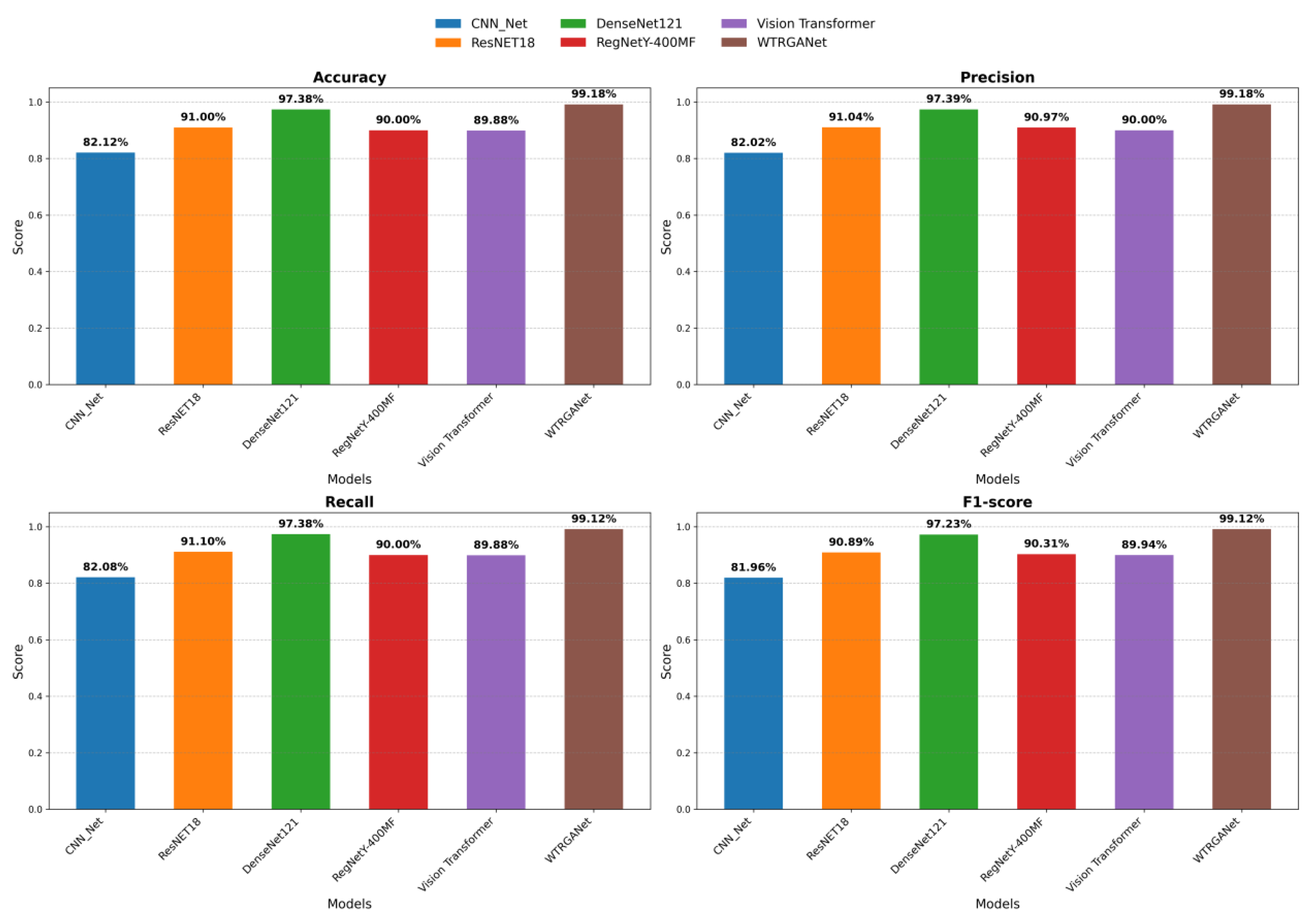
The comparative experimental results are shown in Table 4 From the results, WTRGANet demonstrates consistent and significant advantages in evaluation metrics such as accuracy, precision, recall, and F1-score. The design of WTRGANet, which combines wavelet transform with residual gated attention mechanisms, enables it to effectively extract multi-scale features while enhancing the model’s focus on key regions and channels. In the experiments, WTRGANet achieved an impressive accuracy of 0.9918. In comparison, models such as DenseNet-121, ResNet-18, RegNetY-400MF, and Vision Transformer (VIT) have also performed well on Kaggle’s leaderboard. DenseNet-121 improves feature transfer efficiency through its densely connected structure, achieving an accuracy of 0.9738. ResNet-18 and RegNetY-400MF performed well with accuracies of 0.9100 and 0.9000, respectively. Overall, WTRGANet demonstrates stronger advantages in extracting multi-scale features and handling noisy and blurry MRI images.
Figure 10.
Comparative analysis of visualisation of experimental results for different models.
As shown in Figure 11, the accuracy and loss curves during the training process demonstrate that WTRGANet exhibits fast convergence and superior training stability, avoiding common overfitting issues. Both the training and test set loss curves show a smooth downward trend, indicating the model’s strong generalization capability.
As shown in Figure 12, through the analysis of the confusion matrix,this study observe that WTRGANet achieves high accuracy in predicting all categories, especially in classifying mild and very mild dementia, with almost no misclassification. This result indicates that WTRGANet not only effectively distinguishes different pathological stages of Alzheimer’s Disease but also robustly handles data imbalance issues. Although other baseline models, such as ResNet18 and DenseNet-121, also perform well on certain metrics, WTRGANet’s multi-resolution feature extraction capability and the dynamic adjustment ability of its residual gated attention module enable it to more effectively address the diversity and challenges in the data, further improving overall classification accuracy.
4.5. Ablation Study
In this section, we conducted ablation experiments to thoroughly investigate the contribution of each key component in WTRGANet to the overall performance. To comprehensively evaluate the architectural design of WTRGANet and the role of its individual modules, we designed three ablation configurations: removing the wavelet transform convolutional layer (Without_WTConv), removing the residual gated attention module (Without_RGA), and removing both the wavelet transform convolutional layer and the residual gated attention module (Without_RGA_WTConv). The purpose of these experiments is to validate the independent effects of each module and analyze their impact on the final classification performance. The specific results of the ablation experiments are shown in Table 5.
Figure 13.
Comparative analysis of the visualisation of the results of ablation experiments.
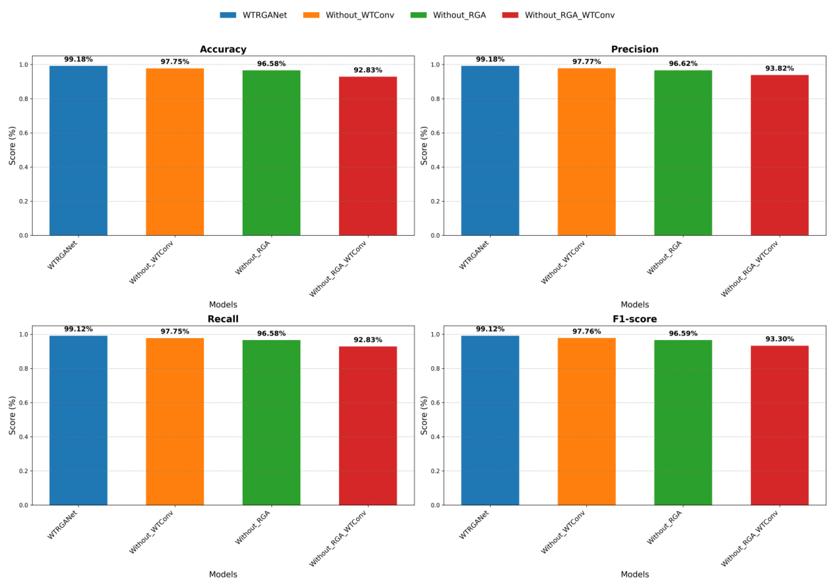
In the configuration without the wavelet transform convolutional layer (Without_WTConv), the performance of the WTRGANet model significantly declined. This indicates that the wavelet transform convolutional layer plays a crucial role in extracting multi-resolution features and expanding the receptive field. Without this module, the model loses the ability to extract detailed and structural information across different frequency domains, leading to an overall performance drop. In the configuration without the residual gated attention module (Without_RGA), the model’s performance also showed a noticeable decline. Although the precision, recall, and F1-score without the RGA module were 0.9662, 0.9658, and 0.9659, respectively, which is an improvement compared to the configuration without the wavelet transform convolutional layer, it still did not reach the level of the original model. Removing the RGA module means the model loses the ability to dynamically adjust feature map weights through channel and spatial attention mechanisms, directly impacting its ability to focus on key information when processing complex images. In the configuration without both the wavelet transform convolutional layer and the residual gated attention module (Without_RGA_WTConv), the model’s performance further declined, with precision, recall, and F1-score of 0.9382, 0.9283, and 0.9330, respectively. This result further validates the complementary roles of the wavelet transform convolutional layer and the RGA module in enhancing model performance. Without these two key modules, the model loses its ability to extract multi-resolution features and focus on key regions, resulting in a significant drop in classification accuracy. The results demonstrate that the high performance of WTRGANet stems from the effective integration of its modules, and the removal of any module has a significant negative impact on model performance.
5. Future Work
This study presents a novel deep learning model called WTRGANet, which achieves significant improvements in the task of classifying MRI images of Alzheimer’s disease by cleverly combining the wavelet transform and residual-gated attention mechanisms. The innovation of this work is that, for the first time, we systematically integrate the wavelet transform, a mathematical tool, into a deep convolutional neural network, enabling the model to simultaneously capture the feature representation of images at different scales.
Specifically, WTRGANet contains two key components:
First, the wavelet transform convolutional layer we designed breaks through the limitations of traditional convolutional operations by decomposing and reconstructing the image at multiple scales, which not only enlarges the sensory field of the network, but also particularly strengthens the ability to extract low-frequency features. Secondly, the residual gated attention module we developed creatively integrates the channel and spatial attention mechanisms, and achieves intelligent focusing and dynamic enhancement of key pathological features by introducing a gating strategy.
After rigorous experimental validation, WTRGANet demonstrates significant advantages in all evaluation metrics (statistical significance ). Detailed ablation analysis reveals two major sources of performance enhancement: multi-scale feature representation brings about performance gain, while the attention mechanism contributes about enhancement. Of particular note, the model performs particularly well in the most challenging task of early case recognition, reaching excellent levels of sensitivity and specificity of and , respectively.
The main contributions of this study can be summarised in three areas:
- (1)
- A novel multi-scale feature learning framework is established;
- (2)
- An efficient attentional feature enhancement scheme is proposed;
- (3)
- Providing reliable technical support for the early diagnosis of Alzheimer’s disease.
Looking forward to future research directions, we plan to extend the method in two dimensions: on the one hand, we will explore the applicability of the method in the diagnosis of other neurological disorders, such as brain tumour and Parkinson’s disease; on the other hand, we will investigate its performance in multi-task learning scenarios, including extended tasks, such as disease progression prediction and lesion pinpointing. These follow-up works will provide an important basis for our in-depth understanding of the generalisability and clinical application value of the method.
References
- Zvěřová, M. Clinical aspects of Alzheimer’s disease. Clinical biochemistry 2019, 72, 3–6. [Google Scholar] [CrossRef] [PubMed]
- Sloane, P.D.; Zimmerman, S.; Suchindran, C.; Reed, P.; Wang, L.; Boustani, M.; Sudha, S. The public health impact of Alzheimer’s disease, 2000–2050: potential implication of treatment advances. Annual review of public health 2002, 23, 213–231. [Google Scholar] [CrossRef] [PubMed]
- Pulido Chadid, A.M. Complex relationships between structural changes using brain Magnetic Resonance imaging in early diagnosis of Alzheimer’s Disease. PhD thesis, UNIVERSIDAD NACIONAL DE COLOMBIA, BOG, Colombia, 2014.
- Smits, M. MRI biomarkers in neuro-oncology. Nature Reviews Neurology 2021, 17, 486–500. [Google Scholar] [CrossRef] [PubMed]
- Ding, Y.; Sohn, J.H.; Kawczynski, M.G.; Trivedi, H.; Harnish, R.; Jenkins, N.W.; Lituiev, D.; Copeland, T.P.; Aboian, M.S.; Mari Aparici, C.; et al. A deep learning model to predict a diagnosis of Alzheimer disease by using 18F-FDG PET of the brain. Radiology 2019, 290, 456–464. [Google Scholar] [CrossRef] [PubMed]
- Raju, M.; Gopi, V.P.; Anitha, V.; Wahid, K.A. Multi-class diagnosis of Alzheimer’s disease using cascaded three dimensional-convolutional neural network. Physical and Engineering Sciences in Medicine 2020, 43, 1219–1228. [Google Scholar] [CrossRef] [PubMed]
- Ramírez, J.; Górriz, J.; Salas-Gonzalez, D.; Romero, A.; López, M.; Álvarez, I.; Gómez-Río, M. Computer-aided diagnosis of Alzheimer’s type dementia combining support vector machines and discriminant set of features. Information Sciences 2013, 237, 59–72. [Google Scholar] [CrossRef]
- Magnin, B.; Mesrob, L.; Kinkingnéhun, S.; Pélégrini-Issac, M.; Colliot, O.; Sarazin, M.; Dubois, B.; Lehéricy, S.; Benali, H. Support vector machine-based classification of Alzheimer’s disease from whole-brain anatomical MRI. Neuroradiology 2009, 51, 73–83. [Google Scholar] [CrossRef] [PubMed]
- Segovia, F.; Górriz, J.; Ramírez, J.; Salas-Gonzalez, D.; Álvarez, I.; López, M.; Chaves, R.; Initiative, A.D.N.; et al. A comparative study of feature extraction methods for the diagnosis of Alzheimer’s disease using the ADNI database. Neurocomputing 2012, 75, 64–71. [Google Scholar] [CrossRef]
- Ramírez, J.; Górriz, J.; Salas-Gonzalez, D.; Romero, A.; López, M.; Álvarez, I.; Gómez-Río, M. Computer-aided diagnosis of Alzheimer’s type dementia combining support vector machines and discriminant set of features. Information Sciences 2013, 237, 59–72. [Google Scholar] [CrossRef]
- Oliveira Jr, P.P.d.M.; Nitrini, R.; Busatto, G.; Buchpiguel, C.; Sato, J.R.; Amaro Jr, E. Use of SVM methods with surface-based cortical and volumetric subcortical measurements to detect Alzheimer’s disease. Journal of Alzheimer’s Disease 2010, 19, 1263–1272. [Google Scholar] [CrossRef] [PubMed]
- Hon, M.; Khan, N.M. Towards Alzheimer’s disease classification through transfer learning. In Proceedings of the 2017 IEEE International conference on bioinformatics and biomedicine (BIBM). IEEE; 2017; pp. 1166–1169. [Google Scholar]
- Liu, F.; Yuan, S.; Li, W.; Xu, Q.; Sheng, B. Patch-based deep multi-modal learning framework for Alzheimer’s disease diagnosis using multi-view neuroimaging. Biomedical Signal Processing and Control 2023, 80, 104400. [Google Scholar] [CrossRef]
- Venugopalan, J.; Tong, L.; Hassanzadeh, H.R.; Wang, M.D. Multimodal deep learning models for early detection of Alzheimer’s disease stage. Scientific reports 2021, 11, 3254. [Google Scholar] [CrossRef] [PubMed]
- Abrol, A.; Fu, Z.; Du, Y.; Calhoun, V.D. Multimodal data fusion of deep learning and dynamic functional connectivity features to predict Alzheimer’s disease progression. In Proceedings of the 2019 41st annual international conference of the IEEE engineering in medicine and biology society (EMBC). IEEE; 2019; pp. 4409–4413. [Google Scholar]
- Mallat, S. A wavelet tour of signal processing; Elsevier, 1999.
- Daubechies, I. Ten lectures on wavelets; SIAM, 1992.
Figure 1.
WTRGANet method processing flow block diagram.
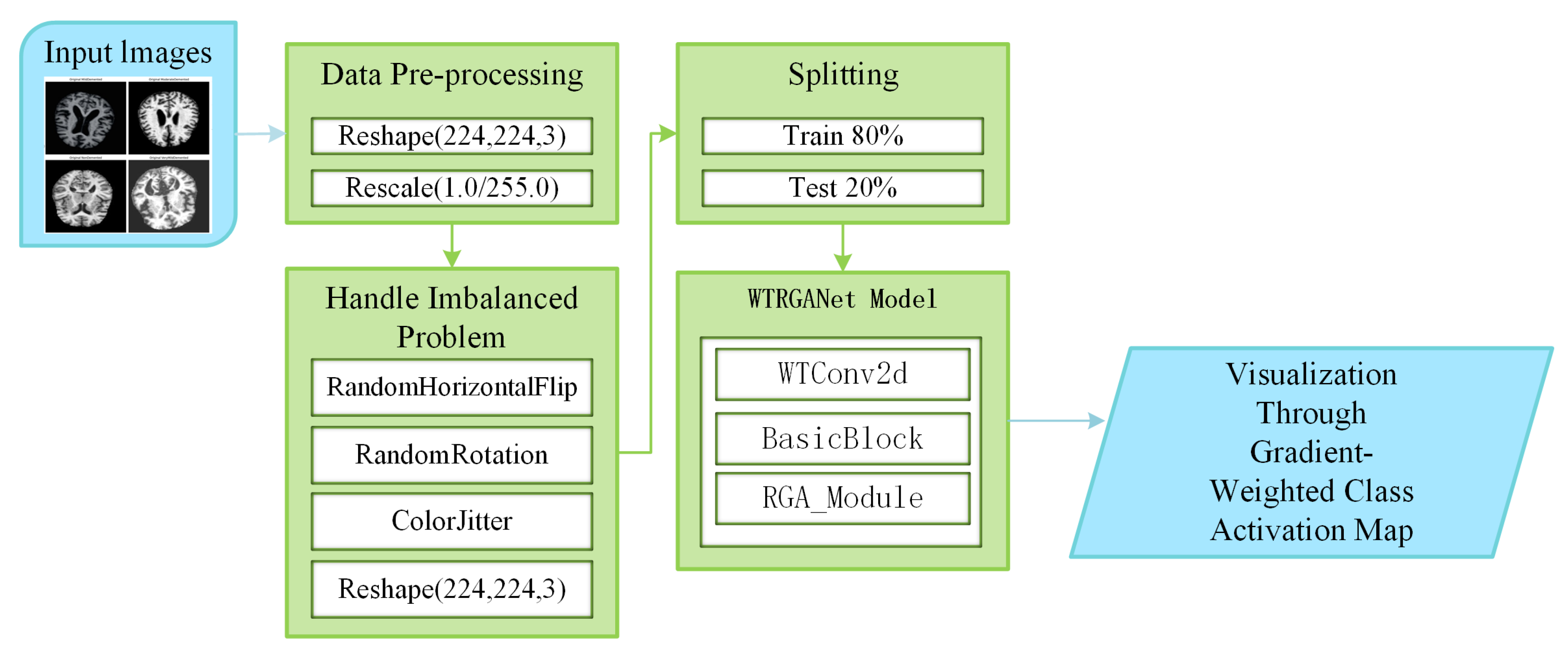
Figure 2.
WTRGANet overall network architecture diagram.
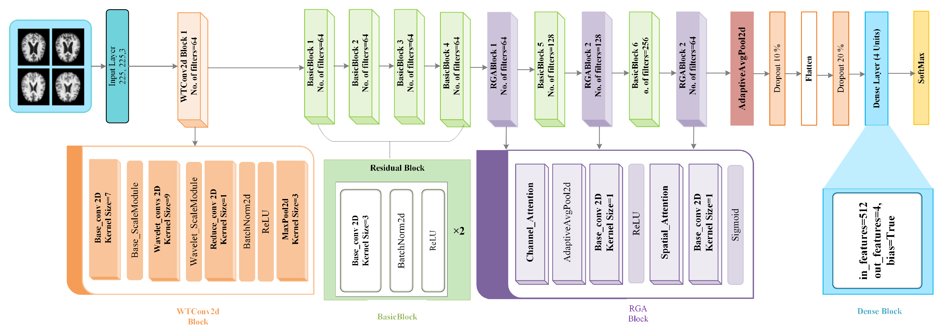
Figure 3.
Wavelet transform process diagram.
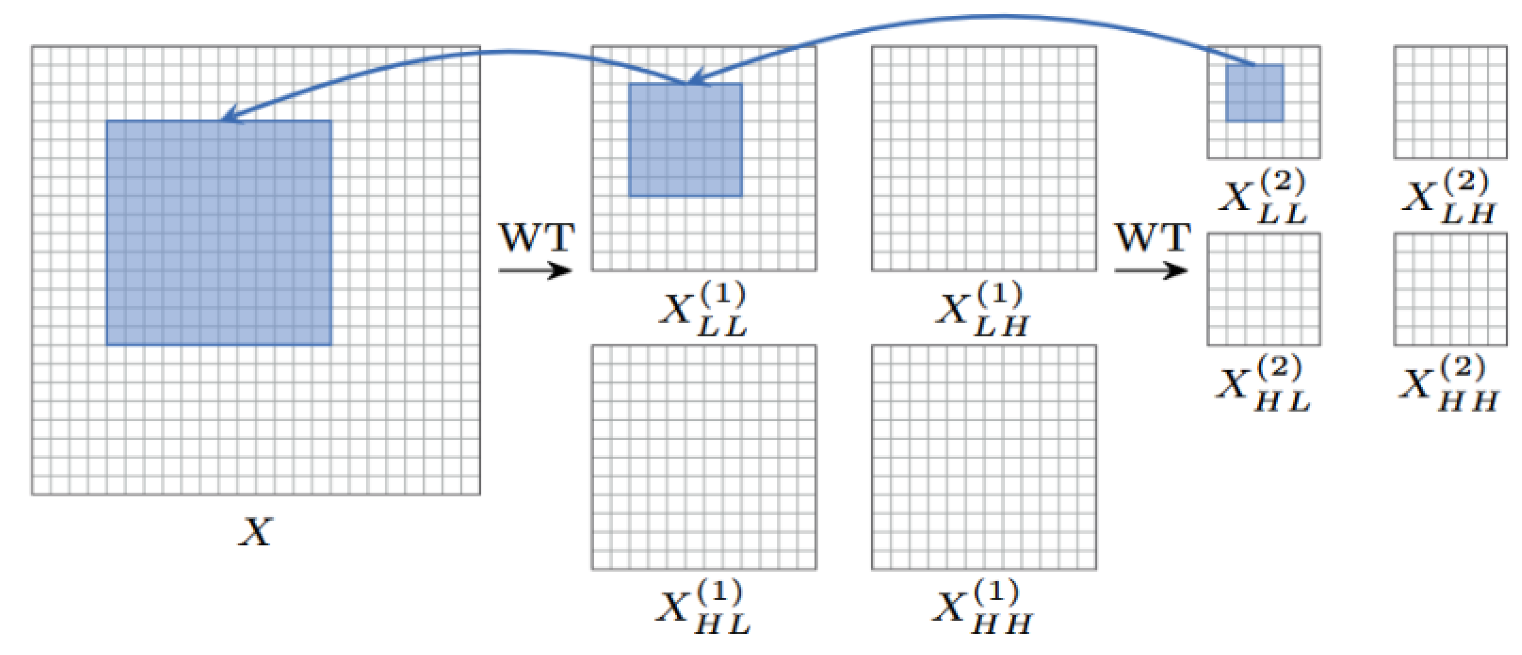
Figure 4.
Schematic of wavelet convolution processing of MRI images of Alzheimer’s disease.
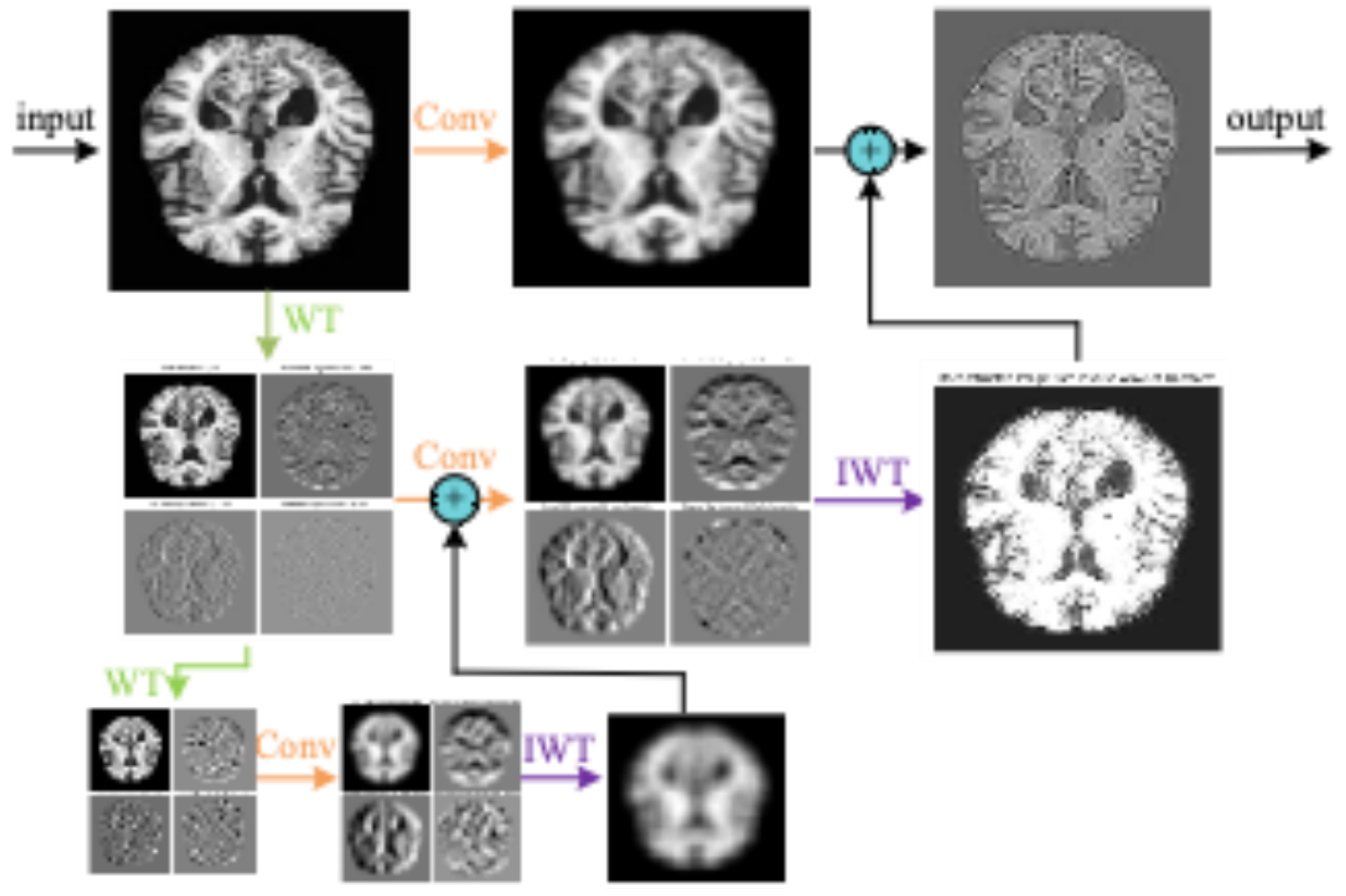
Figure 5.
Schematic representation of the attention mechanism processing of MRI image channels in Alzheimer’s disease.
Figure 5.
Schematic representation of the attention mechanism processing of MRI image channels in Alzheimer’s disease.
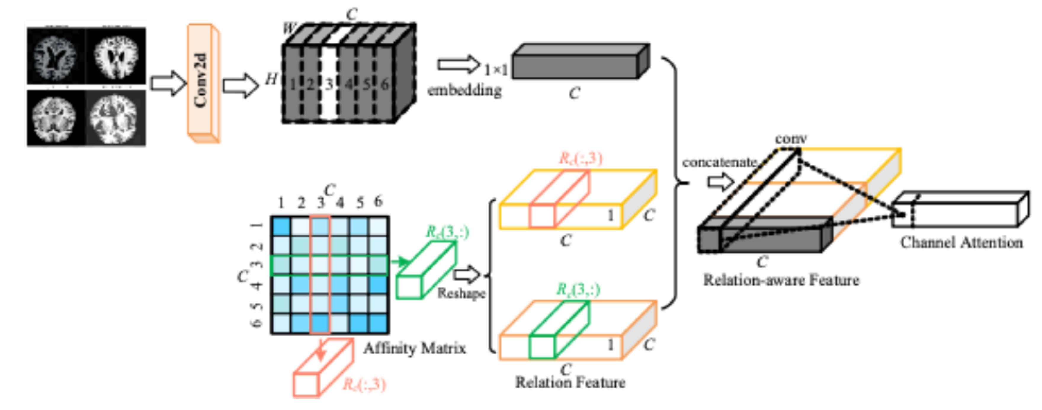
Figure 6.
Schematic diagram of spatial attention mechanism processing of MRI images of Alzheimer’s disease.
Figure 6.
Schematic diagram of spatial attention mechanism processing of MRI images of Alzheimer’s disease.
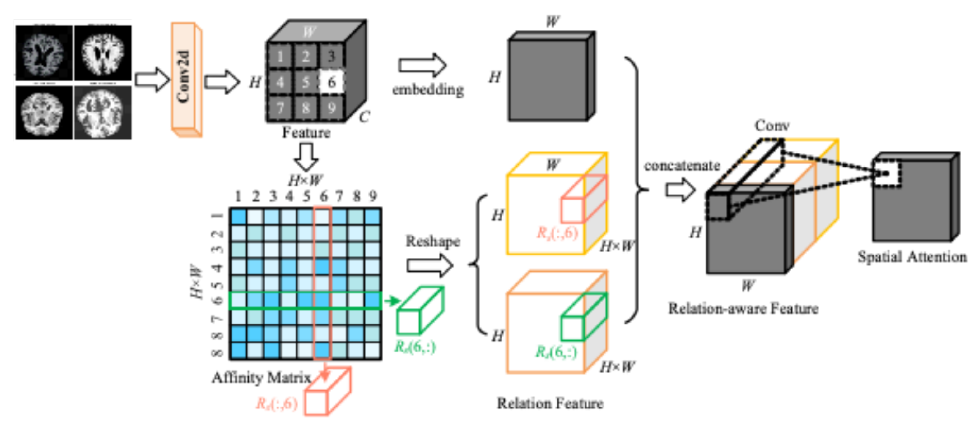
Figure 7.
Original image display on four categories.
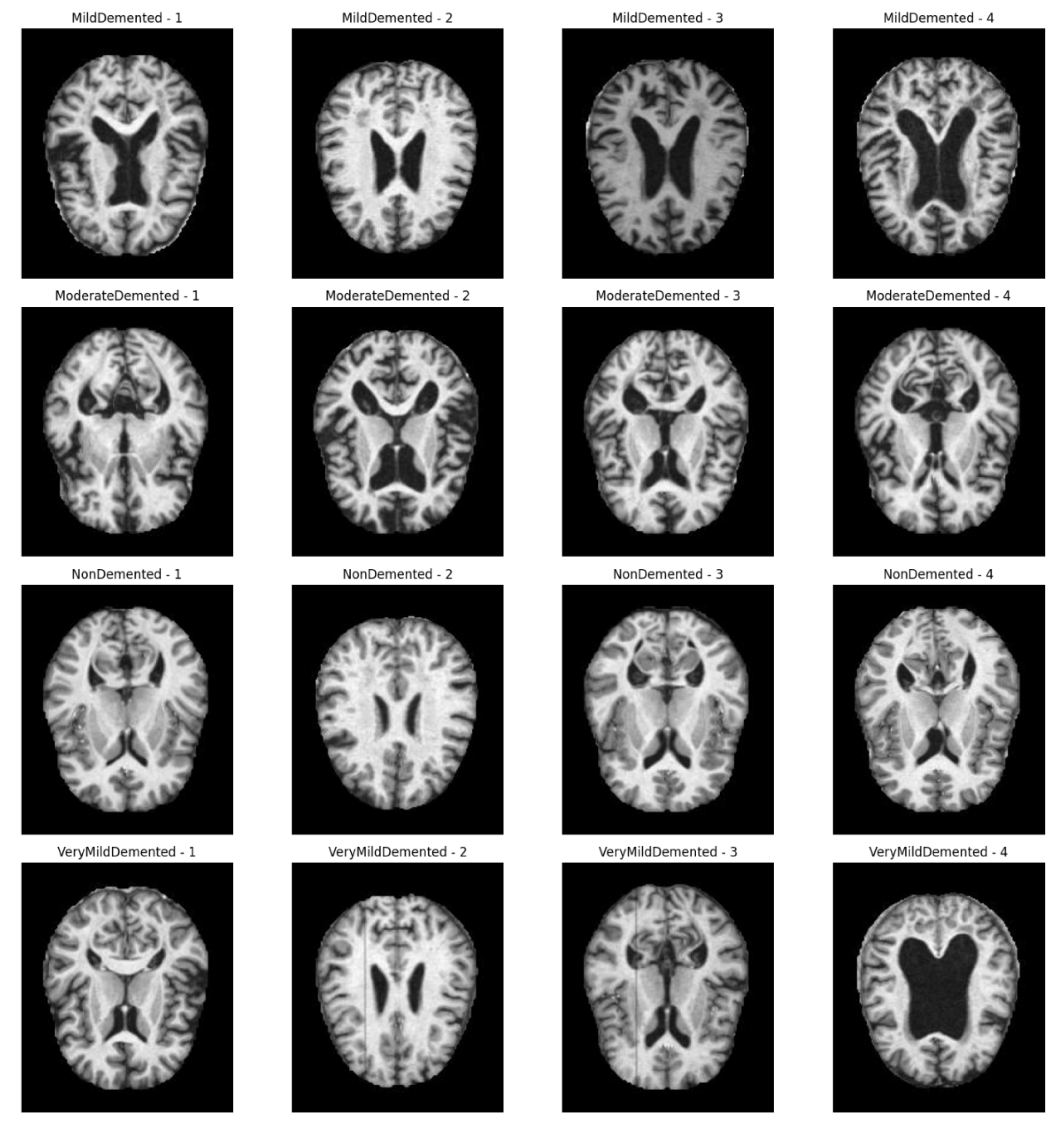
Figure 8.
Enhanced image display on four categories.
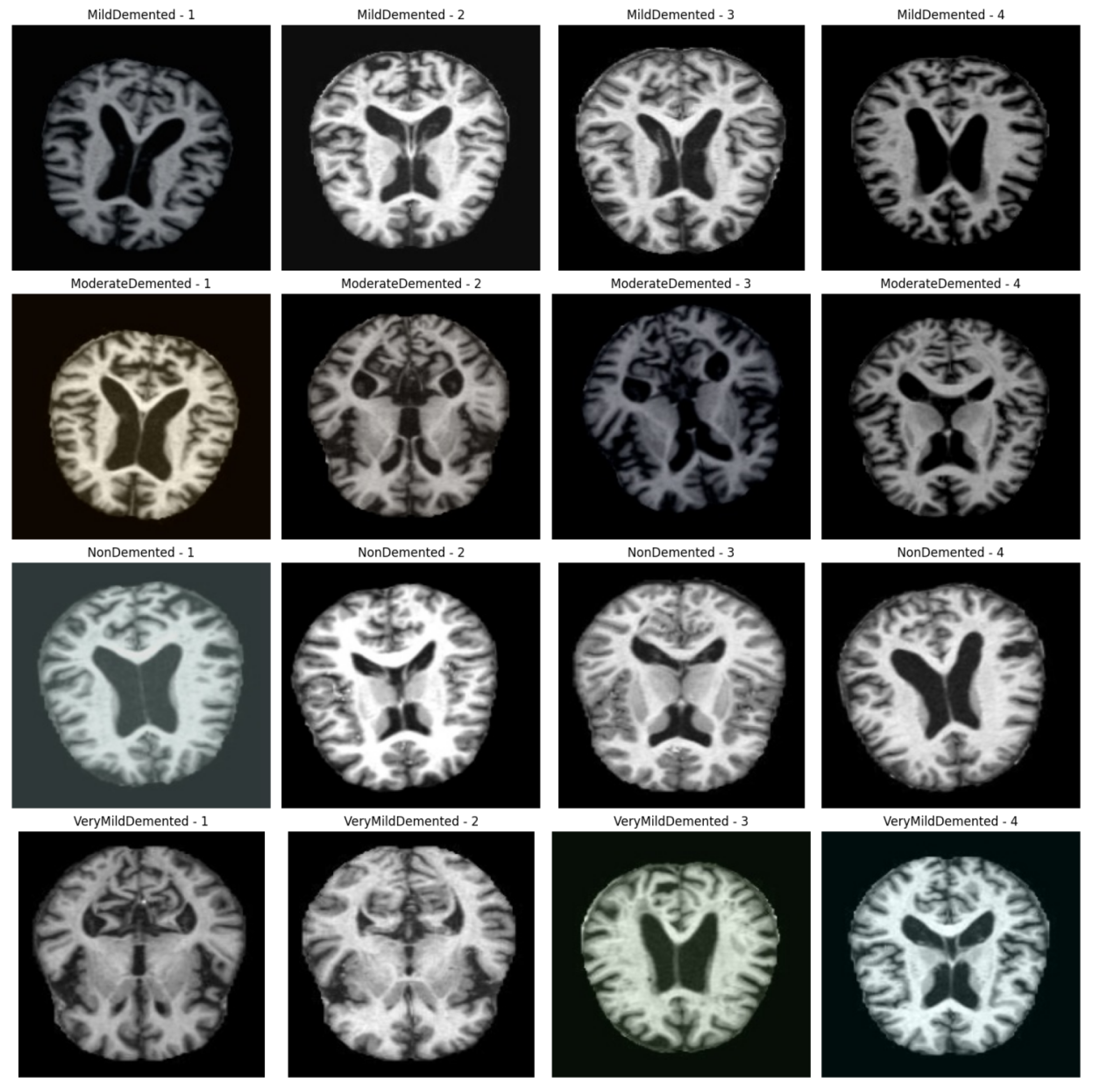
Figure 9.
Training and evaluation process for different models.
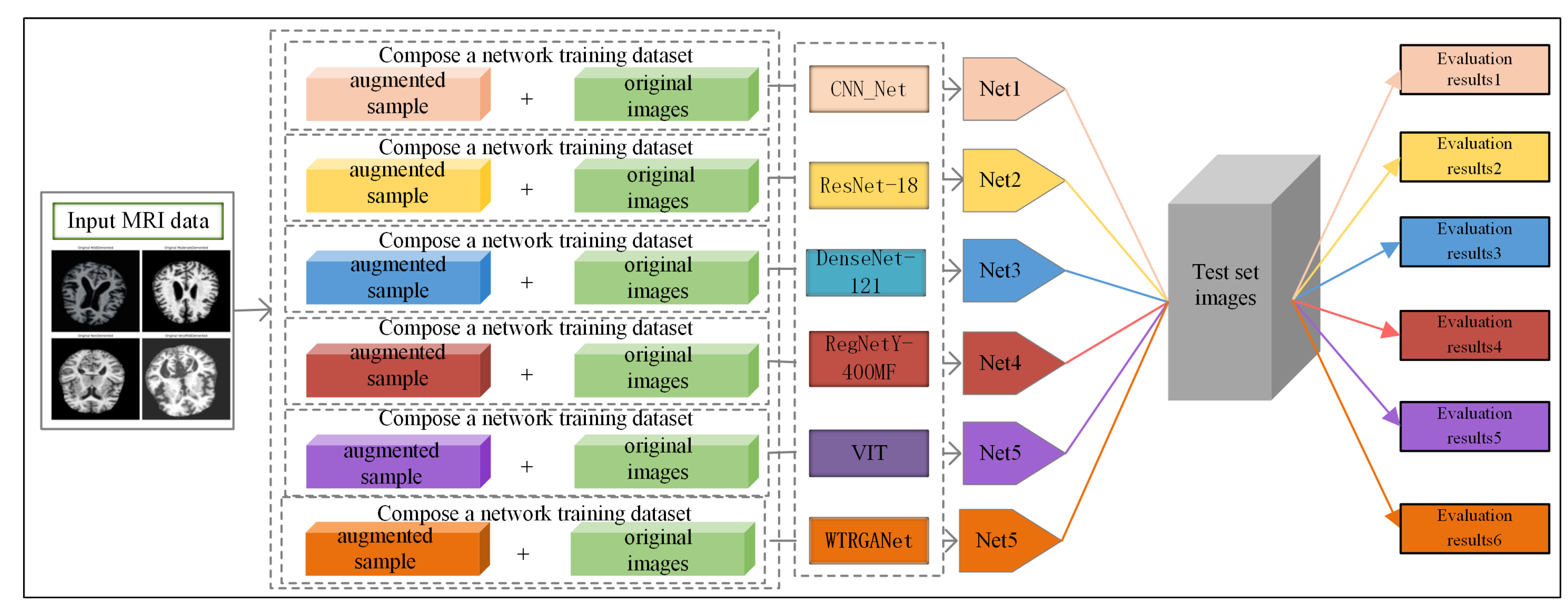
Figure 11.
Curves of accuracy and loss during model training.
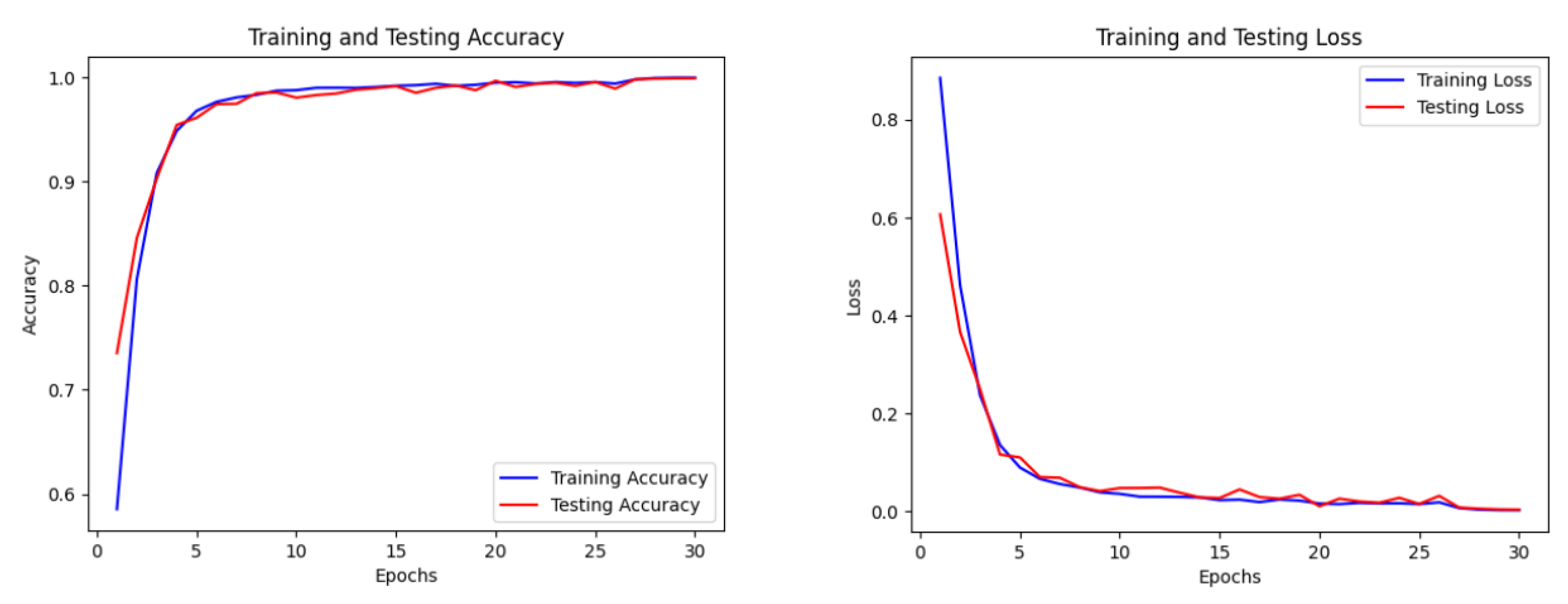
Figure 12.
Analysis of confusion matrices.
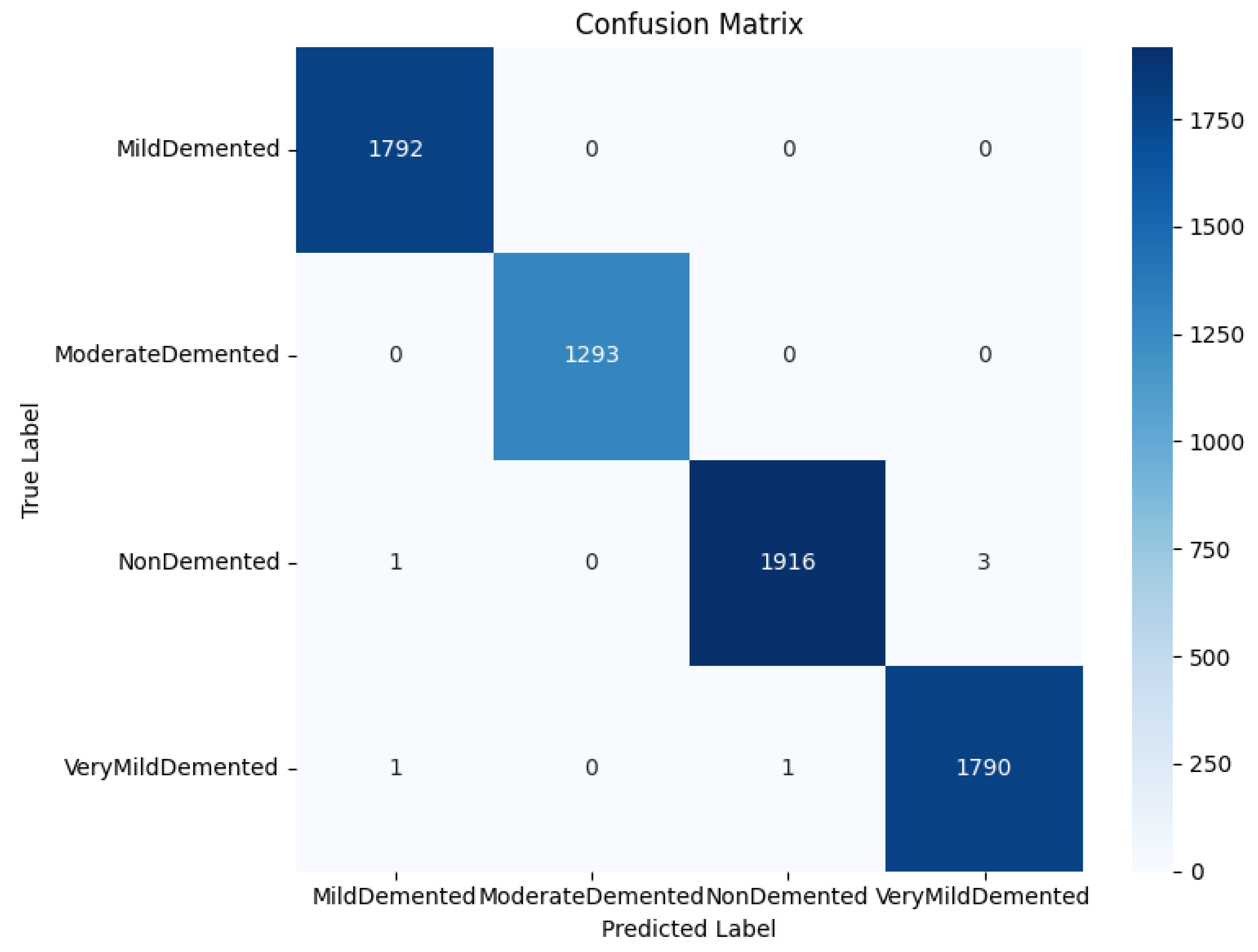
Table 2.
Data set division table.
| categories | Number of images after data enhancement |
Number of training sets |
Number of test sets |
|---|---|---|---|
| MildDemented | 8,960 | 7,168 | 1,792 |
| ModerateDemented | 6,464 | 5,171 | 1,293 |
| NonDemented | 9,600 | 7,680 | 1,920 |
| VeryMildDemented | 8,960 | 7,168 | 1,792 |
| total |
Table 3.
Optimal parameters for the WTRGANet model experiment.
| Sr:# | Parameter Name | Parameter Type |
|---|---|---|
| 1 | Optimizer | SGD |
| 2 | Learning rate | 0.01 |
| 3 | Batch size | 64 |
| 4 | Epochs | 20 |
| 5 | Call back | ReduceLROnPlateau |
| 6 | Hidden layer activation | ReLU |
| 7 | Output layer activation | SoftMAX |
| 8 | Loss function | CrossEntropyLoss |
| 9 | Optimizer type | Adam |
| 10 | Weight decay | 1e-4 |
| 11 | Data Normalization | Mean: , Std: |
Table 4.
Model Comparison Experimental Results.
| Model | Accuracy | Precision | Recall | F1-Score |
|---|---|---|---|---|
| CNN_Net | 0.8212 | 0.8202 | 0.8208 | 0.8196 |
| ResNet-18 | 0.9100 | 0.9104 | 0.9110 | 0.9087 |
| DenseNet-121 | 0.9738 | 0.9739 | 0.9738 | 0.9723 |
| RegNetY-400MF | 0.9000 | 0.9097 | 0.9000 | 0.9031 |
| Vision Transformer | 0.8988 | 0.9000 | 0.8988 | 0.8994 |
| WTRGANet(ours) |
Table 5.
Results of ablation experiments.
| Ablation | Accuracy | Precision | Recall | F1 |
|---|---|---|---|---|
| Without_WTConv | 0.9775 | 0.9777 | 0.9775 | 0.9776 |
| Without_RGA | 0.9658 | 0.9662 | 0.9658 | 0.9659 |
| Without_RGA_WTConv | 0.9283 | 0.9382 | 0.9283 | 0.9330 |
| WTRGANet(ours) |
Disclaimer/Publisher’s Note: The statements, opinions and data contained in all publications are solely those of the individual author(s) and contributor(s) and not of MDPI and/or the editor(s). MDPI and/or the editor(s) disclaim responsibility for any injury to people or property resulting from any ideas, methods, instructions or products referred to in the content. |
© 2025 by the authors. Licensee MDPI, Basel, Switzerland. This article is an open access article distributed under the terms and conditions of the Creative Commons Attribution (CC BY) license (http://creativecommons.org/licenses/by/4.0/).
Copyright: This open access article is published under a Creative Commons CC BY 4.0 license, which permit the free download, distribution, and reuse, provided that the author and preprint are cited in any reuse.


