Submitted:
25 April 2025
Posted:
27 April 2025
You are already at the latest version
Abstract
Alzheimer’s disease (AD) is a slow-growing neurological disorder that destroys human thought and consciousness. This disease directly affects the development of mental ability and neurocognitive function. The number of Alzheimer’s patients is increasing day by day, especially in the elderly over 60 years of age, and it gradually becomes a cause of their death. Machine learning (ML) and deep learning (DL) approaches have been developed in the literature to improve the diagnosis and classification of AD. Machine learning approaches have cumbersome feature selection. Deep learning has been used in recent research because it automatically selects features. This research aims to present a Swin Transformer wavelet for Alzheimer’s classification based on FMRI images in two-class, three-class and four-class modes. The proposed approach uses wavelet fusion in the Swin Transformer network to extract features. The outputs of the modified capsule are fed into a wavelet as feature vectors. The wavelet is a relevant feature selector in the proposed model. The Gray Wolf Optimization (GWO) method was used to find the model’s hyperparameters. The proposed approach achieved an accuracy of 0.9812 in 4-class classification, 0.9980 in 3-class classification, and 1.0 in 2-class classification. In the studies conducted in this research, the Swin Transformer wavelet+GWO model is the heaviest model in terms of the evaluation criteria Parameters(10e6), GFlops, and Memory (GB). This is while the EfficientNet model is the lightest in these criteria.
Keywords:
Alzheimer’s disease (AD)
; swin transformer
; wavelet
; gray wolf optimization (GWO)
; modified capsule
1. Introduction
According to the World Health Organization, more than 286 million people worldwide suffer from brain disease [1]. According to reports [2], 246 million people are mentally ill, and 39 million are in critical condition. As one of the largest and most complex parts of the body, the brain plays an important role in numerous functions, such as generating ideas, problem-solving, reasoning, decision-making, imagination and memory [1]. Alzheimer’s disease (AD), which affects millions of people, is the most common type of dementia. As people age, their anxiety about developing Alzheimer’s increases. Alzheimer’s disease slowly destroys brain cells and leaves patients unable to recognize family members. As a result, they become confused and lose the ability to recognize their surroundings. In advanced stages, they also lose the ability to eat, cough, and breathe [3].
The number of Alzheimer’s patients is expected to increase exponentially by 2050, with 152 million new cases of AD and dementia being diagnosed annually, or one every three seconds. AD symptoms, such as memory impairment, language and communication difficulties, and behavioral and psychological symptoms, overlap with vascular dementia (VD), making the diagnosis of AD challenging[4] [5]. Early and accurate diagnosis of AD is crucial for patient care, treatment, and prevention by monitoring its progression. Brain tumors are another severe condition that can be life-threatening to the brain. Since the blood vessels and nerves of the brain are at risk, tumors often develop there. Depending on the stage and malignancy of the tumor, it can cause partial or complete blindness [6]. Family history, ethnicity, and severe myopia are other contributing factors [7]. As a result, today’s most advanced societies increasingly need to discover rapid and automated early detection techniques. Medical imaging has also become a powerful tool for understanding brain activity. Magnetic resonance imaging (MRI) is a type of brain imaging that allows visualization of the structure and function of the brain. Medical professionals evaluate patients for signs and symptoms of AD and brain tumors. MRI can identify brain abnormalities associated with mild cognitive impairment (MCI) and predict which MCI patients will develop AD and brain tumors. MRI images are examined for abnormalities, such as reductions in the size of various brain regions that primarily affect memory[8].
Functional magnetic resonance imaging (fMRI) is yet another addition to the existing brain imaging techniques and methods for AD classification. It measures brain function by imaging blood flow alterations over time. This mechanism works based on blood flow’s coupling to neuronal activity. When a particular brain area is engaged, the blood flow to this specific area is also increased. Added to these imaging methods, resting-state functional MRI (rs-fMRI) has found several applications in research and has proven very high sensitivity for AD [9]. Using rs-fMRI, Greider et al. [10] found that reduced complexity of neural connectivity is directly associated with AD. Furthermore, rs-fMRI has been reported to reveal functional connectivity associated with cognitive impairments in elderly populations with health problems, MCI, and AD. Using traditional machine learning is challenging due to manual feature selection. Deep learning, as a multi-layered learning approach, attempts to learn using automatic feature selection. Deep learning has achieved remarkable results in medical applications [11,12,13], language models [14,15], and natural language processing[16,17]. In the field of neuroscience, various deep learning models have been employed to analyze fMRI data. Typically, analysis to distinguish between AD and CN states is performed using CNN models [18,19,20]. However, fMRI data have been used for binary classification in most studies. Further research needs to be done on multi-class classification of fMRI data.
In [21], the authors examined a case study of traditional machine learning approaches to predict Alzheimer’s Disease. Four standard machine learning models, including SVM, Logistic Regression, Decision Tree, and Random Forest, were used for the classification. The OASIS dataset was also used to evaluate these approaches. SVM obtained the best result in this study, and Logistic Regression obtained the worst result. SVM on OASIS data was able to achieve accuracy=0.92. The use of different features in classification is one of the advantages of this study, and the lack of comparison with deep learning approaches is one of its disadvantages. In [22], using SVM as a classification technique and improving feature selection in diagnosing AD is presented as a structured traditional ML approach. The accuracy of the method is reported to be 92.48%. The sensitivity and specificity were reported to be 86.92% and 90.76%, respectively.
The authors in [23] presented a method for diagnosing Alzheimer’s disease using image processing techniques and genetic algorithms for classification and prediction. The present study involves transforming Alzheimer’s disease into a cognitive disorder that serves as the initial feature of the input MRI images. This research used a genetic algorithm to predict and diagnose Alzheimer’s disease, and a support vector machine was used as a classification technique. The method reported a precision of 93.01%, a recall rate of 89.13%, and a feature recognition rate of 96.80%. The present study focuses on methods that use the ADNI dataset as the initial input data. Also, [24] reviewed traditional machine learning approaches for AD Diagnosis. [25] compared the performance of the machine learning models for Alzheimer’s Disease Early Detection. Logistic Regression, Decision Tree, Support Vector Machine, K-nearest Neighbors, Random Forest, Naïve Bayes, and Linear Discriminant Analysis models were used for classification. Also, the Alzheimer’s Disease Neuroimaging Initiative (ADNI) and the Open Access Series of Imaging Studies (OASIS) brain datasets were considered to evaluate these approaches. The Logistic Regression approach achieved the highest accuracy in both datasets. Selecting the correct features to provide a classifier is one of the advantages of this research. [26,?,27] other examples of studies that used traditional machine learning to classify Alzheimer’s.
[28] employed powerful deep learning models, such as VGG16, along with machine learning classifiers to thoroughly analyze MRI and PET scans for the detection of Alzheimer’s disease. Longer computation times accompanied the Support Vector Machine’s achievement of the highest accuracy (84%). Faster processing and strong predictive capabilities shown Random Forest’s potential. A hybrid deep learning approach for early detection was shown by several multimodal imaging studies using Convolutional Neural Networks along with LSTM algorithms. We explored several techniques to improve detection efficiency, including transfer learning, the selection of images based on entropy, as well as K-Means Clustering along with the Watershed method. Feature fusion importantly improved visual data representation, along with its analysis. RF’s robustness along with speed suits it for further Alzheimer’s research, despite SVM’s superior performance.
OViTAD [29] an optimized vision transformer. OViTAD uses AWS SageMaker infrastructure to predict healthy brains along with mild cognitive impairment MCI brains as well as Alzheimer’s disease AD brains using rs-fMRI and structural MRI data. OViTAD, through precise parameter optimization along with perceptive visualization of its attention mechanisms, importantly exceeded other deep learning models, as well as CNN-based ones, in multi-class classification; achieving outstandingly high average performances of 97% ± 0.0 and 99.55% ± 0.39 across three repetitions. [30] presented an effective segmentation approach (SAS) and a new classification model (HBOA-MLP) for Alzheimer’s disease early diagnosis based on fMRI images. It aimed at improving the accuracy of classification and shortening the computational time. Following preprocessing, SAS segmented the brain regions effectively, and feature vectors were extracted by Gabor and GLCM techniques. The vectors were optimized by the Honey Badger Optimization Algorithm (HBOA) and then used in a Multi-Layer Perceptron (MLP) model for classification. The HBOA-MLP model achieved a high accuracy of 99.44%; still, it faced a problem in dealing with large datasets due to the fully connected structure of the MLP network and its high number of parameters.
[31] proposes an automatic Alzheimer’s diagnosis system based on different frequency bands of rs-fMRI data and deep learning models. The system uses a high-order neuro-dynamic functional network taking slow4, slow5, and full-band ranges. Customized Alexnet and Inception blocks were utilized with SVM and KNN approaches for development. The presented deep ensemble networks demonstrated better performance without external feature selection. Slow5 features trained with customized networks attained better AD/MCI classifications. The results suggest that the characteristics of multiband rs-fMRI may serve as biomarkers for Alzheimer’s disease, facilitating a more efficient diagnostic framework.
Authors in [32] fused (sMRI) and (rs-fMRI) features to classify MCInc and AD from MCIc based on graph theory and machine learning. The model utilized cortical thickness, structural brain network, and sub-frequency functional brain network features. Feature selection techniques of RSFS, mRMR, and SS-LR were utilized, and SVM classifier and nested cross-validation were performed for classification. RSFS demonstrated the best accuracies in the classification between MCIc vs. MCInc and MCIc vs. AD. Combining several features enhanced classifying MCIc subjects from MCInc/AD. The framework that combined sMRI and fMRI data predicted MCI conversion, suggesting its potential to offer AD diagnostic markers [33] puts forward a new framework with rs-fMRI, PSI, and 2D-CNN for the abnormal brain functional connectivity detection in AD. This framework achieved the classification accuracy of 98.869% by fusing the brain topological and deep features. The framework using SVM classifier and 5-fold cross-validation classifies the AD and non-AD samples by extracting eight topological and deep features. The PSI network analysis reveals weaker connection strength and reduced small-world property in the brains of AD patients. The 2D-CNN model identifies deep features that represent abnormal connectivity patterns in AD patients, which contributes to understanding the pathogenesis of AD. This framework shows great potential for AD classification and elucidating the pathogenesis. [34] employs ResNet-18 architecture and rs-fMRI data to classify the stages of Alzheimer’s disease (AD). Three ResNet-18-based networks are trained and tested: 1CR, OTS, and FT. The FT network achieved the highest accuracy, which demonstrates the benefits of residual learning, pre-training, and transfer learning. The OTS network obtained the best average testing accuracy, which further proves the potential of deep learning approaches for AD classification.
Authors in [35] puts forward a deep learning framework for early Alzheimer’s disease detection with the use of resting-state fMRI data and clinical data. The framework involves specialized autoencoders in disentangling natural aging and disorder progression. It facilitates classification performance, reduces standard deviation over traditional classifiers, and avoids overfitting in a three-layer architecture for improved diagnostic accuracy by 25% over conventional approaches. This approach has the potential to merge brain network analysis with deep learning techniques for neurological disorder diagnosis in the earliest stages. [36] proposes a 3D-CNN-LSTM model for Alzheimer’s and other health diagnosis with 4D fMRI data. This model can extract spatial and temporal features effectively, with an accuracy of 96.4% using five-fold cross-validation. It outperforms the 3D-CNN model by utilizing both spatial and temporal information and has great potential to determine Alzheimer’s progression using analysis of 4D fMRI data.
The primary focus of this study is on the recent literature on automated classification and assessment of Alzheimer’s disease. We propose an integrated deep-learning architecture for Alzheimer’s disease classification with image data to achieve accurate and reliable classification in various clinical settings. The advanced techniques investigated have the potential to improve automated analysis and support clinical decision-making, thereby enabling early detection of the disease.
2. Methodology Overview
The proposed method for two-class and multi-class Alzheimer’s classification is shown in Figure 1. This method consists of three main parts: Swin Transformer, wavelet transform (WT), and Gray Wolf Optimization(GWO), and the details of each of these parts are discussed in more detail below.
The Swin Transformer (Shifted Window Transformer) is an innovative vision transformer model that addresses several computational challenges inherent in standard transformer models for image processing. Below is a breakdown of its methodology, focusing on key architectural details, attention mechanisms, and optimizations such as shifted window attention, along with an explanation of the associated formulas and figures.
2.1. Swin Transformer Overall Architecture
The Swin Transformer is designed to handle the computationally expensive operations typically associated with transformers, especially for high-resolution images. It is built on a hierarchical structure, similar to convolutional networks, but leverages transformer-based self-attention mechanisms to capture long-range dependencies between image patches.
-
Patch Splitting and Embedding: The first step in the model’s pipeline involves dividing an input image into small, non-overlapping patches (typically 4×4 pixels for this model). Each patch is treated as a token, and its feature is initialized using the concatenated RGB pixel values. The feature dimension of each patch is calculated as:The features are then passed through a linear embedding layer, which projects them to a higher-dimensional space (denoted as C, the number of channels).
- Transformer Blocks: The model consists of several modified Transformer blocks known as Swin Transformer blocks. These blocks are applied to the tokenized patches. The number of tokens, denoted as , remains constant in the early stages of the network. These blocks are referred to as Stage 1.
-
Hierarchical Representation: As the model deepens, a patch merging layer is introduced at each stage to reduce the number of tokens. This helps produce a more compact, hierarchical representation. For example, in Stage 2, the first patch merging layer concatenates features of neighboring patches and applies a linear transformation to reduce the token count by a factor of 4 (downsampling by a factor of 2 in both height and width).The model then proceeds through subsequent stages (Stages 3 and 4) with resolutions and , respectively.
- Hierarchical Structure: This approach is designed to be similar to conventional convolutional networks (like VGG and ResNet) in terms of resolution. The hierarchical design allows Swin Transformer to maintain high performance on vision tasks such as image classification and object detection, while also benefiting from the flexibility of transformers.
2.2. Shifted Window-Based Self-Attention
A key innovation in the Swin Transformer is the use of shifted window-based self-attention. Standard transformers compute global self-attention, where relationships between each token and all other tokens in the image are computed. This results in quadratic complexity, making it inefficient for tasks requiring high-resolution images or large numbers of tokens.
To address this, the Swin Transformer computes self-attention only within non-overlapping local windows. This significantly reduces computational complexity. For a given image with h×w patches, the self-attention complexity for global MSA and window-based MSA is expressed as:
The first formula represents the complexity of global self-attention, which scales quadratically with the number of patches hwhwhw. The second formula represents the complexity of window-based self-attention, which is linear with respect to the number of patches, provided the window size MMM is fixed.
Using window-based attention significantly reduces computational overhead, especially for large images, as it operates in linear time with respect to the number of patches.
A limitation of the window-based self-attention approach is that it doesn’t account for the relationships across neighboring windows. To overcome this, the Swin Transformer introduces a shifted window partitioning technique. In this approach, two consecutive Swin Transformer blocks alternate between regular window partitioning and shifted window partitioning, ensuring that cross-window dependencies are captured.
- In regular window partitioning, the image is split into windows of size (assuming ).
- In shifted window partitioning, the windows from the previous block are shifted by a certain offset, typically by half the window size.
The formulas for the computation in these blocks are as follows:
Here and represent the output features of the (SW-MSA) module and the MLP module for the block, respectively. The shifted window-based multi-head self-attention (SW-MSA) operates on shifted partitions, and the regular window-based attention (W-MSA) operates on the standard partitioning.
The shifted window partitioning method increases the number of windows when compared to regular partitioning, as some windows may be smaller than the standard size. A naive approach to handle this would involve padding smaller windows, but this leads to inefficient computations. The cyclic shift method solves this issue by shifting windows towards the top-left corner, keeping the number of windows consistent with the regular partitioning. This results in efficient batch processing without extra computational overhead.
To improve the self-attention mechanism, the model includes a relative position bias. This bias captures the positional relationships between tokens in each window, allowing the model to better understand spatial relationships. The relative position bias B is added to the self-attention computation:
Here Q, K, and V are the query, key, and value marrices, respectively and D is the query/key dimension, and B is the relative position bias mateix. The relative position bias is learned during training and helps the model capture the relative spatial relationships between image patches. This approach improves the performance of the model, particularly in tasks like image classification and object detection, as shown in experimental results.
Modified Capsule Network
The encoded features of the Swin Transformer are fed to the Capsule layer. The Capsule layer transforms the scalar features extracted by the Swin Transformer layer into vector-valued capsules to represent the features of the inputs. If the output of the Swin Transformer is and w is a weight matrix, then , which represents the prediction vector, is given by the following equations:
is the coupling coefficient, which is repeatedly adjusted by Dynamic Routing algorithm [37]. The length of the capsule determines the probability of the entity appearing. By changing the shape of all the initial capsules and screening the activation value of all the initial capsules, a certain proportion of the initial capsules with a higher activation value can be selected. This selection was introduced in [38] as CapsFilter. The general idea of this work is to use the median of the activation. Due to the significant difference in the activation value of the capsules, the average value of the activation value is minimal. In a group of data, the median is the value that represents the middle of all the data and has low sensitivity, meaning that it is not affected by the maximum or minimum value of the data distribution. Therefore, we sort the activation value of each capsule, take the median of the activation value as the basis for screening and divide it by the maximum activation value to ensure that it is a value proportional to (0, 1). The screening ratio increases when the activation value represented by the median is closer to the maximum activation value.
Here, the ’squash’ is a nonlinear mapping function by which the values produced by the vectors are converted into [0-1]. This function is carried out on as per the following formula:
2.3. Wavelet Transform (WT)
Wavelet transform (WT) was used in the Swin Transformer architecture to extract useful data. The WT consists of four components: one low-frequency and three high-frequency components. The low-frequency component, also called the low-low (LL) component, produces a sharper image of the input. The three high-frequency components (low-high (LH), high-low (HL), and high-high (HH)) ultimately produce sharper images. Previous studies and experiments have shown that the LL class of data is usually known as sharper and smoother images [?]. For more details on WT, see [?]. The WT is applied to the output of the capsule network. When the capsule generates hidden feature maps on the production of the Swin Transformer, the WT decomposes them into multiple subbands representing different frequency components. This decomposition enables the pre-conductor model to separate high-frequency components from low-frequency ones, increasing the model’s ability to recognize global and local patterns.
2.4. Gray Wolf Optimization(GWO)
GWO is used to optimize the model’s hyperparameters shown in Table 1. The goal of this optimization is to minimize the training and testing error. GWO is a metaheuristic optimization method that attempts to simulate the collective behavior of wolves in finding prey [39]. The behavior of gray wolves is inspiring for studying social behavior because these wolves behave respectfully towards each other in their social hierarchy. The social hierarchy of this species of wolves is determined based on the ability and strength of each individual, which leads to an effective hunting mechanism. Each wolf in the group can achieve a larger prey by cooperating and coordinating. In other words, cooperation between wolves is one of the main factors in gray wolves’ hunting success and survival. In these groups, an alpha wolf is chosen as the leader and has the highest social rank. In this social simulation, wolves are classified into four groups: Alpha, Beta, Delta and Omega, with different social behavior. The Alpha Wolf, as the leader, represents the best solution available. In a lower hierarchy, the Beta Wolf is the Alpha Wolf’s assistant and offers solutions similar to the Alpha Wolf. In a lower hierarchy than the Alpha Wolf is the Delta Wolf, an intermediary between the weaker wolves and the Beta. Finally, the Omega Wolves, the weakest of the group, act as the group’s protector against external attacks [39].
In this optimization method, at the beginning of the optimization, several wolves are randomly placed in the problem space and generate initial random solutions. The cost function calculates the proximity distance of each wolf to the prey, and the position of each wolf is updated according to this function. This update leads to the movement of Omega wolves towards Alpha, Beta and Delta wolves using a combination of distance and randomness of the parameters and . The following relations show the relationship between prey and predators mathematically[39]:
Where t represents the current number of iterations. represents the current locations of the prey and represents the current locations of the predator.
Where and , the coefficients are given by and , and represents the distance between the prey and the wolf. has a linear decrease with iterations, and and are randomly generated values in the interval . Hence, for the three wolves, , , and , that are traversing around the three leading wolves, , , and , equations 16 to 22 are valid [40].
The cost function is re-evaluated after these steps. In fact, the goal is that the wolf that finds a better solution than the others will move to higher ranks. This process is actually an optimization that continues as many times as the number of iterations or coverage of the problem. The best solution found is finally presented by Alpha Wolf as the final answer.
3. Material
3.1. Dataset
The Alzheimer’s disease dataset was collected from the open-source platform Kaggle. This dataset is available via the link1. This dataset contains 6400 MR images from four classes: Mild Demented (MID), Moderate Demented (MOD), Non-Demented (ND), and Very Mild Demented (VMD). The image size of this dataset is 176 × 208, which was resized to 176 × 176 for use in this study. Sample images of the four classes are shown in Figure 2.
Table 2 shows the distribution of the dataset with several images in the resulting dataset, which clearly states that the dataset has an unbalanced class. For this purpose, data augmentation was used, which took the help of 5 data augmentation techniques. Five images were created for each image. Table 3 shows the results of data augmentation on this data.
3.2. Deep Learning Library
In this research, Keras was used to implement neural networks. Keras2 is one of Python’s best open-source deep learning and neural network libraries. It can be run on top of TensorFlow or Theano. Keras is developed with a focus on rapid testing, allowing for easy and rapid prototyping of neural network models. In general, this framework is known as a high-level user interface. Table 4 shows the hardware and software specifications of this research.
4. Results
The results obtained by the proposed approach and the comparative approaches are given in Table 6. To evaluate the proposed model and comparative approaches, the following four evaluation criteria were used in classification task:
- Accuracy:
- Precision:
- Recall:
- F1-Score:
Four transfer approaches were used to compare the proposed approach. Transfer learning is an advanced technique in machine learning that allows a model trained on one task to be repurposed for a different yet related task. This approach capitalizes on the knowledge embedded in a pre-trained model, typically developed on a large-scale dataset, to improve the performance of a new model, especially when the available data for the new task is limited. The pre-trained model layers, which have already learned to recognize general features such as edges, textures, and shapes, provide a solid foundation that can be fine-tuned to identify more specific patterns relevant to the new task. In doing so, transfer learning reduces the time required for training and increases the model’s effectiveness, making it a valuable tool in scenarios where data is scarce. In the context of medical image analysis, transfer learning is particularly beneficial[41]. Medical imaging tasks often involve complex patterns and subtle changes that are challenging to identify, especially with limited annotation data. By using models pre-trained on large datasets, transfer learning enables the application of these models to medical images, which can be tuned to focus on specific disease features. This improves the accuracy and robustness of the model and ensures that high-quality results can be achieved even with smaller datasets. As a result, transfer learning has become a critical component in developing advanced medical imaging solutions, contributing to diagnostic accuracy and computational efficiency advances. These approaches are as follows:
- EfficientNet: EfficientNet is a family of convolutional neural networks that optimizes accuracy and efficiency by increasing the model dimensions (depth, width, and resolution) in a balanced manner. This approach results in improved performance with much fewer parameters compared to traditional models, making it an excellent choice for high-accuracy tasks in medical image classification [42].
- Xception: A perception-based architecture that replaces perceptual modules with deep separable convolutions (deep convolutions followed by point convolutions). It does this by first obtaining correlations between features and then spatial correlations. This allows for more efficient use of model parameters[43].
- Inception: The Inception model, also known as GoogLeNet, is a deep convolutional neural network known for its distinctive architecture that combines multiple convolutional filters of different sizes in each layer. This innovative design allows the model to capture complex details and larger patterns simultaneously, resulting in highly efficient image processing. By employing 1x1 convolutions to reduce dimensionality before applying larger filters, Inception achieves high accuracy with fewer parameters and reduced computational complexity. When used in transfer learning, the pre-trained Inception model is a strong foundation, providing a robust base of multi-scale features that can be fine-tuned for specialized tasks such as medical image classification and localization. Its ability to efficiently process complex visual information makes it an ideal choice for applications that require precise image analysis, improving performance even with limited new data [44].
- DenseNet: DenseNet connects each layer to every other layer in a feedforward fashion, ensuring maximum information flow between layers. This densely connected architecture reduces the number of parameters while improving feature reuse, making DenseNet efficient and effective for the accurate analysis of medical images. DenseNet121 was used in this study. All of these models use ImageNet weights for training [45].
To test the models, 0.8 of the data was considered as training data and 0.20 of the data was considered as testing data. Also, the following 5 data augmentation techniques were used in the preprocessing process:
- Scaling(S):
- Rotation(R):
- Noise(N):
- Random translation(Rt):
- Gamma correction(Gc):
The data sets are split into two sets: training and testing . The specifications of the model and its hyper-parameters are summarized in Table 5, respectively.
The EfficientNetB3 approach was able to achieve Accuracy=0.9703, Precision=0.9711, Recall=0.9703, and F1=0.9706 on the 4-class classification (see Table 6). The Xception approach was able to achieve better results than EfficientNetB3 and achieved Accuracy=0.9727, Precision=0.9726, Recall=0.9719, and F1=0.9722. The worst result in the 4-class classification was achieved by the Inception V3 approach, which also achieved Accuracy=0.8953, Precision=0.8958, Recall=0.8938, and F1=0.8947. The approach achieved better results than InceptionV3 and worse than EfficientNetB3. This approach was able to achieve Accuracy=0.9578, Precision=0.9578, Recall=0.9570, and F1=0.9573. The two proposed Swin Transformer-based approaches were able to achieve results above 0.97. The results obtained show the highest competition among the four classes. The Swin Transformer wavelet approach was able to achieve Accuracy=0.9753, Precision=0.9751, Recall=0.9763, and F1=0.9756, and the Swin Transformer wavelet+ GWO approach was able to achieve Accuracy=0.9812, Precision=0.9812, Recall=0.9822, and F1=0.9816.

Table 6.
Four class classification on Alzheimer dataset. The bold represents the highest results/accuracy achieved for each experiment.
Table 6.
Four class classification on Alzheimer dataset. The bold represents the highest results/accuracy achieved for each experiment.
| Model | Accuracy | Precision | Recall | F1 |
|---|---|---|---|---|
| EfficientNetB3[42] | 0.9703 | 0.9711 | 0.9703 | 0.9706 |
| Xception[43] | 0.9727 | 0.9726 | 0.9719 | 0.9722 |
| InceptionV3[44] | 0.8953 | 0.8958 | 0.8938 | 0.8947 |
| DenseNet121[45] | 0.9578 | 0.9578 | 0.9570 | 0.9573 |
| Swin Transformer wavelet | 0.9753 | 0.9751 | 0.9763 | 0.9756 |
| Swin Transformer wavelet+ GWO | 0.9812 | 0.9812 | 0.9822 | 0.9816 |
The results of the three-class classification are given in Table 7. In the three-class classification on the Mild, Moderate, and Non-classes, the best result was obtained by the Swin Transformer wavelet+ GWO approach. The Swin Transformer wavelet approach also achieved an accuracy of 0.9970. Regarding the Mild, Moderate, and Very mild classifications, the best result was obtained using the Swin Transformer wavelet+ GWO approach. The two EfficientNetB3 and Swin Transformer wavelet approaches achieved almost equal results. The worst result on this classification was obtained by InceptionV3. In the three-class classification of Mild, Non, Very Mild, the Swin Transformer wavelet+ GWO approach achieved an accuracy of 0.9843. The worst result in the Mild, Non, Very Mild classification was obtained by the DenseNet121 approach. In the Moderate, Non, and Very Mild classifications, the best results were obtained by the Swin Transformer wavelet and Swin Transformer wavelet+ GWO approaches. The worst result was obtained by InceptionV3.
The results of a two-class classification in 6 different combinations of classes are given in Table 8. The Swin Transformer wavelet and Swin Transformer wavelet+ GWO models on Mild and Moderate were able to achieve an accuracy of 0.99. The two approaches, EfficientNetB3 and InceptionV3, achieved the weakest result in this classification. In Mild and Very Mild classification, the Swin Transformer wavelet+ GWO approach was able to achieve an accuracy of 0.9907, which is the highest accuracy in the tested models. The two models, EfficientNetB3 and InceptionV3, achieved an accuracy of 0.9204, which is the worst result in the tested models. The three approaches, DenseNet121, Swin Transformer wavelet, and Swin Transformer wavelet+ GWO, were able to achieve an accuracy of 1 on the binary classification of Mild and Non-classes. The other models in this class achieved an accuracy of 0.96. In the two classes Moderate and Non, the Xception, DenseNet121, Swin Transformer wavelet, and Swin Transformer wavelet+ GWO models were able to achieve an accuracy of 1. The other models achieved a high accuracy of 0.99. In the Moderate and Very Mild binary classification, the three approaches EfficientNetB3. Swin Transformer wavelet and Swin Transformer wavelet+ GWO were able to achieve an accuracy of 1. The Non and Very Mild binary classification is relatively the most difficult classification in the tested models, and the proposed Swin Transformer wavelet+ GWO model was able to achieve an accuracy of 0.9798.
The results of 5-fold cross-validation in four-class classification are shown in Table 9. The EfficientNetB3, Xception, InceptionV3, and DenseNet121 models achieved the highest results in Fold5, Fold1, Fold2, and Fold4. Adding Wavelet in Swin Transformer improved the model and achieved a maximum accuracy of 0.9816, which was in Fold1. Adding GWO to the Swin Transformer wavelet also improved the model slightly. The model achieved a maximum accuracy of 0.9875 in Fold1. According to Table 10, adding a wavelet after the network improves the model performance, which can be seen with a small p-value (less than 0.05). However, adding GWO after the wavelet does not have much effect on the model accuracy because the p-values are very significant, indicating that the statistical difference is small if optimization is used after the wavelet transform.
The bar plot of different approaches in 2, 3, and 4-class classification is shown in Figure 3. Figure 3-a shows the comparison of the models’ performance in two-class Alzheimer’s classification. Also shown in Figure 3-b and Figure 3-c are three and four-class classifications. According to the bar graphs, the proposed approach has the highest efficiency among the evaluated approaches.
In the following, Figure 4, Figure 5, Figure 6, Figure 7, Figure 8, Figure 9, Figure 10, Figure 11, Figure 12, Figure 13 and Figure 14 show the confusion matrix results for different approaches and different classifications.
4.1. Result on OASIS
To assess the comprehensiveness of the model, the OASIS dataset was also evaluated. The frequency of classes in this dataset is shown in Figure 15. The frequency of the number of patients in each category is also shown in Figure 16.
In the OASIS dataset, all models recorded very high performance. Table 11 shows the results obtained in this dataset. The EfficientNetB3 model achieved Accuracy=0.9898 and F1=0.9897 on this dataset. The Exception and InceptionV3 models recorded close accuracy, achieving an accuracy of 0.9983 and 0.9981, respectively. The DenseNet121 model had the highest model performance among the tested baseline methods. It achieved an accuracy of 0.9991 and F1 of 0.9999. The proposed models based on Swin Transformer achieved an accuracy of 1.0 on this dataset. These models also achieved an accuracy of 1.0 in the non-use mode and using GWO in other evaluation criteria.
4.2. Models Complexity
In this context, three indicators were used for evaluating the complexity of the models studied: Parameters(10e6) the number of learnable and unlearnable parameters of the model, GFlops showing floating-point operations (additions, subtractions, multiplications, and divisions), and Memory (in GB) the amount of RAM used in training the model on the data (see Table 12). The EfficientNet model has the lowest Parameters(10e6), GFlops, and Memory (GB) among the tested models. The Xception model is the second least parameterized model with 105.1 parameters. In terms of GFlops, this model is more than DenseNet121. Also, IncetionV3 has Parameters(10e6)= 144.1, GFlops=501.22, and Memory (GB)= 5.39, which is a costly model compared to the EfficientNet, Xception, and DenseNet121 models. Swin models are computationally and memory-intensive. This model, combined with GWO, can occupy a maximum of 8.2 GB of RAM.
5. Conclusion
Our study evaluated the performance of EfficientNetB3, Xception, InceptionV3, Swin Transformer wavelet, and Swin Transformer wavelet+ GWO algorithms in Alzheimer’s disease classification. These models basically use transfer learning and initial weights from ImageNet. In this study, classification was investigated in terms of two, three, and four classes. Five data augmentation methods were applied in preprocessing on the data. The results showed that Swin Transformer wavelet+ GWO achieved the highest accuracy among the tested models. The combination of Swin Transformer and wavelet was effective in all three categories of classification. On the other hand, choosing GWO to optimize the parameters led to better results. This improvement in 2-class classification ended with an accuracy of 1. However, using GWO to find the optimal values is very time-consuming. Using approaches based on recurrent networks such as [46,47,48] can lead to better results in combination with Swin Transformer. Furthermore, expanding the dataset size and incorporating more diverse features could improve model generalization and performance across different groups. Overall, these research directions offer promising avenues for advancing the diagnosis and management of Alzheimer’s disease.
Author Contributions
All authors contribute the writing the manuscript, concepts, methodology, design of the proposed models, experimental results analysis, the software of the proposed models, dataset collection, resources, visualization, implementation of the models, similarity reduction, and the editing of the manuscript, the review of the writing and grammatical errors for the manuscript, validation of the results, and supervision of the proposed work.
Funding
No funding.
Institutional Review Board Statement
INot applicable.
Informed Consent Statement
Not applicable.
Data Availability Statement
The datasets used and analysed during the current study are available from the corresponding author on reasonable request.
Conflicts of Interest
The authors declare no competing interests.
References
- Anton, A.; Fallon, M.; Cots, F.; Sebastian, M.A.; Morilla-Grasa, A.; Mojal, S.; Castells, X. Cost and detection rate of glaucoma screening with imaging devices in a primary care center. Clinical Ophthalmology 2017, pp. 337–346.
- Ibrahim, R.; Ghnemat, R.; Abu Al-Haija, Q. Improving Alzheimer’s disease and brain tumor detection using deep learning with particle swarm optimization. AI 2023, 4, 551–573. [Google Scholar] [CrossRef]
- Ibrahim, R.; Ghnemat, R.; Abu, A.H. Q. Improving Alzheimer’s Disease and Brain Tumor Detection Using Deep Learning with Particle Swarm Optimization. AI 2023, 4, 551–573, 2023. [Google Scholar] [CrossRef]
- Castellazzi, G.; Cuzzoni, M.G.; Cotta Ramusino, M.; Martinelli, D.; Denaro, F.; Ricciardi, A.; Vitali, P.; Anzalone, N.; Bernini, S.; Palesi, F.; et al. A machine learning approach for the differential diagnosis of Alzheimer and vascular dementia fed by MRI selected features. Frontiers in neuroinformatics 2020, 14, 25. [Google Scholar]
- Huang, J.; van Zijl, P.C.; Han, X.; Dong, C.M.; Cheng, G.W.; Tse, K.H.; Knutsson, L.; Chen, L.; Lai, J.H.; Wu, E.X.; et al. Altered d-glucose in brain parenchyma and cerebrospinal fluid of early Alzheimer’s disease detected by dynamic glucose-enhanced MRI. Science advances 2020, 6, eaba3884. [Google Scholar]
- Zaw, H.T.; Maneerat, N.; Win, K.Y. Brain tumor detection based on Naïve Bayes Classification. In Proceedings of the 2019 5th International Conference on engineering, applied sciences and technology (ICEAST). IEEE, 2019, pp. 1–4.
- Ghnemat, R.; Khalil, A.; Abu Al-Haija, Q. Ischemic stroke lesion segmentation using mutation model and generative adversarial network. Electronics 2023, 12, 590. [Google Scholar] [CrossRef]
- Korolev, S.; Safiullin, A.; Belyaev, M.; Dodonova, Y. Residual and plain convolutional neural networks for 3D brain MRI classification. In Proceedings of the 2017 IEEE 14th international symposium on biomedical imaging (ISBI 2017). IEEE, 2017, pp. 835–838.
- Gauthier, S.; Reisberg, B.; Zaudig, M.; Petersen, R.C.; Ritchie, K.; Broich, K.; Belleville, S.; Brodaty, H.; Bennett, D.; Chertkow, H.; et al. Mild cognitive impairment. The lancet 2006, 367, 1262–1270. [Google Scholar]
- Grieder, M.; Wang, D.J.; Dierks, T.; Wahlund, L.O.; Jann, K. Default mode network complexity and cognitive decline in mild Alzheimer’s disease. Frontiers in neuroscience 2018, 12, 770. [Google Scholar]
- Ahmadi, M.; Nia, M.F.; Asgarian, S.; Danesh, K.; Irankhah, E.; Lonbar, A.G.; Sharifi, A. Comparative analysis of segment anything model and u-net for breast tumor detection in ultrasound and mammography images. arXiv preprint arXiv:2306.12510 2023.
- Wang, J.; Wang, S.; Zhang, Y. Deep learning on medical image analysis. CAAI Transactions on Intelligence Technology 2025, 10, 1–35. [Google Scholar]
- Javed, H.; El-Sappagh, S.; Abuhmed, T. Robustness in deep learning models for medical diagnostics: security and adversarial challenges towards robust AI applications. Artificial Intelligence Review 2025, 58, 1–107. [Google Scholar]
- Farhadi Nia, M.; Ahmadi, M.; Irankhah, E. Transforming dental diagnostics with artificial intelligence: advanced integration of ChatGPT and large language models for patient care. Frontiers in Dental Medicine 2025, 5, 1456208. [Google Scholar]
- Shool, S.; Adimi, S.; Saboori Amleshi, R.; Bitaraf, E.; Golpira, R.; Tara, M. A systematic review of large language model (LLM) evaluations in clinical medicine. BMC Medical Informatics and Decision Making 2025, 25, 117. [Google Scholar]
- Nargesi, A.A.; Adejumo, P.; Dhingra, L.S.; Rosand, B.; Hengartner, A.; Coppi, A.; Benigeri, S.; Sen, S.; Ahmad, T.; Nadkarni, G.N.; et al. Automated identification of heart failure with reduced ejection fraction using deep learning-based natural language processing. Heart Failure 2025, 13, 75–87. [Google Scholar] [PubMed]
- Barde, A.; Kaimal, V.; Barde, S.; Sharma, S. Detection and Prevention of Fake News and Hate Speech through Machine Learning and Natural Language Processing. In Text and Social Media Analytics for Fake News and Hate Speech Detection; Chapman and Hall/CRC, 2025; pp. 262–279.
- Eskildsen, S.F.; Coupé, P.; García-Lorenzo, D.; Fonov, V.; Pruessner, J.C.; Collins, D.L.; Initiative, A.D.N.; et al. Prediction of Alzheimer’s disease in subjects with mild cognitive impairment from the ADNI cohort using patterns of cortical thinning. Neuroimage 2013, 65, 511–521. [Google Scholar] [PubMed]
- Vemuri, P.; Jones, D.T.; Jack, C.R. Resting state functional MRI in Alzheimer’s Disease. Alzheimer’s research & therapy 2012, 4, 1–9. [Google Scholar]
- Khazaee, A.; Ebrahimzadeh, A.; Babajani-Feremi, A.; Initiative, A.D.N.; et al. Classification of patients with MCI and AD from healthy controls using directed graph measures of resting-state fMRI. Behavioural brain research 2017, 322, 339–350. [Google Scholar]
- Bari Antor, M.; Jamil, A.S.; Mamtaz, M.; Monirujjaman Khan, M.; Aljahdali, S.; Kaur, M.; Singh, P.; Masud, M. A comparative analysis of machine learning algorithms to predict alzheimer’s disease. Journal of Healthcare Engineering 2021, 2021, 9917919. [Google Scholar]
- Beheshti, I.; Demirel, H.; Farokhian, F.; Yang, C.; Matsuda, H.; Initiative, A.D.N.; et al. Structural MRI-based detection of Alzheimer’s disease using feature ranking and classification error. Computer methods and programs in biomedicine 2016, 137, 177–193. [Google Scholar]
- Beheshti, I.; Demirel, H.; Matsuda, H.; Initiative, A.D.N.; et al. Classification of Alzheimer’s disease and prediction of mild cognitive impairment-to-Alzheimer’s conversion from structural magnetic resource imaging using feature ranking and a genetic algorithm. Computers in biology and medicine 2017, 83, 109–119. [Google Scholar]
- Dara, O.A.; Lopez-Guede, J.M.; Raheem, H.I.; Rahebi, J.; Zulueta, E.; Fernandez-Gamiz, U. Alzheimer’s disease diagnosis using machine learning: a survey. Applied Sciences 2023, 13, 8298. [Google Scholar]
- Alroobaea, R.; Mechti, S.; Haoues, M.; Rubaiee, S.; Ahmed, A.; Andejany, M.; Bragazzi, N.L.; Sharma, D.K.; Kolla, B.P.; Sengan, S. Alzheimer’s Disease Early Detection Using Machine Learning Techniques. Applied Sciences 2021. [Google Scholar]
- Khan, A.; Zubair, S. An improved multi-modal based machine learning approach for the prognosis of Alzheimer’s disease. Journal of King Saud University-Computer and Information Sciences 2022, 34, 2688–2706. [Google Scholar]
- Tang, X.; Liu, J. Comparing different algorithms for the course of Alzheimer’s disease using machine learning. Annals of Palliative Medicine 2021, 10, 9715724–9719724. [Google Scholar]
- Hassan, A.; Imran, A.; Yasin, A.U.; Waqas, M.A.; Fazal, R. A Multimodal Approach for Alzheimer’s Disease Detection and Classification Using Deep Learning. Journal of Computing & Biomedical Informatics 2024, 6, 441–450. [Google Scholar]
- Sarraf, S.; Sarraf, A.; DeSouza, D.D.; Anderson, J.A.; Kabia, M.; Initiative, A.D.N. OViTAD: Optimized vision transformer to predict various stages of Alzheimer’s disease using resting-state fMRI and structural MRI data. Brain Sciences 2023, 13, 260. [Google Scholar]
- Chelladurai, A.; Narayan, D.L.; Divakarachari, P.B.; Loganathan, U. fMRI-Based Alzheimer’s Disease Detection Using the SAS Method with Multi-Layer Perceptron Network. Brain Sciences 2023, 13, 893. [Google Scholar]
- Sethuraman, S.K.; Malaiyappan, N.; Ramalingam, R.; Basheer, S.; Rashid, M.; Ahmad, N. Predicting Alzheimer’s disease using deep neuro-functional networks with resting-state fMRI. Electronics 2023, 12, 1031. [Google Scholar] [CrossRef]
- Zhang, T.; Liao, Q.; Zhang, D.; Zhang, C.; Yan, J.; Ngetich, R.; Zhang, J.; Jin, Z.; Li, L. Predicting MCI to AD conversation using integrated sMRI and rs-fMRI: machine learning and graph theory approach. Frontiers in Aging Neuroscience 2021, 13, 688926. [Google Scholar]
- Wang, R.; He, Q.; Han, C.; Wang, H.; Shi, L.; Che, Y. A deep learning framework for identifying Alzheimer’s disease using fMRI-based brain network. Frontiers in Neuroscience 2023, 17, 1177424. [Google Scholar]
- Ramzan, F.; Khan, M.U.G.; Rehmat, A.; Iqbal, S.; Saba, T.; Rehman, A.; Mehmood, Z. A deep learning approach for automated diagnosis and multi-class classification of Alzheimer’s disease stages using resting-state fMRI and residual neural networks. Journal of medical systems 2020, 44, 1–16. [Google Scholar]
- Guo, H.; Zhang, Y. Resting state fMRI and improved deep learning algorithm for earlier detection of Alzheimer’s disease. IEEE Access 2020, 8, 115383–115392. [Google Scholar]
- Noh, J.H.; Kim, J.H.; Yang, H.D. Classification of alzheimer’s progression using fMRI data. Sensors 2023, 23, 6330. [Google Scholar] [CrossRef]
- Sabour, S.; Frosst, N.; Hinton, G.E. Dynamic routing between capsules. Advances in neural information processing systems 2017, 30. [Google Scholar]
- Wang, W.; Lee, F.; Yang, S.; Chen, Q. An improved capsule network based on capsule filter routing. IEEE Access 2021, 9, 109374–109383. [Google Scholar]
- Mirjalili, S.; Mirjalili, S.M.; Lewis, A. Grey wolf optimizer. Advances in engineering software 2014, 69, 46–61. [Google Scholar]
- Abesi, A.; Bengari, A.A.; Abdiyeva, K.; Mousa, R. Skin Cancer Diagnosis (SCD) Using EfficientNet-Wavelet and Gray Wolf Optimization (GWO). Available at SSRN 5210869 2025. [Google Scholar]
- Yan, P.; Abdulkadir, A.; Luley, P.P.; Rosenthal, M.; Schatte, G.A.; Grewe, B.F.; Stadelmann, T. A comprehensive survey of deep transfer learning for anomaly detection in industrial time series: Methods, applications, and directions. IEEE Access 2024. [Google Scholar]
- Koonce, B.; Koonce, B. EfficientNet. Convolutional neural networks with swift for Tensorflow: image recognition and dataset categorization 2021, pp. 109–123.
- Chollet, F. Xception: Deep learning with depthwise separable convolutions. In Proceedings of the Proceedings of the IEEE conference on computer vision and pattern recognition, 2017, pp. 1251–1258.
- Si, C.; Yu, W.; Zhou, P.; Zhou, Y.; Wang, X.; Yan, S. Inception transformer. Advances in Neural Information Processing Systems 2022, 35, 23495–23509. [Google Scholar]
- Huang, G.; Liu, Z.; Van Der Maaten, L.; Weinberger, K.Q. Densely connected convolutional networks. In Proceedings of the Proceedings of the IEEE conference on computer vision and pattern recognition, 2017, pp. 4700–4708.
- Merikhipour, M.; Khanmohammadidoustani, S.; Abbasi, M. Transportation mode detection through spatial attention-based transductive long short-term memory and off-policy feature selection. Expert Systems with Applications 2025, 267, 126196. [Google Scholar]
- Sahoo, A.R.; Chakraborty, P. Hybrid CNN Bi-LSTM neural network for Hyperspectral image classification. arXiv preprint arXiv:2402.10026 2024.
- Su, J.; Liang, J.; Zhu, J.; Li, Y. HCAM-CL: A Novel Method Integrating a Hierarchical Cross-Attention Mechanism with CNN-LSTM for Hierarchical Image Classification. Symmetry 2024, 16, 1231. [Google Scholar] [CrossRef]
| 1 | |
| 2 |
Figure 1.
An overview of proposed Swin Transformer based wavelet.
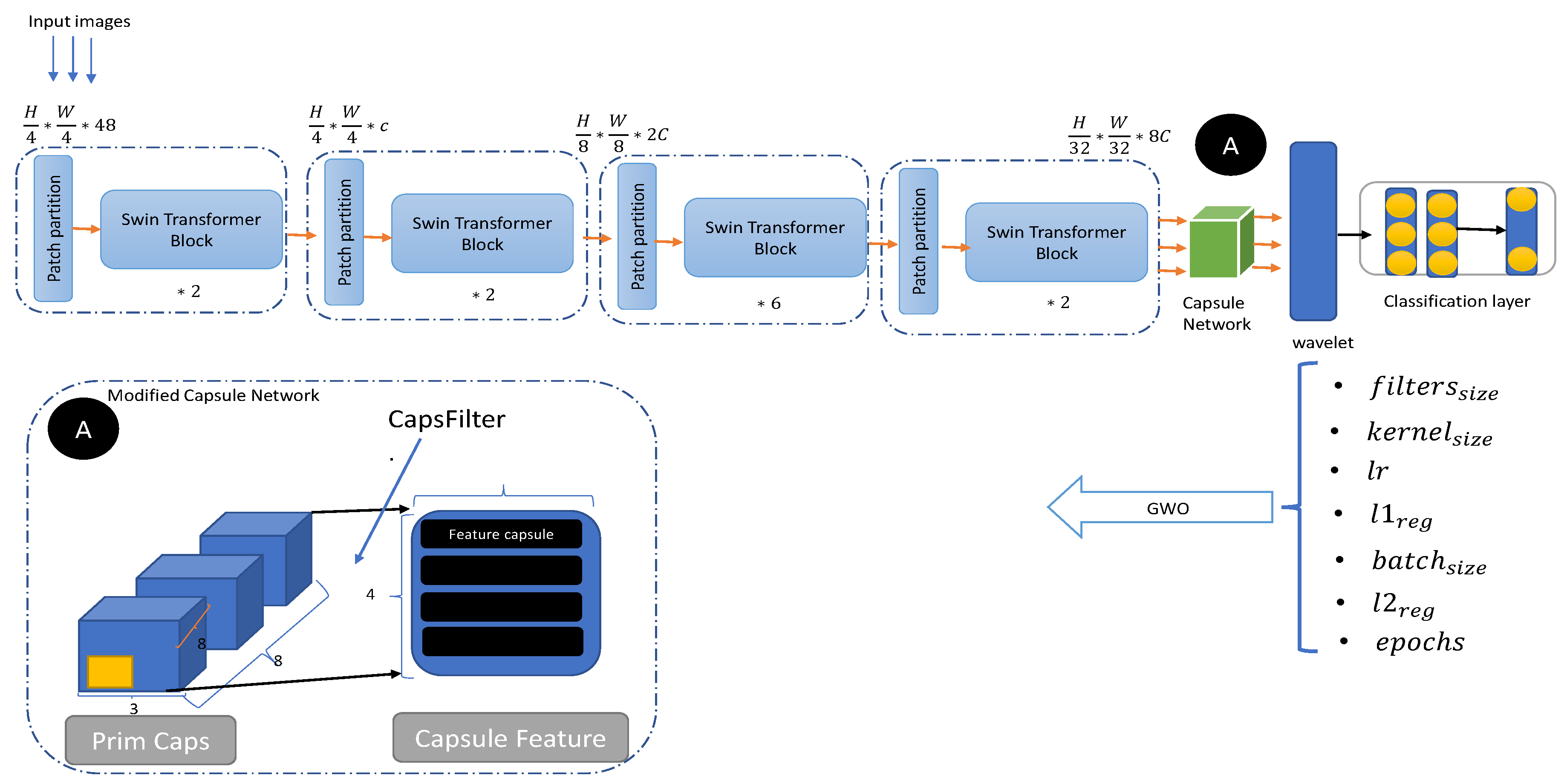
Figure 2.
A sample of data from each class.
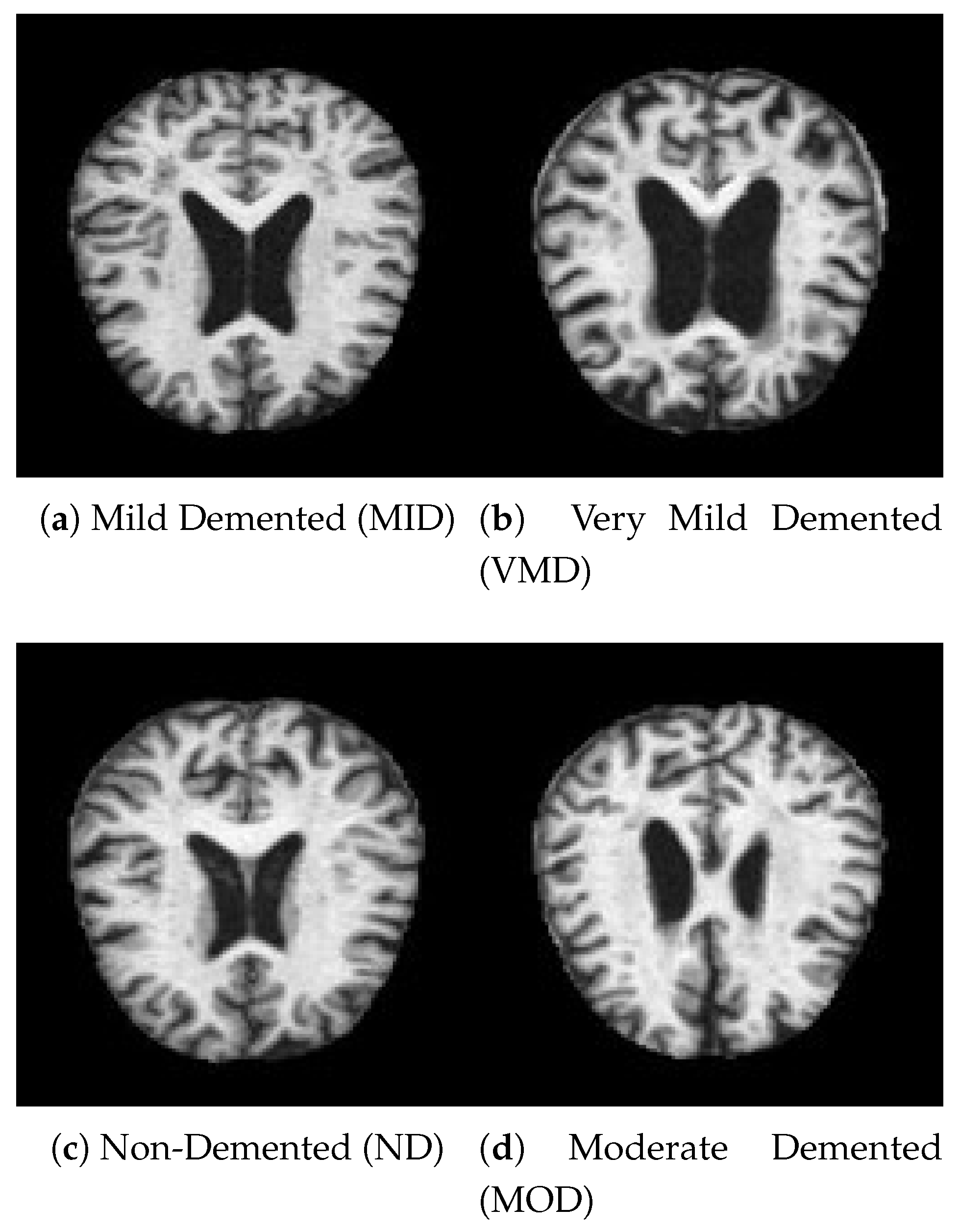
Figure 3.
Bar plot for all classification models on Alzheimer dataset.
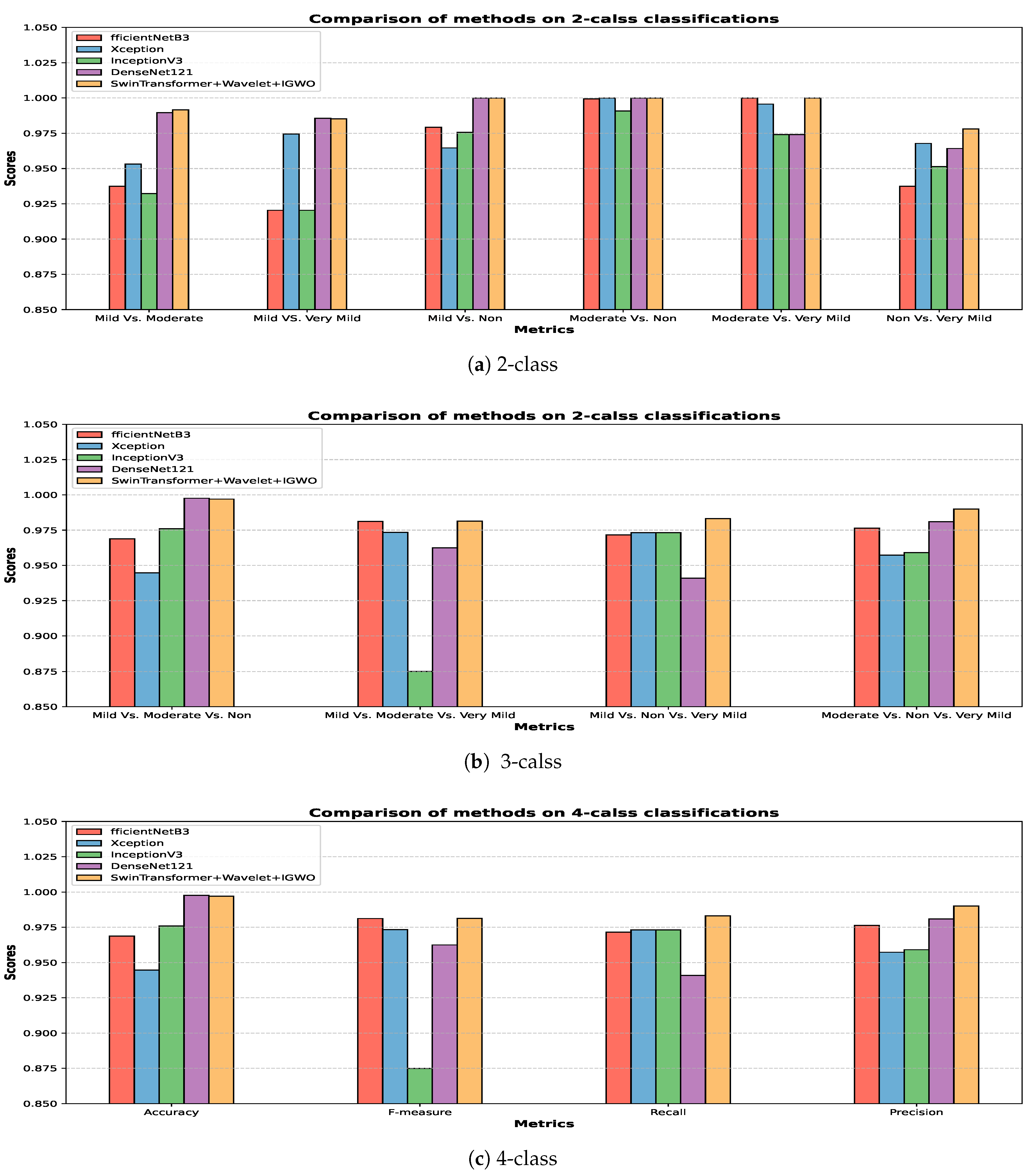
Figure 4.
confusion matrix for four class classification on Alzheimer dataset.
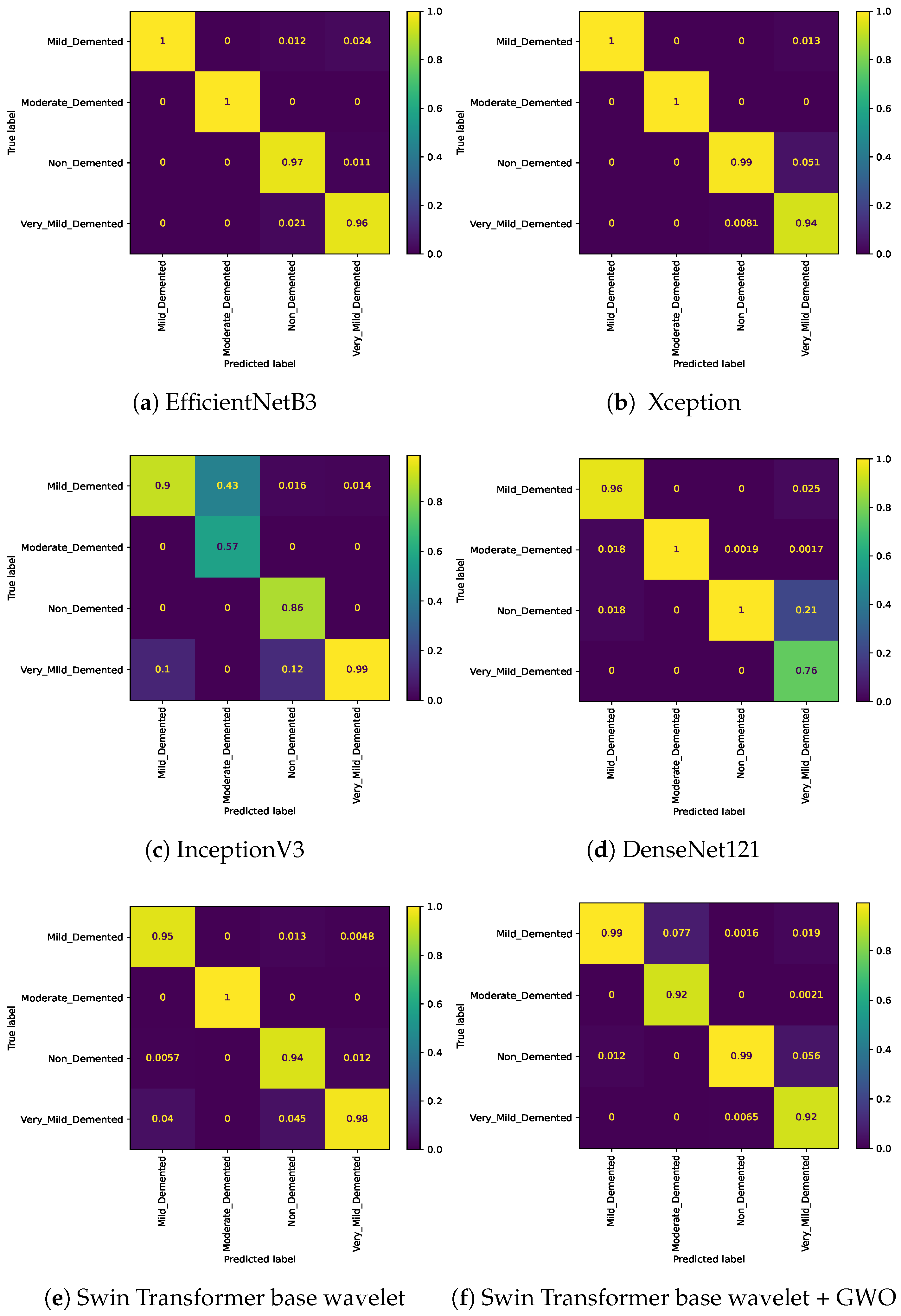
Figure 5.
Confusion matrix for three class (Mild Vs. Moderate Vs. Non) classification on Alzheimer dataset.
Figure 5.
Confusion matrix for three class (Mild Vs. Moderate Vs. Non) classification on Alzheimer dataset.
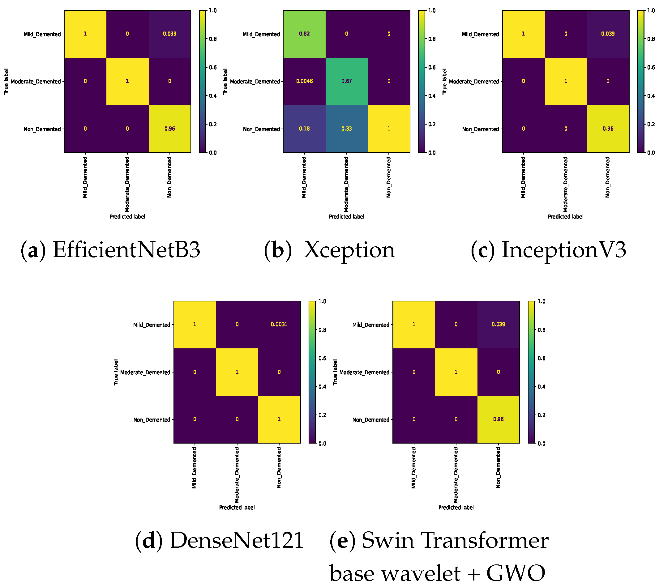
Figure 6.
Confusion matrix for three class (Mild Vs. Moderate Vs. Very_Mild) classification on Alzheimer dataset.
Figure 6.
Confusion matrix for three class (Mild Vs. Moderate Vs. Very_Mild) classification on Alzheimer dataset.
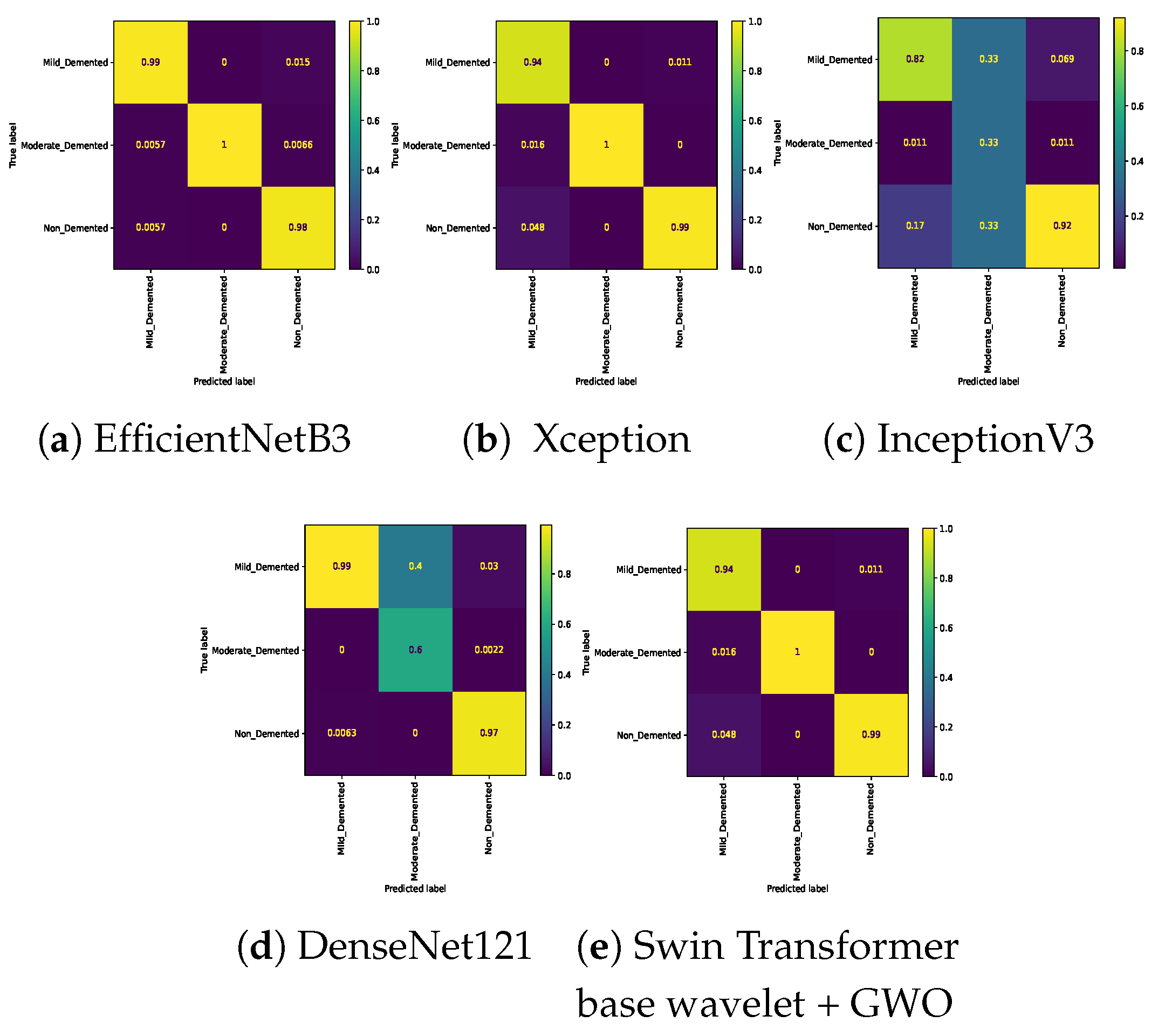
Figure 7.
Confusion matrix for three class (Mild Vs. Non Vs. Very_Mild) classification on Alzheimer dataset.
Figure 7.
Confusion matrix for three class (Mild Vs. Non Vs. Very_Mild) classification on Alzheimer dataset.
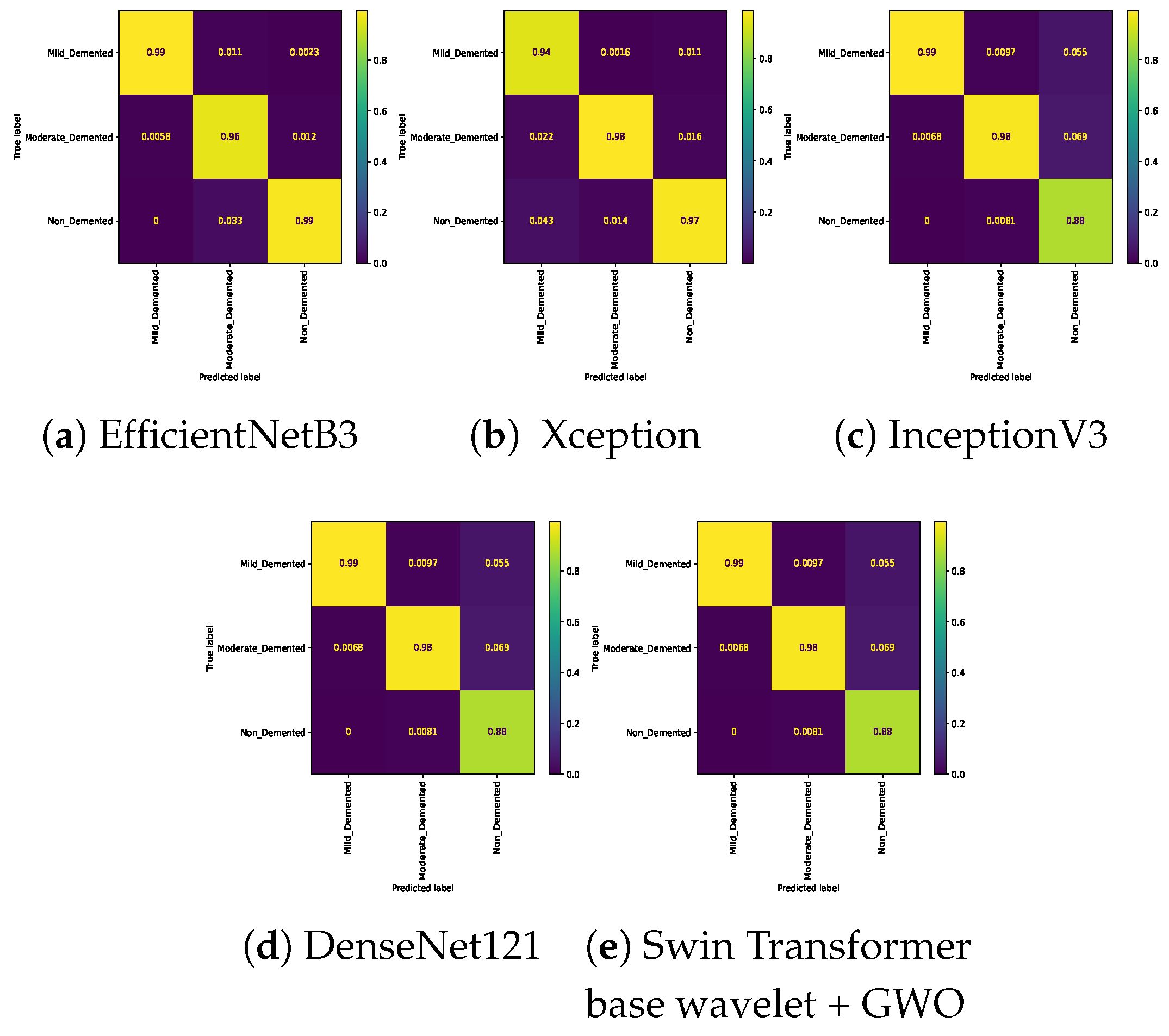
Figure 8.
Confusion matrix for three class (Moderate Vs. Non Vs. Very_Mild) classification on Alzheimer dataset.
Figure 8.
Confusion matrix for three class (Moderate Vs. Non Vs. Very_Mild) classification on Alzheimer dataset.
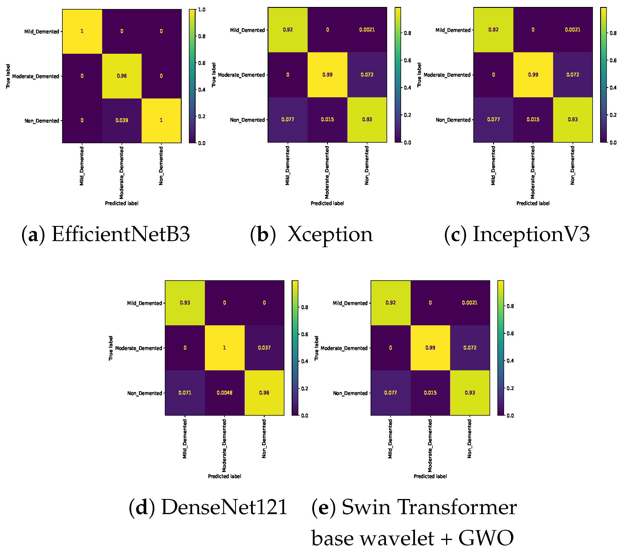
Figure 9.
Confusion matrix for binary classifications (Mild Vs. Moderate) on Alzheimer dataset.
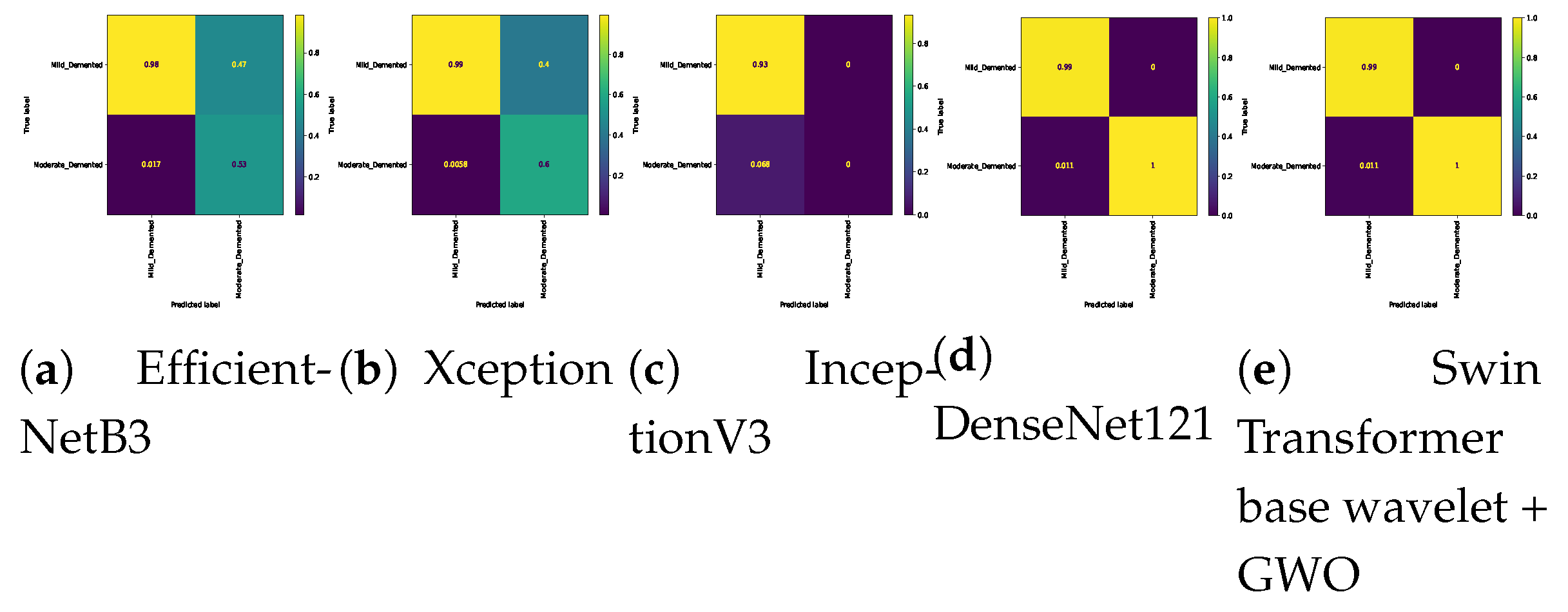
Figure 10.
Confusion matrix for binary classifications (Mild Vs. Very_Mild) on Alzheimer dataset.
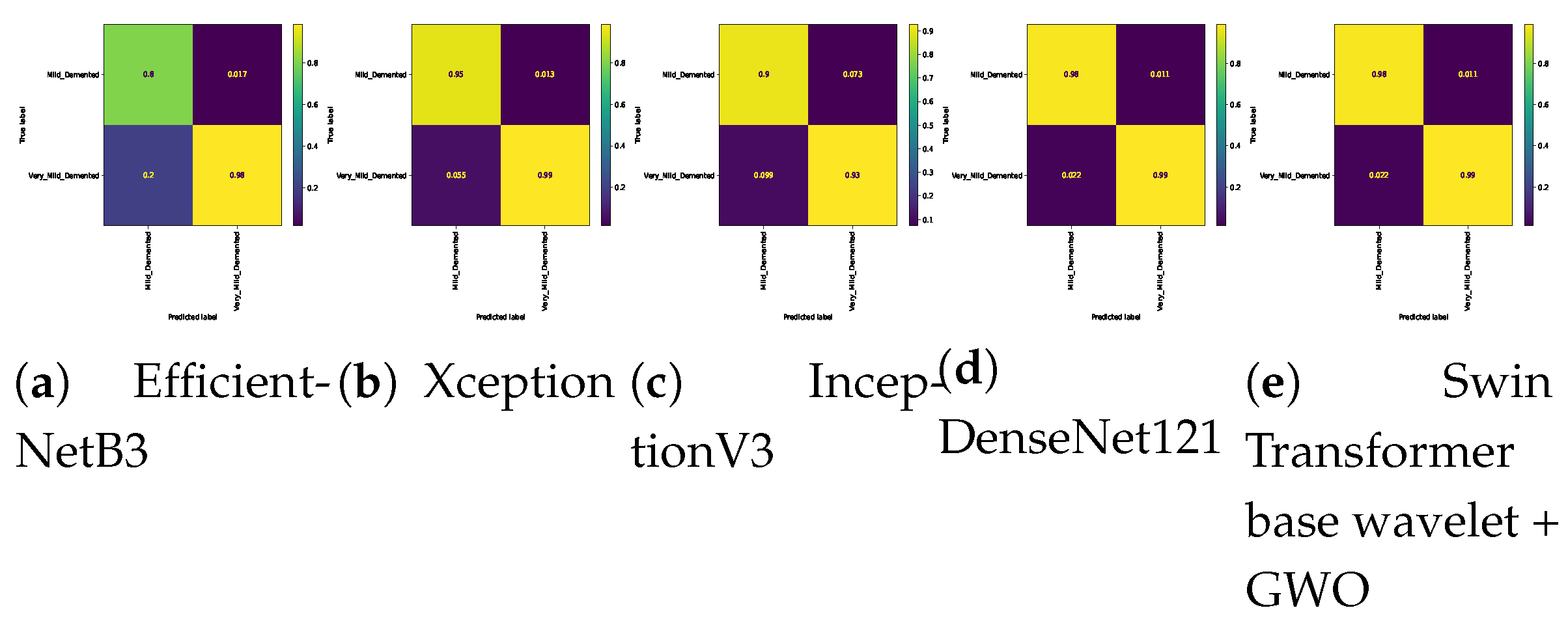
Figure 11.
Confusion matrix for binary classifications ( Mild Vs. Non ) on Alzheimer dataset.
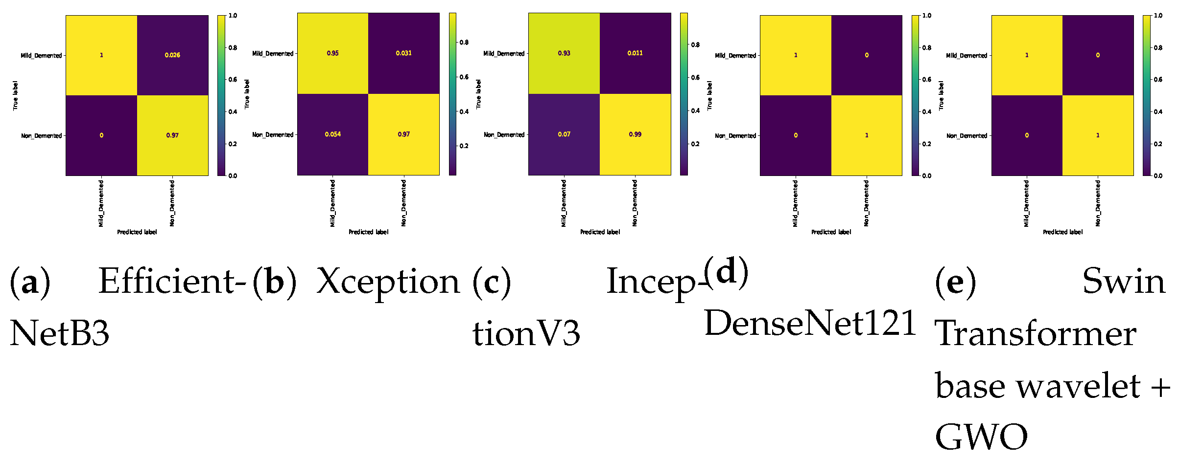
Figure 12.
Confusion matrix for binary classifications (Moderate Vs. Non) on Alzheimer dataset.
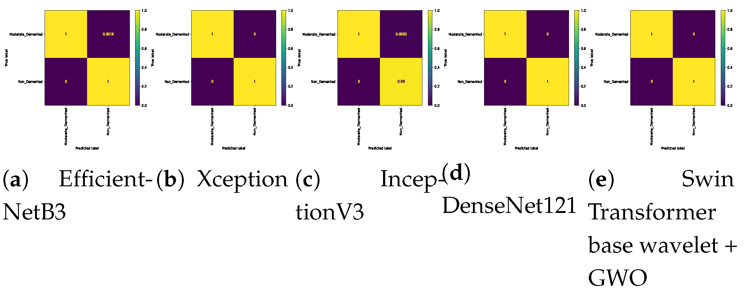
Figure 13.
Confusion matrix for binary classifications (Moderate Vs. Very_Mild) on Alzheimer dataset.
Figure 13.
Confusion matrix for binary classifications (Moderate Vs. Very_Mild) on Alzheimer dataset.
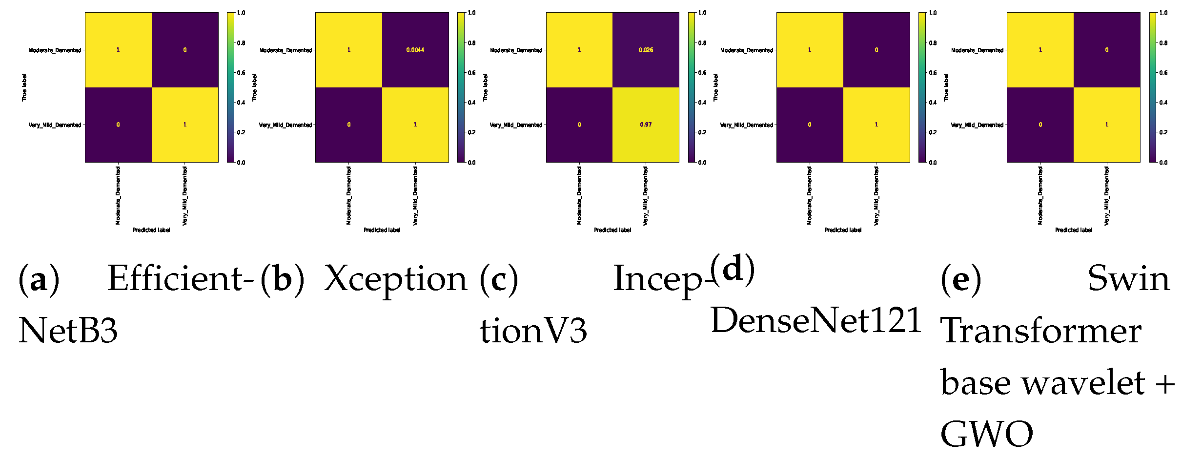
Figure 14.
Confusion matrix for binary classifications (Non Vs. Very_Mild ) on Alzheimer dataset.
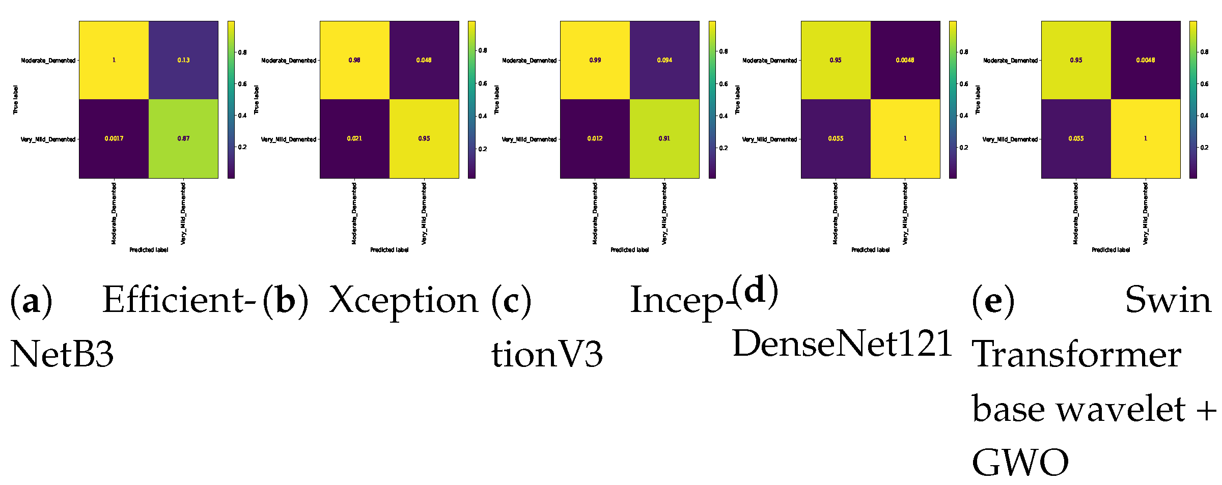
Figure 15.
Number of MRI scans in each class..
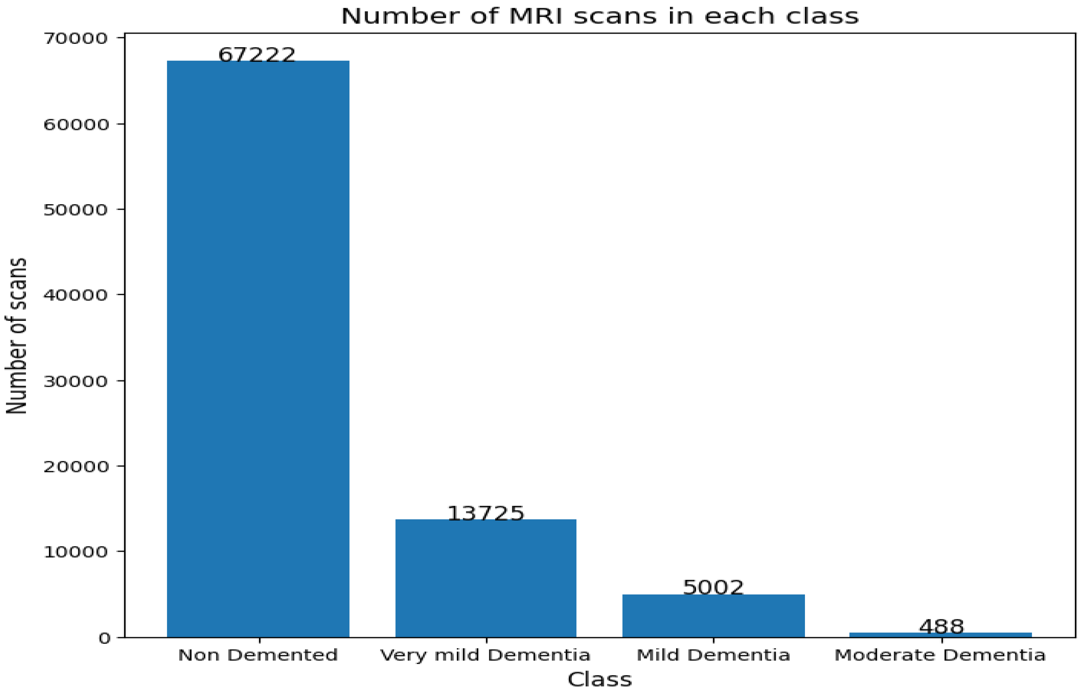
Figure 16.
Number of patients in each class.
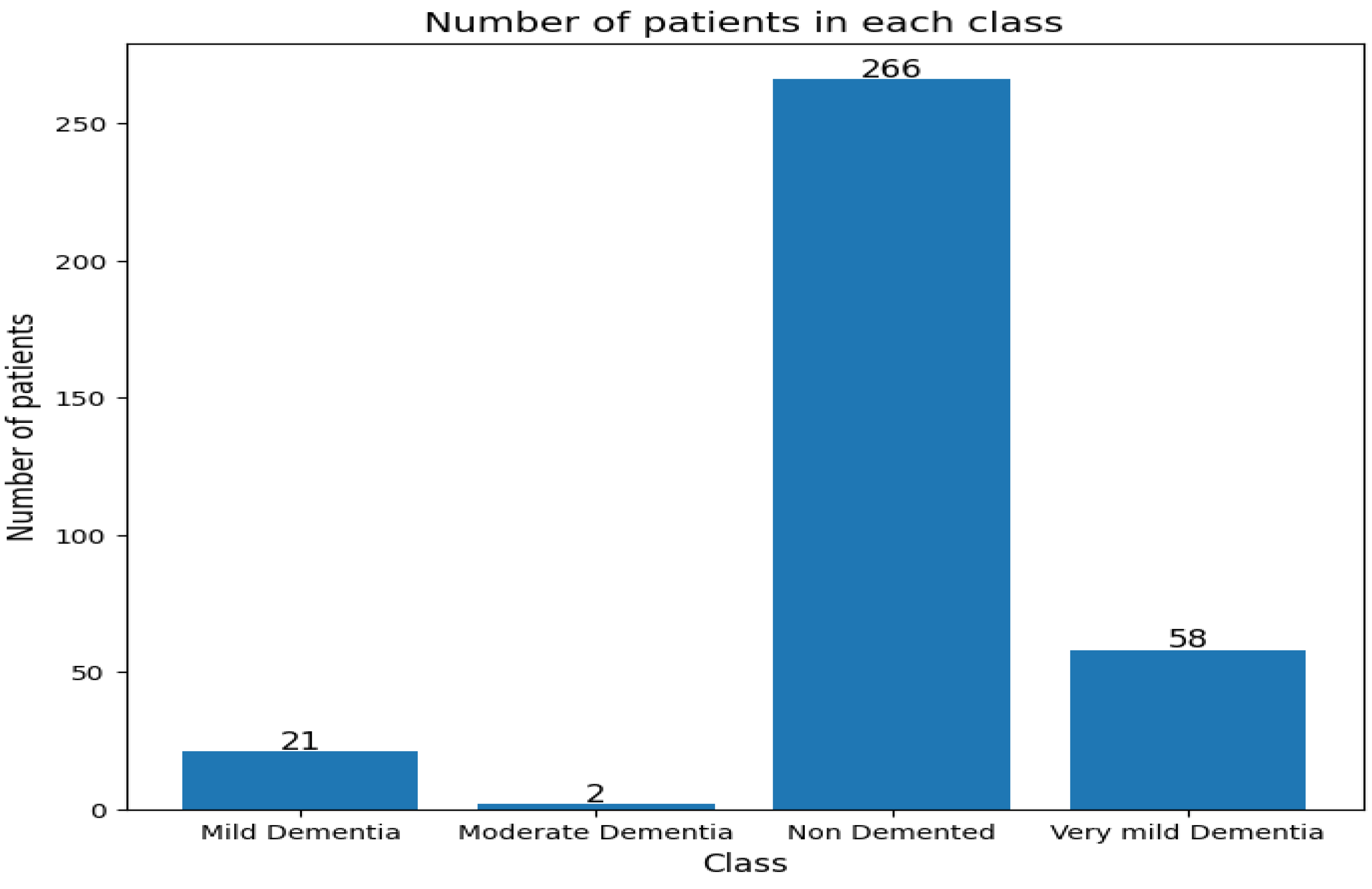
Table 1.
Hyperparameters of the Swin transformer Model Optimized by GWO.
| Optimizer | Lower Bound | Upper Bound |
|---|---|---|
| : filters size | 64 | 128 |
| : kernel size | 3 | 9 |
| lr: learning rate | 0.000001 | 0.001 |
| l2: | 0.0001 | 0.01 |
| l1: | 0.0001 | 0.01 |
| : | 16 | 256 |
| E: epochs | 100 | 200 |
Table 2.
The frequency of images in each class of the dataset before data augmentation.
| Class | Number of Images |
|---|---|
| MID: | 896 |
| MOD: | 3200 |
| ND: | 2240 |
| VMD: | 64 |
Table 3.
The frequency of images in each class of the dataset after data augmentation.
| Class | Number of Images |
|---|---|
| MID: | 4180 |
| MOD: | 1600 |
| ND: | 11200 |
| VMD: | 320 |
Table 4.
Hardware and software requirements for this research.
| Software specifications | ||
|---|---|---|
| Application | version | Description |
| Ubuntu | 18.04.2 | Operating System |
| CUDA | 9.0.176 | Cuda version |
| cuDNN | 7.4.1 | GPU-accelerated library |
| Python | 3.6.7 | Used for coding |
| Keras | 2.2.4 | Neural Network library |
| TensorFlow | 2.12.0 | backend |
| Hardware | ||
| Hardware specifications | Version | |
| CPU | Intel Core i7-12700KF | |
| GPU NVIDIA | geforce gtx 1090 ti | |
| Memory | 16 GB | |
Table 5.
Hyperparameter setting of the tested models.
| Hyperparameter | Values |
|---|---|
| : Batch size | 64 |
| LR: | 0.0001 |
| D: | 0.7 |
| E: Epochs | 100 |
| O: Optimizer | Adam |
| CrossEntropyLoss: Multi class | |
| BCELoss: Binary class |
Table 7.
Three-class classification on Alzheimer dataset. The bold represents the highest results/accuracy achieved for each experiment.
Table 7.
Three-class classification on Alzheimer dataset. The bold represents the highest results/accuracy achieved for each experiment.
| Model | Mild,Moderate, Non | Mild,Moderate, Very_Mild | Mild , Non, Very_Mild | Moderate, Non, Very_Mild |
|---|---|---|---|---|
| EfficientNetB3[42] | 0.9688 | 0.9812 | 0.9716 | 0.9764 |
| Xception[43] | 0.9447 | 0.9734 | 0.9732 | 0.9573 |
| InceptionV3[44] | 0.9760 | 0.8750 | 0.9732 | 0.9591 |
| DenseNet121[45] | 0.9976 | 0.9625 | 0.9409 | 0.9809 |
| Swin Transformer wavelet | 0.9970 | 0.9813 | 0.9831 | 0.9900 |
| Swin Transformer wavelet+ GWO | 0.9980 | 0.9881 | 0.9843 | 0.9912 |
Table 8.
Accuracy of six binary classifications on Alzheimer dataset. The bold represents the highest results/ accuracy achieved for each experiment.
Table 8.
Accuracy of six binary classifications on Alzheimer dataset. The bold represents the highest results/ accuracy achieved for each experiment.
| Model | Mild ,Moderate | Mild , Very_Mild | Mild, Non | Moderate, Non | Moderate, Very_Mild | Non, Very_Mild |
|---|---|---|---|---|---|---|
| EfficientNetB3[42] | 0.9375 | 0.9204 | 0.9793 | 0.9993 | 1.0000 | 0.9375 |
| Xception[43] | 0.9531 | 0.9745 | 0.9646 | 1.0000 | 0.9957 | 0.9678 |
| InceptionV3[44] | 0.9323 | 0.9204 | 0.9756 | 0.9908 | 0.9740 | 0.9513 |
| DenseNet121[45] | 0.9896 | 0.9857 | 1.0000 | 1.0000 | 0.9740 | 0.9642 |
| Swin Transformer wavelet | 0.9916 | 0.9852 | 1.0000 | 1.0000 | 1.0000 | 0.9781 |
| Swin Transformer wavelet+ GWO | 0.9978 | 0.9907 | 1.0000 | 1.0000 | 1.0000 | 0.9798 |
Table 9.
Results for 5-fold cross-validation on 4-class classifications.
| Model | |||||
|---|---|---|---|---|---|
| EfficientNetB3[42] | 0.9512 | 0.9426 | 0.9235 | 0.9543 | 0.9545 |
| Xception[43] | 0.9715 | 0.9694 | 0.9658 | 0.9707 | 0.9713 |
| InceptionV3[44] | 0.9714 | 0.9753 | 0.9669 | 0.9628 | 0.9628 |
| DenseNet121[45] | 0.9632 | 0.9632 | 0.9618 | 0.9747 | 0.9699 |
| Swin Transformer wavelet | 0.9816 | 0.9614 | 0.9708 | 0.9829 | 0.9747 |
| Swin Transformer wavelet + GWO | 0.9875 | 0.9606 | 0.9809 | 0.9797 | 0.9826 |
Table 10.
Statistic and pvalue for four class calssification.
| Model | EfficientNetB3[42] | Xception[43] | InceptionV3[44] | DenseNet121[45] | Swin Transformer wavelet | Swin Transformer wavelet+ GWO |
|---|---|---|---|---|---|---|
| EfficientNetB3[42] | 0.0,1.0 | -4.1328, 0.0033 | -3.5556, 0.0074 | -1.3860, 0.2032 | -3.3544, 0.01002 | -4.8815, 0.00123 |
| Xception[43] | 4.1328, 0.0032 | 0.0, 1.0 | 0.6890, 0.5102 | 2.8305, 0.0221 | 1.2190, 0.2575 | -2.7184, 0.0263 |
| InceptionV3[44] | 3.5555, 0.0074 | -0.6890, 0.5102 | 0.0, 1.0 | 2.2199, 0.0571 | 0.3892, 0.7072 | -2.3053, 0.0500 |
| DenseNet121[45] | 1.3860, 0.2031 | -2.8305, 0.0221 | -2.2199, 0.0571 | 0.0, 1.0 | -1.9801, 0.0830 | -3.7336, 0.0057 |
| Swin Transformer wavelet | 3.3544, 0.0100 | -1.2190, 0.2575 | -0.3892, 0.7072 | 1.9801, 0.0830 | 0.0, 1.0 | -2.8421, 0.0217 |
| Swin Transformer wavelet+ GWO | 4.8814, 0.0012 | 2.7184, 0.0263 | 2.3053, 0.0500 | 3.7336, 0.0057 | 2.8421, 0.0217 | 0.0, 1.0 |
Table 11.
Obtained result on OASIS.
| Model | Accuracy | Precision | Recall | F1 |
|---|---|---|---|---|
| EfficientNetB3 | 0.9898 | 0.9896 | 0.9898 | 0.9897 |
| Xception | 0.9983 | 0.9988 | 0.9988 | 0.9988 |
| InceptionV3 | 0.9981 | 0.9989 | 0.9989 | 0.9989 |
| DenseNet121 | 0.9991 | 0.9999 | 0.9999 | 0.9999 |
| Swin Transformer base wavelet | 1.0 | 1.0 | 1.0 | 1.0 |
| Swin Transformer base wavelet + GWO | 1.0 | 1.0 | 1.0 | 1.0 |
Table 12.
Memory usage, top accuracy, number of parameters, flops of all studied models.
| Architecture | Parameters(10e6) | GFlops | Memory (GB) |
|---|---|---|---|
| EfficientNet | 79.8 | 199.29 | 4.7 |
| Xception | 105.1 | 240.98 | 5.6 |
| IncetionV3 | 144.1 | 321.22 | 5.39 |
| DenseNet121 | 121.7 | 231.1 | 5.35 |
| Swin Transformer wavelet | 155.9 | 401.32 | 5.8 |
| Swin Transformer wavelet+ GWO | 155.9 | 401.32 | 8.2 |
Disclaimer/Publisher’s Note: The statements, opinions and data contained in all publications are solely those of the individual author(s) and contributor(s) and not of MDPI and/or the editor(s). MDPI and/or the editor(s) disclaim responsibility for any injury to people or property resulting from any ideas, methods, instructions or products referred to in the content. |
© 2025 by the authors. Licensee MDPI, Basel, Switzerland. This article is an open access article distributed under the terms and conditions of the Creative Commons Attribution (CC BY) license (http://creativecommons.org/licenses/by/4.0/).
Copyright: This open access article is published under a Creative Commons CC BY 4.0 license, which permit the free download, distribution, and reuse, provided that the author and preprint are cited in any reuse.


