
Submitted:
31 July 2025
Posted:
01 August 2025
You are already at the latest version
Abstract
The two groups of EU economies: the euro area and the non-euro area, are statistically analyzed taking into account the fulfillment of the euro area financial criteria and economic performance over the period 2000-2023. Economic performances and their significant influencing factors, as well as compliance with financial criteria, are presented comparatively for the two groups of countries. Econometric approaches with Error Correction Model (ECM) and Autoregressive Distributed Lag (ARDL) model of the three data panels, including the entire EU, during the analyzed period led to interesting conclusions regarding the existence of economic convergence at the level of the three groups. EU non-euro countries have higher economic growth rates than euro area economies over the period 2000-2023. In the long run, investment brings a higher increase in economic development in EU countries outside the euro area than in euro area countries. The speed of adjustment towards long-run equilibrium in econometric models is slower for non-euro area economies than in the euro area over a one-year period. At the level of the European Monetary Union, change policies have a faster impact on economic development and a faster speed of adjustment towards equilibrium.
Keywords:
economic convergence
; financial criteria
; long-term equilibrium
; short-term model
; speed of adjustment
; cointegration
1. Introduction
Currently, 20 EU countries belong to the Eurozone. On 1 January 1999, 11 European Union countries adopted the euro: Austria, Belgium, Finland, France, Germany, Ireland, Italy, Luxembourg, the Netherlands, Portugal and Spain. The first new member of the Eurozone was Greece on 1 January 2001, and the most recent member of the Eurozone, the 20th, is Croatia on 1 January 2023. Euro area countries have fully implemented the euro-related policies of the Economic and Monetary Union (EMU). On 1 January 1999, the Exchange Rate Mechanism II (ERM II) was established to ensure that volatility in the exchange rates of the euro and other EU currencies does not affect the economic stability of the single market. The Economic and Monetary Union (EMU) provides stability and a sustainable growth across the euro area.
The remaining seven EU countries: Bulgaria, the Czech Republic, Denmark, Hungary, Poland, Romania and Sweden would have to meet the convergence criteria to join the euro area, with the exception of Denmark which obtained a special opt-out from the Maastricht Treaty in 1992. The other six countries are required to adopt the euro when they meet the convergence criteria, including being part of the European Exchange Rate Mechanism (ERM II) for at least two years.
As part of the regular two-year convergence criteria reporting cycle, the European Central Bank and the European Commission examine and review the economic convergence of EU countries in the process of adopting the euro. Their report covers the last ten years and presents the evolution of prices, fiscal balances, the debt ratio, exchange rates and long-term interest rates, as well as other socio-economic indicators important for the integration in the euro area of the remained non-euro EU countries (ECB, 2020).
Denmark meets the conditions for convergence to the euro area, but using the "non-participation clause" in the EU treaties is exempted from the obligation to adopt the euro; it may decide to join Eurozone when decide so.
The 2022 report assessed the sustainability aspects of convergence for each country, except Denmark (ECB, 2022). A common assessment framework is applied to each EU country under review. The report's conclusions aim to achieve strong governance with sustainable public finances to ensure production growth in the medium and long term.
Macroeconomic stability is a prerequisite for sustainable convergence to ensure an efficient business environment. Economic integration with the euro zone allows synchronization with economic cycles.
Our work contributes to the analysis of compliance with the convergence criteria by both euro area economies and non-euro area EU Member States. The conclusions underline the importance of respecting the financial convergence criteria to ensure the economic convergence of EU countries. Another contribution is econometric approaches to explain EU economic convergence influenced by national debt management and investment decisions, for the euro area, the EU area outside the euro area, as well as at the EU level.
Our study presents the statistical situation of the Eurozone economies, as well as those outside the EU euro area, for each financial criterion. Compliance with financial criteria ensures economic growth. Testing the existence of a long-term relationship attests to the economic convergence of economic growth and investment and debt strategies. For both groups, as well as at the EU level, economic growth is mainly influenced by the same factors. Our econometric models explain the different influences on GDP growth, in different situations. Testing the significance of differences between the model coefficients provides information about economic convergence and the way and group level at which it operates.
2. Literature Framework and Working Hypotheses
The public debt of Eurozone countries, its dynamic stability and its nonlinear behavior on economic growth were research subjects for many economists (Baum et al., 2012; Cao et al., 2024; Checherita-Westphal & Rother, 2010; De Soyres et al., 2022; Katsikas et al., 2023; Lagoa et al., 2022).
The economic convergence in euro based economies was studied by many authors (Haynes & Haynes, 2016; Quiroga, 2007; Vojinović et al., 2010; Yin et al., 2003).
The sustainability of public debt (World Bank & IMF, 2001) was also analyzed in the context of a long-term relationship with the economic growth and the financial criteria by Menuet and Villieu (2014), and by Rao Aiyagari and McGrattan (1998).
Our paper analyzes the economic convergence of both the euro area and the non-euro EU area, based on the existence of a long-run relationship between GDP and the debt/GDP ratio, investment and openness. The convergence in the post-communist economies was studied by Vojinović et al. (2010) and by Vratislav (2009).
Our paper envisages and characterizes the economic convergence as a “dynamic and multivariate concept” (Haynes & Haynes, 2016). The concept of convergence involves multiple cross-sections, analyzed over a period of time; it is also a dynamic and spatial concept. The multivariate aspect takes into account the number of explanatory variables of the countries considered at the level of the studied group.
Economic convergence is described by the long-term relationship between GDP and its significant influencing factors in a given area. The dynamic character is given by the time-varying nature of the long-term relationship under different economic shocks.
The process of economic integration is based on specific objectives and accepted rules to ensure economic convergence (Quiroga, 2007). Compliance with the financial criteria for joining the euro area ensures EU economic convergence.
The financial criteria for joining the euro area were established by the Maastricht Treaty of 1991. Every two years, the financial convergence criteria for joining the euro area are assessed and updated in Convergence Reports by the European Commission and the European Central Bank.
The two last Convergence Reports of 2020 and 2022 with reference periods April 2019 to March 2020 and May 2021 to April 2022, respectively set the reference value for price stability criterion of 4.9%, the reference value of the 2022 Convergence Report (1.8% of the 2020 Convergence Report). The inflation rate over one year cannot be higher than 1.5 percentage points above the rate of the three best performing Member States.
Sound and sustainable public finances presuppose compliance with the following budget deficit and public debt conditions:
- -
- The criterion of the government's budgetary position according to which the deficit/GDP ratio is less than 3% of GDP. Candidate countries for the euro area cannot be in the excessive deficit procedure; Romania is the only country in this situation until 2024;
- -
- Gross public debt (percentage of GDP) should be lower than 60%.
The exchange rate criterion, for the stability of exchange rates of the national currency and the euro requires that the countries entering the euro area should participate in Exchange Rate Mechanism II for at least two years.
The long-term interest rate criterion of 2.6%, the reference value of the 2022 Convergence Report (2.9% of the 2020 Convergence Report). The long-term interest rate should not be more than 2 percentage points above the rate of the three best performing Member States in terms of price stability.
Economic convergence must be followed by legal convergence. Legal convergence assumes the corresponding legal alignment with the EU legislation related to the National Central Banks.
Our study analyzes the state of compliance with the euro area financial criteria by all EU member states' economies and provides an analysis of economic development through statistical and econometric methods in Section 4.1.
The objectives of the study can be summarized in two sets of hypotheses: one to attest to the existence of economic convergence of groups of countries, and the second to explain some general characteristics of the convergence mechanism.
The hypotheses regarding the existence of economic convergence are:
H1:
There is economic convergence between the countries in the euro area.
H2:
There is economic convergence of EU countries outside the euro area.
H3:
There is economic convergence between EU countries.
The hypotheses that describe the characteristics of the convergence mechanism are:
H4:
Economic growth rates are higher in economies outside the euro area than in those within the euro area.
H5:
Investments are the engine of economic development.
H6:
The more developed the level of the organizational entity, the faster the speed of adjustment towards equilibrium.
These hypotheses are verified by the results of statistical analyses and econometric models in Section 4.2 of our paper. The conclusions are formulated in Section 5.
3. Materials and Methods
3.1. Data and Variables
The data for the euro area form a long panel, consisting of twenty countries, and the period analyzed is twenty-three years. The panel data for non-euro area EU countries covers seven countries for the same period, also being a long panel. The following variables were collected from EUROSTAT and were used in the proposed econometric models (Mbaye et al., 2018). Some of these variables were calculated to verify compliance with the convergence criteria through various statistical and econometric methods:
CPI – Consumer Price Index (%) with fixed base in 2015,
RINFL – inflation rate (%),
LIM_AVG_RINF – upper limit allowed for accepting price stability (%),
CAB_GDP - current account balance as a percentage of GDP (%),
DEBT_GDP - debt-to-GDP ratio (%),
REXCH – annual changes (%) of exchange rates,
REXCH2015 - annual data of real effective exchange rates (REER) (deflator: consumer price index - 20 trading partners - euro area from 2023), as dynamic indices with fixed base in 2015,
LONG_INT_R – long-term interest rate (%),
LIM_LONG_INTR - average performance limit of the three best-performing Member States plus 2 percentage points,
GDP - real Gross Domestic Product (mil. euro 2010),
LN_GDP – logarithm of the real Gross Domestic Product,
YRGDP – yearly dynamic rate of GDP (%),
OPN – ratio of commercial flows of Imports plus Exports as percentage in GDP (%),
GFCF – investments, as real Gross Fix Capital Formation (mil. euro 2010),
GFCF_GDP – ratio between Gross Fix Capital Formation and GDP (%).
The interpretation of the results and the conclusions of the study compare the degree of compliance with the financial criteria by the two groups of EU countries. The study analyses the economic convergence of the euro area, non-euro area and EU countries and shows that this is ensured by compliance with the euro area financial criteria.
3.2. Statistical Analysis and Econometric Models
Considering both groups of euro area and non-euro area Member States, it shows the better positions of euro area countries compared to other EU countries and highlights the advantages of membership of the euro area and the European Monetary Union (EMU).
Graphical analyses of the evolution of convergence indicators and comparisons with the upper limits calculated for each criterion each year allow conclusions to be drawn regarding the positions of countries and their efforts to meet the convergence criteria.
The analysis of compliance with the convergence criteria is based on comparing the evolution graphs of the indicators with certain permitted limits. These limits can be fixed, such as 60% for the debt-to-GDP ratio, 3% for the budget deficit, or variable limits calculated as the average level of the three best-performing countries in the euro area, which differ from year to year, in the case of price stability and of the long-term interest rate.
We used the simple correlation coefficient to analyze the compliance of the actual indicators with the price stability and the long-term interest rate criteria in the European Union. This analysis was carried out by sub-periods and for the entire period, both for the euro area and for the EU countries outside the euro area.
We used the independent samples t-test for equality of means, in the SPSS program, to assess compliance with the exchange rate stability criterion in the euro area and in EU countries outside the euro area. We conclude that, by removing Denmark and Sweden from the group of non-euro area countries, the test for equality of means shows higher volatility in the non-euro area and significant differences compared to the exchange rate variation in the euro area.
In SPSS we used one-sample t-tests for the 95% confidence intervals of the variation of the exchange rate means for all EU countries and three groups of EU countries: the euro area group, the non-euro area group and the non-euro area group without Denmark and Sweden. The results lead to the conclusion that the non-euro area group, excluding Denmark and Sweden, had higher volatility and higher confidence interval values.
The econometric approach to GDP evolution, using its logarithmic expression through LN_GDP, (denoted by yit, where i is the country and t is the year), both in the euro area and outside the euro area, considers as explanatory variables those that are directly influenced by the financial convergence criteria.
Correlation analysis, Granger causality analysis and panel cointegration tests suggested the following explanatory variables (xit , with i – country and t - year): investment dynamics through LN_GFCF, the debt-to-GDP ratio, called DEBT_GDP, and the international openness, OPN, as the ratio between the sum of imports and exports and GDP.
The GDP variable is dynamic depending on its own past values, being persistent, and the regressors are not strictly exogenous.
Long-term equilibrium represents the economic convergence of the groups of countries analyzed: Eurozone, EU non-euro area and at EU level.
Unobserved heterogeneity, heteroscedasticity, and autocorrelation of residuals along cross-sections—that is, within countries but not across them—are addressed by using Generalized Method of Moments (GMM) panel models (Mehrhoff, 2009). When the GMM Difference estimator can produce a biased and inefficient estimate (Blundell & Bond, 1998) of the coefficient of the lagged dependent variable, then the problem is solved by System GMM. But the GMM system proposed by Arellano and Bover (1995) is used for the short panel.
When handling long panels, ECM (Error Correction Models) and ARDL (Autoregressive Distributed Lag) models can provide a dynamic approach. The existence of a long-run equilibrium supported by the cointegrating relationship of the variables is identified together with the short-run behavior. We can use both Error Correction Models and ARDL models.
If the variables y and x in the Fixed Effects (FE) model (eq. 1) are integrated of the same order I(1) and the residuals are stationary I(0), then the variables are cointegrated. They tend to a long-run equilibrium, and eqn. (1) is the long-run model. The residuals in equation (1) represent the error correction term (ECT), whose one lagged value is used in the short-run model in equation (2), called Error Correction Model (ECM).
If the coefficient of the ECT term equation (3) in the ECM (equation 2) is negative and significant, then there is a long-run equilibrium, and the coefficient is the speed of adjustment towards equilibrium over a one-year period, for the countries in the group.
The ARDL approach of Mean Group (MG) and Pooled Mean Group (PMG) can also explain long-term and short-term developments. An advantage of PMG/ARDL method is that in the short run equation it allows the coefficients to differ from country to country equation (4). The PMG estimator constrains the long-run coefficients to be identical, but allows the short-run coefficients and the variance of the residuals to vary across countries. The coefficient in equation (4) is the speed of adjustment towards equilibrium over a one-year period, for each country i.
The long-run model with the same cointegrating coefficient, represents the economic convergence, specific for each analyzed group of countries in euro area and non-euro area.
4. Results and Discussion
Our study aims to characterize and compare the state of economic convergence of both types of EU countries, belonging to the euro area and those outside the euro area, by analyzing compliance with financial convergence criteria depending on economic conditions.
With accession to the Eurozone, the EU's economic convergence will ensure the well-being of all its member countries.
4.1. Compliance with Financial Convergence Criteria in the Euro Area and Outside the Euro Area in the Period 2000-2023
The convergence criteria are a set of requirements regarding macroeconomic indicators that EU member states must meet in order to join the euro area. The economic criteria refer to price stability, sustainable public finances, exchange rate stability and stable long-term interest rates.
The analysis of the compliance status of both groups of EU countries for each criterion highlights the differences in financial performance between the euro area and non-euro area. Meanwhile, membership in the Eurozone offers advantages for a more developed and stronger European Union. Economic differences between EU member states give countries that do not comply with the convergence criteria an inferior status, but also a reason to comply with them.
4.1.1. Price Stability Criterion in the Period 2000-2023
The chart in Figure 1 shows for both groups of EU Member States the evolution of the Consumer Price Index (CPI) over the period 2000-2023, with fixed base in 2015. The upward trend is steeper over a larger range for countries outside the euro area than for the euro area.
The average annual change in the CPI, in Figure 2, highlights two sub-periods for the two areas. The first sub-period, 2000-2008, shows some stability with constant changes in the CPI for the euro area, and a more volatile downward trend for non-euro countries.
The second sub-period 2009-2023 shows a similar evolution of the average inflation rates for both groups, but with higher values for non-euro economies. The impact of the 2008 economic crisis produced a deeper CPI decrease in 2009 for the euro area than for non-euro area countries. The inflation rate in 2020 was close to 0 for the euro area, while it was around 2% in non-euro EU countries. Russia's war against Ukraine, which began in 2022, led to a major change in the CPI of around 10% for the Eurozone and over 12% for non-euro countries.
The average of the annual inflation rates of the three best-performing Member States in terms of price stability, plus 1.5 percentage points, represents the upper limit of the convergence criterion on price stability; this is referred to as LIM_AVG_RINFL in Figure 2. In terms of price stability, the three best-performing Member States are those with the smallest variations in the CPI, called RINFL, and these differ from year to year.
In Figure 2, the average inflation rate (RINFL) in the euro area countries exceeds the admissible limit of the convergence criterion on price stability in the years 2007-2010 and 2021-2023; the major causes of the price increase being: the economic crisis in 2008 and after the COVID-19 pandemic in 2020, and the Russian-Ukrainian war in 2022. The 1.8% inflation reference value set by the 2020 Convergence Report was met only in that year. The 2022 Convergence Report increased the inflation benchmark to 4.9%, but it was underestimated because the Russian war that began in February 2022 triggered price increases.
For EU countries outside the euro area, the average inflation rate was below the upper permissible limit only in the years 2013-2017; above the reference value of 1.8% in 2020 and much more in 2022 and 2023. The inflation rate (RINFL) was calculated based on fixed-base CPI’s in 2015. The summary data on the inflation rate to be taken into account for the price stability criterion are presented in Table 1, for both the euro area and the non-euro area.
In Figure 3, especially in the second sub-period 2009-2023, after the 2008 economic crisis, almost all euro area countries managed to comply with the price stability criterion, but in the last two years 2022-2023, and especially in 2022, some countries violated it: Estonia, Latvia, Lithuania, Slovakia, Croatia, and the Netherlands.
In Figure 4, starting in 2009, non-euro area EU countries managed the price stability criterion differently until 2021, when the price boom changed the upward trajectory of the inflation rate over the allowed limit. Denmark and Sweden have almost fully fulfilled the price stability criterion, but represent special cases through their formal decision to postpone joining the euro area. Romania, and especially Hungary, had problems during the analysis period in respecting price stability, being above the admissible limit of this criterion in almost all years.
By analyzing the correlation (r – simple correlation coefficient) between the inflation rate and the upper convergence limit for this criterion, in Table 2, we can assess the intensity of compliance by the two groups of EU countries with convergence in price stability.
We see in Table 2 that price stability was gradually achieved after the establishment of the euro area in 1999. Before the 2008 economic crisis, weak convergence for euro area countries corresponded to a complete lack of convergence for EU countries outside the euro area.
In the period 2009-2023 the euro countries were in strong compliance with the price stability criterion, and this was also the case for non-euro EU countries. Considering the entire period analyzed, we observe strong compliance for the euro area and medium compliance in price convergence for the non-euro EU area.
4.1.2. Budget Deficits and Public Debts in the EU in the Period 2000-2023
The summarized data of the two indicators to be taken into account for the budgetary criteria are presented in Table 3, both for the euro area and for the non-euro area: the current account balance as a percentage of GDP (CAB_GDP) and the debt/GDP ratio (DEBT_GDP).
To achieve sustainable public finances, two requirements must be met: a deficit/GDP ratio below 3% and a gross public debt/GDP ratio below 60%. Figure 5, Figure 6, Figure 7 and Figure 8 reflects how both budgetary criteria were met in the period 2000-2023.
After the 2008 crisis, since 2009, both euro area and non-euro area countries have respected on average above -3% for the current account balance as a percentage of GDP (denoted by CAB_GDP), with the exception of the non-euro area excluding Denmark and Sweden. If we consider these two countries, the non-euro area also meets this criterion.
We do not consider Sweden and Denmark in the graph in Figure 5 (right) because they had surplus balances in the period 2000-2023, as seen in Figure 6. They have already met the economic convergence criteria, and joining the Eurozone is their option. The year 2022 was a difficult one for almost all EU non-euro countries, except for Denmark and Sweden.
In Figure 6 we see Denmark and Sweden with budget surpluses, a positive balance in the analyzed period. Only Hungary and Romania had deficits in 2023. Bulgaria, Poland and the Czech Republic made efforts to maintain the budget balance higher than -3%.
Looking at public debt as a percentage of GDP, in Figure 7, we see that euro area countries have a significantly higher debt-to-GDP ratio compared to non-euro area EU countries.
Euro area countries benefit from the governance framework of EMU policies. Since 2009, the 60% threshold has been exceeded, on average, by all euro area countries. To compare with the euro area group, we kept the same limits of the graph to see the right place in terms of the size of the average debt-to-GDP ratio for the seven non-euro countries. Considering the debt-to-GDP ratio for each non-euro EU country in Figure 8, we note that only Hungary did not meet the criterion; starting with 2005 and for the rest of the period, it was above the 60% limit.
With the exception of Hungary, all other EU countries outside the euro area comply with the debt criterion over the period 2000-2023. Non-euro countries would have to meet both budgetary requirements imposed by the convergence criteria to join the euro area.
4.1.3. Exchange Rate Criterion in the Period 2000-2023
Using annual data of real effective exchange rates (REER) (deflator: consumer price index - 20 trading partners - euro area from 2023), as dynamic indices with fixed base in 2015 (REXCH2015), we find the annual changes (%) of exchange rates (REXCH). The statistical summary of the annual changes (%) in exchange rates is presented in Table 4 for the period 2000-2023 for the euro area and for the non-euro area.
The standard deviation is smaller for the REXCH in the euro area than for the non-euro EU countries. There is a larger variation in exchange rates for the non-euro EU countries, as can also be seen in Figure 9.
We observe a small range of variations in the real effective exchange rate for euro area countries, especially over the period 2009-2023. For non-euro area EU countries, the 2000-2010 sub-period recorded high volatility, compared to the following sub-period 2011-2022, which is characterized by a certain stability of exchange rates.
To test whether annual exchange rate changes are significantly different for the euro area and the EU outside the euro area, we use the independent samples t-test for equality of means, using SPSS software, as shown in Table 5. Levene's test for equality of variances accepts the hypothesis of equal variances with a significant p-value (Sig.) <1%. In this situation, the t-test gives a calculated t-value less than the theoretical t-value for 619 degrees of freedom (dl) with a p-value of Sig. (two-sided) > 5% accepting the null hypothesis of the two-sided test of equality of means. The 95% confidence interval of the difference in means changes sign from minus to plus, meaning that the interval contains the value 0 and that the two means may be equal. The conclusion is that, in terms of exchange rate stability, the difference between the averages of the two groups of countries is not significant.
We remove Denmark and Sweden from the group of non-euro countries and repeat the test for equality of means, comparing the euro area with the updated group of non-euro countries without Denmark and Sweden.
In Table 6, the F-statistic of Levene test recognizes equal variances, and the corresponding t-statistic with a significance Sig. < 1% rejects the null hypothesis of equal means. The negative difference between the means belongs to a negative interval with probability 95%, which preserves the sign.
The conclusion is that the very good situations of Denmark and Sweden change the analysis when they are taken into account in determining compliance with this criterion. When we consider them (Table 5), it seems that there is a convergence of exchange rate stability between the two areas, but, in reality (Table 6), there is no convergence between the euro area and the euro area candidate countries in terms of the exchange rate criterion.
Table 7 contains the one-sample t-tests for the 95% confidence intervals of the REXCH means for the three groups of EU countries and for the entire European Union, all of which are significant at Sig.<5%.
The conclusion regarding the stability assurance is that the EU countries outside the euro area still have to face this criterion. In Table 7 we see that the REXCH standard deviation and the mean standard error are larger than for the euro area. The confidence interval of the average exchange rate changes has a higher upper limit than that of euro area range. If we consider the non-euro area, without Denmark and Sweden, as the two developed countries have already met the convergence criteria, the results tilt upwards. The average annual exchange rate variations, as well as the standard deviation and standard error, are much larger than those of the euro area. The 95% confidence interval is larger, with its limits being higher than those corresponding to all other confidence intervals. The wider range of exchange rate fluctuations is determined by its higher volatility.
This criterion is not met by the group of countries outside the euro area, excluding Denmark and Sweden. In addition, countries must have participated in the European Exchange Rate Mechanism (ERM II) for at least two years.
4.1.4. The Long-Term Interest Rate Criterion in the Period 2000-2023
The statistical summary of the long-term interest rate (LONG_INT_R) of the countries in the three situations for the euro area, the non-euro area, and the non-euro area excluding Denmark and Sweden, as well as the corresponding admitted limit for the long-term interest rate criterion (LIM_LONG_INTR) are presented in Table 8.
The upper limit of the criterion for each year is the average of the minimum long-term interest rates of the three best-performing euro area countries, which differ from year to year.
Euro area countries have the same average intensity of compliance with the long-term interest rate criterion in the sub-periods of the 2000-2023 period.
The non-euro area is in full compliance with this criterion, after the 2008 economic crisis, but thanks to the two developed countries, Denmark and Sweden, which modify the conclusion regarding the efforts of the other countries outside the euro area.
The non-euro area, excluding Denmark and Sweden, is in weak compliance in the first sub-period 2000-2008 and then in medium compliance for the second sub-period and for the entire period.
The long-term interest rate criterion is respected, on average, by euro area countries, as shown in Figure 10 (left). For EU countries outside the euro area, the impact of the 2008 economic crisis and Russia's war in Ukraine in 2022, led to an increase in the average long-term interest rate since 2008, above the average performance limit of the three best-performing Member States, plus 2 percentage points, as shown in Figure 10 (right).
Denmark and Sweden met the criterion, as seen in Figure 11, and taking them into account could change the conclusion regarding compliance with this criterion by non-euro countries (Table 9).
EU countries that are not part of the euro area must respect this criterion and, as seen in Figure 11. Hungary, and especially Romania, did not comply with it, both being placed above the upper limit allowed for the long-term interest rate.
4.2. Convergence of Economic Development in European Union in the Period 2000-2023
4.2.1. Evolution of GDP per Capita in Euro and Non-Euro Area in the Period 2000-2023
To characterize economic development, we analyze the evolution of GDP per capita in constant prices 2010 and the annual changes in this indicator for both the euro area and outside the euro area. We removed Denmark and Sweden from the group of non-euro area EU countries; their very good performance could affect the conclusions regarding the status of EU countries to join the euro area.
In Figure 12, the difference in the size of GDP per capita in Eurozone countries compared to non-euro EU countries is evident. The two shocks of the 2008 economic crisis and the 2020 pandemic had a greater impact on GDP per capita in Eurozone economies than in those outside the zone.
Annual variations in GDP per capita are larger and more volatile in the period 2000-2008 in EU countries outside the euro area, and the recovery after the crisis is much faster, with higher dynamic rates than in the euro area.
4.2.2. Modeling Economic Convergence in Euro Area Countries in the Period 2000-2023
Economic convergence in EU countries is seen as a common direction of long-term GDP development, as a macroeconomic indicator characterizing the overall development performance of the EU.
All efforts to meet the convergence criteria are reflected in the size of GDP and its dynamics. All convergence criteria are global indicators that have a national level of determination, and the use of GDP instead of GDP per capita provides a better understanding of economic dynamics at the national and macroeconomic level of the EU. We use the logarithmic expression of GDP, denoted LN_GDP, which allows the interpretation of annual changes as its dynamic rates. Price stability ensures a balanced and predictable business environment. More stable exchange rate variations have positive effects on the efficiency of international trade flows, expressed by the international openness indicator, denoted by OPN. The long-term interest rate determines the basic mechanism of investments, expressed by the Gross Fixed Capital Formation indicator, which is used here as a logarithm and denoted by LN_GFCF. The national capital structure characterized by budgetary constraints is represented by the debt-to-GDP ratio, denoted as DEBT_GDP.
Considering the intensity and nature of the correlations between the variables LN_GDP and DEBT_GDP, LN_GFCF and OPN, we conclude that the results are similar for both sub-periods, before and after the 2008 economic crisis, as well as for the entire period presented in Table 10.
During the analyzed period, the GFCF indicator had a very strong and positive correlation with GDP. Debt-to-GDP ratio had a weak and positive correlation with GDP. International openness (OPN) had a weak and negative correlation with GDP, as well as a weak and negative correlation with investment and the debt-to-GDP ratio. In Figure 13, the evolution of the macroeconomic indicators considered in our econometric approach shows upward trends over the period 2000-2023.
In Table 11, the Granger causality analysis reveals differences according to the sub-periods 2000-2008 and 2009-2023 and compared to the entire period 2000-2023.
The medium intensity conformity of the long-term interest rate criterion in the three periods, in the euro area (Table 9), determines LN_GDP to be Granger cause for LN_GFCF in both sub-periods and over the entire period.
In the first sub-period 2000-2008, the debt-to-GDP ratio was much lower than 60% (Figure 7, left), and the budget deficit was quite moderate (Figure 5, left) and no Granger causality was linked to the DEBT_GDP variable. In the second sub-period 2009-2023, OPN is a Granger cause of DEBT_GDP and DEBT_GDP in turn Granger causes LN_GFCF. The variable LN_GFCF is a Granger cause of OPN.
Only in the entire period, being a sufficiently long period, LN_GDP was Granger cause for DEBT_GDP, LN_GFCF and OPN. LN_GDP Granger causes the DEBT_GDP ratio and also LN_GFCF with a p-value less than 5%, but the converse is not true, meaning that the debt/GDP ratio and LN_GFCF do not Granger cause LN_GDP. Furthermore, a dual Granger causality relationship emerges between LN_GFCF and DEBT_GDP.
The variables LN_GDP, DEBT_GDP, LN_GFCF and OPN are non-stationary, and for each of them, in the period 2000-2023 a common unit root with individual effects is present for all cross-sections analyzed, but the cross-sections also have their own unit roots.
The variables LN_GDP, OPN, LN_GFCF and DEBT_GDP are cointegrated only in the period 2009-2023, according to the Pedroni test of cointegration with eight out of eleven test statistics rejecting the null hypothesis of lack of cointegration, in Table A1.1 (Appendix A1); the variables are cointegrated and have a long-run equilibrium.
Since in the two sub-periods the OPN variable acts in the same sense as a Granger cause for LN_GDP, and throughout the period 2000-2023 the cause was reversed and only LN_GDP is a Granger cause for OPN, we carefully analyze this variable that determines the lack of cointegration in the entire period 2000-2023. After removing it, we find that the remaining variables LN_GDP, DEBT_GDP and LN_GFCF are cointegrated over the period 2000-2023, based on the Pedroni cointegration test, with eight out of eleven test statistics rejecting the null hypothesis (lack of cointegration) in Table A1.2 (Appendix A1). The variables LN_GDP, DEBT_GDP and LN_GFCF are cointegrated for the entire analyzed period 2000-2023 and we will use them in our econometric analysis. Based on Granger causality analysis, in the GDP econometric models we consider LN_GFCF and the lagged term of DEBT_GDP as explanatory variables.
The economic convergence of the euro area is expressed here by the long-run equilibrium, as resulting from the ARDL model, in Table A2.1 (Appendix A2). Another approach is the ECM model presented in Table A2.2 and Table A2.3 (Appendix A2). The results of both approaches are presented in Table 12. The ARDL approach consists of the long-run and short-run models in equation (5) and equation (6), respectively.
In Table 12, the ARDL coefficients in equation (5) of the long run equation are significant at Prob. < 1%. The coefficient of the ECT term, in equation (6), is significantly different from 0, negative and less than 1, which attests to the existence of a long-run relationship of the variables; it represents the speed of adjustment towards the long-run equilibrium.
In the long run, a 1 p.p. increase in the lagged DEBT-to-GDP ratio leads to an average increase of 0.29% in GDP, all other factors remaining constant. A 1% increase in GFCF leads to a 0.5795% increase in GDP, holding all other elements constant.
The term COINTEQ01 in Table A2.1 (Appendix A2) is the Error Correction Term (ECT) in Table 12 and equation (6). The ECT contributes on average to the correction towards long-term equilibrium – economic convergence – with a proportion of 19.72%, this representing the speed of short-term adjustment over a one-year period of the panel of euro area countries.
The adjustment speeds for each euro area country, resulting from the ARDL approach, in their models’ short-run coefficients, over the period 2000-2023, are presented in Table 13.
Portugal has the highest adjustment speed, at 40.2% over a one-year period, followed by Belgium with 39.5% and Croatia with 36.2%. France, Italy and Malta have positive adjustment speeds towards equilibrium, which shows that the two countries are not converging towards the long-term equilibrium of the euro area. In Table 13, we observe that France, Italy and Malta do not have a long-run relationship between GDP and the DEBT-to-GDP and GFCF. These two countries do not converge towards the euro area equilibrium.
The Error Correction Model approach has the long-term model in equation (7) and the short-term model in equation (8):
The two models (Table A2.2 and Table A2.3 in Appendix A2) are obtained in Eviews based on the following estimation commands:
COINTREG LN_GDP DEBT_GDP(-1) LN_GFCF
LN_GDP = 0.0031*DEBT_GDP(-1) + 0.6629*LN_GFCF + [CX=DETERM]
LS(CX=F, WGT=CXSUR, KEEPWGTS) D(LN_GDP) D(DEBT_GDP(-1)) D(LN_GFCF) ECT(-1) C
D(LN_GDP) = 0.0009*D(DEBT_GDP(-1)) + 0.2463*D(LN_GFCF) - 0.1870* ECT(-1) + 0.0128+ [CX=F]
The ECM residuals have a normal distribution and respect the assumption that there are no correlations between the cross-sections. The coefficients of the two ECM equations (7) and (8) are presented in Table 12, comparing them with ARDL coefficients.
The coefficients of variables are similar in the two approaches, being smaller in the short term than in the long term. The difference between the short term and the long term is corrected by the ECT term with the adjustment speed over a period of one year. In the ECM model, the ECT contributes on average to the correction towards the long-run equilibrium of the euro countries with the short-run adjustment speed of 18.70% over a one-year period.
The theoretical values for euro area countries, calculated with both models, are presented in Figure 14, together with the average level of LN_GDP.
The theoretical long-run average of LN_GDP (LN_GDPF_ARDL) is obtained from the ARDL model, and the theoretical average of LN_GDP (LN_GDPF_ECM) is obtained from the ECM model. The ARDL model appears to be better than the ECM model, in Figure 14.
Figure 15 shows the evolution of GDP and its long-term economic convergence in the euro area countries over the period 2000-2023, calculated with ARDL model. There are positive and negative deviations of each euro area country's real GDP from the euro area's economic convergence. The theoretical values of LN_GDP with the ECM model are very close to those in the ARDL model.
Most euro area countries have their LN_GDP above the convergence line. Some of them even follow the convergence line closely, while other euro area countries are placed below the euro area convergence line, some especially in the recent sub-period.
The long-term equilibrium of all euro area countries - economic convergence, is based on the correlation between real and theoretical LN_GDP and is of very strong intensity, both for the two sub-periods and for the entire period 2000-2023. The Pedroni test of residual cointegration rejects the null hypothesis of no cointegration with nine out of eleven test statistics, regarding the cointegration of LN_GDP and theoretical economic convergence, expressed by LN_GDPF, in Table A1.3 (Appendix A1).
The coefficients of the ECT cointegration terms for ECM and ARDL models, in Table 12, are negative, less than 1 and significant at a p-value <1%, proving the existence of a long-term economic equilibrium in the euro area, which attests to hypothesis H1.
4.2.3. Modeling Economic Convergence in the Non-Euro EU countries in the Period 2000-2023
The variables for assessing the economic convergence of EU countries outside the euro area are the same as for euro area countries. Section 4.1 showed that EU countries outside the euro area comply better with the financial convergence criteria than euro area countries, in particular the public debt criterion.
Figure 16 shows the evolution of the variables considered for EU countries outside the euro area over the period 2000-2023. The shocks of the 2008 economic crisis and the 2020 pandemic are evident in the evolution of each variable.
The correlation analysis reveals in Table 14 the lack of correlation between DEBT_GDP and LN_GDP, which leads to the elimination of this variable from the econometric model. Investments are very strongly and positively correlated with GDP. International openness, OPN is very weakly and negatively correlated with GDP.
If we do not consider the two developed countries Denmark and Sweden, the correlations are similar, even lack of correlation between LN_GDP and OPN. This means that the two excluded countries contributed to international openness more than all other non-euro countries during the period under review.
The Granger causality analysis, in Table 15, shows that, for non-euro EU countries, DEBT_GDP does not Granger influence any other variable in the period 2000-2023 and the same happens when excluding Denmark and Sweden. DEBT_GDP is a Granger cause for LN_GFCF in the sub-period 2009-2023 in both situations. According to Granger causality, during the analyzed period, the significant factors for economic development are investment and openness.
We prefer as explanatory variables DEBT_GDP and LN_GFCF for explaining the GDP growth, in order to compare with the euro-area economic convergence. We find the cointegration of the variables LN_GDP, LN_GFCF and DEBT_GDP for the period 2000-2023 affirmed by to six of the eleven test statistics, presented in Table A1.4 (Appendix A1).
The ECM model of the LN_GDP, DEBT_GDP and LN_GFCF variables for the period 2000-2023 has all long-run and short-run equation coefficients significant at Prob.<5%, as presented in Table A2.5 and Table A2.6 (Appendix A2) and summarized in Table 16. The residuals of the ECM model with significant fixed effects tested for cross-sectional and SUR GLS weights meet the requirements for model validation, of normal distribution and no correlation between cross-sections. The coefficient of determination, R-squared is 65%. The ECT contributes on average to the correction towards the long-term equilibrium of non-euro countries with an adjustment speed of 9.88% over a one-year period.
The approach of Error Correction Model has the equation of long-run (8) and the equation on short-run (9):
The results of ARDL model are presented in Table 16 and Table A2.4 (Appendix A2) and we see that the coefficients of the long-term model are significant at Prob. < 1%. The speed of adjustment of ECT on short-term towards the long-term equilibrium is 15.83% over a one-year period, for the group of EU countries of non-euro area.
The ARDL short-run coefficients for each non-euro EU country over the period 2000-2023 are presented in Table 17.
In Table 17 the countries are in descending order of adjustment speed on short-term to move the system towards the long-term equilibrium. Hungary has the highest speed of adjustment to the long-term equilibrium, at 47.5%, followed by all other countries in the non-euro group, with less than 20%. All coefficients of the cross-sectional models, both of the COINTEQ01 term and of the short-term DEBT_GDP(-1) and LN_GFCF variables, are significant at Prob. <1%. At the level of countries outside the EU area, the lagged term coefficient of the DEBT_GDP variable is not significant in the short-run model, but is significant in the equation of each country.
The short-term influence of DEBT_GDP is even negative for Romania and Hungary, meaning that the debt/GDP ratio from the previous year causes a decrease in GDP growth of these countries. In Figure 17, GDP evolution and economic convergence are represented on the same graphs for each non-euro EU country and as group average values. The theoretical values of LN_GDP with the ECM and ARDL models represent the economic convergence on the graph of each country and for the group of EU countries outside the euro area.
The ARDL model appears to be better than the ECM model. The coefficients of the ECT cointegration terms for ECM and ARDL models, in Table 16, are negative, less than 1 and significant at a p-value <1%, proving the existence of a long-term economic equilibrium in the EU non-euro area, which attests to hypothesis H2.
4.2.4. Modeling Economic Convergence in EU Countries in the Period 2000-2023
The variables LN_GDP, DEBT_GDP and LN_GFCF for all 27 countries of European Union are cointegrated in the period 2000-2023. The Pedroni tests reject null hypothesis of no cointegration with six of eleven statistics, in Table A1.6 (Appendix A1), both for “no deterministic trend” and for “no deterministic intercept or trend”.
The correlation matrix at the EU level is presented in Table 18. The correlations between the variables of EU countries are similar to those of the two groups of EU countries: the euro area and the non-euro area.
The corresponding models at EU level over the period 2000-2023 are presented as follows in Table A2.7 for the ARDL approach and in Table A2.8 and Table A.2.9 for the ECM approach. The coefficients of the ECM and ARDL models can be compared in Table 19.
The ECM with significant cross-sections and period fixed effects is in Table A2.9 (Appendix A2) has the determination coefficient, R-squared of the ECM of 75.7%. The model with significant fixed effects for cross-sections and periods ensures the lack of correlation in the cross-section residuals. The coefficients of the models in Table 19 are significant, except for the short-run ARDL approach, which has non-significant coefficient for the lagged term of DEBT_GDP at the EU level. However, for each EU country, the short-run ARDL coefficients of the explanatory variables, as well as COINTEQ01, are significant at Prob. <1%. Almost all EU countries act towards a long-term relationship between economic growth and the two factors analyzed. France, Italy and Malta have positive values of the cointegration term in the ARDL model, which demonstrates the lack of a long-term relationship between the variables analyzed.
The results of the ARDL model at the EU level are consistent with those of the ARDL model in the euro area countries (Table 13), which show the same situation for the three countries.
The theoretical values of GDP (LN_GDP) calculated with both models are very close. The ARDL model allows the identification of the annual speed of adjustment of each EU country towards the long-term equilibrium, the economic convergence at the EU level. The graphs of GDP and economic convergence for each country and for the EU are presented in Figure 18.
The coefficients of the ECT cointegration terms for ECM and ARDL models, in Table 19, are negative, less than 1 and significant at a p-value <1%, proving the existence of a long-term economic equilibrium at the EU level, which attests to hypothesis H3.
5. Conclusions
Eurozone countries benefit from the advantages of being part of the European Monetary Union. Higher levels of debt-to-GDP ratios provide greater opportunities for economic development. Non-euro countries must meet the financial convergence criteria to join the euro. There are difficulties for the population to accept the euro currency even the membership to Eurozone would create more advantages for socio-economic development. Bulgaria, which has already fulfilled the conditions to join the Eurozone, is preparing its entry on January 1, 2026. The population of Denmark and Sweden did not accept the euro, being well-developed countries.
5.1. Conclusions of the ECM Approach at Euro, Non-Euro and EU Level
The ECM approach has all coefficients significant at Prob. <1% in the long-run in all three cases presented in Table 20: euro-area, non-euro area and EU. The coefficient of the lagged term DEBT_GDP is the approximately the same in all three models for the three country groups, showing the very same average influence on economic growth of around 0.30% - 0.31% for a 1 p.p. increase in the debt-to-GDP ratio from the previous year. It remains for investments to make a difference in terms of economic growth; this fact attests to hypothesis H5. In the long run, a 1% increase in GFCF leads to an average annual increase of 0.663% of GDP for the euro area, 0.704% for the non-euro area and 0.675% of GDP at the EU level.
Economic growth is higher in non-euro area economies than in the euro area because, as we observe, the slower influence of 0.30% GDP growth for every 1 percentage point increase in the debt-to-GDP ratio from the previous year is offset by a higher influence of 0.704% GDP growth for a 1% increase in GFCF, investment. These results support the role of investment as a driver of development, i.e. hypothesis H5.
The short-run ECM models of the euro area and the non-euro area have significant fixed effects of cross-sections, but at the EU level, the short-run ECM model recognizes significant fixed effects on both dimensions: cross-sections and periods. The explanation is based on the different behavior of the two groups of countries to the shocks of the 2008 economic crisis and the 2020 pandemic.
The short-term ECM coefficients of the explanatory variables are smaller than the corresponding long-term ones, consistent with the correction towards the equilibrium relationship, towards their higher values, by the speed of panel adjustment over a one-year period. In the short term, we observe smaller influences on economic growth of the two regressors for the non-euro area group and also a lower adjustment speed, of only 9.88%, compared to 18.7% for the euro area group. We believe that the presence of the two developed countries, Denmark and Sweden in the group of non-euro area, alters the results, as seen in Table 20.
If we exclude Denmark and Sweden from the group of non-Eurozone countries, we observe a long-run equation similar to the previous ones. A 1 percentage point increase in the debt-to-GDP ratio from the previous year leads to a greater influence of an average annual GDP growth of 0.33%, higher than for the euro area (hypothesis H4). A 1% increase in GFCF leads to an average annual GDP growth of 0.69%, slightly slower if we consider the two developed countries in the non-euro group, but still higher than the corresponding coefficient in the euro area. This conclusion further supports hypothesis H5 and hypothesis H4.
In the short term, for the group of non-euro area, excluding Denmark and Sweden, a 1 percentage point increase in the debt-to-GDP ratio from the previous year has an insignificant influence, of 0.05% on GDP growth, compared to the larger and significant influence at a p-value of 5%, of 0.07%, as for the entire group of non-euro area countries.
This fact, together with the period fixed effects and the existence of the two groups of countries in the EU, even determines a negative influence on GDP growth of approximately 0.04% for each 1 percentage point increase in the lagged term debt-to-GDP ratio.
Without Denmark and Sweden, the average influence of 1 percentage point increase in GFCF has a smaller average annual influence of 0.187% on GDP, lower than in the previous non-euro panel and, than in the euro area. However, the updated non-euro panel has a higher speed of adjustment towards equilibrium of 10.23%, higher than the previous one and closer to the EU level. These results confirm hypothesis H6, the more homogeneous the group of countries outside the euro area, the higher the speed of adjustment.
The short-term ECM coefficients of the non-euro group show the positive, but insignificant, influence of indebtedness on a convergent economic growth and the positive effects of investment, but still less efficient than in the euro area. Short-term results provide the solution for complying with the euro area's financial criteria for accession and benefiting from the policies of the Economic and Monetary Union.
However, in long term both the effects of indebtedness and investment are greater in the non-euro area than in euro area, which explains the higher economic growth rates of these countries and their development potential. These conclusions are in line with hypothesis H4.
5.2. Conclusions of the ARDL Approach at Euro, Non-Euro and EU Level
When we compare the ARDL models in Table 21 at the three levels, we observe very similar results to those in the ECMs and we can formulate the same conclusions.
We observe in Table 21 that the coefficients of the variables in the short-term models are smaller than the corresponding coefficients in the long-term models, so as to allow the action of the cointegration term in adjusting the system towards the equilibrium coefficients of the long-term models. All three long-term models have close and significant coefficients at a p-value <1%. Comparing the results of the two groups of countries, we find that, in the long run, the influence of the lagged debt-to-GDP ratio in non-euro EU countries has a greater influence on GDP growth than in euro area countries, over the period under review. In the ARDL model, a 1 percentage point increase in DEBT_GDP(-1) leads to a 0.5% increase in GDP, compared to 0.3% for euro area economies. The same conclusion holds for the ARDL model, which shows a GDP growth of non-euro area countries of 0.61% for every 1% increase in GFCF, compared to 0.58% in euro area countries.
In the short run, the three ARDL models have all positive and insignificant DEBT_GDP coefficients. They show a larger influence on GDP outside the euro area than inside the euro area. In the long run, the influence of investment LN_GFCF on GDP growth is larger for non-EU countries than for the euro area, and the same conclusion is valid for both the ECM and ARDL econometric approaches (hypothesis H5). In the short run, the influence of a 1 percentage point increase in GFCF on GDP growth is on average 0.21% - 0.22% for the two groups of EU countries; the LN_FBCF coefficients are significant at Prob. <1%.
ARDL models perform better than ECM models for both groups of EU countries. The ECM approach supports the validity of the ARDL results.
5.3. General Conclusions
The syntheses of the ECM and ARDL models at the euro, non-euro and EU levels show the consistency of the results. The coefficients of the corresponding variables are very similar, significant and demonstrate the existence of long-run equilibrium, i.e. economic convergence (hypotheses H1, H2 and H3).
We conclude that, in the long run, economies outside the euro area have higher economic growth rates compared with euro area countries. We have shown that the same explanatory variables contribute to economic growth, to a greater extent for countries outside the euro area compared to those in the euro area (hypothesis H4). These conclusions are supported by both econometric approaches, proving the consistency of our results. This hypothesis supports what the Neoclassical Growth Model establishes: "rich countries tend to grow less than poor countries, once certain conditions are established" (Quiroga, 2007).
Less developed countries need more investment to ensure economic growth. As we have concluded, in the long run, investment brings a greater increase in economic development in countries outside the euro area than in countries within the euro area, being the engine of economic growth (hypothesis H5).
In Figure 19, the SPSS graphs of the evolution of the variables refer to group 1, which consists of the euro area, and group 2, consisting of EU countries outside the euro area.
To compare GDP and GFCF growth, respectively, both inside and outside the euro area in the EU, we plotted them on the same graph, for both groups of countries. We conclude that, for both indicators, the non-euro area group outperforms the euro area. These developments are aligned with the results of econometric models and with hypotheses H4 and H5.
The speed of adjustment towards long-run equilibrium in both models is slower for non-euro economies than in the euro area over a one-year period. The ECM gives an error correction term adjustment speed of 9.88% in non-euro EU countries, compared to 18.7% in the euro area. The ARDL model provides an adjustment speed of 15.83% in the non-euro area compared to 19.72% in the euro area. The results of both short-run econometric approaches are consistent with hypothesis H6.
The speed of adjustment is lower in the non-euro area than in the euro area, which means that the capacity to adjust towards equilibrium is higher for EMU countries. The European Monetary Union provides the institutional framework for better debt management, investment and development policies in the euro area, as seen in Figure 19 by the higher average debt-to-GDP ratio than in non-euro area EU countries.
These conclusions are also supported by the following results of the statistical analyses, presented in Table 22 and Table 23.
The average values of GDP and GFCF growth of the non-euro group are higher than those of the euro area and the EU. The EU average debt-to-GDP ratio is 60%, the debt criterion. The average debt-to-GDP ratio outside the euro area is in line with this criterion, with the 95% confidence limits being below 60%.
From Table 22 we appreciate that the group 2 of the EU non-euro area is more homogeneous than the group 1 of the euro area, for all the three variables.
When analyzing the significance of the differences between the mean values of the indicators for the two groups, in Table 23, we observe that the Levene test considers the hypothesis of equal variances to be significant. The t-test found that the differences in GDP and GFCF growth, respectively, for the two groups are insignificant. With a Sig. value <1%, the debt-to-GDP ratio is significantly different between the two groups; the t-test rejects the null hypothesis of equal means. The mean of group 1 in the euro area is significantly higher than that of group 2 outside the euro area.
When EU countries outside the euro area comply with the debt criterion, then the EU's economic convergence will be ensured. As our study has shown, investment dynamics are a key factor in long-term economic development. Membership of the euro area provides the framework for economic convergence.
Author Contributions
Conceptualization, C.D. and L.D.; methodology, C.D. and L.D.; software, L.D.; validation, L.D., K.D.D. and M.B.A.; formal analysis, K.D.D. and M.B.A.; investigation, K.D.D. and M.B.A.; resources, K.D.D. and M.B.A.; data curation, C.D., K.D.D. and M.B.A.; writing—original draft preparation, L.D.; writing—review and editing, L.D. and C.D.; visualization, K.D.D. and M.B.A.; supervision, C.D.; project administration, C.D. All authors have read and agreed to the published version of the manuscript.
Funding
This research received no external funding.
Data Availability Statement
The raw data supporting the conclusions of this article will be made available by the authors on request.
Conflicts of Interest
The authors declare no conflicts of interest.
Appendix A
Appendix A.1 - Cointegrating Tests

Table A1.1.
Cointegration of economic convergence indicators in the period 2009-2023 for euro area countries.
Table A1.1.
Cointegration of economic convergence indicators in the period 2009-2023 for euro area countries.
| Pedroni Residual Cointegration Test | ||||||
| Series: LN_GDP DEBT_GDP LN_GFCF OPN | ||||||
| Sample: 2009 2023 | ||||||
| Included observations: 300 | ||||||
| Cross-sections included: 20 | ||||||
| Null Hypothesis: No cointegration | ||||||
| Trend assumption: Deterministic intercept and trend | ||||||
| Automatic lag length selection based on SIC with a max lag of 1 | ||||||
| Newey-West automatic bandwidth selection and Bartlett kernel | ||||||
| Alternative hypothesis: common AR coefs. (within-dimension) | ||||||
| Weighted | ||||||
| Statistic | Prob. | Statistic | Prob. | |||
| Panel v-Statistic | 27.68954 | 0.0000 | 6.627176 | 0.0000 | ||
| Panel rho-Statistic | 3.643286 | 0.9999 | 2.746592 | 0.9970 | ||
| Panel PP-Statistic | -1.969018 | 0.0245 | -4.068765 | 0.0000 | ||
| Panel ADF-Statistic | -4.212502 | 0.0000 | -5.232778 | 0.0000 | ||
| Alternative hypothesis: individual AR coefs. (between-dimension) | ||||||
| Statistic | Prob. | |||||
| Group rho-Statistic | 4.672065 | 1.0000 | ||||
| Group PP-Statistic | -6.675214 | 0.0000 | ||||
| Group ADF-Statistic | -5.145170 | 0.0000 | ||||
Table A1.2.
Cointegration of economic convergence indicators in the period 2000-2023 for euro area countries.
Table A1.2.
Cointegration of economic convergence indicators in the period 2000-2023 for euro area countries.
| Pedroni Residual Cointegration Test | |||||
| Series: LN_GDP DEBT_GDP LN_GFCF | |||||
| Sample: 2000 2023 | |||||
| Included observations: 480 | |||||
| Cross-sections included: 20 | |||||
| Null Hypothesis: No cointegration | |||||
| Trend assumption: No deterministic trend | |||||
| Automatic lag length selection based on SIC with a max lag of 4 | |||||
| Newey-West automatic bandwidth selection and Bartlett kernel | |||||
| Alternative hypothesis: common AR coefs. (within-dimension) | |||||
| Weighted | |||||
| Statistic | Prob. | Statistic | Prob. | ||
| Panel v-Statistic | 1.844563 | 0.0326 | 1.890360 | 0.0294 | |
| Panel rho-Statistic | -1.538394 | 0.0620 | -1.583068 | 0.0567 | |
| Panel PP-Statistic | -2.385689 | 0.0085 | -3.792736 | 0.0001 | |
| Panel ADF-Statistic | -3.801801 | 0.0001 | -5.089485 | 0.0000 | |
| Alternative hypothesis: individual AR coefs. (between-dimension) | |||||
| Statistic | Prob. | ||||
| Group rho-Statistic | 0.380436 | 0.6482 | |||
| Group PP-Statistic | -3.426081 | 0.0003 | |||
| Group ADF-Statistic | -5.598774 | 0.0000 | |||
Table A1.3.
Cointegration of GDP with the theoretical GDP (ARDL) in the period 2000-2023 for euro area countries.
Table A1.3.
Cointegration of GDP with the theoretical GDP (ARDL) in the period 2000-2023 for euro area countries.
| Pedroni Residual Cointegration Test | |||||
| Series: LN_GDP LN_GDPF | |||||
| Sample: 2000 2023 | |||||
| Included observations: 480 | |||||
| Cross-sections included: 20 | |||||
| Null Hypothesis: No cointegration | |||||
| Trend assumption: No deterministic trend | |||||
| Automatic lag length selection based on SIC with a max lag of 4 | |||||
| Newey-West automatic bandwidth selection and Bartlett kernel | |||||
| Alternative hypothesis: common AR coefs. (within-dimension) | |||||
| Weighted | |||||
| Statistic | Prob. | Statistic | Prob. | ||
| Panel v-Statistic | 2.198931 | 0.0139 | 0.769986 | 0.2207 | |
| Panel rho-Statistic | -2.630959 | 0.0043 | -3.625784 | 0.0001 | |
| Panel PP-Statistic | -2.732889 | 0.0031 | -4.047335 | 0.0000 | |
| Panel ADF-Statistic | -2.810533 | 0.0025 | -4.768761 | 0.0000 | |
| Alternative hypothesis: individual AR coefs. (between-dimension) | |||||
| Statistic | Prob. | ||||
| Group rho-Statistic | -0.808482 | 0.2094 | |||
| Group PP-Statistic | -3.229326 | 0.0006 | |||
| Group ADF-Statistic | -3.648911 | 0.0001 | |||
Table A1.4.
Cointegration of economic convergence indicators over the period 2000-2023 for non-euro EU countries.
Table A1.4.
Cointegration of economic convergence indicators over the period 2000-2023 for non-euro EU countries.
| Pedroni Residual Cointegration Test | |||||
| Series: LN_GDP LN_GFCF OPN | |||||
| Sample: 2000 2023 | |||||
| Included observations: 168 | |||||
| Cross-sections included: 7 | |||||
| Null Hypothesis: No cointegration | |||||
| Trend assumption: No deterministic trend | |||||
| Automatic lag length selection based on SIC with a max lag of 4 | |||||
| Newey-West automatic bandwidth selection and Bartlett kernel | |||||
| Alternative hypothesis: common AR coefs. (within-dimension) | |||||
| Weighted | |||||
| Statistic | Prob. | Statistic | Prob. | ||
| Panel v-Statistic | 2.775819 | 0.0028 | 2.354102 | 0.0093 | |
| Panel rho-Statistic | -1.404904 | 0.0800 | -1.327019 | 0.0923 | |
| Panel PP-Statistic | -1.946284 | 0.0258 | -1.936193 | 0.0264 | |
| Panel ADF-Statistic | -1.910599 | 0.0280 | -1.941800 | 0.0261 | |
| Alternative hypothesis: individual AR coefs. (between-dimension) | |||||
| Statistic | Prob. | ||||
| Group rho-Statistic | -0.231718 | 0.4084 | |||
| Group PP-Statistic | -1.622258 | 0.0524 | |||
| Group ADF-Statistic | -1.681344 | 0.0463 | |||
Table A1.5.
Cointegration of economic convergence indicators over the period 2000-2023 for non-euro EU countries.
Table A1.5.
Cointegration of economic convergence indicators over the period 2000-2023 for non-euro EU countries.
| Pedroni Residual Cointegration Test | ||||
| Series: LN_GDP LN_GFCF OPN DEBT_GDP(-1) | ||||
| Sample: 2000 2023 | ||||
| Included observations: 168 | ||||
| Cross-sections included: 7 | ||||
| Null Hypothesis: No cointegration | ||||
| Trend assumption: Deterministic intercept and trend | ||||
| Automatic lag length selection based on SIC with a max lag of 3 | ||||
| Newey-West automatic bandwidth selection and Bartlett kernel | ||||
| Alternative hypothesis: common AR coefs. (within-dimension) | ||||
| Weighted | ||||
| Statistic | Prob. | Statistic | Prob. | |
| Panel v-Statistic | 6.101831 | 0.0000 | 3.964807 | 0.0000 |
| Panel rho-Statistic | 0.167748 | 0.5666 | 0.420093 | 0.6628 |
| Panel PP-Statistic | -2.296096 | 0.0108 | -1.704306 | 0.0442 |
| Panel ADF-Statistic | -2.420334 | 0.0078 | -1.927426 | 0.0270 |
| Alternative hypothesis: individual AR coefs. (between-dimension) | ||||
| Statistic | Prob. | |||
| Group rho-Statistic | 1.262879 | 0.8967 | ||
| Group PP-Statistic | -2.209286 | 0.0136 | ||
| Group ADF-Statistic | -2.076462 | 0.0189 | ||
| Pedroni Residual Cointegration Test | ||||
| Series: LN_GDP DEBT_GDP(-1) LN_GFCF | ||||
| Sample: 2000 2023 | ||||
| Included observations: 168 | ||||
| Cross-sections included: 7 | ||||
| Null Hypothesis: No cointegration | ||||
| Trend assumption: Deterministic intercept and trend | ||||
| Automatic lag length selection based on SIC with a max lag of 4 | ||||
| Newey-West automatic bandwidth selection and Bartlett kernel | ||||
| Alternative hypothesis: common AR coefs. (within-dimension) | ||||
| Weighted | ||||
| Statistic | Prob. | Statistic | Prob. | |
| Panel v-Statistic | 11.06305 | 0.0000 | 8.316403 | 0.0000 |
| Panel rho-Statistic | -0.591957 | 0.2769 | -0.345577 | 0.3648 |
| Panel PP-Statistic | -2.397217 | 0.0083 | -1.446402 | 0.0740 |
| Panel ADF-Statistic | -2.574112 | 0.0050 | -1.498980 | 0.0669 |
| Alternative hypothesis: individual AR coefs. (between-dimension) | ||||
| Statistic | Prob. | |||
| Group rho-Statistic | 0.479125 | 0.6841 | ||
| Group PP-Statistic | -2.244739 | 0.0124 | ||
| Group ADF-Statistic | -2.132945 | 0.0165 | ||
Table A1.6.
Cointegration of economic convergence indicators in the period 2000-2023 for EU.
| Pedroni Residual Cointegration Test | |||||
| Series: LN_GDP DEBT_GDP LN_GFCF | |||||
| Sample: 2000 2023 | |||||
| Included observations: 648 | |||||
| Cross-sections included: 27 | |||||
| Null Hypothesis: No cointegration | |||||
| Trend assumption: No deterministic trend | |||||
| Automatic lag length selection based on SIC with a max lag of 4 | |||||
| Newey-West automatic bandwidth selection and Bartlett kernel | |||||
| Alternative hypothesis: common AR coefs. (within-dimension) | |||||
| Weighted | |||||
| Statistic | Prob. | Statistic | Prob. | ||
| Panel v-Statistic | 1.153816 | 0.1243 | 1.082702 | 0.1395 | |
| Panel rho-Statistic | -0.616196 | 0.2689 | -0.551630 | 0.2906 | |
| Panel PP-Statistic | -1.458138 | 0.0724 | -2.320446 | 0.0102 | |
| Panel ADF-Statistic | -1.976221 | 0.0241 | -3.025407 | 0.0012 | |
| Alternative hypothesis: individual AR coefs. (between-dimension) | |||||
| Statistic | Prob. | ||||
| Group rho-Statistic | 0.763573 | 0.7774 | |||
| Group PP-Statistic | -2.819295 | 0.0024 | |||
| Group ADF-Statistic | -4.941372 | 0.0000 | |||
| Pedroni Residual Cointegration Test | |||||
| Series: LN_GDP DEBT_GDP LN_GFCF | |||||
| Sample: 2000 2023 | |||||
| Included observations: 648 | |||||
| Cross-sections included: 27 | |||||
| Null Hypothesis: No cointegration | |||||
| Trend assumption: No deterministic intercept or trend | |||||
| Automatic lag length selection based on SIC with a max lag of 4 | |||||
| Newey-West automatic bandwidth selection and Bartlett kernel | |||||
| Alternative hypothesis: common AR coefs. (within-dimension) | |||||
| Weighted | |||||
| Statistic | Prob. | Statistic | Prob. | ||
| Panel v-Statistic | -2.387883 | 0.9915 | -2.582440 | 0.9951 | |
| Panel rho-Statistic | -1.286779 | 0.0991 | -0.794169 | 0.2135 | |
| Panel PP-Statistic | -2.791109 | 0.0026 | -1.972068 | 0.0243 | |
| Panel ADF-Statistic | -4.154787 | 0.0000 | -3.020364 | 0.0013 | |
| Alternative hypothesis: individual AR coefs. (between-dimension) | |||||
| Statistic | Prob. | ||||
| Group rho-Statistic | 0.712795 | 0.7620 | |||
| Group PP-Statistic | -2.318816 | 0.0102 | |||
| Group ADF-Statistic | -4.420519 | 0.0000 | |||
Appendix A.2. Econometric Models in Eviews
Table A2.1.
ARDL model of economic convergence in the euro area in the period 2000-2023.
| Dependent Variable: D(LN_GDP) | ||||
| Method: ARDL | ||||
| Sample: 2002 2023 | ||||
| Included observations: 440 | ||||
| Maximum dependent lags: 2 (Automatic selection) | ||||
| Model selection method: Akaike info criterion (AIC) | ||||
| Dynamic regressors (2 lags, automatic): DEBT_GDP(-1) LN_GFCF | ||||
| Fixed regressors: C | ||||
| Number of models evalulated: 4 | ||||
| Selected Model: ARDL(1, 1, 1) | ||||
| Note: final equation sample is larger than selection sample | ||||
| Variable | Coefficient | Std. Error | t-Statistic | Prob.* |
| Long Run Equation | ||||
| DEBT_GDP(-1) | 0.002931 | 0.000248 | 11.79974 | 0.0000 |
| LN_GFCF | 0.579513 | 0.020905 | 27.72074 | 0.0000 |
| Short Run Equation | ||||
| COINTEQ01 | -0.197208 | 0.030421 | -6.482562 | 0.0000 |
| D(DEBT_GDP(-1)) | 0.000234 | 0.000300 | 0.778735 | 0.4366 |
| D(LN_GFCF) | 0.219598 | 0.035341 | 6.213624 | 0.0000 |
| C | 1.117224 | 0.170248 | 6.562354 | 0.0000 |
| Mean dependent var | 0.020615 | S.D. dependent var | 0.041003 | |
| S.E. of regression | 0.024631 | Akaike info criterion | -4.505782 | |
| Sum squared resid | 0.229333 | Schwarz criterion | -3.769346 | |
| Log likelihood | 1118.330 | Hannan-Quinn criter. | -4.215789 | |
| *Note: p-values and any subsequent tests do not account for model selection. | ||||
Table A2.2.
Long-term model of economic convergence in the euro area over the period 2000-2023.
| Dependent Variable: LN_GDP | ||||
| Method: Panel Fully Modified Least Squares (FMOLS) | ||||
| Sample (adjusted): 2002 2023 | ||||
| Periods included: 22 | ||||
| Cross-sections included: 20 | ||||
| Total panel (balanced) observations: 440 | ||||
| Panel method: Pooled estimation | ||||
| Cointegrating equation deterministics: C | ||||
| Coefficient covariance computed using default method | ||||
| Long-run covariance estimates (Bartlett kernel, Newey-West fixed | ||||
| bandwidth) | ||||
| Variable | Coefficient | Std. Error | t-Statistic | Prob. |
| DEBT_GDP(-1) | 0.003089 | 0.000242 | 12.77056 | 0.0000 |
| LN_GFCF | 0.662931 | 0.019867 | 33.36762 | 0.0000 |
| R-squared | 0.998250 | Mean dependent var | 11.85919 | |
| Adjusted R-squared | 0.998162 | S.D. dependent var | 1.706018 | |
| S.E. of regression | 0.073132 | Sum squared resid | 2.235566 | |
| Long-run variance | 0.007939 | |||
Table A2.3.
Short-term model of economic convergence in the euro area over the period 2000-2023.
| Dependent Variable: D(LN_GDP) | ||||
| Method: Panel EGLS (Cross-section SUR) | ||||
| Sample (adjusted): 2003 2023 | ||||
| Periods included: 21 | ||||
| Cross-sections included: 20 | ||||
| Total panel (balanced) observations: 420 | ||||
| Linear estimation after one-step weighting matrix | ||||
| Variable | Coefficient | Std. Error | t-Statistic | Prob. |
| D(DEBT_GDP(-1)) | 0.000926 | 1.41E-05 | 65.85361 | 0.0000 |
| D(LN_GFCF) | 0.246289 | 0.000599 | 411.0547 | 0.0000 |
| ECT(-1) | -0.187037 | 0.001226 | -152.5489 | 0.0000 |
| C | 0.012787 | 6.70E-05 | 190.9931 | 0.0000 |
| Effects Specification | ||||
| Cross-section fixed (dummy variables) | ||||
| Weighted Statistics | ||||
| R-squared | 0.998165 | Mean dependent var | -5.644587 | |
| Adjusted R-squared | 0.998063 | S.D. dependent var | 34.36002 | |
| S.E. of regression | 1.024513 | Sum squared resid | 416.7022 | |
| F-statistic | 9814.611 | Durbin-Watson stat | 2.088257 | |
| Prob(F-statistic) | 0.000000 | |||
Table A2.4.
ARDL model of economic convergence in EU non-euro area in the period 2000-2023.
| Dependent Variable: D(LN_GDP) | ||||
| Method: ARDL | ||||
| Sample: 2002 2023 | ||||
| Included observations: 154 | ||||
| Maximum dependent lags: 1 (Automatic selection) | ||||
| Model selection method: Akaike info criterion (AIC) | ||||
| Dynamic regressors (1 lag, automatic): DEBT_GDP(-1) LN_GFCF | ||||
| Fixed regressors: C | ||||
| Number of models evalulated: 1 | ||||
| Selected Model: ARDL(1, 1, 1) | ||||
| Note: final equation sample is larger than selection sample | ||||
| Variable | Coefficient | Std. Error | t-Statistic | Prob.* |
| Long Run Equation | ||||
| DEBT_GDP(-1) | 0.004912 | 0.001017 | 4.831775 | 0.0000 |
| LN_GFCF | 0.606645 | 0.045147 | 13.43700 | 0.0000 |
| Short Run Equation | ||||
| COINTEQ01 | -0.158315 | 0.055518 | -2.851612 | 0.0051 |
| D(DEBT_GDP(-1)) | 0.000693 | 0.000642 | 1.080667 | 0.2818 |
| D(LN_GFCF) | 0.208790 | 0.044771 | 4.663509 | 0.0000 |
| C | 0.854748 | 0.279811 | 3.054733 | 0.0027 |
| Mean dependent var | 0.026205 | S.D. dependent var | 0.030470 | |
| S.E. of regression | 0.020538 | Akaike info criterion | -4.697029 | |
| Sum squared resid | 0.055258 | Schwarz criterion | -4.122854 | |
| Log likelihood | 408.1108 | Hannan-Quinn criter. | -4.463891 | |
| *Note: p-values and any subsequent tests do not account for model selection. | ||||
Table A2.5.
Long-run model of economic convergence in EU non-euro area in the period 2000-2023.
| Dependent Variable: LN_GDP | ||||
| Method: Panel Fully Modified Least Squares (FMOLS) | ||||
| Sample (adjusted): 2002 2023 | ||||
| Periods included: 22 | ||||
| Cross-sections included: 7 | ||||
| Total panel (balanced) observations: 154 | ||||
| Panel method: Pooled estimation | ||||
| Cointegrating equation deterministics: C | ||||
| Coefficient covariance computed using default method | ||||
| Long-run covariance estimates (Bartlett kernel, Newey-West fixed | ||||
| bandwidth) | ||||
| Variable | Coefficient | Std. Error | t-Statistic | Prob. |
| DEBT_GDP(-1) | 0.003002 | 0.001001 | 2.998805 | 0.0032 |
| LN_GFCF | 0.704030 | 0.036318 | 19.38531 | 0.0000 |
| R-squared | 0.992437 | Mean dependent var | 12.03604 | |
| Adjusted R-squared | 0.992019 | S.D. dependent var | 0.771401 | |
| S.E. of regression | 0.068913 | Sum squared resid | 0.688613 | |
| Long-run variance | 0.009250 | |||
Table A2.6.
Short-run model of economic convergence in EU non-euro area in the period 2000-2023.
| Dependent Variable: D(LN_GDP) | ||||
| Method: Panel EGLS (Cross-section SUR) | ||||
| Sample (adjusted): 2003 2023 | ||||
| Periods included: 21 | ||||
| Cross-sections included: 7 | ||||
| Total panel (balanced) observations: 147 | ||||
| Linear estimation after one-step weighting matrix | ||||
| Variable | Coefficient | Std. Error | t-Statistic | Prob. |
| D(DEBT_GDP(-1)) | 0.000702 | 0.000270 | 2.602087 | 0.0103 |
| D(LN_GFCF) | 0.224514 | 0.015928 | 14.09567 | 0.0000 |
| ECT_D(-1) | -0.098781 | 0.020393 | -4.843821 | 0.0000 |
| C | 0.017881 | 0.002002 | 8.930195 | 0.0000 |
| Effects Specification | ||||
| Cross-section fixed (dummy variables) | ||||
| Weighted Statistics | ||||
| R-squared | 0.653125 | Mean dependent var | 0.681984 | |
| Adjusted R-squared | 0.630338 | S.D. dependent var | 1.771561 | |
| S.E. of regression | 0.988605 | Sum squared resid | 133.8957 | |
| F-statistic | 28.66169 | Durbin-Watson stat | 1.893538 | |
| Prob(F-statistic) | 0.000000 | |||
Table A2.7.
ARDL model of economic convergence in EU countries in the period 2000-2023.
| Dependent Variable: D(LN_GDP) | ||||
| Method: ARDL | ||||
| Sample: 2002 2023 | ||||
| Included observations: 594 | ||||
| Maximum dependent lags: 2 (Automatic selection) | ||||
| Model selection method: Akaike info criterion (AIC) | ||||
| Dynamic regressors (2 lags, automatic): DEBT_GDP(-1) LN_GFCF | ||||
| Fixed regressors: C | ||||
| Number of models evalulated: 4 | ||||
| Selected Model: ARDL(1, 1, 1) | ||||
| Note: final equation sample is larger than selection sample | ||||
| Variable | Coefficient | Std. Error | t-Statistic | Prob.* |
| Long Run Equation | ||||
| DEBT_GDP(-1) | 0.003079 | 0.000248 | 12.39638 | 0.0000 |
| LN_GFCF | 0.587559 | 0.018867 | 31.14194 | 0.0000 |
| Short Run Equation | ||||
| COINTEQ01 | -0.181417 | 0.025328 | -7.162735 | 0.0000 |
| D(DEBT_GDP(-1)) | 0.000392 | 0.000268 | 1.461671 | 0.1444 |
| D(LN_GFCF) | 0.219395 | 0.028486 | 7.701772 | 0.0000 |
| C | 1.015332 | 0.138221 | 7.345728 | 0.0000 |
| Mean dependent var | 0.022064 | S.D. dependent var | 0.038603 | |
| S.E. of regression | 0.023640 | Akaike info criterion | -4.556758 | |
| Sum squared resid | 0.285578 | Schwarz criterion | -3.771820 | |
| Log likelihood | 1524.873 | Hannan-Quinn criter. | -4.251669 | |
| *Note: p-values and any subsequent tests do not account for model selection. | ||||
Table A2.8.
Long-run model of economic convergence in EU countries in the period 2000-2023.
| Dependent Variable: LN_GDP | ||||
| Method: Panel Fully Modified Least Squares (FMOLS) | ||||
| Sample (adjusted): 2002 2023 | ||||
| Periods included: 22 | ||||
| Cross-sections included: 27 | ||||
| Total panel (balanced) observations: 594 | ||||
| Panel method: Pooled estimation | ||||
| Cointegrating equation deterministics: C | ||||
| Coefficient covariance computed using default method | ||||
| Long-run covariance estimates (Bartlett kernel, Newey-West fixed | ||||
| bandwidth) | ||||
| Variable | Coefficient | Std. Error | t-Statistic | Prob. |
| DEBT_GDP(-1) | 0.003091 | 0.000238 | 12.98565 | 0.0000 |
| LN_GFCF | 0.674923 | 0.017455 | 38.66679 | 0.0000 |
| R-squared | 0.997847 | Mean dependent var | 11.90504 | |
| Adjusted R-squared | 0.997740 | S.D. dependent var | 1.521250 | |
| S.E. of regression | 0.072312 | Sum squared resid | 2.954362 | |
| Long-run variance | 0.008320 | |||
Table A2.9.
Short-run model of economic convergence in EU in the period 2000-2023.
| Dependent Variable: D(LN_GDP) | ||||
| Method: Panel Least Squares | ||||
| Sample (adjusted): 2003 2023 | ||||
| Periods included: 21 | ||||
| Cross-sections included: 27 | ||||
| Total panel (balanced) observations: 567 | ||||
| Variable | Coefficient | Std. Error | t-Statistic | Prob. |
| D(DEBT_GDP(-1)) | -0.000422 | 0.000214 | -1.976372 | 0.0486 |
| D(LN_GFCF) | 0.142874 | 0.010279 | 13.89909 | 0.0000 |
| ECT1(-1) | -0.108855 | 0.014439 | -7.539203 | 0.0000 |
| C | 0.017905 | 0.000935 | 19.14427 | 0.0000 |
| Effects Specification | ||||
| Cross-section fixed (dummy variables) | ||||
| Period fixed (dummy variables) | ||||
| R-squared | 0.756573 | Mean dependent var | 0.021627 | |
| Adjusted R-squared | 0.733502 | S.D. dependent var | 0.039182 | |
| S.E. of regression | 0.020227 | Akaike info criterion | -4.879519 | |
| Sum squared resid | 0.211527 | Schwarz criterion | -4.496771 | |
| Log likelihood | 1433.344 | Hannan-Quinn criter. | -4.730148 | |
| F-statistic | 32.79266 | Durbin-Watson stat | 1.744580 | |
| Prob(F-statistic) | 0.000000 | |||
References
- Arellano, M., & Bover, O. (1995). Another look at the instrumental variable estimation of error-components models. Journal of Econometrics 68 (1), 29–51. [CrossRef]
- Baum, A., Checherita-Westphal, C., & Rother, P. (2012). Debt and Growth: New Evidence for the Euro Area. European Central Bank Eurosystem, Working Paper Series, 1450, 1-22. https://www.ecb.europa.eu/pub/pdf/scpwps/ecbwp1450.pdf. [CrossRef]
- Blundell, R., & Bond, S. (1998). Initial conditions and moment restrictions in dynamic panel data models. Journal of Econometrics 87, 115–143. https://www.ucl.ac.uk/%7Euctp39a/Blundell-Bond-1998.pdf. [CrossRef]
- Cao, Y., Gaspar, V., & Peralta-Alva, A. (2024). Costly Increases in Public Debt when r < g, IMF Working Paper, WP/24/10, Fiscal Affairs Department, 1-29. https://www.imf.org/-/media/Files/Publications/WP/2024/English/wpiea2024010-print-pdf.ashx.
- Checherita-Westphal, C., & Rother, Ph. (2010). The impact of high and growing government debt on economic growth: an empirical investigation for the euro area, European Central Bank, Working Paper Series, 1237, 1-40. https://www.ecb.europa.eu/pub/pdf/scpwps/ecbwp1237.pdf.
- De Soyres, C., Kawai, R., & Wang, M. (2022). Public Debt and Real GDP: Revisiting the Impact, IMF Working Paper, WP/22/76, 1-55. https://www.imf.org/en/Publications/WP/Issues/2022/04/29/Public-Debt-and-Real-GDP-Revisiting-the-Impact-517449.
- European Central Bank. (2020). Convergence Report. https://www.ecb.europa.eu/press/other-publications/convergence/html/index.en.html, https://www.ecb.europa.eu/ecb/orga/escb/html/convergence-criteria.en.html (accessed online: 2022-11-26).
- European Central Bank. (2022). Convergence Report. https://www.ecb.europa.eu/pub/pdf/conrep/ecb.cr202206~e0fe4e1874.en.pdf.
- Haynes, P., & Haynes, J., (2016). Convergence and Heterogeneity in Euro Based Economies: Stability and Dynamics, Economies, 4(3), 1-16. https://www.mdpi.com/2227-7099/4/3/16. [CrossRef]
- Katsikas, E., Laopodis, N. T., & Spanos, K. (2023). Dynamic Stability of Public Debt: Evidence from the Eurozone Countries. International Journal of Financial Studies, 11(4), 149, 1-15. https://www.mdpi.com/2227-7072/11/4/149. [CrossRef]
- Lagoa, S. C., Leão, E. R., & Bhimjee, D. P. (2022). Dynamics of the public-debt-to-GDP ratio: can it explain the risk premium of treasury bonds? Empirica 49, 1089–1122. [CrossRef]
- Mbaye, S., Moreno-Badia, M., & Chae K. (2018). Global Debt Database: Methodology and Sources, IMF Working Paper 111, 1-52. https://www.imf.org/en/Publications/WP/Issues/2018/05/14/Global-Debt-Database-Methodology-and-Sources-45838.
- Mehrhoff, J. (2009). A solution to the problem of too many instruments in dynamic panel data GMM, Deutsche Bundesbank, Discussion Paper, Series 1: Economic Studies 31, 1-40. https://www.econstor.eu/bitstream/10419/28620/1/612354555.pdf.
- Menuet, M., & Villieu, P. (2014). Public Debt Adjustment in a Simple Model of Stochastic Endogenous Growth, Revue d'économie politique 6, 124, 991 – 1012. https://shs.cairn.info/revue-d-economie-politique-2014-6-page-991?lang=en. [CrossRef]
- Quiroga, P. A. B. (2007). Chapter 2 Theory of Convergence. In Theory, History and Evidence of Economic Convergence in Latin America, 6-20. Instituto de Estudios Avanzados en Desarrollo (INESAD). http://www.jstor.org/stable/resrep00574.4.
- Vojinović, B., Oplotnik, Ž. J., & Próchniak, M. (2010). EU enlargement and real economic convergence. Post-Communist Economies, 22(3), 303–322. [CrossRef]
- Vratislav, I. (2009). Primary Balance, Public Debt and Fiscal Variables in Postsocialist Members of the European Union, Prague Economic Papers 2, 114-130. https://pep.vse.cz/pdfs/pep/2009/02/02.pdf.
- Yin, L., Zestos, G. K., & Michelis, L. (2003). Economic Convergence in the European Union. Journal of Economic Integration, 18(1), 188–213. http://www.jstor.org/stable/23000737.
- Rao Aiyagari, S. R., & McGrattan, E. (1998). The optimum quantity of debt, Journal of Monetary Economics, 42(3), 447-469. [CrossRef]
- World Bank, & International Monetary Fund. (2001). The Challenge of Maintaining Long-Term External Debt Sustainability. https://www.imf.org/external/np/hipc/2001/lt/042001.pdf.
Figure 1.
Average CPI in the two groups of EU member states in the period 2000-2023.
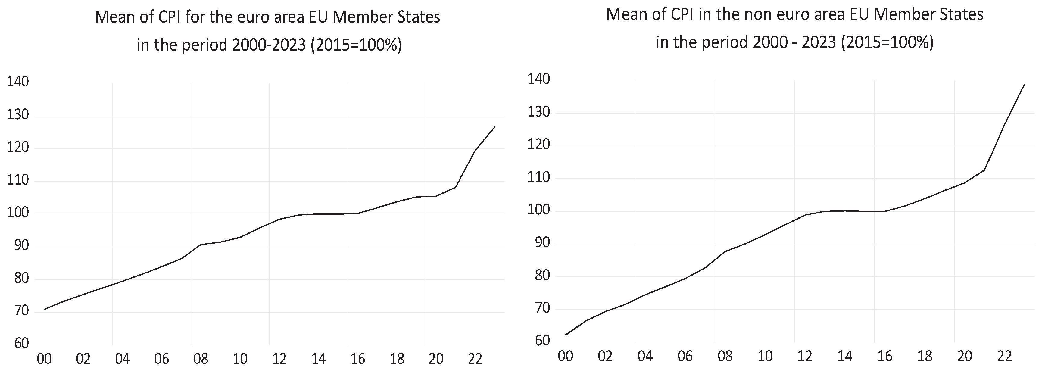
Figure 2.
Average inflation rate and the limit allowed by the price stability criterion in the period 2000-2023.
Figure 2.
Average inflation rate and the limit allowed by the price stability criterion in the period 2000-2023.
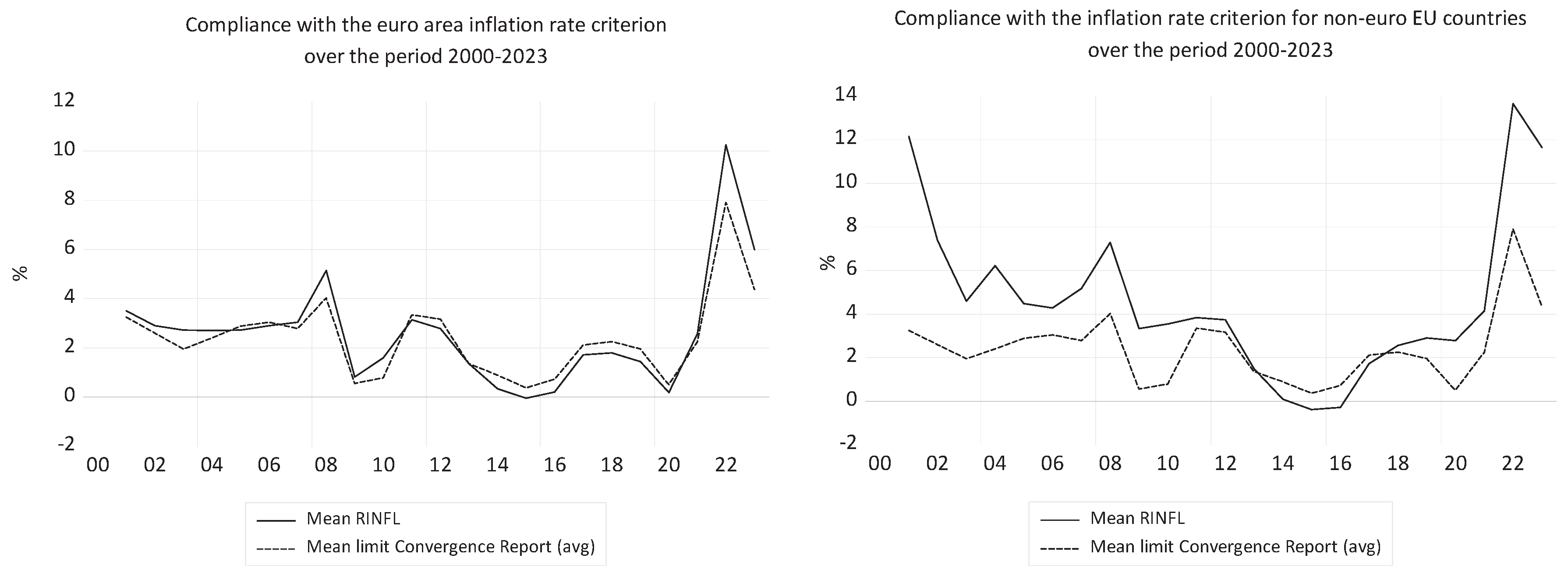
Figure 3.
Compliance with the price stability criterion in the euro area countries.
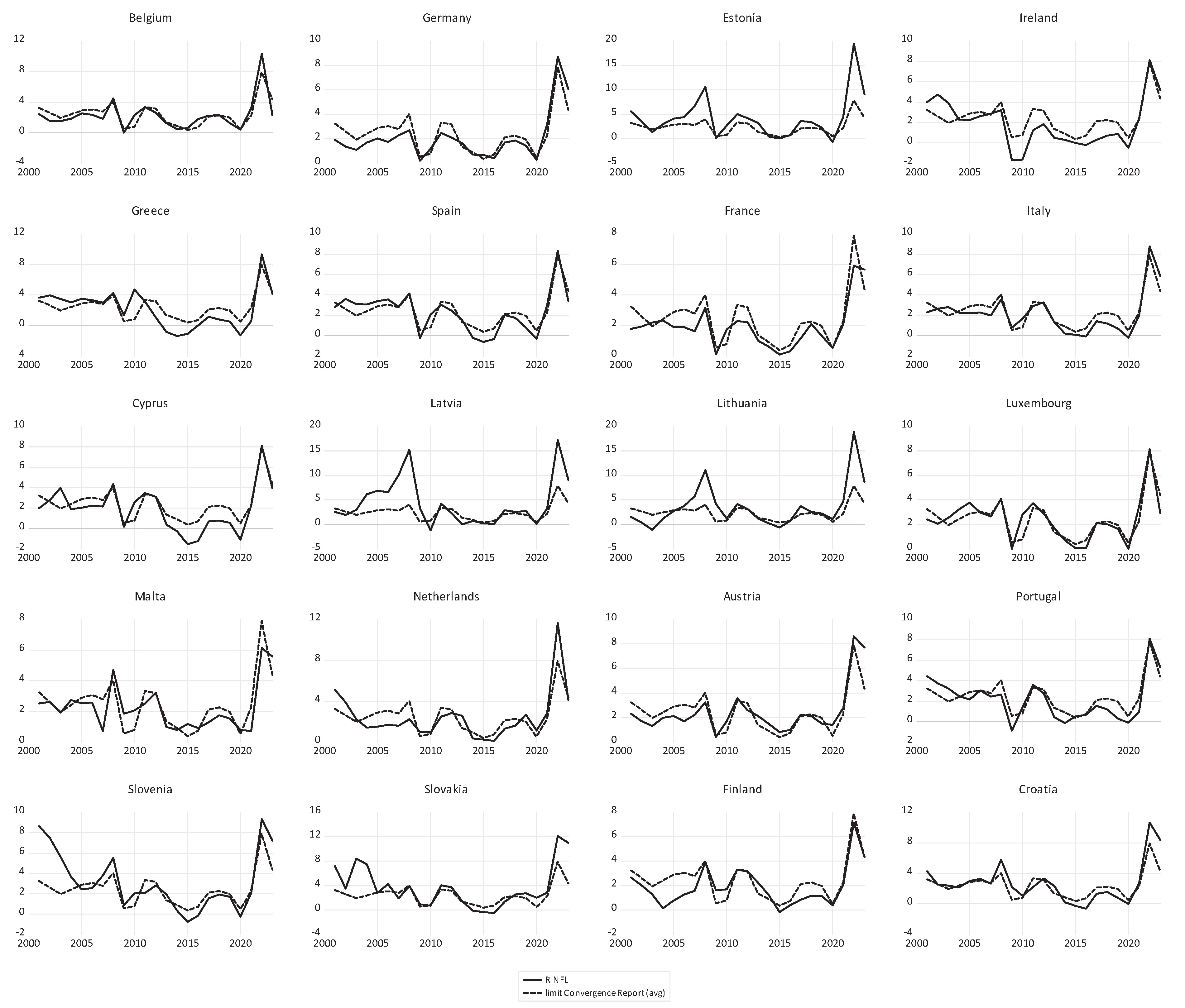
Figure 4.
Compliance with the price stability criterion in EU countries outside the euro area in the period 2000-2023.
Figure 4.
Compliance with the price stability criterion in EU countries outside the euro area in the period 2000-2023.
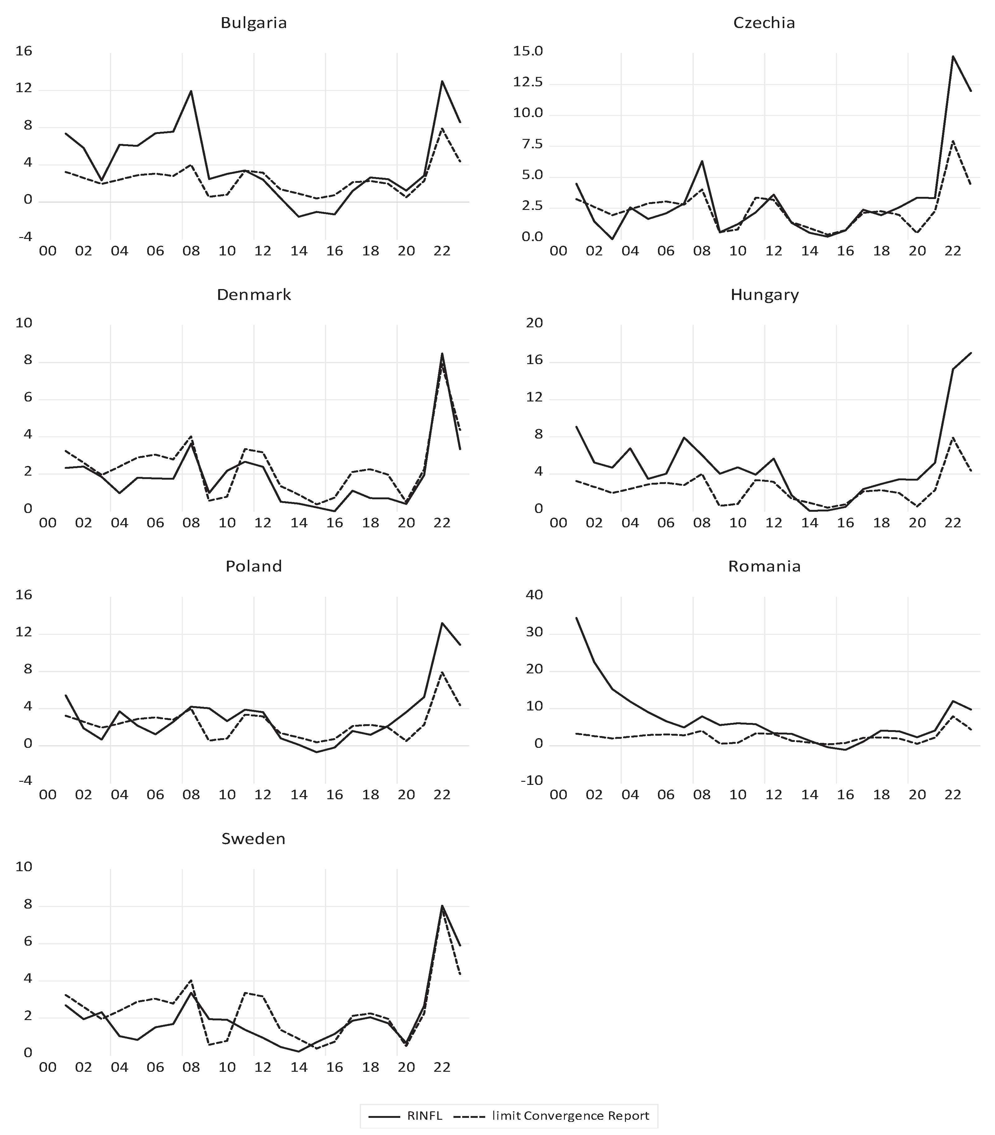
Figure 5.
Compliance with the budget deficit criterion in euro and in EU non-euro countries in the period 2000-2023.
Figure 5.
Compliance with the budget deficit criterion in euro and in EU non-euro countries in the period 2000-2023.
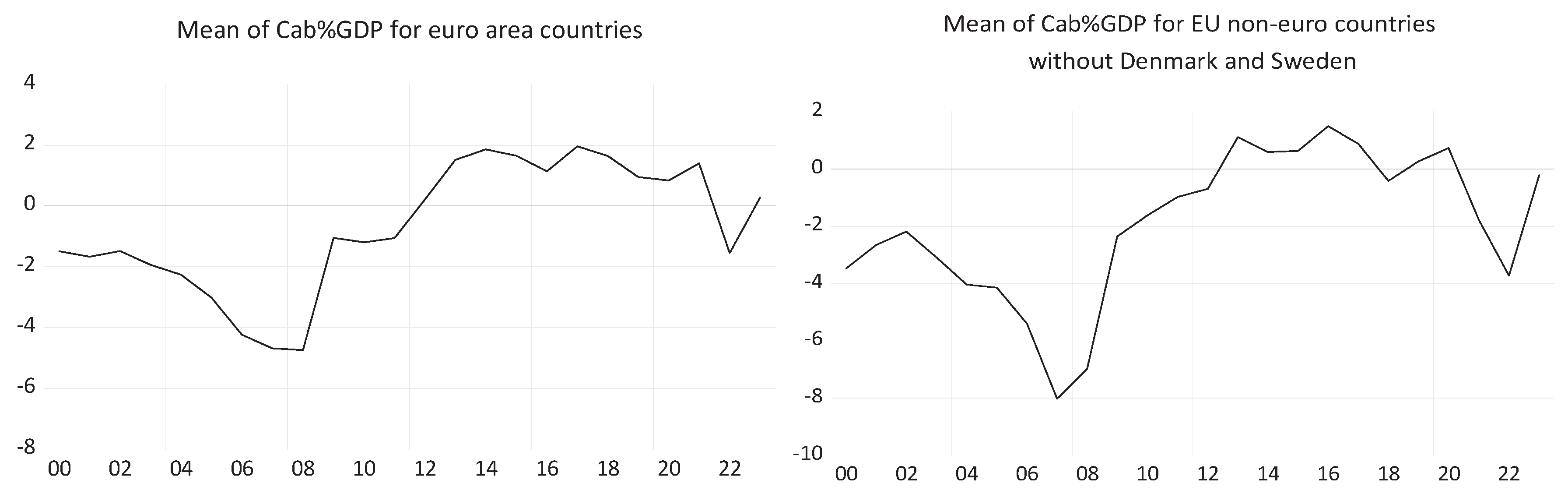
Figure 6.
Compliance with the budgetary criterion in EU non-euro countries.
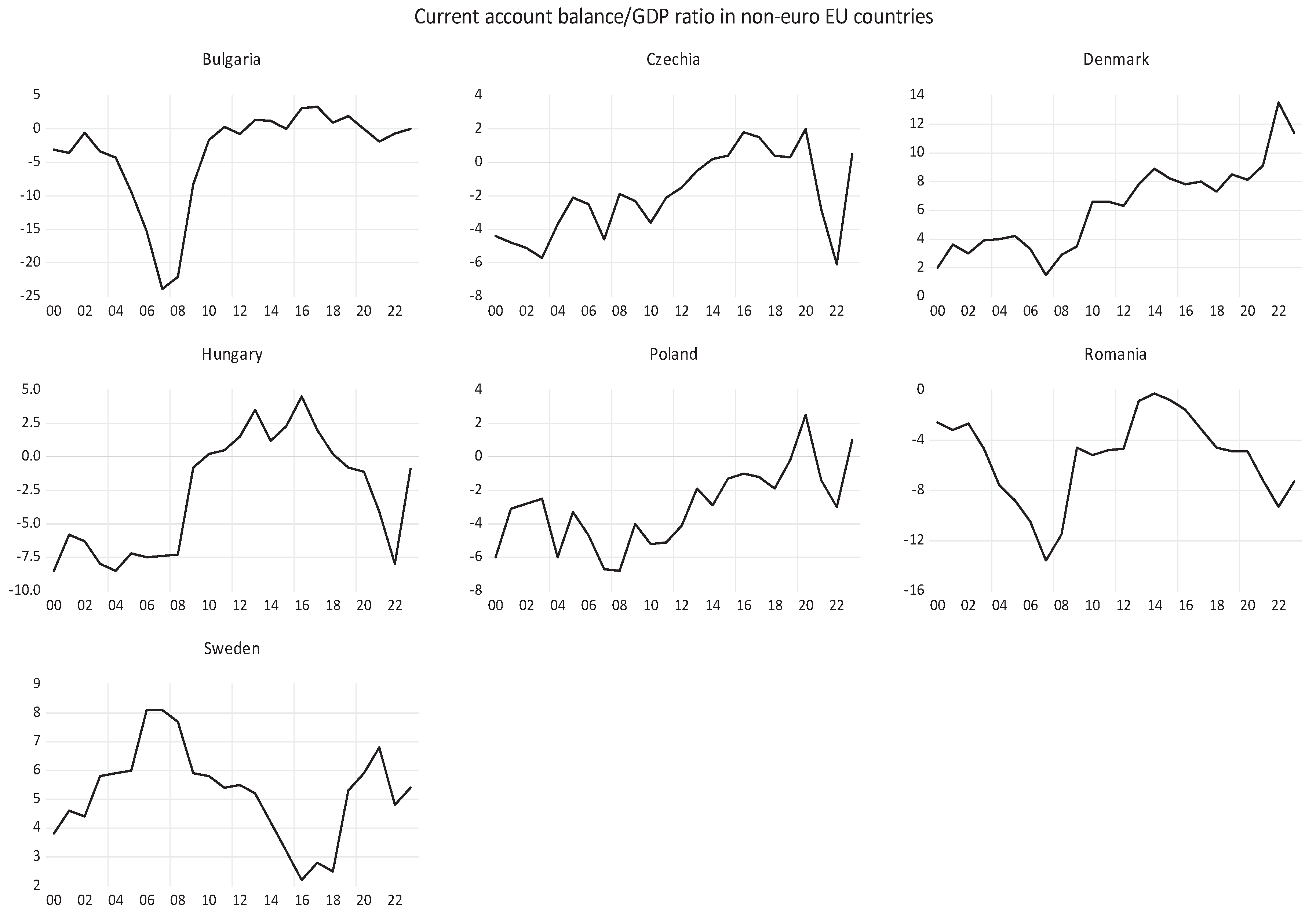
Figure 7.
Compliance with the debt-to-GDP criterion in euro and non-euro area countries.
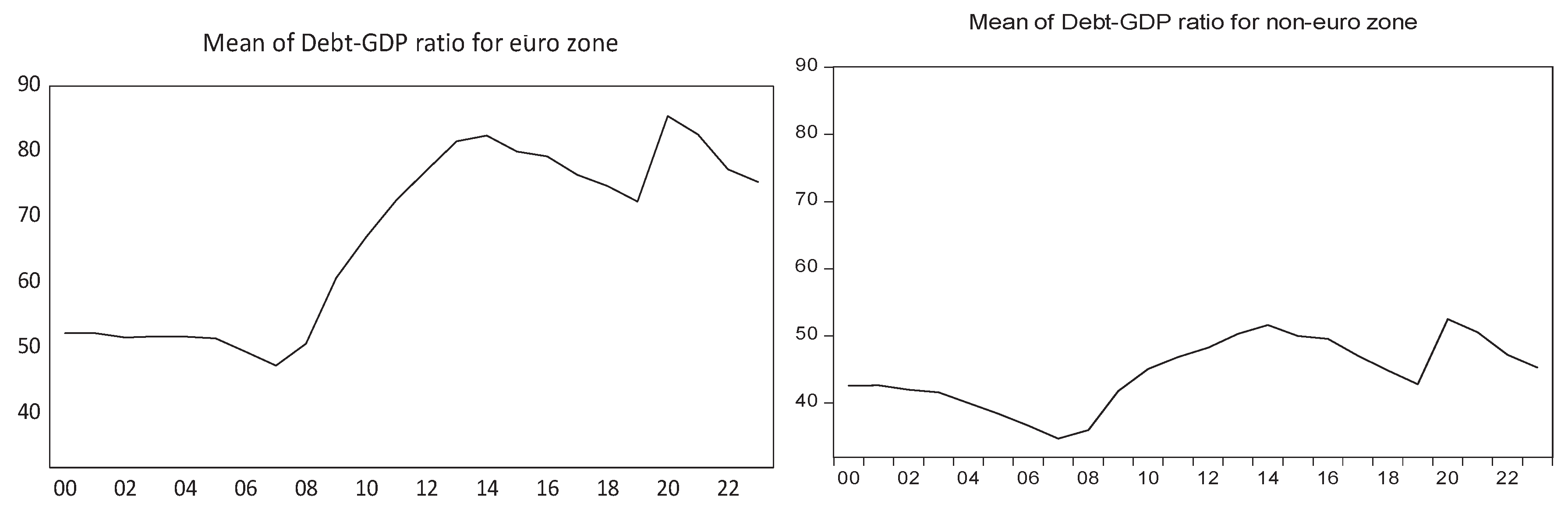
Figure 8.
Compliance with the debt-to-GDP ratio criterion in non-euro EU countries.
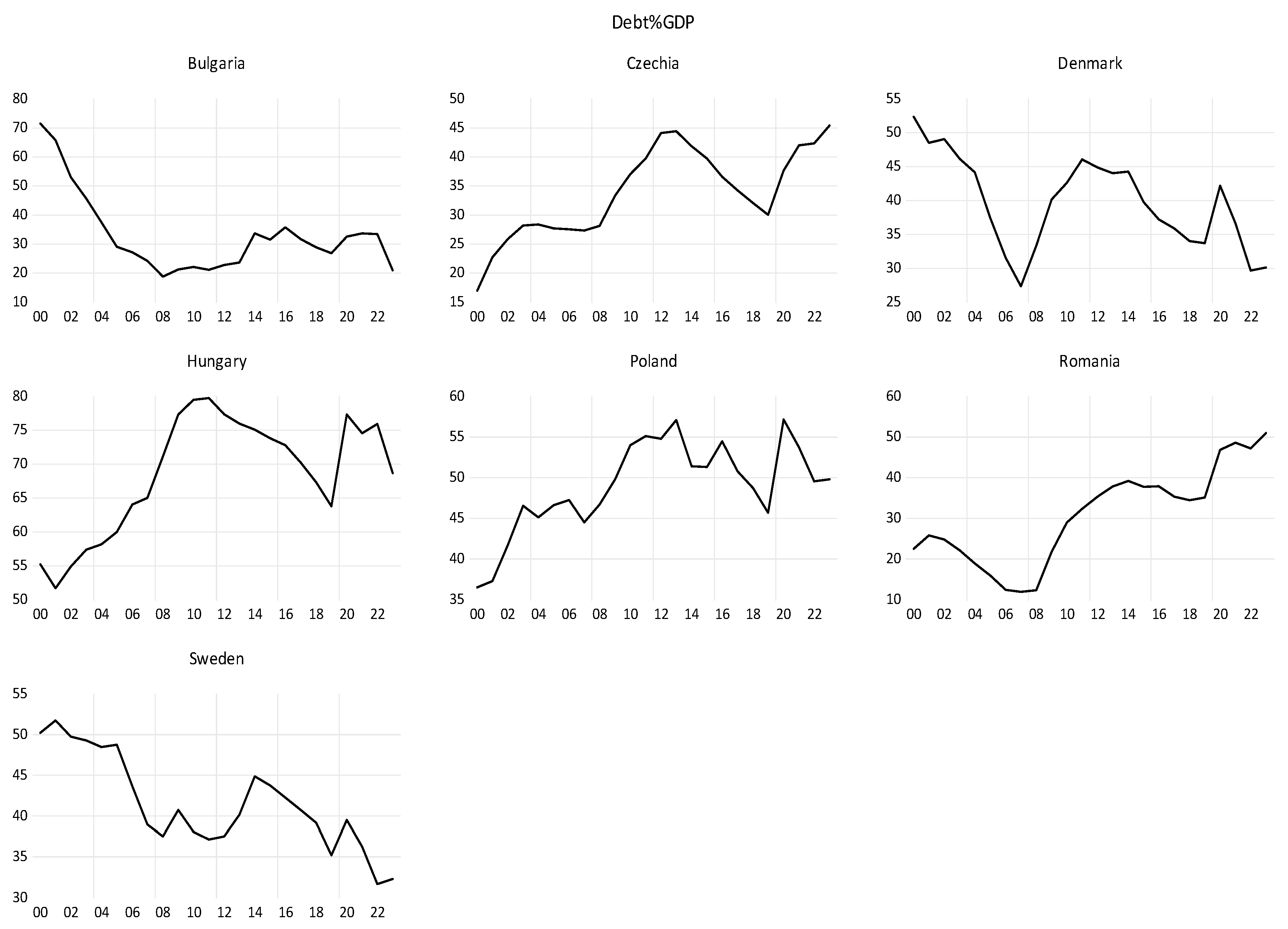
Figure 9.
Compliance with the exchange rate stability criterion both inside and outside the euro area.
Figure 9.
Compliance with the exchange rate stability criterion both inside and outside the euro area.
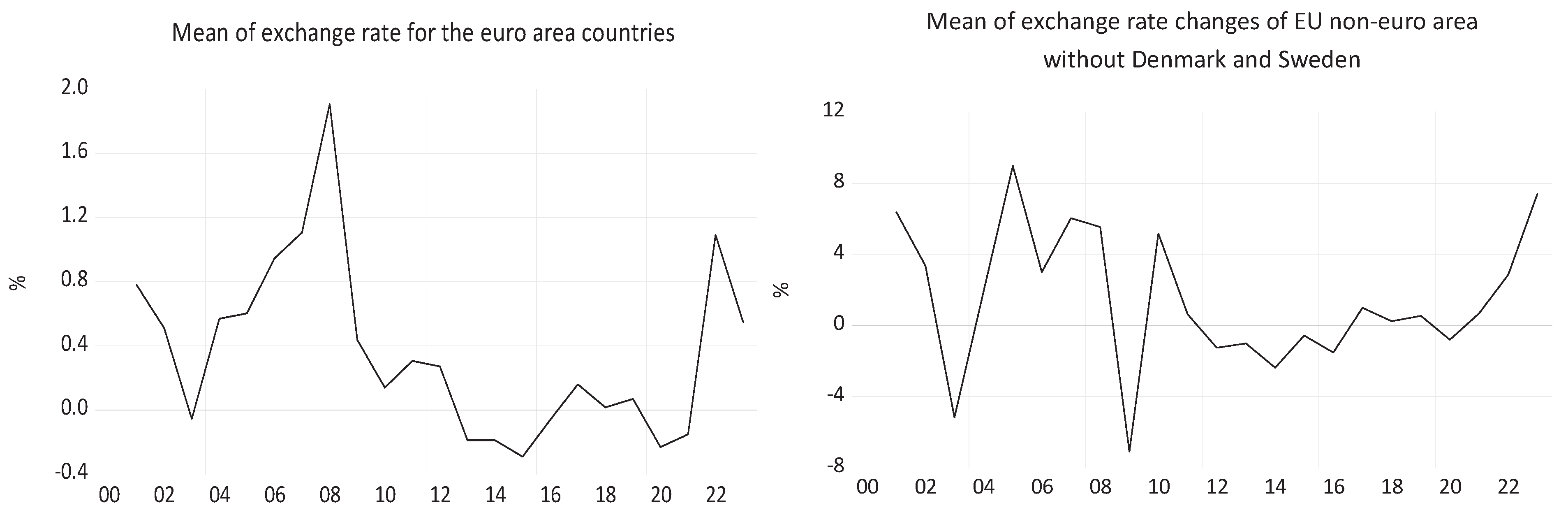
Figure 10.
Compliance with the long-term interest rate criterion both in the euro area and outside the euro area
Figure 10.
Compliance with the long-term interest rate criterion both in the euro area and outside the euro area
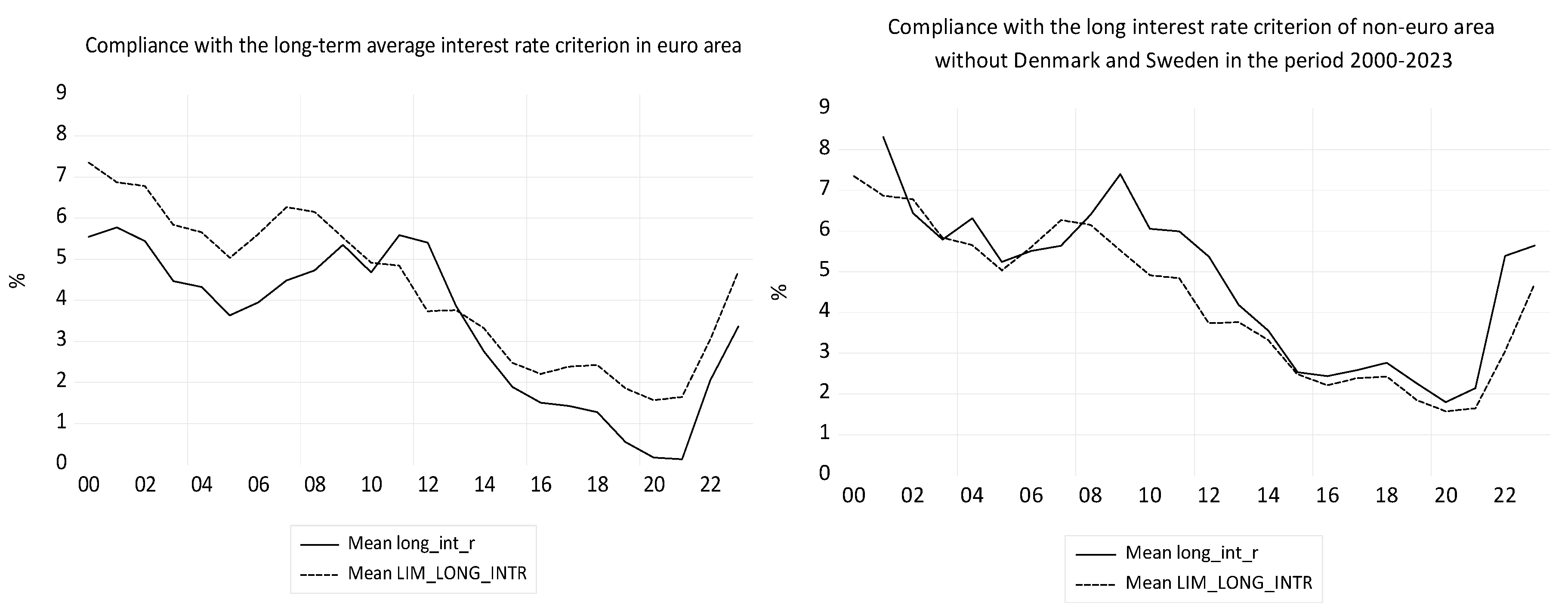
Figure 11.
Compliance with the long-term interest rate criterion in non-euro EU countries
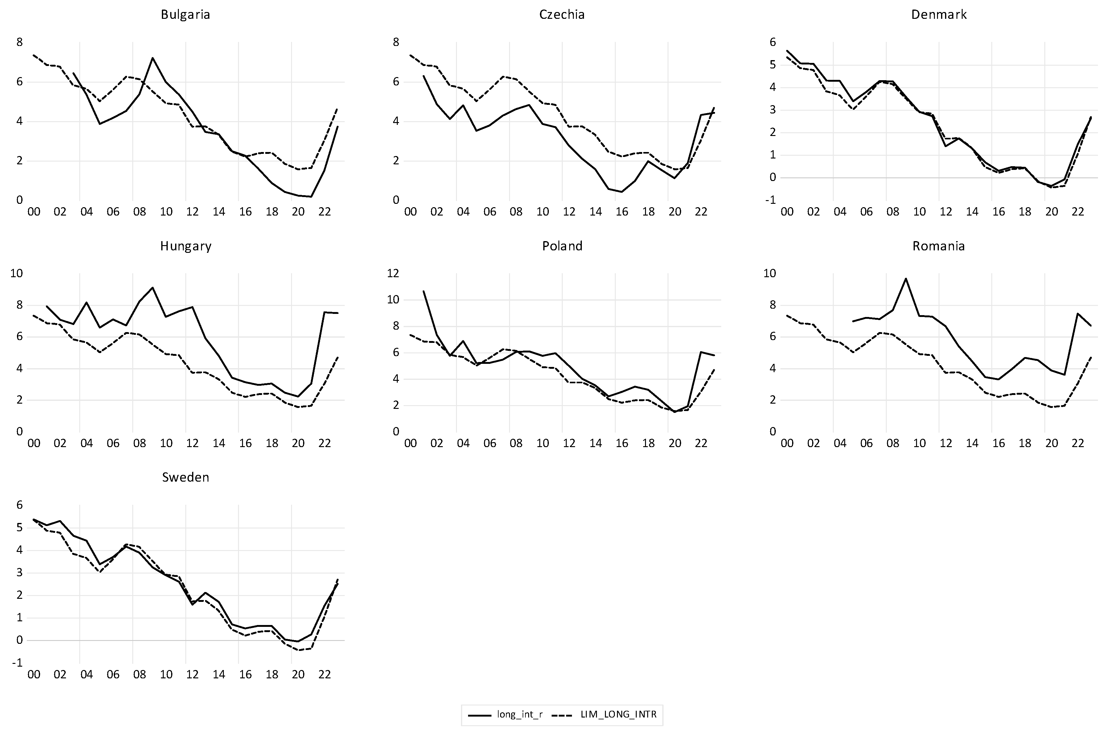
Figure 12.
Average GDP per capita and its average annual changes in the euro area and outside the euro area in the period 2000-2023.
Figure 12.
Average GDP per capita and its average annual changes in the euro area and outside the euro area in the period 2000-2023.
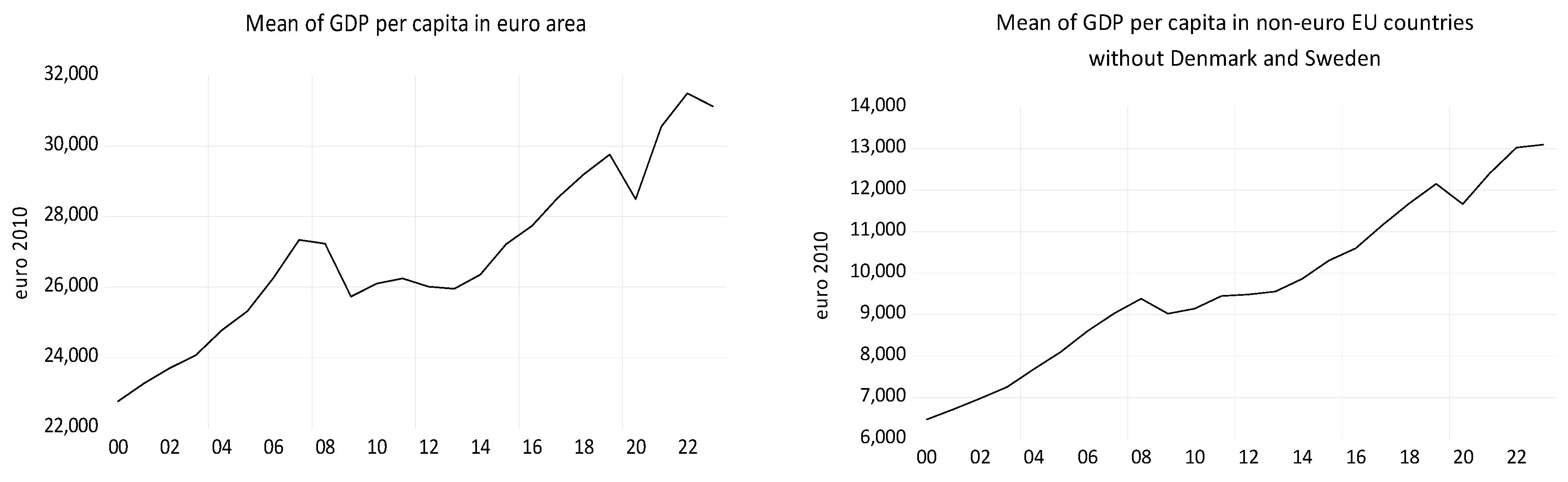
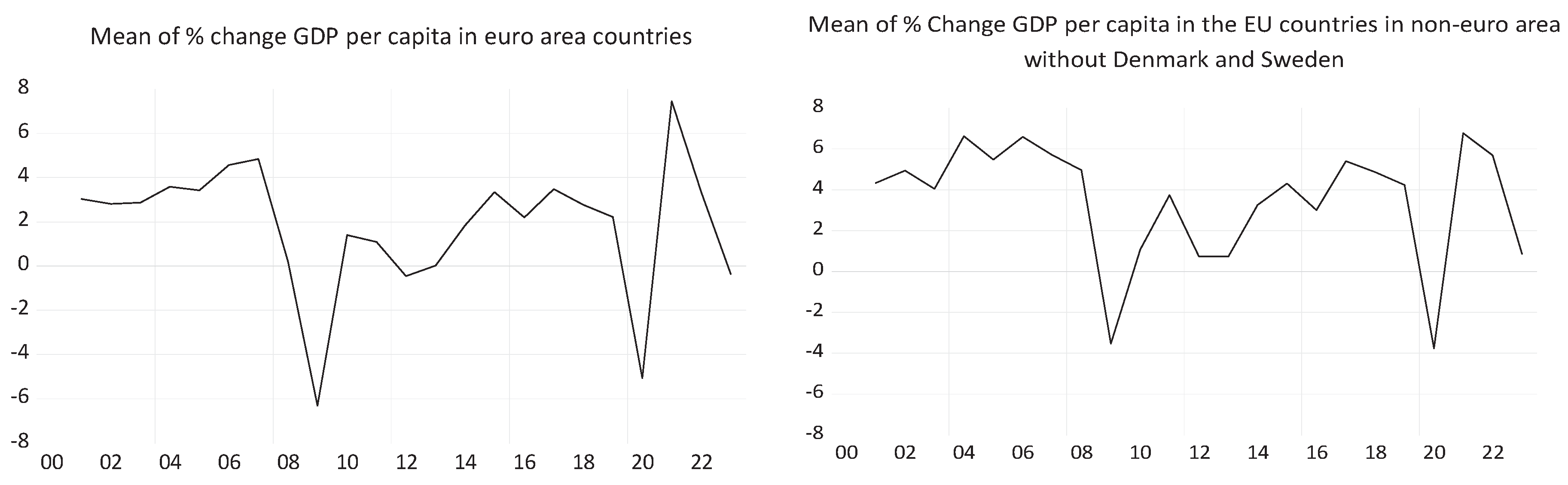
Figure 13.
Evolution of economic convergence indicators in the euro area in the period 2000-2023.
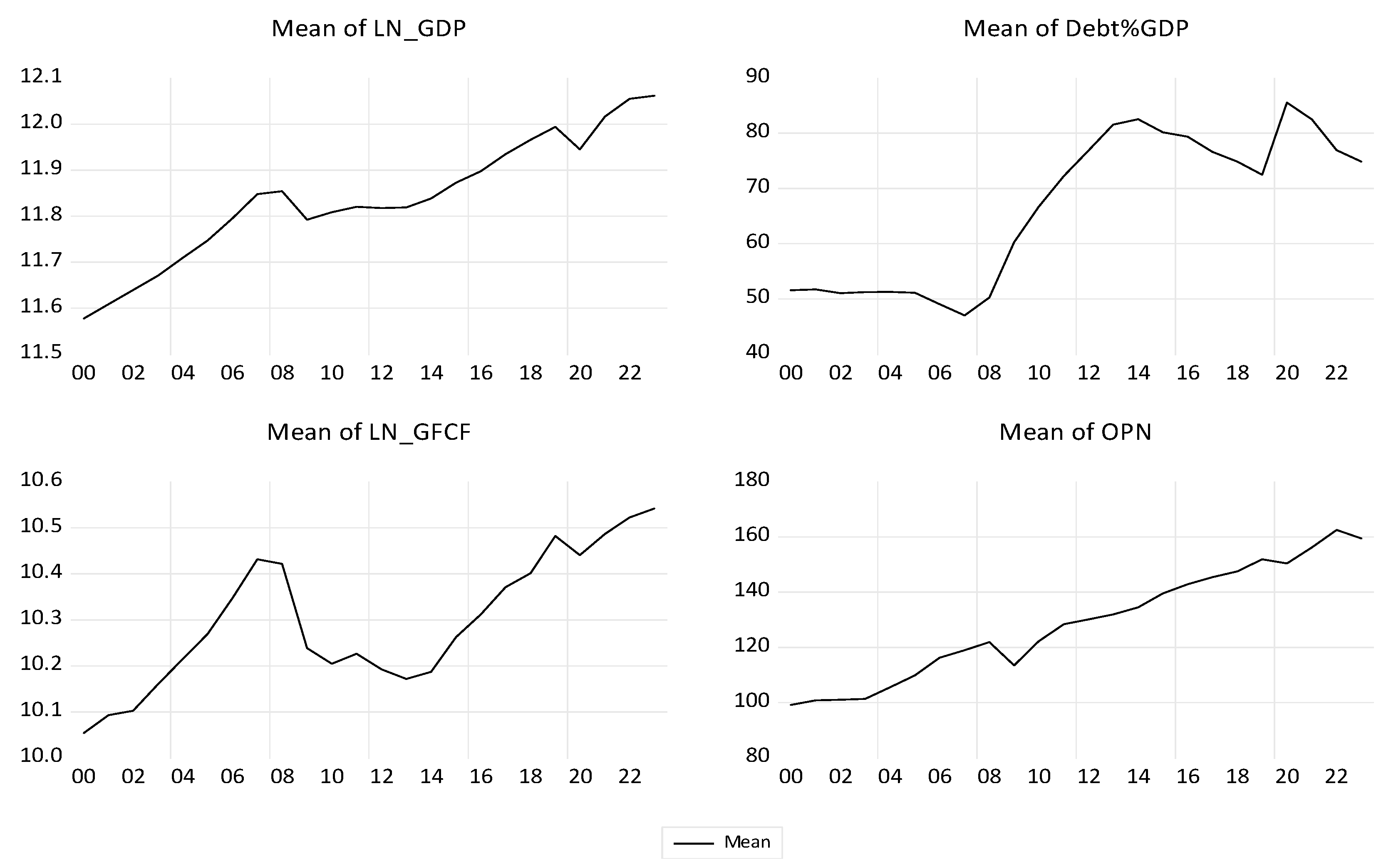
Figure 14.
Adjusting LN_GDP with the ARDL model and with the ECM.
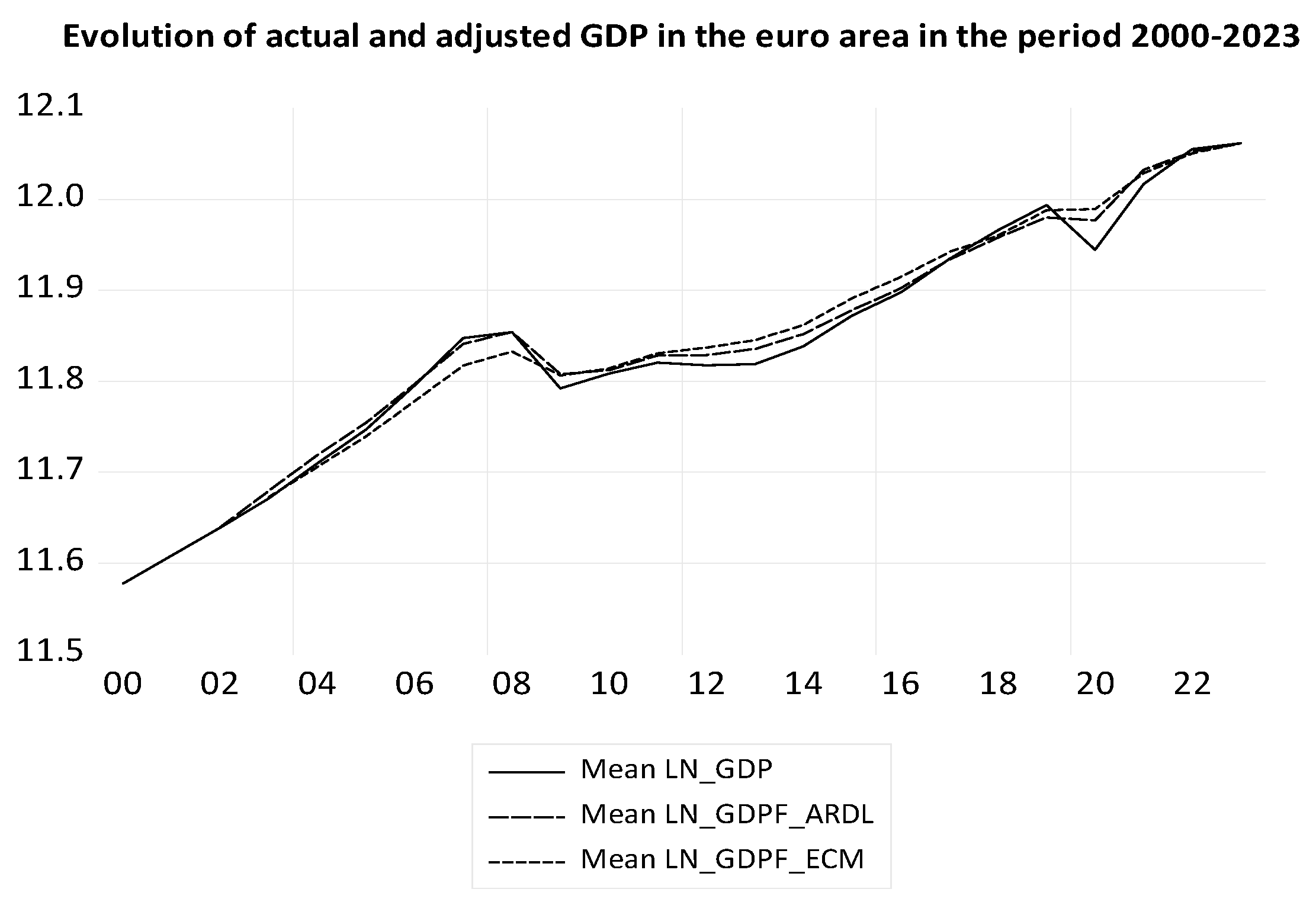
Figure 15.
GDP and its long-term equilibrium in the euro area countries in the period 2000-2023.
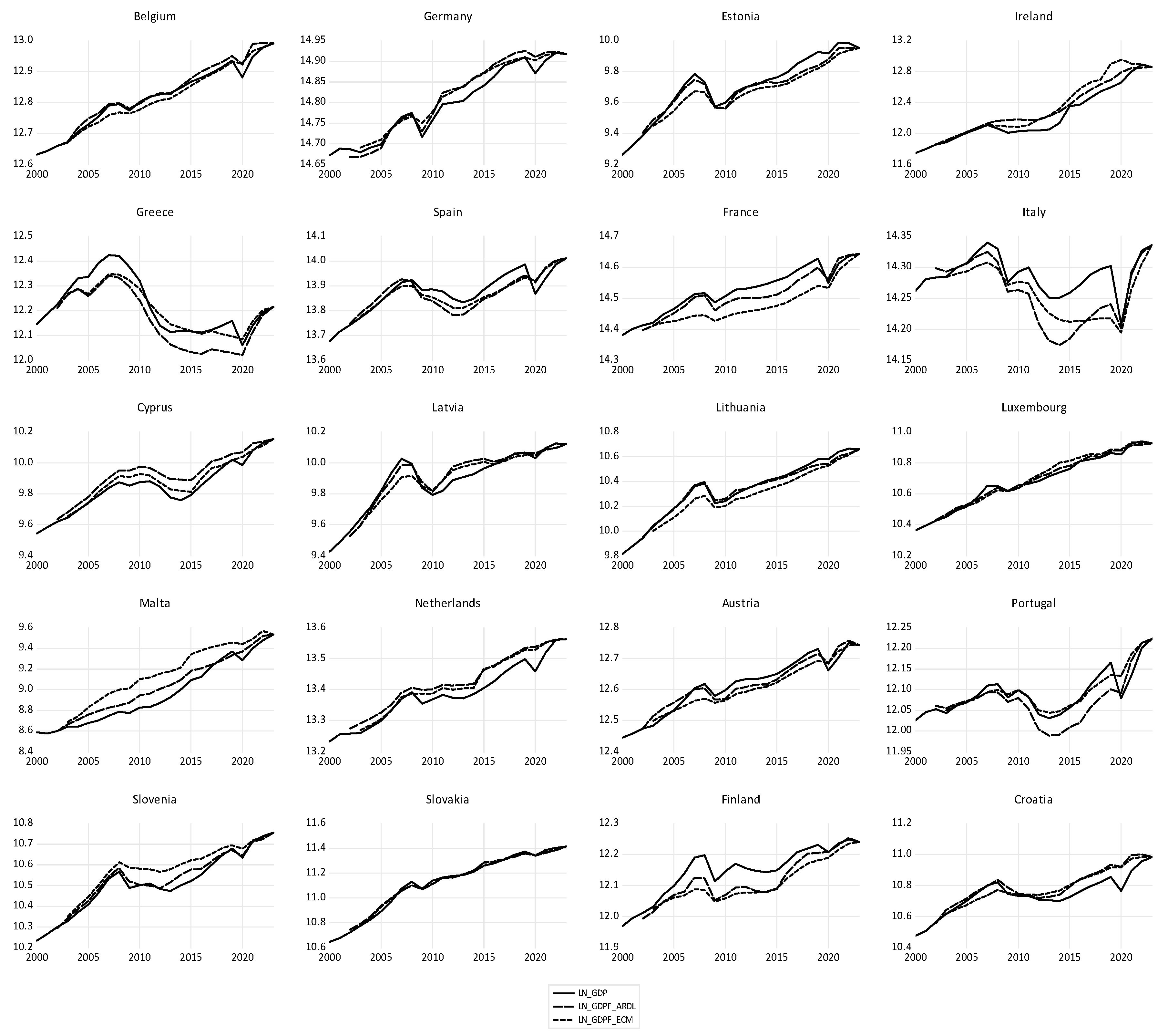
Figure 16.
Economic convergence variables for EU non-euro area countries over the period 2000-2023
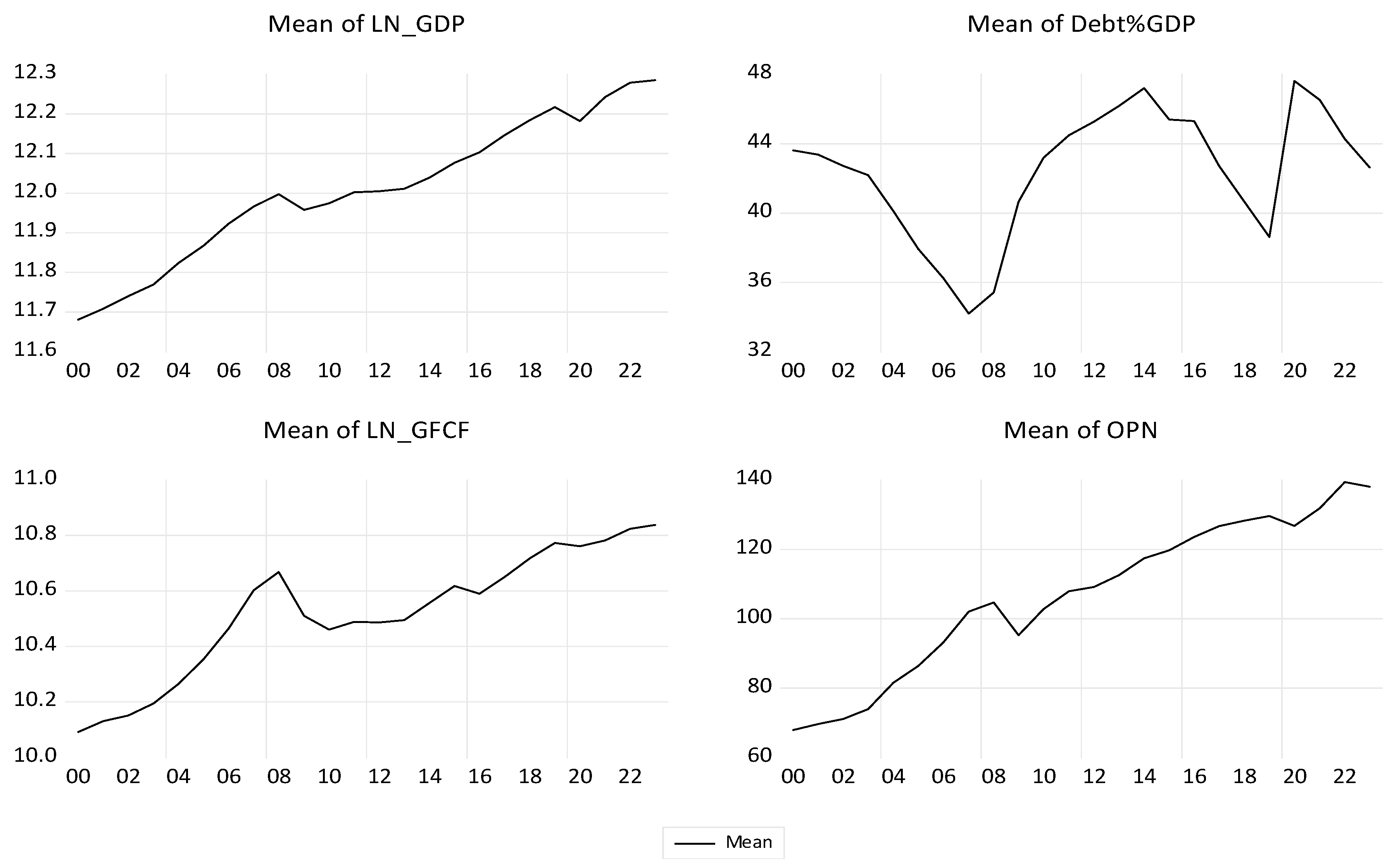
Figure 17.
Economic convergence of GDP growth in non-euro area EU countries over the period 2000-2023 using ECM and ARDL models
Figure 17.
Economic convergence of GDP growth in non-euro area EU countries over the period 2000-2023 using ECM and ARDL models
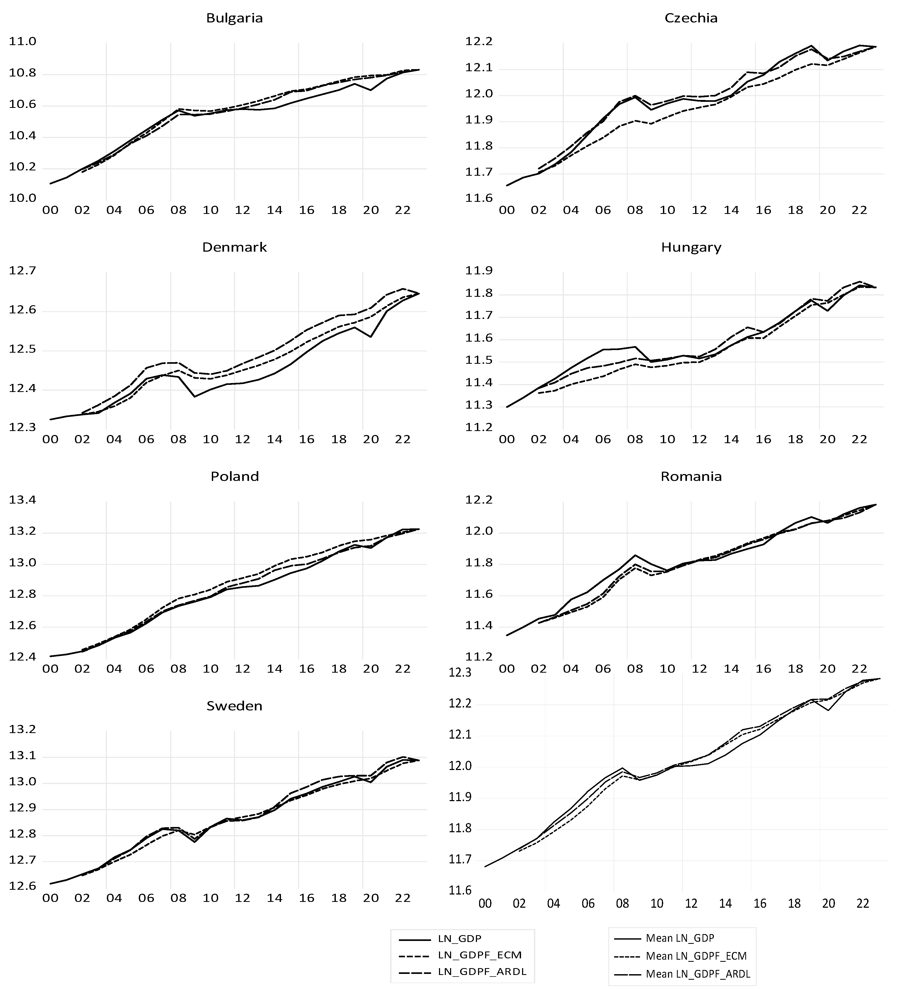
Figure 18.
Economic convergence of GDP growth in the EU during 2000-2023 with ARDL model.
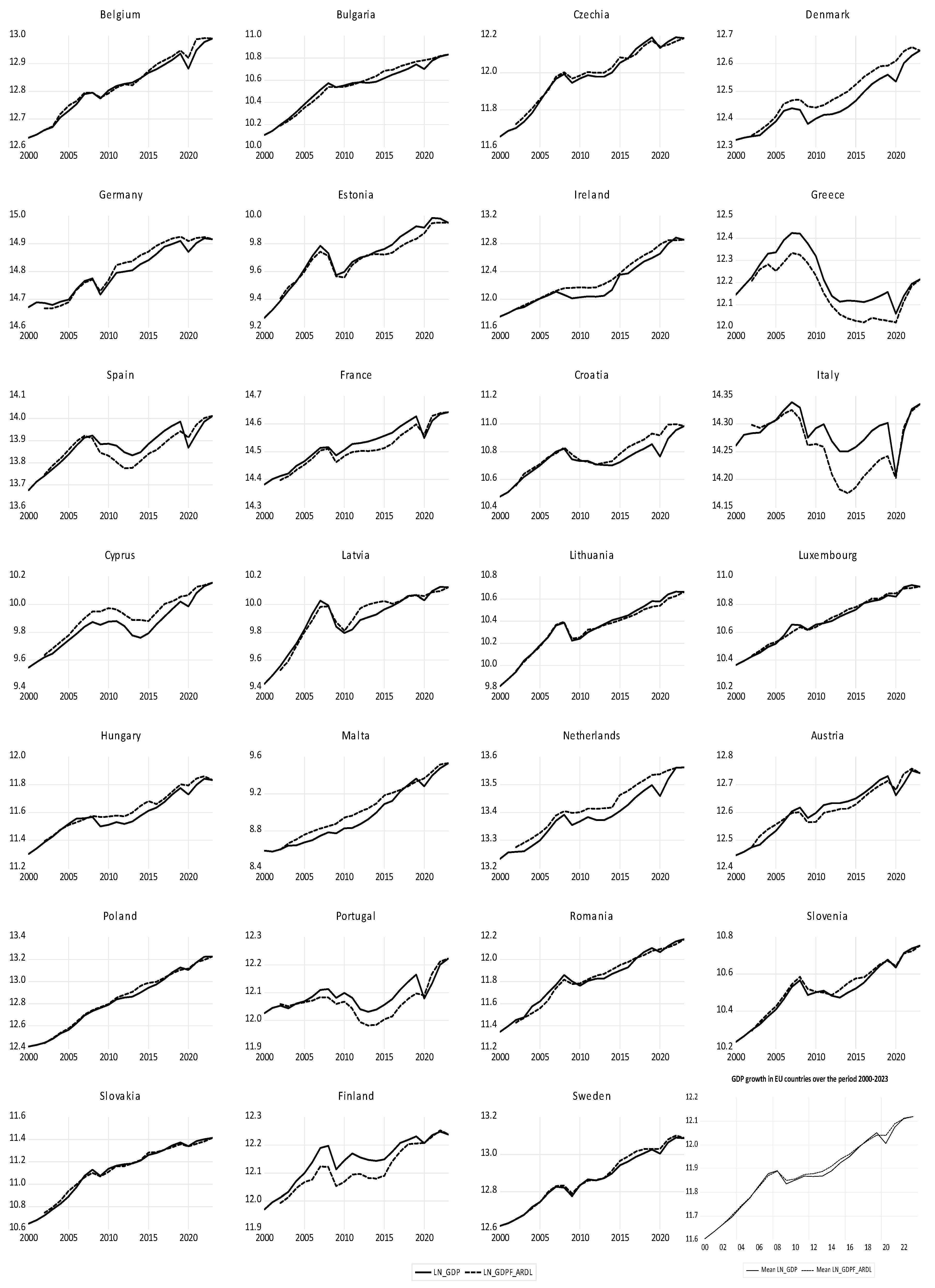
Figure 19.
Evolution of the variables analyzed in the euro area and in the non-euro EU area.
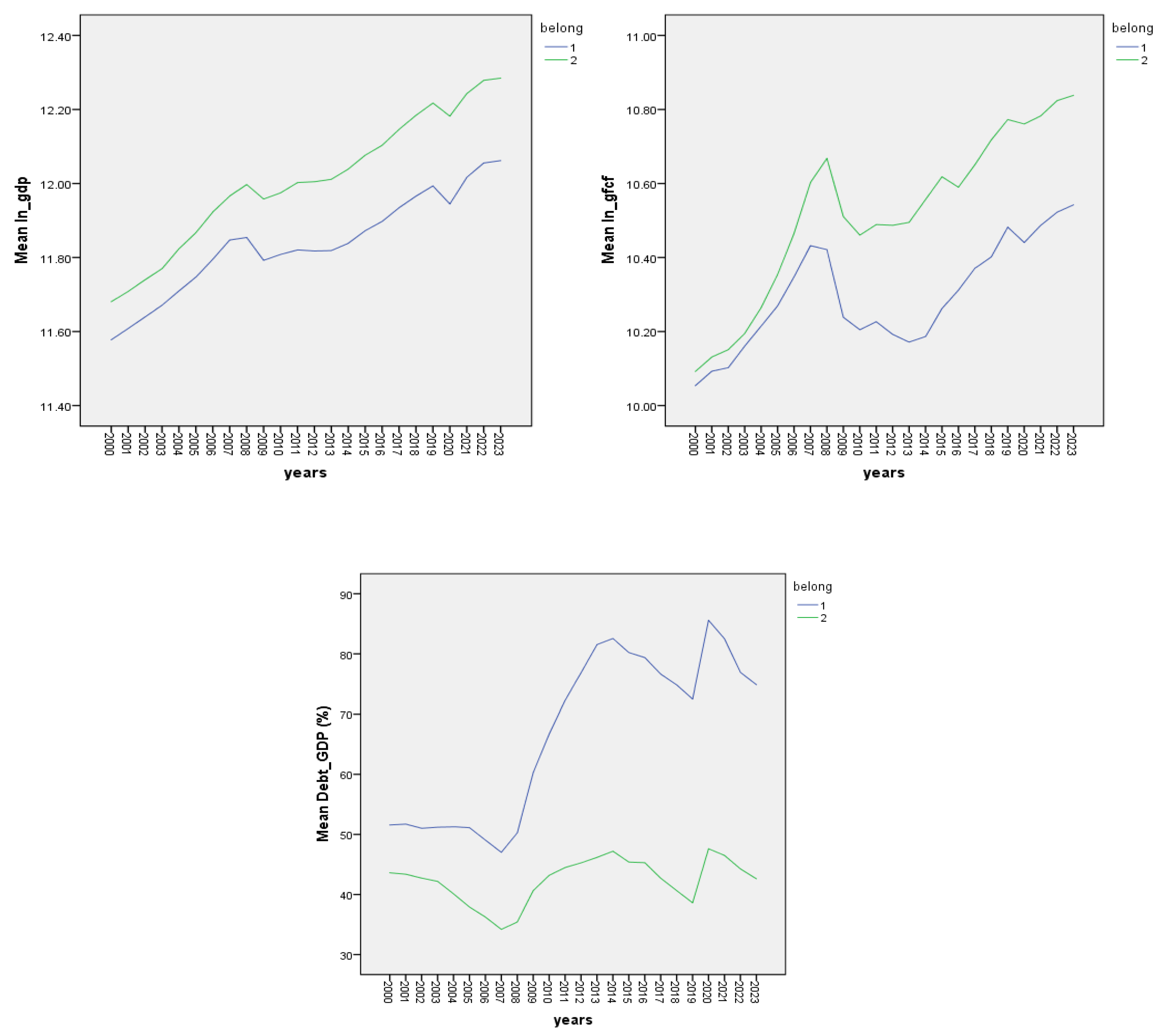
Table 1.
Average annual inflation rate and corresponding average annual limit allowed for the euro area and outside the euro area over the period 2000-2023.
Table 1.
Average annual inflation rate and corresponding average annual limit allowed for the euro area and outside the euro area over the period 2000-2023.
| Euro area | Non-euro | |||
|---|---|---|---|---|
| RINFL (%) | LIM_AVG_INFL (%) | RINFL (%) |
LIM_AVG_INFL (%) | |
| Mean | 1.128651 | 2.406957 | 3.855328 | 2.406957 |
| Median | 0.030261 | 2.250000 | 2.468596 | 2.250000 |
| Maximum | 15.25038 | 7.910000 | 34.45198 | 7.910000 |
| Minimum | -1.086025 | 0.360000 | -1.596573 | 0.360000 |
| Std. Dev. | 1.949242 | 1.622979 | 4.547391 | 1.626272 |
| Skewness | 2.574073 | 1.475974 | 2.976589 | 1.475974 |
| Observations | 460 | 460 | 161 | 161 |
Table 2.
Compliance with the criterion on price stability in the European Union.
| EU groups | Euro area countries | Non-euro area countries | ||||
|---|---|---|---|---|---|---|
| periods | 2000-2008 | 2009-2023 | 2000-2023 | 2000-2008 | 2009-2023 | 2000-2023 |
| r | 0.321 | 0.857 | 0.783 | 0.146 | 0.800 | 0.566 |
| conformity | weak | strong | strong | lack | strong | medium |
Table 3.
Statistical summary of the budget deficit and debt-to-GDP ratio in euro area and non-euro area EU countries over the period 2000-2023
Table 3.
Statistical summary of the budget deficit and debt-to-GDP ratio in euro area and non-euro area EU countries over the period 2000-2023
| Euro area | Non-euro | |||
|---|---|---|---|---|
| CAB_GDP (%) | DEBT_GDP (%) | CAB_GDP (%) | DEBT_GDP (%) | |
| Mean | -0.703958 | 66.57701 | -0.748214 | 42.34829 |
| Median | -0.200000 | 63.62830 | -0.800000 | 40.17136 |
| Maximum | 13.70000 | 212.3881 | 13.50000 | 79.77408 |
| Minimum | -20.80000 | 3.764939 | -23.90000 | 11.94916 |
| Std. Dev. | 5.467112 | 38.53018 | 5.734244 | 15.09071 |
| Skewness | -0.492769 | 0.781217 | -0.588121 | 0.562073 |
| Kurtosis | 3.564701 | 3.787907 | 4.596349 | 3.046301 |
| Jarque-Bera | 25.80344 | 61.23995 | 27.52311 | 8.860938 |
| Probability | 0.000002 | 0.000000 | 0.000001 | 0.011909 |
| Observations | 480 | 480 | 168 | 168 |
Table 4.
Statistical summary of the dynamic rhythms of exchange rates in the euro area and in the non-euro area over the period 2000-2023.
Table 4.
Statistical summary of the dynamic rhythms of exchange rates in the euro area and in the non-euro area over the period 2000-2023.
| Euro area | Non-euro | Non-euro without Denmark and Sweden | |
|---|---|---|---|
| REXCH (%) | REXCH (%) | REXCH (%) | |
| Mean | 0.360484 | 0.807164 | 1.471498 |
| Median | 0.124715 | -0.001766 | 0.626149 |
| Maximum | 9.943644 | 19.45867 | 19.45867 |
| Minimum | -8.213416 | -16.00922 | -16.00922 |
| Std. Dev. | 1.776734 | 4.877708 | 5.260163 |
| Skewness | 2.036987 | 0.461658 | 0.235303 |
| Kurtosis | 13.01488 | 5.111733 | 4.649911 |
| Jarque-Bera | 2240.488 | 35.63420 | 14.10511 |
| Probability | 0.000000 | 0.000000 | 0.000865 |
| Observations | 460 | 161 | 115 |
Table 5.
Independent samples t-test for euro area and non-euro area (REXCH).
| Levene's Test for Equality of Variances |
t-test for Equality of Means | ||||||||
|---|---|---|---|---|---|---|---|---|---|
| F | Sig. | t | df | Sig. (2-tailed) | Mean Difference | Std. Error Difference | 95% Confidence Interval of the Difference | ||
| Lower | Upper | ||||||||
| Equal variances assumed |
139.921 | 0.000 | -1.674 | 619 | 0.095 | -0.447 | 0.267 | -0.971 | 0.077 |
| Equal variances not assumed |
-1.136 | 175.074 | 0.258 | -0.447 | 0.393 | -1.223 | 0.329 | ||
Table 6.
Testing REXCH for euro area and non-euro area without Denmark and Sweden
| Levene's Test for Equality of Variances | t-test for Equality of Means | ||||||||
|---|---|---|---|---|---|---|---|---|---|
| F | Sig. | t | df | Sig. (2-tailed) | Mean Difference | Std. Error Difference | 95% Confidence Interval of the Difference | ||
| Lower | Upper | ||||||||
| Equal variances assumed |
169.148 | 0.000 | -3.760 | 573 | 0.000 | -1.111 | 0.295 | -1.691 | -0.531 |
| Equal variances not assumed |
-2.233 | 120.57 | 0.027 | -1.111 | 0.497 | -2.096 | -0.126 | ||
Table 7.
One-sample t tests and 95% confidence intervals of REXCH in the period 2000-2023
| Variable REXCH | N | Mean | Std. Deviation | Std. Error Mean | t | df | Sig. (2-tailed) | 95% confidence interval | |
|---|---|---|---|---|---|---|---|---|---|
| Lower | Upper | ||||||||
| Euro area | 460 | 0.360 | 1.777 | 0.083 | 4.352 | 459 | 0.000 | 0.1977 | 0.5233 |
| Non-euro area | 161 | 0.807 | 4.878 | 0.384 | 2.100 | 160 | 0.037 | 0.0480 | 1.5665 |
| Non-euro, no DK, SW | 115 | 1.471 | 5.260 | 0.490 | 3.000 | 114 | 0.003 | 0.4998 | 2.4432 |
| EU | 621 | 0.476 | 2.918 | 0.117 | 4.067 | 620 | 0.000 | 0.2463 | 0.7062 |
Table 8.
Average long-term interest rate and corresponding permitted limit, for both the euro area and non-euro area countries, over the period 2000-2023.
Table 8.
Average long-term interest rate and corresponding permitted limit, for both the euro area and non-euro area countries, over the period 2000-2023.
| Euro area | Non-euro | Non-euro, no Denmark and Sweden | ||||
|---|---|---|---|---|---|---|
| long_int_r (%) | limit_long_intr (%) | long_int_r (%) | limit_long_intr (%) | long_int_r (%) | limit_long_intr (%) | |
| Mean | 3.362 | 4.246 | 3.998 | 3.541 | 4.654 | 4.074 |
| Median | 3.650 | 4.697 | 3.890 | 3.610 | 4.540 | 3.760 |
| Maximum | 22.500 | 7.350 | 10.680 | 6.867 | 10.680 | 6.867 |
| Minimum | -0.510 | 1.567 | -0.360 | -0.433 | 0.190 | 1.567 |
| Std. Dev. | 2.477 | 1.758 | 2.364 | 1.888 | 2.283 | 1.670 |
| Skewness | 1.703 | -0.032 | 0.190 | -0.160 | 0.072 | -0.018 |
| Kurtosis | 12.258 | 1.669 | 2.433 | 2.129 | 2.401 | 1.614 |
| Jarque-Bera | 1816.664 | 33.154 | 3.052 | 5.627 | 1.725 | 8.731 |
| Probability | 0.000 | 0.000 | 0.217 | 0.060 | 0.422 | 0.013 |
| Observations | 448 | 448 | 157 | 157 | 109 | 109 |
Table 9.
Summarizing the conformity with long-term interest rate criterion in EU.
| EU groups | periods | conformity | ||||
|---|---|---|---|---|---|---|
| 2000-2008 | 2009-2023 | 2000-2023 | 2000-2008 | 2009-2023 | 2000-2023 | |
| Euro area | 0.680 | 0.627 | 0.661 | medium | medium | medium |
| Non-euro area | 0.638 | 0.826 | 0.828 | medium | strong | strong |
| Non-euro no DK, SW | 0.383 | 0.739 | 0.726 | weak | medium | medium |
Table 10.
Correlations of variables of euro area in the period 2000-2023.
| LN_GDP | DEBT_GDP | LN_GFCF | OPN | |
|---|---|---|---|---|
| LN_GDP | 1 | |||
| DEBT_GDP | 0.4768 | 1 | ||
| LN_GFCF | 0.9946 | 0.4212 | 1 | |
| OPN | -0.5040 | -0.3828 | -0.5006 | 1 |
Table 11.
Granger causality analysis for the euro area by sub-periods and for the period 2000-2023
| Variable Granger cause | for variable | 2000 - 2008 | 2009-2023 | 2000-2023 |
|---|---|---|---|---|
| No. obs. | 180 | 300 | 480 | |
| LN_GDP | DEBT_GDP | - | - | √ |
| LN_GFCF | √ | √ | √ | |
| OPN | - | - | √ | |
| DEBT_GDP | LN_GDP | - | - | - |
| LN_GFCF | - | √ | √ | |
| OPN | - | - | - | |
| LN_GFCF | LN_GDP | - | - | - |
| DEBT_GDP | - | - | √ | |
| OPN | - | √ | √ | |
| OPN | LN_GDP | √ | √ | - |
| DEBT_GDP | - | √ | √ | |
| LN_GFCF | - | - | - | |
Table 12.
Comparison of ECM and ARDL models for the euro area over the period 2000-2023.
| LN_GDP – dependent variable | Error Correction Model | ARDL | ||
|---|---|---|---|---|
| Long-run | Short-run FE cross-sections (SUR) | Long-run | Short-run | |
| C | - | 0.0128*** | - | 1.1172*** |
| DEBT_GDP(-1) | 0.0031*** | 0.0009*** | 0.0029*** | 0.0002 |
| LN_GFCF | 0.6629*** | 0.2463*** | 0.5795*** | 0.2196*** |
| ECT(-1) | - | -0.1870*** | - | -0.1972*** |
(*/ **/ *** significance p-value less than: 10%/ 5%/ 1%).
Table 13.
The short-run coefficients for each euro area country over the period 2000-2023
| Number | Country | COINTEQ01 | D(DEBT_GDP(-1)) | D(LN_GFCF) | C |
|---|---|---|---|---|---|
| 1 | Portugal | -0.402*** | 0.000*** | 0.097*** | 2.310** |
| 2 | Belgium | -0.395*** | 0.001*** | 0.239*** | 2.354*** |
| 3 | Croatia | -0.362*** | 0.000*** | 0.206*** | 1.904 |
| 4 | Lithuania | -0.349*** | 0.001*** | 0.142*** | 1.826*** |
| 5 | Austria | -0.327*** | 0.001*** | 0.296*** | 1.945** |
| 6 | Greece | -0.294*** | 0.000*** | 0.127*** | 1.710** |
| 7 | Cyprus | -0.280*** | 0.001*** | 0.038*** | 1.376*** |
| 8 | Latvia | -0.243*** | -0.001*** | 0.177*** | 1.215*** |
| 9 | Estonia | -0.201*** | 0.003*** | 0.233*** | 0.971** |
| 10 | Spain | -0.194*** | 0.001*** | 0.269*** | 1.266 |
| 11 | Netherlands | -0.179*** | -0.001*** | 0.064*** | 1.151 |
| 12 | Finland | -0.167*** | 0.000*** | 0.401*** | 0.977** |
| 13 | Ireland | -0.145*** | -0.002*** | -0.071*** | 0.882** |
| 14 | Germany | -0.140*** | 0.001*** | 0.416*** | 0.980* |
| 15 | Slovakia | -0.139*** | 0.000*** | 0.176*** | 0.777*** |
| 16 | Luxembourg | -0.115*** | -0.004*** | 0.108*** | 0.649** |
| 17 | Slovenia | -0.109*** | 0.001*** | 0.288*** | 0.577*** |
| 18 | France | 0.004 | 0.001*** | 0.554*** | -0.028 |
| 19 | Malta | 0.039*** | 0.001*** | 0.126*** | -0.139 |
| 20 | Italy | 0.054** | 0.000*** | 0.505*** | -0.357 |
| Euro area | -0.1972*** | 0.0002 | 0.2196*** | 1.1172*** |
(*/ **/ *** significance p-value less than: 10%/ 5%/ 1%).
Table 14.
Correlations of variables for non-euro area over the period 2000-2023
| LN_GDP | DEBT_GDP | LN_GFCF | OPN | |
|---|---|---|---|---|
| LN_GDP | 1 | |||
| DEBT_GDP | 0.1198 | 1 | ||
| LN_GFCF | 0.9813 | 0.0655 | 1 | |
| OPN | -0.2076 | 0.4388 | -0.1576 | 1 |
Table 15.
Granger causality analysis for the non-euro area by sub-periods and for the period 2000-2023
Table 15.
Granger causality analysis for the non-euro area by sub-periods and for the period 2000-2023
| Variable Granger cause | for variable: | Non-euro area | Non-euro area without Denmark and Sweden | ||||
|---|---|---|---|---|---|---|---|
| 2000 - 2008 | 2009 -2023 | 2000 -2023 | 2000 - 2008 | 2009 -2023 | 2000 -2023 | ||
| No. obs. | 63 | 105 | 168 | 45 | 75 | 120 | |
| LN_GDP | DEBT_GDP | - | - | - | √ | - | √ |
| LN_GFCF | √ | √ | √ | - | √ | √ | |
| OPN | - | - | √ | - | √ | √ | |
| DEBT_GDP | LN_GDP | - | - | - | √ | - | - |
| LN_GFCF | - | √ | - | - | √ | - | |
| OPN | - | - | - | √ | - | ||
| LN_GFCF | LN_GDP | - | - | √ | √ | √ | √ |
| DEBT_GDP | - | - | - | √ | - | √ | |
| OPN | - | √ | √ | - | √ | √ | |
| OPN | LN_GDP | √ | - | √ | - | - | √ |
| DEBT_GDP | - | - | - | - | - | - | |
| LN_GFCF | - | √ | √ | - | √ | √ | |
Table 16.
Comparing the ECM and ARDL models for non-euro EU area in the period 2000-2023.
| LN_GDP – dependent variable | Error Correction Model | ARDL(1,1,1) | ||
| Long-run | Short-run FE cross-section (SUR) | Long-run | Short-run | |
| C | - | 0.0179*** | - | 0.8547*** |
| DEBT_GDP(-1) | 0.0030*** | 0.0007** | 0.0049*** | 0.0007 |
| LN_GFCF | 0.7040*** | 0.2245*** | 0.6066*** | 0.2088*** |
| ECT(-1) | - | -0.0988*** | - | -0.1583*** |
(*/ **/ *** significance p-value less than: 10%/ 5%/ 1%)
Table 17.
The ARDL coefficients for each non-euro EU country over the period 2000-2023
| Number | Country | COINTEQ01 | D(DEBT_GDP(-1)) | D(LN_GFCF) | C |
|---|---|---|---|---|---|
| 1 | Hungary | -0.475*** | -0.001*** | 0.066*** | 2.449 |
| 2 | Czech Rep. | -0.183*** | 0.000*** | 0.397*** | 0.987*** |
| 3 | Romania | -0.124*** | -0.002*** | 0.133*** | 0.691 |
| 4 | Bulgaria | -0.101*** | 0.002*** | 0.127*** | 0.524*** |
| 5 | Denmark | -0.098*** | 0.000*** | 0.219*** | 0.564 |
| 6 | Sweden | -0.097*** | 0.003*** | 0.333*** | 0.567*** |
| 7 | Poland | -0.030*** | 0.002*** | 0.187*** | 0.202* |
| Non-euro area | -0.158*** | 0.001 | 0.209*** | 0.855*** | |
(*/ **/ *** significance p-value less than: 10%/ 5%/ 1%).
Table 18.
Correlation matrix of economic convergence indicators of EU countries in the period 2000-2023.
Table 18.
Correlation matrix of economic convergence indicators of EU countries in the period 2000-2023.
| LN_GDP | DEBT_GDP | LN_GFCF | OPN | |
|---|---|---|---|---|
| LN_GDP | 1 | |||
| DEBT_GDP | 0.420 | 1 | ||
| LN_GFCF | 0.993 | 0.362 | 1 | |
| OPN | -0.484 | -0.269 | -0.479 | 1 |
Table 19.
Comparison of ECM and ARDL models for EU countries over the period 2000-2023.
|
LN_GDP – dependent variable |
Error Correction Model (ECM) | ARDL(1,1,1) | ||
| Long-run | Short-run FE (cross-section & period) | Long-run | Short-run FE | |
| C | - | 0.0179*** | - | 1.0153*** |
| DEBT_GDP(-1) | 0.0031*** | -0.0004** | 0.0031*** | 0.0004 |
| LN_GFCF | 0.6749*** | 0.1429*** | 0.5876*** | 0.2194*** |
| ECT(-1) | - | -0.1088*** | - | -0.1814*** |
(*/ **/ *** significance p-value less than: 10%/ 5%/ 1%).
Table 20.
Comparison of ECM coefficients within EU, over the period 2000-2023.
|
LN_GDP dependent variable |
Error Correction Model | |||||||||
| Euro area | Non - euro area | EU countries | ||||||||
| Long-run | Short-run FE cross-section | Long-run | Short-run FE cross-section | Long-run | Short-run FE cross-section &period | |||||
| C | - | 0.0128*** | - | 0.0179*** | - | 0.0179*** | ||||
| DEBT_GDP(-1) | 0.0031*** | 0.0009*** | 0.0030*** | 0.0007** | 0.0031*** | -0.0004** | ||||
| LN_GFCF | 0.6629*** | 0.2463*** | 0.7040*** | 0.2245*** | 0.6749*** | 0.1429*** | ||||
| ECT(-1) | - | -0.1870*** | - | -0.0988*** | - | -0.1088*** | ||||
|
LN_GDP dependent variable |
Non - euro area | |||||||||
| ECM without Denmark and Sweden | ||||||||||
| Long-run | Short-run FE cross-section | |||||||||
| C | - | 0.0216*** | ||||||||
| DEBT_GDP(-1) | 0.0033*** | 0.0005 | ||||||||
| LN_GFCF | 0.6926*** | 0.1873*** | ||||||||
| ECT(-1) | - | -0.1023*** | ||||||||
(*/ **/ *** significance p-value less than: 10%/ 5%/ 1%).
Table 21.
Comparison of ARDL coefficients in the EU, 2000-2023
| LN_GDP – dependent variable | Euro area | Non - euro area | EU | |||
| ARDL(1,1,1) | ARDL(1,1,1) | ARDL(1,1,1) | ||||
| Long-run | Short-run | Long-run | Short-run | Long-run | Short-run | |
| C | - | 1.1172*** | - | 0.8547*** | - | 1.0153*** |
| DEBT_GDP(-1) | 0.0029*** | 0.0002 | 0.0049*** | 0.0007 | 0.0031*** | 0.0004 |
| LN_GFCF | 0.5795*** | 0.2196*** | 0.6066*** | 0.2088*** | 0.5876*** | 0.2194*** |
| ECT(-1) | - | -0.1972*** | - | -0.1583*** | - | -0.1814*** |
(*/ **/ *** significance p-value less than: 10%/ 5%/ 1%).
Table 22.
Summary of group statistics in the period 2000-2023
| Group Statistics | 95% Confidence Interval of the Difference | ||||||
|---|---|---|---|---|---|---|---|
| T-Test | belong group | N | Mean | Std. Deviation |
Std. Error Mean | Lower | Upper |
| ln_gdp | 1 | 480 | 11.8370 | 1.7167 | .0784 | 11.6850 | 11.9820 |
| 2 | 168 | 12.0076 | .7798 | .0602 | 11.8907 | 12.1239 | |
| EU | 648 | 11.8812 | 1.5311 | .0601 | 11.7631 | 11.9993 | |
| ln_gfcf | 1 | 480 | 10.2973 | 1.7224 | .0786 | 10.1422 | 10.4503 |
| 2 | 168 | 10.5199 | .7970 | .0615 | 10.4000 | 10.6383 | |
| EU | 648 | 10.3550 | 1.5394 | .0605 | 10.2363 | 10.4738 | |
| debt_GDP | 1 | 480 | 66.5770 | 38.5302 | 1.7586 | 62.9626 | 70.1128 |
| 2 | 168 | 42.3483 | 15.0907 | 1.1643 | 40.1382 | 44.8474 | |
| EU | 648 | 60.2955 | 35.6480 | 1.4004 | 57.5456 | 63.0453 | |
1: euro area; 2: EU non-euro area.
Table 23.
Comparing the equality of means between the two groups.
| Independent Samples Test | |||||||||
| Equal variances assumed |
Levene's Test for Equality of Variances | t-test for Equality of Means | |||||||
| F | Sig. | t | df | Sig. (2-tailed) | Mean Difference | Std. Error Difference | 95% Confidence Interval of the Difference | ||
| Lower | Upper | ||||||||
| ln_gdp | 145.020 | .000 | -1.243 | 646 | .214 | -.1705 | .1372 | -.4400 | .0988 |
| ln_gfcf | 149.256 | .000 | -1.615 | 646 | .107 | -.2225 | .1378 | -.4932 | .0481 |
| debt_GDP | 86.801 | .000 | 7.937 | 646 | .000 | 24.2287 | 3.0527 | 18.2344 | 30.2230 |
1: euro area; 2: EU non-euro area.
Disclaimer/Publisher’s Note: The statements, opinions and data contained in all publications are solely those of the individual author(s) and contributor(s) and not of MDPI and/or the editor(s). MDPI and/or the editor(s) disclaim responsibility for any injury to people or property resulting from any ideas, methods, instructions or products referred to in the content. |
© 2025 by the authors. Licensee MDPI, Basel, Switzerland. This article is an open access article distributed under the terms and conditions of the Creative Commons Attribution (CC BY) license (http://creativecommons.org/licenses/by/4.0/).
Copyright: This open access article is published under a Creative Commons CC BY 4.0 license, which permit the free download, distribution, and reuse, provided that the author and preprint are cited in any reuse.


