

Submitted:
30 July 2025
Posted:
01 August 2025
You are already at the latest version
Abstract
We consider a two-step numerical approach for solving parabolic initial boundary value problems in the 3D simply connected smooth regions. The method uses the Laplace transform in time, reducing the problem to a set of independent stationary boundary value problems for the Helmholtz equation with complex parameters. The inverse Laplace transform is computed using sinc quadrature along a suitably chosen contour in the complex plane. We showed that due to a symmetry of the quadrature nodes, the number of stationary problems can be decreased by almost a factor of 2. The influence of the integration contour parameters on the approximation error is also researched. Stationary problems are numerically solved using boundary integral equation approach applying Nystr\"om method, based on the quadratures for smooth surface integrals. Numerical experiments support the expectations.
Keywords:
numerical methods for partial differential equations
; Laplace transform
; boundary integral equation method
; Nystroem method
; sinc-quadrature
MSC: 35J05, 35K05, 35K20, 44A10, 45B05, 65D32, 65R10, 65R20
1. Introduction
The boundary integral equation (BIE) method is a very powerful approach for the numerical solution of various boundary value problems (BVPs). The main advantage of BIE method consists in the dimensionality decrease of the given differential problem: the BVP is reduced to the BIE, where the unknown function is defined only on the domain boundary [1]. Clearly, the considered differential equation needs to have the fundamental solution and to be homogeneous. For the numerical solution of such BIE, effective numerical methods are developed, for example, projection methods [1].
In the case of non-stationary BVPs, there are additional difficulties caused by the presence of time as an independent variable. There are several ways to apply BIE to such BVPs. One approach involves a fundamental solution of the time-dependent differential equation. Then, by a direct or indirect BIE method, the initial BVP can be reduced to a time-boundary integral equation. The numerical solution of such a BIE is more difficult than in the stationary case. The most popular method for time-boundary integral equations is the convolution quadrature method suggested by Christian Lubich in the 1980s [2].
Another so-called two-steps methods consist of the semi-discretization of the given initial BVP with respect to the time variable. As a result, the set of stationary BVPs for elliptic equations is obtained. This time discretization can be achieved using approaches such as finite-difference approximations (e.g., the Rothe method [3]) or integral transforms (e.g., the Laguerre transform [4,5,6,7], the Laplace transform [8]). In the second step, which addresses the spatial variable, various techniques are available, including the BIE method. Two-step methods offer several advantages, such as dimension reduction and the avoidance of volume integrals. The finite-difference semi-discretization is the simplest approach, which gives the numerical solution in a fixed set of time moments. In the case of the integral transforms, we have an approximation for arbitrary time, but it is necessary to calculate the inverse transform numerically.
The Laguerre transform for a parabolic initial BVP leads to stationary BVPs for a recurrent sequence of elliptic equations, and to apply the BIE method, one needs to find the fundamental sequence [4,7]. The inverse Laguerre transform has the form of the Fourier-Laguerre series, and its summation is a complicated ill-posed problem, especially for long-time moments. In the case of the Laplace transform to a parabolic initial BVP, stationary BVPs for the Helmholtz-type equations with complex parameters can be obtained. The inverse Laplace transform is defined as the Bromwich integral on the complex plane, and there are several numerical methods for its calculation [9].
In this paper, we use the two-step approach based on the Laplace transform and the BIE method to solve parabolic BVPs in 3D domains. To calculate the inverse transform, the sinc-quadrature rule suggested in [10] is applied. Our contribution is to reduce computational costs by selecting optimal values of the quadrature formula parameters and applying an efficient method for numerically solving the resulting BIEs.
The outline of the present work is as follows. In Section 2, we apply the Laplace transform to the parabolic initial boundary value problem and describe the sinc-quadrature for the numerical inverse transform. Two ideas for decreasing computational cost are presented in subsections 2.1 and 2.2. In Subsection 2.1 it is shown that due to a certain symmetry of the sinc-quadrature nodes, the number of stationary problems can be reduced almost twice. In Subsection 2.2, it reflects how the choice of integration contour in the complex plane influences the precision of the sinc-quadrature. In Section 3, we apply the indirect BIE method to stationary elliptic problems. The unknown solution is presented in the form of the double-layer potential, and the BIE of the second kind is obtained. Taking into account that the boundary surface is diffeomorphic to the unit sphere we apply the Nyström method based on the Wienert’s quadrature rules. Section 4 presents numerical examples to clarify our approach and its optimization.
Before closing this section, we formulate the problem to be studied. Let be a simply connected region with a smooth boundary . It is necessary to find function , which satisfies the heat equation
the initial condition
and the Dirichlet boundary value condition
Assume that the given function g is bounded, continuous, and satisfies the compatibility condition .
We consider surfaces , diffeomorphic to the unit sphere
described by an analytic function with a non zero Jacobian J.
2. Time Semi-Discretization via Laplace Transform
The Laplace transform of the function is given by
The integral (4) is convergent for , where is the order of growth of the function , and is an analytic function.
For the known image F the original f can be reconstructed by using the inverse Laplace transform, described by the Bromwich integral
where C is the suitable integration contour (see [8,10,11]).
A popular strategy to use the Laplace transform for the heat problems is next:
- 1.
- Apply the Laplace transform in time to the initial boundary value problem to obtain boundary value problems for the Helmholtz-type equations.
- 2.
- Build an effective solver for stationary problems.
- 3.
- Reconstruct time-domain solution via numerical inversion of the Laplace transform.
One approach to approximating the inverse Laplace transform was proposed in [10]. If F can be analytically continued to the set , where
and there exists such that
then to approximate the inverse Laplace transform of the function F, a quadrature formula is proposed based on the use of sinc-quadrature for integral (5) with a special integration contour (see Figure 1)
Here , are arbitrary parameters that define the geometry of the contour (6).
Using contour (6) to parametrize integral (5), we obtain
Let , , ,. Integral (7) can be approximated using the following quadrature formula [10]
Let us denote and , then we obtain
Note, when computing for different values of t, one can use the same set of values . The approximation error of (9) is shown to behave like and possess stability to the perturbations of . This is especially important when values are computed numerically [10].
Since the solution of the non-stationary problem (1)–(3) u is bounded with respect to the time variable, i.e., its order of growth is equal to 0, the Laplace transform with respect to time can be applied to both parts of equation (1). Taking into account property and zero initial condition, we obtain the following equation for the Laplace image
On the boundary of the domain, the function satisfies the following condition
where . Thus, for we get a boundary value problem (10)–(11) for the Helmholtz equation with a complex wavenumber .
Applying the described approach for the inverse Laplace transform, in order to find an approximate solution of problem (1)–(3), it is necessary to compute
that is, to solve a set of problems (10)–(11) for
Here . It is important to emphasize that problems (12)–(13) are independent of each other, enabling their parallel solution.
In [8,11] it was shown that the image of the solution to the heat problem , as a function of the complex argument s, can be analytically continued to the set , and there exists a constant such that
Thus, in our case, we can apply the approach from [10] and use the contour (6) for any and .
Note, in order to solve problems (12)–(13) it is necessary to have boundary functions , i.e., have the Laplace image of the original boundary condition g. If is not available in a closed form, it can be approximated using various techniques (see [12,13,14]). We leave the approximation of beyond the scope of the current article and will use examples of g with a known Laplace transform for the numerical experiments.
Recalling problems (12)–(13) are 3D stationary boundary value problems, it is easy to see that solving them numerically may pose a significant computational effort. The main motivation for this article was to suggest certain ideas for decreasing the amount of computational work, as described further.
2.1. Reducing Number of Stationary Problems
It is easy to notice that .
Then
We use the fact that for any complex z.
Thus, quadrature nodes (14) are pairwise conjugate, except for the node . This allows reducing the solution of the set of stationary problems to problems.
We show that
Theorem 1.
Let U be a solution of the problem
Then is a solution of the problem
Proof.
Statement (d) follows directly from (b). Let us show that (c) follows from (a).
We denote
Then (a) can be written as
Thus
Then
which proves statement (c). □
Proof.
Thus, it is sufficient to solve the stationary problems for indices , and the solutions for the indices can be obtained automatically from the Corollary 1.
2.2. Integration Contour Parameters Optimization
As mentioned earlier, the integration contour (6) depends on the parameters and . The Figure 2 and Figure 3 show the influence of the parameters and on the shape of the contour and placement of the nodes for
Since the approximate solution of the 3D stationary problems requires a large amount of computations, it makes sense to select the parameters , in such a way as to reduce the expected error.
To find the parameters , for which the error is minimized, we will define search intervals for the optimal values of , and construct a uniform grid of test values for
We fix certain values of and select a Laplace transform pair of test functions and . It is natural to select to be similar to the behavior of the boundary condition g. Then, for each pair of values , we compute the absolute or relative errors of the numerical Laplace transform inversion (9) for and find the values for which
Obtained contour parameters are then used to define quadrature nodes and solve stationary problems. We do not provide an explicit recipe to define and . For it seems natural to define close to 0 and close to and thus "scan" most of the interval. For it is empirically observed that increasing stops finding different after certain values of .
3. Stationary Boundary Value Problems Solver
In this section we consider the numerical solution of the stationary problems (12)–(13). We will apply the BIE method with later application of the Nyström method based on the quadrature rules for surface integrals, proposed by Wienert [15].
Potential (22) is a solution of the problem (12)–(13) if the density is a solution of the Fredholm integral equation of the second kind
For any equation (23) has a unique solution in [16].
Since , we can obtain the parametrized integral equation on
where we denoted and
The function K is a weakly singular integral kernel that can be rewritten in the form
where
Note, due to the analyticality of q well-posedness of (23) also applies to (24). In order to discretize (24), we consider quadrature rules, proposed by Wienert [15]. For a given space discretization parameter the following values are defined
where are the zeros of the Legendre polynomials [17].
For a given function approximation is defined as
For the non-singular integrands, the following quadrature rule is suggested
Both quadratures are obtained by approximation of the regular part of the integrand via approximation and then using exact integration. According to results in [15], these quadrature rules have super-algebraic or even exponential convergence order, depending on the smoothness of f.
By simple substitution, the quadrature rule (28) can be extended to a more general case
where is usually a rotation, such that , see [15].
Applying (29) to the integral in (24), for we get an approximation equation
We observe that (30) contains values of the density in the rotated nodes . In order to be able to construct a system of linear equations, we replace with its approximation by (26)
Substituting (31) back into (30), we get
where
Collocating the equation (32) in the nodes , we get a system of linear equations for the unknown values
After solving (33), the approximate solutions of problems (19)–(20) for the parameter can be found by applying the quadrature rule (27) to (22)
where for the parameter value .
Having solved a set of problems (19)–(20), we can construct the approximate solution of the original non-stationary problem (1)–(3)
As mentioned, the error rate of the numerical inversion of the Laplace transform behaves like and is stable to perturbations of values. In our case these perturbations are created by the fact that are approximated by , which in practice exhibits super-algebraic convergence rate for the sufficiently smooth surfaces and boundary conditions. As result, when and N are selected in the balanced way, the overall error rate of the original non-stationary problem is super-algebraic, which is shown by the numerical experiments.
4. Numerical Experiments
We will consider the following examples of the regions and their boundaries to perform numerical experiments (see Figure 4)
Note, when defining specific surfaces using mapping , it is possible to use spherical or Cartesian coordinates to describe points on the unit sphere. For the mentioned surfaces and we used spherical coordinates.
4.1. Inverse Laplace Transform
Here we test the numerical inversion of the Laplace transform and suggested optimizations. Let us consider the fundamental solution of the heat equation (1)
for which the Laplace image is a fundamental solution of the Helmholtz equation (10)
For a given source point function
is an exact solution of the heat equation (1) and its Laplace transform is an exact solution of the Hemholtz equation (10). Clearly, the Theorem 1 holds true in this case, so the values of can be computed only at the nodes .
To test the effect of the selection, we choose some random values of and compare the absolute error for the approximate computation of the inverse Laplace transform (36) to the absolute error for the optimal parameters , obtained via optimization process (17).
Obtained results support expected error rates. Note, the tested search routine is computationally fast (involves Laplace inversions) and is negligible compared to the computational effort of solving the stationary 3D problem. Comparing specific values in Table 1 and Table 2 one could expect significant reduction in necessary , i.e. number of stationary problems to solve.
4.2. Stationary Problem
In this section we test the numerical solution of the stationary problems (10)–(11) using BIE method, described in section 3. As a sample boundary condition we choose as the narrowing of the fundamental solution onto with a source point outside the region .
Let . To measure the accuracy of the numerical approximation, we use the following discrete error
where is the approximate solution obtained by (34) and . The test points are uniformly distributed on a diminished artificial surface located within the solution domain, according to the following rule
Tables below show the error for the two test surfaces, different equation parameter values s and space discretization parameter N.

Table 3.
Discrete error for the case .
| N | Nodes | |||
|---|---|---|---|---|
| 4 | 32 | 4.35e-06 | 2.41e-06 | 5.43e-08 |
| 8 | 128 | 6.12e-07 | 3.51e-07 | 3.26e-09 |
| 16 | 512 | 2.56e-09 | 6.80e-10 | 2.27e-11 |
| 32 | 2048 | 7.32e-12 | 3.66e-12 | 4.24e-12 |
Table 4.
Discrete error for the case .
| N | Nodes | |||
|---|---|---|---|---|
| 4 | 32 | 3.75e-06 | 8.92e-08 | 1.37e-08 |
| 8 | 128 | 4.74e-07 | 1.27e-08 | 2.43e-09 |
| 16 | 512 | 6.31e-09 | 5.83e-09 | 1.29e-10 |
| 32 | 2048 | 7.14e-11 | 4.29e-11 | 3.92e-11 |
The obtained results support error rates, provided by Wienert [15].
4.3. Non-Stationary Problem
In this subsection we test the numerical solution of the non-stationary problem (1)–(3). The first example shows a case with an exactly known solution. The second example shows a case where exact solution is not known, but the boundary condition (3) has a Laplace transform available in closed form. For all examples, as suggested in section 2, we solve only stationary problems to provide approximate values for the numerical inversion of the Laplace transform. We also apply parameters selection technique, described in section 2 and tested in subsection 4.1.
4.3.1. Example with an Exactly Known Solution
As a sample boundary condition (20) we will choose narrowing of the fundamental solution (4.1) onto
In this case the exact solution of the problem (1) - (3) is
Let . Table 5 shows the absolute error of the approximate solution for the different values of t and discretization parameters .
Table 5.
Absolute error , .
| N | ||||
|---|---|---|---|---|
| 2 | 4 | 2.136812e-05 | 2.462481e-05 | 2.837609e-05 |
| 8 | 1.946759e-06 | 2.188658e-06 | 2.331827e-06 | |
| 16 | 2.325619e-08 | 2.773015e-10 | 9.600292e-08 | |
| 32 | 1.540043e-08 | 8.910118e-09 | 8.651947e-08 | |
| 4 | 4 | 2.137816e-05 | 2.461644e-05 | 2.844138e-05 |
| 8 | 1.962045e-06 | 2.179749e-06 | 2.418113e-06 | |
| 16 | 7.838391e-09 | 8.531891e-09 | 9.433593e-09 | |
| 32 | 1.884036e-11 | 5.333509e-11 | 1.013018e-10 | |
| 8 | 4 | 2.137815e-05 | 2.461638e-05 | 2.844134e-05 |
| 8 | 1.962032e-06 | 2.179657e-06 | 2.418072e-06 | |
| 16 | 7.851940e-09 | 8.624379e-09 | 9.475018e-09 | |
| 32 | 5.286807e-12 | 8.816986e-12 | 1.190821e-11 |
To verify that obtained error rates agree with error rates of numerical Laplace inversion and stationary problems solution, next table highlights decimal exponents of absolute errors for the same point and .
Table 6.
Error rates comparison.
| Laplace Inversion | Stationary | Non-Stationary | |||
|---|---|---|---|---|---|
| N | |||||
| 2 | -8 | 16 | -10 | 2, 16 | -8 |
| 4 | -11 | 32 | -12 | 4, 32 | -11 |
| 8 | -15 | 32 | -12 | 8, 32 | -12 |
It is easy to see full discretization of the non-stationary problem results in error rate, defined by the worse error of Laplace inversion and stationary problem solution, which is expected. It also indicates a balanced selection of and N may provide best overall result.
4.3.2. Example Without Exactly Known Solution
Let us consider numerical solution of the non-stationary problem (1)–(3) with the following boundary condition
For the stationary problems boundary condition we will use closed form of the Laplace transform of
Table 7 shows values of the approximate solution of (1)–(3) for different combinations of , different points and time points t.
For each combination of we observe increasing number of same decimal digits as grow.
Let us consider region with scaling parameter of the boundary set to . We will calculate and plot numerical solution of the non-stationary problem (1)–(3) with the boundary condition (37) over time interval in two points and . Note, two test points are intentionally selected so is placed "deeper" within the region and point is closer to the boundary. Parameter is intentionally selected to significantly scale up the region in order to observe time delay in propagation of the boundary condition behaviour inside the region. To produce the plots, we have chosen time step and numerically solved problem (1)–(3) 50 times for each test point using discretization parameters . The entire computation process fits into 2-3 minutes using an average-level PC. This and previous numerical examples were performed using MATLAB.
As can be seen from the Figure 5, the peak value at is observed at a later time point compared to the peak at , which agrees with the expected behaviour.
5. Conclusions
In this article, an effective combination of the Laplace transform and boundary integral equation method for the numerical solution of 3D initial boundary value problem for the heat equation was proposed and tested. Using observed and proven symmetry in the set of boundary value problems, computation work is reduced by almost a factor of 2. Additional optimization of the integration contour parameters was shown to further reduce the error. As mentioned in the article, due to the independence of the boudanry value problems, the proposed approach is also suitable for parallel computing.
In future work, the presented approach is planned to be tested with other methods for solving boundary value problems, as well as different equations or types of boundary conditions. Additionaly, further research of the optimization techniques for the numerical Laplace transform inversion is planned.
Author Contributions
All authors contributed equally to the research and preparation of this article.
Funding
This research received no external funding.
Conflicts of Interest
The authors declare no conflicts of interest.
References
- Kress, R. Linear Integral Equations, 3rd ed.; Springer: New York, 2014. [Google Scholar]
- Lubich, C.; Schneider, R. Time discretization of parabolic boundary integral equations. Numerische Mathematik 1992, 63, 455–481. [Google Scholar] [CrossRef]
- Chapko, R.; Kress, R. Rothe’s method for the heat equation and boundary integral equations. Journal of Integral Equations and Applications 1997, 9, 47–69. [Google Scholar] [CrossRef]
- Chapko, R.; Kress, R. On the numerical solution of initial boundary value problems by the Laguerre transformation and boundary integral equations. In Integral and Integrodifferential Equations: Theory, Methods and Applications; Agarwal, R., O’Regan, D., Eds.; Gordon and Breach Science Publishers: Amsterdam, 2000; Vol. 2, Series in Mathematical Analysis and Applications, pp. 55–69. [Google Scholar]
- Chapko, R.; Johansson, B. Numerical solution of the Dirichlet initial boundary value problem for the heat equation in exterior 3-dimensional domains using integral equations. Journal of Engineering Mathematics 2017, 103, 23–37. [Google Scholar] [CrossRef]
- Chapko, R.; Johansson, B. A boundary integral equation method for numerical solution of parabolic and hyperbolic Cauchy problems. Applied Numerical Mathematics 2018, 129, 104–119. [Google Scholar] [CrossRef]
- Chapko, R.; Mindrinos, L. On the numerical solution of the exterior elastodynamic problem by a boundary integral equation method. Journal of Integral Equations and Applications 2018, 30, 521–542. [Google Scholar] [CrossRef]
- Hohage, T.; Sayas, F.J. Numerical solution of a heat diffusion problem by boundary elements methods using the Laplace transform. Numerische Mathematik 2005, 102, 67–92. [Google Scholar] [CrossRef]
- Cohen, A.M. Numerical Methods for Laplace Transform Inversion; Vol. 5, Numerical Methods and Algorithms, Springer: New York, 2007. [Google Scholar] [CrossRef]
- López-Fernández, M.; Palencia, C. On the numerical inversion of the Laplace transform of certain holomorphic mappings. Applied Numerical Mathematics 2004, 51, 289–303. [Google Scholar] [CrossRef]
- Dingfelder, B.; Weideman, J.A.C. An improved Talbot method for numerical Laplace transform inversion. Numerical Algorithms 2015, 68, 167–183. [Google Scholar] [CrossRef]
- Weideman, J.A.C.; Fornberg, B. Fully numerical Laplace transform methods. Numerical Algorithms 2023, 92, 985–1006. [Google Scholar] [CrossRef]
- Gustavsen, B.; Semlyen, A. Rational Approximation of Frequency Domain Responses by Vector Fitting. IEEE Transactions on Power Delivery 1999, 14, 1052–1061. [Google Scholar] [CrossRef]
- Andersson, F. Algorithms for Unequally Spaced Fast Laplace Transforms. In Proceedings of the Proceedings of the Project Review, Geo-Mathematical Imaging Group (Purdue University, West Lafayette IN), 2013, Vol.1, pp. 37-46. [CrossRef]
- Wienert, L. Die numerische Approximation von Randintegraloperatoren für die Helmholtzgleichung im R3. PhD thesis, University of Göttingen, 1990.
- Colton, D.; Kress, R. Integral Equation Methods in Scattering Theory; John Wiley & Sons: New York, 1983; pp. XII +271. [Google Scholar]
- Abramowitz, M.; Stegun, I. Handbook of Mathematical Functions with Formulas, Graphs, and Mathematical Tables; National Bureau of Standards Applied Mathematics Series, Washington, D. C., 1972.
Figure 1.
Set and integration contour ,
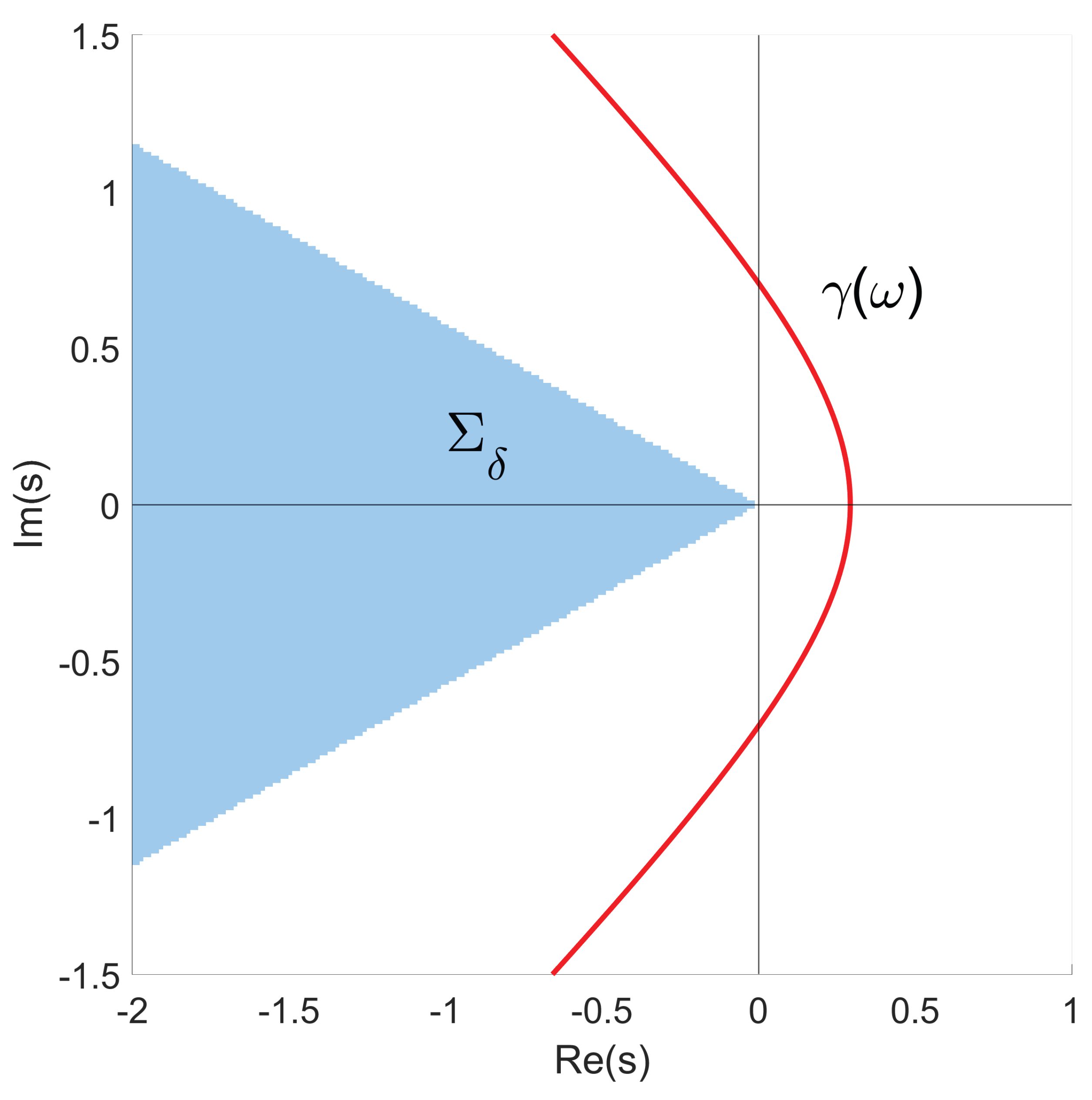
Figure 2.
Influence of on the integration contour
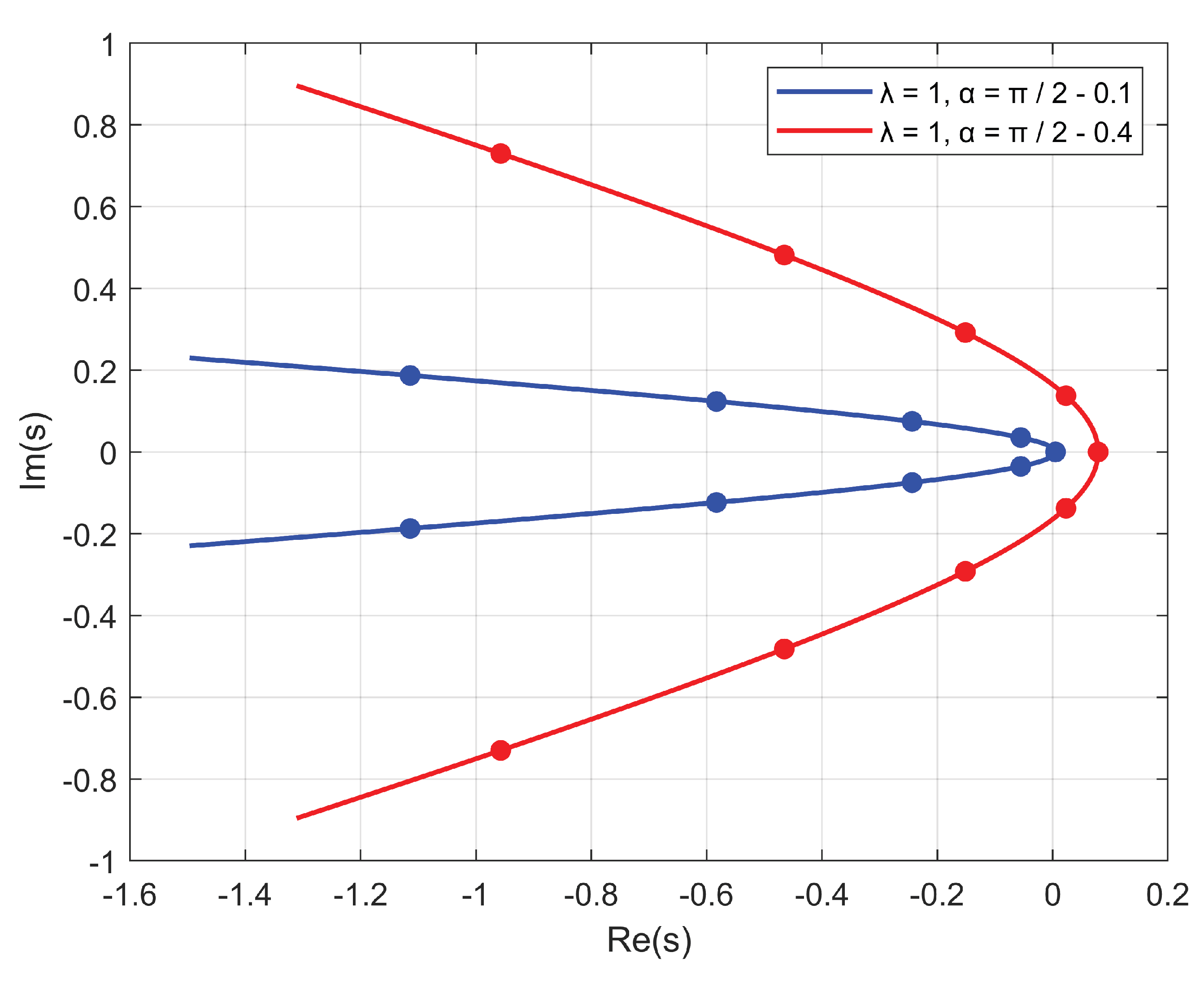
Figure 3.
Influence of on the integration contour
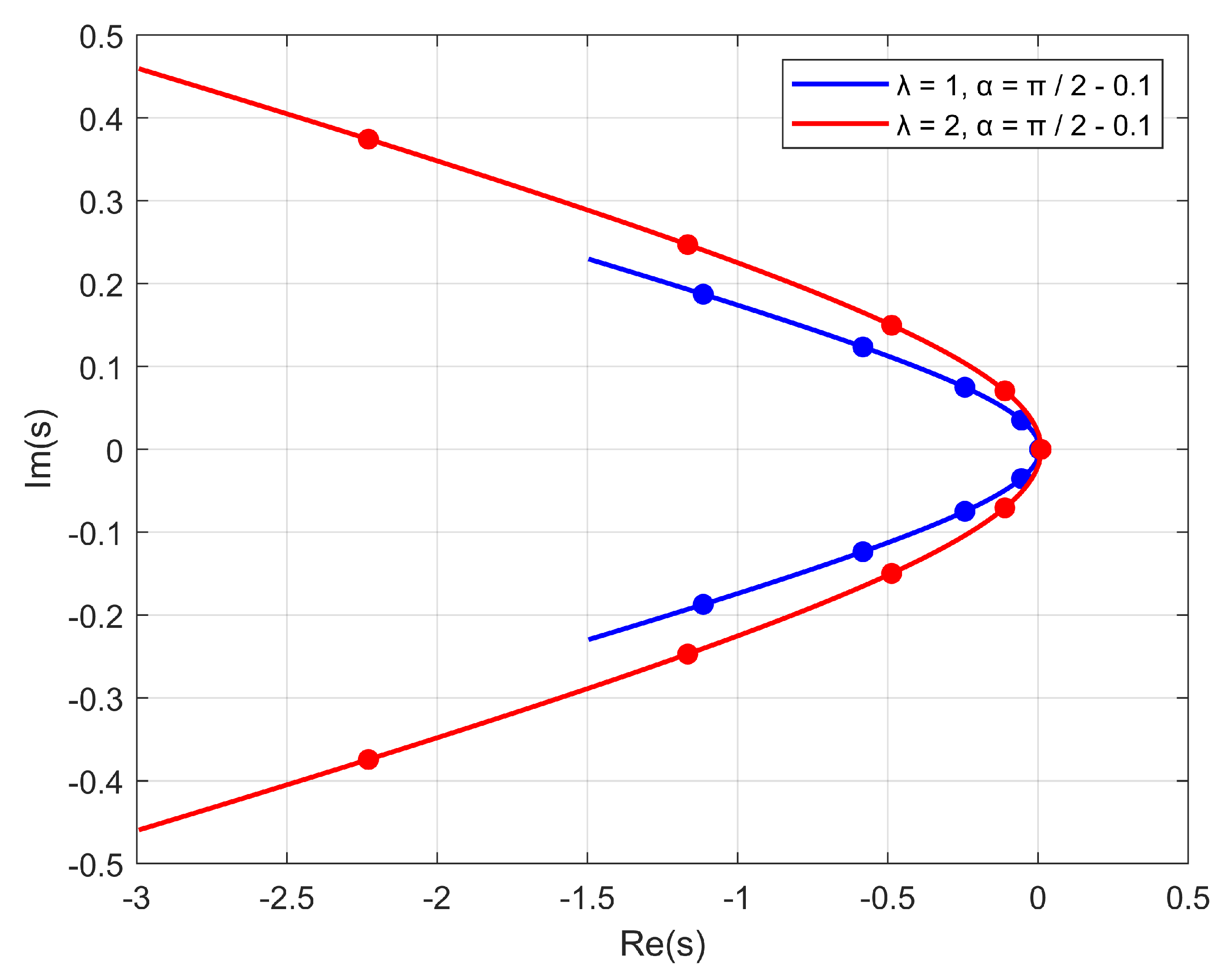
Figure 4.
Boundary surfaces.
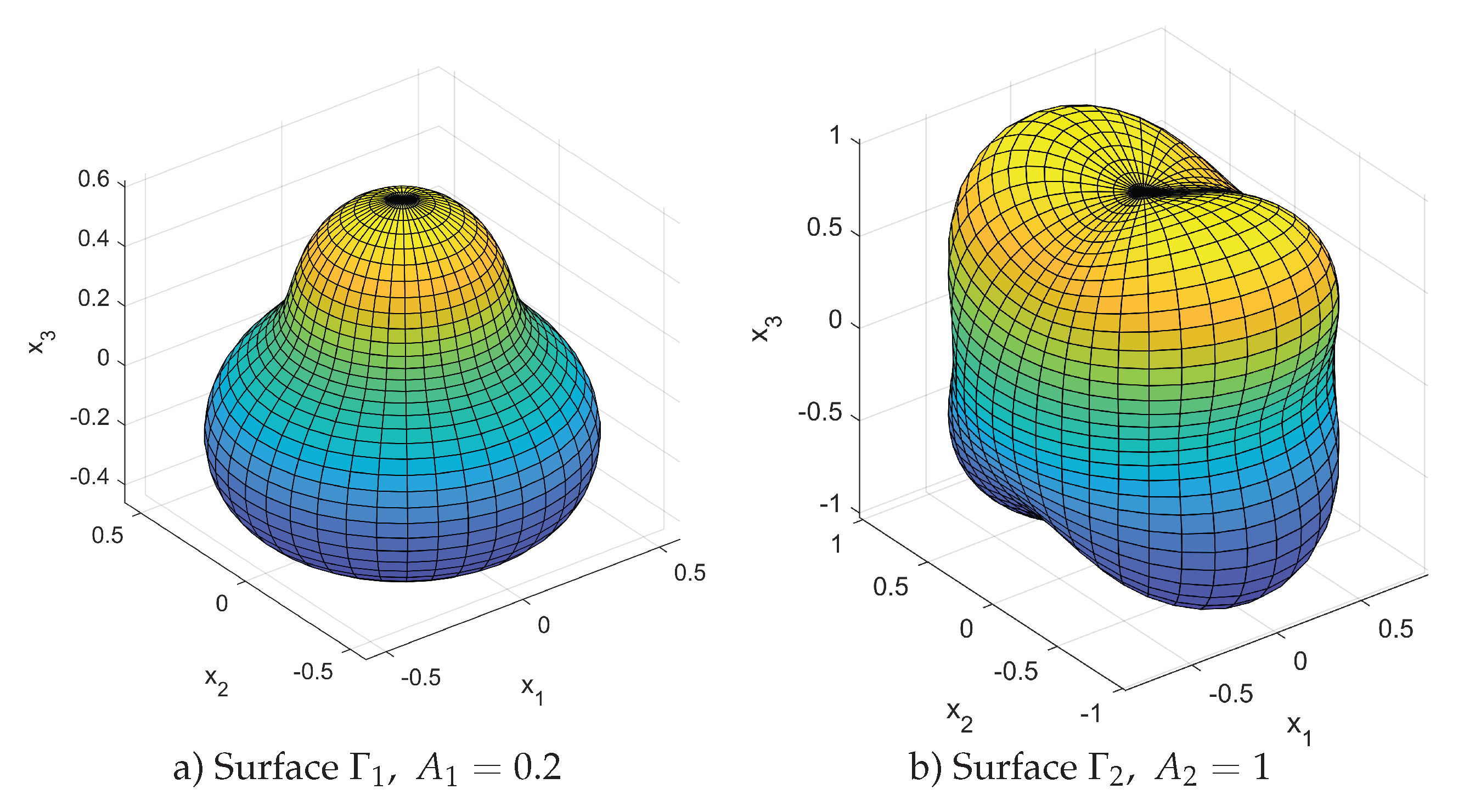
Figure 5.
Numerical solution and boundary condition.
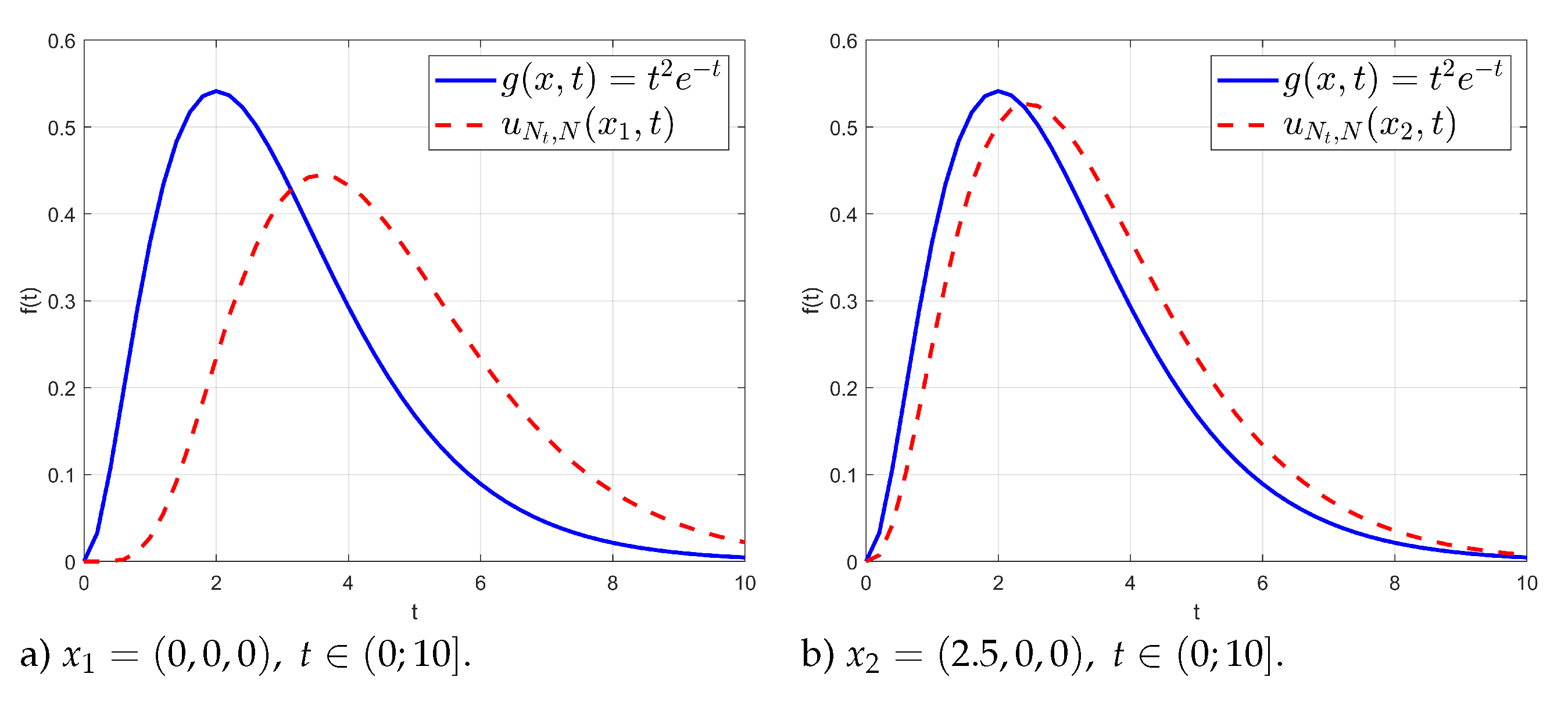
Table 1.
Errors and for
| 2 | 1.27e-08 | 0.989450 | 9.794872 | 2.88e-04 | - 0.2 | 1 |
| 4 | 2.71e-11 | 0.826209 | 5.712821 | 2.00e-05 | - 0.2 | 1 |
| 8 | 1.01e-15 | 1.071071 | 3.671795 | 5.56e-07 | - 0.2 | 1 |
| 16 | 5.45e-20 | 1.071071 | 5.712821 | 8.75e-11 | - 0.2 | 1 |
Table 2.
Errors and for
| 2 | 6.44e-08 | 1.212716 | 8.869492 | 2.98e-04 | - 0.2 | 1 |
| 4 | 1.16e-08 | 1.096689 | 4.822034 | 1.82e-04 | - 0.2 | 1 |
| 8 | 3.11e-15 | 1.058013 | 6.171186 | 3.83e-06 | - 0.2 | 1 |
| 16 | 1.04e-19 | 1.077351 | 9.206780 | 5.59e-09 | - 0.2 | 1 |
Table 7.
Approximate solution for different .
| N | ||||
|---|---|---|---|---|
| 1 | 2 | 4 | 0.35246148 | 0.35659063 |
| 4 | 8 | 0.35245882 | 0.35987086 | |
| 4 | 16 | 0.35246211 | 0.35987241 | |
| 4 | 32 | 0.35246211 | 0.35987241 | |
| 3 | 2 | 4 | 0.45384016 | 0.44480551 |
| 4 | 8 | 0.45327121 | 0.45057778 | |
| 4 | 16 | 0.45327211 | 0.45057821 | |
| 4 | 32 | 0.45327211 | 0.45057821 | |
| 5 | 2 | 4 | 0.17317714 | 0.16828926 |
| 4 | 8 | 0.17226425 | 0.17033565 | |
| 4 | 16 | 0.17225089 | 0.17032869 | |
| 4 | 32 | 0.17225089 | 0.17032869 |
Disclaimer/Publisher’s Note: The statements, opinions and data contained in all publications are solely those of the individual author(s) and contributor(s) and not of MDPI and/or the editor(s). MDPI and/or the editor(s) disclaim responsibility for any injury to people or property resulting from any ideas, methods, instructions or products referred to in the content. |
© 2025 by the authors. Licensee MDPI, Basel, Switzerland. This article is an open access article distributed under the terms and conditions of the Creative Commons Attribution (CC BY) license (http://creativecommons.org/licenses/by/4.0/).
Copyright: This open access article is published under a Creative Commons CC BY 4.0 license, which permit the free download, distribution, and reuse, provided that the author and preprint are cited in any reuse.